Methods in quantum mechanical inverse scattering theory at fixed ...

Methods in quantum mechanicalinverse scattering theoryat fixed energyTamás PálmaiDoctor of Philosophy thesisDepartment of Theoretical PhysicsSupervisor: Barnabás ApagyiBudapest Universityof Technology and EconomicsBudapest, HungaryMay, 2012Copyright c○Tamás Pálmai, 2012

ContentsAcknowledgmentsiChapter 1. Introduction 11. Elements of scattering theory 22. Inverse scattering at fixed energy 5Chapter 2. Newton-type methods 91. Introduction 92. The Newton-Sabatier and Cox-Thompson methods 133. Parity dependent simplification and approximations 184. Consistency investigations 245. Generalization to long-range potentials 28Chapter 3. Transformational procedures 361. Introduction 362. Liouville transformation 363. Using the Gel’fand-Levitan inversion – Horváth-Apagyi method 384. Using the Marchenko inversion 54Chapter 4. Applications to measurement data 611. Introduction 612. Electron-argon potentials 613. Nucleon-alpha potentials 624. Pion-pion quasipotentials 645. Tables and figures 66AppendicesAppendix A. Spectral theory of the one dimensional Schrödinger operator 751. Introduction 752. Definitions 763. Inverse problems 80Appendix B. Special functions 821. Introduction 822. Coulomb wave functions 833. Bessel functions 84Bibliography 90ii

CHAPTER 1IntroductionThe idea of inverse scattering in quantum mechanics was first considered by Heisenberginthe1940s,statingthattheinteractions inaquantumsystemshouldbecompletelydetermined by the scattering matrix. Since then the inverse scattering theory in quantummechanics has been developed and it stimulated much advancement in theoreticalphysics. The inverse problem of potential scattering of a single non-relativistic particlein one dimension was solved by Gel’fand, Levitan, Marchenko and Krein in the 50s[23, 47, 33]. This theory has later led to the discovery of solitonic solutions of certainnonlinear differential equations (e.g. the Korteweg de Vries and non-linear Schrödingerequations) [22, 1]. The quantum version of the so called inverse scattering transformhas been developed later, in the 70s and 80s [32], which have proved instrumental in thedescription of low dimensional quantum systems. On the other hand, the problem onthe scale of potential scattering – the topic of this work – still has undeveloped aspectsand attracts interest, mostly from the nuclear physics community.This thesis is devoted to the development and application of quantum mechanicalinverse scattering methods, which can be used to extract effective central potentialsgoverning the scattering of composite quantum systems. (Potentials obtained by inversescattering methods will be called inverse potentials in this work.) Such methods consistof thedetermination ofamodel independent(effective) central potential inaSchrödingerequation responsible for a scattering picture or cross section data described in terms ofphase shifts. Although one always has some ideas on the range and strength of theinteractions between quantum systems, their exact depth, range and shape are generallyunknown in the more involved or less understood theories (such as the theory behindthe interaction of nuclei). This fact provides the main motivation to develop inversescattering methods.From the methodological point of view this work is concerned with an inverse problem,that of recovering the potential in the Schrödinger equation from scattering data.(Inverse) spectral theoretical methods of the Schrödinger equation are applied and developedto solve this problem. Rigorous treatment of physical, engineering, medical andeven astronomical inverse problems has become a very attractive topic in the field ofapplied mathematics in the last few years. For instance, the famous question: ”Can onehear the shape of a drum?” also boils down to an inverse problem, an acoustic inverseeigenvalue problem [31]. A common property of the interesting inverse problems is thatthey are ill-conditioned (i.e. the solution either does not exists, not unique or not stable[26]) which makes them difficult to solve, usually calling for some stabilization method.The structure of this work is as follows. This chapter introduces further the inversescattering problem of the Schrödinger equation. We start with a short exposition of1

1. ELEMENTS OF SCATTERING THEORY 2scattering theory, then the main facts are gathered on the problem consisting of therecovery of a central potential from the fixed energy scattering phase shifts (equivalently,the cross section data given at one scattering energy). In the main part (chapters2, 3) development of new methods is discussed, which is followed by a short part ofapplications toobtain effective potentials governing quantumsystems frommeasurementdata (chapter 4). It should illustrate the usefulness of the techniques developed inchapters 2 and 3. The underlying mathematical theory (inverse spectral theory of theSturm-Liouville equation) is sketched in Appendix A while some necessary results (someof which are new) on special functions are collected in Appendix B.New scientific results are contained in sections 2.3 [63, 62, 58], 2.4 [56, 58], 2.5[61], 3.2 [59], 3.3 [59], 3.4 [60], 4.2 [61], 4.3, and B.3 [57, 55].1. Elements of scattering theoryWhen describing quantum mechanical scattering it is natural to adopt an operatorialapproach, whichweshall doinitially. Consideraquantummechanical system ofparticlesand let the energy operator be denoted byH = H 0 +Vwith H 0 being the energy operator of the free particles and V the interaction operatorwhich describes a scattering process. Long before (and long after) the collision theinteraction is zero and we have non-interacting particles. Free particles have the timedependentstate vector, Ψ ± (t) which is given byΨ ± (t) = e −iH 0t Ψ ± ,where Ψ ± determines the initial conditions. For finite time the state Ψ(t) is time-evolvedby the whole energy operator, that isΨ(t) = e −iHt Ψ,which satisfieslim ||Ψ(t)−Ψ ±(t)|| = 0.t→±∞The latter can be rewritten aslimt→±∞ ||Ψ−eiHt e −iH0t Ψ ± || = 0.We define the unitary wave operators Ω ± (also known as Møller operators), such thatΩ ± Ψ = limt→±∞ eiHt e −iH 0t Ψ.Another unitary operator, the scattering operator can be defined byS = Ω −1+ Ω −,that relates the asymptotic states: Ψ + ∼ Ω −1+ Ψ ∼ Ω−1 + Ω −Ψ − = SΨ − .There are a number of rigorous results concerning these operators implying theirwell-defined and relevant nature in connection with scattering theory. One of the mostmeaningful results is that for short-range potentials (e.g. in potential scattering shortrangepotentials are those decaying as |x| −1−ε with ε > 0) the wave operators are

1. ELEMENTS OF SCATTERING THEORY 4where δ(k) is the phase shift. Ψ(r) as r → ∞ (r being the distance of the particlefrom the origin or the distance between the two particles) can be viewed as the sum ofincoming and outgoing waves,Ψ(r) = C(k) (e ikr−iδ(k) −e −ikr+iδ(k) )+o(1), r → ∞.2iThe amplitudes of the incoming and outgoing waves are related by the S-matrix whichis expressed asS(k) = e 2iδ(k) .We now move on to the three dimensional case. The time-independent energy eigenstatesof the energy operator will be of central importance for us. For the wave functionΨ(x) = 〈x|Ψ〉 the governing equation reads as(−∇2x +q(x)−k 2) Ψ(k,x,α) = 0, x ∈ R 3 , k ∈ R + , α ∈ S 2where Ψ(k,x,α) is the scattering solution corresponding to the incident direction α andwavenumberk, andisdefinedbyitsasymptotics: Ψ(k,x,α) = e ikx·α +O(1/|x|), |x| → ∞.We supposed the scattering potential to be local, i.e. 〈x|V|x ′ 〉 = V(x)δ(x − x ′ ). It iseasy to see that the next term in its asymptotic expansion is given by(1.1) Ψ(k,x,α) = e ikx·α +A(α ′ ,α,k) eikrkr +o ( 1r), r = |x| → ∞, α ′ = x r .The plane wave e ikx·α is the incident wave and the spherical wave, A(α ′ ,α,k) eikrkris theasymptotic form of the scattered wave. The scattering amplitude A(α,α ′ ,k) is almostthe same as the on-shell T-matrix:A(α,α ′ ,k) = −2π 2 kT( ⃗ k, ⃗ k ′ ), | ⃗ k| = | ⃗ k ′ |.Besides considering local interactions, our second assumption is spherical symmetry,that is q(x) = q(r). Then the expansion of the wave function in terms of sphericalharmonics (Y lm (α)) simplifies to the partial wave expansion,(1.2)(1.3)Ψ(x,α) ==∞∑l∑l=0 m=−l∞∑l=04πi lψ l(k,r)Y lm (α ′ )Ȳlm(α)kr(2l+1)i lψ l(k,r)krP l (cosϑ),where ψ l (k,r) is the lth partial wave – the regular solution (ψ l (k,0) = 0) of the radialSchrödinger equation on the half-line(1.4)(− d2dr 2 + l(l+1) )r 2 +q(r)−k 2 ψ l (k,r) = 0 r ∈ R +and P l (cosϑ) is the lth Legendre polinomial taken at cosϑ = α ·α ′ . It is easy to showthat the regular solution of the radial Schrödinger equation satisfies(1.5)ψ l (k,r) = |F l (k)|r l+1 +o(r l+1 ), r → 0,(1.6)ψ l (k,r) = |F l (k)|sin(kr − lπ 2 +δ l(k))+o(1), r → ∞,

2. INVERSE SCATTERING AT FIXED ENERGY 5|F l (k)| being a constant (i.e. the absolute value of the Jost function, see Appendix A),provided that the potential q(r) decays sufficiently fast as r goes to infinity. The phaseshifts of the partial waves, δ l (k) are defined by the latter asymptotic expression. In thechannel characterized by l the S-matrix takes the form S l (k) = e 2iδl(k) .Similarly to the partial wave expansion for the wave function, the scattering amplitudetakes on a similar form,∞∑ l∑(1.7) A(α ′ ,α,k) = A(α ′ ·α,k) = 4πe iδ lsinδ l Y lm (α ′ )Ȳlm(α)(1.8)l=0 m=−l= 1 2i∞∑(2l +1)(e 2iδ l−1)P l (cosϑ).l=0One can see that the knowledge of the phase shifts is equivalent to that of the scatteringamplitude.We shall be interested in the relationship between the energy operator and the scatteringoperator. The determination of S (or some equivalent quantity) from H is calledthe direct problem while its converse represents the inverse scattering problem in quantummechanics. It is worthwhile to keep in mind that the experimentally availablequantity for measurement is the differential cross section: the ratio of the flux densitiesof the outgoing and incoming particles for a given outgoing direction α ′ . The crosssection (or differential cross section), dσdΩ (α′ ,α,k) is related to the scattering amplitudebydσ(1.9)dΩ (α′ ,α,k) = 1 k 2|A(α′ ,α,k)| 2 .We shall discuss the inverse problem of scattering and for that we need the scatteringamplitude or the phase shifts as input. The scattering amplitude can be recoveredthrough an integral equation for its phase and its modulus (see e.g. [12]). On the otherhand, the phaseshifts can berecovered from the cross section by the so called phase shiftanalysis, which can be carried out as the minimization of the error square expression( ) 2(1.10) χ 2 = 1 dσthN∑ dΩ (ϑ j,k)− dσexpdΩ (ϑ j,k)N ∆ 2 ,(ϑ j ,k)j=1where N is the number of ϑ points where the measurement data, dσexpdΩ (ϑ j,k) is given,dσ thdΩ (ϑ j,k) is the cross section calculated from the theoretical formula with phase shifts{δ l }, which need to be found. ∆ 2 (ϑ j ,k) is the measurement error square of dσexpdΩ (ϑ j,k).It is generally a good strategy to find the global minimum of χ 2 , which however is anontrivial task due to the extreme non-smoothness of χ 2 .2. Inverse scattering at fixed energyThe inverse scattering problem with spherical symmetry is an overdetermined one(to see this, it is enough to consider that the cross section depends on two continuousvariables while the potential to be recovered is a function of only one). Accordingly,there are various cases of special input data of interest. One may formulate methods

2. INVERSE SCATTERING AT FIXED ENERGY 6having the scattering amplitude or the phase shifts as input. Especially important arethe cases when we have fixed angular momentum or fixed energy phase shift. In bothcases we have uniqueness theorems implying the sufficiency of fixed angular momentumor fixed energy data. Note however that the case of mixed data was also investigated[36].Fixed momentum problem is mostly covered by Appendix A, where the inverse scatteringand spectral problems of the one dimensional Schrödinger equation on the halfline is discussed. The only missing ingredient there, is the generalization of the formulation(Jost solutions, spectral function, Gel’fand-Levitan and Marchenko procedures) tosingular potentials which can be found e.g. in [38]. This is because the one dimensionalSchrödinger equation with the potential(1.11) ˜q(r) = q(r)+ l(l+1)r 2is the same as the differential equation of the fixed momentum problem (as l is fixed).The fixed energy problem is much less developed. As early as the 60s it was knownthat the fixed energy phase shifts determine the short-range potential q(r) satisfying(1.12) q(r) = 0, r > a,∫ auniquely [44]. Later this result was sharpened [66, 27]:0r|q(r)|dr < ∞Uniqueness theorem. An infinite subset L, satisfying the Müntz condition,∑ 1l = ∞,l∈L\{0}of the phase shifts is enough to uniquely recover the potential (if complex angular momentaare allowed this condition modifies to the Müntz-Szász condition, ∑ Rl|l| 2 = ∞).Recently it turned out that this requirement is almost necessary [27] in the sensethat a potential with∫ a0r 1−σ |q(r)|dr < ∞, 0 < σ < 2is not determined uniquely by the data with ∑ Rl< ∞.|l| 2On the stability of the inverse scattering problem very little is known. Globally wecan say the following: if the scattering amplitude is bounded by some δ the Fouriertransform of the perturbation of a compactly supported, square integrable and boundedpotential is bounded by log|logδ|/|logδ| [65]. Locally we have [29]||r 2 δq(r)|| L 2 (0,a) ≤ c(1√N+√log 1 εwhere ( ) 2n 2n+2|sinδ(δ n )| < ε, n ≤ Naeand rq(r) is supposedto be boundedand r 2 q(r) having a boundedtotal variation (examplesof such functions include potentials having bounded, continuous derivatives except)

2. INVERSE SCATTERING AT FIXED ENERGY 7at finite points, where jumps are allowed). N is the number of given input phase shifts.The problem with this result is that it gives a bound in terms of an absolute error estimateapplying to all the phase shifts. The desirable scenario would be for relative error.However, the poor convergence of q(x) to the original potential both in the number N ofphase shifts utilized and the absolute error bound (ε) cannot be dismissed. This resultpoints out that potential recovery is unstable, in general. In the course of this thesis itwill become transparent that one might have several, almost phase equivalent potentials(i.e. those generating virtually the same set of phase shifts) as the output of inverse scatteringmethods, when as input only a finite set of phase shifts (even perhaps with error)are known. The choice from these virtually equivalent potentials is often motivated bysome sensible requirement or physical intuition (e.g. by prescribing ∫ ∞0|q(r) ′ |dr to beminimal or |q(0)| < ∞).2.1. A review of inversion methods at fixed energy. From a certain point ofview, the fixed energy problem can be treated on the same footing as the fixed angularmomentum one. Inthelate fifties and inthe sixties aconstructive method was developedby Levitan, Regge, Loeffel and Sabatier [38], similar to the Gel’fand-Levitan theory (seeAppendixA), buildingupontheexistence and uniquenessof thetransformation operator(between free and perturbed solutions) and the spectral decomposition corresponding tothe self-adjoint operator (completeness in l space). The key property is that the inputkernel is a functional of δ l (k), l ∈ R ∪ iR. Thus the data neccessary in this approachis obviously much more than it is physically accessible. To take into account only thephysical phase shifts is not trivial. Indeed, there is no generally accepted method ofinversion at fixed energy. There exist alternatives, however none achieved the eleganceand rigor of their counterparts’ in the fixed angular momentum problem. In essence,there exist two kinds of inverse methods: those relying on inverse spectral theory (e.g.Levitan’s, the Newton-type and the transformational methods) and those using mostlydirect scattering theory. The former ones are sometimes termed as formal methods. Thelatter ones are outside of the scope of this work. Examples of these methods include theiterative-perturbative [46] and WKB methods of which reasonable amount of experiencehas been collected, for a survey see [34]. Another such interesting procedure consists ofapproximating the S-matrix in term of a rational fraction which gives rise the so calledBargmann potentials, whose forms are known explicitly from the S-matrix [40, 41]. Thecommon element of these procedures is the introduction of some kind of a theoreticalapproximation.One of the most popular family of inversion techniques at fixed energy consists ofthe Newton-type, or matrix methods [12]. They strongly depend on the existence anduniqueness [66] of an l-independent transformation kernel. Then a Gel’fand-Levitan-Marchenko type integral equation (cf. (A.41)) is supposed for this kernel. For the inputkernel in the a Gel’fand-Levitan-Marchenko-type (GLM) integral equation an angularmomentum decomposition is postulated, which only depends on the potential througha finite number of coefficients. A relation between the coefficients and the phase shiftsis derived (either linear or non-linear) and through its application the potential can beobtained. These type of methods are easy to use, however only capable to look forpotentials in a very specific class. In addition there are theoretical concerns: uniquesolvability of the GLM type equation must be maintained, otherwise the method breaks

2. INVERSE SCATTERING AT FIXED ENERGY 8down [68], which aspect of these methods still requires development. The matrix methodsare discussed in Chapter 2.Recently, we developed another family of exact methods. It utilizes a Liouvilletransformation of the fixed energy radial Schrödinger equation to obtain its Liouvillenormal form (cf. AppendixAand seeChapter 3). Then, it turnsout that the m-functionof the resulting operator is given in discrete points by the fixed energy phase shifts. Them-function is meromorphic and determines the potential, which two properties suggestthe possibility of a scheme to recover the potential from the m-function values. Thesenew methods are discussed in Chapter 3.

CHAPTER 2Newton-type methods1. Introduction1.1. General framework at fixed energy. The fixed energy problem is formulatedin terms of the radial Schrödinger equation for the partial waves,)(2.1)(− d2 l(l +1)+dr2 r 2 +q(r) ψ l (r) = k 2 ψ l (r) l = 0,1,2,...,with a potential satisfying(2.2)(2.3)∫ 10r|logrq(r)|dr < ∞,∫ ∞1r|q(r)|dr < ∞.These conditions specify a standard scattering class (made up of functions decayingmore rapidly than r −1 and not too singular in the origin) and a short-ranged scatteringpotential can assumed to be in this class.We fix k = 1 which does not lead to the loss of generality. Indeed, the dimensionfulreduced potential is recovered as q DIM (r) = k 2 q(kr). Then (2.1) can be turned into theeigenvalue equation(2.4) D(r)y(r) = λ 2 y(r),given in λ = l+ 1 2 , l = 0,1,2,... and y(r) = 2ψ r−1 l (r). The operator D(r) is(2.5) D(r) = D 0 (r)−r 2 q(r) = r d (r d )+r 2 −r 2 q(r), 0 < r < ∞,dr drwhere D 0 (r) with a vanishing potential is also implicitly defined. Also, let ∆ 0 (r) =D 0 (r)−r 2 , which only contains the first term from the RHS of (2.5).Now, following [38] I introduce the spectral formalism for the fixed energy problem.It turns out, that the Gel’fand-Levitan theory (see Appendix A) can be transferred tothe fixed energy problem with little modification. The Gel’fand-Levitan theory reliesupon the spectral decomposition of the operators D and D 0 (or equivalently that of ∆ 0 )and transformation operators which transform the solutions of the eigenvalue equationsdefined by the previous differential operators into each other. In this framework spectraldata (which can in ideal cases be connected to scattering data) determines an inputkernel, which gives the potential via the solution of an integral equation. In our case,however, the scattering data is insufficient to obtain the input kernel. Nevertheless, theformalism is still useful as it turns out.9

1. INTRODUCTION 10First the boundary condition is specified. Let us denote the solutions to the eigenvalueequations behaving regularly at the origin by φ ∆0 ,D 0 ,D(r,λ), i.e.,(2.6) φ ∆0 ,D 0 ,D(r,λ) →r λ2 λ Γ(λ+1) , r → 0.It can be shown that only one of the two linearly independent solutions to the eigenvalueequations behaves regularly (thus the operators are limit point at the origin). We willconsider regular solutions. The spectral decompositions are given by(2.7)12∫ ∞−∞φ ∆0 (r,iτ)φ ∆0 (r ′ τdτ,−iτ)sinhπτ = rδ(r −r′ )(2.8)∞∑2λ n φ D0 (r,λ n )φ D0 (r ′ ,λ n )n=1+ 1 2∫ ∞−∞(φ D0 (r,iτ)− µ )0(−iτ)µ 0 (iτ) φ D 0(r,−iτ)φ D0 (r ′ τdτ,−iτ)sinhπτ = rδ(r −r′ )(2.9)∞∑ 1||φ D (r,λ n )|| 2φ D(r,λ n )φ D (r ′ ,λ n )+ 1 ∫ ∞(φ D (r,iτ)− µ(−iτ) )2 µ(iτ) φ D(r,−iτ) φ D (r ′ τdτ,−iτ)sinhπτ = rδ(r −r′ )n=1−∞rNotethatφ ∆0 (r,λ) =λ2 λ Γ(λ+1) andφ D 0(r,λ) = J λ (r), thelatterbeingtheBesselfunctionof the first kind. For the other quantities λ n , µ 0 , µ and ||...|| 2 see [38].The transformation operators are defined as in Appendix A, but now the integrationmeasure is 1 r, thus a transformation operator X applied to a function f(r) gives(2.10) Xf(r) = f(r)+∫ r0A(r,t)f(t) dtt ,with some kernel A(r,t). The kernels A ∆0 ,D, A D0 ,D belonging to the transformationoperators X ∆0 ,D : φ ∆0 → φ D , X D0 ,D : φ D0 → φ D , respectively, satisfy appropriatedifferential equations with boundary conditions(2.11) A ∆0 ,D(r,r) = − r24 + 1 2∫ r0sq(s)ds(2.12) A D0 ,D(r,r) = 1 2∫ r0sq(s)dsThe Gel’fand-Levitan-type integral equations are in the form(2.13) 0 = A B,D (r,r ′ )+F B,D (r,r ′ )+∫ r0A B,D (r,r ′′ )F B,D (r ′′ ,r ′ ) dr′′r ′′ ,r′ < r

1. INTRODUCTION 11where B is one of ∆ 0 and D 0 . Similarly to (A.43) the kernels are of the form(2.14)(2.15)F ∆0 ,D(r,r ′ ) =F D0 ,D(r,r ′ ) =which can be expressed explicitly as∫ ∞−∞∫ ∞−∞φ ∆0 (r,λ)φ ∆0 (r ′ ,λ)dσ ∆0 ,D(λ)φ D0 (r,λ)φ D0 (r ′ ,λ)dσ D0 ,D(λ)(2.16) F ∆0 ,D(r,r ′ ) = f(rr ′ )with(2.17) f(r) =and∞∑n=1(2.18) F D0 ,D(r,r ′ ) =1a 2 − 1 ∫ ∞n4 λn Γ(1+λ n ) 2rλn 2 −∞n=0µ(−iτ) τdτ4 iτ Γ(1−iτ) 2 µ(iτ) sinhπτr iτ∞∑∞∑J λn (r)J λn (r ′ )− 2nJ 2n (r)J 2n (r ′ )n=1∫ ∞− 1 2−∞( µ(−iτ)µ(iτ) +1 )J iτ (r)J iτ (r ′ τdτ)sinhπτThe quantities λ n and µ appearing in the input kernels are functionals of the phase shiftfunction δ(λ) defined by the asymptotic behaviour of the solution φ D (r,λ),( πr) −1(2(2.19) φ D (r,λ) = A(λ)sin r − π (λ− 1 ) )+δ(λ) +o(1), r → ∞,2 2 2and δ(λ) is required for real and pure imaginary λ’s. Note that the uniqueness theoremof Chapter 1 suggests that δ(λ) could be obtained for the nonphysical arguments fromthe physical data, however there is no such procedure currently available.Now, suppose that the potential q(r) is the restriction of an entire function to thehalf line. In this case it can be shown that the input kernels admit the expansions∞∑ ∞∑(2.20) F ∆0 ,D(r,r ′ ) = a n (rr ′ ) n + a n+1/2 (rr ′ ) n+1/2(2.21) F D0 ,D(r,r ′ ) =(2.22)(2.23)(2.24)n=1n=1n=0∞∑∞∑c n J n (r)J n (r ′ )+ c n+1/2 J n+1/2 (r)J n+1/2 (r ′ )For further reference let us give (2.13), (2.10), (2.21) for the functionsNamely, we have(2.25) K(r,r ′ ) = g(r,r ′ )−n=0K(r,r ′ ) = − √ rr ′ A ∆0 ,D(r,r ′ ),g(r,r ′ ) = √ rr ′ F ∆0 ,D(r,r ′ ),ψ l (r) = √ rφ D (r,λ−1/2).∫ r0K(r,t)g(t,r ′ ) dtt 2, r ≥ r′ ,

1. INTRODUCTION 12with(2.26)where(2.27)(2.28)Further,(2.29) ψ l (r) = u l (r)−L r K(r,r ′ ) = L y0 K(r,r ′ ), 0 < r ′ ≤ r,q(r) = − 2 rddrK(r,r), K(r,0) = 0r]L r =[r 2 d2dr 2 +r2 −r 2 q(r)]L r0 =[r 2 d2dr 2 +r2 .∫ r0K(r,r ′ )u l (r ′ )r ′ −2 dr ′ , K(r,0) = 0where u l (r) is the lth Riccati-Bessel function,√ πr(2.30) u l (r) =2 J l+ 1 (r)2which is the regular solution of the free radial Schrödinger equation (q ≡ 0). Theexpansion for the restriction of analytic potentials can be written as∞∑∞∑(2.31) g(r,r ′ ) = c ′ n u n−1/2(r)u n−1/2 (r ′ )+ c ′ n+1/2 u n(r)u n (r ′ ).n=11.2. Matrix methods. While the above general formulation is very appealing, itis not apparent how it is useful when solving the inverse problem at fixed energy, i.e.determining the potential from the fixed energy physical phase shifts. The problem isthat thephaseshiftsrequiredfortheconstruction oftheinputkernelaremuchmorethanaccessible physically (i.e. phase shifts not only for non-integer but also for imaginaryangular momenta).Newton-type methods solve this problem by taking the expansion (more preciselyonly a part of) (2.31) and determining the coefficients from the phase shifts throughtaking the r → ∞ limit of the Povzner-Levitan representation (2.29). We note, thatindependent of the above construction the existence of K(r,r ′ ) in (2.29) satisfying theGoursat-type problem (2.26) was shown in [66].The differential equation for the transformation kernel implies in turn for g(r,r ′ )(2.32) L r0 g(r,r ′ ) = L r ′ 0g(r,r ′ ), g(r,0) = g(0,r ′ ) = 0.If only looking at this equation one can see that g(r,r ′ ) is a good candidate for approximationsince its differential equation can be satisfied trivially, for instance if the angularmomentum expansionn=0(2.33) g(r,r ′ ) = ∑ lc l γ l (r,r ′ ),

2. THE NEWTON-SABATIER AND COX-THOMPSON METHODS 13is imposed then for the γ l (r,r ′ ) functions we only have the potential-independent restrictionsof(2.34) L r0 γ l (r,r ′ ) = L r ′ 0γ l (r,r ′ ), γ l (r,0) = γ l (0,r ′ ) = 0, ∀l.and the information is put in the c l expansion coefficients.However thisisnotcompletely true. Notethatbyapproximatingtheinputkernelonemight introduce inconsistency to one’s method. This is because the angular momentumdecomposition with arbitrary coefficients does not yield, in general [68], a potential evenif the differential equation for the input kernel g(r,r ′ ) is satisfied. The reason for this liesin the fact that the fulfillment of the differential equation is not sufficient for the GLMtypeintegral equation to be uniquely solvable. This problem was the source of confusionin the literature and this line of thought is continued in section 4 (in the context of theCox-Thompson method), for now it is supposed that equation (2.25) is uniquely solvablewith g(r,r ′ ).Another feature is that depending on the basis functions quite different procedurescan be obtained. In the Newton-Sabatier procedure we take γ l (r,r ′ ) = u l (r)u l (r ′ ) whichyields a linear problem in terms of the data for the coefficients. This method in itselfcontains a parameter that must be chosen to get a potential which decays faster thanthe others at infinity. The Newton-Sabatier method was later modified by Münchowand Scheid truncating the range of the inversion, taking q(r) = 0, r > a [52]. Thistruncation proved to be highly beneficial and the subsequent mNS method was usedby various authors in the 80s and 90s to obtain effective potentials governing quantumsystems, mainly of nuclear physical interest. The mNS method while linear thus easy tohandle has some drawbacks most prominently producing potentials being singular at theorigin, contrary to the frequent assumption of non-singular behavior for nuclear physicalpotentials at the origin. To overcome this difficulty it turns out that one must take adifferent ansatz for the γ l (r,r ′ ) functions. Taking the Cox-Thompson prescription [14]producespotentials generally beingfiniteat theorigin however it also entails abandoningthe linear problem for a nonlinear one.2. The Newton-Sabatier and Cox-Thompson methods2.1. Newton-Sabatier method and its modification. Starting from the ansatzimposed on the symmetric kernel∞∑(2.35) g(r,r ′ ) = c l u l (r)u l (r ′ ),l=0one obtains the Newton-Sabatier method. This prescription is ”half” of the series (2.31),thus ideal convergence properties are not expected for a general potential. On the otherhand the method yielded is easily applicable and is indeed one of the most frequentlyused inverse scattering procedure.If the Newton-Sabatier expansion is substituted into the integral equation one gets∞∑∫ ∞∞∑(2.36) K(r,r ′ ) = c l u l (r)u l (r ′ )− dr ′′ r ′′ −2 K(r,r ′′ ) c l u l (r ′′ )u l (r ′ ),l=00l=0

2. THE NEWTON-SABATIER AND COX-THOMPSON METHODS 14which in view of the PL representation (2.29) implies(2.37) K(r,r ′ ) =∞∑c l ψ l (r)u l (r ′ ).This is then substituted into the PL representation with the result∞∑(2.38) ψ l (r) = u l (r)− c l ′L ll ′(r)ψ l ′(r),where(2.39) L ll ′(r) =∫ r0l=0l ′ =0{ ∫ rdtt −2 0u l (t)u l ′(t) =dtt−2 u 2 l(t) l = l′W[u l ,u l ′](r)l ′ (l ′ +1)−l(l+1)l ≠ l ′given explicitly in terms of the Wronskian W[a,b] = ab ′ −a ′ b for l ≠ l ′ . This equationis then taken at x → ∞, whereψ l (r) = B l sin(r −lπ/2+δ l )+o(1),x → ∞applies and an infinite system of linear equation is yielded for B l ’s and c l ’s. However,the solution of this system of equations is not unique, which problem, in theory, can beremedied by choosing the solution giving rise to the most decaying potential [71]. Inaddition the potentials have zero first momenta (which is consistent with an undesirableoscillation at large distances) and possess a non-physical simple pole at x = 0. All inall, the Newton-Sabatier method is considered impractical, with good reason.There is a modification [52] of this procedure, however, which is applicable to treatpotentials with compact support, [0,a]. In this case(2.40) ψ l (r) = A l (cos(δ l )u l (r)−sin(δ l )v l (r)) ≡ A l α l (r), r > aapplies for the partial waves, which is definite for any r, in terms of the phase shifts. Ifthis is substituted into (2.38) one getsl∑max(2.41) A l α l (r) = u l (r)− c l ′A l ′L ll ′(r)α l ′(r) l ∈ S ≡ {0,1,...,l max }.l ′ =0Let c l A l = C l and a kl (r) = α l (r)δ kl where δ kl is the Kronecker-delta. Then (2.41) turnsinto∑(2.42) akl (r)A l = u l (r)− ∑ L kl (r) ∑ a ll ′(x)C l ′ k ∈ S.Let nowandM k ={A k , k ≤ l maxC k−lmax , k > l max{a lk (x) k ≤ l maxN lk = ∑ lmaxk ′ =0 L lk ′(r)a k ′ k(r) k > l max ,

2. THE NEWTON-SABATIER AND COX-THOMPSON METHODS 15then one gets the system of linear equations(2.43)2l∑ maxk=0N lk (r)M k = u l (r), l ∈ S.This system is underdetermined for a single r 1 parameter, however, if it is used in morer i points simultaneously it is solvable, per se. Moreover for three of more r i ’s it isoverdetermined and one can use a least squares method to get a solution. In case ofdata with considerable errors, solving the overdetermined system of equations for thecoefficients can be beneficial. Indeed, the result might also vary as the r i points arevaried, which is to be avoided and generally some stability examination is necessary.If the coefficients c l are obtained, the potential is yielded by(2.44)q(r) =− 2 r=− 2 rddrl∑maxl=0( ∑lmax)l=0 c lu l (r)ψ l (r)r[ u′c l · l(r)ψ l (r)+ u l(r)ψl ′(r)− u ]l(r)ψ l (r)r r r 2 ,readily, where ψ l (r) and ψl ′ (r) is to be calculated from (2.38) and its derivative. Anobvious advantage of this procedure is its linearity: only linear systems of equationsneed to be solved. Nevertheless, the non-physical pole at the origin is still a (sometimesunwanted) feature of this mNS method.2.2. Cox-Thompson method. In the framework of the method proposed by Coxand Thompson [14] one takes the following separable form for the γ l (r,r ′ ) functions(2.45) γ l (r,r ′ ) = u l (min(r,r ′ ))v l (max(r,r ′ )),which is also the Green’s function of the q ≡ 0 radial Schrödinger equation for the lthpartial wave:[ ] d2l(l+1)(2.46)+1−dr2 r 2 γ l (r,r ′ ) = δ(r −r ′ );and the summation in g(r,r ′ ) runs only over a finite set S of input physical angularmomenta, l’s:(2.47) g(r,r ′ ) = ∑ l∈Sc l u l (min(r,r ′ ))v l (max(r,r ′ )),containing the Riccati-Bessel functions (regular and irregular solutions of the free radialSchrödinger equation), connected to the Bessel and Neumann functions by√ √ πrπr(2.48) u l (r) =2 J l+ 1 (r), v l (r) =2 2 Y l+ 1 (r).2Taking such an expansion can be interpreted as going beyond the expansion (2.31)coming from the general framework for a potential being the restrictions of analyticfunctions. Also, one can view the Cox-Thompson ansatz as a resummation of (2.31).

2. THE NEWTON-SABATIER AND COX-THOMPSON METHODS 16For solving the GLM-type equation (2.25) we use the separable ansatz(2.49) K(r,r ′ ) = ∑ L∈TA L (r)u L (r ′ )with a finite set T of ”shifted angular momenta” satisfying S∩T = ∅ and |S| = |T|. Theuse of such an ansatz can be motivated by the following result ascertained from [13, 58].Proposition 1. If y −1/2 K(r,r ′ ) = O(1), y → 0 is imposed on K(r,r ′ ) and the Lnumbers are restricted to L > −0.5 then∏L∈T(l(l +1)−L(L+1))(2.50) c l = ∏l ′ ∈S,l ′ ≠l (l(l +1)−l′ (l ′ ⇔ K(r,r ′ ) = ∑ A L (r)u L (r ′ ).+1))L∈TWhere {c l } ↔ {L} is a one-to-one mapping.Also, this form provides a reasonably easy way to solve the GLM-type integral equation.In fact, it makes two (independent) systems of algebraic equations instead of theintegral equation, namely that of (2.50) and(2.51)∑L∈TA L (r) u L(r)v ′ l (r)−u′ L (r)v l(r)l(l+1)−L(L+1)= v l (r), l ∈ S.The parameters of the set T can be obtained from the phase shifts {δ l } l∈S throughthe transformation equation (2.29), which in terms of the L’s takes the form(2.52) ψ l (r) = u l (r)− ∑ L∈TA L (r) u L(r)u ′ l (r)−u′ L (r)u l(r)l(l+1)−L(L+1)Taking both equation (2.52) and (2.51) for large r’s, i.e. r → ∞ we get the system ofnonlinear equations [4, 51, 63] connecting {δ l } l∈S to T:(2.53) e 2iδ l= 1+iK+ l1−iK − lalternatively, l ∈ S,K + l+K − l(2.54) tanδ l =2+i(K + l−K − l ∈ S,l),with(2.55) K ± l= ∑ ∑[M sin ] lL [Mcos] −1 Ll ′e ±i(l−l′ )π/2l ∈ S,L∈T l ′ ∈S{ }{Msin 1 sin((l−L)π/2)(2.56) =M cos L(L+1)−l(l+1) cos((l−L)π/2)lLThe potential is expressed as(2.57)q(x) = 2 K(x,x)x 3 −2 K′ (x,x)x 2 = 2 ∑ [AL (x)u L (x)x 3 − A L(x)u ′ L (x)+A′ L (x)u ]L(x)x 2 ,Lwhere the differentiation can be performed analytically and A L (x), A ′ L(x) are calculatedfrom equation (2.51).}.

2. THE NEWTON-SABATIER AND COX-THOMPSON METHODS 172.2.1. Asymptotics. Concerning the asymptotics of the CT potential, first we showthat the potential is generally not compactly supported nor is of long-range. To see thisdefine the functions {A a L (r)} L∈T by the limit(2.58) A L (r) = A a L (r)+o(1), r → ∞, L ∈ T.Take the asymptotic version of equation (2.51),∑(2.59) A a cos((l −L) π 2L(r))l(l +1)−L(L+1) = −cos(r −lπ ), l ∈ S,2L∈Tand differentiate it twice with respect to the variable r. Thend 2 A a L(2.60)(r)dr 2 = −A a L (r),is obtained, which admits a periodic solution [63](2.61) A a L(r) = a L cos(r)+b L sin(r),where a L ’s and b L ’s are constants depending on all the elements of both S and T:∑ cos( π 2(2.62) a (l−L))L(lL(L+1)−l(l +1) = cos π ), l ∈ S,2(2.63)L∈T∑L∈Tb LThis form in turn implies thatcos( π 2(l −L)) (lL(L+1)−l(l+1) = sin π ), l ∈ S.2(2.64) K(r,r) = αsin(2r)+βcos(2r)+γ +o(1), r → ∞and thus(2.65) q(r) = βsin(2r)−αcos(2r)r 2 ·(1+o(1)), r → ∞.Which means that the potential generally falls of as a second inverse power.One can give a necessary condition for the potential to decrease more rapidly thenO(r −2 ) [58]. One only needs(2.66) α = β = 0.The quantities α and β are given byα = 1 ∑ (a L cosL π 2 2 −b LsinL π )(2.67)2L∈Tβ = − 1 ∑(a L sinL π 2 2 +b LcosL π )(2.68).2L∈TAlternatively, K(r,r) can be written as a series in l (this formula does not hold forK(r,r ′ ) with r ≠ r ′ ),(2.69) K(r,r) = ∑ l∈Sc l ψ l (r)v l (r),

3. PARITY DEPENDENT SIMPLIFICATION AND APPROXIMATIONS 18which can readily be seen from the GLM equation (2.25) taken at r = r ′ and the CTformula (2.45) substituted for g(r,r ′ ):(2.70)(2.71)K(r,r) = ∑ l∈S= ∑ l∈Sc l u l (r)v l (r)−[c l v l (r) u l (r)−∫ r0∫ rdtt −2 K(r,t) ∑ l∈S]K(r,ρ)u l (t)t −2 dt ,0c l u l (t)v l (r)where the formula (2.29) for ψ l (r) has appeared. This allows for the alternative conditions∑∑(2.72) (−1) l c l B l cosδ l = 0, and (−1) l c l B l sinδ l = 0l∈Sinvolving the expansion coefficients, the input phase shifts and the normalization constantsof the partial wave functions.Such results may serve as useful tools to check numerical results or incorporated intoa solution method providing a way to control the undesirable oscillations of the inversepotential.Second, we note that the potential at the origin is given by(2.73) q(r) = Q−2(1−Q)∑L∈T,l∈Sl∈SG −1lL2l −1 +O(r2 ), r → 0coming from the power series of the Bessel functions appearing in the explicit formulasfor q(r), containing the inverse of the G matrix with elements(2.74) [G] Ll = 1L−land Q = ∑L∈T,l∈SG −1lLL+ 3 .2Thisform showsthat thepotential starts at theorigin with zero derivative and, generallyfrom a finite value |q(0)| < ∞.Three aspects of the Cox-Thompson method are discussed in the remainder of thischapter: i) simplifications of the system of nonlinear equations and the introduction ofsome approximative solutions, ii) consistency of the method and iii) generalization toefficiently treat long-ranged potentials with known asymptotics far from the origin.3. Parity dependent simplification and approximationsIn this section we present simplifications to equations (2.53) which can be used ifonly even (odd) partial waves are arising during the collision. Otherwise the simplifiedequations can be employed to construct different approximations which will be discussedin separate subsections [63, 62].3.1. Even (odd) angular momentum treatment. Inserting the periodic solution(2.61) into equation (2.59) and taking into account the independence of the sineand cosine functions, one gets the following two equations∑{ } ( )aL cos (l−L)π { ( ) }2 cos lπ(2.75)b L L(L+1)−l(l+1) = 2sin ( l π ) , l ∈ S.2L∈T

3. PARITY DEPENDENT SIMPLIFICATION AND APPROXIMATIONS 19Consider the decompositionS = S e ∪S owhere S e and S o contains, respectively, the even and odd elements of S. Instead of (2.59)we consider two systems:∑} ( )cos (l −L)π { ( ) }2 cos lπb L L(L+1)−l(l+1) = 2sin ( l π ) , l ∈ S e2andL∈T e{aL∑L∈T o{aL} ( )cos (l −L)π { ( )2 cos lπb L L(L+1)−l(l+1) = 2sin ( l π )2}, l ∈ S o ,where |T e | = |S e |, |T o | = |S o | and T e ∩ S e = ∅, T o ∩ S o = ∅. These systems have thesolutions∏l∈S(2.76) a L = e(L(L+1)−l(l +1)) 1∏L ′ ∈T e\{L} (L(L+1)−L′ (L ′ +1)) cos ( L π ), b L = 0, L ∈ T e ,2and∏l∈S(2.77) a L = 0, b L = o(L(L+1)−l(l+1)) 1∏L ′ ∈T o\{L} (L(L+1)−L′ (L ′ +1)) sin ( L π ), L ∈ T o ,2respectively. In case of T e ∩T o ≠ ∅ the formulae (2.76) and (2.77) may assign differentvalues to the same a L and b L butthis is not a real ambiguity because the solution vectors(2.76) and (2.77) are always used separately.Now, by using the explicit expressions (2.76) in equations (2.61) and the asymptoticversion of (2.29), one obtains a simplified equations instead of (2.53):(2.78) tan(δ l ) = − ∑ ∏l ′ ∈S e\{l} (L(L+1)−l′ (l ′ +1))∏(LL∈T eL ′ ∈T e\{L} (L(L+1)−L′ (L ′ +1)) tan π ), l ∈ S e ,2valid for the case of even l’s. Similarly, using equations (2.77) we get the system ofequations(2.79) tan(δ l ) = ∑ ∏l ′ ∈S o\{l} (L(L+1)−l′ (l ′ +1))∏(LL∈T oL ′ ∈T o\{L} (L(L+1)−L′ (L ′ +1)) cot π ), l ∈ S o2which are valid in the case of odd l’s.Noticethesimplifiedstructureofthenonlinearequations(2.78)and(2.79), comparedto equations (2.53). While equations (2.53) contain an implicit matrix inversion of thematrix M cos involving the unknowns of shifted angular momenta, L’s, formulas (2.78)and (2.79) do not require such a nonlinear operation. They ’only’ contain products andthe tangent (cotangent) operations and are thus presumably easier to be solved for thesets T e or T o , if the respective input phase shifts are given.Findingthesets T e or T o , thecorrespondingpotentials V e (r) or V o (r) can beobtainedsimilarly as in the general case, by employing equations (2.51), (2.49), and (2.26).

3. PARITY DEPENDENT SIMPLIFICATION AND APPROXIMATIONS 203.2. Equivalence of solutions (2.53) and (2.78) or (2.79). By explicit calculationone can check the equivalence of equations (2.53) and (2.78) or (2.79) for the specialcases of even or odd l’s. For the case of either even or odd l’s, the relation K + l= K − lholds. Now, specifying ourselves to the even l case only, l ∈ S e , the general equations(2.53) can be written as(2.80) tan(δ l ) = ∑[M sin ] lL [Mcos −1 ] Ll )/2 ′(−1)(l−l′ , l ∈ S e .L∈T e,l ′ ∈S eUsing (2.59) and (2.61) we get the expression(2.81) a L cos(r) = ∑cos] Ll ′ cos(r −l ′π 2 ),which simplifies to(2.82) a L = ∑l ′ ∈S e[M −1l ′ ∈S e[M −1cos] Ll ′(−1) l′ /2 , L ∈ T e .L ∈ T eBy multiplying both sides of these equations by (−1) l/2 [M sin ] lL , and performing the sumover L’s, one may write∑(2.83) a L [M sin ] lL (−1) l/2 = ∑[M sin ] lL [Mcos] −1 Ll ′(−1) (l−l′)/2 , l ∈ S e .L∈T e L∈T e,l ′ ∈S eAccording to equation (2.80) the right hand side is already equal to tan(δ l ) and bynoting that the matrix M sin on the left hand side can be written, on account of (2.56),as [M sin ] lL = −(−1) l/2 sin(L π 2)/(L(L+1)−l(l+1)) one gets the formula(2.84) tan(δ l ) = − ∑ L∈T ea Lsin(L π 2 )L(L+1)−l(l+1) ,l ∈ S ewhich is the same as equation (2.78) if one takes into consideration the solution (2.76)for the coefficient a L ,L ∈ T e .A similar procedure can be applied to proving equivalence of equations (2.53) and(2.79) for odd l’s.3.3. Asymptotics. For potentials constructed from phase shifts belonging to partialwaves of a single parity the CT inverse potential behaves in a peculiar manner [58].To see this we derive the phase shifts of the CT potential.Phase shifts of the inverse potential can be get from equation (2.52) if it is taken atr → ∞:(2.85) ψ j (r) = sin(r −jπ/2) − ∑ L∈TA a L (r) sin((j −L)π/2)+o(1), r → ∞.j(j +1)−L(L+1)Now the trigonometric form (2.61) is substituted for A a L(r). There are two special casesthat we consider: i) the S set (of input angular momenta) consists of only even numbers,ii) S consists of odd numbers. In the first case we have b L = 0 ∀L ∈ T while in the

3. PARITY DEPENDENT SIMPLIFICATION AND APPROXIMATIONS 21second a L = 0 ∀L ∈ T. This is deductible from equations (2.62) and (2.63) which assumethe forms∑{ }aL cos ( L π ) { }2 1(2.86)b L L(L+1)−l(l+1) = , l ∈ S0L∈T∑{ }aL sin ( L π ) { }2 0(2.87)b L L(L+1)−l(l+1) = , l ∈ S1L∈Tfor the cases i) and ii) respectively. One can assume cos ( L π (2)≠ 0 and sin Lπ2)≠ 0,then since the matrix M with elements M lL = (L(L +1) −l(l + 1)) −1 is invertible (itis a Cauchy matrix) and cannot be singular unless T ∩ S ≠ ∅ which is not true byassumption, we have b L = 0 ∀L ∈ T for i) and a L = 0 ∀L ∈ T for ii). Now generally{(−1) j sinr, j even(2.88) sin(r −jπ/2) =(−1) j+1 cosr, j oddwhich implies(2.89) ψ j (r) = B j sin(r −jπ/2) for i) and odd j or ii) and even j,in other words the CT phase shifts of the opposite parities are exactly zero. Notice thatthe CT method allows the construction of potentials which are transparent for half thepartial waves (being even or odd in parity).Applications suggest that if dealing with input partial wave data of one parity theperformance of the CT method with the same number of input is less effective than inthe case when data with both parities are employed. Therefore the sum rules shown inthe introductory section can be extremely useful to improve performance by suppressingoscillations of the potential. Also note that one of the sum rules (2.72) simplifies (dueto B l cosδ l = 1, l ∈ S in the even case and B l sinδ l = 1, l ∈ S in the odd case [62]) to∑(2.90)c l = 0l∈Swhile the other becomes ∑ l∈S c ltanδ l = 0 and ∑ l∈S c lcotδ l = 0 for the even and theodd case, respectively.3.4. Approximations. Equations (2.78) and (2.79) can be used to derive inversepotentials only in the case when either even or odd partial waves are arising during thecollision process or only such are taken into consideration. In other words, identicalbosonic or fermionic scattering can be treated by the simplified equations (2.78) and(2.79) without any omission of data. However, the simplified equations offer severalpossibilities to introduce various approximate treatments of the general scattering case[63, 62]. The type of approximations will be classified according to the level it is appliedto.3.4.1. Potential approximation (A). If the general equations (2.53) can be solved byneither of the nonlinear solvers at hand, one may try to assess the inverse potentialby solving the simplified equations (2.78) and (2.79) for the sets T e and T o . Then,separately constructing the corresponding potentials V e (r) and V o (r), one simply addsthemtogethertogetanapproximationoftheinteraction potential, V A (r) = V e (r)+V o (r).

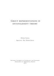
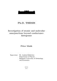
3. PARITY DEPENDENT SIMPLIFICATION AND APPROXIMATIONS 22Motivation of adding the two potentials comes from the fact that q(r) is written up asa sum for the L’s appearing. If minimal coupling is expected between the odd and evennumbered equations of the system of nonlinear equations the approximation has merit.3.4.2. T-set approximation (T). One may try to approximate the set of the shiftedangular momenta themselves. By unifying the two sets obtained by solving equations(2.78) and(2.79), onegets theT-set approximation T a = T e ∪T o . Usingthis approximateset T a in conjunction with equations (2.51), (2.49), and (2.26), one gets the approximateinverse potential V T (r). The motivation is the same as for the potential approximation(A), however the supposed minimal coupling is exploited at a different stage of thecalculation.3.4.3. One-term approximation (L). If the collision is dominated overwhelmingly bya single partial wave (as in the case of resonance scattering) then the equations (2.53)are to be solved at N = 1, and this results in the simple expression L = l − 2δ l /πfor the shifted angular momentum, assuming that the lth partial wave is dominating(δ l ∈ [− π 2 , π 2], see (2.100)). If however this is not the case, one still may try to use theapproximate expressions(2.91) L a = l−2δ l /πto form an approximate set T L . Using this approximate set T L in conjunction withequations (2.51), (2.49), and (2.26), one gets the approximate inverse potential denotedby V L (r). Thismostradical approximation, however, was applied alsowith somesuccess.3.4.4. An example: Gauss potential. For an exploratory analysis we prescribe a potentialof the Gauss form:(2.92) V G (r) = −2exp(−5r 2 )where both distance r and energy are measured in atomic units (au). Note, that wereturned to dimensionful quantities.Potential (2.92) provides a set of input phase shifts δ origllisted in table 2.1 at scatteringenergy of E = 18 au (k = 6 au). Using this input set one calculates the CT inversepotential V CT (r) = Eq CT (kr) which is depicted in figure 2.1. Note that V CT is the sameas V G within the width of line, therefore the plot of V G is omitted in figure 2.1.The different approximations V A , V L , and V T can thus be compared to V CT whichmay be taken to be exact. In figure 2.1 one can see that, for this particular example, thepotential V A (r) = Eq A (kr) is a good approximation to the original one in view of itsinitial behavior (depth) and asymptotic property (range). Recall that approximation V Ais obtained by simply adding inversion approximations V e and V o derived by invertingthe separate sets S e and S o of phase shifts belonging, respectively, to the sets of evenand odd angular momenta l ′ s. Approximation V T is obtained by unifying the calculatedsets T e and T o of shifted angular momenta, L ′ s, listed in table 2.1 under heading (2.78)or (2.79). Finally, the approximation V L has been obtained by simply using the onetermapproximate values L a , equation (2.91), which are also listed in table 2.1 underheading (2.91). It is interesting to see in figure 2.1 that this (totally analytical) version,the approximation V L provides a somewhat better result than that of the more involvedapproximation V T .

3. PARITY DEPENDENT SIMPLIFICATION AND APPROXIMATIONS 230.50.0V(r) (au)-0.5-1.0-1.5-2.00.0 0.2 0.4 0.6 0.8 1.0 1.2 1.4r (au)CTALTFigure 2.1. Inversepotentialsq(r)obtainedfrominputphaseshiftsδ origl(see table 2.1) as a function of the radial distance r at energy E = 18(k = 6) au. Curves obtained by the CT, and approximate methods arelabeled according to the procedures discussed in the text.Table 2.1. Original phase shifts δ origlproduced by the Gauss potential(2.92) at scattering energy E = 18 au. Shifted angular momenta Lcorrespondingtosolutionofequations(2.53), (2.78), or(2.79), and(2.91).l δ origl(2.53) (2.78) or (2.79) (2.91)0 0.1294 −0.0893 −0.0809 −0.08241 0.0964 0.9392 0.9391 0.93862 0.0535 1.9676 1.9666 1.96593 0.0232 2.9865 2.9861 2.98524 0.0082 3.9955 3.9954 3.99485 0.0025 4.9989 4.9989 4.99846 0.0006 5.9999 5.9999 5.99967 0.0001 7.0001 7.0001 6.99998 0.0000 8.0002 8.0002 8.00009 0.0000 9.0001 9.0001 9.000010 0.0000 10.0001 10.0001 10.0000

4. CONSISTENCY INVESTIGATIONS 244. Consistency investigations4.1. General condition. Asalreadyindicatedintheintroductionthekernelg(r,r ′ )only makes sense if the integral equation is uniquely solvable with it. As Eq. (2.25) canbe viewed as a Fredholm type integral equation of the second kind for fixed r, viz. ifrr ′ κ(r,r ′ ) = K(r,r ′ ) and rr ′ γ(r,r ′ ) = g(r,r ′ ) we have(2.93) κ(r,r ′ ) = γ(r,r ′ )−∫ r0γ(r ′ ,t)κ(r,t)dt.According to Fredholm’s alternative the Fredholm determinant thereof must be nonzerofor all fixed r > 0. When using the CT ansatz (2.45) the Fredholm determinant of theintegral equation becomes (to extent of a nonzero multiplicative term) the determinantof the system of the algebraic equations (2.51),{[uL (r)vl ′ (2.94) D(r) = det(r)−u′ L (r)v ] }l(r).l(l+1)−L(L+1)It is easy to see that for R ∈ Ω = {R : D(R) = 0, R ∈ R + } one gets∫ r(2.95) lim tq(t)dt = ±∞,r→R 0thus the potential is not in L 1,1 = {q : ∫ ∞0t|q(t)|dt < ∞}. While for Ω = ∅ we have[14](2.96)∫ ∞0tq(t)dt = ∑ L∈TlL∏l∈S (L−l)∏L≠L ′ ∈T (L−L′ ) < ∞.One can conclude the following Proposition [56], which (with some modificationsin the definition of D(r)) is valid for other procedures, where a second type Fredholmintegral equation is involved.Proposition 2. We get a unique solution of the GLM-type integral equation inC 2 (R + × R + ) and from that an inverse potential in L 1,1 = {q : ∫ ∞0t|q(t)|dt < ∞} ifand only if D(r) ≠ 0 on r > 0From [67] we know that D(r) ≠ 0 on r > 0 is not the case for arbitrary choice of Sand T: it was shown there, that if S = {0} and L = {2} then D(r) = 0 at some r > 0.With the help of Proposition 2 one can convince themselves that a particular CTinverse potential obtained numerically from arbitrary data is integrable or not. If it isintegrable then that potential will generate the input phase shifts.Also, using Proposition 2 it is possible to determine the admissible set of L numbersfor given l’s. In the one-l case we get a straightforward admissible set of L’s, however inhigher dimensions the formulation becomes extremely involved.4.2. One dimensional case. Inthiscase(S = {l}, |S| = 1)thefunctionW(u L ,v l )(r) ≡u L (r)vl ′(r) − u′ L (r)v l(r) must be examined carefully. The key idea of the proof is thatthe Wronskianu L (r)vl ′ (2.97)(r)−u′ L (r)v l(r)l(l+1)−L(L+1)

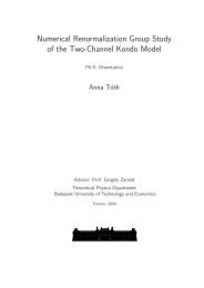
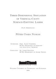
4. CONSISTENCY INVESTIGATIONS 25is nonzero on R + if and only if the constituent Bessel functions (J L+1/2 (r) and Y l+1/2 (r))are interlaced. This is deductible from the observation(2.98) D(r) = u L(r)vl ′(r)−u′ L (r)v ∫ rl(r)= u L (t)v l (t)t −2 dt.l(l+1)−L(L+1)The following gives the admissible set |l−L| ≤ 1.Theorem 1. W(u L ,v l )(r) has no roots on r ∈ R + , that is at N = 1 the GLM-typeequation is uniquely solvable for the CT method with S = {l} and T = {L} if and onlyif |L−l| ≤ 1. l ∈ (−0.5,∞), L ∈ (−0.5,∞) is supposed.Proof. The proof is trivial in light of Theorem 5 and Lemma 4 of Appendix B.Lemma 4 stipulates that W(u L ,v l )(r) has no roots on r ∈ R + iff J L+1/2 and Y l+1/2 areinterlaced. From Theorem 5 we infer that this is the case when 0 < |L−l| ≤ 1 which isexactly what we wanted to prove.□This result allows us to choose uniquely from the solutions(2.99) L = l− 2 π δ l +2n, n ∈ Z,of (2.53) at |S| = 1 as the solution for one input phase shift as(2.100) L = l− 2 [π δ l, δ l ∈ − π 2 , π ],2eliminating the ambiguity from the phase shift as well.At low energies it may happen that mostly only one partial wave contributes to thescattering amplitude (e.g. in case of resonances). It is worthwhile to look at the phaseshifts yielded by the CT inverse potential at the one-phase-shift level to get a sense ofthe quality of the inversion procedure.From Eq. (2.52) the following formula is inferred{0, l odd(2.101) tanδ l =L(L+1)L(L+1)−l(l+1) tanδ 0, l evenwhich specifies the phases of the CT potential for S = {0}. Note that it is a generalfeature that if phase shifts associated with only one kind of parity are specified for theinversion, then the phases of the CT potential with the opposite parity are exactly zero(see subsection 3.3).If e.g. the phase shift is restricted to describe an attractive potential (i. e. δ 0 > 0)the bound{0, l odd(2.102) 0 ≤ tanδ l ≤1tanδ4l 2 0 , l evencan be found using equation (2.101). This result assures the proper reproduction of thephase shifts by the CT potential.To illustrate these results figure 2.2 shows synthetic test potentials correspondingto l = 0, δ 0 = 0.2π obtained by the CT method. In addition to the L 1,1 potential aninconsistent one is also shown where n in equation (2.99) is chosen to be other than zero.As predicted we get a non-integrable potential.0

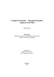
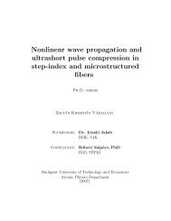
4. CONSISTENCY INVESTIGATIONS 26Figure 2.2. Potentials obtained by the CT method corresponding tol = 0, δ 0 = 0.2π with L = −0.4 (solid line) and L = 1.6 (dashed line).108IntegrableNon-integrable6q(r)420-20 2 4 6 8 10r4.3. Two dimensional case. Already in this case the Fredholm determinant becomescomplicated, which is also apparent from it’s integral representation(2.103) D(r) =∫ r ∫ r00u L1 (t)u L2 (s)(v l1 (t)v l2 (s)−v l1 (s)v l2 (t))t −2 s ′−2 dtds.Therefore instead of the analytical treatment we determine the admissible set of L’snumerically for some choices of l’s.Our numerical method was to check the determinant at the points of a fine latticeon the L 1 –L 2 quarter plane of (−0.5,∞)×(−0.5,∞) whether it has any zeros on (0,Λ),where Λ is a large number chosen to be great enough for(2.104) D(r > Λ) = const.+ε(r), |ε(r)| < εwith a very small ε. This can be done since every D(r) in any dimensions |S| < ∞ hasonly a finite number of zeros, because the constituent Wronskians all tend to constantsat large r distances, viz.[(2.105) W(r) = u L (r)v l ′ (r)−u′ L (r)v l(r) = cos (l−L) π ] ( 1+O , r → ∞.2 r)In figure 2.3 the admissible sets of {L 1 ,L 2 } pairs are depicted for the particularchoices S 1 = {1,3} and S 2 = {1,2}.In the next example (figure 2.4) we calculated some possible {L 1 ,L 2 } pairs for agiven {δ l1 ,δ l2 }. We note that only one of them is inside the permitted domain and couldonly find a single solution of the system of non-linear equation that is permitted by theconsistency condition. Again the L 1,1 and an inconsistent potential is shown.

4. CONSISTENCY INVESTIGATIONS 27Figure 2.3. The admissible sets of the T elements for (a) S 1 = {1,3}and (b) S 2 = {1,2} denoted by blank areas.(a)(b)Figure 2.4. Potentials obtained by the CT method corresponding toS = {0,1}, with phase shifts calculated from a Woods-Saxon potential.T = {−0.3056,0.9295} (solid line) and T = {1.0650,1.7016} (dashedline). Also, the original potential, q(r) = − [ 1+e 2.5·(r−1)] −1, yieldingthe phase shifts (δ 0 = 0.4389, δ 1 = 0.1246) is depicted (dotted line).1,00,80,60,40,2q(r)0,0-0,2-0,4-0,6-0,8IntegrableNon-integrableOriginal-1,00 2 4 6 8 10r

5. GENERALIZATION TO LONG-RANGE POTENTIALS 285. Generalization to long-range potentialsIn nuclear physics one frequently encounters charged particle scattering. Indeed itis the easiest experimental task to accelerate and guide charged particles. In this case,because of the long-ranged nature of the Coulomb interaction, the phase shifts do notdecay as fast as for short-range potentials and it would be inefficient to reconstruct along-ranged scattering potential from slowly decaying phase shifts. However one canalways change the reference potential from V (0) (r) = 0 to e.g. the Coulomb potentialand reconstruct the difference between the two by inverse scattering theory [61].It is convenient to reintroduce dimensionful quantities to treat the long-range extension.The reduced potential q DIM (r) = k 2 q(kr) will be used (the subscript shall besupressed) in the following and the dimensionless distance will be denoted by ρ withρ = kr.Consider a spherical potential q(r) which can be written as a sum of a short-rangeinterior (or nuclear) part ˆq(r) and a long-ranged exterior (asymptotic or reference) partq (0) (r), i.e.,(2.106) q(r) = ˆq(r)+q (0) (r).Then the phase shift itself is also split into two parts(2.107) δ l = ˆδ l +δ (0)lwhere δ (0)lis the phase shift due to q (0) and ˆδ l corresponds to the lth phase shift causedby ˆq in the presence of q (0) . If, for instance, ˆq(r) ≡ 0, ˆδ l = 0 ∀l.If the short-ranged part of the potential is zero beyond a finite distance r a ,(2.108) ˆq(r) = 0, r ≥ r athen, accordingly, the radial wave function can be written in this region as()(2.109) ψ l (k,r ≥ r a ) = C l F (0)l(kr)+tanˆδ l G (0)l(kr) .In the latter equation the functions F (0)land G (0)lare the regular and irregular solutionsof the dimensionless radial Schrödinger equation (1.4) with the dimensionless potentialk −2 q(k −1 r), respectively.Introduction of a reference potential can be carried out at two levels of the inversescattering calculation: at the level of the Schrödinger equation by designing a shortrangepotential which is in some sense equivalent to the original long-ranged potential,or at the level of the inverse procedure by using different reference functions.5.1. Phase transformation method. Whenpursuingthefirstpossibilityonegetsthe so called phase transformation method. In this case we introduce ˜q(r) which isidentical to the original potential (up to a constant energy shift) within the interiorregion 0 < r < r a and zero outside (see also Figure 2.5){q(r)−q(ra ), r ≤ r(2.110) ˜q(r) =a ,0, r ≥ r a .

5. GENERALIZATION TO LONG-RANGE POTENTIALS 29Figure 2.5. Depiction of the original potential q(r) and the one whosephaseshifts arecalculated by the phasetransformation method ˜q(r). Theregions U, A and Z refer to the unknown, the asymptotic and the zeroregions, respectively.q(r)20-2-4U-60,0 0,2 0,4 0,6 0,8 1,0r(a)Aq(r)0-2-4-6A ZU0,0 0,2 0,4 0,6 0,8 1,0r(b)If equation (2.108) holds true the ˆq interior potential can be deduced from ˜q. Theradial scattering wave function of this problem at the shifted ”energy” k 2 B = k2 −q(r a )is identical with the original one in the inside region(2.111) ˜ψl (k B ,r) = ψ l (k,r), r ≤ r abut differs in the outside region(2.112) ˜ψl (k B ,r) = ˜C)l(u l (k B r)−tan˜δ l v l (k B r) , r ≥ r a .The equality of the logarithmic derivatives at r = r a( )∣d 1(2.113)dr log r ˜ψ∣∣∣r=ral (k B ,r) = d ( 1dr log r ψ l(k,r))∣∣∣∣r=rawith ψ l (k,r) from (2.109) gives the transformed phase shifts ˜δ l (k B ) which can be usedto (re)construct the short-ranged potential Ṽ(r) (2.110). To get the original potentialone simply adds the reference potential{(2.114) ˜q (0) q(ra ), r ≤ r(r) =a ,q (0) (r), r ≥ r a .However equation (2.108) cannot hold when ˆq is reconstructed by a Newton-type methodsince the reconstructed potential in general decays as a second inverse power of thedistance. Therefore when using the phase transformation method one always introducesa small error.The phase shift transformation method has been introduced by May, Münchow andScheid [49] and was widely applied in case of the modified Newton Sabatier method(mNS). It was also applied to the CT inverse procedure to treat Coulomb scattering[50]. The author applied it to find proton–alpha effective scattering potential in [61].We shall term the CT procedure combined with phase transformation the PCT method.

5. GENERALIZATION TO LONG-RANGE POTENTIALS 305.2. Generalized CT scheme. If one pursues the second alternative of the referencepotential method one can derive a generalized CT (gCT) scheme which employsthe given nuclear phase shifts {ˆδ l } for constructing the short-range (nuclear) potentialˆq(r) but avoids use of a matching radius r a . The derivation starts with the ansatz forthe input symmetrical kernel of the Gel’fand-Levitan-type integral equation(2.115) g(ρ,ρ ′ ) = ∑ l∈Sγ l F (0)l(min(ρ,ρ ′ ))G (0)l(max(ρ,ρ ′ )),Then, by proceeding through the usual steps [4, 51], one arrives at a system of nonlinearequations identical in structure to (2.53)(2.116) e 2iˆδ l= 1+iK+ l1−iK − lor tan(ˆδ l ) =K + l+K − l2+i(K + l−K − l),l ∈ S,with(2.117) K ± l= ∑L∈T,l ′ ∈S[M sin ] lL [M −1[ ]cos] Ll ′e ±i (l−l ′ )π/2+δ (0)l ′ −δ (0)l, l ∈ S,and(2.118){MsinM cos}lL=⎧1⎨L(L+1)−l(l +1) ⎩(sincos(l−L) π 2 +δ(0) L −δ(0) l((l−L) π 2 +δ(0) L −δ(0) l))⎫⎬⎭ ,for the set T of the shifted angular momenta L where the relations S ∩ T = ∅ and|T| = |S| hold. From the set T one calculates the nuclear potential as(2.119) ˆq(r) = k 2 ς(kr),where(2.120) ς(ρ) = − 2 ( )d K(ρ,ρ)ρdρρwith(2.121) K(ρ,ρ ′ ) = ∑ L∈TA L (ρ)F (0)L (ρ′ ).The coefficient function A L (ρ) is calculated by solving the system of linear equations(2.122)∑L∈TA L (ρ) W[F(0) L (ρ),G(0) l(ρ)]l(l +1)−L(L+1) = G(0) l(ρ), l ∈ S,From this gCT scheme several developments are possible as the actual form of thereference potential has not yet been specified.

5. GENERALIZATION TO LONG-RANGE POTENTIALS 315.3. Coulomb reference potential method (CCT). If one sets the referencepotential to be the bare Coulomb potential(2.123) q (0) (r) = 2kηr≡ 1 Z 1 Z 2 e 2 2m4πε 0 r 2 ,with η being the Sommerfeld parameter then one arrives at the Coulomb CT (CCT)method. In this case the regular and irregular reference functions are the regular andirregular Coulomb wave functions, the reference phase shift is the Coulomb phase(2.124) σ l = 1 2i log [ Γ(l+1+iη)Γ(l+1−iη)], l ∈ S.Here it should be mentioned that in the course of application of CCT method itmay become necessary to know the regular and irregular Coulomb wave functions andCoulomb phases for complex orders. For example, in case of non-elastic scattering thephases are complex and therefore as noted before, the L numbers are also complexvalued. The Coulomb wave functions are well-defined for complex orders and similarlyto the real order case they can be given as power series (for details see Appendix B).It is interesting that contrary to the fact that the asymptotic forms of the referencefunctions contain the well known logarithmic term −ηln2ρ in the argument, it does notappear in the gCT formulas because of cancellation.Using the known power series of the Coulomb wave functions it can be shown thatthe CCT method gives a potential which is proportional to the Coulomb potential nearthe origin. For one term, i.e. |T| = |S| = 1, we get(2.125) q(r ≈ 0) = 2kηrFor large r we get(2.126) q(r → ∞) = 2kηr− 2 ∑∑r 2L∈T l∈S[ L(1+l)l(1+L)[M −1]+O(1).( ) 1cos] Ll cos(Θ L (kr)+Θ l (kr))+Or 3 ,with the Coulomb argument Θ L (ρ) = ρ−ηln2ρ−L π 2 +σ L.We see that the CCT method generates an inverse potential that gives a Coulomblikesingularity at the origin and produces a damped oscillation around the Coulomb tailat large distances. It is free of the matching parameter r a and requires just the nuclearphase shifts ˆδ l which are derived by usual phase shift analysis procedures.5.4. Modified Coulomb reference potential method (MCT). In order toobtain an inverse potential that is finite at the origin, instead of being singular there,we can modify the Coulomb reference potential accordingly. This reference potential isconstant in the interior domain and purely Coulombic outside. This modified Coulombpotential is the same as that employed by the phase transformation method for Coulombasymptotics and reads as(2.127) q (0) (r) ={2kηr a, r ≤ r a ,2kηr , r ≥ r a.

5. GENERALIZATION TO LONG-RANGE POTENTIALS 32To this reference potential there belong the following regular and irregular radial wavefunction⎧ (√ )⎨F (0) u l 1− 2ηkrl(ρ) =a ·ρ , r < r a ,(2.128)⎩ α (0) FF l (ρ)+β (0)l FG l (ρ), r > r a ,l⎧ (√ )⎨G (0) v l 1− 2ηkrl(ρ) =a·ρ , r < r a ,(2.129)⎩ α (0) GF l (ρ)+β (0)l GG l (ρ), r > r a ,land reference phase shift(2.130) δ (0)l= σ l +arctan( )βF (0)l.α (0) F lThe coefficients α (0) F,β (0)l F,α (0)l G,β (0)l Gcan be calculated from the equality of the innerland outer wave functions and their derivatives at the matching radius r a . The twocoefficients necessary for calculating the reference phase shift are(2.131) α F(0)l(2.132) β F(0)l==(√ )u l 1− ρa·ρa 2ηG l (ρ a)−√1− 2ηρa u′ l(√1− 2ηρa·ρa )G ′ l (ρa)F l (ρ a)G l (ρ − F′ l (ρa) ,a) G ′ l (ρa)(√ ) √ (√ )u l 1− ρa·ρa 2η 1− 2ηρaF l (ρ a)−u′ l 1− 2ηρa·ρaF l ′(ρa)G l (ρ a)F l (ρ − G′ l (ρa) ,a) F l ′(ρa)withρ a = kr a . Theother two coefficients areobtained byexchanging theregularRiccati-Bessel functions to the irregular ones.The total phase shifts can be written in two different ways(2.133) δ l = ˆδ l +σ l = δ MCTl +δ (0)lwhere ˆδ l means the nuclear phase shifts given as data and δlMCT is to be used to performthe CT inverse calculation outlined above.The potential obtained by the MCT method has a finite value at the origin. Becausethis method employs a similar reference potential as the PCT method, the results providedby the two methods should also be very similar, although quite different functionsare employed in the calculations. The advantage of the MCT over the PCT lies in thefact that it does not involve the small error in the phase shift reproduction inherent tothe PCT.5.5. An example. To illustrate the applicability of the long-range CT inversionprocedures we shall now use them to reconstruct model potentials. We model the α –α scattering with two slightly different potentials: the first is finite at the origin andthe second is singular (describing a possible non-locality). Let us also reintroduce thedimensional, physical potential V(r) = 22m q (DIM)(r).

5. GENERALIZATION TO LONG-RANGE POTENTIALS 33The first model potential is given by(2.134) V(r) = U(r)+V C (r),where the nuclear interaction is described by a Woods-Saxon [84] form( ) −1,(2.135) U(r) = U 0 1+e r−Raand the Coulomb interaction is represented by the potential of a homogeneous chargedsphere as{ ( )Z1 Z 2 e 2(2.136) V C (r) =2R C3− r2 , r ≤ RR 2 C ,CZ 1 Z 2 e 2r, r > R C .For the various parameters we choose the following values: Z 1 = 2, Z 2 = 2, A 1 = 4,A 2 = 4, U 0 = −20 MeV, R = R C = 2.0636 fm, a = 0.25 fm.The nuclear phase shifts ˆδ l were calculated at the center of mass energy E c.m. = 25MeV (see table 2.2). These phase shifts were then used as input data for the various CTcalculations. The results for the L-values are shown in table 2.2 and the correspondingpotentials are displayed in figure 2.6.Table 2.2. Model data (ˆδ origlphase shifts), inversion results (L shiftedangular momenta and ∆ˆδ l differences between the model phase shiftsand the ones given by the various methods‡) of the α – α scattering atE c.m. = 25 MeV. The matching parameter used in the PCT and MCTprocedureswassettor a = 10fm. NotethatthePCTandMCTpotentialscoincide.l L CCT L MCT LPCT ˆδorigl∆ˆδ CCTl∆ˆδ MCTl∆ˆδ PCTl0 −1.5622 −0.9225 −0.9219 1.2989 0.0085 0.0053 0.00561 0.5286 0.5841 0.5843 1.1445 0.0011 0.0009 0.00012 1.6462 1.7503 1.7502 0.8307 0.0116 0.0063 0.00623 2.9468 3.0281 3.0281 0.2300 0.0131 0.0025 0.00244 4.0456 4.1114 4.1115 0.0399 0.0176 0.0053 0.00545 5.0272 5.0983 5.0982 0.0062 0.0080 0.0019 0.00186 6.0308 6.0874 6.0875 0.0009 0.0073 0.0004 0.00057 7.0169 7.0684 7.0684 0.0001 0.0047 0.0039 0.00398 8.0177 8.0557 8.0557 0.0000 0.0001 0.0066 0.00669 9.0108 9.0428 9.0427 0.0000 0.0001 0.0108 0.0108‡ Note that for the sake of comparison the phases given by the inverse potentials werecalculated by cutting-off the non-physical oscillations beyond the matching radius r aused in the PCT procedure. Without the cut-off the MCT and CCT potentialsreproduce the phase shifts within an error of the numerical precision.One can observe that as expected the PCT and MCT procedures give almost thesame results and the CCT inverse potential is divergent at the origin.

5. GENERALIZATION TO LONG-RANGE POTENTIALS 34The second model is obtained by adding the singular potential term(2.137) V sing (r) = e−rr 2to the previous model, i.e.,(2.138) V(r) = U(r)+V C (r)+V sing (r).The reconstruction of phases is listed in table 2.3 and the potentials are shown in figure2.7. We see that the CCT potential follows nicely the model potential in the singulardomain near the origin while the PCT and MCT methods are unable to reproduce thesingularity although their phase shift reconstruction is good.Note that the reconstructions are not perfect which can be attributed to that onlya finite number of phase shifts were employed.Figure 2.6. Model potential (2.134) and inverse potentials yielded bythe CCT, MCT and PCT methods (labeled accordingly) at E c.m. = 25MeV center of mass energy. The model potential is non-singular at theorigin. (The PCT and MCT potentials coincide again.)840V(r) (MeV)-4-8-12CCTMCT-16PCTModel-200 1 2 3 4 5 6r (fm)

5. GENERALIZATION TO LONG-RANGE POTENTIALS 35Table 2.3. Model data and inversion results for the divergent modelpotential at E c.m. = 25 MeV. The matching parameter used in the PCTand MCT procedures was set to r a = 10 fm.l L CCT L MCT LPCT ˆδorigl∆ˆδ CCTl∆ˆδ MCTl∆ˆδ PCTl0 −1.5257 −0.8526 −0.8522 1.2121 0.0046 0.0038 0.00411 0.5116 0.5862 0.5862 1.1314 0.0011 0.0003 0.00072 1.6606 1.7506 1.7505 0.8245 0.0051 0.0043 0.00423 2.9505 3.0290 3.0290 0.2284 0.0061 0.0028 0.00274 4.0401 4.1108 4.1109 0.0395 0.0094 0.0060 0.00605 5.0293 5.0978 5.0977 0.0060 0.0036 0.0013 0.00136 6.0283 6.0870 6.0871 0.0008 0.0040 0.0031 0.00317 7.0179 7.0677 7.0677 0.0001 0.0030 0.0023 0.00238 8.0163 8.0553 8.0553 0.0000 0.0001 0.0008 0.00089 9.0113 9.0413 9.0413 0.0000 0.0020 0.0020 0.002010 10.0105 10.0325 10.0325 0.0000 0.0031 0.0024 0.002511 11.0077 11.0224 11.0224 0.0000 0.0018 0.0019 0.001912 12.0073 12.0155 12.0155 0.0000 0.0008 0.0014 0.001413 13.0056 13.0093 13.0093 0.0000 0.0005 0.0010 0.001014 14.0053 14.0065 14.0066 0.0000 0.0003 0.0006 0.000615 15.0043 15.0044 15.0043 0.0000 0.0002 0.0003 0.0003Figure 2.7. Model potential (2.138) and inverse potentials yielded bythe CCT, MCT and PCT methods (labeled accordingly) at E c.m. = 25MeV center of mass energy. The model potential is singular at the origin.840V(r) (MeV)-4-8-12-16CCTMCTPCTModel-200 1 2 3 4 5 6r (fm)

CHAPTER 3Transformational procedures1. IntroductionIn [27] it was shown that a subset of the fixed energy phase shifts, whose indexessatisfy the Müntz-Szász condition, determines the m-function and thus the spectralfunction, and thereby the potential of an auxiliary inverse spectral problem. Based onthis proof a constructive method was suggested in [28] for the solution of the inversescattering problem at fixed energy (in the following referred to as Horváth-Apagyi (HA)method).In this chapter first we examine the possibility of finding a suitable auxiliary inversespectral problem. Then, generalization of the method of Horváth and Apagyi is given[59] and a new approach is developed as well [60].It turns out that we need to transform the fixed energy radial Schrödinger equationto the Liouville normal form, which is unique to the extent of a scale parameter (c).The constructive methods considered for the recovery of the potential from scatteringdata are the Gel’fand-Levitan and the Marchenko inversions. In both procedures onehas the freedom to choose the boundary conditions which choice can be characterizedby a further parameter (h).Themostdifficultproblemofboundstates intheauxiliaryformalismisalsodiscussedto some extent. For the HA method an arbitrary number of boundstates are considered.Reduction of thenumberofboundstates isalso possiblebymakinguseoftheparameters(c and h). An approximative argument is presented to assess the number of boundstatespresent in the auxiliary problem.In this chapter we shall strongly rely on the results of the inverse spectral theory ofthe the Sturm-Liouville equation [38, 39, 16]. The necessary concepts and results arecollected in Appendix A.2. Liouville transformationFirst the fixed energy problem is transformed to an inverse eigenvalue problem wherethe value of the m-function for some arguments is determined from the original fixedenergy phase shifts. To this end we transform the radial Schrödinger equation[ ](3.1) r 2 − d2dr 2 +q(r)−1 ψ l (r) = −l(l+1)ψ l (r)to the Liouville normal form (see e.g. [10]) by using a Liouville transformation,(3.2) r → x(r), ψ l (r) → ϕ l (x).36

[ ẍ(3.3) −ϕ ′′l (x)− (x)ẋ 2 +2f′ f(x)2. LIOUVILLE TRANSFORMATION 37Rewriting the differential equation (3.1) in terms of the new independent variable x anddependent variable ϕ l (x) = f(x) −1 ψ l (r(x)) yields]ϕ ′ l (x)[ q(r(x))−1+ẋ 2− ẍ f ′ ](x)ẋ 2 f(x) − f′′ (x)f(x)l(l +1)ϕ l (x) = −r(x) 2 ẋ 2ϕ l(x)where dot denotes differentiation with respect to r. To get the Liouville normal form ofthe Sturm-Liouville equation we need(3.4) r(x) 2 ẋ 2 = const. = c 2 ,and(3.5)[ ] ẍ (x)ẋ 2 +2f′ ≡ 0.f(x)The two conditions yield the unique solution(3.6) x(r) = clogr +c 1and(3.7) f(x) = c 2 e x 2c .If we want to use the inverse spectral theory of the Sturm-Liouville equation on (0,∞)we need x(0) = +∞ and x(a) = 0 which in turn implies(3.8) sgnc = −1, c 1 = −cloga.Without the loss of generality c 2 = 1 is set and then the only remaining parameter c canbe chosen arbitrarily maintaining the negative sign.In summary, we have only one family of Liouville transformations reducingthe radialSchrödinger equation (3.1) to the Liouville normal form, namely(3.9) x(r) = clog r a , c < 0,(3.10)ϕ l (x) = e − x 2c ψl (ae x c ).Thereby (3.1) transforms to(3.11) −ϕ ′′l (x)+Q(x)ϕ l(x) = − 1 c 2 (l+ 1 2) 2ϕ l (x),with the auxiliary potential(3.12) Q(x) = a2c 2e2x cThe transformed equation can be viewed as( )q(ae x c)−1 .(3.13) S[Q(x)]y(x,λ) = λy(x,λ), S[Q(x)] = − d2dx 2 +Q(x)given explicitly at(3.14) λ = − 1 (c 2 l+ 1 ) 22

3. USING THE GEL’FAND-LEVITAN INVERSION – HORVÁTH-APAGYI METHOD 38also obtaining one of the two linearly independent solutions of the Sturm-Liouville equationas(3.15) y(x,− 1 (c 2 l+ 1 ) ) 2= ϕ l (x).2(Later we show that this is an L 2 solution.)2.1. m-function of the operator S[Q(x)]. First we show that for the previouslydefined Q(x), Q(x) ∈ L 1 (0,∞) holds:(3.16)∫ ∞0|Q(x)|dx ≤ 1 c 2 ∫ a∫ a0r 2 |q(r)|dr + a22|c| < ∞by the assumption q(r) ∈ L 1,1 (0,a).0 r2 |q(r)|dr < a ∫ a0r|q(r)|dr and c < 0 was alsoused. Then S[Q(x)] with Q(x) being the auxiliary potential is in the limit-point case(see Appendix A).Next we prove that the {ϕ l (x)} l=0,1,... functions are of the class L 2 (0,∞):(3.17)∫ ∞0|ϕ l (x)| 2 dx =∫ ∞0e −x c|ψ l (ae x c)| 2 dx = a|c|∫ a0|ψ l (r)| 2r 2 dr < ∞,where l ≥ 0 was exploited and the asymptotic formula ψ(r) = Cr l+1 (1 +o(1)), r → 0coming from equation (3.18) was used to estimate the integral.Since ϕ l (x) ∈ L 2 (0,∞), Q(x) ∈ L 1 (0,∞) and for compactly supported potentialsq(r) the wave function of the Schrödinger equation satisfies(3.18)(3.19)we infer that(3.20) mψ l (r) = C l r l+1 (1+o(1)), r → 0,ψ l (r) = A l√ r(Jl+1/2 (kr)−tanδ l Y l+1/2 (kr) ) , r ≥ a,) (− (l+1/2)2c 2 = ϕ′ l (0)ϕ l (0) = a Jl+1/2 ′ (a)−tanδ lYl+1/2 ′ (a)c J l+1/2 (a)−tanδ l Y l+1/2 (a) .Thus we have the m-function of the Sturm-Liouville operator S[Q(x)] with the potential(3.12) defined on the half-line.3. Using the Gel’fand-Levitan inversion – Horváth-Apagyi methodIn this section we use the Gel’fand-Levitan (GL) inversion procedure to find thetransformed potential Q(x). In order to complete this task we shall not use the explicitform of spectral functionas it wouldrequiretheapproximation of them-function, rather,in terms of the given m-function values, a moment problem is introduced for the inputfunction F(x) of the GL integral equation. Solving this moment problem proved to be,in this case, a numerically stable task contrary to the procedure consisting of the stepsof approximating the m-function from the given data, calculating the spectral functionand then solving the GL integral equation.Let us use the spectral problem ofSy = λy,whose elements are discussed in Appendix A.y(0) = 1, y ′ (0) = h < ∞

3. USING THE GEL’FAND-LEVITAN INVERSION – HORVÁTH-APAGYI METHOD 393.1. Deriving a moment problem. With referencetothedefiningformula(A.43)for F(x) we define a truncated version ˜F(x):∫ ∞(3.21) ˜F(x) = cos( √ λx)dσ h (λ).0It turns out that the reconstruction of the ˜F(x) function from the given m-functionvalues is an inverse moment problem. Consider∫ ∞∫ ∞(3.22) I = ˜F(x)e (l+1 2) x c dx =00(3.23)= − 1 c∫ ∞0∫ ∞0dσ h (λ)dxcos( √ λx)e (l+1 2) x c =dσ h (λ)l+ 1 2( )1c l+1 2.2 2 +λThis integration can be performed in terms of the m-function and by considering thaton (−∞,0) dρ h (λ) is concentrated on points (that is on the bound state eigenvaluesλ 1 λ 2 ,...λ B supported by Q(x)):(3.24)HereI = 1 c= 1 c(l+ 1 )·2(l+ 1 )2[ ∫ ∞⎡· ⎣−∞(md(ρ h (λ)−ρ 0,0 (λ))− 1 ( )c l+1 2+2 2 −λ1− 1 c 2 (l+12) ) 2−−h(3.25) b i = ρ h (λ i +0)−ρ h (λ i −0)∫ 0−∞]dρ h (λ)) 2 +λ(1c l+12 21m 0(− 1 (c l+12 2B∑+i=1) 2)b i(1c l+12 2) 2 +λi]and m 0 (·) denotes the m-function associated with Q(x) ≡ 0. The necessary values ofm(·) are known from equation (3.20).Now we have the following problem for ˜F(x):(3.26)∫ ∞with the moments(3.27) µ(c,h,δ l ,{λ i },{b i }) =0˜F(x)e (l+1 2) x c dx = µ(c,h,δl ,{λ i },{b i }), l = 0,1,...(l+ 1 ) (· a· J′ l+1/2 (a)−tanδ lYl+1/2 ′ (a) ) −12 J l+1/2 (a)−tanδ l Y l+1/2 (a) −c·h −1B∑ b i( )+ c l+12( )1i=1 c l+1 2.2 2 +λiNote that if there are no bound states supported by Q(x) the moments do not dependon the undetermined quantities {λ i } and {b i } associated with the bound state positionsand norms (last term of (3.27))..

3. USING THE GEL’FAND-LEVITAN INVERSION – HORVÁTH-APAGYI METHOD 403.2. Solution method. Depending on the number of bound states present in theauxiliary problem, different solution strategies are called for. As a consequence it isimportant to know or at least assess the number of bound states before solving theinverse problem which is discussed in the next section.3.2.1. No bound states. In this case we have a proper moment problem for ˜F(x) =F(x):(3.28)∫ ∞0F(x)e (l+1 2) x c dx = µ(c,h,δl ) ≡ µ l ,where the moments now do not depend on unknown quantities.To solve this moment problem we use the following expansion for F(x):(3.29) F(x) =N∑c n e −nx .n=0Upon substitution into equation (3.28) and usingN+1 fixed energy phaseshifts as inputdata we get the following system of linear equations for the coefficients(3.30)N∑n=0c n−c−cn+l+ 1 2= µ l , l = 0,1,...,N.Solving this system of linear equations yields the coefficients required to build F(x)and from that one can calculate the fixed energy potential essentially by solving theGL integral equation (A.41). Note that solving the system of equations is not a wellconditionedtask as we must deal with a Hilbert-type matrix which is infamously badlyconditioned. Therefore, from the numerical point of view it is of considerable value tosee, that this matrix can be inverted explicitly. Our matrix, i.e.[−c−cn+l+ 1 2]lnis in fact aCauchy matrix. The elements of the inverse of a general Cauchy matrix with elementsa ij = (x i +y j ) −1 are given by [74](3.31) b ij = (x j +y i ) ∏ m≠iIn our case this implies(3.32)c n = − 1 N∑cl=0x j +y m∏y m −y im≠j(µ l · l−cn+ 1 ) ∏ l −cn ′ + 1 ∏22 cn−cn ′ n ′ ≠n l ′ ≠lx m +y ix m −x j.l ′ −cn+ 1 2l ′ , n = 0,1,...,N.−lImprovements of the solution method. To further improve the solution method outlinedabove one can exploit two properties of the F(x) function, namely that(3.33) F(0) = −hand(3.34) lim F(x) = 0.x→∞

3. USING THE GEL’FAND-LEVITAN INVERSION – HORVÁTH-APAGYI METHOD 41The latter is a simple consequence of the Riemann-Lebesgue lemma, however the formerneeds more explanation. Let us write up the definition of F(0)∫ ∞ ∫ Λ[F(0) = dσ(λ) = lim dσ(λ) = lim ρ h (Λ)−ρ h (−∞)− 2 ]√Λ =−∞ Λ→∞ −∞ Λ→∞ π2= lim Λ+ρΛ→∞[π√ h (−∞)−h+o(1)−ρ h (−∞)− 2 ]√(3.35)Λ = −hπwhere equation (A.9) was used and continuity in Λ was supposed. This proves F(0) =−h.Because of F(∞) = 0 one can take(3.36) c 0 = 0;however, we note that this is not always the best course of action in practical scenarios(see later).To incorporate the information F(0) = −h there are several ways to choose from.For instance, one can prescribe the condition(3.37)N∑c n = −hn=0for the coefficients (which complicates the solution process: the matrix to be invertedis no longer of the Cauchy type). On the other hand, this will be very useful in theone bound state case (see later) where it will permit the determination of the nonlinearparameter λ in a linear way.Hausdorff moment problem. Our problem can be viewed as a Hausdorff momentproblem since with z = e x c and F(z) = −cz −1/2 F(clogz) (3.28) takes the form(3.38)∫ 10z l F(z)dz = µ l , l = 0,1,2,....The Hausdorff moment problem is studied in the literature in detail concerning bothmathematical properties and solution methods. For instance, an interesting stabilityresult can be found in [77] whose corollary is the following theorem, that establishes anaccuracy estimate of the inverse moment problem which is procedure independent.(3.39)Theorem 2. Suppose the smoothness condition∫ 10|F ′ (z)−F ′ N(z)| 2 dz ≤ E 2 < ∞.Then, if the first N +1 moments of F(z) and F N (z) coincide, i.e.(3.40)we have(3.41)∫ 10z k F(z)dz =∫ 10∫ 10z k F N (z)dz,|F(z)−F N (z)| 2 dz ≤k = 0,1,...N,E 24(N +1) 2.

3. USING THE GEL’FAND-LEVITAN INVERSION – HORVÁTH-APAGYI METHOD 42Using Theorem 2 one can conclude that if the moments µ l are free of error, thedifference between the approximated and the true F(x) functions in L 2 norm tends to 0as the number of moments is increased:(3.42)∫ ∞0|F(x)−F N (x)| 2 dx ≤C4(N +1) 2,with some C constant depending on the smoothness of F(x)−F N (x),(3.43)∫ ∞0|F ′ (x)−F ′ N (x)|2 e −2x c dx ≤ C,and F N (x) is the approximation of the true F(x) using the first N +1 moments.It is interesting to consider the case when the input data is noisy. Using Theorem 1of [77] one has the following estimate:(3.44)∫ ∞0{ ε|F(x)−F N (x)| 2 2dx ≤ minn |c| e3.5(n+1) +}C4(n+1) 2 : n = 0,1,...N ,where ε 2 is the absolute square sum of the differences between the true and noisy moments.This result implies in particular that even if the number of phase shifts grows toinfinity the recovery will not be complete when the data remains erroneous.3.2.2. One bound state. Supposing (3.29) we get the system of equations(3.45)N∑n=0c n−c−cn+l+ 1 2= µ l + b( l+ 1 12)c( )1c l+1 2, l = 0,1,...,N +1,2 2 +λwhere µ l denotes the lth moment without the bound state contributions and λ < 0 andb > 0 are the bound state parameters (the subscript 1 is omitted). Using the expansion(3.29) for ˜F(x) we have(3.46) F(x) = bcosh( √ −λx)+N∑c n e −nx .To get an explicitly solvable system of equations treating √ −λ as a parameter we subtractthe term b 2 e−√ −λx from the expansion for ˜F(x), that is prescribe∑N(3.47) ˜F(x) = c n e −nx − b 2 e−√ −λx , F(x) = b √2 e −λx+and obtain(3.48)n=0−c·b2( ( l+ 1 ) √ +2 +c −λ)through the elementary identity(3.49)N∑n=0c n−c−cn+l+ 1 2n=0N∑c n e −nx ,n=0= µ l , l = 0,1,...,N +1αα 2 −β 2 − 1 12(α+β) = 1 1, α,β ∈ C.2α−β

3. USING THE GEL’FAND-LEVITAN INVERSION – HORVÁTH-APAGYI METHOD 43Using the inverse of the Cauchy matrix the explicit solution of the system of equationsis given by(3.50)c n = − 1 cN+1∑l=0µ l(l −cn+ 1 )2 +cδ √n,−1 −λ× ∏ l ′ −cn+ 1 2 +cδ n,−1√−λl ′ −ll ′ ≠l× ∏ l−cn ′ + 1 2 +cδ n ,−1√ ′ −λ√ √ ,−cn ′ +cδ n ′ ,−1 −λ+cn−cδn,−1 −λn ′ ≠nwhere n = −1 is also allowed, c −1 ≡ b 2 and δ a,b is the Kronecker-delta. To determine√−λ we use a further result concerning Cauchy matrices, namely that the sum of thecoefficients (including b/2) is linear in √ −λ (see e.g. [28], Lemma 5):(3.51) S =N∑n=−1c n = α √ −λ+β.Using this fact the linear solution procedure is performed as follows.(3.52)(1) Calculate S for two arbitrarily chosen λ values (λ 01 and λ 02 ) solving (3.48).Denoting the two sums S 1 and S 2 , using the relation S = F(0) = −h get √ −λby√−λ =(S 2 +h) √ −λ 01 −(S 1 +h) √ −λ 02S 2 −S 1.(2) Calculate the c n coefficients from (3.48) with the appropriate λ parameter obtainedin (1).(3) Calculate q(r) through F(x) and the GL integral equation.3.2.3. Multiple bound states. For two or more bound states we propose a non-linearproblem. Firstly, solve the nonlinear system of equations(3.53)(3.54)∑ B −c·b ii=1+∑ N2(l+ 1 2 +c√ −λ i ) n=0 c −cn−cn+l+ 1 2∑ Bi=1 b i + ∑ Ni=0 c n = −h= µ l , l ∈ Lwith the index set L = [0,1,...,N+2B−1] in the variables λ 1 ,λ 2 ,...,λ B , b 1 ,b 2 ,...,b B ,c 0 ,c 1 ,...,c N . Then calculate F(x) by(3.55) F(x) =B∑i=1b i2 e√ −λ i x +N∑c n e −nxand finally solve the GL integral equation to obtain the potential.Numerically, it is worthwhile to initialize the c n values for the nonlinear solver withthe ones obtained for the known ka product supposing a q(r) ≡ 0 potential. Thisis because, roughly speaking, q(r) is expected to influence only the tail of the Q(x)potential and the bound states shall be close to those corresponding to q(r) ≡ 0.n=0

3. USING THE GEL’FAND-LEVITAN INVERSION – HORVÁTH-APAGYI METHOD 443.3. The constant potential and discussion of bound states. We shall makeobservations based on the transformation formula for the potential (3.12):(3.56) Q(x) = a2 ] [q(ae − |c|)−1x,c 2 e 2x|c|q(a) = 0.At most one bound state is expected when q(r) > 1 on 0 ≤ r < a, that is whenQ(x) is positive everywhere for h = 0 (Appendix A section 2.5). For instance an explicitexample is given by the case when we have a constant fixed-energy q(r) potential in theform(3.57) q(r) ={C for r < a0 for r ≥ a , C > 1.For such a potential it can be checked that there are no bound states (see later) forh = 0 and there is at most 1 bound state for h ≠ 0.Inpractical applications itisanaturalassumptionthatq(r) = 0already onb < r < awith some b > 0. In this case we have( ( a 2e−2(3.58) Q(x) = −c) x|c| b, 0 ≤ x < −|c|log ,a)only the tail of Q(x) is influenced by the fixed-energy potential q(r), e.g. Q(0) is solelydetermined by a. For this reason with given a parameter by taking q(r) ≡ 0 one cantry to calculate the approximate bound states or at least estimate the number of them.Next we show results for the constant potential, which covers the case of zero potential.For(3.59) Q(x) = −se −2tx , with s,t > 0the Sturm Liouville equation can be solved explicitly. This is an easy exercise and willnot be detailed here, only the result is given. The differential equation(3.60) −ϕ ′′ (x)−se −2tx ϕ(x) = λϕ(x)is solved by(3.61) ϕ(x) = C 1 J i√λ/t(√ st e−tx )+C 2 J −i√λ/t(√ st e−tx )where Bessel functions generally of complex orders have appeared. For Im √ λ > 0 theL 2 -solution (if t > 0) is(√ )(3.62) ϕ(x) = C 2 J √ s−i λ/tt e−tx ,since(3.63) J ±i√λ/t(√ st e−tx )= b(x)e ∓(Im√ λ/t)x +o(e ∓(Im√ λ/t)x ), x → ∞,where b(x) is some bounded function. Then the m-function is(3.64) m(λ) = ϕ′ (0) J ′ϕ(0) = −√ −i √ (√ s/t)λ/tsJ √−i λ/t( √ s/t) .

3. USING THE GEL’FAND-LEVITAN INVERSION – HORVÁTH-APAGYI METHOD 45Using the Stieltjes inversion, equation (A.17) dρ h (λ) can be found. For λ > 0 trivially(3.65) dρ h (λ) = 1 π Im [√s J ′ −i √ λ/t (√ s/t)J −i√λ/t( √ s/t) +h ] −1dλ, λ > 0.Forλ < 0themeasureisconcentrated topointswhicharetheboundstates. Theyarelocated at the eigenvalues of the operator where ϕ ∈ L 2 (0,∞). Starting from ϕ(0) = 1and ϕ ′ (0) = h one can calculate the coefficient of the divergent solution to be(3.66) C 1 = − π√ s2t[J ′ √ −λ/t( √ s/t)+ h √ sJ √ −λ/t (√ s/t)where some elementary properties of the Bessel functions were used [82]. C 1 needs tobe zero thus the bound states are located at λ’s which satisfy(3.67) J ′ √ −λ/t( √ s/t)+ h √ sJ √ −λ/t (√ s/t) = 0.Then the number of boundstates is greater than zero but finite. Note that for s < 0 (thecase of potential (3.57)), we have the modified Bessel function (i λ I λ (x) = J λ (ix)) and itsderivative in the previous equation at √ |s|/t ∈ R + , which functions are monotonicallyincreasing allowing at most one solution (bound state), while for h = 0 allowing none.Using the theory of residues the height of the step in ρ(λ) at the bound states canbe obtained to be(3.68) ρ(λ 0 +0)−ρ(λ 0 −0) = 2t √ J √ −λ−λ0 /t (√ s/t)√ (1,1) sJ √ −λ0 /t (√ s/t)+hJ √ (1,0)−λ0 /t (√ s/t) ,where the superscript (n,m) means derivation with respect to order n times and derivationwith respect to the variable m times.In case of h = 0 we have a particularly simple scenario at hand. For definiteness let(3.69) κ 2 = 1−q(0),q(0)beingthevalueoftheconstantpotentialate.g. theorigin, andsupposeforsimplicityq(0) < 1. The potential Q(x) = − (κa)2states λ i atc 2 e −2x(3.70) J ′ |c| √ −λ i(κa) = 0.|c|associated to q(r) ≡ 0 with h = 0 has boundFrom [82] we infer, denoting the nth root of J µ(x) ′ by j µ,n, ′ that j µ,n ′ < j µ+ε,n ′ n = 1,2,...holds with j 0,1 ′ = 0. Moreover, j′ µ,n is continuous in µ [82]; therefore, we find that forκa > 0 there always exits at least one bound state. From the above fact it also followsthat the number of zeros of J 0 ′ (x) on 0 ≤ x < κa equals the number of bound statesof Q(x) = − (κa)2 e −2x |c|. Alternatively, as J ′ c 2 0 (x) = −J 1(x), the number of bound statesincrease at the zeros of J 1 (x), i.e. at j 1,n , n = 1,2,.... Some numerical results are listedin Table 3.1. For a general potential q(r) the data listed in Table 3.1 can still be relevantif the potential is shallow compared to 1 and only the tail of Q(x) is influenced by q(r).Note that the value of the parameter c does not affect the number of bound states (onlytheir positions) as it is only a scale parameter of the function J ′ |c| √ −λ (κa) of √ −λ whosezeros give the bound states.]

3. USING THE GEL’FAND-LEVITAN INVERSION – HORVÁTH-APAGYI METHOD 46Table 3.1. The first few sectors of definite bound state numbers for aconstant q(r) potential at h = 0.0 < κa < 3.8317 one bound state3.8318 < κa < 7.0156 two bound states7.0156 < κa < 10.174 three bound states10.174 < κa < 13.324 four bound statesetc.Figure 3.1. J µ (κa) ′ (full line) and RJ µ (κa) (dashed line) as functionsof the order (R is a real number satisfying sgn(J 0 ′(κa)) = sgn(RJ 0(κa))and |RJ 0 (κa)| > |J 0 ′ (κa)|). While at h = 0 the zeros of the derivativefunctionsaretheboundstates, at h ≠ 0theintersection of thetwo graphsgive them.0.40.2J Μ Κa ′R J Μ Κa0.02 4 6 8 100.20.4Allowing h ≠ 0 gives rise to the more involved condition (3.67) with √ s = a|c|andt = |c| −1 for the bound states. It is possible then for some h ≠ 0 that one has one boundstate while for h = 0 two of them. This has the favorable consequence of reducinga nonlinear problem to a linear one. Without giving an exhaustive treatment of thesituation we show the following illustrative result for bound state reduction.Lemma 1. For 3.83 ≈ j ′ 0,2 < κa < j 0,2 ≈ 5.52 the two bound states present at h = 0can be reduced to one by varying h.Proof. In figure 3.1 the two Bessel-type functions entering condition (3.67) aredepicted. We will show that by varying h (on the figure through R), disregarding anoverall sign, one can always get the same kind of graphs as the ones on the figure andhave only one bound state.By using the fact that the zeros of J 0 (x) and J 0 ′(x) interlace we infer that J 0(κa) ≠ 0and J 0 ′ (κa) ≠ 0. The only thing that remains to be shown is that the distribution of

3. USING THE GEL’FAND-LEVITAN INVERSION – HORVÁTH-APAGYI METHOD 47the zeros are as depicted. Since j 0,2 ′ < κa < j 0,2 for J µ(κa) ′ only the first two andfor J µ (κa) only the first zeros can enter into our considerations. Then the interlacingrelation j a,1 ′ < j a,1 < j a,2 ′ and the monotonicity of the zeros translate into µ 1 < µ 2 < µ 3if j µ ′ 1 ,1 = κa, j µ 2 ,1 = κa and j µ ′ 3 ,2 = κa. This completes the proof of the lemma. □3.4. Examples.3.4.1. Constant potentials. First a potential that generates no bound states in theauxiliary problem is reconstructed. Let us take{1.2 for r < 2(3.71) q(r) =0 for r ≥ 2with a = 2. Note that q(0) = 1.2 > 1, therefore Q(x) > 0.Figure 3.2 1 shows how the quality of the inversion increases when the number ofinput phase shifts is increased: results are shown with 5, 10, 20 and 40 input phaseshifts using the parameters c = −0.8 and h = 0. In order to preclude the possibility oferrors introduced by inaccurate data and that of rounding errors (originating from thefact that we are dealing with severely ill-conditioned matrices that need to be inverted)we worked with a precision of a hundred digits.Figure 3.2. Reconstructions with different number of inputphase shiftsof the constant potential q(r) = 1.2·H 2 (r). (c = −0.8, h = 0.)qr1.401.351.301.251.201.151.101.051.00 0.0 0.5 1.0 1.5 2.0 r(a) 5 phases.qr1.401.351.301.251.201.151.101.051.00 0.0 0.5 1.0 1.5 2.0 r(b) 10 phases.qr1.401.351.301.251.201.151.101.051.00 0.0 0.5 1.0 1.5 2.0 r(c) 20 phases.qr1.401.351.301.251.201.151.101.051.00 0.0 0.5 1.0 1.5 2.0 r(d) 40 phases.1 For brevity we introduce the function Ha(x) being a step function: H a(x) = 1 for x ≤ a andH a(x) = 0 for x > a.

3. USING THE GEL’FAND-LEVITAN INVERSION – HORVÁTH-APAGYI METHOD 48Figure 3.3. Reconstructions of the constant potential q(r) = 1.2·H 2 (r)from 11 phase shifts with no bound states in the auxiliary problem usingthe parameters a = 2, c = −0.8, h = 0 (a) excluding, (b) including theconstant term in equation (3.29) .qr1.51.41.31.21.11.00.90.8 0.0 0.5 1.0 1.5 2.0 r(a) Without constant.qr1.51.41.31.21.11.00.90.8 0.0 0.5 1.0 1.5 2.0 r(b) With constant.An interesting feature is displayed in figure 3.3: it can be beneficial to retain theconstant term in the expansion (3.29) (while it is incompatible with the theoretical formof F(x)). The figure depicts the reconstruction of the previous potential with c = −0.8and h = 0. Motivated by this example in the reconstructions to be shown the constantterm is retained in the expansion, whose value will also serve as an overall measure ofthe quality of the inversion.Figure 3.4 shows inverse potentials generated from the same number N + 1 = 11of fixed energy phase shift data. By varying the parameters c and h one can achieveconsiderably better reconstructions thanwith theoriginal choices of parameters (c = −1,h = 0). In this case the optimal choice was c = −0.3 and h = −0.15.To make the choice of the parameter systematical, we introduce a measure of thesmoothness of the inverse potential: let∫ a(3.72) s(c,h) = |q ′ (r)|dr,r 0definedforeachchoiceofcandhwherethelower limitr 0 isintroducedinordertoexclude(possibly pathological) singularity at the origin. We used r 0 = 0.05 in all the examplesshown. By requiring s to be small is equivalent to prescribe smoothness of the potential.Also, such a potential cannot contain non-integrable parts, singularities (see Chapter 2,Section 3), which in principle could also be encountered in the HA method. Indeed, weonly have an approximation of the trueF(x) inputfunction for theGL integral equation,therefore it is possible that the integral equation has a vanishing Fredholm determinantfor some radii. In such a case the HA method becomes inconsistent as well, thus suchcases should be excluded from consideration outright. On the other hand, requiringsmooth potentials also means that we have an underlying smooth F-functions too, forwhich Theorem 2 implies better reconstruction, in principle.Next we show an example for a so called spurious bound state. Notice, that reconstructionof a potential with a procedure appropriate for more bound states thenare truly present in the auxiliary problem is possible and not inconsistent (while in the

3. USING THE GEL’FAND-LEVITAN INVERSION – HORVÁTH-APAGYI METHOD 49Figure 3.4. Reconstructions of the constant potential q(r) = 1.2·H 2 (r)from 11 phase shifts with no bound states in the auxiliary problem withdifferent choices of the parameters c and h.qr1.30qr1.301.251.251.201.201.151.151.10 0.0 0.5 1.0 1.5 2.0 r(a) c = −1, h = 0 (originalchoice). s=12.1.10 0.0 0.5 1.0 1.5 2.0 r(b) c = −1, h = −0.15. s=15.qr1.30qr1.301.251.251.201.201.151.151.10 0.0 0.5 1.0 1.5 2.0 r(c) c = −0.30, h = 0. s=0.15.1.10 0.0 0.5 1.0 1.5 2.0 r(d) c = −0.30, h =−0.15. s=011.opposite case it would be). For instance, for the test potential (3.71) allowing one nonlinearparameter √ −λ (a spurious bound state), the reconstruction results in the sameprecision as before without the inclusion of a ”bound state”. Results for c = −0.3 andh = −0.5 are depicted in figure 3.5 (together with the intermediate functions F(x) andQ(x)). In addition to the reconstructed potential we list the input phase shifts and theintermediate data (such as the moments, coefficients of the series (3.29) and the value ofthe ”bound state”) in Table 3.2. Typical features can be seen on the numbers appearing:while the phase shifts decrease exponentially, the moments µ l decrease only as a powerfunction (in general as l −1 ); the expansion coefficients are altering in sign to produce∑cn = h; c 0 is small. It is also worth pointing out that in this case the procedureyields √ −λ = −1.4447 for the ”bound state” parameter, a negative value which clearlyindicates that there is no real bound state in this problem. Thus, it could be a possiblecourse of action, one that in principle can yield the true number of bound states in theauxiliary problem, to reconstruct the potential, or at least calculate the bound statepositions with the B = 1,2,... procedures until one encounters a negative bound stateparameter. Then one can conclude, that the true number of bound states is one lessthen the B-value, where the algorithm stopped.

3. USING THE GEL’FAND-LEVITAN INVERSION – HORVÁTH-APAGYI METHOD 50Figure 3.5. (a) Reconstruction of the potential q(r) = 1.2·H 2 (r) withc = −0.3, h = −0.5 employing the one bound state procedure (see text).s = 0.0004. (b) Function F(x). (c) Potential Q(x) in the x-space.qr1.30Fx0.6Qx81.250.40.261.200.01 2 3 4 5 x41.151.10 0.0 0.5 1.0 1.5 2.0 r(a) q(r).0.20.40.6(b) F(x).20 0.0 0.5 1.0 1.5 2.0 x(c) Q(x).Table 3.2. Input phases (δ l ) and the intermediate quantities of the inversionprocedure: moments µ l , coefficients c n and the nonlinear parameter(i.e. ’bound state’). a Nonlinear ”bound state” parameter:√−λ = −1.4447.l δ l µ l n c n0 −0.9890 −0.1714 −1 −6.4667 a1 −0.2964 −0.0043 0 +0.00022 −0.0471 0.0151 1 −0.09543 −0.0037 0.0180 2 +7.20854 −0.0001 0.0176 3 −0.15105 −5.0×10 −6 0.0164 4 +0.26576 −1.1×10 −7 0.0151 5 −0.29687 −1.8×10 −9 0.0139 6 +0.20278 −2.2×10 −11 0.0129 7 −0.20229 −2.3×10 −13 0.0119 8 +0.025810 −1.9×10 −15 0.0111 9 +0.0092Now we proceed to reconstruct the potential{0.8 for r < 2 = a(3.73) q(r) =0 for r ≥ 2 = awhich possesses one bound state at h = 0 (since q(0) = 0.8 < 1, thus Q(x) < 0). Infigure 3.6 two potentials are shown with different choices of the parameters. Note thequality: for r > 0.5 the deviation from the original potential is in the order of 0.00010(s = 0.049) for c = −1, h = 0 and 0.00005 (s = 0.0022) for c = −0.5, h = −0.65.We continue with a two bound state potential at h = 0,{0.8 for r < 11 = a(3.74) q(r) =0 for r ≥ 11 = a.

3. USING THE GEL’FAND-LEVITAN INVERSION – HORVÁTH-APAGYI METHOD 51Figure 3.6. Reconstructions of the constant potential q(r) = 0.8H 2 (r)from 11 phase shifts and one bound state in the auxiliary problem ath = 0 with different choices of the parameters.qr0.810qr0.8100.8050.8050.8000.8000.7950.7950.790 0.0 0.5 1.0 1.5 2.0 r(a) c = −1.0, h = 0.0.790 0.0 0.5 1.0 1.5 2.0 r(b) c = −0.5, h = −0.65.Figure 3.7. Reconstructions of the potential q(r) = 0.8 · H 11 (r) using(a) the two bound state formulation (h = 0) and (b) the one bound stateone (h = 5). c = −1.5 was taken.qr0.810qr0.8100.8050.8050.8000.8000.7950.7950.7900 2 4 6 8 10(a) h = 0, two bound states.r0.7900 2 4 6 8 10(b) h = 5, one bound state.rIn figure 3.7a the reconstruction is depicted using two bound states in the inversionprocedure while in figure 3.7b reconstruction for h = 5 is shown where only one boundstate is present in the auxiliary problem. One can check that in this case κa ≈ 4.92 thusit is in the domain where the number of bound states can be reduced (Lemma 1).3.4.2. Potentials with different shapes. To depart from constant potentials we continueon to the piecewise constant potential⎧⎪⎨ 0.25 for r < 1(3.75) q(r) = 0.125 for 1 ≤ r < 2⎪⎩0 for 2 ≤ rwith a = 2. This potential is more complicated than the constant potentials while itsphase shifts can still be calculated exactly. The inversion results are shown in figure3.8. Note the relatively high number N + 1 = 31 of phase shifts required for the

3. USING THE GEL’FAND-LEVITAN INVERSION – HORVÁTH-APAGYI METHOD 52Figure 3.8. Reconstruction of the piecewise constant potential with differentchoices of theparameters. 31 phaseshifts wereusedwith aworkingprecision of 100 digits.qr0.4qr0.40.30.30.20.20.10.10.0 0.0 0.5 1.0 1.5 2.0 r(a) c = −1, h = 0.0.0 0.0 0.5 1.0 1.5 2.0 r(b) c = −1.4, h = −0.5.reasonable reconstructions shown in figure 3.8. And we still employed 100-digit data.This discouraging result is probably a result of the discontinuous nature of the potential.We also reconstructed (figure 3.9) a Gauss and a Woods-Saxon potential given by(3.76) q G (r) = −4e −5r2 , q WS (r) = −4(1+e r−0.50.1) −1,where the dimension of the reduced potentials has been restored and for the scatteringwavelength k = 1.5 was taken. In this case while the phase shifts are not known exactlyand were only calculated to a few digits of precision, the reconstruction is quite acceptable.In case of the Gauss potential the phase shifts were calculated to a precision offour digits (see table 3.3 also for the intermediate quantities) while for the Wood-Saxontype only to two (see table 3.4). For these potentials the bound state approximationprocedure is applicable and the prediction gave one bound state at λ = −3.22 for theGauss and also one bound state for the WS at λ = −2.44. The calculation resulted inλ = −3.36 and λ = −2.46, respectively, which figures are in good agreement with theones obtained from the approximation.Table 3.3. Input phases δ l and the intermediate quantities (µ l , c n ) ofthe inversion procedure for the Gauss potential.l δ l µ l n c n0 0.2322 −1.147 −1 +0.96501 0.0153 4.738 0 −0.62672 6.552×10 −4 0.4669 1 +2.6783 2.078×10 −5 0.2050 2 −6.4194 5.174×10 −7 0.1189 3 +5.9075 1.056×10 −8 0.0785 4 −3.0666 1.827×10 −10 0.0560 5 +0.562

3. USING THE GEL’FAND-LEVITAN INVERSION – HORVÁTH-APAGYI METHOD 53Table 3.4. Input phases δ l and the intermediate quantities (µ l , c n ) ofthe inversion procedure for the Woods-Saxon potential.l δ l µ l n c n0 0.37 −0.9597 −1 +0.76161 0.023 −2.2973 0 −0.00822 0.00087 1.5792 1 +0.08953 0.000026 0.4633 2 −0.8429Figure 3.9. Reconstruction of the dimensionful reduced Gaussian andWSpotentials from7phaseshiftsgivenwithprecisionof4digitsandfrom4 phase shifts given with 2 digits of precision at k = 1.5. The parameterswere a = 1.5, c = −0.74, h = 0 for the Gauss while a = 2, c = −1.25and h = 0 for the Woods-Saxon potential. The original potentials aredepicted with dashed while the reconstructions with solid line.qr0.5 1.0 1.5rqr00.5 1.0 1.5 2.0 r112234354(a) Gauss.(b) Woods-Saxon.

4. USING THE MARCHENKO INVERSION 544. Using the Marchenko inversionIn this section a new procedure is developed based on the Liouville transformationand using the Marchenko inversion with physical boundary condition,(3.77) y(0,λ) = 0,in the auxiliary problem.The Marchenko procedure involves the linear integral equation(3.78) F(x+y)+K(x,y)+∫ ∞xK(x,t)F(t+y)dt = 0, (x ≤ y)for the transformation kernel K(x,y). The input function F(x) reads(3.79) F(x) =B∑j=11e −λjx + 1 ∫ ∞ (1−e 2i∆(κ)) e iκx dκm j 2π −∞where the first term accounts for the bound states in the spectrum generated by Q(x)(B = 0, zero bound state is supposed), while the second is the scattering contribution(alsodenotedbyF S (x)). Theoddfunction∆(κ)intheintegralisthephaseshiftfunctioncorresponding to the transformed potential Q(x). In our inverse problem we have them-function at some points on the negative part of the real line as data.The method proposed here to get the potential from the m-function values consistsof(1) interpolation of the m-function and determination of the Jost-function from them-function,(2) use of the dispersion relations for the Jost function to get the phase function∆(κ) and(3) calculation of the input function from the phase function by (3.79) from whichthe Marchenko equation (3.78) readily yields the potential.4.1. Interpolation of the m-function. We shall use a consequence of Simon’srepresentation of the m-function [76, 24]: the m-function can be represented essentiallybyaLaplacetransform. ForboththeFourierandtheLaplacetransformsthereareknowninterpolation formulas, and the latter allows for the interpolation of the m-function [70].We have (as a special case of Theorem 5 of Ref. [70])(3.80) m(λ) ≈ i √ l∑maxλ+ c n (−i √ λ)with ω m = m+ 1 2 andn=0n∑a nm (m(−ωm 2 )+ω m)m=012(3.81) c n (x) = (2n+1)(( −x) n12 +x) , a nm = (−n) m(n+1) m(m!) 2 .n(x) n is the Pochhammer symbol:(3.82) (x) n = x(x+1)...(x+n−1), (x) 0 = 1.

4. USING THE MARCHENKO INVERSION 55The interpolation formula applies for locally absolute integrable potentials. Its domainofconvergence dependsonthespecificfeatures ofthepotential andwesupposeit tobe valid on the whole complex λ−plane throughout the subsequent numerical examples.4.2. Constructing the scattering data from the m-function. Because of theBorg-Marchenko theorem one might surmise that the m-function ”knows” the operatorcompletely. Thus it is expected that the scattering data (phase shifts, bound stateswith normalization – the building blocks of (3.79)) for any boundary condition can berecovered from it. It turns out that the phase shifts are deductible from m(λ + i0),λ ∈ R while the bound states correspond to poles of m(λ). Here, the case when thereare bound states supported by Q(x) is left as an open problem.The m-function and the Jost function are connected by the following formula (A.26)(3.83)|f + (κ)| 2κ= limε→0 + 1Im(κ 2 +iε) , κ > 0.This relation, however, only gives the absolute value of the Jost function. There is aformula connecting the argument (that is the phase function) and modulus of the Jostfunction called the dispersion relation [38]. For(3.84) f + (κ) = |f + (κ)|e i∆(κ)we have (due to analyticity)(3.85)∫Clogf + (κ ′ )dκ ′κ ′ −κand the C contour is given by {κ ′ ∈ Re iφ ,φ ∈ [0,π]}∪{κ ′ ∈ [−R,+R]}\{κ ′ ∈ [κ−ǫ,κ+ǫ]}∪{κ ′ ∈ ǫe iφ ,φ ∈ [π,0]} and R → ∞, ǫ → 0 if there are no bound states, that is nozeros of the Jost function or no poles of the integrand. Then the following holds(3.86) ∆(κ) = 1 π P ∫ ∞−∞= 0log|f + (κ ′ )|dκ ′κ ′ −κcalled the dispersion relation. P denotes that the integral is understood as a the Cauchyprincipal value integral.4.3. Marchenko equation. With the input function at hand one needs to solveequation (3.78) for K(x,y) which yields the potential(3.87) Q(x) = 2 ddx K(x,x).However, for better performance, we transform both the input function and theMarchenko equation back with the variable change r = ae −x . With the definitions(3.88) ˜K(r,r ′ ) ≡ K(−log r r′,−loga a ),(3.89)˜F(r,r ′ ) ≡ F(−log r r′−loga a )we arrive at the integral equation(3.90) ˜F(r,r ′ )+ ˜K(r,r ′ )+∫ r0˜K(r,r ′′ ) ˜F(r ′′ ,r ′ ) dr′′r ′′ = 0.

4. USING THE MARCHENKO INVERSION 56It is interesting to note that this equation is the one that arises when studying the fixedenergy inverse scattering problem without a Liouville transformation (see Chapter 2,section 1). Also, our transformed input kernel,(3.91) ˜F(r,r ′ ) = F(−log r a−logr′a)= F(−log rr′a 2 )is a function of rr ′ . However, what makes the present approach different is while in theframework presented at the beginning of Chapter 2 the fixed energy phase shifts areneeded for l ∈ R + ∪iR + , well in a nonphysical domain, the transformational approachrequires the physical phase shifts only (in agreement with the uniqueness theorem, andnecessary and (almost) sufficient condition, see Chapter 1, Section 2).For convenience we perform one further transformation on the input and transformationkernels. Let(3.92)¯K(r,r ′ ) ≡ ˜K(r,r ′ )√ ,rr ′(3.93)¯F(r,r ′ ) ≡ ˜F(r,r ′ )√ .rr ′Then the integral equation takes on the form(3.94) ¯F(r,r ′ )+ ¯K(r,r ′ )+∫ r0¯K(r,r ′′ ) ¯F(r ′′ ,r ′ )dr ′′ = 0,which is identical to the GL equation, only now in r-space. The fixed energy potential,q(r) is obtained by(3.95) q(r) = 2 rAlternatively,(3.96) q(r) = 2 rd˜K(r,r)dr+k 2 = 2 rd ( )r¯K(r,r) +k 2 .drdK(−log(r/a),−log(r/a))dr+k 2 .Tofirstorder,thesmall-r behaviourof ˜K(r,r)canbeextractedfrom ˜K(r,r) ≈ − ˜F(r,r) =−F(−2log(r/a)). Using asymptotic examination of F(x) it can beshown, that ˜K(r,r) ispolynomial in r as r → 0 since the asymptotic series of F(x) contain only exponentiallysmall terms. If the smallest absolute valued exponent µ in the asymptotic series of F(2x)(which could be extracted from the poles of ∆(κ), if it were known for arbitrary κ ∈ C)is µ ≥ 2, the resulting potential q(r) is finite at the origin. Our analysis indicated, thatµ is not universal, thus the behaviour of the inverse potential at the origin is neither.4.4. Numerical refinements. The accurate numerical calculation of the phasefunction is hindered by the fact that the Jost function falls off at infinity as an inversepower. Therefore we propose to extract at least the first term in the asymptotic seriesand perform the prescribed integral analytically for it.Supposing (see Lemma 2 below)(3.97) |f + (κ)| = 1+ β ( ) 1κ 2 +o κ 2 , κ → ∞

we get(3.98) ∆(κ) ≈ 1 π P ∫ M4. USING THE MARCHENKO INVERSION 57−Mlog|f + (κ ′ )|dκ ′κ ′ −κ− β ( 2πκ M + 1 )M −κlogκ M +κFor F S a similar extraction of the asymptotics is in order. First, let us recast F Sinto(3.99) F S (x) = 1 ∫ ∞(cos(κx)−cos(κx+2∆(κ)))dκ2π0by using the oddness of ∆(κ). Since the phase function is odd one can assume(3.100) ∆(κ) = α κ +O(κ−3 ), κ → ∞Then the contribution of the tail of the integrand is well approximated byT(A,x) ≡ 1 ∫ ∞(cos(κx)−cos(κx+2∆(κ)))dκ2π A(3.101)≈ α(αx−1) (2Si(Ax)−π)+ α22π πA cos(Ax))where Si(x) is the sine integral. Then F S (x) is to be calculated by∫ A(3.102) F S (x) ≈ 1 (cos(κx)−cos(κx+2∆(κ)))dκ+T(A,x)2π 0where the remaining integral is performed numerically.To conclude this section we prove (3.97).Lemma 2. For real valued potentials|f + (κ)| = 1+ β κ 2 +o ( 1κ 2 ).Proof. If Q(r) is real than the kernel K(x,t) is real (see (A.22)). Then, fromequation (A.21) we infer∫ ∞( ) 1f + (κ) = 1+2 K(0,t)cos(κt)dt+Oκ 2 , κ → ∞.0Using the stationary phase approximation for Fourier integrals [54] it is easy to see thata cos-Fourier transform of a regular, real function (with no singularities on [0,∞]) is atmost O ( )1κ as κ → ∞.□24.5. Examples.4.5.1. Constant potentials. To the fixed energy potential{q 0 for r ≤ a(3.103) q(r) =0 for r > abelongs the transformed potential(3.104) Q(x) = −se −2x , s = a 2 (1−q 0 ).The general solution of the Sturm-Liouville equation with this Q(x) reads(3.105) ϕ(x) = C 1 J i√λ(√ se−x ) +C 2 J −i√λ(√ se−x ) .

4. USING THE MARCHENKO INVERSION 58Figure 3.10. Reconstructions of the constant potentials with q 0 = 1.2and 0.5 with a = 1 and 0.75, respectively, using the exact m-function(A), the exact phase shift function (B) and fixed energy phase shifts (C).qrau1.51.00.50.00.0 0.2 0.4 0.6 0.8 1.0 1.2rau(a)qrau1.51.00.50.00.0 0.2 0.4 0.6 0.8 1.0 1.2rau(b)qrau1.51.00.50.00.0 0.2 0.4 0.6 0.8 1.0 1.2rau(c)While the first fundamental solution is irregular, the second is regular at infinity as itcan be seen using the power series of the Bessel functions, therefore it follows that them-function is(3.106) m(λ) = − √ s J′ −i √ λ (√ s)J −i√λ( √ s) .The phase shift can also be expressed prescribing a solution that vanishes at the origin.One can find⎛(3.107) ∆(κ) = itanh −1 1− 4i√λ s −i√λ Γ(i √ λ+1)J √i λ ( √ ⎞s)Γ(1−i √ λ)J √⎜−i λ ( √ s)⎝1+ 4i√λ s −i√λ Γ(i √ λ+1)J √i λ ( √ ⎟s) ⎠ .Γ(1−i √ λ)J √−i λ ( √ s)The constant fixed energy potential was reconstructed starting from the exact m(λ)and ∆(κ). The quality of the reconstruction shown in figure 3.10a, b suggests thatthe procedure can be carried through and its implementation introduces no artificialerrors. In figure 3.10c reconstructions using 11 precise fixed energy phase shifts (availableexactly) in the m-function interpolation procedure are depicted. They are also ofreasonable quality, however note that reconstruction in the origin remains to be elusive.For comparison curves yielded by the HA procedure are also included in 3.10c calculatedwith the original parameters (c = −1, h = 0), suggesting that the performance of theHA method is inferior.4.5.2. Step potentials. The step potential⎧⎪⎨ q 1 for r ≤ r 0(3.108) q(r) = q 2 for r 0 ≤ r ≤ r⎪⎩0 for r > acan also be studied exactly. Its phase shifts are known. Its transformed form is{−s 2 e −2x for x ≤ x 0(3.109) Q(x) =−s 1 e −2x for x > x 0 , s 1,2 = a 2 (1−q 1,2 )

4. USING THE MARCHENKO INVERSION 59Figure 3.11. Reconstructions of the step potentials with q 1 = 0.25,q 2 = 0.125 and r 0 = 1 with a = 2 using the exact m-function (A), theexact phase shift function (B) and fixed energy phase shifts (C).qrau1.41.31.21.11.00.0 0.5 1.0 1.5 2.0rau(a)qrau1.41.31.21.11.00.0 0.5 1.0 1.5 2.0rau(b)qrau1.41.31.21.11.00.0 0.5 1.0 1.5 2.0rau(c)and the general solution of the Sturm-Liouville equation is{C 1 J √(√(3.110) ϕ(x) = i λ s2 e −x) +C 2 J √(√−i λs2 e −x) for x ≤ x 0D 1 J √(√i λs1 e −x) +D 2 J √(√−i λs1 e −x) for x ≤ x 0The m-function is(3.111) m(λ) = J′ i √ λ (√ s 1 )W[1 − ,2 − ]−J ′ −i √ λ (√ s 1 )W[1 + ,2 − ]J i√λ( √ s 1 )W[1 − ,2 − ]−J −i√λ( √ s 1 )W[1 + ,2 − ]where(3.112) W[1 ± ,2 ± ] = W[J s 1±i √ λ ,Js 2±i √ λ ](ex 0), Jν α (x) ≡ J ν( √ αx)with the Wronskian W[f,g](x) = f(x)g ′ (x)−f ′ (x)g(x). The s-wave phase function canbe written as (κ = √ λ)⎛ ⎞(3.113) ∆(κ) = itanh −1 ⎝ 1+ 4iκ s −iκ1 Γ(iκ+1)Γ(1−iκ)H⎠1− 4iκ s −iκ1 Γ(iκ+1)HwithΓ(1−iκ)(3.114) H = J −iκ( √ s 2 )W[1 + ,2 + ]−J iκ ( √ s 2 )W[1 + ,2 − ]J iκ ( √ s 2 )W[1 − ,2 − ]−J −iκ ( √ s 2 )W[1 − ,2 + ] .Reconstructions from the exact m(λ) and ∆(κ) and from fixed energy phase shiftsare shown in figure 3.11. One can observe that it is hard to reconstruct this potential,probably due its discontinuity: 21 fixed energy phase shifts were used to obtain themoderately good reconstruction of figure 3.11c. Again, the performance of the HAmethod (with c = −1, h = 0) appears less satisfactory.4.5.3. Shifted and truncated Coulomb potential. As the final example another potentialis reconstructed, whose (fixed energy) phase shifts are exactly known. This is ashifted and truncated Coulomb potential, i.e.{A(3.115) q(r) =r − A afor r ≤ a0 for r > a

4. USING THE MARCHENKO INVERSION 60Figure 3.12. Reconstruction of the dimensionful, shifted, truncatedCoulomb potential at scattering wavenumber (A) k = 0.8, (B) 1.0 and(C) 1.2 with 2, 4 and 8 phase shifts, respectively.qrau10864200.0 0.5 1.0 1.5 2.0rau(a)qrau10864200.0 0.5 1.0 1.5 2.0rau(b)qrau10864200.0 0.5 1.0 1.5 2.0rau(c)with a = 2 and A = 1. Let us interpret this potential as a dimensionful potential (insome arbitrary units) and reconstruct it at various scattering wave numbers k = 0.8, 1.0,1.2. Note thatthedimensionlesspotential isthenq(r) = k −2 q(r/k), forwhichtheinverseframeworks have been presented here. The fixed energy phase shifts are expressed as(3.116) δ l = tan −1 ( u′l(ka)−C l u l (ka)v ′ l (ka)−C lv l (ka)), C l = k BF ′l (k Ba,η)kF l (k B a,η) ,with k 2 B = k2 +A/a,η = A/(2k B ), and the usual u l ,v l Riccati-Bessel and F l Coulombwave functions.Employing Tuan’s interpolation formula for the m-function the results of the reconstructionwith 2, 4 and 8 phase shifts (shown in table 3.5) at the different energies isdepicted in figure 3.12. (A comparison with the HA method is omitted here, becausefor c = −1 and h = 0 there is a bound state involved there and the zero bound stateformulation cannot be used.)Table 3.5. Input phase shifts δ l at different k scattering wavelengthsfor the dimensionful, shifted, truncated Coulomb potential.k = 0.8 k = 1.0 k = 1.2l δ l l δ l l δ l0 −0.2991 0 −0.3481 0 −0.38191 −0.0317 1 −0.0538 1 −0.07912 −0.0046 2 −0.00993 −0.0002 3 −0.00074 −3.7×10 −55 −1.3×10 −66 −3.4×10 −87 −6.9×10 −10

CHAPTER 4Applications to measurement data1. IntroductionTheinversescattering theorydiscussedinthisworkisapplicableinall thecaseswhenthere is an effective two-body interaction between two non-relativistic quantum systemsand this interaction can be mapped by scattering experiments or some more involvedmeasurement technique to extract scattering phase shifts characteristic to the two-bodyinteraction. Thus, the prime application field of quantum inverse scattering theory isthe construction of scattering potentials governing scattering processes in atomic- andnuclear physical settings (concerning the latter one see the review [34]). The spins ofthe constituents of the composite quantum system, partners in the scattering event arenot explicitly built in the formulation, we only aimed to reconstruct central potentials,so far. There are approximative methods to take the effects of the spin into account,one of which we will discuss.In this chapter some illustrative applications of the developed inverse scatteringtechniques are shown, such as the reconstructions of electron-argon atom, nucleon-alphaparticle and pion-pion potentials. Specific features of these different systems will also beencountered. Further, note that dimensionful quantities have been restored throughoutthis chapter.2. Electron-argon potentialsThe most simple system we consider is that of the scattering of an electron by anargon atom. The input experimental phase shifts derived by Williams [83] from e – Arscattering experiment at E c.m. = 12 eV are listed in Table 4.1. The mNS, CT and HAmethods were used to extract the potential from the phase shifts (the procedure basedon the Marchenko equation could not be applicable due to a bound state in the auxiliaryproblem). The results are shown in figure 4.1. One can observe an agreement betweenthe results of the different inversion techniques (except possibly that of the CT method).The e – Ar potential has an attractive part with a minimum value of about −2.5 au ata distance of r ≈ 1.2 au. At smaller distances the potential is of repulsive nature whichcan be interpreted as a manifestation of the Pauli-principle. It is perhaps this featurethat makes the CT method yield different results with more unphysical properties (morepronounced asymptotic oscillation, which are not shown in the figure, compared to thepotentials coming from the other methods), which can only produce potentials that arefinite at the origin.For the mNS calculation three arbitrary parameters r 1,2,3 were taken to be r 1 = 4.0,r 2 = 4.05, r 2 = 4.1. For the HA calculation the optimal parameters proved to be61

3. NUCLEON-ALPHA POTENTIALS 62c = −3.7 and h = 1.9 with a = 3.9. To find these values it was required for the potentialto benearly zero at the radiusa. Theboundstate parameter was foundto beλ = −0.44.3. Nucleon-alpha potentialsIn this section we determine n – α and p – α scattering potentials from measuredphase shifts. There are various sources of phase shift data, some take into account thespin degree of freedom of the system but other simplify the problem to the scatteringof two spinless particles and derive phase shifts which reproduce the cross section data.We choose the spin-dependent data and we take into account the spin-orbit (not central)interaction in an approximative manner.Inaspin-dependentpicturebothspin-upδ + landspin-downδ − lphaseshiftscontributeto the scattering amplitude at each partial wave. In case of weak spin-orbit couplingusing a DWBA approach it turns out for a spin 1 2particle that the combined phase shifts(4.1) ˜δl = 12l +1 [(l +1)δ+ l+lδ − l ]are characteristic of the underlying central potential and(4.2) δ ′ l = 12l+1 [lδ+ l+(l+1)δ − l]of the spin-orbit interaction [37]. Actually, the set {δl ′ } is characteristic of the potentialV(r)− 1 2 V sl(r), where V(r) is the central and V sl (r) is the spin-orbit potential. We shalluse these combinations as input for the inversion procedures.3.1. Neutron – α potentials. The input data of [3] is displayed in Table 4.2together with the inversion parameters a (which was also used in the mNS method asr 0 and r 1 = r 0 , r 2 = r 0 + 0.05, r 3 = r 0 + 0.10 was taken) and c of the HA method atcenter of mass energies E c.m. = 9.6,12.8, and 16.0 MeV. The resulting three HA, mNSand CT potentials are exhibited in figures 4.3, 4.4, 4.5. First of all, while the mNS andHA results agree well, the CT method produces a different kind of potential (see thecomparative figure 4.2), although the ranges and depths agree.The mNS and HA results offer a similar physical interpretation for the scatteringprocessasbeforeinthecaseofelectron-inertgasatomcollision: theapproachingcollidingpartners, neutron and alpha particle are attracting each other when entering the domainof nuclear forces. The attraction is culminating around the α−particle surface betweenr ≈ 1.1 − 1.2 fm (which deductible from the approximate formula r = 1.25 × A 1/3 fmexpressing the constant density of stable nuclei, where A is the mass number), reachinga strength of potential energy between −50 and −52 MeV. When the colliding partnersare merging the Pauli repulsion (originating from the fermionic exchange) takes intoeffect and this is overcome by the nucleonic soft core repulsion at very small distancesat r ≈ 0.1−0.2 fm. Because the resulting inversion potentials are also very similar atthese different energies between 9−16 MeV, we may have found the energy-independentpotential responsible for the scattering data which is always a desirable goal of anyfixed energy inversion procedure. Energy-independence also means that our descriptioninvolving central potentials and the DWBA description of the spin-orbit contributionfor this system is approximately correct. Any systematic deviation from the central

3. NUCLEON-ALPHA POTENTIALS 63potential picture (non-locality, direction-dependence) is expected to be seen as energydependenceand nonphysical features for the potential.The CT method produces potentials that are phase equivalent to those obtained bythe mNS/HA. The CT potential shape resembles more to a Woods-Saxon shape, whichwas first advocated in the 50s [84] but still today is considered a good description of thenuclear forces and is extensively used by the nuclear physics community.3.2. Proton–α potentials. For the p−α system the data of [3] was used as well.The phase shifts characteristic of the central potential were extracted by the same approximativemethod. Onfigure4.6acomparisonisshownbetweenthedifferentmethods.The Cox-Thompson calculation was carried out by the CCT long-range extension andthe mNS and HA results were obtained by a phase transformation procedure with atransformation radius of r a = 3.2 fm. The results agree well, thus in the following weomit the mNS and HA results.In addition to this comparison we show data presented in [61] where the aim wasto assess the p-α potential by the different CT extensions. In figure 4.7 the inversepotentials yielded by three long-range CT methods at E lab = 17.45 MeV proton energy(equivalent to E c.m. = 13.96 MeV and k = 0.731 fm −1 ) are depicted. The results atthis energy are representative of the potentials recovered below the E lab = 22.94 MeV,α + p → d+ 3 He inelastic threshold. As one can see the MCT and PCT potentials arealmost identical and strongly resemble a Woods-Saxon form. The range and strengthof all the three potentials are similar but the CCT potential is different in shape: itpossesses a repulsive core. One can see that this repulsion core stabilizes the inversepotential in the sense that the amplitude of the asymptotic oscillations is diminishedcompared to the non-repulsive MCT/PCT results. This is also the reason why thephase shift reproduction with a given precision of the CCT potential is better than thatof the MCT/PCT potentials (see table 4.3). The situation is the same as with the n-αresults. The repulsion at small distances may theoretically be accounted for consideringthe Pauli principle. Note that in case of p-α scattering Coulombic non-locality couldalso be seen as repulsion at small distances (see [6], where such potentials arose in anatomic physics). In any case, the recovered n – α and p – α potentials show goodagreement (cf. figures 4.2 and 4.6), which was expected since the interaction betweennuclei is independent of isospin and the Coulomb force in case of the p – α scattering isalso negligible.In figures 4.8 numerous other CCT and PCT potentials are shown at various energyvalues including those above inelastic threshold. (The MCT potentials are not shownbecause they coincide within the width of line with the PCT results.) Apart from theCoulombic singularity at the origin, the potentials have a similar range of 3−4 fm andstrength of 50−70 MeV (PCT) and 50−160 MeV (CCT). The imaginary part is muchless compared to the real part. The reproduction of phase shifts (not shown) gets betterat higher energy in case of the PCT potentials because of the fixed cut-off radius whichin principle does not apply to CCT (and MCT) method. Without use of this radius theCCT (and MCT) potentials give back the input phase shifts exactly.Our investigations suggested the existence of a repulsive core for the nucleon-α interaction.Independent information concerning whether it exists or not can be founde.g. in [3, 21, 73, 80, 79], and we do not discuss it anymore.

4. PION-PION QUASIPOTENTIALS 644. Pion-pion quasipotentialsThe pion-pion interaction is an important ingredient of the low energy theoreticaldescription of the nucleon-nucleon interaction, since in effective theories of nucleonicsystems the simplest interaction is the pion exchange. Already in the two pion exchangecase the interaction potential between pions is interesting. One method to describethe interaction between two pions is to use, in general, a non-local effective interactionpotential. The local part of such an interaction potential has already been calculatedemploying lattice QCD with both Wilson [19] and Kogut-Susskind fermions [18] andquantum inversion techniques (by both a fixed angular momentum and a fixed energymethod) [72, 8]. However the two very different methods yielded different results forthe pion-pion system. Here we shall show some inverse potentials that agree with resultsfrom the lattice.4.1. Theoretical preliminaries. First of all it should be discussed what is meantby pion-pion potential, since this system is relativistic and thus the potential descriptionis ill-fitted. Indeed, we only hope to extract qualitative properties, e.g. whether it isattractive or repulsive. Let the effective Hamiltonian(4.3) H = H 0 +H IwhereH 0 is afree term and H I is the residual interaction. H I is calculated in lattice fieldtheory from a four point quark correlation function [20]. Then the potential is obtainedby taking coordinate matrix elements of the residual interation operator whose local partis considered (V(⃗r)). In [19, 18, 20] only the s-wave local potential is calculated, whichis defined as(4.4) V 0 (r) = 1 ∫dΩV(⃗r).4πOn the other hand another kind of description starts with the Bethe-Salpeter equation,which can describe the bound states and also the scattering of two relativisticparticles, similarly to the Lippmann-Schwinger equation. This can be casted into theform of a Schrödinger equation with a non-local, complex and energy dependent potential[45], the quasipotential equation. Furthermore, if the particles are not very far offtheir mass shells the equation(4.5)(M −√p 2 −m 2 1 − √p 2 −m 2 2) ∫ϕ(⃗p,M) =V(⃗p,⃗q,M)ϕ(⃗q,M) d3 ⃗q(2π) 3,applies [17], where where ⃗p = E 1M ⃗p 1− E 2M ⃗p 2 is the relative momentum and M = E 1 +E 2is the full center of mass energy or invariant mass. Provided, that we consider localinteraction and the pions are not too far off their mass shells, the Schrödinger-typequasipotential equations for the partial waves read [48] as(4.6)(− d2dr 2 + l(l+1) )r 2 +2µ(s)V(r,s) ϕ l (r,s) = k 2 ϕ l (r,s)with(4.7) k 2 =( s−m21 −m 2 ) 222 √ − m2 1 m2 2s s

4. PION-PION QUASIPOTENTIALS 65and s = M 2 is the square of the invariant mass or Mandelstam variable. This formulacomes from the definition s = ( √ k 2 +m 2 1 +√ k 2 +m 2 2 )2 . Now here the dimension of k isenergy but usually we want to measure it in fm −1 units thus a k → (c) −1 k substitutionis necessary (c = 0.1973 GeVfm). The relativistic reduced mass is given as [48](4.8) µ(s) = s2 −(m 2 1 −m2 2 )24s 3/2 .For the π −π scattering m ≡ m 1 = m 2 = 139.57 MeV was used as the pion√mass. Onecan check that the relativistic formula for the scattering energy, i.e. E = s2 − 2m2 √ sgives√indeed the proper high energy behaviour ( s2, s → ∞) while the naive nonrelativisticformula E = s4m−m does not hold.It is assumed that the quasipotential and the one generated from the residual interactionis the same. However V 0 (r) and V(r,s) most certainly differ as V 0 (r) comesonly from the local part of the residual interaction (and it is s-wave projected – howevers-wave dominance is expected) whileV(r,s) is the localized version of the quasipotential.4.2. Inversion results. Using the invariant mass and the pion mass as the onlyparameters from the above discussion, in [64] phase shifts have been derived beingcharacteristic to the isoscalar (isospin zero) π − π scattering from π + p → π + π − ∆ ++cross sections, by applying a standard pole-extrapolation technique and using a partialwave decomposition. In addition to the data of [64] there were several other calculations(using e.g. chiral perturbation theory) but the phase shifts agree well in all the cases[11].Because of isospin conservation only phase shifts belonging to even partial waves areaccessible to the analysis if the isospin is set to I = 0. The experimental phase shifts δl0and elasticities ηl 0 at several invariant masses M ππ are listed in table 4.4.Results obtained from inverting the above phase shifts by the CT method are depictedin figures 4.9 and 4.11. One can observe that below the K ¯K production thresholdthe potentials are attractive with a weakly repulsive tail. The range is 0.5–1 fm(which√seems to be correct considering the scalar radius of the pion predicted to be〈r 2 〉 s ≈ 0.78 fm [11]) and the dept ranges from 1 to 16 GeVs. Continuing on, atM ππ = 965 MeV (see figure 4.11) the scattering becomes inelastic and the potentialcorresponding to δ0 0 = 135 deg is diverging at the origin.Above the threshold the real part of the potentials (figure 4.11) describes attraction,while the imaginary part suggests a well-localized kaon production.Figure 4.10 shows the lowest energy inversion result and the lattice QCD potentialfrom [19, 18]. One can see that there is qualitative agreement in this case, wherenonlocality and relativistic effects are expected to be smaller. It would be interesting tosee the localization of the nonlocal part of the potential corresponding to the residualinteraction. Our fixed energy approach would be ideal for the comparison as localization[7] introduces energy and momentum dependence to the potential, the latter of whichposes no problem at lower energies as there the pion-pion scattering is entirely s-wavedominated.

5. TABLES AND FIGURES 665. Tables and figuresTable 4.1. Input phase shifts δ l derived from e – Ar scattering experimentperformed at the scattering energy E c.m. = 12 eV. Also, the CTshifted angular momenta, the mNS expansion coefficients c l and the HAmoments µ l and coefficients c n are shownInput CT mNS HAl δ l L c l µ l n c n0 −1.218 −2.664 −0.629 −0.767 −1 0.0091 −0.626 0.399 5.240 −0.746 0 0.0072 1.191 1.399 96.06 0.127 1 0.2333 0.118 2.974 43.10 −0.570 2 −2.149Figure 4.1. e – Ar inverse potentials (mNS, CT, HA) calculated fromthe experimental phase shifts listed in Table 4.1.321HAmNSCTVrau01230 1 2 3 4rau

5. TABLES AND FIGURES 67Table 4.2. Input phase shifts ˜δ l derived from n – α scattering experimentsperformed at three centre of mass energies. Inversion parametersfor the HA method c and a are also shown.E c.m. (MeV) ˜δ0 ˜δ1 ˜δ2 a c9.6 1.763 1.553 0.028 3.9 −4.2512.8 1.676 1.466 0.066 3.4 −2.9616.0 1.588 1.396 0.117 3.3 −2.37Figure 4.2. HA, mNS and CT inverse potentials for n – α scattering atc.m. energy 9.6 MeV.100HAVrMeV500mNSCT500 1 2 3 4rfmTable 4.3. Inversion results of the experimental p−α data at E c.m. =13.96 MeV. The matching parameter used in the PCT and MCT procedureswas set to r a = 7 fm from which distance also the MCT and CCTpotentials have been replaced by the pure Coulombic tail.l L CCT L MCT LPCT ˜ˆδorigl∆˜ˆδCCT l∆˜ˆδMCT l∆˜ˆδPCT l0 −1.7204 −1.6703 −1.6705 1.7240 0.0139 0.0219 0.01981 0.5252 0.4537 0.4534 1.4839 0.0249 0.0589 0.05972 2.0328 2.0210 2.0211 0.0760 0.0206 0.0107 0.01083 3.0475 3.0881 3.0882 0.0229 0.0250 0.0762 0.0765

5. TABLES AND FIGURES 68Figure 4.3. HA inverse potentials for n – α scattering at three c.m.energies 9.6, 12.8, and 16.0 MeV. Experimental phase shifts are listed inTable 4.2100E⩵9.6 MeVVrMeV500E⩵12.8 MeVE⩵16.0 MeV500 1 2 3 4rfmFigure 4.4. mNS inverse potentials for n – α scattering at three c.m.energies 9.6, 12.8, and 16.0 MeV.100E⩵9.6 MeVVrMeV500E⩵12.8 MeVE⩵16.0 MeV500 1 2 3 4rfm

5. TABLES AND FIGURES 69Figure 4.5. CT inverse potentials for n – α scattering at three c.m.energies 9.6, 12.8, and 16.0 MeV.10010VrMeV20304050E⩵9.6 MeVE⩵12.8 MeVE⩵16.0 MeV600 1 2 3 4rfmFigure 4.6. HA, mNS and C(oulomb)CT inverse potentials for p – αscattering at c.m. energy 9.6 MeV.VrMeV604020020HAmNSCCT40600.0 0.5 1.0 1.5 2.0 2.5 3.0rfm

5. TABLES AND FIGURES 70Figure 4.7. Inverse p − α potentials V(r) obtained from input phaseshifts ˜ˆδorig l(given intable4.3)at protonenergyE lab = 17.45 MeV. Curvesobtained by the PCT, MCT and CCT method are labelled accordingly.5040E lab= 17.45 MeV3020V(r) (MeV)100-10-20-30-40-50CCTMCTPCT0 1 2 3 4 5 6 7r (fm)Table 4.4. s- and d-wave input phase shift data (in degrees) for theisoscalar pion-pion scattering both below and above the kaon productionthreshold, M = 987 MeV. The invariant masses are shown in GeVs.M ππ δ 0 0 δ 0 2 η 0 0 η 0 20.550 43 0.0 1.00 1.000.625 56 0.0 1.00 1.000.795 81 0.0 1.00 1.000.850 88 1.6 1.00 1.000.910 99 4.4 1.00 1.000.965 134 8.9 1.00 0.991.000 194 12.0 0.39 0.941.075 215 27.0 0.48 0.781.150 208 44.0 0.57 0.94

5. TABLES AND FIGURES 71Figure 4.8. Complex-valuedinversep−αpotentials yieldedbytheCCT(A, B) and PCT (C, D) methods at various E lab proton energies belowand above the inelastic threshold using the experimental phase shifts of[3].200-20Re V(r) (MeV)-40-60-80-100E lab= 17.45 MeVE lab= 19.94 MeVE lab= 23.48 MeVE lab= 30.43 MeVE lab= 39.80 MeVE lab= 48.80 MeV-1200 1 2 3 4 5 6 7r (fm)(a) Real part of the CCT potential.201510Im V(r) (MeV)50-5-10-15E lab= 23.48 MeVE lab= 30.43 MeVE lab= 39.80 MeVE lab= 48.80 MeV-200 1 2 3 4 5 6 7r (fm)(b) Imaginary part of the CCT potential.

5. TABLES AND FIGURES 72Figure 4.8. Complex-valuedinversep−αpotentials yieldedbytheCCT(A, B) and PCT (C, D) methods at various E lab proton energies belowand above the inelastic threshold using the experimental phase shifts of[3] (cont.).200-20Re V(r) (MeV)-40-60-80-100E lab= 17.45 MeVE lab= 19.94 MeVE lab= 23.48 MeVE lab= 30.43 MeVE lab= 39.80 MeVE lab= 48.80 MeV-1200 1 2 3 4 5 6 7r (fm)(c) Real part of the PCT potential.201510Im V(r) (MeV)50-5-10-15E lab= 23.48 MeVE lab= 30.43 MeVE lab= 39.80 MeVE lab= 48.80 MeV-200 1 2 3 4 5 6 7r (fm)(d) Imaginary part of the PCT potential.

5. TABLES AND FIGURES 73Figure 4.9. Inverse potentials below the threshold at various E c.m. =M ππ invariant masses.20-2-4V(r) (GeV)-6-8-10-12-14-16-180,0 0,2 0,4 0,6 0,8 1,0 1,2 1,4r (fm)M = 550 MeVM = 625 MeVM = 795 MeVM = 850 MeVM = 910 MeVFigure 4.10. Inversepotential andlattice resultatthescatteringenergyM ππ = 550 MeV.0,20,0-0,2V(r) (GeV)-0,4-0,6-0,8inverselattice-1,00,0 0,2 0,4 0,6 0,8 1,0 1,2 1,4 1,6r (fm)

5. TABLES AND FIGURES 74Figure 4.11. Real and imaginary parts of the inverse potentials abovethe K ¯K production threshold at various E c.m. = M ππ invariant massesand at E c.m. = M ππ = 965 MeV.2,01,51,0Re V(r) (GeV)0,50,0-0,5-1,0-1,5M = 965 MeVM = 1000 MeVM = 1075 MeVM = 1150 MeV-2,00,0 0,5 1,0 1,5 2,0 2,5 3,0 3,5 4,0r (fm)(a)2,01,51,0Im V(r) (GeV)0,50,0-0,5-1,0-1,5M = 965 MeVM = 1000 MeVM = 1075 MeVM = 1150 MeV-2,00,0 0,5 1,0 1,5 2,0 2,5 3,0 3,5 4,0r (fm)(b)

APPENDIX ASpectral theory of the one dimensional Schrödingeroperator1. IntroductionIn this appendix the underlying mathematical framework of the Schrödinger andclosely related equations, the Sturm-Liouville theory is exposed (in addition to [38, 39]see also [78]). One can start from the Sturm-Liouville operator1r(x)(− ddx p(x) ddx +q(x) )with some p(x), q(x) and r(x) functions understood on some interval I ⊂ R, a somewhatmore general operator compared to the Schrödinger one(A.1)− d2dx 2 +q(x).The relevant Hilbert space for the problem is L 2 (I,r(x)dx). We further require for p −1 ,q and r to be locally L 1 (I) and for q to be real-valued, while the others positive.Concerning the eigenvalue equation[ 1r(x)with the initial conditions(− ddx p(x) ddx +q(x) )−z]f = g, z ∈ C,f(c) = α, (pf ′ )(c) = β, α, β ∈ C, c ∈ I.we have the following well-known result from the theory of ODE’s. For rg locally L 1 onI there is a unique, locally absolutely continuous solution f of the differential equation.Also, f is entire with respect to z.Because of the Liouville transformation it is enough to deal with the Schrödingercase. To see this let us introduce the Liouville normal form (r ≡ p ≡ 1) of a Sturm-Liouville equation [10], which can beobtained fromthegeneral Sturm-Liouvilleequationwith the help of an integrating factor. If I = (a,b) then the transformationU : L 2 ((a,b),r(x)dx) → L 2 r(t)((0,c),dx) with c =a p(t) dt∫√xu(x) ↦→ v(y(x)) = [r(x(y))p(x(y))] 1 r(t)4 u(x(y)), y(x) =p(t) dtfor p,r,p ′ ,r ′ is absolutely continuous on I and transforms−(pu ′ ) ′ +qu = rλu75∫ ba

intowith the transformed potentialQ = q − (pr)1 4r2. DEFINITIONS 76−v ′′ +Qv = λv( ( ) ′ ′p (pr) 4) −1 .In what follows we review some elements of the operator (A.1).2. DefinitionsConsider the Sturm-Liouville equation (in the normal form) on the half-line(A.2) −y ′′ α (x,λ)+Q(x)y α(x,λ)) = λy α (x,λ), x ∈ [0,∞)with the initial conditions(A.3) y α (0,λ) = sinα ≠ 0, y α ′ (0,λ) = −cosα.Alternatively, considery h (x,λ), asolutionof theSturm-Liouvilleequation correspondingto the initial conditions(A.4) y h (0,λ) = 1, y h ′ (0,λ) = h < ∞.Note that the physical case (h = ∞ or y(0,λ) = 0) is excluded now.2.1. Spectral function. Thereexists [38, 39] (a statement originating from Weyl)a monotone increasing function ρ α (λ), the spectral function, such that, for every f(x) ∈L 2 (0,∞) there exists in the L 2 (−∞,∞,ρ α (λ)) norm sense(A.5)∫ nF α (λ) = l.i.m. n→∞ f(x)y α (x,λ)dxor equivalently∫ ∞ ∫ n(A.6) lim |F α (λ)− f(x)y α (x,λ)dx| 2 dρ α (λ) = 0,n→∞−∞ 0and this is a unitary transformation, i.e. the Parseval formula(A.7)∫ ∞0|f(x)| 2 dx =0∫ ∞−∞|F α (λ)| 2 dρ α (λ)holds. It is worthwhile to note that the Parseval formula implies completeness of they α (x,λ) solutions,(A.8)∫ ∞−∞y α (x,λ)y α (y,λ)dρ α (λ) = δ(x−y).A property of the spectral function is the asymptotic formula [38, 39]2(A.9) ρ α (λ) =πsin 2 α λ1/2 +ρ α (−∞)+ cosαsin 3 +o(1), λ → ∞.αThe spectral function corresponding to the other kind of initial condition (A.4)can be obtained as follows. Prescribe h = −cotα. Then one has [sinαy h ](0,λ) =sinα and [sinαy h ] ′ (0,λ) = −cosα thus sinαy h (x,λ) = y α (x,λ). Then F α (λ) =

2. DEFINITIONS 77sinα ∫ ∞0f(x)y h (x,λ)dx = sinαF h (λ) for f(x) ∈ L 2 (0,∞) in the norm sense. TheParseval formula (A.7) yields(A.10) ρ h (λ) = ρ α (λ)sin 2 α for h = −cotα.It can be proved that the spectral function determines the potential Q(x) and theparameter h of the initial condition uniquely.It is interesting to see that in case of a vanishing potential, i.e. q ≡ 0 and h = 0 thespectral function takes the form{2√(A.11) ρ 0,0 (λ) =π λ, λ ≥ 00, λ < 0and the transformation (A.5) simplifies to the cos-Fourier transformation.2.2. m-function. A remarkable choice of boundary conditions isW[u,u ∗ ](x) = 0, x ∈ I,where W[f,g] = fg ′ −f ′ g is the Wronskian. Let φ λ and χ λ two fundamental solutionsof (A.2) satisfying(A.12) φ λ (c) = 1, φ ′ λ (c) = 0,(A.13)χ λ (c) = 0, χ ′ λ (c) = 1.Then Green’s formula shows that u = φ + µχ is a solution satisfying the boundarycondition in terms of the Wronskian if2Iλ·∫ xc|φ+µχ| 2 = −Iµ,that is if µ lies on a circle in the complex plane. Now if x → a or x → b the circle eithertends to a circle or a point. In the first case the operator is said to be limit circle andin the second case limit point at a or b. This classification is independent of c and λ. Ifµ is the limit point or on the limit circle then the solution φ + µχ is of L 2 near a (orb). If the operator is limit circle on both ends of the interval I, the spectrum containsonly eigenvalues and the eigenfunctions form an orthonormal basis set (i.e. there areno scattering states), e.g. this is the case for Q(x) → ∞, x → ±∞ (e.g. the harmonicoscillator).In the case a = 0, b = ∞ the operator is almost always limit point at ∞. Forinstance∫it is enough for the potential Q to be bounded from below or to be Q ≥ −cx 2a+1or sup a amax(−Q,0) < ∞. Therefore we shall only treat this case here.Let us define a quantity very similar to µ by(A.14)m(λ) = y′ (0,λ)y(0,λ)with y ∈ L 2 (0,∞).m(λ) is called the Weyl-Titchmarsh m-function and is unique if the operator is limitpoint at ∞. Note that m(λ) is meromorphic since y(0,λ) is entire.There are a number of nice properties of the m-function. First of all the Borg-Marchenko theorem states that it determines the potential uniquely. m(λ) is also a

2. DEFINITIONS 78Herglotz function, that is m : C + → C + thus satisfies the Herglotz representationtheorem,∫ ∞( 1m(λ) = c+−∞ t−λ − t )1+t 2 dρ 0 (t),where c = Rm(i) and the integration measure ρ 0 (t) is the spectral function associatedwith α = 0. For α ≠ 0 the connection between the m-function and the spectral functiontakes the form [38](A.15)and for ρ h (λ)(A.16)∫sinα−m(λ)cosα ∞cosα+m(λ)sinα = −cotα+∫1 ∞m(λ)−h =−∞dρ h (t)λ−t−∞dρ α (t)λ−twhich formula can be inverted by the Stieltjes inversion (see e.g. XIV. §3. of [39]):(A.17)ρ h (λ 2 )−ρ h (λ 1 ) = − 1 ∫ λ2π lim 1Imε→0 + λ 1m(λ+iε)−h dλ.The m-function can also be represented as essentially a Laplace transform. Simonestablishedm(−κ 2 ) = −κ−∫ ∞0A(α)e −2ακ dα(for κ such that the integral converges) with A(α) ≡ A(α,α) determined by a partialintegro-differential equation (see [76, 24]) and for real potentials satisfying(A.18)can also be calculated from [5](A.19)supx≥0A(x,y) = Q(x)−∫ x+1x∫ y0|Q(x)|dx < ∞(∫ xv)A(u,v)du Q(x−v)dv.Note, that for the zero potential the m-function reads{+i √ λ I √ λ > 0,(A.20) m(λ) =−i √ λ I √ λ < 0.2.3. Scattering quantities. If Q ∈ L 1,1 (0,∞) (consequently the operator is limitpoint at infinity) then we have the special kind of solutions(A.21) y ± (x,k) = e ±ikx +called the Jost solutions, k = √ λ, with(A.22)∫ ∞xK(x,t)e ±ikt dt,∂ 2∂2∂x2K(x,t)−Q(x)K(x,t) =∂t 2K(x,t), K(x,t) = 1 2∫ ∞xQ(y)dy

2. DEFINITIONS 79The Jost solutions can be analytically continued in k to the upper half-plane, wheref + (x,k) ∈ L 2 (0,∞). Considering then the Wronskian(A.23)W[y + ,y − ](k,x) = −2ik,it is easy to see that the m-function and the Jost solutions are connected by(A.24)y + (0,k)y − (0,k)2ik= |y+ (0,k)| 22ikLet us define the Jost functions as(A.25)= |y− (0,k)| 22ik{[m(k 2 +i0)−m(k 2 −i0) ] −1=[m(k 2 −i0)−m(k 2 +i0) ] −1f ± (k) = y ± (0,k),if k > 0,if k < 0.then using the symmetry principle satisfied by the m-function ((m(z)) ∗ = m(z ∗ )) wehave|f + (κ)| 2 1(A.26)= limκ ε→0 + Im(κ 2 +iε) , κ > 0.There are several interesting properties of the Jost functions [38], firstly(A.27)Putf − (k) = (f + (k)) ∗ = f + (−k).(A.28) f + (k) = |f + (k)|e −iδ(k) ,then it is easy to see that δ(k) is odd and is the phase shift of the physical solutionsatisfying ψ(0,k) = 0. Also,( ( 1 1(A.29) f ± (k) = 1+O or S(k) ≡ ek)2iδ(k) = 1+O , k → ∞.k)2.4. Bound states. Bound states are the eigenfunctions (along with their eigenvalues)defined as L 2 (0,∞) solutions of (A.2). It is well known that if the operator is inthe limit point case (unrigorously: ones with decaying potentials) we have only a finitenumber of negative eigenvalues. There is a theorem which establishes a bound on theirnumber N − [9]. Suppose the potential is continuous and bounded from below. Then(A.30)(A.31)N D − ≤∫ ∞0xmin(Q(x),0)dx, N D − : sinα = 0N D − ≤ NN − ≤ 1+ND − , NN − : sinα = 1applies for the number of bound states for the respective boundary conditions (Dirichletand Neumann).Levinson’s theorem connects the scattering data with the bound state data. It statesthat by setting δ(±∞) = 0 (thus eliminating the ambiguity from the phase shift) wehave(A.32) δ(−0) ={N − π f + (0) ≠ 0(N− + 2) 1 π f + (0) = 0 .

3. INVERSE PROBLEMS 803. Inverse problems3.1. Transformation operators. As a preliminary to the discussion of the inverseproblems for the one dimensional Schrödinger equation we introduce some transformationoperatorsbasedon[38]. Let E = C 1 ([0,∞)), thespaceoftwicecontinuous, complexvalued functions. Also, define two subspaces E 1 , E 2 consisting of functions satisfyingf ′ (0) = h 1 f(0) and f ′ (0) = h 2 f(0), respectively. Let(A.33) A = − d2dx 2 +Q(x), B = − d2dx 2.DefineX tobeatransformationoperator, requiringforX anditsinversetobecontinuousand for X to satisfy AX = XB. Then if Bφ λ = λφ λ , then A(Xφ λ ) = λ(Xφ λ ), which isexactly the property of an operator that transforms the solutions of the free Schrödingerequation into the interacting one. It can be proved that such an operation can berepresented by a Volterra operator, i.e.(A.34)Xf(x) = f(x)+The kernel of this operation satisfies(A.35)(A.36)(A.37)(A.38)∂ 2 K(x,t)∂x 2∫ x0K(x,t)f(t)dt.−Q(x)K(x,t) = ∂2 K(x,t)∂t 2 ,∫ xK(x,x) = h 2 −h 1 + 1 Q(t)dt2 0[ ∂K(x,t) ∣∣∣t=0−h 1 K(x,t)]∣= 0.∂tAnother kind of representation of the operation X is realized byXf(x,λ) = f(x,λ)+∫ ∞xK(x,t)f(t,λ)dt.In this case one lets E = E 1 = E 2 and has the following properties of the kernel(A.39)∂ 2 K(x,t)∂x 2−Q(x)K(x,t) = ∂2 K(x,t)∂t 2 ,∫ ∞(A.40)K(x,x) = 1 Q(t)dt.2 xNote, that we have already defined K when discussing the Jost solutions.3.2. Gel’fand-Levitan theory. Supposethespectralfunctionisknown. Thenonecan pose the question whether the potential can be reconstructed from that and how.The fundamental theorem of Marchenko states that the spectral function determines thepotential and the boundary condition parameter h uniquely. A constructive approach isgiven by the Gel’fand-Levitan theory which is shown below.From the existence of the transformation operator with the kernel K(x,y) and thecompleteness relation (A.8) the Gel’fand-Levitan (GL) integral equation can be deduced[38]:(A.41)0 = F(x,y)+K(x,y)+∫ x0K(x,t)F(t,y)dt(0 ≤ y ≤ x),

where the input symmetrical kernel is(A.42) F(x,y) =(A.43) F(x) =∫ ∞−∞∫ ∞−∞3. INVERSE PROBLEMS 81cos( √ λx)cos( √ λy)dσ(λ) = 1 2 (F(x+y)+F(|x−y|)),cos( √ λx)dσ(λ),σ(λ) = ρ h (λ)−ρ 0,0 (λ).ρ h (λ) and ρ 0,0 (λ) were defined before. To see this let us take (A.8) and substitute(A.44)then we gety α (x,λ) = X x y α (x,λ) = cos( √ λx)+(A.45) X y{F(x,y)+K(x,y)+∫ x0∫ x0K(x,t)cos( √ λt)dt}K(x,t)F(t,y)dt = 0,which implies the GL equation since Volterra operators form a group (for boundedkernels) and thus there exists an inverse of X t .In the GL equation K(x,y) is the kernel of the Volterra transformation operatorwith h 1 = 0 and h 2 = h and Q(x) = 2 ddxK(x,x) from (A.36).3.3. Marchenko theory. The Marchenko theory is closer to the physically arisingquestions, as it gives a construction of the potential from scattering and bound statedata (indeed, the scattering data in itself is insufficient).The Marchenko equation (another linear integral equation, very similar to the GL)consists of(A.46)0 = F(x+y)+K(x,y)+∫ ∞xK(x,t)F(t+y)dt,0 < x < ywhere the integral kernel K(x,y) is the same as the one appearing in the Jost solutions.The input function reads(A.47) F(x) = ∑ 1e −√ −λ j x + 1 ∫ ∞(1−S(τ))e iτx dτ.mj j 2π −∞The potential is determined through (A.22) and is given by(A.48)Q(x) = 2 ddx K(x,x).

APPENDIX BSpecial functions1. IntroductionInitially, we shall take a unified treatment of all the special function we wish todiscuss. In order to do this, we define the generalized hypergeometric function as∞∑ (a 1 ) n ...(a p ) n z npF q (a 1 ,a 2 ,...,a p ;b 1 ,...,b q ;z) =(b 1 ) n ...(b q ) n n! ,in a domain of the complex plane where the series converges, while outside this domainwe define it as the analytical continuation of the above. (a) n denotes the Pochhammersymbol,(a) n = a(a+1)...(a+n−1), (a) 0 = 1.Many special functions are special cases of these very general functions. We shallonly need the (Gauss) hypergeometric functions, that of 2 F 1 (a,b;c;z). These functionssatisfy the second order differential equationn=0z(1−z) df2dz 2 +[c−(a+b+1)z]df −abf = 0.dzIt is also true, that every second order ODE (for definiteness: f (2) (z) +p 1 (z)f (1) (z) +p 0 (z)f(z) = 0) with three regular singular points (such that p 1 (z) has a pole of at mostfirst order and p 0 (z) of second order – otherwise a singular point is termed irregular) canbe transformed to this form. There is a great amount of information on this function inthe literature some of which can be found in [2] or [53].Wespecifythisfunctionfurther,bytakingb → ∞, andthusintroducingtheconfluenthypergeometric function. In this case two of the regular singular points merge into anirregular one, hence the adjective ”confluent”. The function we gain is the solution ofthe ODEz d2 fdz 2 +(b−z)df −af = 0,dzand is given byM(a,b,z) ≡ 1 F 1 (a;b;z) = lim 2F 1 (a,b;c;z/b)b→∞which is the Kummer function. A linearly independent solution isU(a,b,z) = Γ(1−b) Γ(b−1)M(a,b,z)+ z 1−b M(a−b+1,2−b,z).Γ(a−b+1) Γ(a)In section 2 the Coulomb functions are discussed as special cases of the confluenthypergeometric functions. In section 3 the Bessel functions are treated (being specialcases of the Coulomb functions) and some now results are proved concerning interlacing82

2. COULOMB WAVE FUNCTIONS 83of Bessel zeros. Here we succeed in unifying three distinct inequality sequences [2] intoone.2. Coulomb wave functionsTheCoulomb wave functions areessentially confluent hypergeometric functions, connectedto the M and U functions by(B.1)(B.2)F L (η,x) = 2 L e −πη/2|Γ(L+1+iη)| x L+1 e −ix M(L+1−iη,2L+2,2ix)Γ(2L+2)G L (η,x) = 1 [e iΘL(η,x) (2ix) L+1+iη U(L+1+iη,2L+2,−2ix)2]+e −iΘL(η,x) (−2ix) L+1−iη U(L+1−iη,2L+2,2ix)and solve the equation(B.3)( d2dx 2 +1− 2η x − L(L+1) )x 2 f(x) = 0and Θ L (η,x) = x−ηlog(2x)−[ 1 2]Lπ+σ L(η) is the Coulomb argument (with the Coulombphase σ L (η) = 1 2i log Γ(L+1+iη)Γ(L+1−iη)) also appearing in asymptotic forms of these functions,(B.4)(B.5)F L (η,x) = sinΘ L (η,x),G L (η,x) = cosΘ L (η,x),x → ∞x → ∞Physically the dimensionless equation (B.3) is that of the Lth partial wave of a singlenonrelativistic, quantum mechanical particle in a three dimensional Coulomb potential.In terms of dimensionful parameters the Sommerfeld parameter η is expressed asη = k Ee 28πε 0Z 1 Z 2 ,where k is the wavenumber, E is the scattering energy,e 24πε 0is the electrostatic factorand Z 1,2 e are the charges of the particles.Following [81, 15] the evaluation of the Coulomb wave functions for complex Lorders is accomplished by the following power series:(B.6)F L (x) = 2L e −πη 2 [Γ(L+1+iη)Γ(L+1−iη)] 1 2Γ(2L+2)where the C L j constants are defined by a recursion:·x L+1 ∞ ∑j=L+1C L j (η)xj−L−1 ,(B.7)(B.8)CL+1 L = 1,CL+2 L = ηL+1 ,(B.9)C L j = 2ηCL j−1 −CL j−2(j +L)(j −L−1)j > L+2.This production of the F L (x) is a simple analytic continuation of the formulae in [2].

3. BESSEL FUNCTIONS 84In the course of our applications the irregular Coulomb wave function is usuallyneeded for integer orders, which case is covered in [2] (the complicated power seriesis not reproduced here). However for the MCT generalization of the Cox-Thompsonmethod we require G L (x) for complex L’s as well, in which case analytic continuationof the power series in [2] is not possible. Instead, (B.2) was used, since the series of theKummer functions are well known for complex arguments. Note, that one can also usethe Whittaker functions instead of the Kummer functions (see [2], Chapter 13).Our series rely on the Gamma function, which needs to be calculated for complexarguments. To obtain the Gamma function we used an efficient Lanczos series representation[35] implemented in Matlab by [25].3. Bessel functions3.1. Definition, series representation. Bessel functions are obtained from theCoulomb wave functions by setting η = 0 and performing a transformation, that is√ √ πxπxF ν (0,x) =2 J ν+1/2(x), G ν (0,x) =2 Y ν+1/2(x).J and Y are the Bessel and the Neumann functions, satisfying the ODEx 2d2 ydx 2 +xdy dx +(x2 −ν 2 )y = 0.The Bessel functions can be obtained for arbitrary order (even complex) from the powerseries∞∑ (−1) m ( x) 2m+νJ ν (x) =m!Γ(m+ν +1) 2andm=0Y ν (x) = J ν(x)cos(νπ)−J −ν (x).sin(νπ)In what follows we shall also use the concept of general cylinder function, which is alinear combination of a Bessel and a Neumann function.3.2. Interlacing results. In this section new interlacing results of the Bessel functionsare derived.Considering the Bessel differential equation, a second order linear homogeneousODE, satisfied by the Bessel functions it is easy to see that J ν (x), Y ν (x) and J ν(x),′Y ν(x) ′ each has an infinity of real zeros, for any given real value of ν. Furthermore, thesezeros are all simple with the possible exception of x = 0. I will use the term interlacefor two functions if between each consecutive pair of zeros of one function there is oneand only one zero of the other. Denote the sth zero of the functions J ν (x), Y ν (x), J ν ′(x),Y ν ′(x),C ν(x) and C ν ′(x) by j ν,s, y ν,s , j ν,s ′ , y′ ν,s , c ν,s and c ′ ν,s , respectively, except thatx = 0 is counted as the first zero of J 0 ′ (x) [82].The following theorem summarizes some known relevant interlacing results.

3. BESSEL FUNCTIONS 85Theorem 3 ([82, 75, 42, 43, 56, 57]). For ν ≥ 0 the following holds true. For0 < a ≤ 2 the positive real zeros of C ν (x) and C ν+a (x) are interlaced. Similarly, J ν(x),′Jν+b ′ (x) and Y′ν(x), Yν+b ′ (x) are also interlaced if 0 < b ≤ 1, respectively. Furthermore,(B.10) j ν,1 < j ν+1,1 < j ν,2 < j ν+1,2 < j ν,3 < ...(B.11)(B.12)(B.13)y ν,1 < y ν+1,1 < y ν,2 < y ν+1,2 < y ν,3 < ...ν ≤j ′ ν,1 < y ν,1 < y ′ ν,1 < j ν,1 < j ′ ν,2 < y ν,2 < y ′ ν,2 < j ν,2 < j ′ ν,3 < ...Watson’s formula [82, p. 508 Eq. (3)] saysdc ν,jdν = 2c ν,j∫ ∞0K 0 (2c ν,j sinht)e −2νt dt, j = 0,1,...An easy, nevertheless important consequence is the following theorem.Theorem 4. c ν,s and c ′ ν,s are continuous increasing functions of the order ν > 0 forall s = 1,2,....The next theorem can be proven [57, 55]Theorem 5. The positive zeros of the Bessel functions J ν (x), J ′ ν(x), Y ν (x), Y ′ν(x),J ν+ε (x), Y ν+ε (x) for nonnegative orders, ν ≥ 0 are interlaced according to the inequalities(B.14) ν ≤ j ′ ν,1 < y ν,1 < y ν+ε,1 < y ′ ν,1 < j ν,1 < j ν+ε,1 < j ′ ν,s+1 < ...if and only if 0 < ε ≤ 1 (otherwise y ν+ε,s > j ν,s for some s and y ν,s ′ +1 > j ν+ε,s ′ for somes ′ ).Furthermore, if ν and µ are positive, the positive real zeros ofC ν (x), C µ (x); J ′ ν (x), J′ µ (x); Y ′ν (x), Y ′ µ (x)are interlaced, respectively, if and only if |ν−µ| ≤ 2, where C ν (x) is the general cylinderfunction of νth order.Remarks. In general, if at least one of ν and µ is negative C ν (x) and C µ (x) are notinterlaced on (0,∞), i.e. not all the positive real zeros are interlaced, unless the zerosare defined as continuous increasing functions of the order (see Ref. [82], pp. 508-510on how the zeros disappear when the order is decreased). However, in the particularcase of δ = 0 the interlacing of C ν (x) and C µ (x) is preserved for ν,µ > −1.Additional interlacing relations can be proved with the aid of the tools introducedbelow, e.g. between J ν+2 (x) and J ′ ν(x), but only for specific differences between theorders (which is 2 in this particular example), and thus not in the form of Theorem 5.In order to prove Theorem 5 two tools are utilized. The first is the conditionaltransitivity of interlacing relations.Lemma 3. Let f, g and h be continuous functions on some common interval I.Suppose f is interlaced with g and g is interlaced with h on I, where(B.15) a(x)f(x)+b(x)g(x)+c(x)h(x) = 0with some functions a, b, c satisfying sgna(x) = const. ≠ 0, sgnb(x) = const. ≠ 0 andsgnc(x) = const. ≠ 0. Then f is interlaced with h on I.The second tool is a result connecting Wronskians and interlacing.

3. BESSEL FUNCTIONS 86Lemma 4. The Wronskian W (√ xC ν (x), √ x¯C µ (x) ) has no roots on the interval x ∈(min(c ν,1 ,¯c µ,1 ),∞) if and only if the positive zeros of the functions C ν (x) and ¯C µ (x) areinterlaced.3.3. Proofs: Three term recurrence relations.Proof of Lemma 3. Let {x i } and {y i } denote the sets of zeros of f and h on I,respectively. Then the functional equation (B.15) yields sgng(x i ) = −sgn(bc)sgnh(x i )and sgnf(y i ) = −sgn(ab) sgng(y i ). Since f and g are interlaced we have sgng(x i ) =−sgng(x i+1 ), similarly sgng(y i ) = −sgng(y i+1 ). Then h (f) must have an odd numberof zeros between each consecutive pair of zeros of f (h) implying the two are interlacedon the interval I.□We prove two interlacing relations using Lemma 3.Corollary 1. For ν > 0 the positive zeros of C ν (x) and C ν+2 (x) are interlaced.Proof. Indeed, Lemma 3 yields the statement, since with I = (0,∞), f = C ν ,g = C ν+1 and h = C ν+2 Eq. (B.15) can be turned into2ν +2(B.16) C ν (x)− C ν+1 (x)+C ν+2 (x) = 0,xwhich is a known three term recurrence relation.□Corollary 2. The positive zeros of C ν+1 (x) and C ′ ν(x) are interlaced for ν > 0.Proof. With I = (0,∞), f = C ν+1 , g = C ′ ν and h = C ν Lemma 3 yields thestatement since(B.17)C ′ ν(x) = −C ν+1 (x)+ ν x C ν(x)For the derivative functions a suitable three term recurrence relations can be foundusing the well-known ones. From (B.17) and(B.18)(B.19)C ′ ν+1(x) = C ν (x)−C ν+2 (x),C ′ ν+1(x) = C ν (x)− ν +1x C ν+1(x),(B.20) C ν+2 ′ (x) = C ν+1(x)− ν +2x C ν+2(x)we infer that(B.21) [x 2 −(ν+1)(ν+2)]C ν(x)+[x ′ 2 −ν(ν+1)]C ν+2(x) ′ 2(ν +1)= [x 2 −ν(ν+2)]C ′xν+1(x)holds.The first zero of C ν(x) ′ can be at any point of the half line (0,∞) depending on νand δ. Eq. (B.21) implies that the first few zeros of C ν(x) ′ and C ν+2 ′ (x) may not beinterlaced even if C ν ′(x) and C′ ν+1 (x) are interlaced. For x > √ (ν +1)(ν +2) C ν ′ (x) andC ν+2 ′ (x) are interlaced if C′ ν(x) and C ν+1 ′ (x) are interlaced. However, the first few zerosof C ν ′(x) and C′ ν+1 (x) might still not be interlaced. One can only guarantee interlacingof the derivative functions C ν(x), ′ C ν+1 ′ (x) and C′ ν+2 (x) if δ = 0 or δ = π 2 .□

Y ′ν+2Corollary 3. The positive zeros of J ν(x) ′ and J ν+2 ′(x) are interlaced if ν > 0.3. BESSEL FUNCTIONS 87(x) and those of Y′ν(x) andProof. The multiplying terms in Eq. (B.21) are all positive for x > j ν+2,1 ′ thusLemma 3 yields that J ν ′ and J ν+2 ′ are interlaced on (j′ ν+2,1 ,∞) since J′ ν, J ν+1 ′ and J′ ν+1 ,J ν+2 ′ are interlaced (Theorem 3). It remains to show that J′ ν has only one zero (j ν,1 ′ )before j ν+2,1 ′ . We have j′ ν,1 < j′ ν+1,1 < j′ ν+2,1 from Theorem 4, while Theorem 3 impliesone further zero (j ν,2 ′ ) on (j′ ν+1,1 ,j′ ν+1,2 ). Analyzing the signs in Eq. (B.21) yields thatthis zero must be after j ν+2,1 ′ .The same reasoning holds for the second order derivative functions. □The following is a simple corollary of Theorem 4.Corollary 4. If ν > 0 then the previous interlacing relations remain to be true ifthe difference between the orders is ε instead of 2 or 1 with 0 < ε ≤ 2 or 0 < ε ≤ 1,respectively.3.4. Proofs: Wronskians. To prove the negative parts of Theorem 5 I analyzeWronskians as in [56]. Let(B.22)(B.23)ξ ν = √ xC ν (x) = √ x[cosδJ ν (x)−sinδY ν (x)],¯ξ µ = √ x¯C µ (x) = √ x[cos¯δJ µ (x)−sin¯δY µ (x)],which functions give rise to the Wronskian(B.24)W (√ xC ν (x), √ x¯C µ (x) ) ≡ W ξν,¯ξ µ(x) = ξ ν (x)¯ξ ′ µ(x)−ξ ′ ν(x)¯ξ µ (x).Differentiating with respect to x one obtains(B.25) W ′ ξ ν,¯ξ µ(x) = µ2 −ν 2ξ ν (x)¯ξ µ (x),which holds because of the differential equation[ ] d(B.26) x 2 2dx 2 +1 ξ ν (x) =x 2(ν 2 − 1 4)ξ ν (x),inferred from the Bessel equation.From Eq. (B.25) follows that the set of local extrema of W ξν,¯ξ µ(x) is {w νµ,s } ∞ s=1 ={c ν,s } ∞ s=1 ∪{¯c µ,s} ∞ s=1 . At these positions the Wronskian takes{−ξ ′(B.27) extr s W ξν,¯ξ µ(x) ≡ W ξν,¯ξ µ(w νµ,s ) =ν(c ν,t )¯ξ µ (c ν,t )+ξ ν (¯c µ,t )¯ξ µ ′ (¯c µ,t),where the exact value of t depends on the interlacing of C ν (x) and ¯C µ (x).Now we are ready to prove Lemma 4.Proof of Lemma 4. Let ¯c µ,1 < c ν,1 . Without lossof generality supposesgnC ν (0+)= sgnC µ (0+) = 1(otherwisetosatisfytheequationwetaketheoppositeoftherespectivefunctions, whose zeros coincide with the original ones). Please note that sgnC ′ ν(c ν,n ) =(−1) n .Supposethe zeros of C ν (x) and C µ (x) are interlaced implying sgnC ν (¯c µ,n ) = (−1) n+1and sgn¯C µ (c ν,n ) = (−1) n . Then every odd (even) numbered extremum is at a zero of

3. BESSEL FUNCTIONS 88¯C µ (x) (C ν (x)). From Eq. (B.27) and the signs of the constituent functions it followsthat(B.28)sgnextr n W ξν,¯ξ µ(x) = −1independent of n implying for W ξν,¯ξ µ(x) no zeros on (min(c ν,1 ,¯c µ,1 ),∞).Since {w νµ,s } ∞ s=1 = {c ν,s} ∞ s=1 ∪ {¯c µ,s} ∞ s=1 it is apparent that the converse of thestatement is true as well.□This lemma will now be used to derive the breaking conditions (negative parts) forTheorem 5.In what follows I will use some asymptotic properties of the Bessel functions. Fromthe definitions of J ν (x) and Y ν (x), i.e.∞∑ (−1) m ( x) 2m+ν(B.29) J ν (x) =, Yν (x) = J ν(x)cos(νπ)−J −ν (x)m! Γ(m+ν +1) 2sin(νπ)m=0it is inferred that for ν > 0( Γ(ν)2ν(B.30) C ν (x) = sinδπ)+o(1) x −ν , x → 0.The asymptotics of the Wronskian can be derived from the asymptotics of the Besselfunctions, namely√2J ν (x) =(x−πx cos νπ 2 − π )(B.31)+o(1), x → ∞,4√2Y ν (x) =(x−πx sin νπ 2 − π )(B.32)+o(1), x → ∞,4therefore(B.33)W ξν,¯ξ µ(x) = 2 ( ) µ−νπ sin π +δ −2¯δ +o(1),meaning that the Wronskian converges to a constant at infinity.x → ∞Lemma 5. Let ν, µ > 0. Then the interlacing of C ν (x) and ¯C µ (x) breaks down inthe following cases:a)¯C µ (x) ≡ C µ (x) with |ν −µ| > 2;b) C ν (x) ≡ J ν (x) and ¯C µ (x) ≡ Y µ (x) with |ν −µ| > 1 provided that y µ,1 < j ν,1 .Proof. a. Theproofiselementary inviewofLemma4. Oneonlyneedstoshowthatthe Wronskian associated to the given cylinder functions has at least one zero betweenits first extremum and infinity.From Eq. (B.30) it follows, that independently of ν sgnC ν (0+) = sgnsinδ. Letµ < ν. Since sgnC ν (0+) = sgnC µ (0+) and c µ,1 < c ν,1 the first extremum of W ξν,¯ξ µ(x) ispositive. (For sinδ = 0 we have two Bessel functions of the first kind and sgnJ ν (0+) =sgnJ µ (0+) still holds.) In Eq. (B.33) we have δ − ¯δ = 0, thus if 4k < ν −µ < 2+4k(k ∈ Z + ) the Wronskian is positive at the first extremum and negative at infinity, whichassumes an odd number of zeros on this interval. By Lemma 4 in this case C ν (x) andC µ (x) are not interlaced.

3. BESSEL FUNCTIONS 89It is easy to see now that by increasing ν (to reach the uncovered regions of theprevious argumentation) the interlacing is not recovered. Let S > 0 be such that forn < S c µ,n < c ν,n < c µ,n+1 but c µ,S < c ν,S < c µ,S+1 < c µ,S+2 < c ν,S+1 , i.e. only the firstS zeros of C ν (x) and C µ (x) are interlaced. Because of Theorem 4 interlacing cannot berecovered by increasing ν (c µ,S+2 < c ν,S+1 < c ν+ε,S+1 , ∀ε > 0).b. Let µ < ν. In this case the first extremum is negative since sgnJ ν (0+) =−sgnY µ (0+), while δ − ¯δ = − π 2in Eq. (B.33) implies for 1 + 4k < ν − µ < 3 + 4k(k ∈ Z + ) that the Wronskian converges to a positive number. Therefore the Wronskianhas at least one zero. For the uncovered regions of |µ−ν| > 1 the same kind of reasoningworks as the one we used in case a.□From the proof one can see that ”shifted interlacing” occurs on every (a,b) intervalswhere W ξν,ξ µ(x) has no zeros. By ”shifted interlacing” we mean c µ,s < c ν,s+d < c µ,sfor s = s 1 ,s 2 ,...,s n with some fixed d ≠ 0 shift (ordinary interlacing is defined byd = 0). Especially important is the interval (z,∞) with z being the greatest zero of theWronskian.Lemma 6. Let ν, µ > 0. Then the interlacing of C ′ ν(x) and C ′ µ(x) breaks down for|ν −µ| > 2, either C ≡ J or C ≡ Y.(B.34)Proof. Let µ < ν. Using Lemma 5a and the recurrence relationI will show that the interlacingC ′ ν(x) = −C ν+1 (x)+ ν x C ν(x)(B.35) c ′ µ,1 < c′ ν,1 < c′ µ,2 < ...is certainly broken for |ν −µ| > 2.From the recurrence relation (B.34) we infer that the zeros of C ν(x) ′ converge tothose of C ν+1 (x), moreover they can be identified with one another since C ν(x) ′ andC ν+1 (x) are interlaced (Theorem 3) and also the zeros of both functions are well separatedasymptotically (see Eq. (B.31)). That is either c ν+1,s ≈ c ′ ν,s or c ν+1,s ≈ c ′ ν,s+1 forbig s’s.Let now ν = µ+2+K with some 4k < K < 2+4k (k ∈ Z + ). Then the WronskianW ξν+1 ,ξ µ+1(x) has an odd number of zeros implying for the zeros of C ν+1 (x) and C µ+1 (x)shifted interlacing on (z,∞). Because of the asymptotic identification between C ν ′(x)and C ν+1 (x) the shifted interlacing, that is a broken interlacing, also holds for the zerosof C ν(x) ′ (with perhaps a different threshold index).For the uncovered regions of 2 + 4k < K < 4 + 4k (k ∈ Z + ) the same kind ofargument works that was used in Lemma 5.□In summary, the combination of Lemma 5b and Corollary 4 yields the first part ofTheorem 5 while Lemma 5a, Lemma 6 and Corollary 4 gives the second part.

Bibliography[1] MJ Ablowitz and H. Segur. Solitons, Nonlinear Evolution Equations and Inverse Scattering. J. FluidMech, 244:721–725, 1992.[2] M. Abramowitz and I. A. Stegun. Handbook of Mathematical Functions. Dover Publications, NewYork, 1972.[3] S. Ali, AAZ Ahmad, and N. Ferdous. A survey of the alpha-nucleon interaction. Reviews of ModernPhysics, 57(4):923, 1985.[4] B. Apagyi, Z. Harman, and W. Scheid. Solution of the Cox–Thompson inverse scattering problemusing finite set of phase shifts. Journal of Physics A: Mathematical and General, 36:4815, 2003.[5] S.Avdonin,V.Mikhaylov, andA.Rybkin.TheBoundaryControlApproachtotheTitchmarsh-Weylm–Function. I. The Response Operator and the A–Amplitude. Communications in MathematicalPhysics, 275(3):791–803, 2007.[6] GB Bachelet, DR Hamann, and M. Schlüter. Pseudopotentials that work: From H to Pu. PhysicalReview B, 26(8):4199, 1982.[7] IF Barna, B. Apagyi, and W. Scheid. Localization of nonlocal potentials by a Taylor expansionmethod. Journal of Physics G: Nuclear and Particle Physics, 26:323, 2000.[8] B. Báthory, Z. Harman, and B. Apagyi. Pion-Pion Potentials by Inversion of Phase Shifts at FixedEnergy. In Hadrons, nuclei, and applications: proceedings of the conference, Bologna 2000, structureof the nucleus at the dawn of the century: Bologna, Italy, 29 May-3 June 2000, volume 3, page 140.World Scientific Pub Co Inc, 2001.[9] F.A. Berezin and M.A. Shubin. The Schrödinger Equation, volume 66. Springer, 1991.[10] G. Birkhoff and GC Rota. Ordinary Differential Equations. Wiley, New York, 1989.[11] I. Caprini, G. Colangelo, J. Gasser, and H. Leutwyler. On the precision of the theoretical predictionsfor ππ scattering. Physical Review D, 68(7):074006, 2003.[12] K. Chadan and P.C. Sabatier. Inverse problems in quantum scattering theory. Springer-Verlag, NewYork, NY, 1977.[13] J.R. Cox and K.W. Thompson. Note on the uniqueness of the solution of an equation of interest inthe inverse scattering problem. Journal of Mathematical Physics, 11:815, 1970.[14] J.R. Cox and K.W. Thompson. On the inverse scattering problem at fixed energy for potentialshaving nonvanishing first moments. Journal of Mathematical Physics, 11:805, 1970.[15] A.Dzieciol, S.Yngve, andP.O. Fröman.Coulomb wave functions withcomplex valuesofthevariableand the parameters. Journal of Mathematical Physics, 40:6145, 1999.[16] L.D. Faddeyev and B. Seckler. The inverse problem in the quantum theory of scattering. Journalof Mathematical Physics, 4:72, 1963.[17] RN Faustov. Relativistic wavefunction and form factors of the bound system. Annals of Physics,78(1):176–189, 1973.[18] HR Fiebig, H. Markum, A. Mihály, K. Rabitsch, M. Sander, and HV von Geramb. Meson-MesonPotentials from Lattice QCD and Inverse Scattering. Acta Physica Hungarica A) Heavy Ion Physics,22(1):37–59, 2005.[19] HR Fiebig, H. Markum, A. Mihaly, K. Rabitsch, and RM Woloshyn. Two-body spectra of pseudoscalarmesons with an O (a2)-improved lattice action using Wilson fermions. Nuclear PhysicsB-Proceedings Supplements, 63(1-3):188–190, 1998.[20] HR Fiebig, K. Rabitsch, H. Markum, and A. Mihaly. Exploring the π + -π + Interaction in LatticeQCD. Few-Body Systems, 29(1):95–120, 2000.90

BIBLIOGRAPHY 91[21] JL Gammel and RM Thaler. Phase Shifts for p-α Scattering and Polarization in p-α Scattering forProton Laboratory Energies from 0 to 40 Mev. Physical Review, 109(6):2041, 1958.[22] CS Gardner, JM Greene, MD Kruskal, and RM Miura. Method for solving the Korteweg-deVriesequation. Physical Review Letters, 19(19):1095–1097, 1967.[23] I.M. Gel’fand and B.M. Levitan. On the determination of a differential equation from its spectralfunction. Izvestiya Rossiiskoi Akademii Nauk. Seriya Matematicheskaya, 15(4):309–360, 1951.English translation: Am. Math. Soc., Transl., II. Ser. 1 (1955) 253–304.[24] F. Gesztesy and B. Simon. A new approach to inverse spectral theory II. General real potentialsand the connection to the spectral measure. Annals of Mathematics, 152(2):593–643, 2000.[25] P. Godfrey. http://my.fit.edu/~gabdo/gamma.m, 2001.[26] J. Hadamard. Lectures on Cauchy’s problem in linear partial differential equations. Dover Pubns,2003.[27] M. Horváth. Inverse scattering with fixed energy and an inverse eigenvalue problem on the half-line.Transactions of the American Mathematical Society, 358(11):5161–5177, 2006.[28] M. Horváth and B. Apagyi. Solution of the inverse scattering problem at fixed energy for potentialsbeing zero beyond a fixed radius. Modern Physics Letters B, 22(23):2137–2149, 2008.[29] M. Horváth and M. Kiss. The stability of inverse scattering with fixed energy. Inverse Problems,25:015011, 2009.[30] C.J. Joachain. Quantum collision theory. North-Holland Publishing Company, Amsterdam, 1975.[31] M. Kac. Can one hear the shape of a drum? American Mathematical Monthly, pages 1–23, 1966.[32] VE Korepin, NM Bogoliubov, and AG Izergin. Quantum inverse scattering method and correlationfunctions. Cambridge Univ Pr, 1997.[33] MG Krein. On determination of the potential of a particle from its S-function. Dokl. Akad. NaukSSSR, 105(3):433–436, 1955.[34] VI Kukulin and RS Mackintosh. The application of inversion to nuclear scattering. Journal ofPhysics G: Nuclear and Particle Physics, 30:R1, 2004.[35] C. Lanczos. A precision approximation of the gamma function. Journal of the Society for Industrialand Applied Mathematics: Series B, Numerical Analysis, 1:86–96, 1964.[36] M. Lassaut, SY Larsen, SA Sofianos, and JC Wallet. Construction of potentials using mixed scatteringdata. Inverse Problems, 24:055014, 2008.[37] H. Leeb, H. Huber, and H. Fiedeldey. Extraction of spin-orbit potentials from scattering data viainversion. Physics Letters B, 344(1-4):18–22, 1995.[38] B.M. Levitan. Inverse Sturm-Liouville Problems. VNUSciencePress, Utrech, theNetherlands, 1987.[39] B.M. Levitan and I.S. Sargsian. Introduction to spectral theory: selfadjoint ordinary differentialoperators, volume 39. Amer Mathematical Society, 1975.[40] R. Lipperheide and H. Fiedeldey. Inverse problem for potential scattering at fixed energy. Zeitschriftfür Physik A Hadrons and Nuclei, 286(1):45–56, 1978.[41] R. Lipperheide and H. Fiedeldey. Inverse problem for potential scattering at fixed energy. II.Zeitschrift für Physik A Hadrons and Nuclei, 301(1):81–89, 1981.[42] H. Y. Liu and J. Zou. Zeros of the Bessel and spherical Bessel functions and their applications foruniqueness in inverse acoustic obstacle scattering. IMA J. Appl. Math., 72:817–831, 2007.[43] H. Y. Liu and J. Zou. Zeros of the Bessel and spherical Bessel functions and their applications foruniqueness in inverse acoustic obstacle scattering problems. Technical Report CUHK-2007-02 (342),The Chinese University of Hong Kong, Hong Kong, 2007.[44] J. Loeffel. On an inverse problem in potential scattering theory. In Annales de l’Institut HenriPoincaré: Physique théorique, volume 8, page 339. Gauthier-Villars, 1968.[45] A.A. Logunov and AN Tavkhelidze. Quasi-optical approach in quantum field theory. Il NuovoCimento (1955-1965), 29(2):380–399, 1963.[46] RS Mackintosh and AM Kobos. Potential model representation of 6Li break-up through a simpleinversion procedure. Physics Letters B, 116(2):95–98, 1982.[47] VA Marchenko. On reconstruction of the potential energy from phases of the scattered waves. Dokl.Akad. Nauk SSSR, 104(5):695–698, 1955.

BIBLIOGRAPHY 92[48] AP Martynenko and R.N. Faustov. Relativistic reduced mass and quasipotential equation. Theoreticaland Mathematical Physics, 64(2):765–770, 1985.[49] K.E. May, M. Münchow, and W. Scheild. The modified Newton method for the solution of theinverse scattering problem with charged particles at fixed energy. Physics Letters B, 141(1):1–4,1984.[50] O. Melchert. Das Inverse Streuproblem bei fester Energie mit der Methode von Cox und Thompson.Master’s thesis, Universität Giessen, 2005.[51] O. Melchert, W. Scheid, and B. Apagyi. Inversion of real and complex phase shifts to potentials bythe generalized Cox–Thompson inverse scattering method at fixed energy. Journal of Physics G:Nuclear and Particle Physics, 32:849, 2006.[52] M. Münchow and W. Scheid. Modification of the Newton method for the inverse-scattering problemat fixed energy. Physical Review Letters, 44(20):1299–1302, 1980.[53] F.W.J. Olver. NIST Digital Library of Mathematical Functions. http://dlmf.nist.gov/.[54] F.W.J. Olver. Error Bounds for Stationary Phase Approximations. SIAM J. Math. Anal., 5:19–29,1974.[55] T. Palmai. On the zeros of the cylinder functions. Mathematical Inequalities and Applications, pageaccepted, 2012.[56] T. Pálmai and B. Apagyi. On nonsingular potentials of Cox–Thompson inversion scheme. Journalof Mathematical Physics, 51:022114, 2010.[57] T. Pálmai and B. Apagyi. Interlacing of positive real zeros of Bessel functions. Journal of MathematicalAnalysis and Applications, 375(1):320–322, 2011.[58] T. Pálmai and B. Apagyi. Quantum Mechanical Inverse Scattering Problem at Fixed Energy: AConstructive Method. Methods and applications of analysis, 18(1):93–104, 2011.[59] T. Palmai and B. Apagyi. Fixed energy potentials through an auxiliary inverse eigenvalue problem.submitted, arXiv:1202.1931 [math-ph], 2012.[60] T. Pálmai and B. Apagyi. The inverse scattering problem at fixed energy based on the marchenkoequation for an auxiliary sturm-liouville operator. submitted, arXiv:1205.0460 [math-ph], 2012.[61] T. Pálmai, B. Apagyi, and W. Scheid. Development of a Cox–Thompson inverse scattering methodto charged particles. Journal of Physics G: Nuclear and Particle Physics, 37:025101, 2010.[62] T. Pálmai, M. Horváth, and B. Apagyi. SEMI-ANALYTIC EQUATIONS TO THE COX–THOMPSON INVERSE SCATTERING METHOD AT FIXED ENERGY FOR SPECIAL CASES.Modern Physics Letters B, 22(23):2191–2199, 2008.[63] T. Pálmai, M. Horváth, and B. Apagyi. Simplified solutions of the Cox–Thompson inverse scatteringmethod at fixed energy. Journal of Physics A: Mathematical and Theoretical, 41:235305, 2008.[64] SDProtopopescu, M. Alston-Garnjost, A. Barbaro-Galtieri, S.M. Flatte, JHFriedman, TALasinski,GRLynch, MS Rabin, andFTSolmitz. ππ Partial-Wave Analysis from Reactions π + p → π + π − ∆ ++and π + p → K + K − ∆ ++ at 7.1 GeV/c. Physical Review D, 7(5):1279, 1973.[65] AG Ramm. Stability estimates in inverse scattering. Acta Applicandae Mathematicae, 28(1):1–42,1992.[66] AG Ramm. An inverse scattering problem with part of the fixed-energy phase shifts. Communicationsin mathematical physics, 207(1):231–247, 1999.[67] A.G. Ramm. A counterexample to a uniqueness result. Applicable Analysis, 81(4):833–836, 2002.[68] A.G. Ramm. Analysis of the Newton-Sabatier scheme for inverting fixed-energy phase shifts. ApplicableAnalysis, 81(4):965–975, 2002.[69] M. Reed and B. Simon. Methods of modern mathematical physics: Scattering Theory. Volume 3.Academic Press, 1979.[70] A. Rybkin and V.K. Tuan. A new interpolation formula for the Titchmarsh-Weyl m-function. InProc. Amer. Math. Soc, volume 137, pages 4177–4185, 2009.[71] P.C. Sabatier. Asymptotic Properties of the Potentials in the Inverse-Scattering Problem at FixedEnergy. Journal of Mathematical Physics, 7:1515, 1966.[72] M. Sander and HV Von Geramb. ππ, Kπ, and πN potential scattering and a prediction of a narrowσ meson resonance. Physical Review C, 56(3):1218, 1997.

BIBLIOGRAPHY 93[73] GR Satchler, LW Owen, AJ Elwyn, GL Morgan, and RL Walter. An optical model for the scatteringof nucleons from 4He at energies below 20 MeV. Nuclear Physics A, 112(1):1–31, 1968.[74] S. Schechter. On the inversion of certain matrices. Mathematical Tables and Other Aids to Computation,13(66):73–77, 1959.[75] J. Segura. Interlacing of the zeros of contiguous hypergeometric functions. Numer. Algor., 49:387–407, 2008.[76] B. Simon. A new approach to inverse spectral theory, I. Fundamental formalism. Annals ofMathematics-Second Series, 150(3):1029–1058, 1999.[77] G. Talenti. Recovering a function from a finite number of moments. Inverse Problems, 3:501, 1987.[78] G. Teschl. Mathematical Methods in Quantum Mechanics. AMS, Providence, RI, 2009.[79] DR Thompson, I. Reichstein, W. McClure, and YC Tang. Effective α+ α and α+ N Potentials fromResonating-Group Calculations. Physical Review, 185(4):1351, 1969.[80] GE Thompson, MB Epstein, and T. Sawada. Optical-model analysis of the scattering of protonsfrom 4He at 31, 40, 46 and 55 MeV. Nuclear Physics A, 142(3):571–576, 1970.[81] IJ Thompson and AR Barnett. Coulomb and Bessel functions of complex arguments and order.Journal of Computational Physics, 64(2):490–509, 1986.[82] G. N. Watson. A treatise on the theory of Bessel functions. Cambridge University Press, 1944.[83] JF Williams. A phaseshift analysis of experimental angular distributions of electrons elasticallyscattered from He, Ne and Ar over the range 0.5 to 20 eV. Journal of Physics B: Atomic andMolecular Physics, 12:265, 1979.[84] R.D. Woods and D.S. Saxon. Diffuse surface optical model for nucleon-nuclei scattering. PhysicalReview, 95(2):577, 1954.