Download - Christophe Almarcha

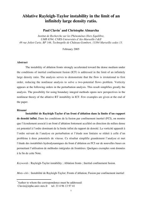
Ablative Rayleigh-Taylor instability in the limit of aninfinitely large density ratio.Paul Clavin * and Christophe AlmarchaInstitut de Recherche sur les Phénomènes Hors Equilibre,UMR 6594, CNRS-Universités d’Aix-Marseille I &II49 rue Joliot Curie, BP 146, Technopôle de Château-Gombert, 13384 Marseille cedex 13.February 2005AbstractThe instability of ablation fronts strongly accelerated toward the dense medium underthe conditions of inertial confinement fusion (ICF) is addressed in the limit of an infinitelylarge density ratio. The analysis serves to demonstrate that the flow is irrotational to firstorder, reducing the nonlinear analysis to solve a two-potential flows problem. Vorticityappears at the following orders in the perturbation analysis. This result simplifies greatly theanalysis. The possibility for using boundary integral methods opens new perspectives in thenonlinear theory of the ablative RT instability in ICF. Few examples are given at the end ofthe paper.RésuméInstabilité de Rayleigh-Taylor d’un front d’ablation dans la limite d’un rapportde densité infini. Dans les conditions de la fusion par confinement inertiel (FCI), on montreque l’écoulement associé à un front d’ablation fortement accéléré en direction du milieu denseest potentiel à l’ordre dominant de la limite infini du rapport de densité. La vorticité apparaît àl’ordre suivant de l’analyse en perturbation et l’étude non linéaire se réduit à celle d’unproblème à deux potentiels de vitesse. Ce résultat simplifie grandement l’analyse et metl’étude des instabilités hydrodynamiques du front d’ablation en FCI sur de nouvelles bases enpermettant l’utilisation de méthodes intégrales de frontières. Quelques exemples sont donnéesà la fin de cette Note.Keywords : Rayleigh-Taylor instability ; Ablation fronts ; Inertial confinement fusion.Mots–clés : Instabilité de Rayleigh-Taylor; Fronts d’ablation; Fusion par confinement inertiel* Author to whom the correspondence must be addressed:Clavin@irphe.univ-mrs.fr tel: 33 4 96 13 97 411

€€€intégrales de frontières que celles utilisées pour l’instabilité de RT avec A =1 [6,7]. Lemodèle de départ a été développé précédemment [2][4], il est constitué d’un front d’ablationd’épaisseur négligeable soumis à un flux thermique fixé à l’infini aval et fortement accéléré€dans la direction de ce flux. La vitesse de propagation du front plan dans le milieu denseest nettement subsonique et l’écoulement au voisinage du front d’ablation est à faible nombrede Mach. Le front est assimilé à une isotherme et les effets hydrodynamiques sont décrits en€supposant la densité constante de part et d’autre du front dans les équations d’Euler,ρ +

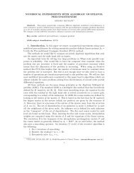
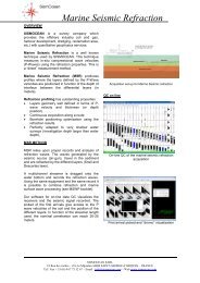
d’Atwood unité [6,7] (Figs 2 & 3). On démontre que, contrairement à la morphologie de lapartie descendante, la vitesse de la bulle n’est pas modifiée par l’ablation. Quelques résultatsnumériques sont présentés, l’étude numérique systématique faisant l’objet d’une autrepublication [8].Fig.1Sketch of temperature and density profiles along the distance x across the unperturbed planarwave.1. IntroductionA major challenge facing inertial confinement fusion is how to control the instabilityof the imploding capsule [1]. Large efforts have been undertaken over the three last decadesto study the ablative Rayleigh-Taylor (RT) instability. The linear theory is now welldeveloped [2], but the non-linear growth of bubbles and spikes is still under investigation[3,4]. As in flame theory, a major difficulty in studying the non-linear growth comes from thevorticity generated in the flow when crossing the ablation front. On the other hand, advanceshave been recently made in the long time evolution of the pure RT instability (inviscid,incompressible fluid without surface tension, bounded by a vacuum), thanks to boundaryintegral methods for potential flow models [6,7]. In this Note, we show that the ablative RTinstability simplifies drastically in the limit of an infinitely large density ratio which is anaccurate approximation in ICF. To first order, the nonlinear analysis reduces to solve twopotential flows. The rotational part of the downstream flow may be taken into account at thesecond order in the perturbation analysis. Numerical results of ablative RT instabilities in ICFmay then be obtained by boundary integral methods. We limit the presentation in this Note tofew examples of periodic solutions in two dimensional geometry compared with the pure RTinstability. Detailed numerical analysis will be published elsewhere [8].4

2. ModelThe model is the same as in references [2] an [4]. The ablation front is an isotherm ofthe downstream flow, θ + (r,t) = θ f >>1 where θ ≡ T /T − is the non dimensional temperaturereduced by its upstream value T − . The temperature is uniform on the cold side θ − =1, and theablation front corresponds to a temperature jump, θ€€f >>1. Density is set constant in the Eulerequations on both sides of the ablation front, ρ€+

layer delimited by the ablation front and the critical surface the equation for the temperatureθ + (r,t) is obtained from the energy conservation,∂(ρ + θ + ) /∂t + ∇.[ρ + u + θ + − ρ − u − l f θ + ν ∇θ + ] = 0. (3)€Eq. (2d) results from a spatial integration of Eq. (3) across the thin ablation front.€€€€€A constant density approximation in Eq. (3) is not compatible with a quasi-isobaricapproximation. The validity of the piecewise constant density model is tricky. The modelconsists in neglecting the flow velocity disturbances induced by the density gradient in the hotregion (downstream the ablation front) in front of those triggered by the deflection of thestream lines across the ablation front. Their ratio is of orderΛ m /d +

of the ablation front controlled by convection-diffusion balance,∂ /∂t >1 ( ρ + /ρ − → 0) and∇.(ρ + u + ) ≈ 0. Notice also that Eq.(4a) is compatible with the steady planar solution of Eq. (3)ρ + u + = ρ − u − i, (θ + −1) − l f θ ν + dθ + /dx = 0, ⇒ d 2 θ ν + /dx 2 ≈ 0€for θ + >>1.€The temperature disturbances generated by the wrinkles of the ablation front die outexponentially quickly over a distance€€ of order Λ toward the hot side. The critical surface is€€not perturbed in the first approximation for Λ >1 and(4c)0 ≤ (x − x f )ν

4. Ordering and scaling laws in the limit ε → 0The linear stability analysis provides us with the ordering in the limitε → 0 [4].Considering 2D perturbations for simplicity, the equation of the perturbed ablation front is€expressed as x = x f (y,t). Using a normal modes decomposition x f € = x ˜ f (k)e ik.y+σt withk ≡ k , any perturbed field can be written asa'(x, y,t) = a ˜ (x,k) x ˜ f (k)e ik.y+σt ,€€€€€µ'= ˜ µ € (k) x ˜ f (k)e ik.y+σt . The solution of the linearized equations € (6a-b) can be expressed interms of three constants of integration˜ U − ,˜ U p+ andU ˜€ r+ as,u ˜ − = U ˜ − e kx ,˜ π − = − σ + k U ˜ − e kx ,(8a)k€ € €u ˜ + = U ˜ p+ e −kx + U ˜ r+ e −εσx , ˜ π + = εσ − k U ˜ p+ e −kx , ik.v ± = −∂u ± /∂x ,(8b)kwhere U ˜ p+ and € U ˜ r+ represent respectively the potential and rotational part of the downstream€flow. The solution of Eqs. (6c) and (7d) yields €€˜€µ (k) = k . where k ≡ k.k . (9a)The constants are obtained from Eqs. (7a-b),˜ U − = k + σ ,(k −εσ) € U ˜ r+ = +2k(σ + k),Finally, by using Eq. (9b) and substituting Eqs. (8a-b) and (9a) forthe following € dispersion relation is obtained,€(1+ ε)σ 2 + 4kσ −[F −1 r (1−ε)k − (1−ε) k 2 ] = 0. €ε(k −εσ) € U ˜ p+ = (1−ε) k 2 − 2kσ − (εσ 2 + k 2 ) . (9b)ε€π ± andµ' into Eq. (7c),(10a)For small ε, the reduced marginal wave number and the reduced maximal growth rate are oforder εF −1€ r and ε 1/ 2 F −1 r respectively. Introducing two quantities of order unity κ and s,€ k ≡ εF −1 r κ , κ = O(1),σ = ε 1/ 2 F −1 r s, s = O(1), (10b)€ the dispersion € relation (10a) takes the simple form s 2 −[κ −κ 2 ] = 0 € at the first € approximationin the limit ε →€€0. The order of magnitude of the€€non dimensional flow fields, expressed interms of the non dimensional amplitude of the perturbed ablation front x f , are obtained from€(8a-b) € and (9a-b),µ =1,µ'/ x f = O(εF r −1 ),u −'u +'/ x f = O(ε 1/ 2 F r −1 ),/ x f = O(F r −1 ),π −'π +'/ x€ f = O(F −1 r ), (11a)/ x f = O(F r −1 ). (11b)€ Notice € that, according to Eqs. € (9b) and (10b), the rotational € part of the downstream flow issmaller than the potential part by a factor ε 1/ 2 . We show in the next section that this is also€€true in the non linear case.€8

5. Nonlinear theory in the limit ε → 0.Considering length and time scales of the same order of magnitude as the mostlinearly amplified wavelength (and its linear growth time), the non dimensional coordinates€useful for solving the non linear problem are, according to Eqs. (5) and (10b),ξ ≡ (εF −1 r )r /l f ,τ ≡ (ε 1/ 2 F −1 r )u − t /l f .(12a)In this system of coordinates,τ andξ = (ξ,η) whereξ andη are the longitudinal and€€€transverse€coordinates, the coordinates€of the ablation front will be denoted by ξ f, solution ofthe unknown equation € of the front €f (ξ f,τ) = 0. € Considering € corrugations of the ablation frontwith amplitude of the same order of magnitude as the most linearly amplified € wavelength, nondimensional quantities of order unity in the limit ε → 0 are introduced from Eqs. (5) (11a-b)€and (12a),m /ρ − u − = µ(ξ f,τ),u n( f ) /u − = ε −1/ 2 U n( f ) ,/u − = ε −1/ €2 'U − (ξ,τ) ,/u − = ε −1 'U + (ξ,τ),The Euler equations (1a) and (6a) yield€⎡ ∂€∂τ + ε1/ 2 ∂ ⎤' ' '⎢ ⎥ U − + (U − .˜ ∇ )U −⎣ ∂ξ⎦u −'u +'€= − ˜ '∇ Π€− ,π −'π +'˜ ∇ .U −'= ε −1 'Π − (ξ,τ),= ε −1 'Π + (ξ,τ),(12b)(12c)= 0 (12d)⎡ε 1/ 2 ∂∂τ + ∂ ⎤' ' '⎢ ⎥ U + + (U + .˜ ∇ )U + = − ˜ '∇ Π + , ˜ '∇ .U + = 0 (12e)⎣ ∂ξ⎦€€where ∇ ˜ denotes the spatial derivative with respect to ξ = (ξ,η). Eqs (12d) express that theunperturbed €€flow is negligible upstream and the perturbed flow is quasi-steady downstream inthe first approximation.€According to Eqs. (11a-b), the normal velocity of the perturbed front and theu n( f )perturbations of the upstream flow velocityu −'are larger than the ablation velocityu − by a€€factor ε −1/ 2 , but smaller than the perturbations of the downstream flow € velocityε 1/ 2 , while the perturbation of the downstream € flowFrom now on, we will consider only the leading order term in the limit ε → 0.€According to Eqs. (7a) mass conservation across the ablation front leads to,€€€'n.U − = U f 'n ,n.(i + U + ) =1+ µ ' .ξ =ξ ξ =ξ €(13a)f fu +'u +'by a factor( fis larger than u ) n by € a factor ε −1/ 2 .The first equation is the same kinematics condition as in the RT problem; to first order, theablation velocity is negligible in front of the upstream flow velocity. Together with the secondequation € (7d) (conservation of energy € at the front) the last equation (13a) yields,n.U +'ξ =ξ f= n.˜ ∇ Ψ ' ξ =ξ f.(13b)€9

On the other hand, according to the first equation (7d),t.˜ ∇ Ψ ' ξ =ξ f= −i.t , together with the€second equation (7b),t.U +'ξ =ξ f= −i.t , one gets,t.U +'ξ =ξ f€= t.˜ ∇ Ψ ' . (13c)ξ =ξ fEquations (13b-c) € then show that the downstream flow is potential at the ablation front,'U + = ∇ ˜ Ψ ' .(14a)ξ =ξ ξ =ξ€ffSince, according to the Euler equations (12e) for constant density, vorticity is simplyconvected downstream and cannot be created elsewhere than across the ablation front, Eq.(14a) shows that the downstream € flow is potential,U +'= ˜ ∇ Ψ ' .(14b)The flow is slaved by the thermal problem, in a way similar to the planar wave in the quasiisobaricapproximation. Without perturbations at ξ = −∞, the upstream flow is also potential,€'U − = ∇ ˜ Φ ' .(14c)The Euler equations (12d-e) may then be written in the simple form€∂€∂τ U '− = −∇ ˜ ' '[ Π − + |U − | 2 /2],∇ ˜ ' ∂.U − = 0,∂ξ U '+ = −∇ ˜ ' 'Π + + |U + | 2 /2leading to the following Bernoulli equations,[ ] ,˜ ∇ .U +'= 0,(15a)'Π − = −∂Φ ' /∂τ− € | ∇ ˜ Φ ' | 2 '/2,Π €€+ = −∂Ψ'/∂ξ− | ∇ ˜ Ψ'| 2 /2, (15b)where two functions of time have been omitted and are incorporated in the definition of thepotentials Φ ' and€be written as,€€Ψ ' . According to the Eq. (7c), the leading order of the pressure jump may€' '[ Π − − Π + ] = (1+ µ') 2 −1− (ξ f −ξ f ) . (15c)ξ =ξf€6. Final resultTo first order, the non linear problem reduces to a free boundary problem, f (ξ f,τ) = 0,consisting in solving two potential flows with a boundary condition (15c) at the front written,according to Eqs. (15b) and the second equation (13a), as⎡− ∂Φ'∂τ + ∂Ψ'∂ξ − | ∇ ˜ Φ'| 2+ | ∇ ˜ Ψ'| 2 ⎤⎢⎥⎣2 2 ⎦ξ =ξ f⎡⎤= ⎢ n.(i + ∇ ˜ Ψ')⎣ξ =ξ⎥f ⎦2€−1− (ξ f−ξ f).i, (16a)€10

€€€€€wherei is the unitary vector in the direction of the acceleration (opposite direction to theenergy flux prescribed at downstream infinity). According to Eqs. (7) and (15a) the twovelocity potentials are solutions of˜ Δ Ψ'= 0˜ Δ Φ'= 0withwithξ → +∞ :ξ → −∞ :Ψ'= 0Φ'= 0,andandΨ' ξ =ξ f= −(ξ f−ξ f).i , (16b)n.˜ ∇ Φ' ξ =ξ f= U n f , (16c)fwhere U n is € the normal € velocity of the front. The last equation (16c) is a purely kinematical€condition in € which the € ablation velocity is negligible in the limit ε → 0.€When the equation of the front may be written in the form ξ = ξ f(η,τ), the reducednormal velocity is defined asn.(i + ˜ ∇ Ψ') ξ =ξ f( fU ) n = (∂ξ f /∂τ)[1+ € (∂ξ f /∂η) 2 ] −1/ 2 , and the relation= [1+ ∂Ψ'/∂ξ ξ =ξ][1+ (∂ξff /∂η) 2 ] 1/ 2 is obtained € by using the second equation(13c). The linear solution is € then recovered from Eq. (16a), by using ∂ξ f /∂τ ≈ ∂Φ'/∂ξ ξ =0andn.(i + € ∇ ˜ Ψ') ≈1+ ∂Ψ'/∂ξ ξ =0 ξ =0.€€€7. Discussion and perspectivesThe only parameter left in Eqs. (16) is the size L of the box, or in non dimensionalform, the inverse of a Froude number, (ρ + /ρ − )gL /2πu 2 − , which measures the number oflinearly unstable modes. We present below numerical € results for two-dimensional periodicsolutions of Eqs. (16) obtained thanks to the boundary integral method used recently for the€Rayleigh-Taylor instability with a unity Atwood number[7]. The results concern two wavenumbers κ = 0,5 (the most linearly amplified one with the reduced growth rate s = 0,5) in fig.2 and κ = 0,1 ( s = 0,3) in fig. 3. We start with a sine-mode whose amplitude equalswavelength/(200π ). The formation of bubbles and spikes is exhibited soon after few€€characteristic linear growth times, typically six. After a time about τ =15 for κ = 0,5 and€ €τ = 30 for κ = 0,1, the bubble velocity reaches the same value as for the classical Rayleigh-€Taylor instability with a unity Atwood number (without ablation). Using a Layzer-type€ €approach [9], it may be easily shown directly from equations (16) that the asymptotic velocity€of the bubble is effectively g/3k . A singularity in the slope appears in the numericalsimulations at τ =12,5 for κ = 0,5 and τ = 21,7 for κ = 0,1. The overall shape looks similar tothe one obtained by Sanz et al. [3]. It is not yet clear that the following orders in the ε€expansion and/or additional curvature terms could regularize the singularity. However, as€ € € €shown in figs. 2 & 3, the numerical simulations have been carried out beyond the occurrence€of the singularity without much trouble by smoothing out the cusp. The tip of the spike is11

strongly affected by ablation. Its acceleration increases and seems to approach g after a timedelay longer than in the Rayleigh-Taylor case. Except in the neighborhood of this tip, theshape of the front is similar to the solution of the classical Rayleigh-Taylor instability with a€unity Atwood number. The relevance of the model and of the numerical results for such largeamplitude of the spike as in figs. 2 & 3 is questionable. Further studies are underinvestigations to clarify the situation [8].It is worth recalling that in real experiments in ICF the duration of implosion istypically 10 times the characteristic growth time of the most amplified wavelength. Thiscorresponds here to τ ≈ 20. Concerning real experiments, reliable predictions require furtherinvestigations. There are two competitive geometrical effects that are not included in thepresent analysis; ablation consumes the spike while implosion amplifies the disturbances€(Bell-Plesset effect). The first one may be taken into account by pushing the analysis to thefollowing order, and the second one is not difficult to be included provided that thewavelength remains small compare to the radius, which is effectively the case. The presentwork will be extended to include these effects in a near future. Another problem to beaddressed with our approach is the wavelength selection when starting with a distributedspectrum of initial disturbances.AcknowledgementsWe wish to thank Laurent Duchemin and Christophe Josserand for providing us withthe boundary integral method to carrying out the direct numerical simulations. Weacknowledge also the support of CEA through grant CEA/DIF 4600051147/P6H29References[1] S. Atzeni, J. Meyer-Ter-Vehn, The physics of inertial fusion, Clarendon Press-Oxford,2004.[2] L. Masse, Étude linéaire de l’instabilité du front d’ablation en fusion par confinementinertiel. Thèse de l’Université de Provence 23 novembre 2001.[3] J. Sanz, J. Ramirez, R Ramis, R. Betti and R.P.J. Town, Nonlinear theory of the ablativeRayleigh Taylor instability, Phys. Rev. Lett. 89, N°19 (2002) 195002-4.[4] P. Clavin, L. Masse Instabilities of ablation fronts in inertial confinement fusion: acomparison with flames, Phys. Plasmas, 11, N°2 (2004) 690-705.[5] B. A. Remington, S.W. Haan, S.G. Glendinning, J. D. Kilkenny, D.H. Munro and R.J.Wallace, Large growth Rayleigh-Taylor experiments used shaped laser pulses. Phys. Rev.Lett. 67 (1991) 3259-62.12

[6] P. Clavin and F. Williams, Asymptotic spike evolution in Rayleigh-Taylor instability, J.Fluid. Mech. 525, (2005) 105-113.[7] L. Duchemin, C. Josserand and P. Clavin, Asymptotic behaviour of the Rayleigh-Taylorinstability, submitted to Phys. Rev. Lett. (2005).[8] C. Almarcha, L. Duchemin, C. Josserand and P. Clavin, in preparation (2005)[9] D. Layzer, On the instability of superposed fluids in a gravitational field. Astrophys. J.122, (1955) 1-12 (1955)FiguresFig.2Two-dimensional solutions of equations (16) at various times. The initial condition isΦ ' (ξ,η,τ = 0) = 0 and a sine-mode for ξ(η,τ = 0) corresponding to the most linearly instable€€wave number k = 0,5εg/u 2 − ( κ = 0,5) with amplitude 0,01/k. At time t =12,5ε −1/ 2 u − /g( τ =12,5), a singularity of the slope appears at the inflexion point on the side of the spike.€€€€€13

Fig.3Two-dimensional solutions of equations (16) at various times. The initial condition isΦ ' (ξ,η,τ = 0) = 0 and a sine-mode for ξ(η,τ = 0) corresponding to the wave number€€k = 0,1εg/u 2 − ( κ = 0,1) with amplitude 0,01/k. At time t = 21,5ε −1/ 2 u − /g − ( τ = 21,5), asingularity of the slope appears€at the inflexion point on the side of the spike.€€€€Figure legendsFig.1Sketch of temperature and density profiles along the distance x across the unperturbed planarwave.14

Fig.1Profils de température et de densité au sein de l’onde plane non perturbée.Fig.2Two-dimensional solutions of equations (16) at various times. The initial condition isΦ ' (ξ,η,τ = 0) = 0 and a sine-mode for ξ(η,τ = 0) corresponding to the most linearly instable€€wave number k = 0,5εg/u 2 − ( κ = 0,5) with amplitude 0,01/k. At time t =12,5ε −1/ 2 u − /g( τ =12,5), a singularity of the slope appears at the inflexion point on the side of the spike.€€€€€Fig.2Évolution de la surface d’ablation au cours du temps à partir d’une perturbation initialesinusoïdale dont la longueur d’onde est linéairement la plus instable k = 0,5εg/u 2 − ( κ = 0,5)et dont l’amplitude vaut 0,01/k. On observe une singularité de pente qui se développe aupoint d’inflexion sur le côté de l’aiguille au temps t =12,5ε −1/ 2 u€ − /g ( τ =12,5).€€Fig.3€€Two-dimensional solutions of equations (16) ) at various times. The initial condition isΦ ' (ξ,η,τ = 0) = 0 and a sine-mode for ξ(η,τ = 0) corresponding to the wave number€€k = 0,1εg/u 2 − ( κ = 0,1) with amplitude 0,01/k. At time t = 21,5ε −1/ 2 u − /g − ( τ = 21,5), asingularity of the slope appears€at the inflexion point on the side of the spike.€€€€Fig.3Évolution de la surface d’ablation au cours du temps à partir d’une perturbation initialesinusoïdale dont la longueur d’onde est k = 0,1εg/u 2 − ( κ = 0,1) et dont l’amplitude vaut0,01/k. On observe une singularité de pente qui se développe au point d’inflexion sur le côté€de l’aiguille au temps€t = 21,5ε −1/ 2 u€ − /g − ( τ€= 21,5).€15