Standard Anatomical and Visual Space for the Mouse Retina ...

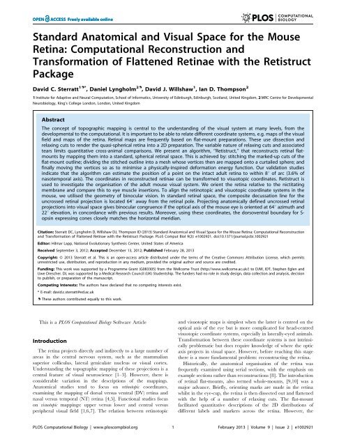
Standard Anatomical and Visual Space for the MouseRetina: Computational Reconstruction andTransformation of Flattened Retinae with the RetistructPackageDavid C. Sterratt 1.* , Daniel Lyngholm 2. , David J. Willshaw 1 , Ian D. Thompson 21 Institute for Adaptive and Neural Computation, School of Informatics, University of Edinburgh, Edinburgh, Scotland, United Kingdom, 2 MRC Centre for DevelopmentalNeurobiology, King’s College London, London, United KingdomAbstractThe concept of topographic mapping is central to the understanding of the visual system at many levels, from thedevelopmental to the computational. It is important to be able to relate different coordinate systems, e.g. maps of the visualfield and maps of the retina. Retinal maps are frequently based on flat-mount preparations. These use dissection andrelaxing cuts to render the quasi-spherical retina into a 2D preparation. The variable nature of relaxing cuts and associatedtears limits quantitative cross-animal comparisons. We present an algorithm, ‘‘Retistruct,’’ that reconstructs retinal flatmountsby mapping them into a standard, spherical retinal space. This is achieved by: stitching the marked-up cuts of theflat-mount outline; dividing the stitched outline into a mesh whose vertices then are mapped onto a curtailed sphere; andfinally moving the vertices so as to minimise a physically-inspired deformation energy function. Our validation studiesindicate that the algorithm can estimate the position of a point on the intact adult retina to within 8u of arc (3.6% ofnasotemporal axis). The coordinates in reconstructed retinae can be transformed to visuotopic coordinates. Retistruct isused to investigate the organisation of the adult mouse visual system. We orient the retina relative to the nictitatingmembrane and compare this to eye muscle insertions. To align the retinotopic and visuotopic coordinate systems in themouse, we utilised the geometry of binocular vision. In standard retinal space, the composite decussation line for theuncrossed retinal projection is located 64u away from the retinal pole. Projecting anatomically defined uncrossed retinalprojections into visual space gives binocular congruence if the optical axis of the mouse eye is oriented at 64u azimuth and22u elevation, in concordance with previous results. Moreover, using these coordinates, the dorsoventral boundary for S-opsin expressing cones closely matches the horizontal meridian.Citation: Sterratt DC, Lyngholm D, Willshaw DJ, Thompson ID (2013) Standard Anatomical and Visual Space for the Mouse Retina: Computational Reconstructionand Transformation of Flattened Retinae with the Retistruct Package. PLoS Comput Biol 9(2): e1002921. doi:10.1371/journal.pcbi.1002921Editor: Hilmar Lapp, National Evolutionary Synthesis Center, United States of AmericaReceived September 3, 2012; Accepted December 13, 2012; Published February 28, 2013Copyright: ß 2013 Sterratt et al. This is an open-access article distributed under the terms of the Creative Commons Attribution License, which permitsunrestricted use, distribution, and reproduction in any medium, provided the original author and source are credited.Funding: This work was supported by a Programme Grant (G083305) from the Wellcome Trust (http://www.wellcome.ac.uk/) to DJW, IDT, Stephen Eglen andUwe Drescher. DL was supported by a Medical Research Council (UK) Studentship. The funders had no role in study design, data collection and analysis, decisionto publish, or preparation of the manuscript.Competing Interests: The authors have declared that no competing interests exist.* E-mail: david.c.sterratt@ed.ac.uk. These authors contributed equally to this work.This is a PLOS Computational Biology Software ArticleIntroductionThe retina projects directly and indirectly to a large number ofareas in the central nervous system, such as the mammaliansuperior colliculus, lateral geniculate nucleus or visual cortex.Understanding the topographic mapping of these projections is acentral feature of visual neuroscience [1–3]. However, there isconsiderable variation in the descriptions of the mappings.Anatomical studies tend to focus on retinotopic coordinates,examining the mapping of dorsal versus ventral (DV) retina andnasal versus temporal (NT) retina [4,5]. Functional studies focuson visuotopic mappings: upper versus lower and central versusperipheral visual field [1,6,7]. The relation between retinotopicand visuotopic maps is simplest when the latter is centred on theoptical axis of the eye but is more complicated for head-centredvisuotopic coordinate systems, especially in laterally-eyed animals.Transformation between these coordinate systems is not intrinsicallyproblematic but does require knowledge of where the opticaxis projects in visual space. However, before reaching this stagethere is a more fundamental problem: reconstructing the retina.Historically, the anatomical organisation of the retina wasfrequently examined using serial sections, with the emphasis onexample sections rather than reconstructions [8]. The introductionof retinal flat-mounts, also termed whole-mounts, [9,10] was amajor advance. Briefly, orienting marks are made in the retinawhilst in the eye-cup, the retina is then dissected out and flattenedwith the help of a number of relaxing cuts. The flat-mountfacilitated quantitative descriptions of the 2D distributions ofdifferent labels and markers across the retina. However, thePLOS Computational Biology | www.ploscompbiol.org 1 February 2013 | Volume 9 | Issue 2 | e1002921

Retistruct: Reconstruction of Flat-mount Retinaerelaxing cuts, together with tears that can occur during flattening,disturbs the retinal geometry significantly, which not onlycomplicates comparison across retinae, but also can be problematicin interpreting results obtained from individual flat-mountedretinae. For example, various measures are used to quantify theregularity of mosaics of various cell types seen in flat-mountedretinae [11,12], but these are susceptible to the existence ofboundaries [13], both at the rim of the retina and those introducedby the relaxing cuts. In the study of topographic mapping, thelocations of ganglion cells labelled by retrograde tracers injectedinto different locations in the target, the superior colliculus, havebeen compared in retinal flat-mounts [4,5]. Foci of labelled cellscan be separated, or even split, by relaxing cuts (see Figure 1A),complicating quantitative analyses.We describe a method to infer where points on a flat-mountretina would lie in a standard, intact retinal space. The standardretina is approximated as a partial sphere, with positions identifiedusing spherical coordinates. Our results show that the method canestimate the location of a point on a flat-mounted retina to within8u of arc of its original location, or 3.6% of the NT or DV axis.This has allowed us to define a standard retinal space for the adultand for the developing mouse eye. Establishing the orientation ofretinal space for the mouse, whose retina contains no intrinsicmarkers, requires experimental intervention. In the Results, wefocus on data from adult mice. We show that a mark based on thecentre of the nictitating membrane is reliable and this mark can berelated to the insertion of the rectus eye muscles. Furthermore, wetransform standard retinal space into visuotopic space and use thegeometry of binocular vision, together with anatomical tracing, toaddress questions about the projection of the optical axis of themouse eye into visual space [3,14,15].Our Retistruct algorithm not only facilitates comparison ofdifferential retinal distributions across animals but also allowsanalyses of distributions of labelled cells in spherical coordinates,obviating the distortions associated with 2D flat-mounts. Finally,transforming retinal coordinates into visual coordinates givesinsights into the functional significance of retinal distributions.Design and ImplementationThe reconstruction algorithmIn this section we give an overview of the reconstructionalgorithm; a more detailed description is contained in theSupplemental Materials and Methods (Text S1). The startingpoint of the algorithm is the flattened retinal outline (Figure 1A),which can include an image or labelled features. In Figure 1A theoutline includes a landmark (blue line), in this case the optic disc,and the locations of retinal ganglion cells that have beenretrogradely labelled following discrete injections of red and greenfluorescent tracers into a retino-recipient central nucleus (thesuperior colliculus). One of the relaxing cuts has bisected thelabelled foci – principally the red one. The first step is to mark thenasal retinal pole (in Figure 1B, ‘‘N’’), which is defined by theperimeter of the long cut towards the optic disc from theperipheral fiducial mark based on the nictitating membrane (seeMaterials and Methods). The locations and extents of cuts andtears in the outline are also marked up (cuts 1–4 in Figure 1B).Because the retina in the eye-cup is more than hemispherical, theangle of the retinal margin (rim angle) measured from the pole ofthe retina is then supplied (Table 1 and see later section below).The outline is then divided into a mesh containing at least 500triangles of roughly equal size, and the cuts and tears are stitchedtogether (Figure 1C). This mesh is then projected onto a sphericalsurface, with all the points on the retinal margin lying on the circledefined by the rim angle (Figure 1Di). Each edge in the mesh istreated as a spring whose natural length is the length of thecorresponding edge in the flat mesh. It is not possible to make thisinitial mapping onto the spherical surface optimal, so the springsare either compressed (blue), expanded (red) or retain their naturallength (green). In the next step the springs are allowed to relax soas to minimise the total potential energy contained in all thesprings, leading to the refined spherical mesh shown in Figure 1Ei.The locations of mesh points in the flat-mount and theircorresponding locations on the sphere define the relation betweenany point in the flat-mount and a standard spherical space. Thisrelation is used to map the locations of data points and landmarksin the flat retina onto the standard retina. These can be visualisedinteractively on a 3D rendering of a sphere (see Figure 1D), orrepresented using a map projection such as the azimuthalequidistant projection centred on the retinal pole (Figure 1Fi). Inall plots of retinal space we use the colatitude and longitudecoordinate system, where colatitude is like latitude measured onthe globe, except that zero is the pole rather than the equator.Map projections [16] such as that in Figure 1Fi are very useful forrendering retinal label into a standard retinal space. An alternativerepresentation is shown in Figure 1Dii,Eii,Fii, where lines oflatitude and longitude on the standard spherical retina have beenprojected onto the flat structure. The jump between Figure 1Diiand 1Eii illustrates the improvement in the appearance of themapping achieved after minimising the energy.In order to analyse data points on the standard retina, we usedspherical statistics [17]. The mean locations of groups of datapoints on the sphere (diamonds in Figure 1Fi) are computed usingthe Karcher mean and we used density estimation to producecontour plots (see Supplemental Materials and Methods, Text S1).Performance of the algorithmTo assess the amount of residual deformation at the end of theenergy minimisation procedure, we plotted the length of each edgei in the spherical mesh l i versus the length of the correspondingedge in the flat mesh L i (Figure 2A), using the same colour scale asin Figure 1D,E. A measure of the overall deformation ofreconstruction is:vffiffiffiffiffiffiffiffiffiffiffiffiffiffiffiffiffiffiffiffiffiffiffiffiffiffiffiffiffiffiffiffiffiffiffiffiu 1 X (l i {L i ) 2e L ~ t2DCDLwhere the summation is over C, the set of edges, the mean lengthof an edge in the flat mesh is L, and the number of edges is DCD.Physically, this measure is the square root of the elastic energycontained in the notional springs. It is constructed so as to be of asimilar order to the mean fractional deformation.We used our algorithm on 297 flat-mounted retinae, 288 ofwhich could be reconstructed successfully, 7 of which failed due to,as-yet unresolved, software problems and 2 of which were rejectedbecause of unsatisfactory reconstructions (see below). Figure 2Ashows the reconstruction with the lowest deformation measuree L ~0:038 and Figure 2E the example with a high value ofe L ~0:118. The arrangement of the grid lines in the example withlower deformation looks qualitatively smoother and more eventhan in the example with higher deformation measure(Figure 2C,G). The strain plot for the retina with the lowerdeformation (Figure 2B) indicates that almost all edges areunstressed, whereas in the retina with higher deformation(Figure 2F) there are many more compressed and expandededges. It can be seen that the retina in Figure 2E–H has a muchi[CL ið1ÞPLOS Computational Biology | www.ploscompbiol.org 2 February 2013 | Volume 9 | Issue 2 | e1002921

Retistruct: Reconstruction of Flat-mount RetinaeFigure 1. Overview of the method. A, The raw data: a retinal outline from an adult mouse (black), two types of data points (red and green circles)from paired injections into the superior colliculus and a landmark (blue line). B, Retinal outline with nasal pole (N) and cuts marked up. Each pair ofdark cyan lines connects the vertices and apex of the four cuts. C, The outline after triangulation (shown by grey lines) and stitching, indicated bycyan lines between corresponding points on the cuts. Di, The initial projection of the triangulated and stitched outline onto a curtailed sphere. Thestrain of each edge is represented on a colour scale with blue indicating compression and red expansion. Cuts are shown in cyan. Dii, The strainplotted on the flat outline with lines of latitude and longitude superposed. Ei,ii, As Di,ii but after optimisation of the mapping. Fi, The datarepresented on a polar plot of the reconstructed retina. Mean locations of the different types of data points are indicated by diamonds. The nasal (N),dorsal (D), temporal (T) and ventral (V) poles are indicated. Cuts are shown in cyan. Fii, Data plotted on the flat representation, with lines of latitudeand longitude superposed. All scale bars are 1 mm.doi:10.1371/journal.pcbi.1002921.g001less distinct margin than in Figure 2A–D. This makes it harder forthe algorithm to create an even mapping, as local roughness in therim forces significant deformation of the surrounding virtual tissuewhen morphed onto the sphere.Thus the deformation measure e L gives some indication of theapparent quality of the reconstruction. A value greater than 0.2indicates a problem with the stitching part of the algorithm; the 2such reconstructions were rejected and are not included in the 288PLOS Computational Biology | www.ploscompbiol.org 3 February 2013 | Volume 9 | Issue 2 | e1002921

Retistruct: Reconstruction of Flat-mount RetinaeTable 1. Measurements of mouse eyes at various stages ofdevelopment.Age d e (mm) d r (mm) Q 0 (6)P0 1632617 1308617 127.1361.92P2 2146613 1780629 131.2062.20P4 225069 1857620 130.5861.40P6 2450641 1963625 127.0262.41P8 264661 2088634 125.3161.81P12 2786615 2212665 126.0363.37P16 2808617 2043617 117.1060.96P22 2958635 2117644 115.5762.17P64 3160656 2161630 111.5661.89The distance from the back of the eye to the surface of the cornea d e ,theperpendicular distance from the back of the eye to the rim of the retina d r andthe rim colatitude Q 0 derived from this. Each measurement is averaged over theright and left eyes of two different animals, i.e. over four eyes in total.doi:10.1371/journal.pcbi.1002921.t001successful reconstructions. Noticeably bad reconstructions tend tohave e L w0:1. We recommend checking the mark-up of cuts andtears in any retinae with e L w0:1. The mean deformation measurewas 0.071, the median was 0.070 (Figure 3A), and 27 out of 288retinae had a deformation measure exceeding 0.1, including theretina illustrated in Figure 2E–H as an, intentionally, poordissection. With e L = 0.118, it falls above the 97.5th percentile ofthe retinae illustrated in Figure 3A. The larger deformations tendto come from younger animals (Figure 3B), reflecting the difficultyof dissecting retinae out of these animals cleanly due to the moredelicate nature of younger tissue.It should be noted that retinae which have lost tissue due topoor dissection can be forced onto the spherical surface by thealgorithm, albeit with high e L values. Reconstruction of suchretinae should not be attempted, since remaining tissue will bemapped to inappropriate regions of the sphere.Determination of the rim angleTo determine the rim angle of mouse eyes at varying stages ofdevelopment we measured the distance d e from the back of the eyeto the front of the cornea and the distance d r from the back of theeye to the edge of the retina (Figure 3C). We then computed thecolatitude (the angle measured from the retinal pole) Q 0 of the rimusing the formula:Q 0 ~arccos(1{2d r =d e )The measurements and derived latitudes for animals of variousages are shown in Table 1.An alternative approach to setting the rim angle is to infer, foreach individual retina, the rim angle that minimises thedeformation. This was done by repeating the minimisation forrim angles at 1u intervals within a range ½{20 0 ,z5 0 Š of the rimangle determined by measurement as above. A comparison of themeasured and inferred rim angles is shown in Figure 3D. It can beseen that inferred rim angle is usually less than that obtained frommeasurements of standard retinae. Figure 3E shows a comparisonof the reconstruction error obtained using the measured andinferred rim angles. The maximum decrease in the reconstructionerror is 19.1%, with the mean improvement being 7.2%. Weð2ÞFigure 2. Examples of reconstructed retinae. A–D, An example of a reconstruction of an adult retina with low deformation measure e L ~0:038.A, Plot of length of edge on the sphere versus length of edge on the flat retina. Red indicates an edge that has expanded and blue a edge that hasbeen compressed. B, The log strain ln l i =L i indicated using the same colour scheme on the flat retina. C, The flat representation of lines of latitudeand longitude with the optic disc (blue). D, The azimuthal equidistant (polar) representation showing the locations of the cuts and tears (cyan) andthe location of the optic disc (blue). E–H, An example of a reconstruction of a P0 retina with high deformation energy e L ~0:118. Meaning of E–Hsame as for corresponding panel in A–D. All scale bars are 1 mm.doi:10.1371/journal.pcbi.1002921.g002PLOS Computational Biology | www.ploscompbiol.org 4 February 2013 | Volume 9 | Issue 2 | e1002921

Retistruct: Reconstruction of Flat-mount Retinaedisc location (Figure 4C). If reconstructions require accuracy toless than 7.4u, this could be achieved by increasing the stringencyof e L values used to reject reconstructions. Rounding up this errorgives a value of 8u, which is 3.6% of the 223u along thenasotemporal axis of the adult eye. It is worth noting that the errorof reconstruction depends not only on the algorithm, but also thedata presented to it, which is intrinsically variable.ResultsFigure 3. Deformation of reconstructions and the effect of rimangle. A, Histogram of the reconstruction error measure e L obtainedfrom 288 successfully reconstructed retinae. B, Relationship betweendeformation measure and age. ‘‘A’’ indicates adult animals. C,Schematic diagram of eye, indicating the measurements d e and d rmade on mouse eyes at different stages of development, and the rimangle Q 0 derived from these measurements. Note that rim angle ismeasured from the optic pole (*). D, Rim colatitude ^Q 0 that minimisesreconstruction error versus the rim angle Q 0 determined from eyemeasurements. Solid line shows equality and grey lines indicate 610uand 620u from equality. E, Minimum reconstruction error e L obtainedby optimising rim angle versus reconstruction error e L obtained whenusing the rim angle from eye measurements. Solid line indicatesequality.doi:10.1371/journal.pcbi.1002921.g003concluded that this improvement was not sufficiently great to addautomatic refinement of the rim angle to the algorithm.Estimate of errors of the reconstruction algorithm fromoptic disc locationThe deformation measure gives an indication of how easy it is tomorph any particular flattened retina onto a partial sphere, but itdoes not indicate the error involved in the reconstruction, i.e. thedifference between the inferred position on the spherical retinaand the original position on the spherical retina. The ideal methodfor estimating the error would be to flatten a retina marked inknown locations, and then compare the inferred with the knownlocations. However, this proved to be technically very difficult andso we tried another method of estimating the error that uses theinferred locations of the optic discs across a number of retinae. Inmice, the optic disc is located ‘‘rather precisely in the geometriccenter of the retina’’ [18], though this has not, as far as we areaware, been measured. We marked the optic disc in 72 flatmountedadult retinae, and the distribution of the centres of theinferred locations of these optic discs is shown in Figure 4A,B. Themean colatitude and longitude of these optic discs is (3.7u, 95.4u)with a standard deviation of 7.4u. The mean is therefore 3.7u awayfrom the geometrical centre of the retina, in good agreement withthe qualitative observation that the optic disc is at the geometriccentre of the retina. Under the, questionable, assumption thatnone of the variability is biological, this suggests that an upperbound on the accuracy of the reconstruction algorithm is 7.4u.There is a significant relationship between the deformation errore L and the inferred distance of the optic disc from the mean opticDistributions of ipsilateral and contralateral retinalprojectionsWe now describe the first application of the reconstructionalgorithm. The relationship between the projections from themouse retina to the ipsilateral and contralateral dLGN has beenstudied in retina flat-mounts following injection of retrogradetracer into the dLGN [3]. Reconstructing the retinae of individualanimals that have had retrograde tracer injected into primaryvisual areas enables comparisons of projection patterns acrossanimals independent of distortions introduced by retinal dissection.Moreover, having a standard retinal space means that datafrom multiple animals can be used to create aggregate topographicmaps.The reconstruction method has enabled the quantification ofthe binocular projection from the retina to the dLGN acrossmultiple animals. To label the projection, the dLGN in adult micewas injected either with Fluoro-Ruby or Fluoro-Emerald. Further,in some animals, the injections were bilateral (see Figure 5A andSupplemental Materials and Methods, Text S1, for details). TheRetistruct program was used to reconstruct the retinae. The plotsin Figures 5B–D show the label in one retina from an animal thathad received bilateral injections into the dLGN (Figure 5A). Theseplots were done using an in-house camera-lucida set-up, samplingthe entire ventrotemporal crescent for the ipsilateral retina andone in nine 150 m square boxes for the contralateral label(Figure 5B). The ipsilateral projection (Figure 5C) is restricted tothe ventrotemporal crescent whereas label from the contralateralprojection (Figure 5D) is distributed widely. The nature of theoverlap between the uncrossed and crossed projections is evidentin Figure 5B. Having reconstructed the retinae into a standardspace, we quantified the projection patterns by deriving kerneldensity estimates (KDEs) of the underlying probability of datapoints appearing at any point in the retina and represented theseestimates using contours that exclude 5%, 25%, 50% and 95% ofthe points (Figure 5C). In the case of the contralateral label, theFigure 4. Estimation of reconstruction error using optic disclocation. A, Inferred positions of optic discs from 72 adultreconstructed retinae plotted on the same polar projection. Thecolatitude and longitude of the Karcher mean is (3.7u, 95.4u). Thestandard deviation in the angular displacement from the mean is 7.4u.B, The same data plotted on a larger scale. C, The relationship betweenthe deformation of the reconstruction and distance e OD of the inferredoptic disc from the population mean. There was a significant correlationbetween the two (R 2 ~0:35,pv0:01).doi:10.1371/journal.pcbi.1002921.g004PLOS Computational Biology | www.ploscompbiol.org 5 February 2013 | Volume 9 | Issue 2 | e1002921

Retistruct: Reconstruction of Flat-mount Retinaedata consisted of cell counts within defined boxes on the flattenedretina. Here we used kernel regression (KR) as the source for thecontouring algorithm (Figure 5D; see Supplemental Materials andMethods, Text S1, for details). The Karcher mean of the datapoints is represented by the magenta and cyan diamonds in eitherplot and the peak density for the kernel is represented by the bluediamond. It is worth noting that these two measures often givedifferent locations, as would be expected from skewed distributions.Obtaining uniform and complete injections of tracer into thedLGN can be difficult and can result in variability in the pattern oflabel (e.g. the contralateral retinae in Figure 6A). We have takenadvantage of standard retinal space to measure the extent of theipsilateral projection by making a composite plot of data from 7different animals (Figure 5E), which shows that the averageipsilateral projection occupies a crescent in ventrotemporal retina.The decussation line for the aggregate ipsilateral population is64.161.6u from the retinal pole, which in these 7 animals is veryclose to the optic disc. The distance from the optic disc to thedecussation line is 63.461.3u (Figure 5F). The ipsilateral crescentspans an average of 134.161.5u of the rim extending from22.161.3u beyond the temporal pole to 22.061.5u beyond theventral pole (Figure 5G).Transformation to visuotopic coordinatesThe geometry of binocular vision implies that the ipsilateraldecussation line should correspond to the vertical meridian in theadult mouse’s visual field [3,6]. In order to investigate thisprediction, we sought to map the retina onto visual space. Themapping of visual space onto the retina is determined by theorientation of the optic axis and the optics of the eye. We assumethat the optic axis corresponds to the retinal pole of the sphericalretinal coordinate system. Thus the optic axis is close to but notcoincident with the optic disc. The location of the optic disc hasbeen estimated to be projected to a point 60u lateral to the verticaland 35u above the horizontal meridian in anaesthetised mice [14].Alternatively, the optic axis has been reported to be 64u lateral tothe vertical and 22u above the horizontal meridian in ambulatorymice [15]. In anaesthetised mice, Dräger and Hubel noted that theeyes were always diverted outwards [1].In principle, the deviation of a ray by the eye can be estimatedby means of a schematic model of the mouse eye [19,20]. WeFigure 5. Measurement of the ipsilateral projection. A, Schematic illustrating the retinal label resulting from bilateral injections of Fluoro-Ruby(magenta) and Fluoro-Emerald (cyan) dye into the dLGN. B, Flat-mounted retina with label resulting from bilateral injections of Fluoro-Ruby(magenta) and Fluoro-Emerald (cyan) into left and right dLGN, respectively. C–D, Azimuthal equilateral projection of reconstructed retina in B.Isodensity contours for 5%, 25%, 50%, 75% & 95% are plotted using the kernel density estimates (KDEs) for fully sampled retinae (C) or kernelregression (KR) estimates for partially sampled retinae (D). Blue diamond is the peak density and magenta (C) or cyan (D) diamond is the Karchermean. Yellow circle is the optic disc. E, Composite plot with ipsilateral label from unilateral injections (n~7). Black dashed lines represent the medianangle from the optic axis to the peripheral edges of the 5% isodensity contour. Coloured diamonds represent the Karcher means of the label in theindividual retinae and large coloured circles are the optic discs for the individual retinae. White square and circle represent the average Karcher mean.The central dashed angle represents the median central edge of the 5% isodensity contour. F, Mean distances from either optic disc or optic axis ofreconstructed retinae to the central edge of the 5% isodensity contour along a line passing through the Karcher mean of the label. G, The extent ofthe ipsilateral label and the distance beyond the horizontal and vertical axes. Grid spacing is 20u. In F–G, line represents the mean and error bars arestandard error of the mean. Scale bar in C & D is 1 mm.doi:10.1371/journal.pcbi.1002921.g005PLOS Computational Biology | www.ploscompbiol.org 6 February 2013 | Volume 9 | Issue 2 | e1002921

Retistruct: Reconstruction of Flat-mount RetinaeFigure 6. Alignment of the binocular zone in visuotopic coordinates. A, Azimuthal equilateral projections in standard retinal space of leftand right retinae with ipsilateral (upper) and contralateral (lower) label resulting from bilateral injections of Fluoro-Ruby (magenta) and Fluoro-Emerald (cyan) into left and right dLGN, respectively, of the same mouse. Plots were generated from stitched 106 epifluorescent images and celllocations detected using ImageJ. For this figure, we have abandoned the convention of always plotting nasal retina to the right. B, Schematicillustrating the approximate projection of retinal space onto visual space. When the orientation of the optic axis (grey line) is optimal, the ipsilateralcrescent is projected entirely to the opposite visual field. Note that due to the refraction in the lens the visual field is estimated to be 180u for eacheye. C–D, Orthographic projections in central visuotopic space of the two ipsilateral retinae in A with optic axis (*) at 64u azimuth; 22u elevation (C)and with optic disc at 60u azimuth; 35u elevation (D). E, Sinusoidal projection of contralateral retinae in B with the optic axis (*) at 64u azimuth; 22uelevation. Labels N, D, T, V indicate the projection of the corresponding pole of the retina. Grid spacing is 15u.doi:10.1371/journal.pcbi.1002921.g006investigated using one such model [20] to determine the deviationof paraxial rays. The schematic eye model is not, however,constructed to account for wide-field rays, so we decided toapproximate the effect of the optics of the eye by making thedeviation of a rays passing through the posterior nodal point of theeye, which is approximately the centre of the eye, proportional tothe ray’s angle of incidence. The constant of proportionality issuch that rays at 90 to the eye will be projected onto the edge ofthe retina, regardless of the retina’s rim angle (see Figure 6B). Themapping of the eye onto visual space is effected by a coordinatetransformation in which first the approximate optics are used toproject points on the retina through the centre of the eye onto anotional large concentric sphere about the eye representing visualspace. Then the locations of the points on this ‘‘celestial’’ sphereare measured in terms of elevation, the angle above the horizontaland azimuth, the angle made between the point’s meridian planeand the zero meridian plane, i.e. the vertical plane containing thelong axis of the mouse. By convention [3,6,14], projections ofvisual space are presented as though the mouse is sitting facing theobserver, so that the azimuth angle is positive in the left visualfield.Using the above conventions to test whether the position of theipsilateral decussation line corresponds to the vertical meridian invisuotopic space, we have transformed the retinotopic location ofipsilateral retinal ganglion cells, following bilateral injections, intohead-centred visuotopic space [21]. To minimise between-animalvariability, we used bilateral injections into the dLGN: injectingFluoro-ruby on one side and Fluoro-emerald on the other side (seeFigure 5A). Figure 6A illustrates the distribution of retrogradelylabelledganglion cells in the ipsilateral (upper plots) and contralateral(lower plots) retinae. For this Figure, we have abandoned thestandard representation of the nasal retina to the right in order toemphasise the mirror-symmetry of the projections. Injection ofFluoro-emerald into the right dLGN leads to label restricted to theventrotemporal crescent in the right retina but widespread labellingin the left retina; a complementary pattern is seen for an injection ofFluoro-ruby into the left dLGN. When the retinal distribution of theipsilateral ventrotemporal crescent neurons is transformed intovisuotopic space using the optic axis coordinates of 64u azimuth and22u elevation [15], and plotted in an orthographic projection of thecentral visual field, the decussation line lines up with the verticalmeridian. These plots have been rotated with 50u elevation toinclude the upper part of the visual field beyond 180u (Figure 6C). If,in contrast, the ipsilateral projection is transformed using the opticdisc coordinates of 60u azimuth and 35u elevation [14], there is anevident visual mismatch between the two decussation lines(Figure 6D). To examine the visuotopic extent of the contralateralprojection in the two eyes, we displayed the data in a sinusoidal mapprojection to include the full visual field through both eyes(Figure 6E). This demonstrates that the decussation pattern in thecontralateral projection is not as sharp as that in in the ipsilateralprojection. Intriguingly, it appears that inferior-central field, a regionthat would be shadowed by the nose, is also under-represented.Given these observations and our group data for optic disclocation (Figure 5E), this indicates a revised optic disc projection of66u azimuth and 25u elevation. Having fixed the location of theeye in visual space, our data on the uncrossed projection predictthat the width of binocular visual field is 52u at its greatest width,slightly larger than the 30–40u of Dräger and Hubel [1], but withinthe range of 50–60u estimated by Rice et al. [22] and ColemanPLOS Computational Biology | www.ploscompbiol.org 7 February 2013 | Volume 9 | Issue 2 | e1002921

Retistruct: Reconstruction of Flat-mount Retinaeet al. [3]. The binocular field starts a few degrees below thehorizon and continues well behind the animal’s head – very likethe situation in the rabbit [23].Eye muscles and S-opsin in retinal and visuotopiccoordinatesTo examine the orientation of the eye, the locations of theinsertions of superior, lateral and inferior rectus into the globe ofthe eye were marked onto the retina (Figure 7A; see SupplementalMaterials and Methods, Text S1, for procedure). The nasal pole ofthe retinae is determined with reference to the nictitatingmembrane. The retinae were reconstructed and plotted in anazimuthal equidistant polar projection and the vectors connectingthe insertion points and the optic disc were plotted (Figure 7B).Once in a standard space, the muscle insertion points (n~33) fromall the retinae (n~17) were plotted in the same plot and thevectors connecting the Karcher mean of each muscle insertion andthe Karcher mean for the optic disc location were plotted(Figure 7C). Figure 7D shows the mean vector angles: lateralrectus, at 184.963.6u, is directly opposite the nasal cut, superiorrectus is at 91.365.9u and inferior rectus is at 284.264.1u,wherenasal is 0u. It is noticeable that there is considerable variability inthe locations of the muscle insertions, certainly when compared tothe variability of the optic discs. A considerable contributory factorin this is the large extent of the muscle and the relative difficulty indetermining the centre of the muscle.The location of the optic axis at 64u azimuth and 22u elevation[15] determines the location of the vertical and horizontalmeridians on the eye. The location of the ipsilateral decussationline confirms this azimuthal value (Figures 5E & 6C). As the mouseretina has no pronounced horizontal streak, we looked at thedistribution of short wavelength opsin (S-opsin) in the retina.Haverkamp et al. [24] describe a very distinct distribution patternin the retina, with high density ventral, low density dorsal and anabrupt transition and suggested that the transition coincided withthe horizontal meridian. Figure 8A shows immuno-staining for S-opsin from dorsal, central and ventral retina. The densitydifference between dorsal and ventral is marked and the transitionis abrupt. Figure 8B & 8C illustrate the transformation of the S-opsin distribution from retinal flat-mounts to standard retinalspace to an orthographic representation of visuotopic spacecentred on the optic axis. In these plots, the transition is3.360.3u above the horizontal meridian at the level of the opticaxis and is tilted by 13.863.6u, so that transition is 7.862.0u abovethe horizontal meridian in central visual field and 6.061.6u belowthe horizontal meridian peripherally (Figure 8D). The label fromboth left and right retinae was also plotted in a sinusoidalprojection (Figure 8D) to illustrate that the rotation seen in theorthogonal plots for each eye is symmetric along the verticalmeridian of the entire visual field (Figure 8E).In summary, with the location of the optic axis determined bythe optimal match of the decussation line with the verticalmeridian, the change in S-opsin staining nicely coincides with thehorizontal meridian, at least for the central visual field, aspredicted by Szél et al. [25]. It is worth noting that S-opsin ismostly co-expressed with medium wavelength opsin (M-opsin)[24,26], and that this would make these cones in upper visual fieldrespond to a broader spectrum, which may have implications forthe ability to detect a larger range of objects above the mouse. Theprecise distribution of S-opsin is not uniformly agreed upon [24–26]. However, when plotting the distributions from Szél et al [25]to visuotopic space using Retistruct (data not shown), we get a verysimilar distribution to that seen in Figure 8B–C.Figure 7. Measurement of muscle insertion angles. A, Flatmountedretina showing stitching and insertions for superior rectus(red), lateral rectus (green) and inferior rectus (blue). N indicates nasalcut. Plots on right represent the distortions introduced by reconstructingretina (see Figure 2 for explanation). B, Azimuthal equilateralprojection of reconstructed retina in A. Dashed lines represent vectorsconnecting muscle insertion point to the optic disc. C, Muscle insertionpoints from 17 retinae. Solid black circles represent the optic discs forindividual retinae. Dashed lines represent the line from each individualinsertion point to its respective optic disc. Solid lines are from theKarcher mean insertion to the Karcher mean location of the optic disc.Grid Spacing is 15u. D, Plot of the angles of the angles of vectorsconnecting muscle insertions of Superior Rectus (SR), Lateral Rectus (LR)and Inferior Rectus (IR) to the individual optic discs. Bar represents themean and error-bars are standard deviation.doi:10.1371/journal.pcbi.1002921.g007Availability and Future DirectionsThe reconstruction and transformation methods described herehave been implemented in R [27] and use the Triangle library[28] for mesh generation. The retinae in this paper werereconstructed and analysed using version 0.5.7 of the Retistructpackage (Dataset S1). The package, including full installationinstructions, is also available anonymously and for free under theGPL license from http://retistruct.r-forge.r-project.org/. Thepackage has been tested with R version 2.15.2 on GNU/Linux(Ubuntu 12.04), MacOS X 10.8 and Microsoft Windows Vista.The user guide, available from the same site, contains details of thetwo main data formats Retistruct can process. These are either inthe form of coordinates of data points and retinal outline from anin-house camera-lucida setup, or in the form of bitmap imageswith an outline marked up in ImageJ ROI format [29]. There is aGUI interface to facilitate the marking-up of retinae anddisplaying reconstructed retinae.The program could be applied to flat-mount preparations ofretinae from any vertebrate species at any age, provided the globeof the eye is approximately spherical, and it would be possible toadd extra analysis routines. When examining retinae with mosaiclabelling [30], reconstructing the retina into its original sphericalcoordinates would make it possible to determine more accuratelythe relative distances between cells between peripheral and centralretina. To implement mosaic analysis would require computationof a Voronoi tessellation on the sphere, which could beimplemented by doing the Voronoi tessellation on a conformal(Wulff) projection [31]. Further visualisation methods could alsoPLOS Computational Biology | www.ploscompbiol.org 8 February 2013 | Volume 9 | Issue 2 | e1002921

Retistruct: Reconstruction of Flat-mount RetinaeFigure 8. Visuotopic axes with respect to S-opsin distribution. A, S-opsin staining in dorsal, central and ventral retina. Images acquired at206magnification. Scale bar is 100 m. B–C, S-opsin distribution for right (A) and left (B) eyes plotted in orthographic projection centred on optic axis(*) at 22u elevation and 64u azimuth. Bottom left plot is flat-mounted retina. Bottom right plot is azimuthal equilateral plot. Plots were generated fromstitched 106 epifluorescent images and cell locations detected using ImageJ [29]. There are slight differences between the two eyes in the exactangle of density transition with respect to the horizontal meridian and in the density of staining around the optic disc. These will reflect experimentalvariance. Again our normal convention of showing nasal to the left has been relaxed. Scale bar is 1 mm. D, The average offset of the S-opsin densitytransitionfrom the horizontal meridian in central and peripheral visual field (n~9). Error bars are SEM. E, S-opsin distribution for both eyes plotted ina sinusoidal projection with same optic axis (*) as in C. Yellow outline is edge of left retina; red outline is edge of right retina. Labels N, D, T, V indicatethe projection of the corresponding pole of the retina. Grid spacing is 15u.doi:10.1371/journal.pcbi.1002921.g008be added. Using equations similar to those in the literature [21],locations on the retina could be projected onto a screen placedorthogonal to the optic axis, thus enabling a direct translation ofvisual stimulus space onto retinal coordinates. It would also bepossible to map visual space onto retinal coordinates, by invertingthe operations to map the retina onto visual space.It should be stressed that the current version is not intended foruse on partial retinae. However, it might eventually be possible tolocate incomplete retinae in standard retinal space, if there enoughmarkers to orient the partial retina correctly. Similarly, it shouldbe possible to locate sections (either histological or tomological) ofknown orientation and hemiretinal origin in standard space.Supporting InformationDataset S1 Complete source code for the Retistruct package(version 0.5.7). Includes demonstration data for Figures 1, 2 and 6in this paper, a user guide with installation instructions, and areference manual containing descriptions of the functions used inthe package.(ZIP)References1. Dräger UC, Hubel DH (1976) Topography of visual and somatosensoryprojections to mouse superior colliculus. J Neurophysiol 39: 91–101.2. McLaughlin T, O’Leary DD (2005) Molecular gradients and development ofretinotopic maps. Annu Rev Neurosci 28: 327–355.3. Coleman JE, Law K, Bear MF (2009) Anatomical origins of ocular dominance inmouse primary visual cortex. Neuroscience 161: 561–571.Text S1 Supplemental information including an extendedDiscussion, and Materials and Methods containing details ofexperiments and detailed description of the reconstructionalgorithm and analysis of reconstructed data.(PDF)AcknowledgmentsThe authors would like to thank Andrew Lowe, Stephen Eglen, Johannes J.J. Hjorth, and Michael Herrmann for their very helpful commentsthroughout this work. We would also like to thank Nicholas Sarbicki forhelping with the analysis of LGN projections and Henry Eynon-Lewis forassistance with dissections for muscle-insertion marking and S-opsinstaining. We thank anonymous reviewers for alerting us to futurepossibilities of using Retistruct to map partial or sectioned retinae ontostandard retinal space.Author ContributionsConceived and designed the experiments: DCS DL IDT. Performed theexperiments: DL IDT. Analyzed the data: DCS DL IDT. Contributedreagents/materials/analysis tools: DCS. Wrote the paper: DCS DL DJWIDT. Wrote the software package: DCS.4. Reber M, Burrola P, Lemke G (2004) A relative signalling model for theformation of a topographic neural map. Nature 431: 847–853.5. Rashid T, Upton AL, Blentic A, Ciossek T, Knöll B, et al. (2005) Opposinggradients of ephrin-As and EphA7 in the superior colliculus are essentialfor topographic mapping in the mammalian visual system. Neuron 47: 57–69.PLOS Computational Biology | www.ploscompbiol.org 9 February 2013 | Volume 9 | Issue 2 | e1002921

Retistruct: Reconstruction of Flat-mount Retinae6. Dräger UC, Olsen JF (1980) Origins of crossed and uncrossed retinal projectionsin pigmented and albino mice. J Comp Neurol 191: 383–412.7. Haustead DJ, Lukehurst SS, Clutton GT, Bartlett CA, Dunlop SA, et al. (2008)Functional topography and integration of the contralateral and ipsilateralretinocollicular projections of ephrin-A 2/2 mice. J Neurosci 28: 7376–7386.8. Lashley KS (1932) The mechanism of vision. V. The structure and imageformingpower of the rat’s eye. J Comp Psychol 13: 173–200.9. Stone J (1981) The Whole Mount Handbook: A Guide to the Preparation andanalysis of retinal whole mounts. Sydney: Maitland Publications. 128 p.10. Ullmann JFP, Moore BA, Temple SE, Fernández-Juricic E, Collin SP (2012)The retinal wholemount technique: A window to understanding the brain andbehaviour. Brain Behav Evol 79: 26–44.11. Wässle H, Boycott BB (1991) Functional architecture of the mammalian retina.Physiol Rev 71: 447–480.12. Raven MA, Eglen SJ, Ohab JJ, Reese BE (2003) Determinants of the exclusionzone in dopaminergic amacrine cell mosaics. J Comp Neurol 461: 123–136.13. Cook JE (1996) Spatial properties of retinal mosaics: An empirical evaluation ofsome existing measures. Visual Neurosci 13: 15–30.14. Dräger UC (1978) Observations on monocular deprivation in mice.J Neurophysiol 41: 28–42.15. Oommen BS, Stahl JS (2008) Eye orientation during static tilts and its relationshipto spontaneous head pitch in the laboratory mouse. Brain Res 1193: 57–66.16. US Geological Survey. Map projections. Available: http://egsc.usgs.gov/isb/pubs/MapProjections/projections.html. Accessed 5 July 2012.17. Fisher NI, Lewis T, Embleton BJJ (1987) Statistical analysis of spherical data.Cambridge, UK: Cambridge University Press. 344 p.18. Dräger UC, Olsen JF (1981) Ganglion cell distribution in the retina of themouse. Invest Ophth Vis Sci 20: 285–93.19. Remtulla S, Hallett PE (1985) A schematic eye for the mouse, and comparisonswith the rat. Vision Res 25: 21–31.20. Schmucker C, Schaeffel F (2004) A paraxial schematic eye model for thegrowing C57BL/6 mouse. Vision Res 44: 1857–1867.21. Bishop PO, Kozak W, Vakkur GJ (1962) Some quantitative aspects of the cat’seye: Axis and plane of reference, visual field co-ordinates and optics. J Physiol(Lond) 163: 466–502.22. Rice DSD, Williams RWR, Goldowitz DD (1995) Genetic control of retinalprojections in inbred strains of albino mice. J Comp Neurol 354: 459–469.23. Hughes A (1971) Topographical relationships between the anatomy andphysiology of the rabbit visual system. Doc Ophthalmol 30: 33–159.24. Haverkamp S, Wässle H, Duebel J, Kuner T, Augustine GJ, et al. (2005) Theprimordial, blue-cone color system of the mouse retina. J Neurosci 25: 5438–5445.25. Szél A, Röhlich P, Caffé AR, Juliusson B, Aguirre G, et al. (1992) Uniquetopographic separation of two spectral classes of cones in the mouse retina.J Comp Neurol 325: 327–342.26. Applebury ML, Antoch MP, Baxter LC, Chun LL, Falk JD, et al. (2000) Themurine cone photoreceptor: a single cone type expresses both S and M opsinswith retinal spatial patterning. Neuron 27: 513–523.27. R Development Core Team (2011) R: A Language and Environment forStatistical Computing. R Foundation for Statistical Computing, Vienna, Austria.Available: http://www.R-project.org/. ISBN 3-900051-07-0.28. Shewchuk JR (1996) Triangle: Engineering a 2D quality mesh generator andDelaunay triangulator. In: Lin MC, Manocha D, editors. Applied ComputationalGeometry: Towards Geometric Engineering. Volume 1148 of LectureNotes in Computer Science. Berlin: Springer-Verlag. pp. 203–222. From theFirst ACM Workshop on Applied Computational Geometry.29. Rasband WS (1997–2012). ImageJ, National Institutes of Health, Bethesda,Maryland. Available: http://imagej.nih.gov/ij/.30. Huberman AD, Manu M, Koch SM, Susman MW, Lutz ABB, et al. (2008)Architecture and activity-mediated refinement of axonal projections from amosaic of genetically identified retinal ganglion cells. Neuron 59: 425–438.31. Na HS, Lee CN, Cheong O (2002) Voronoi diagrams on the sphere. ComputGeom 23: 183–194.PLOS Computational Biology | www.ploscompbiol.org 10 February 2013 | Volume 9 | Issue 2 | e1002921