Standard Anatomical and Visual Space for the Mouse Retina ...

More documents

Recommendations

Info

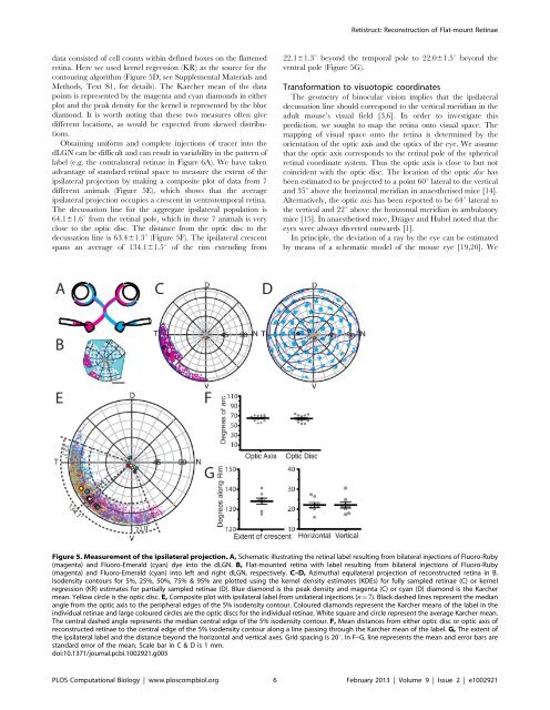
Retistruct: Reconstruction of Flat-mount Retinaedata consisted of cell counts within defined boxes on the flattenedretina. Here we used kernel regression (KR) as the source for thecontouring algorithm (Figure 5D; see Supplemental Materials andMethods, Text S1, for details). The Karcher mean of the datapoints is represented by the magenta and cyan diamonds in eitherplot and the peak density for the kernel is represented by the bluediamond. It is worth noting that these two measures often givedifferent locations, as would be expected from skewed distributions.Obtaining uniform and complete injections of tracer into thedLGN can be difficult and can result in variability in the pattern oflabel (e.g. the contralateral retinae in Figure 6A). We have takenadvantage of standard retinal space to measure the extent of theipsilateral projection by making a composite plot of data from 7different animals (Figure 5E), which shows that the averageipsilateral projection occupies a crescent in ventrotemporal retina.The decussation line for the aggregate ipsilateral population is64.161.6u from the retinal pole, which in these 7 animals is veryclose to the optic disc. The distance from the optic disc to thedecussation line is 63.461.3u (Figure 5F). The ipsilateral crescentspans an average of 134.161.5u of the rim extending from22.161.3u beyond the temporal pole to 22.061.5u beyond theventral pole (Figure 5G).Transformation to visuotopic coordinatesThe geometry of binocular vision implies that the ipsilateraldecussation line should correspond to the vertical meridian in theadult mouse’s visual field [3,6]. In order to investigate thisprediction, we sought to map the retina onto visual space. Themapping of visual space onto the retina is determined by theorientation of the optic axis and the optics of the eye. We assumethat the optic axis corresponds to the retinal pole of the sphericalretinal coordinate system. Thus the optic axis is close to but notcoincident with the optic disc. The location of the optic disc hasbeen estimated to be projected to a point 60u lateral to the verticaland 35u above the horizontal meridian in anaesthetised mice [14].Alternatively, the optic axis has been reported to be 64u lateral tothe vertical and 22u above the horizontal meridian in ambulatorymice [15]. In anaesthetised mice, Dräger and Hubel noted that theeyes were always diverted outwards [1].In principle, the deviation of a ray by the eye can be estimatedby means of a schematic model of the mouse eye [19,20]. WeFigure 5. Measurement of the ipsilateral projection. A, Schematic illustrating the retinal label resulting from bilateral injections of Fluoro-Ruby(magenta) and Fluoro-Emerald (cyan) dye into the dLGN. B, Flat-mounted retina with label resulting from bilateral injections of Fluoro-Ruby(magenta) and Fluoro-Emerald (cyan) into left and right dLGN, respectively. C–D, Azimuthal equilateral projection of reconstructed retina in B.Isodensity contours for 5%, 25%, 50%, 75% & 95% are plotted using the kernel density estimates (KDEs) for fully sampled retinae (C) or kernelregression (KR) estimates for partially sampled retinae (D). Blue diamond is the peak density and magenta (C) or cyan (D) diamond is the Karchermean. Yellow circle is the optic disc. E, Composite plot with ipsilateral label from unilateral injections (n~7). Black dashed lines represent the medianangle from the optic axis to the peripheral edges of the 5% isodensity contour. Coloured diamonds represent the Karcher means of the label in theindividual retinae and large coloured circles are the optic discs for the individual retinae. White square and circle represent the average Karcher mean.The central dashed angle represents the median central edge of the 5% isodensity contour. F, Mean distances from either optic disc or optic axis ofreconstructed retinae to the central edge of the 5% isodensity contour along a line passing through the Karcher mean of the label. G, The extent ofthe ipsilateral label and the distance beyond the horizontal and vertical axes. Grid spacing is 20u. In F–G, line represents the mean and error bars arestandard error of the mean. Scale bar in C & D is 1 mm.doi:10.1371/journal.pcbi.1002921.g005PLOS Computational Biology | www.ploscompbiol.org 6 February 2013 | Volume 9 | Issue 2 | e1002921
Retistruct: Reconstruction of Flat-mount RetinaeFigure 6. Alignment of the binocular zone in visuotopic coordinates. A, Azimuthal equilateral projections in standard retinal space of leftand right retinae with ipsilateral (upper) and contralateral (lower) label resulting from bilateral injections of Fluoro-Ruby (magenta) and Fluoro-Emerald (cyan) into left and right dLGN, respectively, of the same mouse. Plots were generated from stitched 106 epifluorescent images and celllocations detected using ImageJ. For this figure, we have abandoned the convention of always plotting nasal retina to the right. B, Schematicillustrating the approximate projection of retinal space onto visual space. When the orientation of the optic axis (grey line) is optimal, the ipsilateralcrescent is projected entirely to the opposite visual field. Note that due to the refraction in the lens the visual field is estimated to be 180u for eacheye. C–D, Orthographic projections in central visuotopic space of the two ipsilateral retinae in A with optic axis (*) at 64u azimuth; 22u elevation (C)and with optic disc at 60u azimuth; 35u elevation (D). E, Sinusoidal projection of contralateral retinae in B with the optic axis (*) at 64u azimuth; 22uelevation. Labels N, D, T, V indicate the projection of the corresponding pole of the retina. Grid spacing is 15u.doi:10.1371/journal.pcbi.1002921.g006investigated using one such model [20] to determine the deviationof paraxial rays. The schematic eye model is not, however,constructed to account for wide-field rays, so we decided toapproximate the effect of the optics of the eye by making thedeviation of a rays passing through the posterior nodal point of theeye, which is approximately the centre of the eye, proportional tothe ray’s angle of incidence. The constant of proportionality issuch that rays at 90 to the eye will be projected onto the edge ofthe retina, regardless of the retina’s rim angle (see Figure 6B). Themapping of the eye onto visual space is effected by a coordinatetransformation in which first the approximate optics are used toproject points on the retina through the centre of the eye onto anotional large concentric sphere about the eye representing visualspace. Then the locations of the points on this ‘‘celestial’’ sphereare measured in terms of elevation, the angle above the horizontaland azimuth, the angle made between the point’s meridian planeand the zero meridian plane, i.e. the vertical plane containing thelong axis of the mouse. By convention [3,6,14], projections ofvisual space are presented as though the mouse is sitting facing theobserver, so that the azimuth angle is positive in the left visualfield.Using the above conventions to test whether the position of theipsilateral decussation line corresponds to the vertical meridian invisuotopic space, we have transformed the retinotopic location ofipsilateral retinal ganglion cells, following bilateral injections, intohead-centred visuotopic space [21]. To minimise between-animalvariability, we used bilateral injections into the dLGN: injectingFluoro-ruby on one side and Fluoro-emerald on the other side (seeFigure 5A). Figure 6A illustrates the distribution of retrogradelylabelledganglion cells in the ipsilateral (upper plots) and contralateral(lower plots) retinae. For this Figure, we have abandoned thestandard representation of the nasal retina to the right in order toemphasise the mirror-symmetry of the projections. Injection ofFluoro-emerald into the right dLGN leads to label restricted to theventrotemporal crescent in the right retina but widespread labellingin the left retina; a complementary pattern is seen for an injection ofFluoro-ruby into the left dLGN. When the retinal distribution of theipsilateral ventrotemporal crescent neurons is transformed intovisuotopic space using the optic axis coordinates of 64u azimuth and22u elevation [15], and plotted in an orthographic projection of thecentral visual field, the decussation line lines up with the verticalmeridian. These plots have been rotated with 50u elevation toinclude the upper part of the visual field beyond 180u (Figure 6C). If,in contrast, the ipsilateral projection is transformed using the opticdisc coordinates of 60u azimuth and 35u elevation [14], there is anevident visual mismatch between the two decussation lines(Figure 6D). To examine the visuotopic extent of the contralateralprojection in the two eyes, we displayed the data in a sinusoidal mapprojection to include the full visual field through both eyes(Figure 6E). This demonstrates that the decussation pattern in thecontralateral projection is not as sharp as that in in the ipsilateralprojection. Intriguingly, it appears that inferior-central field, a regionthat would be shadowed by the nose, is also under-represented.Given these observations and our group data for optic disclocation (Figure 5E), this indicates a revised optic disc projection of66u azimuth and 25u elevation. Having fixed the location of theeye in visual space, our data on the uncrossed projection predictthat the width of binocular visual field is 52u at its greatest width,slightly larger than the 30–40u of Dräger and Hubel [1], but withinthe range of 50–60u estimated by Rice et al. [22] and ColemanPLOS Computational Biology | www.ploscompbiol.org 7 February 2013 | Volume 9 | Issue 2 | e1002921
Page 1 and 2: Standard Anatomical and Visual Spac
Page 3 and 4: Retistruct: Reconstruction of Flat-
Page 5: Retistruct: Reconstruction of Flat-
Page 9 and 10: Retistruct: Reconstruction of Flat-

Standard Anatomical and Visual Space for the Mouse Retina ...

You also want an ePaper? Increase the reach of your titles

Delete template?

Save as template?