Standard Anatomical and Visual Space for the Mouse Retina ...

More documents

Recommendations

Info

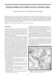
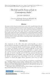
Retistruct: Reconstruction of Flat-mount Retinaeet al. [3]. The binocular field starts a few degrees below thehorizon and continues well behind the animal’s head – very likethe situation in the rabbit [23].Eye muscles and S-opsin in retinal and visuotopiccoordinatesTo examine the orientation of the eye, the locations of theinsertions of superior, lateral and inferior rectus into the globe ofthe eye were marked onto the retina (Figure 7A; see SupplementalMaterials and Methods, Text S1, for procedure). The nasal pole ofthe retinae is determined with reference to the nictitatingmembrane. The retinae were reconstructed and plotted in anazimuthal equidistant polar projection and the vectors connectingthe insertion points and the optic disc were plotted (Figure 7B).Once in a standard space, the muscle insertion points (n~33) fromall the retinae (n~17) were plotted in the same plot and thevectors connecting the Karcher mean of each muscle insertion andthe Karcher mean for the optic disc location were plotted(Figure 7C). Figure 7D shows the mean vector angles: lateralrectus, at 184.963.6u, is directly opposite the nasal cut, superiorrectus is at 91.365.9u and inferior rectus is at 284.264.1u,wherenasal is 0u. It is noticeable that there is considerable variability inthe locations of the muscle insertions, certainly when compared tothe variability of the optic discs. A considerable contributory factorin this is the large extent of the muscle and the relative difficulty indetermining the centre of the muscle.The location of the optic axis at 64u azimuth and 22u elevation[15] determines the location of the vertical and horizontalmeridians on the eye. The location of the ipsilateral decussationline confirms this azimuthal value (Figures 5E & 6C). As the mouseretina has no pronounced horizontal streak, we looked at thedistribution of short wavelength opsin (S-opsin) in the retina.Haverkamp et al. [24] describe a very distinct distribution patternin the retina, with high density ventral, low density dorsal and anabrupt transition and suggested that the transition coincided withthe horizontal meridian. Figure 8A shows immuno-staining for S-opsin from dorsal, central and ventral retina. The densitydifference between dorsal and ventral is marked and the transitionis abrupt. Figure 8B & 8C illustrate the transformation of the S-opsin distribution from retinal flat-mounts to standard retinalspace to an orthographic representation of visuotopic spacecentred on the optic axis. In these plots, the transition is3.360.3u above the horizontal meridian at the level of the opticaxis and is tilted by 13.863.6u, so that transition is 7.862.0u abovethe horizontal meridian in central visual field and 6.061.6u belowthe horizontal meridian peripherally (Figure 8D). The label fromboth left and right retinae was also plotted in a sinusoidalprojection (Figure 8D) to illustrate that the rotation seen in theorthogonal plots for each eye is symmetric along the verticalmeridian of the entire visual field (Figure 8E).In summary, with the location of the optic axis determined bythe optimal match of the decussation line with the verticalmeridian, the change in S-opsin staining nicely coincides with thehorizontal meridian, at least for the central visual field, aspredicted by Szél et al. [25]. It is worth noting that S-opsin ismostly co-expressed with medium wavelength opsin (M-opsin)[24,26], and that this would make these cones in upper visual fieldrespond to a broader spectrum, which may have implications forthe ability to detect a larger range of objects above the mouse. Theprecise distribution of S-opsin is not uniformly agreed upon [24–26]. However, when plotting the distributions from Szél et al [25]to visuotopic space using Retistruct (data not shown), we get a verysimilar distribution to that seen in Figure 8B–C.Figure 7. Measurement of muscle insertion angles. A, Flatmountedretina showing stitching and insertions for superior rectus(red), lateral rectus (green) and inferior rectus (blue). N indicates nasalcut. Plots on right represent the distortions introduced by reconstructingretina (see Figure 2 for explanation). B, Azimuthal equilateralprojection of reconstructed retina in A. Dashed lines represent vectorsconnecting muscle insertion point to the optic disc. C, Muscle insertionpoints from 17 retinae. Solid black circles represent the optic discs forindividual retinae. Dashed lines represent the line from each individualinsertion point to its respective optic disc. Solid lines are from theKarcher mean insertion to the Karcher mean location of the optic disc.Grid Spacing is 15u. D, Plot of the angles of the angles of vectorsconnecting muscle insertions of Superior Rectus (SR), Lateral Rectus (LR)and Inferior Rectus (IR) to the individual optic discs. Bar represents themean and error-bars are standard deviation.doi:10.1371/journal.pcbi.1002921.g007Availability and Future DirectionsThe reconstruction and transformation methods described herehave been implemented in R [27] and use the Triangle library[28] for mesh generation. The retinae in this paper werereconstructed and analysed using version 0.5.7 of the Retistructpackage (Dataset S1). The package, including full installationinstructions, is also available anonymously and for free under theGPL license from http://retistruct.r-forge.r-project.org/. Thepackage has been tested with R version 2.15.2 on GNU/Linux(Ubuntu 12.04), MacOS X 10.8 and Microsoft Windows Vista.The user guide, available from the same site, contains details of thetwo main data formats Retistruct can process. These are either inthe form of coordinates of data points and retinal outline from anin-house camera-lucida setup, or in the form of bitmap imageswith an outline marked up in ImageJ ROI format [29]. There is aGUI interface to facilitate the marking-up of retinae anddisplaying reconstructed retinae.The program could be applied to flat-mount preparations ofretinae from any vertebrate species at any age, provided the globeof the eye is approximately spherical, and it would be possible toadd extra analysis routines. When examining retinae with mosaiclabelling [30], reconstructing the retina into its original sphericalcoordinates would make it possible to determine more accuratelythe relative distances between cells between peripheral and centralretina. To implement mosaic analysis would require computationof a Voronoi tessellation on the sphere, which could beimplemented by doing the Voronoi tessellation on a conformal(Wulff) projection [31]. Further visualisation methods could alsoPLOS Computational Biology | www.ploscompbiol.org 8 February 2013 | Volume 9 | Issue 2 | e1002921
Retistruct: Reconstruction of Flat-mount RetinaeFigure 8. Visuotopic axes with respect to S-opsin distribution. A, S-opsin staining in dorsal, central and ventral retina. Images acquired at206magnification. Scale bar is 100 m. B–C, S-opsin distribution for right (A) and left (B) eyes plotted in orthographic projection centred on optic axis(*) at 22u elevation and 64u azimuth. Bottom left plot is flat-mounted retina. Bottom right plot is azimuthal equilateral plot. Plots were generated fromstitched 106 epifluorescent images and cell locations detected using ImageJ [29]. There are slight differences between the two eyes in the exactangle of density transition with respect to the horizontal meridian and in the density of staining around the optic disc. These will reflect experimentalvariance. Again our normal convention of showing nasal to the left has been relaxed. Scale bar is 1 mm. D, The average offset of the S-opsin densitytransitionfrom the horizontal meridian in central and peripheral visual field (n~9). Error bars are SEM. E, S-opsin distribution for both eyes plotted ina sinusoidal projection with same optic axis (*) as in C. Yellow outline is edge of left retina; red outline is edge of right retina. Labels N, D, T, V indicatethe projection of the corresponding pole of the retina. Grid spacing is 15u.doi:10.1371/journal.pcbi.1002921.g008be added. Using equations similar to those in the literature [21],locations on the retina could be projected onto a screen placedorthogonal to the optic axis, thus enabling a direct translation ofvisual stimulus space onto retinal coordinates. It would also bepossible to map visual space onto retinal coordinates, by invertingthe operations to map the retina onto visual space.It should be stressed that the current version is not intended foruse on partial retinae. However, it might eventually be possible tolocate incomplete retinae in standard retinal space, if there enoughmarkers to orient the partial retina correctly. Similarly, it shouldbe possible to locate sections (either histological or tomological) ofknown orientation and hemiretinal origin in standard space.Supporting InformationDataset S1 Complete source code for the Retistruct package(version 0.5.7). Includes demonstration data for Figures 1, 2 and 6in this paper, a user guide with installation instructions, and areference manual containing descriptions of the functions used inthe package.(ZIP)References1. Dräger UC, Hubel DH (1976) Topography of visual and somatosensoryprojections to mouse superior colliculus. J Neurophysiol 39: 91–101.2. McLaughlin T, O’Leary DD (2005) Molecular gradients and development ofretinotopic maps. Annu Rev Neurosci 28: 327–355.3. Coleman JE, Law K, Bear MF (2009) Anatomical origins of ocular dominance inmouse primary visual cortex. Neuroscience 161: 561–571.Text S1 Supplemental information including an extendedDiscussion, and Materials and Methods containing details ofexperiments and detailed description of the reconstructionalgorithm and analysis of reconstructed data.(PDF)AcknowledgmentsThe authors would like to thank Andrew Lowe, Stephen Eglen, Johannes J.J. Hjorth, and Michael Herrmann for their very helpful commentsthroughout this work. We would also like to thank Nicholas Sarbicki forhelping with the analysis of LGN projections and Henry Eynon-Lewis forassistance with dissections for muscle-insertion marking and S-opsinstaining. We thank anonymous reviewers for alerting us to futurepossibilities of using Retistruct to map partial or sectioned retinae ontostandard retinal space.Author ContributionsConceived and designed the experiments: DCS DL IDT. Performed theexperiments: DL IDT. Analyzed the data: DCS DL IDT. Contributedreagents/materials/analysis tools: DCS. Wrote the paper: DCS DL DJWIDT. Wrote the software package: DCS.4. Reber M, Burrola P, Lemke G (2004) A relative signalling model for theformation of a topographic neural map. Nature 431: 847–853.5. Rashid T, Upton AL, Blentic A, Ciossek T, Knöll B, et al. (2005) Opposinggradients of ephrin-As and EphA7 in the superior colliculus are essentialfor topographic mapping in the mammalian visual system. Neuron 47: 57–69.PLOS Computational Biology | www.ploscompbiol.org 9 February 2013 | Volume 9 | Issue 2 | e1002921
Page 1 and 2: Standard Anatomical and Visual Spac
Page 3 and 4: Retistruct: Reconstruction of Flat-
Page 5 and 6: Retistruct: Reconstruction of Flat-
Page 7: Retistruct: Reconstruction of Flat-

Standard Anatomical and Visual Space for the Mouse Retina ...

You also want an ePaper? Increase the reach of your titles

Delete template?

Save as template?