- Page 1:
Fast Automatic Unsupervised Image S
- Page 5:
In presenting this dissertation in
- Page 9 and 10:
TABLE OF CONTENTSList of FiguresLis
- Page 11 and 12:
4.1.2 Penalty Adjustment . . . . .
- Page 13 and 14:
Appendix A: Software Discussion 169
- Page 15 and 16:
4.1 (a) Signal generated by an AR(1
- Page 17 and 18:
5.29 Aerial image of a buoy, before
- Page 19:
DEDICATIONThis work is dedicated to
- Page 22 and 23:
20 10 20 30 40 50 600 10 20 30 40 5
- Page 24 and 25:
4fast because they can be implement
- Page 26 and 27:
6multidimensional observations at e
- Page 28 and 29:
••••8Figure 2.1(a) is a sim
- Page 30 and 31:
10Principal Curve•••••Dat
- Page 32 and 33:
12based on the estimates of the par
- Page 34 and 35:
14first of these can be done by a h
- Page 36 and 37:
162.4 Examples2.4.1 A Simulated Two
- Page 38 and 39:
18Figure 2.5: HPCC applied to the t
- Page 41 and 42:
21Table 2.2: BIC results for simula
- Page 43 and 44:
232.4.3 New Madrid Seismic RegionDa
- Page 45 and 46:
25Table 2.3: BIC results for New Ma
- Page 47 and 48:
27Latitude35.5 36.0 36.5 37.0 37.5
- Page 49 and 50:
29set, so we want to avoid assumpti
- Page 51 and 52:
31The examples we have presented in
- Page 53 and 54:
Chapter 3MARGINAL SEGMENTATIONIn th
- Page 55 and 56:
35about ˜θ; this is a good approx
- Page 57 and 58:
373.2 Mixture ModelsThe mixture den
- Page 59 and 60:
39for estimating the model paramete
- Page 61 and 62:
41The ith pixel of X or C is denote
- Page 63 and 64:
43In componentwise classification,
- Page 65 and 66:
45ponent. This classification proce
- Page 67 and 68:
Chapter 4ADJUSTING FOR AUTOREGRESSI
- Page 69 and 70:
49Dependence CaseWhen |β| < 1, the
- Page 72 and 73:
52For practical purposes, equation
- Page 74 and 75:
54g ′′ (θ) ≈⎛⎜⎝∑ Ni=
- Page 76 and 77:
564.1.3 Computing BIC with the AR(1
- Page 78 and 79:
58upper, left, and right borders of
- Page 80 and 81:
60L(Y −B |M, B) = L IND (Y −B |
- Page 82 and 83:
62We now return to equation 4.56 an
- Page 84 and 85:
64and then computing a mean-correct
- Page 86 and 87:
66regression, which can be written
- Page 88 and 89:
68resulting R 2 values are 0.93 for
- Page 90 and 91:
700 5 10 15 200 5 10 15 20Figure 4.
- Page 92 and 93:
72negative value would mean that ne
- Page 94 and 95:
74Once each pixel has been updated,
- Page 96 and 97:
76The basic idea of this psuedolike
- Page 98 and 99:
78The consistency result presented
- Page 100 and 101:
80⎛∑ ⎞Kj=1f(Yg i (Y i ) = log
- Page 102 and 103:
82| log(f(Y i |X i = S, θ 1 ))|
- Page 104 and 105:
84⇒ (L ˆX (Y |K)) exp(−(D K
- Page 106 and 107:
86the object of the expectation is
- Page 108 and 109:
88Thus, equation 5.42 holds, so BIC
- Page 110 and 111:
90the inequality in equation 5.55 h
- Page 112 and 113:
92N log(σ K ) − N log(σ 1 ) −
- Page 114 and 115: 94final number of clusters. The cho
- Page 116 and 117: 96ization to initialize (see sectio
- Page 118 and 119: 98ˆσ 2 j =∑ Ni=1 ˆQ ij (Y i
- Page 120 and 121: 100one particular data value, which
- Page 122 and 123: 102classification they are not. Eac
- Page 124 and 125: 1045.2.6 Morphological Smoothing (O
- Page 126 and 127: 1065.3 Image Segmentation Examples5
- Page 128 and 129: 1080 10 20 30 400 10 20 30 40Figure
- Page 130 and 131: 1100.0 0.005 0.010 0.015 0.020 0.02
- Page 132 and 133: 112three pixels remain incorrectly
- Page 134 and 135: 114Table 5.3: EM-based parameter es
- Page 136 and 137: 1160 10 20 30 40 50 600 10 20 30 40
- Page 138 and 139: 1180 10 20 30 40 50 600 10 20 30 40
- Page 140 and 141: 1205.3.3 Ice FloesFigure 5.10 shows
- Page 142 and 143: 1220 20 40 60 80 1000 20 40 60 80 1
- Page 144 and 145: 124Percent0.0 0.005 0.010 0.015 0.0
- Page 146 and 147: 1260 20 40 60 80 1000 20 40 60 80 1
- Page 148 and 149: 1280 20 40 60 80 1000 20 40 60 80 1
- Page 150 and 151: 1305.3.4 Dog LungFigure 5.17 presen
- Page 152 and 153: 132Table 5.6: Logpseudolikelihood a
- Page 154 and 155: 134Percent0.0 0.05 0.10 0.15 0.200
- Page 156 and 157: 1360 20 40 60 80 100 1200 20 40 60
- Page 158 and 159: 1380 20 40 60 80 100 1200 20 40 60
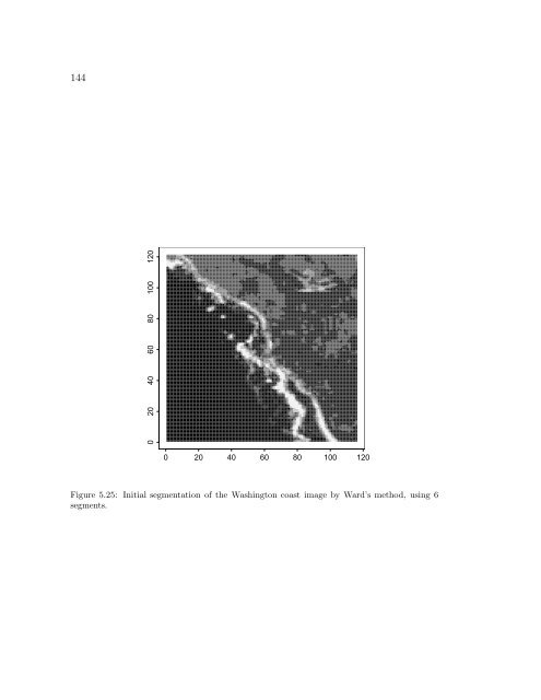
- Page 160 and 161: 140interior to the land which had i
- Page 162 and 163: 142Table 5.9: EM-based parameter es
- Page 166 and 167: 1460 20 40 60 80 100 1200 20 40 60
- Page 168 and 169: 1485.3.6 BuoyFigure 5.29 is an aeri
- Page 170 and 171: 150Table 5.10: Logpseudolikelihood
- Page 172 and 173: 1520 20 40 60 80 1000 20 40 60 80 1
- Page 174 and 175: 1540 20 40 60 80 1000 20 40 60 80 1
- Page 176 and 177: 1560 20 40 60 80 1000 20 40 60 80 1
- Page 178 and 179: Chapter 6CONCLUSIONSThis dissertati
- Page 180 and 181: 160of subsampling would have to be
- Page 182 and 183: REFERENCESAllard, D., and Fraley, C
- Page 184 and 185: 16494, 555-568.Fraley, C., and Raft
- Page 186 and 187: 166Maps,” Biological Cybernetics,
- Page 188 and 189: 168Zahn, C. (1971), “Graph-Theore
- Page 190 and 191: 170structuring element file.Segment
- Page 192 and 193: 172A.3 Splus codehpcc - Hierarchica
- Page 194: VITA1993 B.S. Mathematics, Harvey M