View - Statistics - University of Washington

More documents

Recommendations

Info

21Table 2.2: BIC results for simulated sine wave minefield.DF 0 Features 1 Feature 2 Features 3 Features2 -1031 -1034 -1018 -9913 -1031 -1016 -938 -9414 -1031 -975 -889 -9085 -1031 -911 -883 -9046 -1031 -884 -887 -9017 -1031 -873 -894 -9018 -1031 -868 -901 -9079 -1031 -869 -908 -92110 -1031 -872 -913 -92911 -1031 -873 -919 -94012 -1031 -877 -926 -951Figure 2.7: Simulated curvilinear minefield after denoising using nearest neighbor cleaning.
Page 1: Fast Automatic Unsupervised Image S
Page 5: In presenting this dissertation in
Page 9 and 10: TABLE OF CONTENTSList of FiguresLis
Page 11 and 12: 4.1.2 Penalty Adjustment . . . . .
Page 13 and 14: Appendix A: Software Discussion 169
Page 15 and 16: 4.1 (a) Signal generated by an AR(1
Page 17 and 18: 5.29 Aerial image of a buoy, before
Page 19: DEDICATIONThis work is dedicated to
Page 22 and 23: 20 10 20 30 40 50 600 10 20 30 40 5
Page 24 and 25: 4fast because they can be implement
Page 26 and 27: 6multidimensional observations at e
Page 28 and 29: ••••8Figure 2.1(a) is a sim
Page 30 and 31: 10Principal Curve•••••Dat
Page 32 and 33: 12based on the estimates of the par
Page 34 and 35: 14first of these can be done by a h
Page 36 and 37: 162.4 Examples2.4.1 A Simulated Two
Page 38 and 39: 18Figure 2.5: HPCC applied to the t
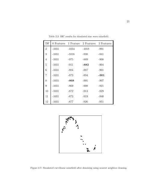
Page 42 and 43: 22Figure 2.8: Initial clustering of
Page 44 and 45: 24Latitude35.5 36.0 36.5 37.0 37.5
Page 46 and 47: 26Latitude35.5 36.0 36.5 37.0 37.5
Page 48 and 49: 282.5 DiscussionWe have introduced
Page 50 and 51: 30transform type of approach. The e
Page 52 and 53: 32curve. Extending the method to ac
Page 54 and 55: 34is to use a likelihood ratio test
Page 56 and 57: 36The error of the approximation in
Page 58 and 59: 38the image with this independence
Page 60 and 61: 403.4.1 Mixture versus Componentwis
Page 62 and 63: 42P (X i = m|Y i ) ∝ P (Y i |X i
Page 64 and 65: 44In finding argmax C g(C|X), we ca
Page 66 and 67: 46fine tuning of this. For instance
Page 68 and 69: 48is σ 2 Y .Independence CaseWhen
Page 70: 50L(Y −1 |M, Y 1 ) = − N − 12
Page 73 and 74: 53analysis. We now consider g ′
Page 75 and 76: 55g(θ) ≈ log(p(Y |θ, M)) (4.38)
Page 77 and 78: 574.2 Adjusting BIC for the Raster
Page 79 and 80: 59ˆσ 2 ɛ = 1N 0 − 1∑(Y i −
Page 81 and 82: 61E[(Y i − µ)(Y (i−j) − µ)]
Page 83 and 84: 63The dependence model uses additio
Page 85 and 86: 65(BIC(K) = 2 L IND (Y −B | θ ˆ
Page 87 and 88: 67number of pixels minus the number
Page 89 and 90: 69in figure 4.1B). This problem cau
Page 91 and 92:
Chapter 5AUTOMATIC IMAGE SEGMENTATI
Page 93 and 94:
73the Gaussian parameters ˆθ, whi
Page 95 and 96:
75f( ˆX|Y, ˆφ, ˆθ) ∝ ∏ if(
Page 97 and 98:
77After running ICM, we have an est
Page 99 and 100:
79denoted by µ K and σK; 2 equati
Page 101 and 102:
81∫ ∞−∞|g i (Y i )|f(Y i )d
Page 103 and 104:
83Lemma 2: ErgodicityLet X = X i ,
Page 105 and 106:
85both dimensions) we are asymptoti
Page 107 and 108:
87⎛∑ Kj=1f(YE KT⎝i |X i = j,
Page 109 and 110:
89⎛∑ ∑ KTlog ⎝ j=1 f(Y i |X
Page 111 and 112:
91− ∑ (Y i − µ 2 ) 2i∈S 22
Page 113 and 114:
935.2 An Automatic Unsupervised Seg
Page 115 and 116:
95has at least T 0 pixels. The proc
Page 117 and 118:
97is the number of components (this
Page 119 and 120:
99ˆµ j =∑ Ci=1H i ˆR ij V i∑
Page 121 and 122:
101However, experience with the EM
Page 123 and 124:
103log L ˆX (Y |K) = ∑ ilog(f(Y
Page 125 and 126:
105operation. Then erosion can be e
Page 127 and 128:
107is found; this results in a much
Page 129 and 130:
1090 10 20 30 400 10 20 30 40Figure
Page 131 and 132:
1115.3.2 Simulated Three Segment Im
Page 133 and 134:
1130 10 20 30 40 50 600 10 20 30 40
Page 135 and 136:
115Percent0.0 0.002 0.004 0.006 0.0
Page 137 and 138:
1170 10 20 30 40 50 600 10 20 30 40
Page 139 and 140:
1190 10 20 30 40 50 600 10 20 30 40
Page 141 and 142:
121only one possible melt pool is e
Page 143 and 144:
123Table 5.5: EM-based parameter es
Page 145 and 146:
1250 20 40 60 80 1000 20 40 60 80 1
Page 147 and 148:
1270 20 40 60 80 1000 20 40 60 80 1
Page 149 and 150:
1290 20 40 60 80 1000 20 40 60 80 1
Page 151 and 152:
131artifacts as well.The ICM refine
Page 153 and 154:
133Table 5.7: EM-based parameter es
Page 155 and 156:
1350 20 40 60 80 100 1200 20 40 60
Page 157 and 158:
1370 20 40 60 80 100 1200 20 40 60
Page 159 and 160:
1395.3.5 Washington CoastFigure 5.2
Page 161 and 162:
141Table 5.8: Logpseudolikelihood a
Page 163 and 164:
143Percent0.0 0.02 0.04 0.06 0.080
Page 165 and 166:
1450 20 40 60 80 100 1200 20 40 60
Page 167 and 168:
1470 20 40 60 80 100 1200 20 40 60
Page 169 and 170:
149visible, both in jagged horizont
Page 171 and 172:
151Table 5.11: EM-based parameter e
Page 173 and 174:
153Percent0.0 0.02 0.04 0.06 0.080
Page 175 and 176:
1550 20 40 60 80 1000 20 40 60 80 1
Page 177 and 178:
1570 20 40 60 80 1000 20 40 60 80 1
Page 179 and 180:
159The image segmentation examples
Page 181 and 182:
161to provide predictive inference
Page 183 and 184:
163Campbell, N.W., Mackeown, W.P.J.
Page 185 and 186:
165Hartigan, J. A. (1975). Clusteri
Page 187 and 188:
167Prim, R. (1957), “Shortest Con
Page 189 and 190:
Appendix ASOFTWARE DISCUSSIONA.1 XV
Page 191 and 192:
171emoutput.txt, emimageout.pgm.emn
Page 193 and 194:
173unique data values, so it can ha
show all

View - Statistics - University of Washington

Create successful ePaper yourself

Delete template?

Save as template?