Enrichment of Radon and Carbon Dioxide in the Open Atmosphere ...

Articlepubs.acs.org/estEnrichment of Radon and Carbon Dioxide in the Open Atmosphereof an Australian Coal Seam Gas FieldDouglas R. Tait, †, * Isaac R. Santos, † Damien T. Maher, † Tyler J. Cyronak, † and Rachael J. Davis †† Centre for Coastal Biogeochemistry, School of Environment, Science and Engineering, Southern Cross University, PO Box 157,Lismore, NSW, Australia, 2480ABSTRACT: Atmospheric radon ( 222 Rn) and carbon dioxide (CO 2 ) concentrationswere used to gain insight into fugitive emissions in an Australian coal seamgas (CSG) field (Surat Basin, Tara region, Queensland). 222 Rn and CO 2concentrations were observed for 24 h within and outside the gas field. Both222 Rn and CO 2 concentrations followed a diurnal cycle with night timeconcentrations higher than day time concentrations. Average CO 2 concentrationsover the 24-h period ranged from ∼390 ppm at the control site to ∼467 ppm nearthe center of the gas field. A ∼3 fold increase in maximum 222 Rn concentration wasobserved inside the gas field compared to outside of it. There was a significantrelationship between maximum and average 222 Rn concentrations and the numberof gas wells within a 3 km radius of the sampling sites (n = 5 stations; p < 0.05). Apositive trend was observed between CO 2 concentrations and the number of CSGwells, but the relationship was not statistically significant. We hypothesize that theradon relationship was a response to enhanced emissions within the gas field related to both point (well heads, pipelines, etc.)and diffuse soil sources. Radon may be useful in monitoring enhanced soil gas fluxes to the atmosphere due to changes in thegeological structure associated with wells and hydraulic fracturing in CSG fields.■ INTRODUCTIONThe past decade has seen a dramatic increase in unconventionalgas extraction worldwide. Unconventional gas differs fromconventional gas in that conventional gas is trapped in naturalpores or fractures in sedimentary layers while unconventionalgas can also be adsorbed to the sediment itself. One of theseunconventional gases is coal seam gas (CSG), also known ascoal bed methane. Production of CSG relies on the extractionof water, which reduces pore pressures and thereby allows gasesto desorb and flow through fractures and micropores in a coalseam. Technological advances such as directional drilling andhydraulic fracturing (i.e., the injection of fluid and proppantsunder pressure into the wellbore to fracture geological strata),have allowed greater access to these gas reserves throughincreasing the connective matrix in subsurface sediments. Initialstudies have shown that unconventional shale gas extractionmay increase groundwater−methane concentrations in thevicinity of gas production wells. 1 However, there is also thepotential for unintentional or “fugitive” emissions producedthrough the CSG mining process to be released into theatmosphere.Fugitive emissions are gases that are unintentionally lost tothe atmosphere through the gas extraction, collection,processing and transportation processes. These emissions canemanate from point sources (e.g., venting, equipment leaks, anddistribution) and enhanced diffusion of gas from soils.Emissions include greenhouse gases (GHG) such as carbondioxide (CO 2 ) and methane (CH 4 ). While not harmful tohuman health at low concentrations, these emissions should beaccounted for when estimating the net greenhouse gas footprintof CSG operations. The release of methane is of particularinterest as it is a powerful greenhouse gas with a global warmingpotential 25 times that of CO 2 over a 100-year time horizon. 2Importantly, the atmospheric presence of these gases maysuggest the release of other gaseous substances, such as volatileorganic carbons 3,4 which may be harmful to human health. 5Without a quantitative knowledge of the gases produced andtheir sources and sinks, it is difficult to unequivocally estimategas fluxes through modeling approaches. 6Monitoring of radon ( 222 Rn) has been undertaken fordecades in enclosed spaces such as mines and dwellings wherethe build-up of the gas can be harmful to human health. 7Enhanced radon concentrations in groundwater and theatmosphere have also been linked to earthquakes. 8 Radon is aradioactive (half-life = 3.84 days) noble gas that is produced inthe 238 U decay chain. 9,10 Since uranium is present in nearly allrocks and sediments, soil-gas exchange represents a nearlycontinuous source of radon to the atmosphere. Radon is anexcellent natural soil gas tracer because it is unreactive and itsshort half-life prevents any significant build-up in theatmosphere over long time scales. Therefore, the presence of222 Rn in the atmosphere requires a nearby source. In addition,Received: November 7, 2012Revised: February 21, 2013Accepted: February 27, 2013Published: February 27, 2013© 2013 American Chemical Society 3099 dx.doi.org/10.1021/es304538g | Environ. Sci. Technol. 2013, 47, 3099−3104

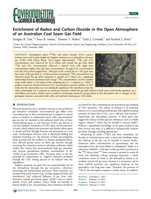
Environmental Science & TechnologyArticleFigure 1. The study site in the Surat Basin, Tara region, Queensland. Gas wells are indicated by a red cross (data from http://mines.industry.qld.gov.au/geoscience/interactive-resource-tenure-maps.htm, accessed 24 October 2012). The red crosses may represent more than one well if they are inclose proximity. CO 2 (ppm) and 222 Rn (Bq m −3 ± 2σ) concentrations over a ∼24-h period are indicated for each site. The gray areas representnight-time, while the white areas represent daytime.■radon can be easily detected by portable instruments that can EXPERIMENTAL SECTIONbe deployed in the field.We hypothesize that measurement of atmospheric 222 This study was performed in a CSG field near Tara,RnQueensland, Australia (∼26°50′0″S, 150°20′0″E). The areaconcentrations may provide a simple and effective way to gaininsight into fugitive emissions from CSG mining activities. Thehas two main gas fields, the Talinga and the Kenya gas fields,aim of this study was to assess whether atmospheric 222 Rn andwith wells in varying states of exploration and production. TheCO 2 concentrations are enriched within an Australian CSG production and exploration of CSG in the area is associatedfield relative to nearby areas outside the CSG field. We with the extensive Walloon Coal Measures, which are relativelypostulate that a relationship between gas concentrations and permeable (>4.93 x10 −13 m 2 in some seams) and generallythe number of nearby CSG wells will emerge if CSG extraction shallow (near surface to

Environmental Science & TechnologyWe deployed 24-h time-series stations to measure atmospheric222 Rn and CO 2 at three locations within the gas fieldsand two stations outside of the gas fields (Figure 1). A gasintake was positioned at 2 m above the ground at each station.The first station (hereafter referred to as North) was adjacentto an open wheat field approximately 3 km north of the Kenyagas field and to the east of the Talinga gas field. The second sitewas located on a roadside reserve in the central part of theKenya gas field (Central). The third site was located directlysouth of a large water holding pond in the Kenya gas field(East). The fourth site was located approximately 3 km south ofthe Kenya gas field (South). The fifth site was locatedapproximately 8 km from the southern boundary of the Kenyagas field (Control). For each site, the distance to the nearestwell and the number of nearby wells are indicated in Table 1.Table 1. Position and Proximity of Sampling Sites to CSGWell Heads asitenorthcentraleastsouthcontrollat/long26° 53′S,150° 24′E26° 57′S,150° 25′E26° 57′S,150° 28′E27° 1′S,150° 27′E27° 5′S,150° 20′E∼distance tonearest gas well(m)1(km)wells within2(km)3(km)4(km)60 4 15 27 51500 4 17 36 63250 1 9 19 271500 0 2 5 74400 0 0 0 0a The location of well heads was obtained from www.mines.industry.qld.gov.au/geoscience/interactive-resource-tenure-maps.htm, accessed24 October 2012.Measurements of 222 Rn concentrations were performed usinga commercially available continuous radon-in-air monitor(RAD-7, Durridge Company), with two-hour averagingintervals to ensure acceptable counting statistics. CO 2 measurementswere taken using two nondispersive infrared gasanalysers (Li-cor 820) and two nondispersive differential gasanalysers (Li-cor 7000) recording at one minute intervals.Water vapor was removed from air sample streams using aDrierite column in-line with the analysers. All CO 2 analyserswere calibrated using 0 and 502 ± 10 ppm certified referencegases (Coregas Australia). The uncertainty of individual CO 2detectors was less than 2%, well below the natural variability inthe region. For CO 2 concentrations at the South site and thefinal 12 h at the Control site, CO 2 was measured every fourhours using a cavity ringdown spectrometer (Picarro G2201-iCRDS). The spectrometer calibration was within 10 ppm of theLi-cor CO 2 analysers. The radon monitors were calibrated bythe manufacturer (±5%). A cross-calibration check just beforedeployment resulted in agreement within the calibrationuncertainty. Automated weather stations (Davis Vantage Pro)were deployed on six-meter poles at the South and Controlsites to determine wind, temperature and humidity fluctuations.To compare averages, one-way ANOVA and regressionanalyses were done using SPSS with p values ≤0.05 consideredsignificant.3101■ArticleRESULTS AND DISCUSSIONTime Series Observations. Calm winds occurred duringour experiment. During the day, winds were predominantlyfrom the NNE and averaged ∼1.2 m s −1 . At night, wind speedsapproached zero. Over the 24 h period, temperatures rangedfrom 10 to 25 °C. Humidity ranged from 25% during the day to90% at night. There was no significant difference in the averageatmospheric pressure during the day and night (1008.5 ± 3.9mbar and 1008.9 ± 1.1 mbar respectively).Concentrations of 222 Rn and CO 2 followed similar diurnalpatterns with lower concentrations during daylight hours(Figure 1). CO 2 concentrations varied from day to night byover 60 ppm at the Central site and by as little as 5 ppm at theControl site. Concentrations of 222 Rn increased at night by ∼5fold at the Central and South sites and approximately doubledat the Control site. This is probably due to the formation of atemperature inversion layer at night, trapping any emissionscloser to the surface and causing the accumulation of gasesreleased from soils or CSG infrastructure. The release of radonat the soil-air interface has been shown to follow a diurnalpattern with variations governed by temperature and windspeeds, 13 which is consistent with our observations. The effectsof night-time inversion layers on 222 Rn concentrations has beenpreviously described for non-CSG regions. 14 Lower windspeeds and a lower atmospheric mixing height at night mayallow the accumulation of soil gas in the atmosphere. These areimportant considerations for assessing CSG fugitive emissionsas the time of sampling could significantly alter theconcentration of gases in the atmosphere, and as such samplingof full 24-h cycles is essential. A distinct spike in CO 2 and 222 Rnconcentrations occurred at the Central site approximately 13.5to 15 h after the start of monitoring. This spike correspondedto a distinct shift in winds from NNE at ∼1.3 m s −1 to easterlyat ∼0.5 m s −1 before returning to a NNE direction.The highest average CO 2 concentration during the 24-hperiod was measured at the Central site (∼468 ppm) while thelowest was at the Control site (∼391 ppm) (Figure 2). ThereFigure 2. Average CO 2 (a) and 222 Rn (b) concentrations ±1 SDatdifferent sampling sites. The maximum CO 2 (a) and 222 Rn (b)concentrations during the day and night are indicated with a solidcircle.dx.doi.org/10.1021/es304538g | Environ. Sci. Technol. 2013, 47, 3099−3104

Environmental Science & Technologywere significantly higher night-time average CO 2 concentrationsat sites within the gas field (North, Central and East)(p < 0.01) than at sites outside (South and Control), while theCentral and East sites had significantly higher CO 2 concentrationsduring the day compared to the other sites (p < 0.01).The only significant difference in 222 Rn concentrations betweensites occurred at night between the Central site and the Controlsite (p = 0.04). This was caused by the relatively large standarddeviations due to the steady increase in 222 Rn concentrationsduring the night coupled with the long averaging times used (2h).Correlations between Gas Concentrations and Numberof CSG Wells. There was a significant relationshipbetween the number of wells within 3 km of sampling sites andthe maximum radon concentration over the 24 h period (r 2 =0.81, p = 0.04) (Figure 3a). If we use the average radonFigure 3. Regression plots of the number of CSG wells within 3 km ofstudy sites and maximum 222 Rn (a), average 222 Rn (b), maximum CO 2(c), and average CO 2 (d) concentrations. Control (Co), South (S),East (E), North (N), and Central (Ce) study sites are indicated.concentration, then the r 2 value is higher (r 2 = 0.87, p = 0.02)(Figure 3b). It is difficult to estimate the exact area influencinggas concentrations at each station. If we use the number ofwells within 1 km, then the correlations illustrated in Figure 3aare weaker (r 2 = 0.74, p = 0.06), while if we use the number ofwells within 4 km of each monitoring station, the correlationsare similar but slightly lower (r 2 = 0.83, p = 0.03). There was nosignificant relationship between the number of wells at 3 kmand the average day (r 2 = 0.30, p = 0.34) and average night (r 2 =0.65, p = 0.10) 222 Rn concentrations largely due to the 222 Rnconcentrations at the south site being comparably low duringthe day (1.48 ± 1.07 bq m −3 ) and high at night (11.21 ± 4.17bq m −3 ).There was a positive, but statistically nonsignificant relationshipbetween the number of wells within 3 km of samplingstations and the maximum CO 2 concentration at each station(r 2 = 0.72, p = 0.07) (Figure 3c). A weaker (but still positive)correlation was found when the average CO 2 concentration ateach site was used (r 2 = 0.56, p = 0.14) (Figure 3d). TheCentral site, which had the highest CO 2 concentrations, waslocated approximately 30 m from a service road in the centralpart of the Kenya gas field (Central). No short-term CO 2 spikessimilar to what would be expected from passing vehicles wasobserved. The relatively low concentrations of CO 2 at theArticleNorth site may be partially due to the location of the station inrelation to the prevailing wind direction. The North site had amuch smaller number of wells upwind compared to the Centralsite. However, similar patterns of low 222 Rn concentrations atthe North site were not observed. The diurnal variations inCO 2 concentrations was likely driven by ecosystem metabolism,leading to a reduction in CO 2 through plant uptake during theday and an increase in CO 2 at night due to respiration. Therelatively higher background CO 2 concentration in theatmosphere associated with a longer residence time thanradon may also have prevented stronger correlations fromemerging as a larger source could be needed to significantlyalter CO 2 concentrations in the atmosphere. CO 2 is only asmall fraction (98% of Walloon CoalCSG 16 ) may be oxidized to CO 2 , and account for the generaltrend observed. For example CH 4 oxidation rates, and firstorderrate constants, of 45 g m −2 d −1 and −2.37 h −1respectively have been reported for CH 4 -rich landfill soils. 17In contrast to CO 2 , uptake and release of atmospheric 222 Rnby vegetation can be considered negligible due to its lowreactivity as a noble gas as supported by experiments withplants growing in soils containing high uranium concentrations.18 This, along with the nearly constant production of222 Rn in soils and short residence time (several days) makes222 Rn an excellent tracer of physical processes that drive soil gasexchange. Radon has been extensively used to assess gasexchange in conventional coal mines 19,20 and soils. 21 In theopen atmosphere, 222 Rn has been used in conjunction with14 CO 2 to quantify CO 2 emissions from fossil fuels in Europe. 6,22However, the present study is the first to use 222 Rnconcentrations to assess potential emissions from a CSGproduction field.Conceptual Model. We hypothesize that the highconcentrations of 222 Rn and CO 2 measured inside a CSGfield during this study are derived not only from gas extractioninfrastructure, but also from the depressurization (horizontaldrilling, hydraulic fracturing, groundwater extraction) of thecoal seams which may increase diffuse soil emissions (Figure 4).The changes to subsurface strata influencing gas exhalationprocesses before an earthquake may be conceptually similar tothe changes imposed by CSG extraction. Variation in 222 Rnconcentrations in groundwater 23 and the open atmosphere 24has preceded large earthquakes. This is likely due to increasedsubsurface stress which alters sediment pore spaces and opensor closes cracks in the strata which releases 222 Rn. For example,an approximate 5-fold increase in atmospheric 222 Rn concentrationsin the five months leading up to an earthquake wasobserved in Kobe, Japan. 8The groundwater level in the general Tara region is predictedto drop as a result of CSG extraction 12 and has been reportedto drop by approximately 100 m in certain locations since thecommencement of widespread CSG mining. 25 This wouldincrease the unsaturated soil volume, which may increase gasexchange with the atmosphere. The depressurization of aquiferscan change the geological structure of the soil profile and createcracks and fissures that may enhance gas exchange. Maximumhydraulic fracture heights of ∼588 m have been reported instimulated hydraulic fractures in U.S. shales, 26 however no data3102dx.doi.org/10.1021/es304538g | Environ. Sci. Technol. 2013, 47, 3099−3104

Environmental Science & TechnologyArticleFigure 4. Conceptual model of the potential alteration to gas pathwaysthrough CSG extraction. We hypothesize that the lowering of thewater table and the alteration of subsurface strata creates enhanced soilgas exchange, which results in higher radon concentrations near CSGwells.are available on the stimulated fracture dimensions from CSGfields in Australia. As the coal seam targeted for CSGproduction in the Tara region is relatively shallow (nearsurface to

Environmental Science & Technology(6) Levin, I.; Kromer, B.; Schmidt, M.; Sartorius, H. A novelapproach for independent budgeting of fossil fuel CO 2 over Europe by14 CO 2 observations. Geophys. Res. Lett. 2003, 30 (23), 2194.(7) Nazaroff, W. W.; Nero, A. V. Radon and Its Decay Products inIndoor Air. John Wiley and Sons Inc: New York, NY, 1988.(8) Yasuoka, Y.; Igarashi, G.; Ishikawa, T.; Tokonami, S.; Shinogi, M.Evidence of precursor phenomena in the Kobe earthquake obtainedfrom atmospheric radon concentration. Appl. Geochem. 2006, 21 (6),1064−1072.(9) Schubert, M.; Paschke, A.; Lieberman, E.; Burnett, W. C. Air−Water Partitioning of 222Rn and its Dependence on WaterTemperature and Salinity. Environ. Sci. Technol. 2012, 46 (7), 3905.(10) Swarzenski, P. W.; Simonds, F. W.; Paulson, A. J.; Kruse, S.;Reich, C. Geochemical and geophysical examination of submarinegroundwater discharge and associated nutrient loading estimates intoLynch Cove, Hood Canal, WA. Environ. Sci. Technol. 2007, 41 (20),7022−7029.(11) Scott, S.; Anderson, B.; Crosdale, P.; Dingwall, J.; Leblang, G. InRevised geology and coal seam gas characteristics of the WalloonSubgroup−Surat Basin, Queensland, PESA Eastern Australasian BasinsSymposium II, 2004; Boult, P. J., Johns, D. R., Lang, S. C., Eds., 2004,345−355.(12) Queensland Water Commission, Underground water impactreport for the Surat Cumulative Management Area. http://dnrm.qld.gov.au/ogia/surat-underground-water-impact-report.(13) Schubert, M.; Schulz, H. Diurnal radon variations in the uppersoil layers and at the soil−air interface related to meteorologicalparameters. Health Phys. 2002, 83 (1), 91.(14) Butterweck, G.; Reineking, A.; Kesten, J.; Porstendörfer, J. Theuse of the natural radioactive noble gases radon and thoron as tracersfor the study of turbulent exchange in the atmospheric boundarylayerCase study in and above a wheat field. Atmos. Environ. 1994, 28(12), 1963−1969.(15) Draper, J.; Boreham, C. Geological controls on exploitable coalseam gas distribution in Queensland. APPEA J. 2006, 46 (1), 343−346.(16) Hamilton, S.; Esterle, J.; Golding, S. Geological interpretation ofgas content trends, Walloon Subgroup, Eastern Surat Basin, Queensland,Australia. Int. J. Coal Geol. 2012, 101, 21−35.(17) Whalen, S.; Reeburgh, W.; Sandbeck, K. Rapid methaneoxidation in a landfill cover soil. Appl. Environ. Microb. 1990, 56 (11),3405−3411.(18) Lewis, B.; MacDonell, M. Release of radon-222 by vascularplants: Effect of transpiration and leaf area. J. Environ. Qual. 1990, 19(1), 93−97.(19) Jamil, K.; Ali, S. Estimation of radon concentrations in coalmines using a hybrid technique calibration curve. J. Environ. Radioactiv.2001, 54 (3), 415−422.(20) Qureshi, A.; Kakar, D.; Akram, M.; Khattak, N.; Tufail, M.;Mehmood, K.; Jamil, K.; Khan, H. Radon concentrations in coal minesof Baluchistan, Pakistan. J. Environ. Radioactiv. 2000, 48 (2), 203−209.(21) Nazaroff, W. W. Radon transport from soil to air. Rev. Geophys.1992, 30 (2), 137−160.(22) Schmidt, M.; Graul, R.; Sartorius, H.; Levin, I. The SchauinslandCO 2 record: 30 years of continental observations and theirimplications for the variability of the European CO 2 budget. J.Geophys. Res. 2003, 108 (D19), 4619.(23) Kuo, T.; Lin, C.; Chang, G.; Fan, K.; Cheng, W.; Lewis, C.Estimation of aseismic crustal-strain using radon precursors of the2003 M 6.8, 2006 M 6.1, and 2008 M 5.0 earthquakes in easternTaiwan. Nat. Hazards 2010, 53 (2), 219−228.(24) Omori, Y.; Yasuoka, Y.; Nagahama, H.; Kawada, Y.; Ishikawa,T.; Tokonami, S.; Shinogi, M. Anomalous radon emanation linked topreseismic electromagnetic phenomena. Nat. Hazard Earth Sys. 2007,7 (5), 629−635.(25) Williams, J.; Stubbs, T.; Milligan, A. Some Ways Forward for CoalSeam Gas and Natural Resource Management in Australia; Prepared forthe Australian Council of Environmental Deans: Canberra, Australia,2012.3104Article(26) Davies, R. J.; Mathias, S.; Moss, J.; Hustoft, S.; Newport, L.Hydraulic fractures: How far can they go? Mar. Petrol. Geol. 2012, 37,1−6.(27) Queensland Government, Interactive resource and tenure maps.http://mines.industry.qld.gov.au/geoscience/interactive-resourcetenure-maps.htm.(28) Jaramillo, P.; Griffin, W. M.; Matthews, H. S. Comparative lifecycleair emissions of coal, domestic natural gas, LNG, and SNG forelectricity generation. Environ. Sci. Technol. 2007, 41 (17), 6290−6296.(29) Hayhoe, K.; Kheshgi, H. S.; Jain, A. K.; Wuebbles, D. J.Substitution of natural gas for coal: climatic effects of utility sectoremissions. Clim. Change 2002, 54 (1), 107−139.(30) Lelieveld, J.; Lechtenboḧmer, S.; Assonov, S. S.; Brenninkmeijer,C.; Dienst, C.; Fischedick, M.; Hanke, T. Greenhouse gases: Lowmethane leakage from gas pipelines. Nature 2005, 434 (7035), 841−842.(31) Shindell, D. T.; Faluvegi, G.; Koch, D. M.; Schmidt, G. A.;Unger, N.; Bauer, S. E. Improved attribution of climate forcing toemissions. Science 2009, 326 (5953), 716−718.(32) Howarth, R. W.; Santoro, R.; Ingraffea, A. Methane and thegreenhouse-gas footprint of natural gas from shale formations. Clim.Change 2011, 106 (4), 679−690.(33) Cathles, L. M.; Brown, L.; Taam, M.; Hunter, A. A commentaryon “The greenhouse-gas footprint of natural gas in shale formations”by RW Howarth, R. Santoro, and Anthony Ingraffea. Clim. Change2012, 1−11.dx.doi.org/10.1021/es304538g | Environ. Sci. Technol. 2013, 47, 3099−3104