Non-rigid registration between 3D ultrasound and CT ... - isl, ee, kaist

Recommendations

Info

130 DLeeet al2.5.3. Application of the surface information to the registration. Basedontheaboveobjective functions for the surface information, non-rigid registration is performed toalign those surfaces. This non-rigid registration process is nearly identical to that insubsection 2.4.2. We define the two cost functions for the liver surface and the GB surface asfollows:CF liver surface = F liver surface + λ liver surface · F constraint , (18)CF GB surface = F GB surface + λ GB surface · F constraint . (19)To obtain the optimal transformation, it may be necessary to minimize the two costssimultaneously. However, instead of doing this, the transformation can be obtained byalternately minimizing the two costs. The degree of local deformation of the surfaces, whichshould be offset in the non-rigid registration process, depends on the initial transformation.Moreover, this degree can differ depending on the surface. Hence, alternate minimizationof the two costs is considered more efficient for obtaining the desired transformation, as itallows more DOF in the deformation of each surface in the registration with B-spline FFDtransformation. We also use a gradient descent optimization scheme for minimization, as inthe vessel-based registration.2.6. Final estimation of the transformationThrough the registration processes based on the vessel and surface information, we can achieveaccurate correspondences of the vessels, liver surface and GB surface attached to the liverbetween US and CT images. As in the vessel case in subsection 2.4.3, pairs of correspondingpoints on the surfaces can also be obtained simply by choosing the sample points in the USimage that are mapped to voxels of the pre-segmented CT image surfaces. Using those pairson vessels and surfaces, we attempt to estimate the final transformation between the US andCT images for the whole liver. The final transformation T est_v&s is determined by referring toequation (15).3. Experiments3.1. Data acquisition and experimental conditionsTo evaluate the performance of the proposed algorithm, we use ten datasets obtained fromvolunteers. The study protocol was approved by the Institutional Review Board of SeoulNational University Hospital, and written informed consent was obtained from each volunteer.For evaluation of lesion registration performance, we use five datasets that include clearlyvisible lesion(s) in both US and CT images so that it (they) can be segmented in both images.In each dataset, contrast-enhanced 3D CT images were acquired at the end-inspirationwith a breath-hold using a Siemens Sensation 16 CT scanner. The typical image dimension andvoxel size in these images were 512 × 512 × 220 and 0.65 × 0.65 × 1.0 mm 3 , respectively,although there were slight variations. 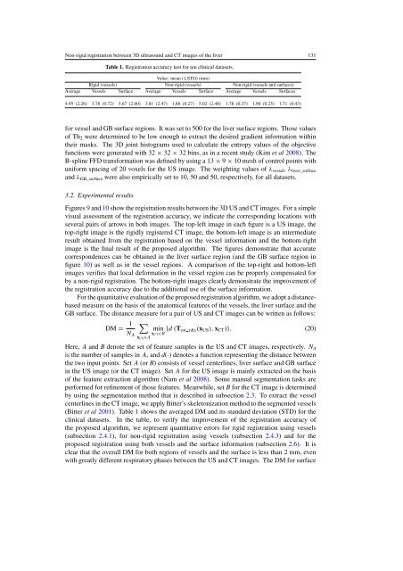3D B-mode US images were also acquired using aMedison Accuvix V10 ultrasound scanner equipped with a mechanical 3D US probe. Atypical image dimension is 200 × 124 × 148 in the Cartesian coordinates with an isotropicvoxel size of 1.82 mm 3 . For the experiment, we acquired 3D US images at the respiratoryphase of close-expiration with a breath-hold. This point is clearly distinct from the respiratoryphase in the CT images.To extract the gradient information, the value of Th 2 was empirically set to 10 in all of theUS images. Meanwhile, in the CT images, the value of Th 2 was set to 100, which is common
Non-rigid registration between 3D ultrasound and CT images of the liver 131Table 1. Registration accuracy test for ten clinical datasets.Value: mean (±STD) (mm)Rigid (vessels) Non-rigid (vessels) Non-rigid (vessels and surfaces)Average Vessels Surface Average Vessels Surface Average Vessels Surfaces4.95 (2.26) 3.78 (0.72) 5.67 (2.60) 3.81 (2.47) 1.88 (0.27) 5.02 (2.48) 1.78 (0.37) 1.90 (0.25) 1.71 (0.43)for vessel and GB surface regions. It was set to 500 for the liver surface regions. Those valuesof Th 2 were determined to be low enough to extract the desired gradient information withintheir masks. The 3D joint histograms used to calculate the entropy values of the objectivefunctions were generated with 32 × 32 × 32 bins, as in a recent study (Kim et al 2008). TheB-spline FFD transformation was defined by using a 13 × 9 × 10 mesh of control points withuniform spacing of 20 voxels for the US image. The weighting values of λ vessel , λ liver_surfaceand λ GB_surface were also empirically set to 10, 50 and 50, respectively, for all datasets.3.2. Experimental resultsFigures 9 and 10 show the registration results between the 3D US and CT images. For a simplevisual assessment of the registration accuracy, we indicate the corresponding locations withseveral pairs of arrows in both images. The top-left image in each figure is a US image, thetop-right image is the rigidly registered CT image, the bottom-left image is an intermediateresult obtained from the registration based on the vessel information and the bottom-rightimage is the final result of the proposed algorithm. The figures demonstrate that accuratecorrespondences can be obtained in the liver surface region (and the GB surface region infigure 10) as well as in the vessel regions. A comparison of the top-right and bottom-leftimages verifies that local deformation in the vessel region can be properly compensated forby a non-rigid registration. The bottom-right images clearly demonstrate the improvement ofthe registration accuracy due to the additional use of the surface information.For the quantitative evaluation of the proposed registration algorithm, we adopt a distancebasedmeasure on the basis of the anatomical features of the vessels, the liver surface and theGB surface. The distance measure for a pair of US and CT images can be written as follows:DM = 1 ∑minN {d (T est v&s(x US ), x CT )}. (20)A x CT ∈Bx US ∈AHere, A and B denote the set of feature samples in the US and CT images, respectively. N Ais the number of samples in A, and d(·) denotes a function representing the distance betweenthe two input points. Set A (or B) consists of vessel centerlines, liver surface and GB surfacein the US image (or the CT image). Set A for the US image is mainly extracted on the basisof the feature extraction algorithm (Nam et al 2008). Some manual segmentation tasks areperformed for refinement of those features. Meanwhile, set B for the CT image is determinedby using the segmentation method that is described in subsection 2.3. To extract the vesselcenterlines in the CT image, we apply Bitter’s skeletonization method to the segmented vessels(Bitter et al 2001). Table 1 shows the averaged DM and its standard deviation (STD) for theclinical datasets. In the table, to verify the improvement of the registration accuracy ofthe proposed algorithm, we represent quantitative errors for rigid registration using vessels(subsection 2.4.1), for non-rigid registration using vessels (subsection 2.4.3) and for theproposed registration using both vessels and the surface information (subsection 2.6). It isclear that the overall DM for both regions of vessels and the surface is less than 2 mm, evenwith greatly different respiratory phases between the US and CT images. The DM for surface
Page 1 and 2: IOP PUBLISHINGPhys. Med. Biol. 56 (
Page 3 and 4: Non-rigid registration between 3D u
Page 13: Non-rigid registration between 3D u
Page 21: Non-rigid registration between 3D u

Non-rigid registration between 3D ultrasound and CT ... - isl, ee, kaist

Create successful ePaper yourself

Delete template?

Save as template?