Hypothesis Testing (One-Sample Tests)
Hypothesis Testing (One-Sample Tests)
Hypothesis Testing (One-Sample Tests)
- No tags were found...

You also want an ePaper? Increase the reach of your titles
YUMPU automatically turns print PDFs into web optimized ePapers that Google loves.
<strong>Hypothesis</strong> <strong>Testing</strong><br />
(<strong>One</strong>-<strong>Sample</strong> <strong>Tests</strong>)
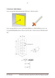
What is a <strong>Hypothesis</strong>?<br />
•A hypothesis is a<br />
claim (assumption)<br />
about the population<br />
parameter<br />
–Examples of parameters<br />
are population mean<br />
or proportion<br />
–The parameter must<br />
be identified before<br />
analysis<br />
I claim the mean GPA of<br />
this class is 3.5!<br />
µ =<br />
©1984-1994 T/Maker Co.
The Null <strong>Hypothesis</strong>, H 0<br />
•States the assumption (numerical) to be<br />
tested<br />
–e.g.: The average number of TV sets in U.S.<br />
Homes is at least three ( )<br />
H : µ ≥ 3<br />
0<br />
•Is always about a population parameter<br />
( H : µ ≥ 3 ), not about a sample statistic<br />
0<br />
( H : X ≥ 3 )<br />
0
The Null <strong>Hypothesis</strong>, H 0<br />
•Begins with the assumption that the null<br />
hypothesis is true<br />
–Similar to the notion of innocent until<br />
proven guilty<br />
•Always contains the “=” sign<br />
•May or may not be rejected<br />
(continued)
The Alternative <strong>Hypothesis</strong>, H 1<br />
•Is the opposite of the null hypothesis<br />
–e.g.: The average number of TV sets in<br />
U.S. homes is less than 3 ( )<br />
H<br />
1<br />
: µ < 3<br />
•Never contains the “=” sign<br />
•May or may not be accepted<br />
•Is generally the hypothesis that is<br />
believed (or needed to be proven) to<br />
be true by the researcher
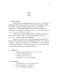
<strong>Hypothesis</strong> <strong>Testing</strong> Process<br />
Assume the<br />
population<br />
mean age is 50.<br />
( )<br />
0 : 50<br />
Identify the Population<br />
H µ =<br />
( )<br />
X<br />
= 20 likely if =50<br />
Is µ ?<br />
No, not likely!<br />
Take a <strong>Sample</strong><br />
REJECT<br />
Null <strong>Hypothesis</strong><br />
X = 20
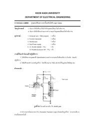
Reason for Rejecting H 0<br />
Sampling Distribution of<br />
X<br />
It is unlikely that<br />
we would get a<br />
sample mean of<br />
this value ...<br />
... Therefore,<br />
we reject the<br />
null hypothesis<br />
that m = 50.<br />
... if in fact this were<br />
the population mean.<br />
20<br />
m<br />
= 50<br />
If H 0 is true<br />
X
Level of Significance,<br />
α<br />
•Defines unlikely values of sample statistic<br />
if null hypothesis is true<br />
–Called rejection region of the sampling<br />
distribution<br />
•Is designated by<br />
α<br />
–Typical values are .01, .05, .10<br />
, (level of significance)<br />
•Is selected by the researcher at the<br />
beginning<br />
•Provides the critical value(s) of the test
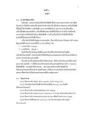
Level of Significance<br />
and the Rejection Region<br />
H 0 : m ‡ 3<br />
H 1 : m < 3<br />
a<br />
Critical<br />
Value(s)<br />
H 0 : m £ 3<br />
H 1 : m > 3<br />
H 0 : m = 3<br />
H 1 : m „ 3<br />
Rejection<br />
Regions<br />
0<br />
0<br />
0<br />
a<br />
a/2
Errors in Making Decisions<br />
•Type I Error<br />
–Rejects a true null hypothesis<br />
–Has serious consequences<br />
The probability of Type I Error is<br />
•Called level of significance<br />
•Set by researcher<br />
•Type II Error<br />
–Fails to reject a false null hypothesis<br />
–The probability of Type II Error is β<br />
–The power of the test is 1−<br />
β<br />
( )<br />
α
Errors in Making Decisions<br />
•Probability of not making Type I Error<br />
–<br />
1−α<br />
( )<br />
–Called the confidence coefficient<br />
(continued)
Result Probabilities<br />
The Truth<br />
H 0 : Innocent<br />
Jury Trial <strong>Hypothesis</strong> Test<br />
The Truth<br />
Verdict Innocent Guilty Decision H 0 True H 0 False<br />
Innocent Correct Error<br />
Guilty Error Correct<br />
Do Not<br />
Reject<br />
H 0<br />
Reject<br />
H 0<br />
1 - a<br />
Type I<br />
Error<br />
(a )<br />
Type II<br />
Error (b )<br />
Power<br />
(1 - b )
How to Choose between<br />
Type I and Type II Errors<br />
•Choice depends on the cost of the errors<br />
•Choose smaller Type I Error when the<br />
cost of rejecting the maintained<br />
hypothesis is high<br />
–A criminal trial: convicting an innocent person<br />
•Choose larger Type I Error when you<br />
have an interest in changing the status<br />
–A decision in a startup company about a new<br />
piece of software
Critical Values<br />
Approach to <strong>Testing</strong><br />
•Convert sample statistic (e.g.: X ) to test<br />
statistic (e.g.: Z, t or F –statistic)<br />
•Obtain critical value(s) for a specified<br />
from a table or computer<br />
–If the test statistic falls in the critical region,<br />
reject H 0<br />
–Otherwise do not reject H 0<br />
α
p-Value Approach to <strong>Testing</strong><br />
•Convert <strong>Sample</strong> Statistic (e.g. ) to Test<br />
Statistic (e.g. Z, t or F –statistic)<br />
•Obtain the p-value from a table or computer<br />
–p-value: Probability of obtaining a test statistic<br />
more extreme ( or ) than the observed<br />
sample value given H 0 is true<br />
X<br />
≤ ≥<br />
α<br />
–If p-value , do not reject H 0<br />
–If p-value ≤ , reject H 0<br />
–Called observed level of significance<br />
–Smallest value of α that an H 0 can be rejected<br />
•Compare the p-value with<br />
≥ α<br />
α
General Steps in<br />
<strong>Hypothesis</strong> <strong>Testing</strong><br />
e.g.: Test the assumption that the true mean<br />
number of of TV sets in U.S. homes is at least<br />
three ( σ Known)<br />
1. State the H 0<br />
2. State the H 1<br />
3. Choose<br />
α<br />
4. Choose n<br />
5. Choose Test<br />
H<br />
H<br />
α<br />
n<br />
Z<br />
0<br />
1<br />
: µ ≥ 3<br />
: µ < 3<br />
=.05<br />
= 100<br />
test
General Steps in<br />
<strong>Hypothesis</strong> <strong>Testing</strong><br />
6. Set up critical value(s)<br />
Reject H 0<br />
a<br />
(continued)<br />
7. Collect data<br />
8. Compute test statistic<br />
and p-value<br />
9. Make statistical decision<br />
-1.645<br />
100 households surveyed<br />
Computed test stat =-2,<br />
p-value = .0228<br />
Reject null hypothesis<br />
Z<br />
10. Express conclusion<br />
The true mean number of TV<br />
sets is less than 3
<strong>One</strong>-tail Z Test for Mean<br />
( σ Known)<br />
•Assumptions<br />
–Population is normally distributed<br />
–If not normal, requires large samples<br />
–Null hypothesis has or sign only<br />
• Z test statistic<br />
–<br />
Z<br />
X<br />
≤<br />
≥<br />
X − µ X − µ<br />
=<br />
X<br />
=<br />
σ σ / n
Rejection Region<br />
H 0 : m ‡ m 0<br />
H 1 : m < m 0<br />
H 0 : m £ m 0<br />
H 1 : m > m 0<br />
Reject H 0<br />
α<br />
Reject H 0<br />
α<br />
0<br />
Z Must Be Significantly<br />
Below 0 to reject H 0<br />
Z<br />
0<br />
Small values of Z don’t<br />
contradict H 0<br />
Don’t Reject H 0 !<br />
Z
Example: <strong>One</strong> Tail Test<br />
Q. Does an average box<br />
of cereal contain more<br />
than 368 grams of<br />
cereal? A random<br />
sample of 25 boxes<br />
showed X = 372.5.<br />
The company has<br />
specified s to be 15<br />
grams. Test at the a =<br />
0.05 level.<br />
368 gm.<br />
H 0 : m £ 368<br />
H 1 : m > 368
Finding Critical Value: <strong>One</strong> Tail<br />
What is Z given α = 0.05?<br />
Standardized Cumulative<br />
Normal Distribution Table<br />
(Portion)<br />
σ =<br />
Z<br />
1<br />
.95<br />
α = .05<br />
Z .04 .05 .06<br />
1.6 .9495 .9505 .9515<br />
1.7 .9591 .9599 .9608<br />
Critical Value<br />
= 1.645<br />
0 1.645<br />
Z<br />
1.8 .9671 .9678 .9686<br />
1.9 .9738 .9744 .9750
Example Solution: <strong>One</strong> Tail Test<br />
H 0 : m £ 368<br />
H 1 : m > 368<br />
a = 0.5<br />
n = 25<br />
Critical Value: 1.645<br />
Reject<br />
.05<br />
0 1.645<br />
1.50<br />
Z<br />
Test Statistic:<br />
X −µ<br />
Z = = 1.50<br />
σ<br />
n<br />
Decision:<br />
Do Not Reject at α = .05<br />
Conclusion:<br />
No evidence that true<br />
mean is more than 368
p -Value Solution<br />
p-Value is P(Z ‡ 1.50) = 0.0668<br />
Use the<br />
alternative<br />
hypothesis<br />
to find the<br />
direction of<br />
the rejection<br />
region.<br />
From Z Table:<br />
Lookup 1.50 to<br />
Obtain .9332<br />
0 1.50<br />
P-Value =.0668<br />
Z<br />
1.0000<br />
- .9332<br />
.0668<br />
Z Value of <strong>Sample</strong><br />
Statistic
p -Value Solution<br />
(p-Value = 0.0668) ‡ (a = 0.05)<br />
Do Not Reject.<br />
(continued)<br />
p Value = 0.0668<br />
Reject<br />
a = 0.05<br />
0<br />
1.645<br />
1.50<br />
Test Statistic 1.50 is in the Do Not Reject Region<br />
Z
Example: Two-Tail Test<br />
Q. Does an average<br />
box of cereal<br />
contain 368 grams<br />
of cereal? A<br />
random sample of<br />
25 boxes showed<br />
X = 372.5. The<br />
company has<br />
specified s to be 15<br />
grams. Test at the<br />
a = 0.05 level.<br />
368 gm.<br />
H 0 : m = 368<br />
H 1 : m „ 368
Example Solution: Two-Tail Test<br />
H 0 : m = 368<br />
H 1 : m „ 368<br />
a= 0.05<br />
n = 25<br />
Critical Value: ±1.96<br />
.025<br />
-1.96<br />
0 1.96<br />
1.50<br />
Reject<br />
.025<br />
Z<br />
Z<br />
Test Statistic:<br />
X −µ<br />
372.5−368 = = = 1.50<br />
σ 15<br />
n 25<br />
Decision:<br />
Do Not Reject at α = .05<br />
Conclusion:<br />
No Evidence that True<br />
Mean is Not 368
p-Value Solution<br />
(p Value = 0.1336) ‡ (a = 0.05)<br />
Do Not Reject.<br />
p Value = 2 x 0.0668<br />
Reject<br />
Reject<br />
a = 0.05<br />
0 1.50<br />
Z<br />
1.96<br />
Test Statistic 1.50 is in the Do Not Reject Region
Connection to<br />
Confidence Intervals<br />
For X = 372.5, σ = 15 and n=<br />
25,<br />
the 95% confidence interval is:<br />
372.5− 1.96 15/ 25≤µ<br />
≤ 372.5+<br />
1.96 15/ 25<br />
( ) ( )<br />
or<br />
366.62≤µ<br />
≤378.38<br />
If this interval contains the hypothesized mean (368),<br />
we do not reject the null hypothesis.<br />
It does. Do not reject.
t -Test:<br />
σ<br />
Unknown<br />
•Assumption<br />
–Population is normally distributed<br />
–If not normal, requires a large sample<br />
• T -test statistic with n-1 degrees of<br />
freedom<br />
–<br />
t<br />
=<br />
X − µ<br />
S/<br />
n
Example: <strong>One</strong>-Tail t -Test<br />
Does an average box of<br />
cereal contain more than<br />
368 grams of cereal? A<br />
random sample of 36<br />
boxes showed X = 372.5,<br />
and s = 15. Test at the a =<br />
0.01 level.<br />
s<br />
is not given<br />
368 gm.<br />
H 0 : m £ 368<br />
H 1 : m > 368
Example Solution: <strong>One</strong>-Tail<br />
H 0 : m £ 368<br />
H 1 : m > 368<br />
a = 0.01<br />
n = 36, df = 35<br />
Critical Value: 2.4377<br />
Reject<br />
0 2.4377<br />
1.80<br />
.01<br />
t 35<br />
t<br />
Test Statistic:<br />
X −µ<br />
372.5−368 = = = 1.80<br />
S 15<br />
n 36<br />
Decision:<br />
Do Not Reject at a = .01<br />
Conclusion:<br />
No evidence that true<br />
mean is more than 368
p -Value Solution<br />
(p Value is between .025 and .05) ‡ (a = 0.01).<br />
Do Not Reject.<br />
p Value = [.025, .05]<br />
Reject<br />
a = 0.01<br />
0 1.80<br />
t 35<br />
2.4377<br />
Test Statistic 1.80 is in the Do Not Reject Region