Journal

Journal
A LARSA Publication May 2010
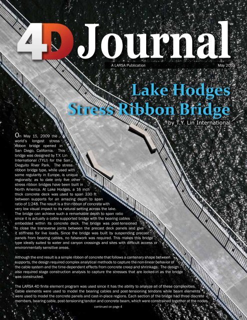
Lake Hodges
Stress Ribbon Bridge
by T.Y. Lin International
On May 15, 2009 the
world’s longest stress
ribbon bridge opened in
San Diego, California. This
bridge was designed by T.Y. Lin
International (TYLI) for the San
Dieguito River Park. The stress
ribbon bridge type, while used with
some regularity in Europe, is unique
regionally; as to date only five other
stress ribbon bridges have been built in
North America. At Lake Hodges, a 16 inch
thick concrete deck was used to span 330 ft
between supports for an amazing depth to span
ratio of 1:248. The result is a thin ribbon of concrete with
very low visual impact to its natural setting across the lake.
The bridge can achieve such a remarkable depth to span ratio
since it is actually a cable supported bridge with the bearing cables
embedded within its concrete deck. The bridge was post-tensioned
to close the transverse joints between the precast deck panels and give
it stiffness for live loads. Since the bridge was built by suspending precast
panels from bearing cables, no falsework was required. This makes this bridge
type ideally suited to water and canyon crossings and sites with difficult access or
environmentally sensitive areas.
Although the end result is a simple ribbon of concrete that follows a cantenary shape between
supports, the design required complex analytical methods to capture the non-linear behavior of
the cable system and the time-dependent effects from concrete creep and shrinkage. The design
also required stage construction analysis to capture the stresses that are locked-in as the bridge
was constructed.
The LARSA 4D finite element program was used since it has the ability to analyze all of these complexities.
Cable elements were used to model the bearing cables and post-tensioning tendons while beam elements
were used to model the concrete panels and cast-in-place regions. Each section of the bridge had three discrete
members, bearing cable, post-tensioning tendon and concrete beam, which were constrained together at the nodes.
continued on page 4

What’s Happening?
Latest News from LARSA, Inc.
by Joshua Tauberer
Director of Software Architecture
We have been hard at work as always improving our software
and responding to our clients’ needs. Here are some recent
developments.
Documentation
Six new manuals have been finished. Three are training
manuals, helping you get up to speed on modeling basic to
advanced bridges with LARSA 4D. Topics covered include 3D
straight and curved bridges, post-tensioning, nonprismatic
variation, Staged Construction Analysis, and live load using
influence lines and surfaces. They are:
You can find the manuals on our website, www.LARSA4D.
com. Click Support > Client Support Center > Product
Documentation.
Website
You never get a second chance to make a first impression, so
we took a hard look at our website www.LARSA4D.com and
decided it was time for a refresh. Besides making it more surferfriendly,
you can find on the website our interactive project
portfolio, back issues of the 4D Journal, and our brochures.
• LARSA 4D Introductory Training Manual
• LARSA 4D Basic Training Manual for Bridge Projects
• LARSA 4D Advanced Training Manual for Bridge Projects
There are also new manuals for LARSA Section Composer,
which doubles as a tutorial, for the LARSA 4D Steel Plate
Girder Design Module for AASHTO LRFD, and for LARSA 4D’s
Cable Tension Optimization Tools.
Visit Us
We'll be at the following upcoming conferences:
PCI/FIB Annual Convention and Bridge Conference
May 29 - June 2, 2010
Gaylord National Resort
Washington, D.C.
International Bridge Conference
June 6-9, 2010
David L. Lawrence Convention Center
Pittsburgh, PA
US National & Canadian Conference on Earthquake Engineering
July 25-29, 2010
Westin Harbor Castle Hotel
Toronto, Canada
ASBI Conference 2010
October 11-12, 2010
Vancouver, Canada
In the next issue of LAR-
SA’s 4D Journal:
Arbour Stone Bridge
continued on page 3
Up Next
A 120 meter twin steel
arch pedestrian bridge
built in The City of Calgary,
Alberta, Canada.
The consulting engineers
of Infinity Group, Ltd. of North Vancouver talk about
the project and LARSA 4D’s role in its creation.
Front Cover: Lake Hodges Stress Ribbon Bridge, San Diego, California courtesy of T.Y.Lin International
LARSA, Inc.
105 Maxess Road
Melville | New York | 11747
1-212-736-4326
www.LARSA4D.com
info@LARSA4D.com
LARSA 4D is analysis and design software for bridges, buildings, and other
structures, developed by LARSA, Inc. in New York, USA.
This journal is distributed as a courtesy to our clients and corporate friends.
We welcome feedback and suggestions for future stories to info@LARSA4D.com.
•LARSA’s 4D Journal • May 2010•Page 2

Features On Demand
Our team is well known for providing timely and useful
technical support, webinars, and on-site training. Our newest
support system is called “Features On Demand.” This allows
us to provide new features directly to waiting clients without
having to go through our normal software release cycle and
without the user having to uninstall and reinstall an updated
version of LARSA 4D (which can be inconvenient in corporate
offices). New features that we have been able to provide within
hours include automatic generation of bridge path coordinate
systems based on existing model geometry and computing the
length of patch loading in influence line analysis.
As the lean, mean, structure-solving machine, we always are
on the look-out for new ways to deliver on our promise for
unparalleled support services. “LARSA Live” is another new
tool in our arsenal for rapidly providing new custom-build tools
to our clients. LARSA Live allows users to run LARSA 4D off the
Internet without having to install it. This means users can run
an old and new version of LARSA 4D at the same time, and the
new version can be tested without requiring IT’s help to install
the program.
We’re Going Global
The software will soon be available in a select few languages
besides English. Our British clients have told us they can’t
understand our software’s New York drawl.
The Shell Element
It’s a common misconception that Indiana Jones was searching
for the Holy Grail. In fact, he was looking for the Unified Shell
Element, an advanced element formulation that will allow
users to combine separate plate and membrane models into a
single shell element.
Cable Reincarnation
What does reincarnation have to do with nonlinear analysis?
The cable element’s “rebirth” capability is when it goes in and
out of an analysis depending on whether it is under tension.
When the cable goes into compression, it is taken out of the
analysis because the cable has no compressive strength.
This can make nonlinear convergence more difficult, so we
LARSA 4D and Section Composer are being updated for composite
construction.
are adding a new option: cable compressive strength. When
this option is used, cables in compression will retain a small
fraction of their tensile strength.
Composite Sections (Almost!)
In software development it is notoriously difficult to estimate
how long it will take to deliver on a promise. More than three
years ago we began work on composite section construction.
This major update to the LARSA 4D analysis engine would
allow member cross-sections to be built up over time in the
Staged Construction Analysis. A girder might be placed first
with a deck (modeled in the cross-section) cast later on.
Though the parts are combined into a single line element,
they have different time-dependent effects such as creep. This
update also includes nonlinear thermal gradients. We began
previewing this update on a limited basis in 2010 and expect a
public preview later this year.•
After adding a “thick plate” element formulation, we
added drilling degrees of freedom to “membrane element”
formulation. Drilling degrees of freedom provide for more
realistic modeling when the shell is subject to a torque about
its normal axis.
We have also added shell element end offsets, much like
member end offsets, which is useful for creating rigid
connections between a girder and a deck. Twelve end offset
values (x, y, z for each node) can be entered for each plate.
Cable Compressive Strength is a new option for nonlinear analysis types to
make convergence easier.
•LARSA’s 4D Journal • May 2010•Page 3

Lake Hodges-Stress Ribbon Bridge
continued from page 1
Restrained nodes were sufficient to model the fixed north
abutment. However, the four pile shafts at the south abutment
were individually discretized in the model to account for their
non-linear behaviour of the soil.
Fig. 1 – Rendering of LARSA 4D Model
Thirdly, constructed of a continuous ribbon of prestressed
concrete, using common materials and construction methods,
the bridge would be economical to construct, extremely durable
and essentially maintenance free. And finally, the stress ribbon
design would result in a beautiful and unique pedestrian
bridge that would be a landmark for the San Dieguito River
Park and the region.
The firm Safdie Rabines Architects (SRA) was brought on
board to help with aesthetic details. SRA was instrumental in
the architectural shaping of the bridge. Jiri Strasky, who is well
known as a pioneer of the stress ribbon bridge type, was hired
to provide input on the conceptual design and to perform the
independent check of the bridge.
Aesthetics played a major role in the River Park’s decision to
go with the stress ribbon bridge type. Ricardo Rabines of SRA
developed some of the early sketches of the bridge and felt that
aesthetically the stress ribbon bridge was ideal for this setting
across Lake Hodges, since it blends harmoniously into the
surroundings in both wet and dry conditions. His description
for the stress ribbon bridge is one of “floating” over the water,
or “nesting” above the dry lakebed. See Fig. 2 and 3.
Architectural and Structural Solution
TYLI studied several bridge types during the type selection
process. Other structure types that were considered included:
reinforced concrete slab, precast concrete girders, castin-place
prestressed concrete box girder, timber glue-lam
girders, prefabricated steel trusses as well as suspension
and cable stayed alternatives. The TYLI led team and the
River Park worked together to select a bridge type that would
be economically feasible to construct and easy to maintain,
would compliment the site and most importantly would be
compatible with the River Park’s mission:
• To preserve and restore land within the Focused Planning Area of
the San Dieguito River Park as a regional open space greenway
and park system that protects the natural waterways and the
natural and cultural resources and sensitive lands and provides
compatible recreational opportunities, including water related
uses, that do not damage sensitive lands.
• To provide a continuous and coordinated system of preserved
lands with a connecting corridor of walking, equestrian, and
bicycle trails, encompassing the San Dieguito River Valley from
the ocean to the river’s source.
In the end, the stress ribbon bridge type prevailed for several
reasons. Firstly, this bridge type could be built with the 330 ft
spans required to limit the number of permanent supports within
the lake to two, and this could be accomplished with minimal
visual impact to the natural habitat since the deck would be
only 16 inches thick. Secondly, since the superstructure would
be built of precast panels suspended from bearing cables,
there would be no need for falsework, which would further
reduce impacts to the environmentally sensitive habitat and
also eliminate the expense of constructing falsework over a
major waterway.
•LARSA 4D’s Journal • May 2010•Page 4
Stage Construction Model
A stage construction analysis was conducted where the bridge
was “constructed” step-by-step within the computer model.
First the substructure elements were constructed, then the
bearing cables were installed, the weight from the precast
panels and cast-in-place concrete was applied, the concrete
stiffness was activated, then the post tensioning force was
applied and so forth. This stage construction analysis was
necessary to capture the stresses that were locked into
each component - bearing cable, concrete ribbon, and posttensioning
tendon - as the bridge was constructed. The stage
construction analysis also allowed the time dependent effects
of creep and shrinkage to be analyzed.
Time Dependent Effects
The creep and shrinkage functions from the CEB-FIP 78 code
built into the LARSA 4D program were used. The casting day
of each member and other creep and shrinkage parameters
were input into the program. After the bridge was constructed
in the model, the design load combinations were applied.
Next, 50 years of creep and shrinkage were applied in steps
and the load combinations were analyzed again. In the end the
load combination that included dead load, added dead load,
live load and a drop in temperature of 35 degrees Fahrenheit,
all applied after 50 years of creep and shrinkage, controlled
the design.
Thermal Loading Combination
The behavior of the continuous concrete ribbon was such that
each load in the controlling load combination tended to pull
on the ribbon and when combined resulted in tension in the
concrete. Initially the post tensioning put the concrete ribbon
into compression, but this compression was reduced by the

added dead load.
Creep and shrinkage
had the effect of
causing the bridge
to shorten, move
upward, and further
reduced the amount
of pre-compression.
The applied live
load and a drop in
temperature of 35
degrees Fahrenheit
further acted to put
the concrete ribbon
into tension. The
design intent was to
keep the concrete
ribbon from going
into tension under permanent loads and to keep tension to a
reasonable level under the extreme case of full live load and
thermal loading.
The controlling load combination for the superstructure was as
follows: 1.0 D + 1.0 L + 1.0 PS + 1.0 T + 1.0 C&S
Where D is dead load, L is live load, PS is prestress, T is thermal
loading and C&S is creep and shrinkage. The allowable stress
in this condition was 125% of the basic allowable stress.
Allowable extreme fiber tension stress in the concrete under
this combination was:
f t
= 1.25 x 3√ f’c [psi]
For the superstructure concrete, which has a specified nominal
compression strength of f’c = 6,000 psi, the allowable tension
stress is 290 psi.
Since the probability of the bridge being simultaneously
subjected to maximum live load and maximum thermal loading
is very low, a reduction of 25% to one or the other was allowed.
The result was that a post-tensioning force of 4,600 kips was
required to meet the above design criterion.
Capacity for Overload
One of the interesting characteristics of the stress ribbon
bridge type is its remarkable capacity for overload. LARSA
4D was used to investigate this. In this analytical study,
the pedestrian live loading was incrementally increased.
At a four-fold increase in the live loading, the study showed
the bridge could easily carry the increased load with only a
nominal stress increase to the bearing and post-tensioning
cables. The extra load carrying capacity instead comes from
the change in the cable geometry. Increased cable sag results
in the corresponding increase in the vertical load carrying
component of the cables.
Dynamic Analysis
A dynamic analysis was required to assess the performance
of the bridge to live load vibrations, heavy winds, and seismic
•LARSA 4D’s Journal • May 2010•Page 5
actions.
Since the stiffness of
the bridge changes
with applied loading,
a “stressed Eigenvalue”
analysis
was required to
determine the
natural frequencies
and mode shapes.
This is a special
type of Eigen-value
analysis in which
the stiffness matrix
includes the static
loads and the
deformed geometry
of the structure. Within the stage construction model, the
bridge was constructed, post-tensioning was applied, the
superimposed dead load was applied, then the Eigen-values
were determined. It was important to determined the Eigenvalues
at this state of stress in the bridge to get the correct
stiffness. The first three mode shapes are shown in Fig. 4.
Fig. 2 – Rendering of completed bridge, looking west, lake filled with water
Fig. 3 – Rendering of completed bridge, looking southeast, dry lake condition
The results of the analysis showed that modes 1 and 2 each
have less than 0.02 percent mass participation, while mode 3
captures about 20 percent mass participation. Thus, mode 3
is the vertical mode used to investigate the bridge’s sensitivity
to excitation from pedestrians.
Live Load Vibrations
The vibrations from pedestrian loading on the bridge were
evaluated based on simplified approaches from the British
and Ontario bridge codes. Both codes specify a simple design
procedure that determines the vertical acceleration resulting
from the passage of one pedestrian walking with a pace
equal to the fundamental natural frequency of the bridge. The
procedure is for a bridge excitation by one pedestrian and no
allowance is made for multiple random arrivals of pedestrians.
For footbridges up to three spans, the estimated vertical
acceleration is:
a = 4π 2 f 1
2
yKψ [ft/s 2 ]
Where f 1
= fundamental natural frequency of the bridge [Hz]
y = static deflection at mid-span for a force of 160 lbs [ft]
K = configuration factor
Ψ = dynamic response factor
The fundamental frequency and static deflection at midspan
were determined from the finite element model. The
stressed Eigen-value analysis resulted in fundamental vertical
frequency of f 1
= 0.74 Hz. The static deflection at mid-span
for a 160 lb force (static weight of one pedestrian) was y =
0.0014 ft.
The configuration factor, K, is based on the number of spans
and is 1.0 for a single span, 0.7 for a two-span, and between
continued on page 6

Lake Hodges-Stress Ribbon Bridge
continued from page 5
properties of the bridge were required. Wind tunnel tests on
a 1/10 scale model of the bridge section were performed to
determine the aerodynamic load characteristics on the bridge
deck, Fig. 5.
a) Mode 1 – 0.43 Hz
b) Mode 2 – 0.45 Hz
c) Mode 3 – 0.74 Hz
Fig. 4 – Mode Shapes from the Stressed Eigen-value Analysis
0.6 and 0.9 for a three-span bridge. For the three-span Lake
Hodges Bridge, the upper limit of K= 0.9 was conservatively
used.
Fig. 5 – Wind tunnel testing of a 1/10 scale model
The aerodynamic turbulence field was described by a series of
horizontal and vertical wind speed time histories at 30 nodes
along the length of the bridge, Fig. 6.
The dynamic response factor, Ψ, is given in graphical form as
a function of the span length and damping ratio. For the Lake
Hodges bridge, a damping ratio of 0.010 was used, which is
considered to be appropriate for a prestressed concrete
footbridge. Using this damping ratio with a 330 ft span resulted
in a dynamic response factor of Ψ = 39. Using these values in
Equation 4 gives a vertical acceleration of a = 0.33 ft/s 2 .
This vertical acceleration must be compared to the allowable
limits specified by the codes. For fundamental natural
frequencies, f1 less than 5 Hz, the British code gives a
vibrational acceleration serviceability limit of:
a max
= 0.8 f 1
0.5
[ft/s 2 ]
The Ontario code gives a more conservative serviceability limit
of:
a max
= 0.8 f 1
0.78
[ft/s 2 ]
For f1 = 0.74 Hz, the allowable limits are 1.4 ft/s 2 and 0.65
ft/s 2 , respectively for the British and Ontario codes. The
calculated acceleration for the Lake Hodges Bridge, at 0.33
ft/s 2 , is well below these allowable limits.
Furthermore, the fundamental vertical frequency of the
Lake Hodges Bridge at 0.74 Hz is well outside of the natural
frequencies of footfall, which are typically in the range of 1.65
to 2.35 Hz for walking pedestrians or up to 3.5 Hz for running
pedestrians. Thus, the analysis determined that live load
vibrations would not be a problem for the Lake Hodges Bridge.
Wind Analysis
To verify that the bridge would be stable under heavy winds,
a special wind analysis was performed by West Wind Labs
to determine the bridge buffeting response. To do this, the
aerodynamic load characteristics of the bridge, a description
of the aerodynamic turbulence, and the mechanical dynamic
•LARSA 4D’s Journal • May 2010•Page 6
Fig. 6 – Numerical model of the bridge
The dynamic properties, dominant mode shapes and
frequencies of the bridge, were determined from the LARSA
4D finite element model.
A numerical simulation procedure was then used. Wind speed
time histories at 30 nodes along the bridge deck and 20
modes of vibration were included in the analysis. Numerical
simulations for a duration of 5 minutes, with a typical step
size of 0.02 seconds, were generated. Bridge stability was
evaluated by comparing the modal responses at the end of
the simulation to the corresponding modal responses at the
beginning of the simulations. Statistics of the steady state
modal responses were used to generate a buffeting response.
For horizontal winds from the east and west (perpendicular to
the axis of the bridge), a numerical simulation was performed
for mean wind speeds (here assumed to be a ten minute
averaged wind speed) of 67, 71, 76, 80, 85, 89 and 94 mph.

The numerical simulations were performed in smooth flow.
At the beginning of each simulation, all modes of vibration
began with a modal displacement of unity. Each mode was
released in the specified wind, and all were allowed to vibrate
freely and simultaneously, allowing for any cross coupling
should there be an aerodynamic tendency to do so. Dynamic
flutter instabilities (single-degree-of-freedom and coupled
multi-degree-of-freedom flutter instabilities) were then
identified by the ratios of the modal standard deviations at
the end of the simulations to the corresponding initial modal
standard deviations. If a modal ratio was greater than unity,
then that mode was diverging and the bridge was dynamically
unstable.
The results showed that the bridge would remain stable up
to a wind speed of 86 mph, which exceeded the maximum
expected wind speed at the site.
Seismic Analysis
To evaluate the seismic demands on the bridge, a response
spectrum analysis was performed using the mode shapes,
which were derived from the stressed Eigen-value analysis.
The seismic loading for the site was controlled by a moment
magnitude 7.0 event on the Rose Canyon fault, located
approximately 14 miles to the southwest. The 1996 California
Seismic Hazard Map was used to estimate a peak bedrock
acceleration of 0.3g for the site corresponding to the maximum
credible earthquake. The response spectrum analysis
showed very small seismic demands. At the tops of the piers,
transverse demands were less than 1.0 inch, and longitudinal
demands were less than 0.6 inches. Displacement demands
of this magnitude indicated that the bridge will remain elastic
under seismic loading. The robust seismic performance of this
bridge is intuitive as the mass of the thin superstructure is
small and lateral movement is restrained by a very large cable
force. Thus, seismic demands did not control any aspect of the
design, which is highly unusual for a bridge in California.
Partial Prestress Design
Although the majority of the superstructure was designed as
fully prestressed concrete, using gross section properties to
calculate the stresses within the 16 inch thick panels, near
the supports this was not feasible due to excessive positive
moment demands. The high moment demands are a result of
the stress ribbon construction method. When a stress ribbon
bridge is post-tensioned, the ends of each span rotate as the
concrete ribbon is lifted upward by the prestress force. This
results in positive moment demands at the ends of each span
that are an order of magnitude greater than the negative
moment demands along the rest of the structure. Fig. 7 shows
the bending moment demands after post-tensioning and
permanent loads have been applied. The negative moment
demands are relatively constant with a maximum of -228 kipft,
The positive moment demands spike near the supports
and reach a maximum of 3,370 kip-ft which is 15 times the
negative moment demand.
prestress design method was used. Partial prestress theory
accounts for cracking of the prestressed concrete section
under service loads. The design methodology is similar to
Fig. 7 – Bending moment under permanent loading, Mneg = -228 kip-ft,
Mpos = 3,370 kip-ft
working stress design for conventionally reinforced concrete
sections. However, the effect of prestressing must be
accounted for. The concrete section is allowed to crack and the
tensile stresses are resisted by the mild-steel reinforcing bars.
Bending moment demands were calculated from the finite
element model and a special MathCAD program was written
to calculate the resulting stresses in the concrete and steel for
each section.
Under the temporary condition before prestress losses, the
allowable extreme fiber compression stress in the concrete
is limited to 0.55f’ci. After prestress losses, the allowable
stresses in the concrete are 0.40f’c under permanent loads
and 0.60f’c under permanent plus live loads. The allowable
stress in the mild steel is 0.40fy. The allowable stress in the
prestressing steel is 0.72f’s. Allowable stresses are increased
by 25% when temperature or wind is used in the service load
combination.
The solution for the Lake Hodges Bridge was to haunch the
ends of each span over a 20 ft length from a typical thickness
of 16 inches to 36 inches at the face of support. The mildsteel
(Grade 60 ksi) reinforcing required at the 36 inch thick
section at the face of support consisted of 28 - #10 bars
along the bottom edge for a tension steel area of 35.6 in 2 and
a reinforcing ratio of 0.60%. The 16 inch thick section 20 ft
from face of support required 17 - #10 and 12 - #6 bars for a
tension steel area of 26.5 in 2 and a reinforcing ratio of 1.2%.
A unique structure type was used for the 302-meter-long
Lake Hodges Bicycle/Pedestrian Bridge. In North America,
the stress ribbon bridge type has only been used a handful
of times, and world-wide an example of this length has never
before been constructed. This special stress ribbon design
required specialized analysis procedures, which are typically
not necessary for standard bridges. The analyses showed
that the Lake Hodges Stress Ribbon Bridge will be safe for
dead and live loads and robust for overload, will perform
adequately under long-term creep and shrinkage loading,
will not be susceptible to live load vibrations, will be stable
under the maximum wind loading expected at the site, and will
resist loads imposed by the maximum credible earthquake.
Considerable effort went into the analysis and design of this
bridge. However, the extra effort has resulted in a world-class
bridge that will compliment its natural setting across Lake
Hodges and within the San Dieguito River Open Space Park
and will be a major asset to the people of San Diego County.•
To deal with these large positive bending moments, a partial
•LARSA 4D’s Journal • May 2010•Page 7

Live Load Analysis
with Influence Surfaces
by Joshua Tauberer
Director of Software Architecture
Live load codes impose some
of the most computationally
intensive requirements on
structural analysis. On a bridge
deck of a certain size, what
are the locations of the traffic
lanes and the vehicles on the
lanes that produce the greatest
moment somewhere on the
structure? Design codes add
on top of the variability in traffic
lane and vehicle locations the
additional variability of vehicle
type and length. One traffic lane
may be loaded with a special
permit truck and the remainder
with AASHTO LRFD HL-93s, each
with variable rear axle spacing.
Compared to the static analysis which in finite element
analysis has the closed-form solution D=K -1 P (the inverse of
the stiffness matrix multiplied by the load vector), live load
analysis is a much more intensive combinatorial problem.
LARSA 4D includes influence analysis using both influence lines
and influence surfaces. Influence lines are used in models in
which the deck surface is modeled as a part of the girder lineelement
cross-sections. Each influence line represents a single
traffic lane at a user-identified transverse location. The lines
may be put together into factored combinations using LARSA
4D’s linear result combinations and extreme effect groups
tools. Options include vehicle type (standard or user-defined),
variable axle spacing, variable vehicle spacing for multiple
vehicles, patch loading for UDL, and (in LARSA 4D version 7.5)
factors for centrifugal force effects for curved bridges. Also
supported is the span-by-span loading requirement of AASHTO
LFD. (A tutorial for influence lines can be found in the LARSA
4D Introductory Training Manual for Bridge Projects.)
Influence surfaces are a much more powerful and robust
method for live load analysis. With an influence surface
computed for the entire deck surface area, LARSA 4D can
automatically find the transverse locations of as many traffic
lanes as will fit on the surface. This saves the user the time
of choosing lane locations, modeling separate influence
lines, and forming factored combinations. With an influence
surface the separate lane effects are combined using supplied
multiple presence factors automatically. Additional options
for influence surfaces include traffic lane width, vehicle
margins, and UDL width within each traffic lane, and having
up to one lane with a different vehicle from the rest for local
permit loading. Influence lines and surfaces can be used with
curved and skewed bridges. (A tutorial for influence surfaces
Influence Surface Results Case Window
•LARSA’s 4D Journal • May 2010•Page 8
can be found in the LARSA 4D
Advanced Training Manual for
Bridge Projects.)
LARSA 4D has introduced new
tools for live load analysis in each
major update. Starting in version
7.5 of LARSA 4D, influence
analysis has been upgraded to
be significantly faster especially
for wide decks that fit three or
more traffic lanes. The analysis
also makes use of multi-core/
multi-CPU computers, spreading
the combinatorial investigation
across all available processors.
We have found a 2x speed
improvement on four processor
cores and a 4x speed improvement on eight processor cores,
on top of the speed improvements compared to influence
surface analysis in version 7.01 found even on single-core
computers. The new version also adds support for the spanby-span
requirement of AASHTO LFD to influence surfaces with
automatic lane positioning.
As with all development at LARSA, new capabilities are always
driven by feedback from our clients. We look forward to hearing
how we can continue to evolve LARSA 4D’s live load analysis to
meet all of our clients’ project requirements.
What’s New To Influence Surface Analysis in LARSA 4D Version
7.5
• Centrifugal force factors can be specified which automatically
adjusts vehicle wheel magnitudes. Multiple factors can be
specified to apply difference factors on different segments of
a single influence surface.
• Some codes require at most one lane of one vehicle type, with
the remaining lanes loaded with HL-93. This is now supported.
• AASHTO LFD point loading is now supported for influence
surfaces with multiple design lanes.
• Influence analysis is now multi-threaded on computers with
multiple processors or multiple cores.
• Influence surface coefficient grid spacing can be larger without
as much loss of accuracy because of better load positioning.
• Results are faster and more accurate when more than two
vehicles are placed on the surface because of an improved
vehicle position search procedure.
• Influence surface design lanes are now able to include UDL
without vehicle loading to allow more flexibility in creating load
combinations.•