PDFF Velocity Control: Extending PI

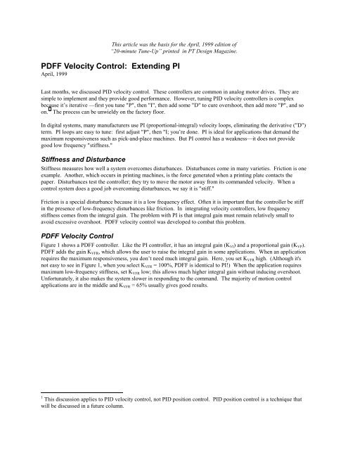
This article was the basis for the April, 1999 edition of
“20-minute Tune-Up” printed in PT Design Magazine.
PDFF Velocity Control: Extending PI
April, 1999
Last months, we discussed PID velocity control. These controllers are common in analog motor drives. They are
simple to implement and they provide good performance. However, tuning PID velocity controllers is complex
because it’s iterative —first you tune "P", then "I", then add some "D" to cure overshoot, then add more "P", and so
on. 1 The process can be unwieldy on the factory floor.
In digital systems, many manufacturers use PI (proportional-integral) velocity loops, eliminating the derivative ("D")
term. PI loops are easy to tune: first adjust "P", then "I; you’re done. PI is ideal for applications that demand the
maximum responsiveness such as pick-and-place machines. But PI control has a weakness—it does not provide
good low frequency "stiffness."
Stiffness and Disturbance
Stiffness measures how well a system overcomes disturbances. Disturbances come in many varieties. Friction is one
example. Another, which occurs in printing machines, is the force generated when a printing plate contacts the
paper. Disturbances test the controller; they try to move the motor away from its commanded velocity. When a
control system does a good job overcoming disturbances, we say it is "stiff."
Friction is a special disturbance because it is a low frequency effect. Often it is important that the controller be stiff
in the presence of low-frequency disturbances like friction. In integrating velocity controllers, low frequency
stiffness comes from the integral gain. The problem with PI is that integral gain must remain relatively small to
avoid excessive overshoot. PDFF velocity control was developed to combat this problem.
PDFF Velocity Control
Figure 1 shows a PDFF controller. Like the PI controller, it has an integral gain (KVI) and a proportional gain (KVP).
PDFF adds the gain KVFR, which allows the user to raise the integral gain in some applications. When an application
requires the maximum responsiveness, you don’t need much integral gain. Here, you set KVFR high. (Although it's
not easy to see in Figure 1, when you select KVFR = 100%, PDFF is identical to PI!) When the application requires
maximum low-frequency stiffness, set KVFR low; this allows much higher integral gain without inducing overshoot.
Unfortunately, it also makes the system slower in responding to the command. The majority of motion control
applications are in the middle and KVFR = 65% usually gives good results.
1
This discussion applies to PID velocity control, not PID position control. PID position control is a technique that
will be discussed in a future column.

Velocity
Command
+
Tuning PDFF
-
Estimate Velocity
KVFR
KVI∫ dt
+
+
-
Velocity
Feedback
Position Feedback
KVP
Current
Cmd.
Current
Loop
Actual
Current
Motor
Encoder/Resolver
Figure 1: Block diagram of PDFF-based velocity loop.
The following three-step procedure shows how to tune PDFF velocity control:
1. Tune KVP
Command a step velocity. Temporarily configure PDFF as a proportional-only controller by setting KVFR =
100% and KVI = 0. Raise KVP as high as possible without causing overshoot or oscillation.
2. Select KVFR for the application.
• Set KVFR to 100% for applications which require the greatest response
• Set KVFR to 65% for general applications
• Set KVFR to 0% for applications which require the greatest low-frequency stiffness
3. Raise KVI for 5% overshoot.
Figure 2 compares the command and the feedback for each of these steps for a PDFF controller. First KVP was
raised to just below the level causing overshoot (KVP=1.2). Then KVFR was set to 65%, assuming a general
application. Finally, KVI was raised for 5% overshoot (KVI =220). Use this same process for PI control, but skip
step 2—remember PI is just the special case of PDFF where KVFR = 100%. PI works well in applications where
low-frequency stiffness is not critical.
Step 1: KVFR =100, KVI = 0.
Raise KVP to max (Value = 1.2)
Step 2: Select KVFR for
application. (Value = 65%)
Figure 2: 3 Steps for tuning PDFF
Step 3: Raise KVI for 5%
overshoot. (Value = 220)

Practice tuning
The simulations above were run on a stand-alone simulation package called ModelQ. It is available at
www.ptdesign.com. After installation, click "Run" and at top left, and select the April model from the combo-box at
top center. Select the "Constants" tab and start adjusting KVP, KVI and KVFR. After you have entered a set of
constants with a good step response, run a Bode plot (press "GO" near center-bottom) and check the bandwidth. Try
tuning KVI with different values of KVFR. Notice that increasing KVFR causes overshoot which can be removed by
reducing KVI. Draw more Bode plots and watch the bandwidth go up as you increase KVFR. By the way, you can
also measure the responsiveness by watching the settling time to a step. As the bandwidth goes up, the settling time
goes down.
Application
Applications where a motor drives a worm gear often require maximum low-frequency stiffness. This is because
worm gear mechanisms usually have a lot of friction. Without a high integral gain, worm gear systems pull in to
position at the end of a move slowly. When people use PI controllers for worm-gear mechanisms, they sometimes
are not pleased with the long settling times the sometimes result. PDFF control can help this problem because
reducing KVFR=0 allows high integral gains, usually 8 - 10 times larger than the integral gain of a PI controller.