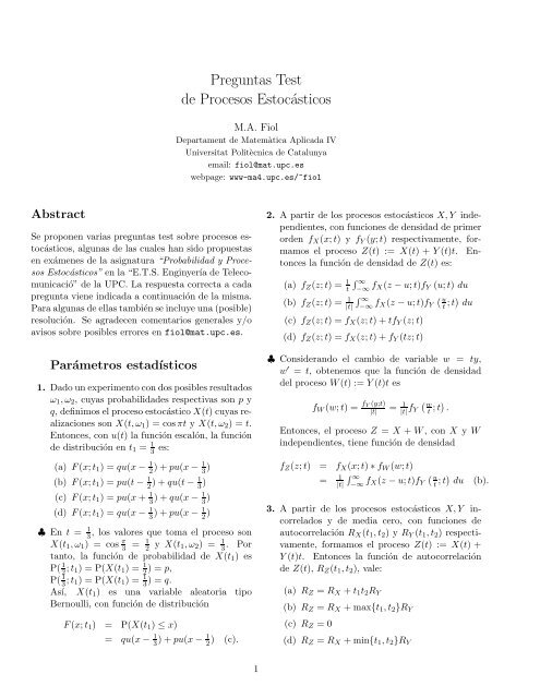
Preguntas Test de Procesos Estocásticos - Departament de ...

Preguntas Test
de Procesos Estocásticos
M.A. Fiol
Departament de Matemàtica Aplicada IV
Universitat Politècnica de Catalunya
email: fiol@mat.upc.es
webpage: www-ma4.upc.es/~fiol
Abstract
varias
algunas
la asignatura
en
UPC.
indicada
ellas
agradecen
posibles
Parámetros
experimento
probabilidades
el proceso
son
con u(t)
distribución
)=qu(x
)=pu(t
)=pu(x
)=qu(x
los
cos
función
1)=P(X(t
1)=P(X(t
es
con
=
=
procesos
propuestas
Procesos
Telecomunicació”
a cada
misma.
(posible)
generales y/o
fiol@mat.upc.es.
resultados
son p
cuyas
ω 2 )=t.
función
proceso son
3 . Por
X(t 1 )
aleatoria tipo
2. A partir de los procesos estocásticos X, Y independientes,
con funciones de densidad de primer
orden f X (x; t) yf Y (y; t) respectivamente, formamos
el proceso Z(t) := X(t) +Y (t)t. Entonces
la función de densidad de Z(t) es:
(a) f Z (z; t) = 1 ∫ ∞
t −∞ f X(z − u; t)f Y (u; t) du
(b) f Z (z; t) = 1 ∫ ∞
|t| −∞ f (
X(z − u; t)f u Y t ; t) du
(c) f Z (z; t) =f X (z; t)+tf Y (z; t)
(d) f Z (z; t) =f X (z; t)+f Y (tz; t)
♣ Considerando el cambio de variable w = ty,
w ′ = t, obtenemos que la función de densidad
del proceso W (t) :=Y (t)t es
f W (w; t) = f Y (y;t)
|t|
= 1
|t| f ( w
Y t ; t) .
Entonces, el proceso Z = X + W ,conX y W
independientes, tiene función de densidad
f Z (z; t) = f X (x; t) ∗ f W (w; t)
= 1 ∫ ∞
|t| −∞ f (
X(z − u; t)f u Y t ; t) du (b).
3. A partir de los procesos estocásticos X, Y incorrelados
y de media cero, con funciones de
autocorrelación R X (t 1 ,t 2 )yR Y (t 1 ,t 2 ) respectivamente,
formamos el proceso Z(t) :=X(t) +
Y (t)t. Entonces la función de autocorrelación
de Z(t), R Z (t 1 ,t 2 ), vale:
(a) R Z = R X + t 1 t 2 R Y
(b) R Z = R X +max{t 1 ,t 2 }R Y
(c) R Z =0
(d) R Z = R X + min{t 1 ,t 2 }R Y
Se proponen preguntas test sobre estocásticos,
Estocásticos” la “E.T.S. Enginyería de de la La respuesta correcta de las cuales han sido
en exámenes de “Probabilidad y
pregunta viene a continuación de la
Para algunas de también se incluye una
resolución. Se comentarios
avisos sobre errores en
estadísticos
1. Dado un con dos posibles
ω 1 ,ω 2 , cuyas respectivas y
q, definimos estocástico X(t) realizaciones
X(t, ω 1 )=cosπt y X(t,
Entonces, la función escalón, la
de en t 1 = 1 3 es:
(a) F (x; t 1 − 1 2 )+pu(x − 1 3 )
(b) F (x; t 1 − 1 2 )+qu(t − 1 3 )
(c) F (x; t 1 + 1 3 )+qu(x − 1 3 )
(d) F (x; t 1 − 1 3 )+pu(x − 1 2 )
♣ En t = 1 3
, valores que toma el
X(t 1 ,ω 1 ) = π 3 = 1 2 y X(t 1,ω 2 ) =
tanto, la de probabilidad de es
P( 1 2 ; t 1 )= 1 2 )=p,
P( 1 3 ; t 1 )= 1 3 )=q.
Así, X(t 1 ) una variable
Bernoulli, función de distribución
F (x; t 1 ) P(X(t 1 ) ≤ x)
1

♣ Al tener media nula, la función de autocorrelación
de X es R X (t 1 ,t 2 ) = E{X(t 1 )X(t 2 )}
y análogamente para Y (t). Además, por
tratarse de procesos incorrelados, C XY (t 1 ,t 2 )=
0 ó, de forma equivalente, E{X(t i )Y (t j )} =
m X (t i )m y (t j ) = 0. Por tanto,
R Z (t 1 ,t 2 ) = E{Z(t 1 )Z(t 2 )}
= E{(X(t 1 )+Y (t 1 )t 1 )
(X(t 2 )+Y (t 2 )t 2 )}
= R X (t 1 ,t 2 )+t 1 t 2 R Y (t 1 ,t 2 ) (a).
4. A partir de una variable aleatoria A con distribución
exponencial de parámetro λ, se define
el proceso estocástico X(t) :=Ae −At . Entonces
su media m(t), t>0, es:
(a) 1/A
(b) 1/λ
(c)
λ
(λ+t) 2
(d)
1
λ+t
♣ La función de densidad de A es f A (a) =λe −λt ,
t>0. Por tanto, utilizando el teorema de la
esperanza,
m X (t) = E(Ae −At )=
=
=
∫ ∞
∫ ∞
0
ae −at λe −λa da
λ
λ + t 0
a(λ + t)e −(λ+t)a da
λ
(λ + t) 2 (c).
donde hemos usado que una v.a. exponencial de
parámetro λ + t tiene media 1/(λ + t).
5. Sea Y una variable aleatoria uniforme en (0, 2).
A partir de ella, se define el proceso
X(t) =
{
Y, 0 ≤ t ≤ Y
0, en otro caso.
La media del proceso en t ∈ (0, 2) es:
♣ Como E{X(t)|Y = y} = y cuando y ≥ t y
E{X(t)|Y = y} = 0 cuando y ≤ t, obtenemos,
para t ∈ [0, 2]:
m X (t) = E{X(t)}
=
=
∫ ∞
E{X(t)|Y = y}f y (y) dy
−∞
∫ 2
y 1 [ ]
y
2 2
t 2 dy = 4
t
( ) t 2
=1− (c).
2
6. Dada la variable aleatoria T uniforme en (0, 2),
se define el proceso
{ t
X(t) = T , 0 ≤ t ≤ T
0, en otro caso.
♣
Entonces la media de X(t) en0

9. Dado un proceso de Poisson con parámetro λt,
se definen las variables aleatorias T 1 y T 2 como
los tiempos transcurridos hasta que se producen
la primera y segunda transición respectivamente.
Entonces se cumple:
♣
(a) E(T 2 |T 1 )=E(T 2 )
(b) E(T 2 |T 1 )= 1 λ + T 1
(c) E(T 1 |T 2 )= 1 λ
(d) E(T 1 |T 2 )= 2 λ − T 2
(b).
10. A partir de un experimento que consiste en lanzar
repetidamente, cada T segundos, una moneda
equilibrada, se define el proceso estocástico
discreto llamado marcha aleatoria de la siguiente
forma: X(0) = 0 y, para n = 1, 2, 3 ...,
X[nT ]=X[(n − 1)T ]+s si sale cara, y
X[nT ]=X[(n − 1)T ] − s si sale cruz.
Entonces, la estadística de primer orden es:
(a) P{X[nT ]=rs} = ( n ) 1 n+r
2
,
2
n
r = −n, −n +2, −n +4,...,n− 2,n
(b) P{X[nT ]=rs} = ( n ) 1 n+r
2
,
2
n
r = −n, −n +1, −n +2,...,n− 1,n
(c) P{X[nT ]=rs} = ( n) 1
r 2
, n
r = −n, −n +2, −n +4,...,n− 2,n
(d) P{X[nT ]=rs} = ( n) 1
r 2
, n
r = −n, −n +1, −n +2,...,n− 1,n
♣
(a).
11. Sea X el proceso estocástico marcha aleatoria
definido en la pregunta anterior. Entonces
sus momentos de primer orden E{X[nT ]} y
E{X 2 [nT ]} son, respectivamente,
(a) ns, ns
(b) ns, ns 2
(c) 0, ns 2
(a) X(t) es estacionario en sentido amplio
(b) Las variables aleatorias X(t 1 )yX(t 2 )son
independientes para todo (t 1 ,t 2 )
(c) X(t) esergódico
(d) Las variables aleatorias X(t 1 ) y X(t 2 )
son incorreladas sólo si E{X(t 1 )} =
E{X(t 2 )} =0
♣ Como K(t 1 ,t 2 ) = 0, las variables aleatorias
X(t 1 )yX(t 2 ) son incorreladas. Por tanto, como
se trata de variables gaussianas, son también independientes.
(b).
Procesos estacionarios
13. Dado un conjunto de 2n variables aleatorias
{A i ,B i ;1≤ i ≤ n} incorreladas, de media cero y
varianza σA 2 i
= σB 2 i
= σi 2 , el proceso estocástico
♣
n∑
X(t) := [A i cos(ω i t)+B i sin(ω i t)]
i=1
es estacionario en sentido amplio, con media cero
y función de autocorrelación:
(a) R X (τ) = ∑ n
i=1 σi 2 cos(ω iτ)
(b) R X (τ) = ∑ n
i=1 σi 2 sin(ω iτ)
(c) R X (τ) = ∑ n
i=1 σi 2 cosh(ω iτ)
(d) R X (τ) = ∑ n
i=1 σ i sin 2 (ω i τ)
(a).
14. Sea X(t) un proceso estocástico estacionario en
sentido amplio, con función de autocorrelación
R X (τ). Entonces, el proceso
Y (t) := 1 [X(t + ɛ) − X(t)], ɛ ∈ R,
ɛ
tiene función de autocorrelación:
♣
(d) 0, ns
(c).
12. Sea X(t) un proceso gaussiano con autocovarianza
K(t 1 ,t 2 ) = 0. Entonces se puede afirmar:
♣
(a) R Y (τ) = 1 ɛ
[2R 2 X (τ) − 2R X (τ − ɛ)]
(b) R Y (τ) = 1 ɛ
[2R 2 X (τ)−R X (τ −ɛ)+R X (τ +ɛ)]
(c) R Y (τ) = 1 ɛ [R X(τ) − R X (τ − ɛ)+R X (τ + ɛ)]
(d) R Y (τ) = 1 [2R
ɛ 2 X (τ)+2R X (τ + ɛ)]
(b).
3

15. Sea X(t) un proceso estocástico estacionario en
sentido amplio y Φ una variable aleatoria independiente
de X(t) con función característica
M Φ (ω) :=E{e jωφ }. Entonces, el proceso
♣
Y (t) :=X(t)sin(ωt +Φ), ω ∈ R,
es estacionario en sentido amplio
(a) sólo si Φ es uniforme en (0, 2π)
(b) si M Φ (1) = 0
(c) sólo si Φ es uniforme en (−π, π)
(d) si y sólo si M Φ (1) = M Φ (2) = 0
(d).
16. Dada la variable aleatoria A uniforme en
(−π, π), se define el proceso estocástico X(t) =
A, t ≥ 0. Entonces se cumple:
(a) El proceso es ergódico en media
(b) La media del proceso es una variable aleatoria
(c) La media temporal (de una realización) es
constante
(d) Ninguna de las anteriores
♣ Una realización del proceso es X(t, ω) =a, t ≥ 0,
a ∈ (−π, π). Por tanto la media temporal es
1
M = lim
T →∞ 2T
∫ T
0
adt= a 2
(c).
17. Considérese el proceso estocástico estacionario
en sentido amplio X(t) :=A cos(ωt + Θ), donde
ω ∈ R y A, Θ son dos variables aleatorias independientes,
y Θ tiene distribución uniforme en
(−π, π). Entonces se puede afirmar que X(t) es
(a) ergódico en media y en autocorrelación
(b) ergódicoenmedia,peronoenautocorrelación
(c) ergódico en autocorrelación, pero no en media
(d) ninguna de las otras
♣ Sea X i (t) =a i cos(ωt + θ i ) una realización del
proceso. Entonces, el cálculo de la media, y media
temporal de X(t) es:
m = E{X(t)}
= E(A)E{cos(ωt +Θ)}
= E(A) 1 ∫ π
cos(ωt + θ) dθ =0;
2π
M = lim
T →∞
= lim
T →∞
−π
∫
a T i
−T
2T
a i
2T
cos(ωt + θ i ) dt
1
ω 2sin(ωT + θ i)=0.
Luego el proceso es ergódico en media.
Análogomente, el cálculo de la autocorrelación y
autocorrelación temporal en t 1 = t 2 = t (τ =0)
da:
R X (0) = E{X 2 (t)}
= E(A 2 )E{cos 2 (ωt +Θ)}
= E(A 2 ) 1 ∫ π
cos 2 (ωt + θ) dθ
2π −π
= 1 2 E(A2 );
a 2 ∫ T
i
R X (0) = lim cos 2 (ωt + θ i ) dt
T →∞ 2T −T
a 2 ∫ T
i 1
= lim
T →∞ 2T 2 [1 + cos(ωt + θ i)] dt
−T
= a2 i
2 .
Por tanto el proceso no es ergódico en autocorrelación
y la respuesta correcta es la (b).
18. La salida de un sistema lineal cuya entrada es
el proceso estacionario X(t) con espectro de potencia
S(f) =F{R X (τ)} es
♣
∫ t
Y (t) = 1 X(τ) dτ.
a t−a
Entonces el espectro de potencia del proceso
Y (t) es:
(a) S Y (f) =S(f) sin2 (πfa)
(πfa) 2
(b) S Y (f) =S(f)cos 2 (πfa)
(c) S Y (f) =S(f) ∣ sin(πfa)
∣
πfa
(d) S Y (f) =S(f)
1
1+(πfa) 2
(a).
Estimación
19. Sean A, B dos variables aleatorias independientes
de media cero y varianza σ 2 . Dado el proceso
estocástico X(t) :=A cos(ωt) +B sin(ωt),
4

♣
la mejor estimación lineal de X(t 1 )dadoX(t 2 ),
donde t 1 ≥ t 2 ,es:
(a) X(t 2 )sin(ωτ)
(b) X(t 2 )+sin(ωτ)
(c) X(t 2 )cosτ
(d) X(t 2 )cos(ωτ)
(d).
20. A partir de las variables aleatorias A, B, independientes
de media cero y varianza σ 2 , formamos
el proceso estocástico X(t) :=At + B.
Entonces la mejor estimación lineal de X(t 1 )
dado X(t 2 ), donde t 1 ≠ t 2 ,es:
♣
(a) X(t1 ̂ )=0
(b) X(t1 ̂ )= 1+t 1t 2
X(t
1+t 2 2 )
2
(c) X(t1 ̂ )= 1+t 1
1+t 2
X(t 2 )
(d) X(t1 ̂ )= t 1t 2
X(t
1+t 2 2 )
2
(b).
21. Sea X(t) un proceso de Poisson de media λt.
Entonces, la mejor estimación lineal de X(t 1 )
dado X(t 2 ), donde t 1 ≥ t 2 ,es:
(a) X(t 2 )+R X (t 1 − t 2 )
(b) X(t 2 )+λt 1
(c) X(t 2 )+λ(t 1 − t 2 )
(d) λt 1
♣
(a)
(b)
(c)
(d)
(b).
̂ X(t1 )=X(t 2 )
̂ X(t1 )=X(t 2 )e −2λ(t 1−t 2 )
̂ X(t1 )=X(t 2 )e −2λ|τ|
̂ X(t1 )=X(t 2 ) − e −2λt 1
24. Sea X(t) el proceso estocástico denominado impulsos
de Poisson, con media m X (t) =λ yautocorrelación
R X (τ) = λ 2 + λδ(τ). Entonces,
la mejor estimación lineal de X(t 1 )dadoX(t 2 ),
t 1 ≠ t 2 ,es:
♣
(a) λt 1
(b) X(t 2 )+λ
(c) λ
(d) X(t 2 )+λt 1
(c).
25. Sea X(t) un proceso de Poisson de media λt.
Dados tres instantes de tiempo t 1 ≥ t 2 ≥ t 3 ,
la mejor estimación lineal homogénea de X(t 2 )
dados X(t 1 )yX(t 3 )es:
♣
(a) t 2−t 1
t 3 −t 1
[X(t 3 ) − X(t 1 )]
(b) X(t 3 ) − λ(t 3 − t 2 )
(c) X(t 1 )+λ(t 2 − t 1 )
(d) t 3−t 2
t 3 −t 1
X(t 1 )+ t 2−t 1
t 3 −t 1
X(t 3 )
(d).
♣
(c).
22. Sea X(t) un proceso de Poisson de media λt.
Entonces, la mejor estimación lineal de X(t 1 )
dado X(t 2 ), donde t 2 ≥ t 1 ,es:
(a) t 2
t1
X(t 2 )
(b) X(t 2 ) − λ(t 2 − t 1 )
♣
(c) λt 1
(d) t 1
t2
X(t 2 )
(d).
23. Sea X(t) el proceso estocástico llamado señal
telegráfica aleatoria, con media m X (t) =e −2λt
y autocorrelación R X (τ) =e −2λ|τ| . Entonces,
la mejor estimación de X(t 1 )dadoX(t 2 ), con
t 1 ≥ t 2 ,es:
5