koff - LEPA

Adsorption in biosensors
1. Adsorption from an infinitely large volume
1.1 Thermodynamic aspects
In most biosensors, the recognition event such as the antigen – antibody reaction or the
oligonucleotide hybridisation occurs between a target molecule in the sample solution and the
receptor adsorbed on a solid support, which can be a microtiter plate, a microbead or a
microarray chip.
To understand, which step controls the binding reaction, we shall consider first the simplest case
where the recognition process is slow compared to the transport in solution, and where the
sample volume is large enough to consider that the reactant concentration is constant.
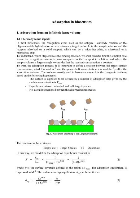
To treat, the adsorption process, it is important to define a relation between the target surface
concentration, noted Γ in mol·m –2 , and the species bulk concentration, c in mol·dm –3 , called the
adsorption isotherm. The isotherm mostly used in biosensor research is the Langmuir isotherm
based on the following hypotheses:
- The surface is supposed to be defined by a number of adsorption sites given by the
surface concentration is Γ max .
- Equilibrium between adsorbed and bulk target species
- No lateral interactions between the adsorbed target species
The reaction can be written as
Fig. 1. Adsorption according to the Langmuir isotherm
Empty site + Target Species ! Adsorbate
In this way, we can define the adsorption equilibrium constant as
K =
kon koff =
!
( ! max " ! ) c bulk
=
!
( 1"! ) c
bulk (1)
where θ is the surface coverage defined as the ration Γ/Γ max . The adsorption equilibrium is
expressed in M –1 . The surface coverage equilibrium ! eq can be written as
! eq =
Kc bulk
1+ Kc bulk
=
"
1+"
(2)

The dimensionless parameter ψ is useful to define the adsorption process. If ψ is much smaller
than unity, then we have an adsorption from a dilute solution where the surface coverage is small
and directly proportional to the bulk concentration; we then speak of the linearized Langmuir
isotherm. If ψ is much greater than unity, then the coverage tends to a full monolayer. When ψ
is equal to unity, the equilibrium coverage is half of the full coverage. In the case of biosensing,
we deal generally with dilute solutions and therefore the equilibrium surface concentration is
directly proportional to the bulk concentration.
! eq = ! max Kc bulk (3)
Exercise : For all the calculations, we shall take K=10 9 M –1 , k on =10 6 M –1 ·s –1 , a bulk analyte
concentration of 0.1 pM unless specified otherwise, and ! max " 10 #9 mol·m #2 .
Calculate the area of an adsorption site, the equilibrium surface coverage and ψ .
1.2 Kinetic aspects
The rate law for a binding reaction is just given by the difference between the adsorption process
considered as a second order reaction between the reactant and a free site and the desorption
process simply considered as a first order reaction, and we can write
d!
dt
= k on c bulk (1!!) ! k off! (4)
This differential equation can be re-arranged as
d!
!
"
dt +! k onc bulk + k off
and the solution is then given by
! =
k on c bulk
k on c bulk + k off
#
$ = konc bulk (5)
1! exp ! konc bulk " " ( + k
#
off )t $ $
#&
% %' =
where τ is the time constant for the adsorption defined as
! =
1
k on c bulk + k off
=
t d
1+"
"
"# 1! exp [ !t /# ] $
1+"
% (6)
where td is the desorption time ( td = 1/ koff ) . This equation clearly shows that the adsorption
kinetics from dilute solutions is controlled by the desorption time.
The adsorption kinetics is illustrated schematically in Figure 2 for different values of ψ
Fig. 2. Time dependence of the surface coverage
(7)
2

Figures 3 & 4 illustrate the dependence of τ on k on and k off .
log ( / s )
log ( / s )
5
4
3
2
1
0
-1
-2
k off = 10 –4
k off = 10 –3
k off = 10 –2
k off = 10 –1
k on = 10 5
-15 -10 -5 0
log (c /M)
Fig. 3. Influence of desorption time koff in s –1 .
5
4
3
2
1
0
-1
-2
k off = 10 –4
k on = 10 6 , 10 5 , 10 4 , 10 3
-15 -10 -5 0
log (c /M)
Fig. 4. Influence of adsorption time kon in M –1 ·s –1 .
At low concentrations, the adsorption time constant is dominated by the desorption rate whilst it
is dominated by the adsorption rate at high concentrations. The transition point on Figures 3 & 4
corresponds to a concentration of K –1 .
We can also define the adsorption time t a = 1/ k onc bulk
( ) such that
! !1 = t a !1 + td !1 (8)
At low bulk concentrations ( !

! = ! eq
t
t d
Exercise : Calculate t a , t d , and τ. Please comment. Plot Γ(t)/Γ eq .
To give some orders of magnitude, Table 1 gives some kinetic values for some classical systems.
k on / M –1 ·s –1 k off / s –1
IgE 10 6 10 –3
IgG4 10 6 10 –2
Avidin-Biotin 10 8 10 –7
ss-DNA 6·10 4 5·10 –5
Exercise : Please comment on the different values
1.3 Adsorption measurement
To monitor the adsorption of target species onto a substrate, one can distinguish label-free
techniques and techniques relying on a chemical labelling step.
Label free techniques include wire conductivity measurements, capacitance measurements,
quartz microbalance measurements, resonators and surface plasmon resonance measurements.
Chemical labelling is used for immunoassays and protein arrays using often a secondary
antibody labelled with an enzyme. Enzyme activity is then monitored by addition of a substrate.
In the case of DNA, the complementary oligo sequence is itself labelled often with a
fluorophore.
Label-free techniques are very useful to measure the kinetics of binding. For example, a flow
system combined to SPR can be used to measure a sensorgram. The measurement is done in two
steps. First, a buffer solution is passed on the detector, and at time t=0, a solution of target
species is injected, the adsorption is then monitored. At a given time, the flowing solution is
switched to the eluent and the desorption is monitored as shown below.
Adsorption
Desorption
Exercise : Please explain the physical principles of a label-free technique (min 1 A4 page).
Derive the equation and draw a sensorgram for the system used above, namely K=10 9 M –1 ,
k on =10 6 M –1 ·s –1 , a bulk analyte concentration of 0.1 pM.
Time
(11)
4

2. Adsorption from a finite volume
2.1 Thermodynamic aspects
In microsystems, the surface to volume ratio can be very large and the bulk concentration can
decrease when the target molecules adsorb. At equilibrium, the bulk concentration and therefore
the equilibrium surface coverage will be different than for large systems having a small S/V ratio.
t = 0 c 0
Adsorption
Equilibrium c eq < c 0
Fig. 5. Adsorption in a microchannel
Another way to increase even further the surface to volume ratio is to fill the channel with
magnetic beads coated by antibodies. In this case, the area corresponds to the total bead area, and
the volume corresponds to the void volume between the beads.
Let’s consider the injection of target molecules in a microchannel, as illustrated in Figure 5. The
number of molecules injected is n in = c inV , where V is the volume of the solution. These
molecules distribute themselves between the walls and the bulk, and if we consider a linearized
Langmuir isotherm, we have:
µ
nin = nwall + nsolution = ! eqA
+ ceqV = K! maxceqA + ceqV (12)
µ
where ! eq is the equilibrium surface concentration in the microchannel, which is related to the
sample concentration by
µ
! eq
=
" K! maxV %
#
$ V + K! maxA &
' cin =
with ! a dimensionless geometric factor, given by
! =
V
AK! max
! eq
1+ K! max A /V = ! ! eq
1+!
We can see that when the volume is large, we recover eq.(3). We can also define a wall
collection efficiency as
! = n wall
n in
= A! eq
µ
Vcin =
K! maxA
V + K! maxA =
1
1+"
We can see that α tends to unity for large surfaces and to zero for large volumes.
(13)
(14)
(15)
5

Exercise: Calculate α and ! for a microchannel 1cm long x100µm wide x 50µm deep, and for
a microtiter plate V = 100µL, A = 1 cm 2 .
50!m
1cm
Example : IgG-Antigen
100!m
K=10 9 M –1
kon=10 6 M –1 ·s –1
100 L = 1cm
V = 50nL
2
2.2 Comparison between a microtiter plate and a microchannel
c bulk = 0.1 pM
A = 3mm 2
Exercise: Please fill the following table Total using well volume the = 300numerical L values listed above:
D=10 –10 m 2 ·s –1
!= 0.01667
Microtiter well Microchannel
A market of more than 20 billion $...
" = 0.9836
Volume ! = 100 "m
100μL
# max = 10 –9 mol·m –2
Initial number of antigens in solution
Surface area 100 mm 2
Maximum antibody sites
Adsorbed antigens
(Maximum)
Enzyme Linked ImmunoSorbent Assay
ELISA
100 L = 1cm 2
Total well volume
DiagnoSwiss Immunochip
Surface = blocking 300 L
Y Y Y Y
# eq $ 10 –6
With one fill, we have only 0.0001% of a
monolayer for a 0.1pM solution
Y Y Y
Y
Y
Y
Y Y Y
Capture antibody adsorption
Wash
Wash
Antigen adsorption
Wash
Counter antibody adsorption
Addition of substrate
Detection
2.3 Kinetic aspects
To estimate the kinetics of adsorption in a microsystem, we can write eq.(4) as
dn wall
n s dt
"
= kon #
$
n in ! n wall
V
%
&
' ns ! n " wall %
#
$
&
' ! k "
off
#
$
n s
n wall
n s
%
&
'
Y Y Y
Y
Y
Y Y Y Y
6
Y
Y Y Y
A market of more than 20
where n s is the total number of sites available on the walls of the microsystem. Implicitly, we
assume that the bulk concentration is homogeneous, i.e. we neglect any mass transport
contribution. By neglecting the second order term, we can re-write this differential equation as
dt + kon nin + n !
s
"
# V
dn wall
The solution of eq.(17) is
n wall =
( )
k onn inn s
( )
V kon nin + n !
s
"
# V
$
+ koff %
& nwall = konninns V
( )
1' exp '
$
+ koff %
&
k ( ( ! on nin + ns * *
"
#
) * ) V
$
+ koff %
& t
+ +
--
, , -
We can re-arrange this equation introducing the geometric factor ! to read
n wall =
( )
nin 1+! ( 1+ Kcin ) 1! exp ! kon nin + n ( ( "
s
* *
#
$
) * ) V
%
+ koff &
' t
+ +
--
, , -
The adsorption time constant in a microsystem τ µ can be compared to that of a planar surface in
a large volume as when n in is much greater than n s the two expressions converge.
(16)
(17)
(18)
(19)

! µ =
1
( )
V
k on n in + n s
+ k off
=
1
kon ( cin + (A /V)! max ) + koff If we still define ψ as equal to Kc in , then when ψ

3. Adsorption on a planar substrate with semi infinite linear diffusion
3.1 General equations
When the rate of adsorption is fast compared to the time scale of diffusion, the kinetics of the
binding may depend on the rate of arrival of the target species to the surface.
To know in which case we operate, it is useful to define a diffusion time as t diff = ! 2 / D , where δ
is the diffusion layer thickness and D the diffusion coefficient. The diffusion layer thickness
varies with time in unstirred solutions, but can be fixed by controlling the hydrodynamics e.g.
flow cells or the geometry e.g. microbeads (steady-state diffusion).
To be able to treat kinetic and mass transport, we shall use the two-layer model, where we define
a volumic surface concentration c surf that differs from the bulk value c bulk such that the diffusion
flux is driven by the gradient (c surf – c bulk )/δ . Indeed, a diffusion flux results from a gradient of
concentration.
By rewriting eq.(4) in terms of the surface concentration Γ and a volumic concentration at the
surface c surf , we have
d!(t)
dt
= konc surf ( ! max " !(t) ) " koff!(t) (22)
Two layer model
!
c
z
surf
Adsorbed layer
Surface layer
Bulk
c bulk
Fig.6. Two-layer model with the adsorbed and the surface layers.
The diffusion equation is given by Fick’s second law, which for a linear geometry reads
!c(x,t)
!t
= D ! 2 c(x,t)
! x 2 (23)
where D is the diffusion coefficient (m 2 ·s –1 ). The variation of the surface concentration of the
target species with time is equal to the flux of arrival at the surface:
d!(t)
dt
= D !c(x,t) " %
#
$
! x &
'
x=0
= ( J(t) (24)
8

Unfortunately, these equations cannot be solved analytically in the general case, but specific
solutions can be obtained for example assuming that the diffusion process is steady-state.
3.2 Steady-state approximation for kinetic-diffusion control at short times
Here, we consider the simple case based on neglecting the presence of occupied sites, i.e.
!

!(t) =
konc bulk "
%
$ ! '
max
$
' t
$
2t
1+ k '
# on! max
D &
=
" t % 1
! eq
#
$ td &
'
1+ kon! max
Figure 7 shows a surface concentration-time plot showing the influence of the diffusion in stirred
and unstirred solutions.
Exercise : Please plot Γ(t)/Γ eq using D = 10 –10 m 2 ·s –1 and δ = 100µm. Please also calculate the
Damköhler number.
Γ /Γ eq
0.6
0.5
0.4
0.3
0.2
0.1
0.0
0
Kinetic control
Kinetic-Steady state diffusion
Kinetic-Time dependent
diffusion layer thickness
200
400
Fig. 7. Influence of the diffusion on the adsorption. ( K=10 9 M –1 , kon=10 6 M –1 ·s –1 , c bulk = 0.1 pM,
t /s
600
2t
D
800
1000
D=10 –10 m 2 ·s –1 , δ = 100 µm and ! max " 10 #9 mol·m #2 ). θ

3.3 Steady-state approximation for kinetic-diffusion control in dilute solutions
( ) ,
When the surface concentration is proportional to the volumic surface concentration !

Γ /Γ eq
1.0
0.8
0.6
0.4
0.2
0.0
0
2000
4000
Kinetic-Steady state diffusion
Diffusion control
Kinetic-Time dependent
diffusion layer thickness
t /s
6000
8000
10000
Fig. 8. Comparison between stirred and unstirred diffusion controlled reactions . ( K=10 9 M –1 ,
kon=10 6 M –1 ·s –1 , c bulk = 0.1 pM, D=10 –10 m 2 ·s –1 , δ = 100 µm and ! max " 10 #9 mol·m #2 ).
This figure shows that the perturbation theory gives a rather good approximation to the exact
solution eq.(38).
3.4 Steady-state approximation for kinetic-diffusion control - General case
Eq.(26) can be more generally written as
d!(t)
dt
= konc surf ! max ( 1"! ) " koff! max! = " J = D
or in terms of surface coverage
d!(t)
dt
= konc surf ( 1!! ) ! koff! =
D
!" max
( ) (40)
! cbulk " c surf
c bulk ! c surf ( ) (41)
from which we can as before obtain an expression for the surface concentration
c surf
( )
( )
= cbulk + Da ! / K
1+ Da 1!!
The differential equation (41) now reads
or
d!(t)
dt
=
( )
konc bulk ( + Dakoff ! ) ( 1!! )
( )
1+ Da 1!!
" 1+ Da 1!! %
$
'd! =
# ! !" ( ! +1)
&
dt
td ( )
! koff! = koncbulk !! konc bulk + koff 1+ Da 1!!
( )
We can integrate this expression explicitly assuming no initial coverage to get
Da! ! 1+ Da " % " " " +1%
%
#
$ " +1&
' ln 1!!
#
$
#
$ " &
'
&
'
( )
t " +1
=
td (42)
(43)
(44)
12

We can either plot the time as a function of the surface coverage or see different limiting cases to
recover the previous approximations.
Γ /Γ eq
1.0
0.8
0.6
0.4
0.2
0.0
0
500
1000
1500
t /s
2000
ψ =0.1
ψ =1
ψ =10
Figure 9. Comparison between kinetic control under ideal stirring (full line) and with some
diffusion influence according to eq.(44) (dotted line). Da = 1, t d =1000s.
We define a diffusion time as t diff = ! 2 / D , where δ is the diffusion layer thickness and D the
diffusion coefficient.
Exercise: If δ = 100 µm and D = 10 –10 m 2 ·s –1 , calculate t diff and compare with t a and t d . Compare
this general solution with the two approximations, namely at short times and for dilute solutions.
2500
3000
13

4. Adsorption-diffusion in microsystems
4.1 Steady-state approximation
Let us consider a microchannel of height 2h.
2h
l
L
By symmetry, the diffusion layer thickness is h as the top molecules diffuse to the top plate and
the bottom ones to the bottom plates.
We can therefore write the diffusion equation as in eq.(26) as
d!(t)
dt
= konc surf ! max = " J = D
! cbulk " c surf ( ) (45)
To take in to account the depletion in the center of the channel upon adsorption as in equation
(16) reproduced below
dn wall
n sdt
"
= kon #
$
n in ! n wall
V
and the diffusion equation reads
d!(t)
dt = dnwall Adt = kon "
#
$
n surf
V
%
&
' ns ! n " wall %
#
$
&
' ! k "
off
#
$
n s
%
&
' ! max = D "
! #
$
As in equation (27), we can express nsurf as
nsurf = nin ! nwall kon " max!
+1
D
We can now solve the differential equation
dn wall
dt
= Ak on ! max
V
#
$
%
The solution of this equation is
n wall
n s
%
&
'
n in ( n wall ( n surf
V
%
&
'
(46)
(47)
= n in ! n wall
Da +1 (48)
n in " n wall
Da +1
&
'
( == 1
( " t % +
nwall = nin * 1! exp !
#
$ !td ( Da +1)
&
' -
) *
, -
!t d
#
$
%
n in " n wall
Da +1
When Da>>1, we are diffusion controlled with a fast kinetic, we have
( " t % +
nwall = nin * 1! exp !
#
$ !tdDa &
' -
)
,
&
'
(
(49)
(50)
(51)
14

and when the mass transport is fast, we recover nearly eq.(21)
nwall = nin 1! exp ! t
( "
*
#
$
)
!t d
% +
&
' -
,
Exercise : Calculate the number of antigens adsorbed in the same microchannel as above after 30
s and compared to the number one would reach at equilibrium. Please comment.
4.2 Comparison between a microtiter plate and a microchannel
Discuss the differences between a microtiter plate and a microchannel.
Please fill the following table using the numerical values listed above taking into account the
diffusion:
Volume 100μL
Initial number of antigens in solution
Adsorbed antigens
(Maximum)
Adsorbed antigens
After 3 min
Adsorbed antigens
After 15 min
Adsorbed antigens
After 10 s
Adsorbed antigens
After 30 s
Microtiter well Microchannel
XXXXX
XXXXX
XXXXX
XXXXX
(52)
15

5. Coating a microchannel
5.1 Iterative stop-flow with adsorption equilibrium
One way to coat a microchannel is the stop-flow method that consists in filling the channel
quickly and to allow the adsorption to take place. This process is then repeated n-times until the
surface concentration is high enough to allow a detection using, for example, a sandwich assay.
During the iterative process, the total number of molecules present after the nth fill of the
microchannel channel is equal to what was adsorb on the wall at the (n-1) fill plus the number of
molecules injected during the nth fill
n tot,N = n wall, N –1 + n in (53)
In this way, we can write for the successive iterations.
First fill:
Second fill:
n tot,1 = n in (54)
n wall, 1 = !n in (55)
ntot,2 = nwall, 1 + nin = ( 1+ ! )nin (56)
µ
ntot,2 = nwall,2 + nsolution = ! eq,2A
+ ceqV = K! maxceqA + ceqV (57)
µ
! eq,2
=
" K! max %
#
$ V + K! maxA &
' ntot,2 µ
nwall,2 = ! eq,2A
=
" K! maxA %
#
$ V + K! maxA &
' ntot,2 (58)
= ! 1+ ! ( )nin (59)
Then, at the n-th fill we have
ntot,n = nwall, n!1 + nin = 1+ ! + ! 2 +... + ! n–1
( )nin (60)
and
nwall,n = ! + ! 2 +... + ! n–1
( ) · nin (61)
Considering the properties of geometric series
n wall,N
n in
N –1
!
i=0
= ! 1"! N
= = ! ! i
( )
1"!
As illustrated in Figure 10, we have an additive filling for the values of α close to unity.
(62)
16

n wall / n in
15
10
5
0
0
5
! = 0.99
10
N
Fig. 10. Iterative filling
! = 0.9
15
! = 0.8
! = 0.7
The advantage of the stop-flow method is to guarantee a homogeneous coating of the wall.
Exercise: With previous parameters, calculate how many fills are required to coat a
microchannel with 100’000 antigens and estimate the time required, the sample volume
consumption and the number of analyte molecules wasted.
5.2 Iterative stop-flow with kinetic control
To estimate the kinetics of adsorption in a microsystem, we can write
dn wall
n s dt
( )
V
" nin ! nwall ! n0 % "
= kon #
$
&
'
#
$
n s ! n wall
n s
%
&
' ! k "
off
#
$
where n s is the total number of sites available on the walls of the microsystem, and n0 the
number of molecules adsorbed from the previous step. Implicitly, we assume that the bulk
concentration is constant, i.e. we neglect any mass transport contribution. We can re-write this
differential equation as
dt + kon nin + ns + n !
0
"
# V
dn wall
which gives that
( )
nwall = n0 exp ! k ( " on nin + ns + n0 *
#
$
) V
n wall
n s
$
+ koff %
& nwall = kon nin + n0 V
( )
( )n s
kon nin + n0 +
V k " on nin + ns + n0 #
$ V
( )
%
+ koff &
' t
+
-
,
20
%
&
'
( )n s
( )
1! exp !
%
+ koff &
'
k ( ( " on nin + ns + n0 * *
#
$
) * ) V
We can re-arrange this equation introducing the geometric factor ! to read
%
+ koff &
' t
+ +
--
, , -
(63)
(64)
(65)
17

( )
nwall = n0 exp ! k ( " on nin + ns + n0 *
#
$
) V
nin + n0 +
1+! + K! cin + c0 %
+ koff &
' t
+
-
,
( ) 1! exp ! k ( ( " on ( nin + ns + n0 )
* *
#
$ V
) *
)
%
+ koff &
' t
+ +
--
, , -
The adsorption time constant in a microsystem τ µ can be compared to that of a planar surface in
a large volume as when n in is much greater than n s the two expressions converge.
! µ =
1
( )
V
k on n in + n s + n 0
+ k off
=
t d
( ) =
1+! !1 + K c in + c 0
If we still define ψ as equal to Kc in , then when ψ

progressively along the channel. If the binding kinetics is slow, the coating will be more
homogeneous but it is important not to flow to fast, not too waste too many target species.
As developed in Annexe 2, under pure diffusion control the diffusion layer thickness in a flow
channel varies with the flow rate according to
! =
∫
l
3
0
3a 2 Dx
dx
!
0
l
∫ dx
=
∫
l
3
0
0.759Dhx
dx
< v >
l
∫ dx
0
=
3
4
0.759Dh
< v >
l
3 l 4/3
The flux of the target species to the wall of a microchannel of length l, of width L, of half height
h where the average liquid velocity is is expressed by
J = 0.8131 c b LD 2/3 l 2/3 < v > 1/3 h !1/3 (73)
Please fill the following table and comment
Linear speed
cm/s
0.01
0.1
1
10
Flow rate
nL/min
δ/μm
nadsorbed
during 1 min
Which flow rate is required to obtain a homogeneous coating along the channel?
(72)
nin
during 1 min
Compared how long it would take to immobilize 100’000 target species under pure kinetic
control and pure diffusion control.
5.4 How to fill a microchannel?
What is the best way to coat a microchannel, with continuous flow or by iterative filling?
19

6. Adsorption-diffusion on a spherical substrate
Nowadays, most immunoassays take place on magnetic beads as illustrated in Figure 11.
Fig. 11. Immunoassay on a magnetic bead
An interesting property of spherical diffusion is to provide a finite diffusion layer thickness. This
property is used in electrochemistry with microelectrodes that can generate steady-state currents
in the absence of any hydrodynamics.
The diffusion layer thickness is equal to the radius R of the substrate.
Exercise : Please demonstrate
For ψ >1, we can use eq.(29), which shows that the surface concentration increases linearly with
time
!(t) =
konc bulk ! max
1+ kon ! maxR "
%
$
'
$
'
t =
#
$
D &
'
" ! eq % t
#
$ 1+ Da&
'
The smaller the beads, the less important the diffusion. It is then only controlled by the kinetics.
For ψ

7. ELISA assay (from www.interferonsource.com)
“Enzyme Linked Immuno-Sorbent Assay (ELISA) is a powerful technique for detection and
quantitation of biological substances such as proteins, peptides, antibodies, and hormones. By
combining the specificity of antibodies with the sensitivity of simple enzyme assay, ELISA can
provide a quick and useful measurement of the concentration of an unknown antigen or
antibody. Currently, there are three major types of ELISA assays commonly used by researchers.
They are: indirect ELISA, typically used for screening antibodies; sandwich ELISA (or antigen
capture), for analysis of antigen present; and competitive ELISA, for antigen specificity”.
Figure 14. Elisa scheme http://www.interferonsource.com/New_InterferonSource/ELISA/ELISA_Description.html,
TetraMethylBenzidine for oxidation by HRP
“The "sandwich" technique is so called because the antigen being assayed is held between two
different antibodies. In this method:
1. Plate is coated with a capture antibody.
2. Sample is then added, and antigen present binds to capture antibody.
3. The detecting antibody is then added and binds to a different region (epitope) of the
antigen.
4. Enzyme linked secondary antibody is added and binds to the detecting antibody.
5. The substrate is then added and the reaction between the substrate and the enzyme
product can be monitored optically or electrochemically.
6. The signal generated is directly proportional to the amount of antibody bound antigen.
Optimizing an ELISA assay requires the careful selection of antibodies and enzyme-substrate
reporting system. Once optimized, sandwich ELISA technique is fast and accurate. If a purified
antigen standard is available, this method can be used to detect the presence and to determine
the quantity of antigen in an unknown sample. The sensitivity of the sandwich ELISA is
dependent on 3 factors:
a) The number of molecules of the first antibody that are bound to the solid phase,
namely, the microtiter plate.
b) The avidity of the antibodies (both capture and detection) for the antigen
c) The specific activity of the detection antibody that is in part dependent on the number
and type of labelled moieties it contains. It is important to note that while an ELISA assay is a
useful tool to detect the presence and the quantity of an antigen in the sample, it does not
21

provide information concerning the biological activity of the sample. ELISAs are not generally
used to discriminate active or non-active forms of a protein. It may also detect degraded proteins
that have intact epitopes”.
8. Protein array (from Arrait.com)
“Antibody, Antigen, Peptide and other Protein Microarrays Custom Made to Order. Antibody
microarrays to Cancer, Apoptosis, Growth Factors, Cytokines, Receptors and More... Users can
to assay thousands of specific proteins with the ArrayIt Protein Microarrays. A wide variety of
proteins representing a range of biological functions are detectable. ArrayIt microarrays allow
users to measure differences in protein abundance using a two-color fluorescent labeling
technique that can be provided with the microarrays. “Sandwich” detection schemes can also be
implemented, please discuss your application goals with us. Detection is typically fluorescentbased
using microarray scanners, but microarrays for other detection platforms can be
provided. The protocols are simple, and the detection limits are extremely high.
Figure 15. Protein array scheme
http://www.arrayit.com/Products/Microarrays/
Figure 15. Two color antibody microarray. Compare two biological samples to measure the absolute and relative
differences in protein expression. This procedure is fluorescence-based and compatible with all current microarray
scanners. Extracted proteins are directly labelled (kit provided) and analysed. The covalently immobilized
antibodies capture fluorescently labelled antigens during the reaction step. Normal and cancerous cells can be
compared. The raw data provide a measure of proteins from samples A & B.
22

9. Redox detection in a microchannel
Most immunoassays use an optical detection method based either on colorimetry, fluorescence
or nowadays more and more chemiluminescence. In ELISA assays, an enzyme reaction takes
place that produce often by cleavage an optical probe.
Fig 16 : Gravicell from DiagnoSwiss SA
The Michaelis-Menten equation for an enzyme reaction is rarely expressed in its explicit form
that gives the product concentration as a function of time
–[P] + KM ln [S ! 0] – [P] $
#
" [S
&
0] %
= ' vmt (76)
At short times, we can linearize this equation
–[P] ! K M
[P]
[S 0 ] = ! v m t
to obtain
vmt [P]=
1+ KM / [S0 ]
(78)
In the case of excess substrate concentration, this equation reduces to
[P]=v mt (79)
In the case of immune-assays with electrochemical detection, the enzyme reaction produces a
redox active probe. In the example below, alkali phosphatase is used to cleave paraaminophenolphosphate
(PAPP) to produce para-aminophenol (PAP) that can be oxidized to
quinone-imine. By amperometry, the current is directly proportional to the PAP concentration
(77)
23

NH2
O
PO 3 2-
ALP,
H2O
pH = 9
NH 2
OH
PAPP AP
+ HPO 4 2-
NH 2
OH
2e -
2H +
NH
O
AP QI
I [A]
8.0E-09
7.0E-09
6.0E-09
5.0E-09
4.0E-09
3.0E-09
2.0E-09
1.0E-09
2 pM
1 pM
0.0E+00
0 pM
0
-1.0E-09
200 400 600 800 1000 1200 1400 1600
Time [s]
Fig 17 : Amperometric detection with PAPP, and PAP oxidation
Ag Concentration
In the case of an oxidation of microdisc electrode, the current is equal to 4nFDcr, where n is the
number of electrons exchanged, F is the Faraday constant, D the diffusion coefficient of the
redox probe, c its concentration and r the radius of the microdisc electrode.
Exercise : Assume a Michaelis-Menten rate law, and calculate the number of PAP molecules
produced as a function of time. Calculate the current one would get on a 25 µm Ø gold disc
microelectrodes. How many electrodes can one fit in the microchannel?
In the literature, we can find k2= 50 s –1
10 pM
24

Annexe 1: ψ

c(x, s) = cbulk
s
!
c bulk
# 1
+
$
% K" max
s &
D '
(
1
sD exp!
In this way, the transform of the concentration at the surface is
c(0, s) = cbulk
s
Knowing the following inverse transform
we have
with
or
!
{ } =
L exp(u 2 t)erfc(u t )
c bulk
# D &
s + s
$
% K" max '
(
1
s s + u
c surf (t) = c bulk 1! exp(a 2 "
#
Dt)erfc(a Dt ) $
%
a =
1
K! max
!(t) = ! eq 1" exp(a 2 #
$
Dt)erfc(a Dt ) %
&
s
D x
A1.9
A1.10
( ) A1.11
A1.12
A1.13
A1.14
It is important to realise that the term in brackets depends only on the adimensional term u =
a 2 Dt as shown below, which in terms depends only on the physical parameters K, Γ max and D,
but not on the bulk concentration. The latter affects only Γ eq .
Fig.8. Illustration of equation Error! Reference source not found.
The transform of the flux using eq.(A1.4) is
"
J (s) = ! D
#
$
!c(x, s)
! x
%
&
'
x=0
=
c D
( a D + s)
A1.15
26

which gives
J(t) = c D 1
!t ! a D expa2 "
Dt %
$
erfc(a Dt ) '
#
&
This expression of the flux can be compared to the Cottrell equation in chronoamperometry
JCottrell(t) = c D 1 ! $
#
" !t
&
%
A1.16
A1.17
We can therefore see that for small values of a D , i.e. large K values or for a large specific
surface area providing a large Γ max or even for small molecules with a small diffusion
coefficient, the Cottrell equation is a good approximation.
Exercise: Derive the equivalent of the Cottrell equation by the perturbation method of a steadystate
flux.
27

Annexe 2: Laminar flow. The Grätz problem
We shall consider here a solution flowing parallel to two plane onto which molecules are
adsorbed on a section of length l as shown in Figure 13. The problem is analogous to the current
obtained in a band electrode in a flow channel.
The equation of flux conservation is given by
!c
!t
Fig. 13. Adsorption in a flow channel
= " divJ = D# 2 c " v·gradc A2.1
In steady state, for a 2D system where the x axis is parallel to the electrode and the y axis
perpendicular to it, we have only
v x
!c
!x + v !c
y
!y = D !2c !y 2 + !2c !x 2
" %
$ '
# &
( D !2c !y 2
A2.2
by neglecting the longitudinal diffusion. The continuity equation for an incompressible fluid is
classically given by
!vx !x + !vy !y
= div(!v) = 0 A2.3
We can solve this equation by doing a series development on y, to obtain
and
with
vx = vx (y = 0) + y !v " x %
#
$
!y &
vy = vy(y = 0) + y !v " y %
#
$
!y &
= 1 2 y2 !
"
!y #
$
!v y
!y
= ( 1 2 y2 ! "
!x #
$
%
&
'
y=0
!v x
!y
%
&
' y=0
+... = y!(x) A2.4
"
' +
y=0
1 2 y2 !2vy !y 2 $
#
%
'
&
+... = ( 1 2 y2 ! "
!y #
$
y=0
!v x
!x
+...
%
&
' y=0
' +... = (
y=0
1 2 y2 ! '(x) +...
+...
A2.5
28

and since
!(x) =
"
#
$
!v y
!y
assuming that
%
&
'
y=0
"
#
$
!v x
!y
%
&
' y=0
= ( !v " x %
#
$
!x &
'
y=0
A2.6
= ( ( y! '(x) ) = 0 A2.7
y=0
v x (y = 0) = v y (y = 0) = 0 A2.8
The flux conservation equation (1.90) becomes
y!(x) !c
!x " y2 ! '(x) !c
2 !y = D !2c !y 2
If the flow is parallel to the wall such that v y is zero, then equation (1.98) reduces to
y!(x) !c
!x = D !2 c
!y 2
A2.9
A2.10
For a Poiseuille flow profile between two planes located at –h and h, the velocity profile is
given by
"
$
#
v x = v max 1!
2
Y
h 2
%
'
&
= 3 < v >
2
2
Y
1!
h 2
" %
$ '
# &
with Y = y ! h , and then β(x) is constant and equal to 3/h.
Equation (1.99) can then be written
D !2 c
!y 2
= 3 < v >
h
Fig. 14. Diffusion layer thickness in flow channels
y !c
!x = 2vmax y
h
!c
!x
A2.11
A2.12
29

Diffusion layer thickness: Approximate solution
To solve equation (1.99), we can consider the thickness of the diffusion layer δ (x) as illustrated
above, and linearize the gradients and write
y! !c
!x
!c dy
= y!
!y dx
#c dy
" y!
#y dx
#c d"
= "!
" dx
with y = ! (x) and !c = c b " c( x = 0).
Similarly, we have
D !2 c
!y 2
" D ! #c
!y #y
= D #c
! 2
With these simplifications, eq.(1.99) reduces to
! d"
dx
= D
" 2
that we can integrate to have
= !#c d"
dx
A2.13
A2.14
A2.15
! 3 = 3Dx
" A2.16
The limiting current on the band electrode is then for the case illustrated in figure 13
I = nFDLc b l dx
0 ! (x)
! = nFDLc b l
0
dx
3
By substituting the value of β equal to 3/h.
or
3Dx
"
= 3 –1/3 nFc b LD 2/3 " 1/3 l 2/3
! A2.17
I = nFc b LD 2/3 l 2/3 < v > 1/3 h !1/3 A2.18
I =
! 2$
"
#
3%
&
1/3
nFc b L vmaxD 2 l 2 !
#
"
h
$
&
%
1/3
!
#
"
= 0.8735nFc b L v maxD 2 l 2
We can write this equation as a function of the volumetric flow rate FV given by
h
$
&
%
1/3
A2.19
F V = 2 < v > hd A2.20
and obtain an equation.
"
$
#
I = 2 !1/3 nFc b L D2 l 2 F V
h 2 d
%
'
&
1/3
"
$
#
= 0.7937 nFc b L D2 l 2 F V
Diffusion layer thickness: Exact solution
We can solve analytically eq.(1.99), by using a similarity variable and write
! y $
c(x, y) = F
"
#
! (x) %
&
The boundary conditions are
h 2 d
%
'
&
1/3
A2.21
= F ( ! ) A2.22
30

or
c(0, y) = c(x, !) = c
c(x, 0) = 0
! y $
c(0, y) = F
"
#
! (0) %
&
c(x, 0) = F( 0)
= 0
The partial derivatives are then
!c
!x
!c
!y
! 2 c
!y 2
!! dF
=
!x d!
!! dF
=
!y d!
=
! " !! dF %
!y #
$
!y d! &
'
= F( ')
= c
y
= "
" 2
# d" &
$
%
dx '
( dF
d!
1 dF
=
" d!
1 !
=
" !y
" dF %
#
$
d! &
'
! d" dF
= "
" dx d!
The two variables differential equation (1.99) becomes
d 2 F
d! 2
! $
#
" %
!
& +!2 "# 2
#
"
D
d# $
dx
&
%
dF
d!
1 !! d " dF %
=
" !y d! #
$
d! &
' =
1
" 2
d 2 F
d! 2
" %
$ '
# &
A2.23
A2.24
A2.25
A2.26
A2.27
= 0 A2.28
The term in brackets must be constant with respect to x and we can write
!" 2 ! d" $
#
" D dx
&
%
= a2 A2.29
We should therefore solve the following equation
d 2 F
d! 2
! $
# &
" %
+ a2 ! 2 dF
d!
A solution of this equation is
since
and
= 0 A2.30
F(!) = c1 exp ! a2
3 z3
" %
$ '
# &
dz + c !
( 0
2
A2.31
F '(!) = c1 exp ! a2
3 !3
" %
$ '
# &
F ''(!) = ! c1a 2 ! 2 exp ! a2
3 !3
" %
$ '
# &
A2.32
A2.33
The integration constants of equation (1.120) must satisfy the boundary conditions (1.113), such
that
31

and
c 2 = 0 A2.34
c1 = c / exp ! a2
3 z3
" %
$ '
# &
dz
(
) A2.35
0
Equation (1.120) becomes
F(!) = c
(
(
!
0
)
0
exp ! a2 "
$
#
exp ! a2 "
$
#
3 z3
3 z3
%
'
&
dz
%
'
&
dz
The normalising integral is finite and equal to
exp ! a2
3 z3
" %
$ '
# &
dz
(
) =
0
2 3
9
5/6
a 2/3 * 2 " %
#
$
3&
'
The concentration profiles are therefore given by
! y $
c(x, y) = F
"
#
! (x) %
&
= F(") =
To calculate the thickness of the diffusion layer, we can write
and
" !c%
#
$
!y&
'
y=0
! dF $
"
#
d! %
& !=0
= !! " dF %
!y #
$
d! &
'
!=0
=
3 1/6 a 2/3 ' 2 ! $
"
#
3%
& c b
2
= 1 " dF %
" #
$
d! &
'
!=0
This equation allows us to calculate a= 0.87116.
By integration of eq.(1.118), we have
! =
∫
l
3
0
3a 2 Dx
dx
!
0
l
∫ dx
=
A2.36
A2.37
3 1/6 a 2/3 c' 2 ! $
"
#
3%
&
exp (
2
a2
3 z3
! $
# &
" %
dz
"
) A2.38
0
= (c
"
= cb
"
A2.39
= 0.8131 a 2/3 c b = c b A2.40
∫
l
3
0
0.759Dhx
dx
< v >
l
∫ dx
0
=
3
4
0.759Dh
< v >
l
3 l 4/3
The limiting current on the band electrode is then for the case illustrated in figure 13
I = nFDLc b l dx
0 ! (x)
! = nFDLc b l
!
0
dx
3
3a 2 Dx
"
= 3 –1/3 a "2/3 nFc b LD 2/3 " 1/3 l 2/3
A2.41
32

By substituting the value of β equal to 3/h.
A2.42
I = a !2/3 nFc b LD 2/3 l 2/3 < v > 1/3 h !1/3 = 0.8131nFc b LD 2/3 l 2/3 < v > 1/3 h !1/3 A2.43
We can write this equation as a function of the volumetric flow rate FV given by eq.(1.109) and
obtain an equation similar to equation (7.50) from the book “ Analytical & Physical
electrochemistry”.
"
$
#
I = 2 !1/3 a !2/3 nFc b L D2 l 2 F V
h 2 d
As a function of the maximum velocity, we have
"
#
$
I = a !2/3 nFc b LD 2/3 l 2/3 2v max
"
$
#
= 1.0744nFc b L v maxD 2 l 2
h
3
%
'
&
%
'
&
1/3
1/3
%
&
'
"
$
#
= 0.6454 nFc b L D2 l 2 F V
1/3
h !1/3 =
" 2%
#
$
3&
'
h 2 d
%
'
&
1/3
1/3
a !2/3 nFc b L vmaxD 2 l 2 "
$
#
h
%
'
&
A2.44
1/3
A2.45
33