5128_Ch04_pp186-260

Create successful ePaper yourself
Turn your PDF publications into a flip-book with our unique Google optimized e-Paper software.
Section 4.5 Linearization and Newton’s Method 233<br />
What you’ll learn about<br />
• Linear Approximation<br />
• Newton’s Method<br />
• Differentials<br />
• Estimating Change with<br />
Differentials<br />
4.5<br />
Linearization and Newton’s Method<br />
Linear Approximation<br />
In our study of the derivative we have frequently referred to the “tangent line to the curve”<br />
at a point. What makes that tangent line so important mathematically is that it provides a<br />
useful representation of the curve itself if we stay close enough to the point of tangency.<br />
We say that differentiable curves are always locally linear, a fact that can best be appreciated<br />
graphically by zooming in at a point on the curve, as Exploration 1 shows.<br />
• Absolute, Relative, and<br />
Percentage Change<br />
• Sensitivity to Change<br />
. . . and why<br />
Engineering and science depend<br />
on approximations in most practical<br />
applications; it is important to<br />
understand how approximation<br />
techniques work.<br />
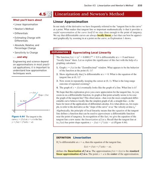
0<br />
y<br />
(a, f(a))<br />
a<br />
y f(x)<br />
Figure 4.44 The tangent to the<br />
curve y f x at x a is the line<br />
y f a f ax a.<br />
Slope f'(a)<br />
x<br />
EXPLORATION 1<br />
Appreciating Local Linearity<br />
The function f (x) (x 2 0.0001) 1/4 0.9 is differentiable at x 0 and hence<br />
“locally linear” there. Let us explore the significance of this fact with the help of a<br />
graphing calculator.<br />
1. Graph y f (x) in the “ZoomDecimal” window. What appears to be the behavior<br />
of the function at the point (0, 1)?<br />
2. Show algebraically that f is differentiable at x 0. What is the equation of the<br />
tangent line at (0, 1)?<br />
3. Now zoom in repeatedly, keeping the cursor at (0, 1). What is the long-range<br />
outcome of repeated zooming?<br />
4. The graph of y f(x) eventually looks like the graph of a line. What line is it?<br />
We hope that this exploration gives you a new appreciation for the tangent line. As you<br />
zoom in on a differentiable function, its graph at that point actually seems to become<br />
the graph of the tangent line! This observation—that even the most complicated differentiable<br />
curve behaves locally like the simplest graph of all, a straight line—is the<br />
basis for most of the applications of differential calculus. It is what allows us, for example,<br />
to refer to the derivative as the “slope of the curve” or as “the velocity at time t 0 .”<br />
Algebraically, the principle of local linearity means that the equation of the tangent<br />
line defines a function that can be used to approximate a differentiable function<br />
near the point of tangency. In recognition of this fact, we give the equation of the<br />
tangent line a new name: the linearization of f at a. Recall that the tangent line at<br />
(a, f (a)) has point-slope equation y f (a) f (x)(x a) (Figure 4.44).<br />
DEFINITION<br />
Linearization<br />
If f is differentiable at x a, then the equation of the tangent line,<br />
L(x) f (a) f (a)(x a),<br />
defines the linearization of f at a. The approximation f (x) L(x) is the standard<br />
linear approximation of f at a. The point x a is the center of the approximation.