5128_Ch04_pp186-260

Chapter
4
Applications of
Derivatives
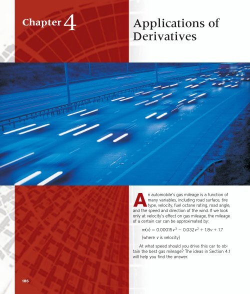
An automobile’s gas mileage is a function of
many variables, including road surface, tire
type, velocity, fuel octane rating, road angle,
and the speed and direction of the wind. If we look
only at velocity’s effect on gas mileage, the mileage
of a certain car can be approximated by:
m(v) 0.00015v 3 0.032v 2 1.8v 1.7
(where v is velocity)
At what speed should you drive this car to obtain
the best gas mileage? The ideas in Section 4.1
will help you find the answer.
186

Chapter 4 Overview
Section 4.1 Extreme Values of Functions 187
In the past, when virtually all graphing was done by hand—often laboriously—derivatives
were the key tool used to sketch the graph of a function. Now we can graph a function
quickly, and usually correctly, using a grapher. However, confirmation of much of what we
see and conclude true from a grapher view must still come from calculus.
This chapter shows how to draw conclusions from derivatives about the extreme values
of a function and about the general shape of a function’s graph. We will also see
how a tangent line captures the shape of a curve near the point of tangency, how to deduce
rates of change we cannot measure from rates of change we already know, and
how to find a function when we know only its first derivative and its value at a single
point. The key to recovering functions from derivatives is the Mean Value Theorem, a
theorem whose corollaries provide the gateway to integral calculus, which we begin in
Chapter 5.
4.1
What you’ll learn about
• Absolute (Global) Extreme Values
• Local (Relative) Extreme Values
• Finding Extreme Values
. . . and why
Finding maximum and minimum
values of functions, called optimization,
is an important issue in
real-world problems.
Extreme Values of Functions
Absolute (Global) Extreme Values
One of the most useful things we can learn from a function’s derivative is whether the
function assumes any maximum or minimum values on a given interval and where
these values are located if it does. Once we know how to find a function’s extreme values,
we will be able to answer such questions as “What is the most effective size for a
dose of medicine?” and “What is the least expensive way to pipe oil from an offshore
well to a refinery down the coast?” We will see how to answer questions like these in
Section 4.4.
DEFINITION Absolute Extreme Values
Let f be a function with domain D. Then f c is the
(a) absolute maximum value on D if and only if f x f c for all x in D.
(b) absolute minimum value on D if and only if f x f c for all x in D.
y cos x
– ––
2
Figure 4.1 (Example 1)
1
0
–1
y
–– 2
y sin x
x
Absolute (or global) maximum and minimum values are also called absolute extrema
(plural of the Latin extremum). We often omit the term “absolute” or “global” and just say
maximum and minimum.
Example 1 shows that extreme values can occur at interior points or endpoints of
intervals.
EXAMPLE 1
Exploring Extreme Values
On p2, p2, f x cos x takes on a maximum value of 1 (once) and a minimum
value of 0 (twice). The function gx sin x takes on a maximum value of 1 and a
minimum value of 1 (Figure 4.1). Now try Exercise 1.
Functions with the same defining rule can have different extrema, depending on the
domain.

188 Chapter 4 Applications of Derivatives
y
EXAMPLE 2
Exploring Absolute Extrema
The absolute extrema of the following functions on their domains can be seen in Figure 4.2.
y x 2
D (–, )
Function Rule Domain D Absolute Extrema on D
(a) abs min only
2
x
(a) y x 2 ,
(b) y x 2 0, 2
No absolute maximum.
Absolute minimum of 0 at x 0.
Absolute maximum of 4 at x 2.
Absolute minimum of 0 at x 0.
y
(c) y x 2 0, 2
Absolute maximum of 4 at x 2.
No absolute minimum.
y x 2
D [0, 2]
(d) y x 2 0, 2 No absolute extrema.
Now try Exercise 3.
2
x
Example 2 shows that a function may fail to have a maximum or minimum value. This
cannot happen with a continuous function on a finite closed interval.
(b) abs max and min
y
THEOREM 1
The Extreme Value Theorem
y x 2
D (0, 2]
If f is continuous on a closed interval a, b, then f has both a maximum value and a
minimum value on the interval. (Figure 4.3)
2
x
(x 2 , M)
(c) abs max only
y
y x 2
D (0, 2)
a
x 2
M
y f(x)
x 1
m
(x 1 , m)
Maximum and minimum
at interior points
b
x
M
y f(x)
m
a
b
Maximum and minimum
at endpoints
x
2
x
y f(x)
(d) no abs max or min
Figure 4.2 (Example 2)
m
a
x 2
M
Maximum at interior point,
minimum at endpoint
b
x
m
y f(x)
a x 1
b
Minimum at interior point,
maximum at endpoint
M
x
Figure 4.3 Some possibilities for a continuous function’s maximum (M) and
minimum (m) on a closed interval [a, b].

Section 4.1 Extreme Values of Functions 189
Absolute minimum.
No smaller value
of f anywhere. Also a
local minimum.
Local maximum.
No greater value of
f nearby.
Figure 4.4 Classifying extreme values.
Local (Relative) Extreme Values
a
y f(x)
c e d
Absolute maximum.
No greater value of f anywhere.
Also a local maximum.
Local minimum.
No smaller value of
f nearby.
Figure 4.4 shows a graph with five points where a function has extreme values on its domain
a, b. The function’s absolute minimum occurs at a even though at e the function’s value is
smaller than at any other point nearby. The curve rises to the left and falls to the right around
c, making f c a maximum locally. The function attains its absolute maximum at d.
b
Local minimum.
No smaller
value of f nearby.
x
DEFINITION
Local Extreme Values
Let c be an interior point of the domain of the function f. Then f c is a
(a) local maximum value at c if and only if f x f c for all x in some open
interval containing c.
(b) local minimum value at c if and only if f x f c for all x in some open
interval containing c.
A function f has a local maximum or local minimum at an endpoint c if the appropriate
inequality holds for all x in some half-open domain interval containing c.
Local extrema are also called relative extrema.
An absolute extremum is also a local extremum, because being an extreme value
overall makes it an extreme value in its immediate neighborhood. Hence, a list of local extrema
will automatically include absolute extrema if there are any.
Finding Extreme Values
The interior domain points where the function in Figure 4.4 has local extreme values are
points where either f is zero or f does not exist. This is generally the case, as we see from
the following theorem.
THEOREM 2
Local Extreme Values
If a function f has a local maximum value or a local minimum value at an interior
point c of its domain, and if f exists at c, then
f c 0.

190 Chapter 4 Applications of Derivatives
Because of Theorem 2, we usually need to look at only a few points to find a function’s
extrema. These consist of the interior domain points where f 0 or f does not exist (the
domain points covered by the theorem) and the domain endpoints (the domain points not
covered by the theorem). At all other domain points, f 0 or f 0.
The following definition helps us summarize these findings.
DEFINITION
Critical Point
A point in the interior of the domain of a function f at which f 0 or f does not
exist is a critical point of f.
Thus, in summary, extreme values occur only at critical points and endpoints.
y x 2/3
EXAMPLE 3 Finding Absolute Extrema
Find the absolute maximum and minimum values of f x x 23
2, 3.
on the interval
[–2, 3] by [–1, 2.5]
Figure 4.5 (Example 3)
SOLUTION
Solve Graphically Figure 4.5 suggests that f has an absolute maximum value of
about 2 at x 3 and an absolute minimum value of 0 at x 0.
Confirm Analytically We evaluate the function at the critical points and endpoints
and take the largest and smallest of the resulting values.
The first derivative
f x 2 3 x13
3
2
3 x
has no zeros but is undefined at x 0. The values of f at this one critical point and at
the endpoints are
Critical point value: f 0 0;
Endpoint values: f 2 2 23 3 4;
f3 3 23 3 9.
We can see from this list that the function’s absolute maximum value is 3 9 2.08,
and occurs at the right endpoint x 3. The absolute minimum value is 0, and occurs
at the interior point x 0. Now try Exercise 11.
In Example 4, we investigate the reciprocal of the function whose graph was drawn in
Example 3 of Section 1.2 to illustrate “grapher failure.”
EXAMPLE 4 Finding Extreme Values
1
Find the extreme values of f x .
4 x
2
[–4, 4] by [–2, 4]
Figure 4.6 The graph of
1
f x .
4 x
2
(Example 4)
SOLUTION
Solve Graphically Figure 4.6 suggests that f has an absolute minimum of about 0.5 at
x 0. There also appear to be local maxima at x 2 and x 2. However, f is not defined
at these points and there do not appear to be maxima anywhere else.
continued

Section 4.1 Extreme Values of Functions 191
Confirm Analytically The function f is defined only for 4 x 2 0, so its domain
is the open interval 2, 2. The domain has no endpoints, so all the extreme values
must occur at critical points. We rewrite the formula for f to find f :
1
f x 4 x 2 12 .
4 x
2
Thus,
f x 1 2 4 x2 3/2 x
2x .
4 x 2 32
The only critical point in the domain 2, 2 is x 0. The value
1
f 0 1
4 0
2 2
is therefore the sole candidate for an extreme value.
To determine whether 12 is an extreme value of f, we examine the formula
1
f x .
4 x 2
As x moves away from 0 on either side, the denominator gets smaller, the values of f
increase, and the graph rises. We have a minimum value at x 0, and the minimum is
absolute.
The function has no maxima, either local or absolute. This does not violate Theorem 1
(The Extreme Value Theorem) because here f is defined on an open interval. To invoke
Theorem 1’s guarantee of extreme points, the interval must be closed.
Now try Exercise 25.
While a function’s extrema can occur only at critical points and endpoints, not every
critical point or endpoint signals the presence of an extreme value. Figure 4.7 illustrates
this for interior points. Exercise 55 describes a function that fails to assume an extreme
value at an endpoint of its domain.
1
y
y x 3
1
y
y x 1/3
–1
0
1
x
–1
1
x
–1
–1
(a)
(b)
Figure 4.7 Critical points without extreme values. (a) y3x 2 is 0 at x 0, but
y x 3 has no extremum there. (b) y13x 23 is undefined at x 0, but y x 13
has no extremum there.
EXAMPLE 5
Find the extreme values of
Finding Extreme Values
5 2x 2 ,
f x { x 2,
x 1
x 1.
continued

192 Chapter 4 Applications of Derivatives
[–5, 5] by [–5, 10]
Figure 4.8 The function in Example 5.
SOLUTION
Solve Graphically The graph in Figure 4.8 suggests that f 0 0 and that f 1
does not exist. There appears to be a local maximum value of 5 at x 0 and a local
minimum value of 3 at x 1.
Confirm Analytically For x 1, the derivative is
d
{5 2x d x
2 4x, x 1
f x
d
x 2 1, x 1.
d x
The only point where f 0 is x 0. What happens at x 1?
At x 1, the right- and left-hand derivatives are respectively
lim
1 h f 1
h→0 f lim
h
1 h 2 3
lim
h→0 h
h h→0 h 1,
lim
1 h f 1
h→0 f lim
h
5 21 h 2 3
h→0 h
lim 2h 2 h
4.
h→0 h
Since these one-sided derivatives differ, f has no derivative at x 1, and 1 is a second
critical point of f.
The domain , has no endpoints, so the only values of f that might be local extrema
are those at the critical points:
f 0 5 and f 1 3.
From the formula for f, we see that the values of f immediately to either side of x 0
are less than 5, so 5 is a local maximum. Similarly, the values of f immediately to either
side of x 1 are greater than 3, so 3 is a local minimum. Now try Exercise 41.
Most graphing calculators have built-in methods to find the coordinates of points where
extreme values occur. We must, of course, be sure that we use correct graphs to find these
values. The calculus that you learn in this chapter should make you feel more confident
about working with graphs.
Maximum
X = .9999988 Y = –.6931472
[–4.5, 4.5] by [–4, 2]
Figure 4.9 The function in Example 6.
EXAMPLE 6
Using Graphical Methods
Find the extreme values of f x ln
x
1 x 2 .
SOLUTION
Solve Graphically The domain of f is the set of all nonzero real numbers. Figure 4.9
suggests that f is an even function with a maximum value at two points. The coordinates
found in this window suggest an extreme value of about 0.69 at approximately
x 1. Because f is even, there is another extreme of the same value at approximately
x 1. The figure also suggests a minimum value at x 0, but f is not defined
there.
Confirm Analytically The derivative
1 x
f x x 1
2
x 2
is defined at every point of the function’s domain. The critical points where f x 0 are
x 1 and x 1. The corresponding values of f are both ln 12 ln 2 0.69.
Now try Exercise 37.

Section 4.1 Extreme Values of Functions 193
EXPLORATION 1
Finding Extreme Values
Let f x
x
x 2
1 , 2 x 2.
1. Determine graphically the extreme values of f and where they occur. Find f at
these values of x.
2. Graph f and f or NDER f x, x, x in the same viewing window. Comment
on the relationship between the graphs.
3. Find a formula for f x.
Quick Review 4.1 (For help, go to Sections 1.2, 2.1, 3.5, and 3.6.)
In Exercises 1–4, find the first derivative of the function.
1
1. f x 4 x 24
x
2
2x
2. f x
9 x
2 (9 x
) 3/2
3. gx cos ln x sin ( ln x) 4. hx e 2x 2e 2x
x
In Exercises 5–8, match the table with a graph of f (x).
5. 6.
(c) x fx (b) x fx
a 0
a 0
b 0
b 0
c 5
c 5
7. 8.
(d) x fx (a)
a does not exist
b 0
c 2
x fx
a does not exist
b does not exist
c 1.7
a b c
(c)
In Exercises 9 and 10, find the limit for
2
f x .
9 x
2
9. lim f x 10. lim f x
x→3 x→3
In Exercises 11 and 12, let
x 3 2x, x 2
f x { x 2, x 2.
a b c
11. Find (a) f 1, 1 (b) f 3, 1 (c) f 2. Undefined
(d)
12. (a) Find the domain of f . x 2
(b) Write a formula for f x. f (x)
3x2 2, x 2
1, x 2
a b c
(a)
a b c
(b)
Section 4.1 Exercises
In Exercises 1–4, find the extreme values and where they occur.
1. y
2.
y
2
–2 0
2
x
1
–1
–1
1. Minima at (2, 0) and (2, 0), maximum at (0, 2)
2. Local minimum at (1, 0), local maximum at (1, 0)
1
x
3. y
4.
5
0 2
x
y
(1, 2)
2
–3 2
–1
3. Maximum at (0, 5)
4. Local maximum at (3, 0), local
minimum at (2, 0), maximum at
(1, 2), minimum at (0, 1)
x

194 Chapter 4 Applications of Derivatives
In Exercises 5–10, identify each x-value at which any absolute extreme
value occurs. Explain how your answer is consistent with the
Extreme Value Theorem. See page 195.
5. y
6. y
y h(x)
y f(x)
0 a c 1 c 2 b
7. y
8.
y f(x)
x
0 a c b
y
y h(x)
x
Group Activity In Exercises 31–34, find the extreme values of the
function on the interval and where they occur.
31. f x x 2 x 3, 5 x 5
32. gx x 1 x 5, 2 x 7
33. hx x 2 x 3, x
34. kx x 1 x 3, x
In Exercises 35–42, identify the critical point and determine the local
extreme values.
35. y x 23 x 2 36. y x 23 x 2 4
37. y x4 x 2 38. y x 2 3 x
39.
4 2x, x 1
y { x 1, x 1
0 a c b
9. y
10.
y g(x)
0 a c b
x
x
0 a b
In Exercises 11–18, use analytic methods to find the extreme values
of the function on the interval and where they occur. See page 195.
y
c
y g(x)
0 a c b
x
x
40.
3 x, x 0
y { 3 2x x 2 , x 0
x
41.
2 2x 4, x 1
y { x 2 6x 4, x 1
{
1 4 x2 1 2 x 1 5
, x 1
42. y 4
x 3 6x 2 8x, x 1
43. Writing to Learn The function
Vx x10 2x16 2x, 0 x 5,
models the volume of a box.
11. f x 1 (a) Find the extreme values of V. Max value is 144 at x 2.
ln x, 0.5 x 4
x (b) Interpret any values found in (a) in terms of volume of
12. gx e x , 1 x 1
the box. The largest volume of the box is 144 cubic units and
it occurs when x 2.
13. hx ln x 1, 0 x 3
44. Writing to Learn The function
14. kx e x 2 , x
Px 2x
15. f x sin ( x p 4 ) 20 0
, 0 x ,
, 0 x 7 x
4p
models the perimeter of a rectangle of dimensions x by 100x.
16. gx sec x, p 2 x 3
(a) Find any extreme values of P. Min value is 40 at x 10.
2p
17. f x x 25 , 3 x 1
(b) Give an interpretation in terms of perimeter of the rectangle
18. f x x 35 for any values found in (a). The smallest perimeter is 40 units
, 2 x 3
and it occurs when x 10, which makes it a 10 by 10 square.
In Exercises 19–30, find the extreme values of the function and where Standardized Test Questions
they occur.
Min value 1 at
You should solve the following problems without using a
19. y 2x 2 8x 9 x 2 20. y x 3 2x 4
graphing calculator.
21. y x 3 x 2 8x 5 22. y x 3 3x 2 3x 2 None 45. True or False If f (c) is a local maximum of a continuous
Min value 0
23. y x 2 1
function f on an open interval (a, b), then f (c) 0. Justify your
1 at x 1, 1 24. y x
2
Local max at (0, 1)
1
answer.
1 Min value
1
46. True or False If m is a local minimum and M is a local maximum
of a continuous function f on (a, b), then m M. Justify
25. y
26. y
Local min
1 x
2 1 at x 0
3 1 x 2 at (0, 1)
your answer.
27. y 3 2x x 2 Max value 2 at x 1;
28. y 3 min value 0 at x 1, 3
47. Multiple Choice Which of the following values is the absolute
maximum of the function f (x) 4x x 2 6 on the interval
2 x4 4x 3 9x 2 10
[0, 4]? E
x
x 1
29. y x 2
30. y
1
x 2
2x 2
(A) 0 (B) 2 (C) 4 (D) 6 (E) 10
21. Local max at (2, 17); local min at
4 3 , 4 1
27
45. False. For example, the maximum could occur at a corner, where f(c)
would not exist.

Section 4.1 Extreme Values of Functions 195
48. Multiple Choice If f is a continuous, decreasing function on
[0, 10] with a critical point at (4, 2), which of the following statements
must be false? E
(A) f (10) is an absolute minimum of f on [0, 10].
(B) f (4) is neither a relative maximum nor a relative minimum.
(C) f (4) does not exist.
(D) f (4) 0
(E) f (4) 0
49. Multiple Choice Which of the following functions has exactly
two local extrema on its domain? B
(A) f (x) ⏐x 2⏐
(B) f (x) x 3 6x 5
(C) f(x) x 3 6x 5
(D) f (x) tan x
(E) f (x) x ln x
50. Multiple Choice If an even function f with domain all real
numbers has a local maximum at x a, then f (a) B
(A) is a local minimum.
(B) is a local maximum.
(C) is both a local minimum and a local maximum.
(D) could be either a local minimum or a local maximum.
(E) is neither a local minimum nor a local maximum.
Explorations
In Exercises 51 and 52, give reasons for your answers.
51. Writing to Learn Let f x x 2 23 .
(a) Does f 2 exist? No
(b) Show that the only local extreme value of f occurs at x 2.
(c) Does the result in (b) contradict the Extreme Value Theorem?
(d) Repeat parts (a) and (b) for f x x a 23 , replacing 2 by a.
52. Writing to Learn Let f x x 3 9x.
(a) Does f 0 exist? No (b) Does f 3 exist? No
(c) Does f 3 exist? No (d) Determine all extrema of f.
Minimum value is 0 at x 3,
x 0, and x 3; local maxima
Answers:
at (3, 63) and (3, 63)
5. Maximum at x b, minimum at x c 2 ;
Extreme Value Theorem applies, so both the max
and min exist.
6. Maximum at x c, minimum at x b;
Extreme Value Theorem applies, so both the max
and min exist.
7. Maximum at x c, no minimum;
Extreme Value Theorem doesn’t apply, since the
function isn’t defined on a closed interval.
8. No maximum, no minimum;
Extreme Value Theorem doesn’t apply, since the
function isn’t continuous or defined on a closed
interval.
9. Maximum at x c, minimum at x a;
Extreme Value Theorem doesn’t apply, since the
function isn’t continuous.
10. Maximum at x a, minimum at x c;
Extreme Value Theorem doesn’t apply, since the
function isn’t continuous.
Extending the Ideas
53. Cubic Functions Consider the cubic function
f x ax 3 bx 2 cx d.
(a) Show that f can have 0, 1, or 2 critical points. Give examples
and graphs to support your argument.
(b) How many local extreme values can f have? Two or none
54. Proving Theorem 2 Assume that the function f has a local
maximum value at the interior point c of its domain and that f (c)
exists.
(a) Show that there is an open interval containing c such that
f x f c 0 for all x in the open interval.
(b) Writing to Learn Now explain why we may say
lim
x f c
x→c f 0.
x c
(c) Writing to Learn Now explain why we may say
lim
x f c
x→c f 0.
x c
(d) Writing to Learn Explain how parts (b) and (c) allow us
to conclude f c 0.
(e) Writing to Learn Give a similar argument if f has a local
minimum value at an interior point.
55. Functions with No Extreme Values at Endpoints
(a) Graph the function
{
sin 1 f x x , x 0
0, x 0.
Explain why f 0 0 is not a local extreme value of f.
(b) Group Activity Construct a function of your own that fails
to have an extreme value at a domain endpoint.
11. Maximum value is 1 ln 4 at x 4; minimum value is 1 at x 1;
4
local maximum at 1 2 ,2 ln 2
12. Maximum value is e at x 1; minimum value is 1 at x 1.
e
13. Maximum value is ln 4 at x 3; minimum value is 0 at x 0.
14. Maximum value is 1 at x 0
15. Maximum value is 1 at x 4 ; minimum value is 1 at x 5 ;
4
1
local minimum at 0, ; local maximum at 7
2
4 ,0
16. Local minimum at (0, 1); local maximum at (, 1)
17. Maximum value is 3 2/5 at x 3; minimum value is 0 at x 0
18. Maximum value is 3 3/5 at x 3
51. (b) The derivative is defined and nonzero for x 2. Also, f(2) 0, and
f(x) 0 for all x 2.
(c) No, because (, ) is not a closed interval.
(d) The answers are the same as (a) and (b) with 2 replaced by a.

196 Chapter 4 Applications of Derivatives
4.2
What you’ll learn about
• Mean Value Theorem
• Physical Interpretation
• Increasing and Decreasing
Functions
• Other Consequences
. . . and why
The Mean Value Theorem is an
important theoretical tool to
connect the average and instantaneous
rates of change.
0
y
a
y f(x)
Slope f'(c)
A
c
Tangent parallel to chord
Slope
f(b) f(a)
————–
b a
Figure 4.10 Figure for the Mean Value
Theorem.
Rolle’s Theorem
The first version of the Mean Value Theorem
was proved by French mathematician
Michel Rolle (1652–1719). His version
had fa fb 0 and was proved
only for polynomials, using algebra and
geometry.
y
B
b
x
Mean Value Theorem
Mean Value Theorem
The Mean Value Theorem connects the average rate of change of a function over an interval
with the instantaneous rate of change of the function at a point within the interval. Its powerful
corollaries lie at the heart of some of the most important applications of the calculus.
The theorem says that somewhere between points A and B on a differentiable curve,
there is at least one tangent line parallel to chord AB (Figure 4.10).
THEOREM 3 Mean Value Theorem for Derivatives
If y f x is continuous at every point of the closed interval a, b and differentiable
at every point of its interior a, b, then there is at least one point c in a, b at
which
f c f b f a
.
b a
The hypotheses of Theorem 3 cannot be relaxed. If they fail at even one point, the
graph may fail to have a tangent parallel to the chord. For instance, the function f x x
is continuous on 1, 1 and differentiable at every point of the interior 1, 1 except
x 0. The graph has no tangent parallel to chord AB (Figure 4.11a). The function
gx int x is differentiable at every point of 1, 2 and continuous at every point of
1, 2 except x 2. Again, the graph has no tangent parallel to chord AB (Figure 4.11b).
The Mean Value Theorem is an existence theorem. It tells us the number c exists
without telling how to find it. We can sometimes satisfy our curiosity about the value of
c but the real importance of the theorem lies in the surprising conclusions we can draw
from it.
y
A (–1, 1)
a –1
y
y |x|, –1 ≤ x ≤ 1
b 1
B (1, 1)
x
2
1
0
A (1, 1)
a 1
B (2, 2)
y int x, 1≤ x ≤ 2
b 2
x
f ' (c) = 0
(a)
Figure 4.11 No tangent parallel to chord AB.
(b)
y = f (x)
0
a
c
Rolle distrusted calculus and spent
most of his life denouncing it. It is
ironic that he is known today only for
an unintended contribution to a field
he tried to suppress.
b
x
EXAMPLE 1 Exploring the Mean Value Theorem
Show that the function f x x 2 satisfies the hypotheses of the Mean Value Theorem
on the interval 0, 2. Then find a solution c to the equation
f c f b f a
b a
on this interval.
continued

Section 4.2 Mean Value Theorem 197
y
B(2, 4)
y = x 2
(1, 1)
A(0, 0) 1 2
Figure 4.12 (Example 1)
x
SOLUTION
The function f x x 2 is continuous on 0, 2 and differentiable on 0, 2. Since
f 0 0 and f 2 4, the Mean Value Theorem guarantees a point c in the interval
0, 2 for which
f c f b f a
b a
2c f 2 f 0
2
2 0
c 1.
fx 2x
Interpret The tangent line to f x x 2 at x 1 has slope 2 and is parallel to the
chord joining A0, 0 and B2, 4 (Figure 4.12).
EXAMPLE 2
Exploring the Mean Value Theorem
Now try Exercise 1.
Explain why each of the following functions fails to satisfy the conditions of the Mean
Value Theorem on the interval [–1, 1].
(a) f (x) x 2 1
(b)
x 3 3 for x 1
f x { x
2
1 for x 1
SOLUTION
(a) Note that x 2 1 |x| 1, so this is just a vertical shift of the absolute value
function, which has a nondifferentiable “corner” at x 0. (See Section 3.2.) The
function f is not differentiable on (–1, 1).
(b) Since lim x→1
– f (x) lim x→1
– x 3 3 4 and lim x→1
+ f (x) lim x→1
+ x 2 1 2, the
function has a discontinuity at x 1. The function f is not continuous on [–1, 1].
If the two functions given had satisfied the necessary conditions, the conclusion of the
Mean Value Theorem would have guaranteed the existence of a number c in (– 1, 1)
such that f(c) f (1 ) f (1)
0. Such a number c does not exist for the function in
1 ( 1)
part (a), but one happens to exist for the function in part (b) (Figure 4.13).
y
y
3
2
4
1
–2 –1 0
1 2
x
– 4
0
4
x
(a)
Figure 4.13 For both functions in Example 2, f (1 ) f (1)
0 but neither
1 ( 1)
function satisfies the conditions of the Mean Value Theorem on the interval
[– 1, 1]. For the function in Example 2(a), there is no number c such that
f(c) 0. It happens that f(0) 0 in Example 2(b).
(b)
Now try Exercise 3.

198 Chapter 4 Applications of Derivatives
–1
Figure 4.14 (Example 3)
y
1
y √⎯⎯⎯⎯⎯ 1 x 2 , –1 ≤ x ≤1
0 1
x
EXAMPLE 3
Applying the Mean Value Theorem
Let f x 1 x 2 , A 1, f 1, and B 1, f 1. Find a
tangent to f in the interval 1, 1 that is parallel to the secant AB.
SOLUTION
The function f (Figure 4.14) is continuous on the interval [–1, 1] and
x
f x
1 x
2
is defined on the interval 1, 1. The function is not differentiable at x 1 and x 1,
but it does not need to be for the theorem to apply. Since f 1 f 1 0, the tangent
we are looking for is horizontal. We find that f 0 at x 0, where the graph has the
horizontal tangent y 1. Now try Exercise 9.
Distance (ft)
400
320
240
160
80
0
s
s f(t)
At this point,
the car’s speed
was 30 mph.
5
Time (sec)
Figure 4.15 (Example 4)
(8, 352)
t
Physical Interpretation
If we think of the difference quotient f b f ab a as the average change in f
over a, b and f c as an instantaneous change, then the Mean Value Theorem says that
the instantaneous change at some interior point must equal the average change over the entire
interval.
EXAMPLE 4 Interpreting the Mean Value Theorem
If a car accelerating from zero takes 8 sec to go 352 ft, its average velocity for the 8-sec
interval is 3528 44 ftsec, or 30 mph. At some point during the acceleration, the theorem
says, the speedometer must read exactly 30 mph (Figure 4.15).
Now try Exercise 11.
Increasing and Decreasing Functions
Our first use of the Mean Value Theorem will be its application to increasing and decreasing
functions.
Monotonic Functions
A function that is always increasing on
an interval or always decreasing on an
interval is said to be monotonic there.
DEFINITIONS
Increasing Function, Decreasing Function
Let f be a function defined on an interval I and let x 1 and x 2 be any two points in I.
1. f increases on I if x 1 x 2 ⇒ f x 1 f x 2 .
2. f decreases on I if x 1 x 2 ⇒ f x 1 f x 2 .
The Mean Value Theorem allows us to identify exactly where graphs rise and fall.
Functions with positive derivatives are increasing functions; functions with negative derivatives
are decreasing functions.
COROLLARY 1 Increasing and Decreasing Functions
Let f be continuous on a, b and differentiable on a, b.
1. If f 0 at each point of a, b, then f increases on a, b.
2. If f 0 at each point of a, b, then f decreases on a, b.

Section 4.2 Mean Value Theorem 199
y
4
y x 2
Proof Let x 1 and x 2 be any two points in a, b with x 1 x 2 . The Mean Value Theorem
applied to f on x 1 , x 2 gives
f x 2 f x 1 f cx 2 x 1
for some c between x 1 and x 2 . The sign of the right-hand side of this equation is the same
as the sign of f c because x 2 x 1 is positive. Therefore,
(a) f x 1 f x 2 if f 0 on a, b ( f is increasing), or
(b) f x 1 f x 2 if f 0 on a, b ( f is decreasing).
■
Function
decreasing
y' 0
3
2
1
Function
increasing
y' 0
–2 –1 0 1
y' 0
Figure 4.16 (Example 5)
2
x
EXAMPLE 5 Determining Where Graphs Rise or Fall
The function y x 2 (Figure 4.16) is
(a) decreasing on , 0 because y2x 0 on , 0.
(b) increasing on 0, because y2x 0 on 0, . Now try Exercise 15.
What’s Happening at Zero?
Note that 0 appears in both intervals in
Example 5, which is consistent both with
the definition and with Corollary 1. Does
this mean that the function y x 2 is both
increasing and decreasing at x 0? No!
This is because a function can only be
described as increasing or decreasing on
an interval with more than one point (see
the definition). Saying that y x 2 is “increasing
at x 2” is not really proper either,
but you will often see that statement
used as a short way of saying y x 2 is
“increasing on an interval containing 2.”
[–5, 5] by [–5, 5]
Figure 4.17 By comparing the graphs of
f x x 3 4x and f x 3x 2 4 we
can relate the increasing and decreasing
behavior of f to the sign of f . (Example 6)
EXAMPLE 6 Determining Where Graphs Rise or Fall
Where is the function f x x 3 4x increasing and where is it decreasing?
SOLUTION
Solve Graphically The graph of f in Figure 4.17 suggests that f is increasing from
to the x-coordinate of the local maximum, decreasing between the two local extrema,
and increasing again from the x-coordinate of the local minimum to . This information
is supported by the superimposed graph of f x 3x 2 4.
Confirm Analytically The function is increasing where f x 0.
3x 2 4 0
x 2 4 3
x
4 3 or x 4 3
The function is decreasing where f x 0.
3x 2 4 0
x 2 4 3
4 3 x 4 3
In interval notation, f is increasing on , 43], decreasing on 43, 43,
and increasing on 43, . Now try Exercise 27.
Other Consequences
We know that constant functions have the zero function as their derivative. We can now
use the Mean Value Theorem to show conversely that the only functions with the zero
function as derivative are constant functions.
COROLLARY 2
Functions with f = 0 are Constant
If f x 0 at each point of an interval I, then there is a constant C for which
f x C for all x in I.

200 Chapter 4 Applications of Derivatives
Proof Our plan is to show that f x 1 f x 2 for any two points x 1 and x 2 in I. We can
assume the points are numbered so that x 1 x 2 . Since f is differentiable at every point of
x 1 , x 2 , it is continuous at every point as well. Thus, f satisfies the hypotheses of the Mean
Value Theorem on x 1 , x 2 . Therefore, there is a point c between x 1 and x 2 for which
f c f x 2
f x 1
.
x2
x1
Because f c 0, it follows that f x 1 f x 2 .
■
We can use Corollary 2 to show that if two functions have the same derivative, they differ
by a constant.
COROLLARY 3
Functions with the Same Derivative Differ
by a Constant
If f x gx at each point of an interval I, then there is a constant C such that
fx gx C for all x in I.
Proof Let h f g. Then for each point x in I,
hx f x gx 0.
It follows from Corollary 2 that there is a constant C such that hx C for all x in I.
Thus, hx f x gx C, or f x gx C.
■
We know that the derivative of f x x 2 is 2x on the interval , . So, any other
function gx with derivative 2x on , must have the formula gx x 2 C for
some constant C.
EXAMPLE 7 Applying Corollary 3
Find the function f x whose derivative is sin x and whose graph passes through the
point 0, 2.
SOLUTION
Since f has the same derivative as g(x) – cos x, we know that f (x) – cos x C, for
some constant C. To identify C, we use the condition that the graph must pass through
(0, 2). This is equivalent to saying that
f(0) 2
cos 0 C 2 fx cos x C
1 C 2
C 3.
The formula for f is f x cos x 3. Now try Exercise 35.
In Example 7 we were given a derivative and asked to find a function with that derivative.
This type of function is so important that it has a name.
DEFINITION
Antiderivative
A function Fx is an antiderivative of a function f x if Fx f x for all x in
the domain of f. The process of finding an antiderivative is antidifferentiation.

Section 4.2 Mean Value Theorem 201
We know that if f has one antiderivative F then it has infinitely many antiderivatives,
each differing from F by a constant. Corollary 3 says these are all there are. In Example
7, we found the particular antiderivative of sin x whose graph passed through the
point 0, 2.
EXAMPLE 8
Finding Velocity and Position
Find the velocity and position functions of a body falling freely from a height of 0 meters
under each of the following sets of conditions:
(a) The acceleration is 9.8 msec 2 and the body falls from rest.
(b) The acceleration is 9.8 msec 2 and the body is propelled downward with an initial
velocity of 1 msec.
SOLUTION
(a) Falling from rest. We measure distance fallen in meters and time in seconds, and assume
that the body is released from rest at time t 0.
Velocity: We know that the velocity vt is an antiderivative of the constant function 9.8.
We also know that gt 9.8t is an antiderivative of 9.8. By Corollary 3,
vt 9.8t C
for some constant C. Since the body falls from rest, v0 0. Thus,
9.80 C 0 and C 0.
The body’s velocity function is vt 9.8t.
Position: We know that the position st is an antiderivative of 9.8t. We also know that
ht 4.9t 2 is an antiderivative of 9.8t. By Corollary 3,
st 4.9t 2 C
for some constant C. Since s0 0,
4.90 2 C 0 and C 0.
The body’s position function is st 4.9t 2 .
(b) Propelled downward. We measure distance fallen in meters and time in seconds, and
assume that the body is propelled downward with velocity of 1 msec at time t 0.
Velocity: The velocity function still has the form 9.8t C, but instead of being zero,
the initial velocity (velocity at t 0) is now 1 msec. Thus,
9.80 C 1 and C 1.
The body’s velocity function is vt 9.8t 1.
Position: We know that the position st is an antiderivative of 9.8t 1. We also know
that kt 4.9t 2 t is an antiderivative of 9.8t 1. By Corollary 3,
st 4.9t 2 t C
for some constant C. Since s0 0,
4.90 2 0 C 0 and C 0.
The body’s position function is st 4.9t 2 t. Now try Exercise 43.

202 Chapter 4 Applications of Derivatives
Quick Review 4.2 (For help, go to Sections 1.2, 2.3, and 3.2.)
In Exercises 1 and 2, find exact solutions to the inequality.
1. 2x 2 6 0 (3, 3) 2. 3x 2 6 0
(, 2) (2, )
In Exercises 3–5, let f x 8 2x 2 .
3. Find the domain of f. [ 2, 2]
4. Where is f continuous? For all x in its domain, or, [2, 2]
5. Where is f differentiable? On (2, 2)
x
In Exercises 6–8, let f x x 2 .
1
6. Find the domain of f. x 1
7. Where is f continuous? For all x in its domain, or, for all x 1
8. Where is f differentiable? For all x in its domain, or, for all x 1
In Exercises 9 and 10, find C so that the graph of the function f
passes through the specified point.
9. f x 2x C, 2, 7 C 3
10. gx x 2 2x C, 1, 1 C 4
Section 4.2 Exercises
In Exercises 1–8, (a) state whether or not the function satisfies the
hypotheses of the Mean Value Theorem on the given interval, and
(b) if it does, find each value of c in the interval (a, b) that satisfies
the equation
f(c) f (b ) f (a)
.
b a
1. f (x) x 2 2x 1 on [0, 1]
2. f (x) x 23 on [0, 1]
3. f (x) x 13 on [1,1] No. There is a vertical tangent at x 0.
4. f (x) |x 1| on [0, 4] No. There is a corner at x 1.
5. f (x) sin 1 x on [1, 1]
6. f (x) ln(x 1) on [2, 4]
cos x, 0 x p2
7. f (x)
on [0, p]
sin x, p2 x p
No. The split function is discontinuous at x
sin 1 2 .
x, 1 x 1
8. f (x) on [1, 3]
x/21, 1 x 3
No. The split function is discontinuous at x 1.
In Exercises 9 and 10, the interval a x b is given. Let A
a, fa and B b, f b. Write an equation for
(a) the secant line AB.
(b) a tangent line to f in the interval a, b that is parallel to AB.
9. f x x 1 , 0.5 x 2
x
10. f x x 1, 1 x 3 See page 204.
11. Speeding A trucker handed in a ticket at a toll booth showing
that in 2 h she had covered 159 mi on a toll road with speed limit
65 mph. The trucker was cited for speeding. Why?
12. Temperature Change It took 20 sec for the temperature to
rise from 0°F to 212°F when a thermometer was taken from a
freezer and placed in boiling water. Explain why at some moment
in that interval the mercury was rising at exactly
10.6°F/sec.
13. Triremes Classical accounts tell us that a 170-oar trireme (ancient
Greek or Roman warship) once covered 184 sea miles in 24 h.
Explain why at some point during this feat the trireme’s speed
exceeded 7.5 knots (sea miles per hour).
14. Running a Marathon A marathoner ran the 26.2-mi New
York City Marathon in 2.2 h. Show that at least twice, the
marathoner was running at exactly 11 mph.
In Exercises 15–22, use analytic methods to find (a) the local extrema,
(b) the intervals on which the function is increasing, and
(c) the intervals on which the function is decreasing.
See page 204.
15. f x 5x x 2 16. gx x 2 x 12
17. hx 2 x See page 204. 18. kx 1
x2 See page 204.
(a) y 5 2 (b) y 2 See page 204.
19. f x e 2x See page 204. 20. f x e 0.5x See page 204.
21. y 4 x 2 22. y x 4 10x 2 9
See page 204. See page 204.
1. (a) Yes. (b) 2c 2 2 (1)
3, so c 1 1 0
2 .
2. (a) Yes. (b) 2 3 c1/3 1 0
8
1, so c .
1 0
2 7
1
5. (a) Yes. (b) 1 c (/2 ) (
2 1 (
/2)
1)
2 , so c 1 4/ 2 0.771.
1
6. (a) Yes. (b) ln 3 ln1
, soc 2.820.
c 1 4 2

23. (a) Local max at (2.67, 3.08); local min at (4, 0)
(b) On (, 8/3] (c) On [8/3, 4]
In Exercises 23–28, find (a) the local extrema, (b) the intervals on
which the function is increasing, and (c) the intervals on which the
function is decreasing. 24. (a) Local min at (2, 7.56)
23. f x x 4 x 24. gx x 13 x 8 (b) On [2, )
(c) On (, 2]
x
x
25. hx x
2
26. kx
4
x 2
4
27. f x x 3 2x 2 cos x 28. gx 2x cos x
(a) None (b) On (, ) (c) None
In Exercises 29–34, find all possible functions f with the given
derivative.
29. f x x x 2
C 30. f x 2 2x C
2
31. f x 3x 2 2x 1 32. f x sin x cos x C
x 3
33. f x e x x 2 x C
1
34. f x , x 1
x 1
e x C
ln (x 1) C
In Exercises 35–38, find the function with the given derivative whose
graph passes through the point P.
35. f x x
12 , x 0, P2, 1 1 x 1 2 , x 0
1
36. f x , 4x
34
P1, 2 x 1/4 3
1
37. f x , x 2, P1, 3 ln (x 2) 3
x 2
38. f x 2x 1 cos x, P0, 3 x 2 x sin x 3
Group Activity In Exercises 39–42, sketch a graph of a differentiable
function y f x that has the given properties.
39. (a) local minimum at 1, 1, local maximum at 3, 3
(b) local minima at 1, 1 and 3, 3
(c) local maxima at 1, 1 and 3, 3
40. f 2 3, f 2 0, and
(a) f x 0 for x 2, f x 0 for x 2.
(b) f x 0 for x 2, f x 0 for x 2.
(c) f x 0 for x 2.
(d) f x 0 for x 2.
41. f 1 f 1 0, f x 0 on 1, 1,
f x 0 for x 1, f x 0 for x 1.
42. A local minimum value that is greater than one of its local maximum
values.
43. Free Fall On the moon, the acceleration due to gravity is
1.6 msec 2 .
(a) If a rock is dropped into a crevasse, how fast will it be going
just before it hits bottom 30 sec later? 48 m/sec
(b) How far below the point of release is the bottom of the crevasse?
720 meters
(c) If instead of being released from rest, the rock is thrown into
the crevasse from the same point with a downward velocity of
4 msec, when will it hit the bottom and how fast will it be going
when it does? After about 27.604 seconds, and it will be going about
48.166 m/sec
Section 4.2 Mean Value Theorem 203
44. Diving (a) With what velocity will you hit the water if you step
off from a 10-m diving platform? 14 m/sec
(b) With what velocity will you hit the water if you dive off the
platform with an upward velocity of 2 msec? 102 m/sec, or,
about 14.142 m/sec
45. Writing to Learn The function
x, 0 x 1
f x { 0, x 1
is zero at x 0 and at x 1. Its derivative is equal to 1 at
every point between 0 and 1, so f is never zero between 0 and 1,
and the graph of f has no tangent parallel to the chord from 0, 0
to 1, 0. Explain why this does not contradict the Mean Value
Theorem. Because the function is not continuous on [0, 1].
46. Writing to Learn Explain why there is a zero of y cos x
between every two zeros of y sin x.
47. Unique Solution Assume that f is continuous on a, b and
differentiable on a, b. Also assume that f a and f b have opposite
signs and f 0 between a and b. Show that f x 0
exactly once between a and b.
In Exercises 48 and 49, show that the equation has exactly one solution
in the interval. [Hint: See Exercise 47.]
48. x 4 3x 1 0, 2 x 1
49. x ln x 1 0, 0 x 3
50. Parallel Tangents Assume that f and g are differentiable on
a, b and that f a ga and f b gb. Show that there is
at least one point between a and b where the tangents to the
graphs of f and g are parallel or the same line. Illustrate with a
sketch.
Standardized Test Questions
You may use a graphing calculator to solve the following
problems.
51. True or False If f is differentiable and increasing on (a, b),
then f(c) 0 for every c in (a, b). Justify your answer.
52. True or False If f is differentiable and f(c) > 0 for every c in
(a, b), then f is increasing on (a, b). Justify your answer.
51. False. For example, the function x 3 is increasing on (1, 1), but f(0) 0.
52. True. In fact, f is increasing on [a, b] by Corollary 1 to the Mean Value
Theorem.

204 Chapter 4 Applications of Derivatives
53. Multiple Choice If f (x) cos x, then the Mean Value A
Theorem guarantees that somewhere between 0 and p/3, f(x)
3
(A) 2 p (B) 3
(C) 1 2
2 (D) 0 (E) 1 2
54. Multiple Choice On what interval is the function g(x)
e x3 6x 28 decreasing? B
(A) (, 2] (B) [0, 4] (C) [2, 4] (D) (4, ) (E) no interval
55. Multiple Choice Which of the following functions is an
1
antiderivative of ? E x
1
(A) 2x 3 (B) 2
(C) x
(D) x 5 (E) 2x 10
x
2
56. Multiple Choice All of the following functions satisfy the
conditions of the Mean Value Theorem on the interval [– 1, 1]
except D
(A) sin x (B) sin 1 x (C) x 5/3 (D) x 3/5 x
(E)
x 2
Explorations
57. Analyzing Derivative Data Assume that f is continuous on
2, 2 and differentiable on 2, 2. The table gives some
values of f (x.
x f(x x f(x
2 7 0.25 4.81
1.75 4.19 0.5 4.25
1.5 1.75 0.75 3.31
1.25 0.31 1 2
1 2 1.25 0.31
0.75 3.31 1.5 1.75
0.5 4.25 1.75 4.19
0.25 4.81 2 7
0 5
(a) Estimate where f is increasing, decreasing, and has local
extrema.
(b) Find a quadratic regression equation for the data in the table
and superimpose its graph on a scatter plot of the data.
(c) Use the model in part (b) for f and find a formula for f that
satisfies f 0 0.
58. Analyzing Motion Data Priya’s distance D in meters from a
motion detector is given by the data in Table 4.1.
Table 4.1 Motion Detector Data
t (sec) D (m) t (sec) D (m)
0.0 3.36 4.5 3.59
0.5 2.61 5.0 4.15
1.0 1.86 5.5 3.99
1.5 1.27 6.0 3.37
2.0 0.91 6.5 2.58
2.5 1.14 7.0 1.93
3.0 1.69 7.5 1.25
3.5 2.37 8.0 0.67
4.0 3.01
(a) Estimate when Priya is moving toward the motion detector;
away from the motion detector.
(b) Writing to Learn Give an interpretation of any local
extreme values in terms of this problem situation.
(c) Find a cubic regression equation D f t for the data in
Table 4.1 and superimpose its graph on a scatter plot of the data.
(d) Use the model in (c) for f to find a formula for f . Use this
formula to estimate the answers to (a).
Extending the Ideas
59. Geometric Mean The geometric mean of two positive
numbers a and b is ab. Show that for f x 1x on any
interval a, b of positive numbers, the value of c in the
conclusion of the Mean Value Theorem is c ab.
60. Arithmetic Mean The arithmetic mean of two numbers
a and b is a b2. Show that for f x x 2 on any interval
a, b, the value of c in the conclusion of the Mean Value
Theorem is c a b2.
61. Upper Bounds Show that for any numbers a and b,
sin b sin a b a.
62. Sign of f Assume that f is differentiable on a x b and
that f b f a. Show that f is negative at some point
between a and b.
63. Monotonic Functions Show that monotonic increasing and
decreasing functions are one-to-one.
Answers:
1 1
10. (a) y x , or y 0.707x 0.707
2 2
1 1
(b) y x , or y 0.707x 0.354
2 22
15. (a) Local maximum at 5 2 , 2 5
4
15. (c) On 5 2 ,
(b) On , 5 2
16. (a) Local minimum at
1 2 , 4 9
4 (b) On 1 2 ,
16. (c) On
, 1 2
17. (a) None (b) None (c) On (, 0) and (0, )
18. (a) None (b) On (, 0) (c) On (0, )
19. (a) None (b) On (, ) (c) None
20. (a) None (b) None (c) On (, )
21. (a) Local maximum at (2, 4) (b) None (c) On [2, )
22. (a) Local maximum at (0, 9); local minima at (5, 16)
and (5, 16) (b) On [5, 0] and [5, )
(c) On (, 5] and [0, 5]

Section 4.3 Connecting f′ and f″ with the Graph of f 205
4.3
What you’ll learn about
• First Derivative Test for Local
Extrema
• Concavity
• Points of Inflection
• Second Derivative Test for Local
Extrema
• Learning about Functions from
Derivatives
. . . and why
Differential calculus is a powerful
problem-solving tool precisely
because of its usefulness for analyzing
functions.
Connecting f and f with the Graph of f
First Derivative Test for Local Extrema
As we see once again in Figure 4.18, a function f may have local extrema at some critical
points while failing to have local extrema at others. The key is the sign of f in a critical
point’s immediate vicinity. As x moves from left to right, the values of f increase where
f 0 and decrease where f 0.
At the points where f has a minimum value, we see that f 0 on the interval immediately
to the left and f 0 on the interval immediately to the right. (If the point is an endpoint,
there is only the interval on the appropriate side to consider.) This means that the
curve is falling (values decreasing) on the left of the minimum value and rising (values increasing)
on its right. Similarly, at the points where f has a maximum value, f 0 on the
interval immediately to the left and f 0 on the interval immediately to the right. This
means that the curve is rising (values increasing) on the left of the maximum value and
falling (values decreasing) on its right.
No extreme
f' 0
Local max
f' 0
f' 0
f' 0
y f(x)
Absolute max
f' undefined
f' 0
f' 0
No extreme
f' 0
f' 0
f' 0
Local min
f' 0
Local min
Absolute min
a
c 1 c 2 c 3 c 4 c 5
b
x
Figure 4.18 A function’s first derivative tells how the graph rises and falls.
THEOREM 4 First Derivative Test for Local Extrema
The following test applies to a continuous function f x.
At a critical point c:
1. If f changes sign from positive to negative at c f 0 for x c and f 0 for
x c, then f has a local maximum value at c.
local max
local max
f' 0
f' 0
f' 0
f' 0
c
(a) f'(c) 0
c
(b) f'(c) undefined
continued

206 Chapter 4 Applications of Derivatives
2. If f changes sign from negative to positive at c f 0 for x c and f 0 for
x c, then f has a local minimum value at c.
f' 0
local
min
f' 0
f' 0
local min
f' 0
c
(a) f'(c) 0
c
(b) f'(c) undefined
3. If f does not change sign at c f has the same sign on both sides of c, then f
has no local extreme value at c.
no extreme
f' 0
no extreme
f' 0
f' 0
f ' 0
c
(a) f'(c) 0
c
(b) f'(c) undefined
At a left endpoint a:
If f 0(f 0) for x a, then f has a local maximum (minimum) value at a.
local max
f' 0
local min
f' 0
a
a
At a right endpoint b:
If f 0(f 0) for x b, then f has a local minimum (maximum) value at b.
local max
f' 0
local min
f' 0
b
b
Here is how we apply the First Derivative Test to find the local extrema of a function. The
critical points of a function f partition the x-axis into intervals on which f is either positive
or negative. We determine the sign of f in each interval by evaluating f for one value of x in
the interval. Then we apply Theorem 4 as shown in Examples 1 and 2.
EXAMPLE 1 Using the First Derivative Test
For each of the following functions, use the First Derivative Test to find the local extreme
values. Identify any absolute extrema.
(a) f (x) x 3 12x 5 (b) g(x) (x 2 3)e x continued

Section 4.3 Connecting f′ and f″ with the Graph of f 207
SOLUTION
(a) Since f is differentiable for all real numbers, the only possible critical points are the
zeros of f. Solving f(x) 3x 2 12 0, we find the zeros to be x 2 and x 2. The
zeros partition the x-axis into three intervals, as shown below:
Sign of f + – +
[–5, 5] by [–25, 25]
Figure 4.19 The graph of
f x x 3 12x 5.
–2 2
Using the First Derivative Test, we can see from the sign of f on each interval that there is
a local maximum at x 2 and a local minimum at x 2. The local maximum value is
f (2) 11, and the local minimum value is f(2) 21. There are no absolute extrema,
as the function has range (, ) (Figure 4.19).
(b) Since g is differentiable for all real numbers, the only possible critical points are the
zeros of g. Since g(x) (x 2 3) • e x (2x) • e x (x 2 2x 3) • e x , we find the zeros
of g to be x 1 and x 3. The zeros partition the x-axis into three intervals, as shown
below:
x
Sign of g + – +
–3 1
x
[–5, 5] by [–8, 5]
Figure 4.20 The graph of
gx x 2 3e x .
Using the First Derivative Test, we can see from the sign of f on each interval that there is
a local maximum at x 3 and a local minimum at x 1. The local maximum value is
g(3) 6e 3 0.299, and the local minimum value is g(1) 2e 5.437. Although
this function has the same increasing–decreasing–increasing pattern as f, its left end
behavior is quite different. We see that lim x→ g(x) 0, so the graph approaches the
y-axis asymptotically and is therefore bounded below. This makes g(1) an absolute
minimum. Since lim x→ g(x) , there is no absolute maximum (Figure 4.20).
Now try Exercise 3.
y' decreases
CONCAVE DOWN
0
y
y x 3
CONCAVE UP
y' increases
x
Concavity
As you can see in Figure 4.21, the function y x 3 rises as x increases, but the portions defined
on the intervals , 0 and 0, turn in different ways. Looking at tangents as we
scan from left to right, we see that the slope y of the curve decreases on the interval ,
0 and then increases on the interval 0, . The curve y x 3 is concave down on , 0
and concave up on 0, . The curve lies below the tangents where it is concave down, and
above the tangents where it is concave up.
Figure 4.21 The graph of y x 3 is
concave down on , 0 and concave up
on 0, .
DEFINITION Concavity
The graph of a differentiable function y f (x) is
(a) concave up on an open interval I if y is increasing on I.
(b) concave down on an open interval I if y is decreasing on I.
If a function y f x has a second derivative, then we can conclude that y increases if
y0 and y decreases if y0.

208 Chapter 4 Applications of Derivatives
CONCAVE UP
4
3
2
1
y'' > 0 y'' > 0
2 1 0 1 2
y
y x 2
CONCAVE UP
Figure 4.22 The graph of y x 2 is concave
up on any interval. (Example 2)
y 3 sin x, y sin x
1
2
x
Concavity Test
The graph of a twice-differentiable function y f (x) is
(a) concave up on any interval where y0.
(b) concave down on any interval where y0.
EXAMPLE 2 Determining Concavity
Use the Concavity Test to determine the concavity of the given functions on the given
intervals:
(a) y x 2 on (3, 10) (b) y 3 sin x on (0, 2p)
SOLUTION
(a) Since y2 is always positive, the graph of y x 2 is concave up on any interval.
In particular, it is concave up on (3, 10) (Figure 4.22).
(b) The graph of y 3 sin x is concave down on (0, p), where ysin x is
negative. It is concave up on (p ,2p), where ysin x is positive (Figure 4.23).
Now try Exercise 7.
Points of Inflection
The curve y 3 sin x in Example 2 changes concavity at the point p, 3. We call
p, 3 a point of inflection of the curve.
[0, 2p] by [–2, 5]
Figure 4.23 Using the graph of y to
determine the concavity of y. (Example 2)
DEFINITION
Point of Inflection
A point where the graph of a function has a tangent line and where the concavity
changes is a point of inflection.
A point on a curve where y is positive on one side and negative on the other is a point
of inflection. At such a point, y is either zero (because derivatives have the intermediate
value property) or undefined. If y is a twice differentiable function, y0 at a point of inflection
and y has a local maximum or minimum.
1
X=.70710678 Y=.60653066
[–2, 2] by [–1, 2]
Figure 4.24 Graphical confirmation that
the graph of y e x2 has a point of inflection
at x 1/2 (and hence also at x
1/2 ). (Example 3)
EXAMPLE 3 Finding Points of Inflection
Find all points of inflection of the graph of y e x2 .
SOLUTION
First we find the second derivative, recalling the Chain and Product Rules:
y e x2
ye x2 • (2x)
ye x2 • (2x) • (2x) e x2 • (2)
e x2 (4x 2 2)
The factor e x2 is always positive, while the factor (4x 2 2) changes sign at 1/2 and
at 1/2 . Since y must also change sign at these two numbers, the points of inflection
are (1/2 , 1/e) and (1/2 , 1/e). We confirm our solution graphically by observing
the changes of curvature in Figure 4.24.
Now try Exercise 13.

Section 4.3 Connecting f′ and f″ with the Graph of f 209
Figure 4.25 The graph of f, the derivative
of f, on the interval [4, 4].
Figure 4.26 A possible graph of f.
(Example 4)
y
– 4 – 3 –2 –1 0 1 2 3 4
– 4 – 3 –2 –1 0 1 2 3 4
y
x
x
EXAMPLE 4
Reading the Graph of the Derivative
The graph of the derivative of a function f on the interval [4, 4] is shown in Figure 4.25.
Answer the following questions about f, justifying each answer with information obtained
from the graph of f .
(a) On what intervals is f increasing?
(b) On what intervals is the graph of f concave up?
(c) At which x-coordinates does f have local extrema?
(d) What are the x-coordinates of all inflection points of the graph of f ?
(e) Sketch a possible graph of f on the interval [4, 4].
SOLUTION
(a) Since f0 on the intervals [4, 2) and (2, 1), the function f must be increasing
on the entire interval [4, 1] with a horizontal tangent at x 2 (a “shelf point”).
(b) The graph of f is concave up on the intervals where f is increasing. We see from the
graph that f is increasing on the intervals (2, 0) and (3, 4).
(c) By the First Derivative Test, there is a local maximum at x 1 because the sign of f
changes from positive to negative there. Note that there is no extremum at x 2, since
f does not change sign. Because the function increases from the left endpoint and decreases
to the right endpoint, there are local minima at the endpoints x 4 and x 4.
(d) The inflection points of the graph of f have the same x-coordinates as the turning
points of the graph of f, namely 2, 0, and 3.
(e) A possible graph satisfying all the conditions is shown in Figure 4.26.
Now try Exercise 23.
[– 4.7, 4.7] by [–3.1, 3.1]
Figure 4.27 The function f (x) x 4
does not have a point of inflection at
the origin, even though f (0) 0.
Caution: It is tempting to oversimplify a point of inflection as a point where the second
derivative is zero, but that can be wrong for two reasons:
1. The second derivative can be zero at a noninflection point. For example, consider
the function f (x) x 4 (Figure 4.27). Since f (x) 12x 2 , we have f (0) 0; however,
(0, 0) is not an inflection point. Note that f does not change sign at x 0.
2. The second derivative need not be zero at an inflection point. For example, consider
the function f (x) 3
x (Figure 4.28). The concavity changes at x 0, but there is a
vertical tangent line, so both f (0) and f (0) fail to exist.
Therefore, the only safe way to test algebraically for a point of inflection is to confirm a
sign change of the second derivative. This could occur at a point where the second derivative
is zero, but it also could occur at a point where the second derivative fails to exist.
To study the motion of a body moving along a line, we often graph the body’s position as
a function of time. One reason for doing so is to reveal where the body’s acceleration, given
by the second derivative, changes sign. On the graph, these are the points of inflection.
[–4.7, 4.7] by [–3.1, 3.1]
Figure 4.28 The function f (x) 3
has a point of inflection at the origin, even
though f (0) ≠ 0.
x
EXAMPLE 5 Studying Motion along a Line
A particle is moving along the x-axis with position function
xt 2t 3 14t 2 22t 5, t 0.
Find the velocity and acceleration, and describe the motion of the particle.
continued

210 Chapter 4 Applications of Derivatives
SOLUTION
Solve Analytically
The velocity is
vt xt 6t 2 28t 22 2t 13t 11,
and the acceleration is
[0, 6] by [–30, 30]
(a)
at vt xt 12t 28 43t 7.
When the function xt is increasing, the particle is moving to the right on the x-axis; when
xt is decreasing, the particle is moving to the left. Figure 4.29 shows the graphs of the
position, velocity, and acceleration of the particle.
Notice that the first derivative (v x) is zero when t 1 and t 11/3. These zeros partition
the t-axis into three intervals, as shown in the sign graph of v below:
Sign of v = x'
+ – +
x
0
1
11
3
[0, 6] by [–30, 30]
(b)
Behavior of x
increasing decreasing increasing
Particle motion
right left right
The particle is moving to the right in the time intervals [0, 1) and (11/3, ) and moving to
the left in (1, 11/3).
The acceleration a(t) 12t 28 has a single zero at t 7/3. The sign graph of the
acceleration is shown below:
Sign of a = x"
– +
[0, 6] by [–30, 30]
(c)
Figure 4.29 The graph of
(a) xt 2t 3 14t 2 22t 5, t 0,
(b) xt 6t 2 28t 22, and
(c) xt 12t 28. (Example 5)
Graph of x
Particle motion
0
concave down
decelerating
7
3
concave up
accelerating
x
y
The accelerating force is directed toward the left during the time interval [0, 7/3], is momentarily
zero at t 7/3, and is directed toward the right thereafter.
Now try Exercise 25.
1
5
Point of
inflection
Figure 4.30 A logistic curve
y .
1 a
ce bx
x
The growth of an individual company, of a population, in sales of a new product, or of
salaries often follows a logistic or life cycle curve like the one shown in Figure 4.30. For example,
sales of a new product will generally grow slowly at first, then experience a
period of rapid growth. Eventually, sales growth slows down again. The function f in
Figure 4.30 is increasing. Its rate of increase, f , is at first increasing f 0 up to the
point of inflection, and then its rate of increase, f , is decreasing f 0. This is, in a
sense, the opposite of what happens in Figure 4.21.
Some graphers have the logistic curve as a built-in regression model. We use this feature
in Example 6.

Section 4.3 Connecting f′ and f″ with the Graph of f 211
Table 4.2
Population of Alaska
Years since 1900 Population
20 55,036
30 59,278
40 75,524
50 128,643
60 226,167
70 302,583
80 401,851
90 550,043
100 626,932
Source: Bureau of the Census, U.S. Chamber of
Commerce.
[12, 108] by [0, 730000]
(a)
Zero
X=82.76069 Y=0
[12, 108] by [–250, 250]
(b)
Figure 4.31 (a) The logistic regression
curve
895598
y
1 7 1.57e
0.0516x
superimposed on the population data
from Table 4.2, and (b) the graph of y″
showing a zero at about x 83.
EXAMPLE 6 Population Growth in Alaska
Table 4.2 shows the population of Alaska in each 10-year census between 1920 and 2000.
(a) Find the logistic regression for the data.
(b) Use the regression equation to predict the Alaskan population in the 2020 census.
(c) Find the inflection point of the regression equation. What significance does the
inflection point have in terms of population growth in Alaska?
(d) What does the regression equation indicate about the population of Alaska in the
long run?
SOLUTION
(a) Using years since 1900 as the independent variable and population as the
dependent variable, the logistic regression equation is approximately
895598
y .
1 7 1.57e
0.0516x
Its graph is superimposed on a scatter plot of the data in Figure 4.31(a). Store the
regression equation as Y1 in your calculator.
(b) The calculator reports Y1(120) to be approximately 781,253. (Given the uncertainty
of this kind of extrapolation, it is probably more reasonable to say “approximately
781,200.”)
(c) The inflection point will occur where y″ changes sign. Finding y″ algebraically
would be tedious, but we can graph the numerical derivative of the numerical derivative
and find the zero graphically. Figure 4.31(b) shows the graph of y″, which is
nDeriv(nDeriv(Y1,X,X),X,X) in calculator syntax. The zero is approximately 83, so
the inflection point occurred in 1983, when the population was about 450,570 and
growing the fastest.
895598
(d) Notice that lim
x→
895598, so the regression equation
1 71.57e
0.0516x
indicates that the population of Alaska will stabilize at about 895,600 in the long run.
Do not put too much faith in this number, however, as human population is dependent
on too many variables that can, and will, change over time. Now try Exercise 31.
Second Derivative Test for Local Extrema
Instead of looking for sign changes in y at critical points, we can sometimes use the following
test to determine the presence of local extrema.
THEOREM 5
Second Derivative Test for Local Extrema
1. If f c 0 and f c 0, then f has a local maximum at x c.
2. If f c 0 and f c 0, then f has a local minimum at x c.
This test requires us to know f only at c itself and not in an interval about c. This
makes the test easy to apply. That’s the good news. The bad news is that the test fails if
f c 0 or if f c fails to exist. When this happens, go back to the First Derivative Test
for local extreme values.
In Example 7, we apply the Second Derivative Test to the function in Example 1.

212 Chapter 4 Applications of Derivatives
EXAMPLE 7 Using the Second Derivative Test
Find the local extreme values of f x x 3 12x 5.
SOLUTION
We have
f x 3x 2 12 3(x 2 4)
f x 6x.
Testing the critical points x 2 (there are no endpoints), we find
f 2 12 0 ⇒ f has a local maximum at x 2 and
f 2 12 0 ⇒ f has a local minimum at x 2.
Now try Exercise 35.
EXAMPLE 8 Using f and f to Graph f
Let f x 4x 3 12x 2 .
(a) Identify where the extrema of f occur.
(b) Find the intervals on which f is increasing and the intervals on which f is decreasing.
(c) Find where the graph of f is concave up and where it is concave down.
(d) Sketch a possible graph for f.
SOLUTION
f is continuous since f exists. The domain of f is , , so the domain of f is also
, . Thus, the critical points of f occur only at the zeros of f . Since
f x 4x 3 12x 2 4x 2 x 3,
the first derivative is zero at x 0 and x 3.
Intervals ⏐ x 0 ⏐ 0 x 3 ⏐ 3 x
Sign of f
Behavior of f ⏐ decreasing ⏐ decreasing ⏐ increasing
(a) Using the First Derivative Test and the table above we see that there is no extremum
at x 0 and a local minimum at x 3.
(b) Using the table above we see that f is decreasing in , 0 and 0, 3, and increasing
in 3, .
Note
The Second Derivative Test does not
apply at x 0 because f 0 0. We
need the First Derivative Test to see that
there is no local extremum at x 0.
(c) f x 12x 2 24x 12xx 2 is zero at x 0 and x 2.
Intervals ⏐ x 0 ⏐ 0 x 2 ⏐ 2 x
Sign of f
Behavior of f ⏐ concave up ⏐ concave down ⏐ concave up
We see that f is concave up on the intervals , 0 and 2, , and concave down
on 0, 2.
continued

Section 4.3 Connecting f′ and f″ with the Graph of f 213
(d) Summarizing the information in the two tables above we obtain
x 0 ⏐ 0 x 2 ⏐ 2 x 3 ⏐ x 3
decreasing decreasing decreasing increasing
concave up ⏐ concave down ⏐ concave up ⏐ concave up
Figure 4.32 The graph for f has no extremum
but has points of inflection where
x 0 and x 2, and a local minimum
where x 3. (Example 8)
Figure 4.32 shows one possibility for the graph of f. Now try Exercise 39.
EXPLORATION 1
Finding f from f
Let f x 4x 3 12x 2 .
1. Find three different functions with derivative equal to f x. How are the graphs
of the three functions related?
2. Compare their behavior with the behavior found in Example 8.
Learning about Functions from Derivatives
We have seen in Example 8 and Exploration 1 that we are able to recover almost everything
we need to know about a differentiable function y f x by examining y. We can
find where the graph rises and falls and where any local extrema are assumed. We can
differentiate y to learn how the graph bends as it passes over the intervals of rise and fall.
We can determine the shape of the function’s graph. The only information we cannot get
from the derivative is how to place the graph in the xy-plane. As we discovered in Section
4.2, the only additional information we need to position the graph is the value of f at one
point.
y f(x)
y f(x)
y f(x)
Differentiable ⇒
smooth, connected; graph
may rise and fall
y' 0 ⇒ graph rises
from left to right;
may be wavy
y' 0 ⇒ graph falls
from left to right;
may be wavy
or
or
y'' 0 ⇒ concave up
throughout; no waves;
graph may rise or fall
y'' 0 ⇒ concave down
throughout; no waves;
graph may rise or fall
y'' changes sign
Inflection point
or
y' changes
sign ⇒ graph
has local
maximum or
minimum
y' 0 and y'' 0
at a point; graph has
local maximum
y' 0 and y'' 0
at a point; graph has
local minimum

214 Chapter 4 Applications of Derivatives
y
2
– 4
0
–2
4
x
Remember also that a function can be continuous and still have points of nondifferentiability
(cusps, corners, and points with vertical tangent lines). Thus, a noncontinuous
graph of f ′ could lead to a continuous graph of f, as Example 9 shows.
EXAMPLE 9 Analyzing a Discontinuous Derivative
A function f is continuous on the interval [4, 4]. The discontinuous function f, with
domain [4, 0) (0, 2) (2, 4], is shown in the graph to the right (Figure 4.33).
(a) Find the x-coordinates of all local extrema and points of inflection of f.
(b) Sketch a possible graph of f.
Figure 4.33 The graph of f ′ , a discontinuous
derivative.
– 4
1
–2
y
0 4
x
SOLUTION
(a) For extrema, we look for places where f changes sign. There are local maxima
at x 3, 0, and 2 (where f goes from positive to negative) and local minima at
x 1 and 1 (where f goes from negative to positive). There are also local minima
at the two endpoints x 4 and 4, because f starts positive at the left endpoint and
ends negative at the right endpoint.
For points of inflection, we look for places where f changes sign, that is, where
the graph of f changes direction. This occurs only at x 2.
(b) A possible graph of f is shown in Figure 4.34. The derivative information determines
the shape of the three components, and the continuity condition determines
that the three components must be linked together. Now try Exercises 49 and 53.
Figure 4.34 A possible graph of f.
(Example 9)
EXPLORATION 2
Finding f from f and f
A function f is continuous on its domain 2, 4, f 2 5, f 4 1, and f
and f have the following properties.
x ⏐ 2 x 0 ⏐ x 0 ⏐ 0 x 2 ⏐ x 2 ⏐2 x 4
f does not exist 0
f ⏐ ⏐ does not exist ⏐ ⏐ 0 ⏐
1. Find where all absolute extrema of f occur.
2. Find where the points of inflection of f occur.
3. Sketch a possible graph of f.
Quick Review 4.3 (For help, go to Sections 1.3, 2.2, 3.3, and 3.9.)
In Exercises 1 and 2, factor the expression and use sign charts to In Exercises 7–10, find the horizontal asymptotes of the function’s
solve the inequality.
graph.
1. x 2 9 0 (3, 3) 2. x 3 4x 0 (2, 0) (2, ) 7. y 4 x 2 e x y 0 8. y x 2 xe x y 0
In Exercises 3–6, find the domains of f and f .
200
750
f : all reals
3. f x xe x 4. f x x 35 f : all reals
9. y
10. y
1 10e
0.5x
2 5e0.1x
f : all reals
f : x 0 y 0 and y 200 y 0 and y 375
x
5. f x f : x 2 6. f x x x 2
25 f : all reals
f : x 2
f : x 0

Section 4.3 Connecting f′ and f″ with the Graph of f 215
1. Local minimum at 1 2 , 5 4 ; 5 4 is an absolute minimum. 2. Local maximum: (2, 5); local minimum: (0, 3)
Section 4.3 Exercises
3. Local maximum: (0, 1); local minima: (1, 1) and (1, 1); 1 is an absolute minimum.
In Exercises 1–6, use the First Derivative Test to determine the local
extreme values of the function, and identify any absolute extrema.
Support your answers graphically.
1. y x 2 x 1 2. y 2x 3 6x 2 3
3. y 2x 4 4x 2 1 4. y xe 1x Local minimum: (1, e)
Local maxima: (8, 0) and (2, 4); Local minimum: (0, 1)
5. y x8 x 2 3 x
6.
, x 0
6 y {
local minima: (2, 4) and (8, 0); x 2 1, x 0
4 is an absolute maximum and 4 is an absolute minimum.
In Exercises 7–12, use the Concavity Test to determine the intervals
on which the graph of the function is (a) concave up and (b) concave
down.
7. y 4x 3 21x 2 36x 20 8. y x 4 4x 3 4x 1
(a) (7/4, ) (b) (, 7/4) (a) (0, 2) (b) (, 0) and (2, )
9. y 2x 15 3 10. y 5 x 13
(a) (, 0) (b) (0, ) (a) (0, ) (b) (, 0)
2x, x 1
11. y { 12. y e x , 0 x 2p
2 x 2 , x 1
(a) (0, 2) (b) None
(a) None (b) (1, )
In Exercises 13–20, find all points of inflection of the function.
13. y xe x (2, 2/e 2 ) 14. y x9 x 2 (0, 0)
In Exercises 23 and 24, use the graph of the function f to estimate the
intervals on which the function f is (a) increasing or (b) decreasing.
Also, (c) estimate the x-coordinates of all local extreme values.
23.
24.
–2
–2 0
0
y
y
y f '(x)
y = f '(x)
2
x
2
x
(a) (, 2] and [0, 2]
(b) [2, 0] and [2, )
(c) Local maxima: x 2 and x 2;
local minimum: x 0
(a) [2, 2] (b) (, 2] and [2, )
(c) Local maximum: x 2;
local minimum: x 2
15. y tan 1 x (0, 0) 16. y x 3 4 x (0, 0) and (2, 16)
17. y x 13 x 4 18. y x 12 x 3 (1, 4)
(0, 0) and (2, 6 3 2)
19. y x3 2x
x 1
x (0, 0), (3, 34),
20. y
x 2
x 2
(1, 1)
1 and (3, 34)
In Exercises 21 and 22, use the graph of the function f to estimate
where (a) f and (b) f are 0, positive, and negative.
21.
–2
y
y = f(x)
0 2
x
(a) Zero: x 1;
positive; (, 1) and (1, );
negative: (1, 1)
(b) Zero: x 0;
positive: (0, );
negative: (, 0)
In Exercises 25–28, a particle is moving along the x-axis with
position function x(t). Find the (a) velocity and (b) acceleration, and
(c) describe the motion of the particle for t 0.
25. xt t 2 4t 3 26. xt 6 2t t 2
27. xt t 3 3t 3 28. xt 3t 2 2t 3
In Exercises 29 and 30, the graph of the position function y st
of a particle moving along a line is given. At approximately what
times is the particle’s (a) velocity equal to zero? (b) acceleration
equal to zero?
29. y
(a) t 2.2, 6, 9.8 (b) t 4, 8, 11
Distance
from origin
y = s(t)
0 5
Time (sec)
10 15
t
22.
–2
0
y
y = f(x)
2
x
(a) Zero: x 0, 1.25;
positive: (1.25, 0) and (1.25, );
negative: (, 1.25) and (0, 1.25)
(b) Zero: x 0.7;
positive: (, 0.7) and (0.7, );
negative: (0.7, 0.7)
30.
Distance
from origin
y
0 5
(a) t 0.2, 4, 12 (b) t 1.5, 5.2, 8, 11, 13
y s(t)
Time (sec)
10 15
t

216 Chapter 4 Applications of Derivatives
31. Table 4.3 shows the population of Pennsylvania in each 10-year
census between 1830 and 1950.
Table 4.3 Population of Pennsylvania
Population in
Years since 1820
thousands
10 1348
20 1724
30 2312
40 2906
50 3522
60 4283
70 5258
80 6302
90 7665
100 8720
110 9631
120 9900
130 10,498
Source: Bureau of the Census, U.S. Chamber of Commerce.
(a) Find the logistic regression for the data.
(b) Graph the data in a scatter plot and superimpose the regression
curve.
(c) Use the regression equation to predict the Pennsylvania population
in the 2000 census.
(d) In what year was the Pennsylvania population growing the
fastest? What significant behavior does the graph of the regression
equation exhibit at that point?
(e) What does the regression equation indicate about the population
of Pennsylvania in the long run?
32. In 1977, there were 12,168,450 basic cable television subscribers
in the U.S. Table 4.4 shows the cumulative number of
subscribers added to that baseline number from 1978 to 1985.
(c) In what year between 1977 and 1985 were basic cable TV
subscriptions growing the fastest? What significant behavior does
the graph of the regression equation exhibit at that point?
(d) What does the regression equation indicate about the number
of basic cable television subscribers in the long run? (Be sure to
add the baseline 1977 number.)
(e) Writing to Learn In fact, the long-run number of basic
cable subscribers predicted by the regression equation falls short
of the actual 2002 number by more than 32 million. What circumstances
changed to render the earlier model so ineffective?
In Exercises 33–38, use the Second Derivative Test to find the local
extrema for the function.
33. y 3x x 3 5
34. y x 5 80x 100
35. y x 3 3x 2 2
36. y 3x 5 25x 3 60x 20
37. y xe x
38. y xe x
In Exercises 39 and 40, use the derivative of the function
y f x to find the points at which f has a
(a) local maximum,
(b) local minimum, or
(c) point of inflection.
39. yx 1 2 x 2 (a) None (b) At x 2 (c) At x 1 and x 5 3
40. yx 1 2 x 2x 4
(a) At x 2 (b) At x 4 (c) At x 1, x 1.63, x 3.37
Exercises 41 and 42 show the graphs of the first and second
derivatives of a function y f x. Copy the figure and add a sketch
of a possible graph of f that passes through the point P.
41.
y
Table 4.4 Growth of Cable Television
Added Subscribers
Years since 1977 since 1977
1 1,391,910
2 2,814,380
3 5,671,490
4 11,219,200
5 17,340,570
6 22,113,790
7 25,290,870
8 27,872,520
Source: Nielsen Media Research, as reported in The World
Almanac and Book of Facts 2004.
42.
y f'(x)
y f''(x)
y
P
P
x
y f'(x)
(a) Find the logistic regression for the data.
(b) Graph the data in a scatter plot and superimpose the regression
curve. Does it fit the data well?
O
y f''(x)
x

Section 4.3 Connecting f′ and f″ with the Graph of f 217
43. Writing to Learn If f x is a differentiable function and
f c 0 at an interior point c of f ’s domain, must f have a
local maximum or minimum at x c? Explain.
44. Writing to Learn If f x is a twice-differentiable function and
f c 0 at an interior point c of f ’s domain, must f have an
inflection point at x c? Explain.
45. Connecting f and f Sketch a smooth curve y f x
through the origin with the properties that f x 0 for x 0
and f x 0 for x 0.
46. Connecting f and f Sketch a smooth curve y f x
through the origin with the properties that f x 0 for x 0
and f x 0 for x 0.
47. Connecting f, f, and f Sketch a continuous curve y f x
with the following properties. Label coordinates where possible.
f 2 8 f x 0 for x 2
f 0 4 f x 0 for x 2
f 2 0 f x 0 for x 0
f 2 f 2 0 f x 0 for x 0
48. Using Behavior to Sketch Sketch a continuous curve
y f x with the following properties. Label coordinates
where possible.
x ⏐ y ⏐ Curve
x 2 ⏐ ⏐ falling, concave up
2 ⏐ 1 ⏐ horizontal tangent
2 x 4 ⏐ ⏐ rising, concave up
4 ⏐ 4 ⏐ inflection point
4 x 6 ⏐ ⏐ rising, concave down
6 ⏐ 7 ⏐ horizontal tangent
x 6 ⏐ ⏐ falling, concave down
In Exercises 49 and 50, use the graph of f to estimate the intervals
on which the function f is (a) increasing or (b) decreasing. Also,
(c) estimate the x-coordinates of all local extreme values. (Assume
that the function f is continuous, even at the points where f is
undefined.)
49. The domain of f is 0, 4 4, 6.
y
(a) [0, 1], [3, 4], and [5.5, 6]
(b) [1, 3] and [4, 5.5]
(c) Local maxima: x 1, x 4
(if f is continuous at x 4), and x 6;
local minima: x 0, x 3, and x 5.5
50. The domain of f is 0, 1 1, 2 2, 3.
1
y
y = f'(x)
1 2 3
If f is continuous on [0, 3]:
(a) [0, 3] (b) Nowhere
(c) Local maximum: x 3;
local minimum: x 0
Group Activity In Exercises 51 and 52, do the following.
(a) Find the absolute extrema of f and where they occur.
(b) Find any points of inflection.
(c) Sketch a possible graph of f.
51. f is continuous on 0, 3 and satisfies the following.
x ⏐ 0 ⏐ 1 ⏐ 2 ⏐ 3
f ⏐ 0 ⏐ 2 ⏐ 0 ⏐ 2
f ⏐ 3 ⏐ 0 ⏐ does not exist ⏐ 3
f ⏐ 0 ⏐ 1 ⏐ does not exist ⏐ 0
x ⏐ 0 x 1 ⏐ 1 x 2 ⏐ 2 x 3
f ⏐ ⏐ ⏐
f ⏐ ⏐ ⏐
f ⏐ ⏐ ⏐
52. f is an even function, continuous on 3, 3, and satisfies
the following.
x ⏐ 0 ⏐ 1 ⏐ 2
f ⏐ 2 ⏐ 0 ⏐ 1
f ⏐ does not exist ⏐ 0 ⏐ does not exist
f ⏐ does not exist ⏐ 0 ⏐ does not exist
x ⏐ 0 x 1 ⏐ 1 x 2 ⏐ 2 x 3
f ⏐ ⏐ ⏐
f ⏐ ⏐ ⏐
f ⏐ ⏐ ⏐
(d) What can you conclude about f 3 and f 3?
x
1
y = f'(x)
1 2 3 4 5 6
x
Group Activity In Exercises 53 and 54, sketch a possible graph of
a continuous function f that has the given properties.
53. Domain 0, 6, graph of f given in Exercise 49, and
f 0 2.
54. Domain 0, 3, graph of f given in Exercise 50, and
f 0 3.

218 Chapter 4 Applications of Derivatives
Standardized Test Questions
You should solve the following problems without using a
graphing calculator.
55. True or False If f c 0 , then (c, f (c)) is a point of
inflection. Justify your answer.
False. For example, consider f (x) x 4 at c 0.
56. True or False If f c 0 and f c 0, then f (c) is a local
maximum. Justify your answer.
True. This is the Second Derivative Test for a local maximum.
57. Multiple Choice If a 0, the graph of y ax 3 3x 2
4x 5 is concave up on A
(A) , 1 a
(B) , 1 a
(C) 1 a ,
(D) 1 a ,
(E) , 1
58. Multiple Choice If f 0 f 0 f 0 0, which of the
following must be true? E
(A) There is a local maximum of f at the origin.
(B) There is a local minimum of f at the origin.
(C) There is no local extremum of f at the origin.
(D) There is a point of inflection of the graph of f at the origin.
(E) There is a horizontal tangent to the graph of f at the origin.
59. Multiple Choice The x-coordinates of the points of inflection
of the graph of y x 5 5x 4 3x 7 are C
(A) 0 only (B) 1 only (C) 3 only (D) 0 and 3 (E) 0 and 1
60. Multiple Choice Which of the following conditions would
enable you to conclude that the graph of f has a point of
inflection at x c? A
(A) There is a local maximum of f at x c.
(B) f c 0.
(C) f c does not exist.
(D) The sign of f changes at x c.
(E) f is a cubic polynomial and c 0.
Exploration
61. Graphs of Cubics There is almost no leeway in the locations
of the inflection point and the extrema of f x ax 3 bx 2
cx d, a 0, because the one inflection point occurs at x
b3a and the extrema, if any, must be located symmetrically
about this value of x. Check this out by examining (a) the cubic
in Exercise 7 and (b) the cubic in Exercise 2. Then (c) prove the
general case.
Extending the Ideas
In Exercises 62 and 63, feel free to use a CAS (computer algebra
system), if you have one, to solve the problem.
62. Logistic Functions Let f x c1 ae bx with a 0,
abc 0.
(a) Show that f is increasing on the interval , if abc 0,
and decreasing if abc 0.
(b) Show that the point of inflection of f occurs at
x ln a b.
63. Quartic Polynomial Functions Let f x
ax 4 bx 3 cx 2 dx e with a 0.
(a) Show that the graph of f has 0 or 2 points of inflection.
(b) Write a condition that must be satisfied by the coefficients if
the graph of f has 0 or 2 points of inflection.
Quick Quiz for AP* Preparation: Sections 4.1–4.3
You should solve these problems without using a graphing
calculator.
1. Multiple Choice How many critical points does the function
f (x) (x 2) 5 (x 3) 4 have? C
(A) One (B) Two (C) Three (D) Five (E) Nine
2. Multiple Choice For what value of x does the function
f (x) (x 2) (x 3) 2 have a relative maximum? D
(A) 3 (B) 7 3 (C) 5 2 (D) 7 3 (E) 5 2
3. Multiple Choice If g is a differentiable function such that
g(x) 0 for all real numbers x, and if f ′(x) (x 2 9)g(x), which
of the following is true? B
(A) f has a relative maximum at x 3 and a relative minimum
at x 3.
(B) f has a relative minimum at x 3 and a relative maximum
at x 3.
(C) f has relative minima at x 3 and at x 3.
(D) f has relative maxima at x 3 and at x 3.
(E) It cannot be determined if f has any relative extrema.
4. Free Response Let f be the function given by
f x 3 ln (x 2 2) 2x with domain [–2, 4].
(a) Find the coordinate of each relative maximum point and each
relative minimum point of f . Justify your answer.
(b) Find the x-coordinate of each point of inflection of the graph
of f .
(c) Find the absolute maximum value of f x.

Section 4.4 Modeling and Optimization 219
4.4
What you’ll learn about
• Examples from Mathematics
• Examples from Business and
Industry
• Examples from Economics
• Modeling Discrete Phenomena
with Differentiable Functions
. . . and why
Historically, optimization problems
were among the earliest applications
of what we now call differential
calculus.
Modeling and Optimization
Examples from Mathematics
While today’s graphing technology makes it easy to find extrema without calculus, the algebraic
methods of differentiation were understandably more practical, and certainly more
accurate, when graphs had to be rendered by hand. Indeed, one of the oldest applications
of what we now call “differential calculus” (pre-dating Newton and Leibniz) was to find
maximum and minimum values of functions by finding where horizontal tangent lines
might occur. We will use both algebraic and graphical methods in this section to solve
“max-min” problems in a variety of contexts, but the emphasis will be on the modeling
process that both methods have in common. Here is a strategy you can use:
Strategy for Solving Max-Min Problems
1. Understand the Problem Read the problem carefully. Identify the information
you need to solve the problem.
2. Develop a Mathematical Model of the Problem Draw pictures and label the
parts that are important to the problem. Introduce a variable to represent the
quantity to be maximized or minimized. Using that variable, write a function
whose extreme value gives the information sought.
3. Graph the Function Find the domain of the function. Determine what values
of the variable make sense in the problem.
4. Identify the Critical Points and Endpoints Find where the derivative is zero
or fails to exist.
5. Solve the Mathematical Model If unsure of the result, support or confirm
your solution with another method.
6. Interpret the Solution Translate your mathematical result into the problem
setting and decide whether the result makes sense.
[–5, 25] by [–100, 150]
Figure 4.35 The graph of f x
x20 x with domain , has
an absolute maximum of 100 at x 10.
(Example 1)
EXAMPLE 1 Using the Strategy
Find two numbers whose sum is 20 and whose product is as large as possible.
SOLUTION
Model If one number is x, the other is 20 x, and their product is
f x x20 x.
Solve Graphically We can see from the graph of f in Figure 4.35 that there is a
maximum. From what we know about parabolas, the maximum occurs at x 10.
P
Q
Interpret The two numbers we seek are x 10 and 20 x 10.
Now try Exercise 1.
Sometimes we find it helpful to use both analytic and graphical methods together, as in
Example 2.
[0, π] by [–0.5, 1.5]
Figure 4.36 A rectangle inscribed under
one arch of y sin x. (Example 2)
EXAMPLE 2 Inscribing Rectangles
A rectangle is to be inscribed under one arch of the sine curve (Figure 4.36). What is the
largest area the rectangle can have, and what dimensions give that area?
continued

220 Chapter 4 Applications of Derivatives
SOLUTION
Model Let x, sin x be the coordinates of point P in Figure 4.36. From what we know
about the sine function the x-coordinate of point Q is p x. Thus,
Maximum
X = .71046344 Y = 1.1221927
[0, p/2] by [–1, 2]
(a)
Zero
X = .71046274 Y = 0
[0, p/2] by [–4, 4]
(b)
Figure 4.37 The graph of (a) Ax
p 2x sin x and (b) A in the interval
0 x p2. (Example 2)
and
The area of the rectangle is
p 2x length of rectangle
sin x height of rectangle.
Ax p 2x sin x.
Solve Analytically and Graphically We can assume that 0 x p2. Notice
that A 0 at the endpoints x 0 and x p2. Since A is differentiable, the only
critical points occur at the zeros of the first derivative,
Ax 2 sin x p 2x cos x.
It is not possible to solve the equation Ax 0 using algebraic methods. We can use
the graph of A (Figure 4.37a) to find the maximum value and where it occurs. Or, we can
use the graph of A (Figure 4.37b) to find where the derivative is zero, and then evaluate
A at this value of x to find the maximum value. The two x-values appear to be the same,
as they should.
Interpret The rectangle has a maximum area of about 1.12 square units when
x 0.71. At this point, the rectangle is p 2x 1.72 units long by sin x 0.65 unit
high. Now try Exercise 5.
EXPLORATION 1
Constructing Cones
A cone of height h and radius r is constructed from a flat, circular disk of radius 4 in. by
removing a sector AOC of arc length x in. and then connecting the edges OA and OC.
What arc length x will produce the cone of maximum volume, and what is that volume?
A
O
4"
4"
x
C
O
A
h
4"
1. Show that
r 8p x
, h 16 r
2p
2 , and
Vx p 3 ( 8p x
2p
C
)2 16 ( 8p 2p
x
)2
.
r
NOT TO SCALE
2. Show that the natural domain of V is 0 x 16p. Graph V over this domain.
3. Explain why the restriction 0 x 8p makes sense in the problem situation.
Graph V over this domain.
4. Use graphical methods to find where the cone has its maximum volume, and
what that volume is.
5. Confirm your findings in part 4 analytically. [Hint: Use Vx 13pr 2 h,
h 2 r 2 16, and the Chain Rule.]

Section 4.4 Modeling and Optimization 221
x
x
Examples from Business and Industry
x
x
x
x
x
x
20"
To optimize something means to maximize or minimize some aspect of it. What is the size
of the most profitable production run? What is the least expensive shape for an oil can?
What is the stiffest rectangular beam we can cut from a 12-inch log? We usually answer
such questions by finding the greatest or smallest value of some function that we have
used to model the situation.
25"
(a)
EXAMPLE 3 Fabricating a Box
An open-top box is to be made by cutting congruent squares of side length x from the corners
of a 20- by 25-inch sheet of tin and bending up the sides (Figure 4.38). How large
should the squares be to make the box hold as much as possible? What is the resulting
maximum volume?
x
25 2x
SOLUTION
Model The height of the box is x, and the other two dimensions are 20 2x and
25 2x. Thus, the volume of the box is
20 2x
(b)
Figure 4.38 An open box made by cutting
the corners from a piece of tin.
(Example 3)
y x(20 2x)(25 2x)
Vx x20 2x25 2x.
Solve Graphically Because 2x cannot exceed 20, we have 0 x 10. Figure 4.39
suggests that the maximum value of V is about 820.53 and occurs at x 3.68.
Confirm Analytically Expanding, we obtain Vx 4x 3 90x 2 500x. The first
derivative of V is
Vx 12x 2 180x 500.
The two solutions of the quadratic equation Vx 0 are
180 180 2 48500
c 1
24
3.68 and
Maximum
X = 3.6811856 Y = 820.52819
[0, 10] by [–300, 1000]
Figure 4.39 We chose the 300 in
300 y 1000 so that the coordinates
of the local maximum at the bottom of the
screen would not interfere with the graph.
(Example 3)
180 180 2 48500
c 2
24
11.32.
Only c 1 is in the domain 0, 10 of V. The values of V at this one critical point and the
two endpoints are
Critical point value: Vc 1 820.53
Endpoint values: V0 0, V10 0.
Interpret Cutout squares that are about 3.68 in. on a side give the maximum volume,
about 820.53 in 3 . Now try Exercise 7.
EXAMPLE 4 Designing a Can
You have been asked to design a one-liter oil can shaped like a right circular cylinder
(see Figure 4.40 on the next page). What dimensions will use the least material? continued

222 Chapter 4 Applications of Derivatives
2r
Figure 4.40 This one-liter can uses the
least material when h 2r. (Example 4)
h
SOLUTION
Volume of can: If r and h are measured in centimeters, then the volume of the can in
cubic centimeters is
pr 2 h 1000. 1 liter 1000 cm 3
Surface area of can: A 2pr 2 2prh
circular cylinder
ends wall
How can we interpret the phrase “least material”? One possibility is to ignore the thickness
of the material and the waste in manufacturing. Then we ask for dimensions r and
h that make the total surface area as small as possible while satisfying the constraint
pr 2 h 1000. (Exercise 17 describes one way to take waste into account.)
Model To express the surface area as a function of one variable, we solve for one of
the variables in pr 2 h 1000 and substitute that expression into the surface area formula.
Solving for h is easier,
h 1 000
.
pr
2
Thus,
A 2pr 2 2prh
2pr 2 2pr( 1 000
pr
2
2pr 2 20 00
.
r
)
Solve Analytically Our goal is to find a value of r 0 that minimizes the value of
A. Figure 4.41 suggests that such a value exists.
Notice from the graph that for small r (a tall thin container, like a piece of pipe), the
term 2000r dominates and A is large. For large r (a short wide container, like a pizza
pan), the term 2pr 2 dominates and A again is large.
Since A is differentiable on r 0, an interval with no endpoints, it can have a minimum
value only where its first derivative is zero.
[0, 15] by [0, 2000]
Figure 4.41 The graph of A
2pr 2 2000r, r 0. (Example 4)
d A
4pr 20 00
dr
r
2
0 4pr 20 00
r
2
Set dAdr 0.
4pr 3 2000 Multiply by r 2 .
r 3
5 0
p 0 5.42 Solve for r.
Something happens at r 3 500p, but what?
If the domain of A were a closed interval, we could find out by evaluating A at this critical
point and the endpoints and comparing the results. But the domain is an open interval,
so we must learn what is happening at r 3 500p by referring to the shape of
A’s graph. The second derivative
d 2 A
dr 2 4p 40 00
r
3
is positive throughout the domain of A. The graph is therefore concave up and the value
of A at r 3 500p an absolute minimum.
continued

Section 4.4 Modeling and Optimization 223
The corresponding value of h (after a little algebra) is
h 1 000
pr
2
2 3 5 0
p
0
2r.
Interpret The one-liter can that uses the least material has height equal to the diameter,
with r 5.42 cm and h 10.84 cm. Now try Exercise 11.
Marginal Analysis
Because differentiable functions are locally
linear, we can use the marginals to
approximate the extra revenue, cost, or
profit resulting from selling or producing
one more item. Using these approximations
is referred to as marginal analysis.
Examples from Economics
Here we want to point out two more places where calculus makes a contribution to economic
theory. The first has to do with maximizing profit. The second has to do with minimizing
average cost.
Suppose that
rx the revenue from selling x items,
cx the cost of producing the x items,
px rx cx the profit from selling x items.
The marginal revenue, marginal cost, and marginal profit at this production level (x items)
are
dr
dc
marginal revenue, marginal cost, d p
marginal profit.
d x
d x
dx
The first observation is about the relationship of p to these derivatives.
THEOREM 6
Maximum Profit
Maximum profit (if any) occurs at a production level at which marginal revenue
equals marginal cost.
Proof We assume that rx and cx are differentiable for all x 0, so if px
rx cx has a maximum value, it occurs at a production level at which px 0.
Since px rx cx, px 0 implies that
rx cx 0 or rx cx. ■
Figure 4.42 gives more information about this situation.
y
Cost c(x)
Figure 4.42 The graph of a typical cost function starts concave down
and later turns concave up. It crosses the revenue curve at the breakeven
point B. To the left of B, the company operates at a loss. To the
right, the company operates at a profit, the maximum profit occurring
where rx cx. Farther to the right, cost exceeds revenue (perhaps
because of a combination of market saturation and rising labor and material
costs) and production levels become unprofitable again.
Dollars
0
Revenue r(x)
Break-even
Maximum profit, c'(x) r'(x)
B
Maximum loss (minimum profit), c'(x) r'(x)
x
Items produced

224 Chapter 4 Applications of Derivatives
What guidance do we get from this observation? We know that a production level at
which px 0 need not be a level of maximum profit. It might be a level of minimum
profit, for example. But if we are making financial projections for our company, we should
look for production levels at which marginal cost seems to equal marginal revenue. If there
is a most profitable production level, it will be one of these.
y
EXAMPLE 5 Maximizing Profit
Suppose that rx 9x and cx x 3 6x 2 15x, where x represents thousands of
units. Is there a production level that maximizes profit? If so, what is it?
SOLUTION
Notice that rx 9 and cx 3x 2 12x 15.
3x 2 12x 15 9 Set cx rx.
3x 2 12x 6 0
The two solutions of the quadratic equation are
x 1 12 72
2 2 0.586
6
and
c(x) x 3 6x 2 15x
r(x) 9x
Maximum
for profit
x 2 12 72
2 2 3.414.
6
The possible production levels for maximum profit are x 0.586 thousand units or
x 3.414 thousand units. The graphs in Figure 4.43 show that maximum profit occurs
at about x 3.414 and maximum loss occurs at about x 0.586.
Another way to look for optimal production levels is to look for levels that minimize the
average cost of the units produced. Theorem 7 helps us find them. Now try Exercise 23.
Local maximum for loss
0 2 √⎯2 2 2 √⎯2
NOT TO SCALE
Figure 4.43 The cost and revenue
curves for Example 5.
x
THEOREM 7
Minimizing Average Cost
The production level (if any) at which average cost is smallest is a level at which
the average cost equals the marginal cost.
Proof We assume that cx is differentiable.
cx cost of producing x items, x 0
c x
average cost of producing x items
x
If the average cost can be minimized, it will be a production level at which
d
d
( x
c x
x
) 0
xcx cx
x2
0
Quotient Rule
xcx cx 0 Multiply by x 2 .
cx c xx .
marginal average
cost cost ■

Section 4.4 Modeling and Optimization 225
Again we have to be careful about what Theorem 7 does and does not say. It does not
say that there is a production level of minimum average cost—it says where to look to see
if there is one. Look for production levels at which average cost and marginal cost are
equal. Then check to see if any of them gives a minimum average cost.
EXAMPLE 6 Minimizing Average Cost
Suppose cx x 3 6x 2 15x, where x represents thousands of units. Is there a production
level that minimizes average cost? If so, what is it?
SOLUTION
We look for levels at which average cost equals marginal cost.
Marginal cost: cx 3x 2 12x 15
Average cost: c x
x
x
6x 15
3x 2 12x 15 x 2 6x 15 Marginal cost Average cost
2x 2 6x 0
2xx 3 0
x 0 or x 3
Since x 0, the only production level that might minimize average cost is x 3
thousand units.
We use the second derivative test.
d
d
( x
x
x
) 2x 6
d
2
d x2( x
x
) 2 0
The second derivative is positive for all x 0, so x 3 gives an absolute
minimum. Now try Exercise 25.
Modeling Discrete Phenomena with Differentiable
Functions
In case you are wondering how we can use differentiable functions cx and rx to describe
the cost and revenue that comes from producing a number of items x that can only
be an integer, here is the rationale.
When x is large, we can reasonably fit the cost and revenue data with smooth curves
cx and rx that are defined not only at integer values of x but at the values in between
just as we do when we use regression equations. Once we have these differentiable functions,
which are supposed to behave like the real cost and revenue when x is an integer, we
can apply calculus to draw conclusions about their values. We then translate these mathematical
conclusions into inferences about the real world that we hope will have predictive
value. When they do, as is the case with the economic theory here, we say that the functions
give a good model of reality.
What do we do when our calculus tells us that the best production level is a value of
x that isn’t an integer, as it did in Example 5? We use the nearest convenient integer. For
x 3.414 thousand units in Example 5, we might use 3414, or perhaps 3410 or 3420 if we
ship in boxes of 10.

226 Chapter 4 Applications of Derivatives
Quick Review 4.4
(For help, go to Sections 1.6, 4.1, and Appendix A.1.)
1. Use the first derivative test to identify the local extrema of
y x 3 6x 2 12x 8. None
2. Use the second derivative test to identify the local extrema of
y 2x 3 3x 2 12x 3. Local maximum: (2, 17);
local minimum: (1, 10)
3. Find the volume of a cone with radius 5 cm and height 8 cm. 20 0 cm
3
3
4. Find the dimensions of a right circular cylinder with volume
1000 cm 3 and surface area 600 cm 2 .
{
r 4.01 cm and h 19.82 cm, or,
r 7.13 cm and h 6.26 cm 10.
In Exercises 5–8, rewrite the expression as a trigonometric function
y
of the angle .
5. sin sin 6. cos cos
7. sin p sin 8. cos p cos
1. (a) As large as possible: 0 and 20; as small as possible: 10 and 10
1. (b) As large as possible: 7 9
and 1 ; as small as possible: 0 and 20
4 4
2. Largest area 2 5
5 5
, dimensions are cm by cm
4
2 2
Section 4.4 Exercises
In Exercises 9 and 10, use substitution to find the exact solutions
of the system of equations.
x 2 y 2 4 x 2
y 2
1
9. 4 9
{ { x 1 and y 3, 10. or,x 1 and y 3
y 3x y x 3
x 2
y 2
1
4 9
x 3
x 0 and y 3, or, x 2 4
and y 1 5
13
13
In Exercises 1–10, solve the problem analytically. Support your
answer graphically.
1. Finding Numbers The sum of two nonnegative numbers is
20. Find the numbers if
(a) the sum of their squares is as large as possible; as small as
possible.
(b) one number plus the square root of the other is as large as
possible; as small as possible.
2. Maximizing Area What is the largest possible area for a right
triangle whose hypotenuse is 5 cm long, and what are its
dimensions?
3. Maximizing Perimeter What is the smallest perimeter
possible for a rectangle whose area is 16 in 2 , and what are its
dimensions? Smallest perimeter 16 in., dimensions are 4 in. by 4 in.
4. Finding Area Show that among all rectangles with an 8-m
perimeter, the one with largest area is a square. See page 232.
5. Inscribing Rectangles The figure shows a rectangle
inscribed in an isosceles right triangle whose hypotenuse is
2 units long.
–1
y
B
P(x, ?)
A
0 x 1
x
(a) Express the y-coordinate of P in terms of x. [Hint: Write an
equation for the line AB.] y 1 x
(b) Express the area of the rectangle in terms of x. A(x) 2x(1 x)
(c) What is the largest area the rectangle can have, and what are
its dimensions? Largest area 1 2 , dimensions are 1 by 1 2
6. Largest Rectangle A rectangle has its base on the x-axis
and its upper two vertices on the parabola y 12 x 2 . What
is the largest area the rectangle can have, and what are its
dimensions? Largest area 32, dimensions are 4 by 8
7. Optimal Dimensions You are planning to make an open
rectangular box from an 8- by 15-in. piece of cardboard by
cutting congruent squares from the corners and folding up the
sides. What are the dimensions of the box of largest volume you
can make this way, and what is its volume? See page 232.
8. Closing Off the First Quadrant You are planning to close
off a corner of the first quadrant with a line segment 20 units
long running from a, 0 to 0, b. Show that the area of the
triangle enclosed by the segment is largest when a b. See page 232.
9. The Best Fencing Plan A rectangular plot of farmland will
be bounded on one side by a river and on the other three sides
by a single-strand electric fence. With 800 m of wire at your
disposal, what is the largest area you can enclose, and what are
its dimensions? Largest area 80,000 m 2 ; dimensions: 200 m
(perpendicular to river) by 400 m (parallel to river)
10. The Shortest Fence A 216-m 2 rectangular pea patch is to be
enclosed by a fence and divided into two equal parts by another
fence parallel to one of the sides. What dimensions for the outer
rectangle will require the smallest total length of fence? How
much fence will be needed? Dimensions: 12 m (divider is this
length) by 18 m; total length required: 72 m

Section 4.4 Modeling and Optimization 227
18. Designing a Box with Lid A piece of cardboard measures
11. Designing a Tank Your iron works has contracted to design
is the ratio now? 8
to 1
that arise in part (b).
and build a 500-ft 3 , square-based, open-top, rectangular steel
holding tank for a paper company. The tank is to be made by
welding thin stainless steel plates together along their edges.
As the production engineer, your job is to find dimensions for
10- by 15-in. Two equal squares are removed from the corners
of a 10-in. side as shown in the figure. Two equal rectangles are
removed from the other corners so that the tabs can be folded to
form a rectangular box with lid.
the base and height that will make the tank weigh as little as
x
x
possible.
x
x
(a) What dimensions do you tell the shop to use? 10 ft by 10 ft by 5 ft
(b) Writing to Learn Briefly describe how you took weight
10"
Base
Lid
into account. Assume that the weight is minimized when the total
area of the bottom and the 4 sides is minimized.
x
x
12. Catching Rainwater A 1125-ft 3 open-top rectangular tank
x
x
with a square base x ft on a side and y ft deep is to be built
15"
with its top flush with the ground to catch runoff water. The
costs associated with the tank involve not only the material from
which the tank is made but also an excavation charge
proportional to the product xy.
(a) If the total cost is
(a) Write a formula Vx for the volume of the box.
(b) Find the domain of V for the problem situation and graph V
over this domain.
(c) Use a graphical method to find the maximum volume and the
value of x that gives it.
c 5x 2 4xy 10xy,
what values of x and y will minimize it? See page 232.
(d) Confirm your result in part (c) analytically.
19. Designing a Suitcase A 24- by 36-in. sheet of cardboard is
(b) Writing to Learn Give a possible scenario for the cost
folded in half to form a 24- by 18-in. rectangle as shown in the
function in (a). See page 232.
figure. Then four congruent squares of side length x are cut from
the corners of the folded rectangle. The sheet is unfolded, and
13. Designing a Poster You are designing a rectangular poster to the six tabs are folded up to form a box with sides and a lid.
contain 50 in 2 of printing with a 4-in. margin at the top and
bottom and a 2-in. margin at each side. What overall dimensions
x x
will minimize the amount of paper used? 18 in. high by 9 in. wide
x x
14. Vertical Motion The height of an object moving vertically is
24"
24"
given by
(a) 96 ft/sec
x
s 16t 2 (b) 256 feet at t 3 seconds
96t 112,
(c) 128 ft/sec
x x
x
with s in ft and t in sec. Find (a) the object’s velocity when
t 0, (b) its maximum height and when it occurs, and
(c) its velocity when s 0.
15. Finding an Angle Two sides of a triangle have lengths a and
b, and the angle between them is u. What value of u will
36"
The sheet is then unfolded.
18"
maximize the triangle’s area? [Hint: A 12 ab sin u.] 2
16. Designing a Can What are the dimensions of the lightest
open-top right circular cylindrical can that will hold a volume
of 1000 cm 3 ? Compare the result here with the result in
Example 4. Radius height 10 1/3 cm 6.83 cm. In Example 4,
because of the top on the can, the “best” design is less big around and taller.
24"
Base
36"
17. Designing a Can You are designing a 1000-cm 3 right circular
cylindrical can whose manufacture will take waste into account.
There is no waste in cutting the aluminum for the side, but the
top and bottom of radius r will be cut from squares that measure
(a) Write a formula Vx for the volume of the box.
(b) Find the domain of V for the problem situation and graph V
over this domain.
2r units on a side. The total amount of aluminum used up by the (c) Use a graphical method to find the maximum volume and the
can will therefore be
value of x that gives it.
A 8r 2 2prh
rather than the A 2pr 2 2prh in Example 4. In Example 4
the ratio of h to r for the most economical can was 2 to 1. What
(d) Confirm your result in part (c) analytically.
(e) Find a value of x that yields a volume of 1120 in 3 .
(f) Writing to Learn Write a paragraph describing the issues
NOT TO SCALE

228 Chapter 4 Applications of Derivatives
4
20. 0.87 miles down the shoreline from the point nearest her boat.
21
20. Quickest Route Jane is 2 mi offshore in a boat and wishes to
reach a coastal village 6 mi down a straight shoreline from the
point nearest the boat. She can row 2 mph and can walk 5 mph.
Where should she land her boat to reach the village in the least
amount of time?
21. Inscribing Rectangles A rectangle is to be inscribed under
the arch of the curve y 4 cos 0.5x from x p to x p.
What are the dimensions of the rectangle with largest area, and
what is the largest area? Dimensions: width 3.44, height 2.61;
maximum area 8.98
22. Maximizing Volume Find the dimensions of a right circular
cylinder of maximum volume that can be inscribed in a sphere
of radius 10 cm. What is the maximum volume?
23. Maximizing Profit Suppose r(x) 8x represents revenue
and c(x) 2x 2 represents cost, with x measured in thousands
of units. Is there a production level that maximizes profit? If
so, what is it?
24. Maximizing Profit Suppose r(x) x 2 /(x 2 1) represents
revenue and c(x) (x 1) 3 /3 1/3 represents cost, with x
measured in thousands of units. Is there a production level that
maximizes profit? If so, what is it?
25. Minimizing Average Cost Suppose c(x) x 3 10x 2 30x,
where x is measured in thousands of units. Is there a production
level that minimizes average cost? If so, what is it?
26. Minimizing Average Cost Suppose c(x) xe x 2x 2 , where
x is measured in thousands of units. Is there a production level
that minimizes average cost? If so, what is it?
27. Tour Service You operate a tour service that offers the
following rates:
• $200 per person if 50 people (the minimum number to book
the tour) go on the tour.
• For each additional person, up to a maximum of 80 people
total, the rate per person is reduced by $2.
It costs $6000 (a fixed cost) plus $32 per person to conduct the
tour. How many people does it take to maximize your profit? 67 people
28. Group Activity The figure shows the graph of f x xe x ,
x 0.
y
(c) Draw a scatter plot of the data a, A.
(d) Find the quadratic, cubic, and quartic regression equations
for the data in part (b), and superimpose their graphs on a scatter
plot of the data.
(e) Use each of the regression equations in part (d) to estimate
the maximum possible value of the area of the rectangle.
29. Cubic Polynomial Functions
Let f x ax 3 bx 2 cx d, a 0.
(a) Show that f has either 0 or 2 local extrema. See page 232.
(b) Give an example of each possibility in part (a). See page 232.
30. Shipping Packages The U.S. Postal Service will accept a
box for domestic shipment only if the sum of its length and girth
(distance around), as shown in the figure, does not exceed 108 in.
What dimensions will give a box with a square end the largest
possible volume? 18 in. by 18 in. by 36 in.
Length
Girth Distance
around here
Square end
31. Constructing Cylinders Compare the answers to the
following two construction problems.
(a) A rectangular sheet of perimeter 36 cm and dimensions x cm
by y cm is to be rolled into a cylinder as shown in part (a) of the
figure. What values of x and y give the largest volume?
(b) The same sheet is to be revolved about one of the sides of
length y to sweep out the cylinder as shown in part (b) of the
figure. What values of x and y give the largest volume?
(a) x 12 cm and y 6 cm (b) x 12 cm and y 6 cm
y
a
b
x
x
Circumference x
y
x
y
(a) Find where the absolute maximum of f occurs.
(b) Let a 0 and b 0 be given as shown in the figure.
Complete the following table where A is the area of the
rectangle in the figure.
a b A
0.1
0.2
0.3
.
(a)
32. Constructing Cones A right triangle whose hypotenuse is
3 m long is revolved about one of its legs to generate a right
circular cone. Find the radius, height,
and volume of the cone of greatest
volume that can be made this way.
h
√⎯3
Radius 2 m, height 1 m, volume 2 3 m
3
(b)
r
1

Section 4.4 Modeling and Optimization 229
33. Finding Parameter Values What value of a makes
f x x 2 ax have (a) a local minimum at x 2?
(b) a point of inflection at x 1? (a) a 16 (b) a 1
34. Finding Parameter Values Show that f x x 2 ax
cannot have a local maximum for any value of a. See page 232.
35. Finding Parameter Values What values of a and b make
f x x 3 ax 2 bx have (a) a local maximum at x 1
and a local minimum at x 3? (b) a local minimum at x 4
and a point of inflection at x 1? (a) a 3 and b 9
(b) a 3 and b 24
36. Inscribing a Cone Find the volume of the largest right
circular cone that can be inscribed in a sphere of radius 3.
32
cubic units
3
(c) Writing to Learn On the same screen, graph S as
a function of the beam’s depth d, again taking k 1. Compare
the graphs with one another and with your answer in part (a). What
would be the effect of changing to some other value of k?
Try it.
39. Frictionless Cart A small frictionless cart, attached to the
wall by a spring, is pulled 10 cm from its rest position and
released at time t 0 to roll back and forth for 4 sec. Its
position at time t is s 10 cos pt.
(a) What is the cart’s maximum speed? When is the cart moving
that fast? Where is it then? What is the magnitude of the
acceleration then?
(b) Where is the cart when the magnitude of the acceleration is
greatest? What is the cart’s speed then?
3
y
3
0 10
s
x
37. Strength of a Beam The strength S of a rectangular wooden
beam is proportional to its width times the square of its depth.
(a) Find the dimensions of the strongest beam that can be cut
from a 12-in. diameter cylindrical log.
(b) Writing to Learn Graph S as a function of the beam’s
width w, assuming the proportionality constant to be k 1.
Reconcile what you see with your answer in part (a).
(c) Writing to Learn On the same screen, graph S as a
function of the beam’s depth d, again taking k 1. Compare the
graphs with one another and with your answer in part (a). What
would be the effect of changing to some other value of k? Try it.
12"
d
40. Electrical Current Suppose that at any time t (sec)
the current i (amp) in an alternating current circuit is
i 2 cos t 2 sin t. What is the peak (largest magnitude)
current for this circuit? 22 amps
41. Calculus and Geometry How close does the curve
y x come to the point 32, 0? [Hint: If you minimize the
square of the distance, you can avoid square roots.]
0
y
(x, x)
3
2 , 0
The minimum distance is 5
.
2
y = x
x
w
38. Stiffness of a Beam The stiffness S of a rectangular beam is
proportional to its width times the cube of its depth.
(a) Find the dimensions of the stiffest beam that can be cut from
a 12-in. diameter cylindrical log.
(b) Writing to Learn Graph S as a function of the beam’s
width w, assuming the proportionality constant to be k 1.
Reconcile what you see with your answer in part (a).
42. Calculus and Geometry How close does the semicircle
y 16 x 2 come to the point 1, 3? The minimum
distance is 2.
43. Writing to Learn Is the function f x x 2 x 1 ever
negative? Explain.
No. It has an absolute minimum at the point
1 2 , 3 4 .
44. Writing to Learn You have been asked to determine whether
the function f x 3 4 cos x cos 2x is ever negative.
(a) Explain why you need to consider values of x only in
the interval 0, 2p. Because f (x) is periodic with period 2.
(b) Is f ever negative? Explain.
No. It has an absolute minimum at the point (, 0).

230 Chapter 4 Applications of Derivatives
45. Vertical Motion Two masses hanging side by side from
springs have positions s 1 2 sin t and s 2 sin 2t,
respectively, with s 1 and s 2 in meters and t in seconds.
D
R
√⎯⎯⎯⎯⎯⎯ L 2 x 2
L
Crease
C
Q (originally at A)
s 1
m 1
(Section 4.1).
A
x
P
x
B
s
Whenever t is an integer multiple of sec.
(a) At what times in the interval t 0 do the masses pass each
other? [Hint: sin 2t 2 sin t cos t.]
The greatest distance is 33/2 m when t 23 and 43 sec.
(b) When in the interval 0 t 2p is the vertical distance
between the masses the greatest? What is this distance? (Hint:
cos 2t 2 cos 2 t 1.)
46. Motion on a Line The positions of two particles on the
s-axis are s 1 sin t and s 2 sin t p3, with s 1 and s 2
in meters and t in seconds.
At t 3 sec and at t 43 sec
(a) At what time(s) in the interval 0 t 2p do the particles
meet?
The maximum distance between particles is 1 m.
(b) What is the farthest apart that the particles ever get?
Near t 3 sec and near t 43 sec
(c) When in the interval 0 t 2p is the distance between the
particles changing the fastest?
47. Finding an Angle The trough in the figure is to be made to
the dimensions shown. Only the angle u can be varied. What
value of u will maximize the trough’s volume? 6
1' 1'
1'
20'
0
s 2
48. Group Activity Paper Folding A rectangular sheet of 8 12-
by 11-in. paper is placed on a flat surface. One of the corners is
placed on the opposite longer edge, as shown in the figure, and
held there as the paper is smoothed flat. The problem is to make
the length of the crease as small as possible. Call the length L. Try
it with paper.
(a) Show that L 2 2x 3 2x 8.5. Answers will vary.
(b) What value of x minimizes L 2 ? x 5 1
6.375 in.
8
(c) What is the minimum value of L? Minimum length 11.04 in.
m 2
49. Sensitivity to Medicine (continuation of Exercise 48,
Section 3.3) Find the amount of medicine to which the body is
most sensitive by finding the value of M that maximizes the
derivative dRdM. M C 2
50. Selling Backpacks It costs you c dollars each to manufacture
and distribute backpacks. If the backpacks sell at x dollars each,
the number sold is given by
a
n b100 x,
x c
where a and b are certain positive constants. What selling price
will bring a maximum profit? x c 50
c
2100
2
Standardized Test Questions
You may use a graphing calculator to solve the following
problems.
51. True or False A continuous function on a closed interval
must attain a maximum value on that interval. Justify your
answer. True. This is guaranteed by the Extreme Value Theorem
52. True or False If f (c) 0 and f (c) is not a local maximum,
then f (c) is a local minimum. Justify your answer. False.
For example, consider f(x) x 3 at c 0.
53. Multiple Choice Two positive numbers have a sum of 60.
What is the maximum product of one number times the square
of the second number? D
(A) 3481
(B) 3600
(C) 27,000
(D) 32,000
(E) 36,000
54. Multiple Choice A continuous function f has domain [1, 25]
and range [3, 30]. If f (x) 0 for all x between 1 and 25, what
is f (25)? B
(A) 1
(B) 3
(C) 25
(D) 30
(E) impossible to determine from the information given

Section 4.4 Modeling and Optimization 231
55. Multiple Choice What is the maximum area of a right
triangle with hypotenuse 10? B
(A) 24 (B) 25 (C) 252 (D) 48 (E) 50
56. Multiple Choice A rectangle is inscribed between the
parabolas y 4x 2 and y 30 x 2 as shown below:
What is the maximum area of such a rectangle ?
(A) 202 (B) 40 (C) 302 (D) 50 (E) 402
Explorations
[–3, 3] by [–2, 40]
57. Fermat’s Principle in Optics Fermat’s principle in optics
states that light always travels from one point to another along a
path that minimizes the travel time. Light from a source A is
reflected by a plane mirror to a receiver at point B, as shown in
the figure. Show that for the light to obey Fermat’s principle, the
angle of incidence must equal the angle of reflection, both
measured from the line normal to the reflecting surface. (This
result can also be derived without calculus. There is a purely
geometric argument, which you may prefer.)
Light
source
A
Angle of
incidence
1
Normal
Plane mirror
Angle of
reflection
2
Light
receiver
58. Tin Pest When metallic tin is kept below 13.2°C, it slowly
becomes brittle and crumbles to a gray powder. Tin objects
eventually crumble to this gray powder spontaneously if kept in
a cold climate for years. The Europeans who saw tin organ pipes
in their churches crumble away years ago called the change tin
pest because it seemed to be contagious. And indeed it was, for
the gray powder is a catalyst for its own formation.
A catalyst for a chemical reaction is a substance that controls the
rate of reaction without undergoing any permanent change in
itself. An autocatalytic reaction is one whose product is a catalyst
for its own formation. Such a reaction may proceed slowly at first
if the amount of catalyst present is small and slowly again at the
end, when most of the original substance is used up. But in
between, when both the substance and its catalyst product are
abundant, the reaction proceeds at a faster pace.
B
E
In some cases it is reasonable to assume that the rate
v dxdt of the reaction is proportional both to the amount of
the original substance present and to the amount of product.
That is, v may be considered to be a function of x alone, and
v kxa x kax kx 2 ,
where
x the amount of product,
a the amount of substance at the beginning,
k a positive constant.
At what value of x does the rate v have a maximum? What is the
maximum value of v?
The rate v is maximum when x a 2 . The rate then is k a
.
2
4
59. How We Cough When we cough, the trachea (windpipe)
contracts to increase the velocity of the air going out. This raises
the question of how much it should contract to maximize the
velocity and whether it really contracts that much when we
cough.
Under reasonable assumptions about the elasticity of the tracheal
wall and about how the air near the wall is slowed by friction,
the average flow velocity v (in cmsec) can be modeled by the
equation
v cr 0 rr 2 , r 0
r r
2
0 ,
where r 0 is the rest radius of the trachea in cm and c is a positive
constant whose value depends in part on the length of the trachea.
(a) Show that v is greatest when r 23r 0 , that is, when the
trachea is about 33% contracted. The remarkable fact is that
X-ray photographs confirm that the trachea contracts about this
much during a cough.
(b) Take r 0 to be 0.5 and c to be 1, and graph v over the interval
0 r 0.5. Compare what you see to the claim that v is a
maximum when r 23r 0 .
60. Wilson Lot Size Formula One of the formulas for inventory
management says that the average weekly cost of ordering,
paying for, and holding merchandise is
Aq k m hq
cm ,
q 2
where q is the quantity you order when things run low (shoes,
radios, brooms, or whatever the item might be), k is the cost of
placing an order (the same, no matter how often you order), c is
the cost of one item (a constant), m is the number of items sold
each week (a constant), and h is the weekly holding cost per
item (a constant that takes into account things such as space,
utilities, insurance, and security).
q 2km/h
(a) Your job, as the inventory manager for your store, is to find
the quantity that will minimize Aq. What is it? (The formula
you get for the answer is called the Wilson lot size formula.)
(b) Shipping costs sometimes depend on order size. When they
do, it is more realistic to replace k by k bq, the sum of k and
a constant multiple of q. What is the most economical quantity
to order now? q 2km/h (the same amount as in part (a))

232 Chapter 4 Applications of Derivatives
61. p(x) 6x (x 3 6x 2 15x), x 0. This function has its maximum value at the points (0, 0) and (3, 0).
61. Production Level Show that if rx 6x and cx
65. Circumscribing an Ellipse Let Px, a and Qx, a be two
x 3 6x 2 15x are your revenue and cost functions, then the
points on the upper half of the ellipse
best you can do is break even (have revenue equal cost).
x2
y 5
2
1
62. Production Level Suppose cx x 3 20x 2 20,000x is
1 00
25
the cost of manufacturing x items. Find a production level that
will minimize the average cost of making x items. x 10 items
Extending the Ideas
63. Airplane Landing Path An airplane is flying at altitude H
when it begins its descent to an airport runway that is at
horizontal ground distance L from the airplane, as shown in the
figure. Assume that the landing path of the airplane is the graph
of a cubic polynomial function y ax 3 bx 2 cx d where
yL H and y0 0.
(a) What is dydx at x 0?
(b) What is dydx at x L?
(c) Use the values for dydx at x 0 and x L together
with y0 0 and yL H to show that
yx H[ ( 2 x
L )3
3( x
L )2] .
Landing path
H Cruising altitude
L
Airport
In Exercises 64 and 65, you might find it helpful to use a CAS.
64. Generalized Cone Problem A cone of height h and radius r
is constructed from a flat, circular disk of radius a in. as
described in Exploration 1.
(a) Find a formula for the volume V of the cone in terms of x
and a.
(b) Find r and h in the cone of maximum volume for a 4, 5,
6, 8.
(c) Writing to Learn Find a simple relationship between r and
h that is independent of a for the cone of maximum volume.
Explain how you arrived at your relationship.
4. A(x) x(4 x), 0 x 4. A(x) 4 2x, so there is an absolute
maximum at x 2. If x 2, then the length of the second side is also 2, so
the rectangle with the largest area is a square.
7. Largest volume is 24 50
90.74 in 3 ; dimensions: 5 27
3 in.
by 1 4
in. by 3 5
in.
3 3
8. Since a 2 b 2 400, Area 1 2 a(400 a2 ) 1/2 .
d 200
a2
Area .
d a (4 00
a
2 )
1/2
Thus the maximum area occurs when a 2 200,
but then b 2 200 as well, so a b.
y
x
centered at 0, 5. A triangle RST is formed by using the tangent
lines to the ellipse at Q and P as shown in the figure.
Q(–x, a)
S
y
R
5
]
(a) Show that the area of the triangle is
Ax f x[ x f x
2
,
f x
where y f x is the function representing the upper half of
the ellipse.
(b) What is the domain of A? Draw the graph of A. How are the
asymptotes of the graph related to the problem situation?
(c) Determine the height of the triangle with minimum area.
How is it related to the y-coordinate of the center of the ellipse?
(d) Repeat parts (a)–(c) for the ellipse
C
x 2 2 y B 2 B 2
1
P(x, a)
x
T
centered at 0, B. Show that the triangle has minimum area
when its height is 3B.
12. (a) x 15 ft and y 5 ft
(b) The material for the tank costs 5 dollars/sq ft and the excavation charge
is 10 dollars for each square foot of the cross-sectional area of one wall
of the hole.
29. (a) f (x) is a quadratic polynomial, and as such it can have 0, 1, or 2 zeros.
If it has 0 or 1 zeros, then its sign never changes, so f(x) has no local
extrema.
If f (x) has 2 zeros, then its sign changes twice, and f(x) has 2 local extrema
at those points.
(b) Possible answers:
No local extrema: y x 3 ;
2 local extrema: y x 3 3x
34. f (x) 2x 3 a
, so the only sign change in f (x) occurs at x
x
2
a 2 1/3 ,
where the sign changes from negative to positive. This means there is a
local minimum at that point, and there are no local maxima.

Section 4.5 Linearization and Newton’s Method 233
What you’ll learn about
• Linear Approximation
• Newton’s Method
• Differentials
• Estimating Change with
Differentials
4.5
Linearization and Newton’s Method
Linear Approximation
In our study of the derivative we have frequently referred to the “tangent line to the curve”
at a point. What makes that tangent line so important mathematically is that it provides a
useful representation of the curve itself if we stay close enough to the point of tangency.
We say that differentiable curves are always locally linear, a fact that can best be appreciated
graphically by zooming in at a point on the curve, as Exploration 1 shows.
• Absolute, Relative, and
Percentage Change
• Sensitivity to Change
. . . and why
Engineering and science depend
on approximations in most practical
applications; it is important to
understand how approximation
techniques work.
0
y
(a, f(a))
a
y f(x)
Figure 4.44 The tangent to the
curve y f x at x a is the line
y f a f ax a.
Slope f'(a)
x
EXPLORATION 1
Appreciating Local Linearity
The function f (x) (x 2 0.0001) 1/4 0.9 is differentiable at x 0 and hence
“locally linear” there. Let us explore the significance of this fact with the help of a
graphing calculator.
1. Graph y f (x) in the “ZoomDecimal” window. What appears to be the behavior
of the function at the point (0, 1)?
2. Show algebraically that f is differentiable at x 0. What is the equation of the
tangent line at (0, 1)?
3. Now zoom in repeatedly, keeping the cursor at (0, 1). What is the long-range
outcome of repeated zooming?
4. The graph of y f(x) eventually looks like the graph of a line. What line is it?
We hope that this exploration gives you a new appreciation for the tangent line. As you
zoom in on a differentiable function, its graph at that point actually seems to become
the graph of the tangent line! This observation—that even the most complicated differentiable
curve behaves locally like the simplest graph of all, a straight line—is the
basis for most of the applications of differential calculus. It is what allows us, for example,
to refer to the derivative as the “slope of the curve” or as “the velocity at time t 0 .”
Algebraically, the principle of local linearity means that the equation of the tangent
line defines a function that can be used to approximate a differentiable function
near the point of tangency. In recognition of this fact, we give the equation of the
tangent line a new name: the linearization of f at a. Recall that the tangent line at
(a, f (a)) has point-slope equation y f (a) f (x)(x a) (Figure 4.44).
DEFINITION
Linearization
If f is differentiable at x a, then the equation of the tangent line,
L(x) f (a) f (a)(x a),
defines the linearization of f at a. The approximation f (x) L(x) is the standard
linear approximation of f at a. The point x a is the center of the approximation.

234 Chapter 4 Applications of Derivatives
–1
y
2
1
0
y 1
x
y
5
– – x
–
4 4
2
y √ ⎺⎺⎺ 1x ⎺
1 2 3 4
x
EXAMPLE 1 Finding a Linearization
Find the linearization of f (x) 1 x at x 0, and use it to approximate 1.02 without
a calculator. Then use a calculator to determine the accuracy of the approximation.
SOLUTION
Since f (0) 1, the point of tangency is (0, 1). Since f (x) 1 2 (1 x)1/2 , the slope of
the tangent line is f (0) 1 . Thus
2
Figure 4.45 The graph of f x
1 x and its linearization at x 0 and
x 3. (Example 1)
To approximate 1.02 , we use x 0.02:
L(x) 1 1 2 (x 0) 1 x . (Figure 4.45)
2
1.02 f (0.02) L(0.02) 1 0. 02 1.01
2
The calculator gives 1.02 1.009950494, so the approximation error is
|1.009950494 1.01| 4.05 10 5 . We report that the error is less than 10 4 .
Now try Exercise 1.
Why not just use a calculator?
We readily admit that linearization will
never replace a calculator when it
comes to finding square roots. Indeed,
historically it was the other way around.
Understanding linearization, however,
brings you one step closer to understanding
how the calculator finds those
square roots so easily. You will get
many steps closer when you study
Taylor polynomials in Chapter 9. (A linearization
is just a Taylor polynomial of
degree 1.)
x
Look at how accurate the approximation 1 x 1 is for values of x near 0.
2
Approximation
|True Value – Approximation|
1.002 1 0.0 02
1.001
2
10 6
1.02 1 0. 02 1.01
2
10
4
1.2 1 0 .2 1.1 10
2
2
As we move away from zero (the center of the approximation), we lose accuracy and
the approximation becomes less useful. For example, using L(2) 2 as an approximation
for f (2) 3 is not even accurate to one decimal place. We could do slightly better
using L(2) to approximate f (2) if we were to use 3 as the center of our approximation
(Figure 4.45).
EXAMPLE 2 Finding a Linearization
Find the linearization of f (x) cos x at x p/2 and use it to approximate cos 1.75 without
a calculator. Then use a calculator to determine the accuracy of the approximation.
y
SOLUTION
Since f (p/2) cos (p/2) 0, the point of tangency is (p/2, 0). The slope of the tangent
line is f (p/2) sin (p/2) 1. Thus
L(x) 0 (1) x p 2 x p . (Figure 4.46)
2
0
–2
y –x – 2
y cos x
Figure 4.46 The graph of f x cos x
and its linearization at x p2. Near
x p2, cos x x p2. (Example 2)
x
To approximate cos (1.75), we use x 1.75:
cos 1.75 f (1.75) L(1.75) 1.75 p 2
The calculator gives cos 1.75 0.1782460556, so the approximation error is
|0.1782460556 (1.75 p/2)| 9.57 10 4 . We report that the error is less
than 10 3 . Now try Exercise 5.

Section 4.5 Linearization and Newton’s Method 235
EXAMPLE 3 Approximating Binomial Powers
Example 1 introduces a special case of a general linearization formula that applies to
powers of 1 x for small values of x:
(1 x) k 1 kx.
If k is a positive integer this follows from the Binomial Theorem, but the formula actually
holds for all real values of k. (We leave the justification to you as Exercise 7.) Use
this formula to find polynomials that will approximate the following functions for values
of x close to zero:
(a) 3
1
1 x (b)
(c) 1 5x
4 (d) 1 x
1
1x 2
SOLUTION
We change each expression to the form (1 y) k , where k is a real number and y is a
function of x that is close to 0 when x is close to zero. The approximation is then given
by 1 ky.
(a) 3
1 x (1 (x)) 1/3 1 1 3 (x) 1 x
3
1
(b) (1 (x)) 1 1 (1)(x) 1 x
1 x
(c) 1 5x 4 ((1 5x 4 )) 1/2 1 1 2 (5x4 ) 1 5 2 x4
(d) 1
1
x 2 ((1 (x2 )) 1/2 1 1 2 (x2 ) 1 1 2 x2 Now try Exercise 9.
EXAMPLE 4 Approximating Roots
Use linearizations to approximate (a) 123
SOLUTION
and (b) 3 123
Part of the analysis is to decide where to center the approximations.
(a) Let f (x) x . The closest perfect square to 123 is 121, so we center the linearization
at x 121. The tangent line at (121, 11) has slope
f (121) 1 2 (121)1/2 1 2 • 1
121
1
.
22
So
1
121 L(121) 11 (123 121) 11.09.
2 2
(b) Let f (x) 3 x. The closest perfect cube to 123 is 125, so we center the linearization
at x 125. The tangent line at (125, 5) has slope
f (125) 1 3 (125)2/3 1 3 • 1
( 3 1) 25
2 1 . 7 5
So
3 1
123 L(123) 5 (123 125) 4.973.
7 5
A calculator shows both approximations to be within 10 3 of the actual values.
Newton’s Method
.
Now try Exercise 11.
Newton’s method is a numerical technique for approximating a zero of a function with
zeros of its linearizations. Under favorable circumstances, the zeros of the linearizations

236 Chapter 4 Applications of Derivatives
0
y
Root
sought
(x 3 , f(x 3 ))
x 4 x 3
Fourth Third
(x 2 , f(x 2 ))
APPROXIMATIONS
(x 1 , f(x 1 ))
x 2
Second
y f(x)
x 1
First
x
converge rapidly to an accurate approximation. Many calculators use the method because
it applies to a wide range of functions and usually gets results in only a few steps. Here is
how it works.
To find a solution of an equation f x 0, we begin with an initial estimate x 1 , found
either by looking at a graph or simply guessing. Then we use the tangent to the curve
y f x at x 1 , f x 1 to approximate the curve (Figure 4.47). The point where the tangent
crosses the x-axis is the next approximation x 2 . The number x 2 is usually a better
approximation to the solution than is x 1 . The point where the tangent to the curve at
x 2 , f x 2 crosses the x-axis is the next approximation x 3 . We continue on, using each approximation
to generate the next, until we are close enough to the zero to stop.
There is a formula for finding the n 1st approximation x n1 from the nth approximation
x n . The point-slope equation for the tangent to the curve at x n , f x n is
y f x n f x n x x n .
We can find where it crosses the x-axis by setting y 0 (Figure 4.48).
0 f x n f x n x x n
Figure 4.47 Usually the approximations
rapidly approach an actual zero of
y f x.
0
y
y f(x)
Point: (x n , f(x n ))
Slope: f'(x n )
Equation:
y – f(x n ) f'(x n )(x – x n )
Root sought
(x n , f(x n ))
f(x n )
x n+1 x n – ——–
f'(x n )
Figure 4.48 From x n we go up to the
curve and follow the tangent line down to
find x n1 .
x n
Tangent line
(graph of
linearization
of f at x n )
x
f x n f x n • x f x n • x n
f x n • x f x n • x n f x n
f xn
x x n If fx f x
n 0
This value of x is the next approximation x n1 . Here is a summary of Newton’s method.
Procedure for Newton’s Method
1. Guess a first approximation to a solution of the equation f x 0. A graph of
y f x may help.
2. Use the first approximation to get a second, the second to get a third, and so on,
using the formula
f xn
x n1 x n .
f x
EXAMPLE 5 Using Newton’s Method
Use Newton’s method to solve x 3 3x 1 0.
SOLUTION
Let f x x 3 3x 1, then f x 3x 2 3 and
f xn
x n1 x n x f x
n
n x n 3 3xn
1
3x 2.
n 3
The graph of f in Figure 4.49 on the next page suggests that x 1 0.3 is a good first
approximation to the zero of f in the interval 1 x 0. Then,
x 1 0.3,
x 2 0.322324159,
x 3 0.3221853603,
x 4 0.3221853546.
The x n for n 5 all appear to equal x 4 on the calculator we used for our computations.
We conclude that the solution to the equation x 3 3x 1 0 is about
0.3221853546. Now try Exercise 15.
n
n

Section 4.5 Linearization and Newton’s Method 237
- 3 →X
X–Y1 /
Y2
Figure 4.50 A graphing calculator
does the computations for Newton’s
method. (Exploration 2)
y
→X
O x 1 x 2
r
-.3
- 322324159
- 3221853603
- 3221853546
- 3221853546
y f(x)
Figure 4.51 The graph of the function
r x, x r
f x { x r, x r.
If x 1 r h, then x 2 r h. Successive
approximations go back and forth between
these two values, and Newton’s method
fails to converge.
x
y f(x)
[–5, 5] by [–5, 5]
Figure 4.49 A calculator graph of y x 3 3x 1 suggests that 0.3 is a good first guess at
the zero to begin Newton’s method. (Example 5)
EXPLORATION 2
Using Newton’s Method on Your Calculator
Here is an easy way to get your calculator to perform the calculations in Newton’s
method. Try it with the function f x x 3 3x 1 from Example 5.
1. Enter the function in Y1 and its derivative in Y2.
2. On the home screen, store the initial guess into x. For example, using the initial
guess in Example 5, you would type .3→X.
3. Type X–Y1/Y2→X and press the ENTER key over and over. Watch as the
numbers converge to the zero of f. When the values stop changing, it means
that your calculator has found the zero to the extent of its displayed digits
(Figure 4.50).
4. Experiment with different initial guesses and repeat Steps 2 and 3.
5. Experiment with different functions and repeat Steps 1 through 3. Compare each
final value you find with the value given by your calculator’s built-in zerofinding
feature.
Newton’s method does not work if f x 1 0. In that case, choose a new starting point.
Newton’s method does not always converge. For instance (see Figure 4.51), successive
approximations r h and r h can go back and forth between these two values, and no
amount of iteration will bring us any closer to the zero r.
If Newton’s method does converge, it converges to a zero of f. However, the method
may converge to a zero that is different from the expected one if the starting value is not
close enough to the zero sought. Figure 4.52 shows how this might happen.
x 2
Root found
x 3
x 1
Root
sought
Starting
point
Figure 4.52 Newton’s method may
miss the zero you want if you start too far
away.
x
Differentials
Leibniz used the notation dydx to represent the derivative of y with respect to x. The notation
looks like a quotient of real numbers, but it is really a limit of quotients in which both
numerator and denominator go to zero (without actually equaling zero). That makes it
tricky to define dy and dx as separate entities. (See the margin note, “Leibniz and His
Notation.”) Since we really only need to define dy and dx as formal variables, we define
them in terms of each other so that their quotient must be the derivative.

238 Chapter 4 Applications of Derivatives
Leibniz and His Notation
Although Leibniz did most of his calculus
using dy and dx as separable entities,
he never quite settled the issue of
what they were. To him, they were “infinitesimals”—nonzero
numbers, but infinitesimally
small. There was much debate
about whether such things could
exist in mathematics, but luckily for the
early development of calculus it did not
matter: thanks to the Chain Rule, dy/dx
behaved like a quotient whether it was
one or not.
Fan Chung Graham
(1949–1949)
“Don’t be intimidated!”
is Dr.
Fan Chung Graham’s
advice to
young women
considering careers
in
mathematics.
Fan Chung
Graham came
to the U.S. from Taiwan to earn a Ph.D.
in Mathematics from the University of
Pennsylvania. She worked in the field of
combinatorics at Bell Labs and Bellcore,
and then, in 1994, returned to her alma
mater as a Professor of Mathematics.
Her research interests include spectral
graph theory, discrete geometry, algorithms,
and communication networks.
DEFINITION
Unlike the independent variable dx, the variable dy is always a dependent variable. It
depends on both x and dx.
EXAMPLE 6 Finding the Differential dy
Find the differential dy and evaluate dy for the given values of x and dx.
(a) y x 5 37x, x 1, dx 0.01 (b) y sin 3x, x p, dx 0.02
(c) x y xy, x 2, dx 0.05
SOLUTION
(a) dy (5x 4 37) dx. When x 1 and dx 0.01, dy (5 37)(0.01) 0.42.
(b) dy (3 cos 3x) dx. When x p and dx 0.02, dy (3 cos 3p)( 0.02) 0.06.
(c) We could solve explicitly for y before differentiating, but it is easier to use implicit
differentiation:
d(x y) d(xy)
dx dy xdy ydx Sum and Product Rules in differential form
dy(1 x) (y 1)dx
dy (y 1) dx
1 x
When x 2 in the original equation, 2 y 2y, so y is also 2. Therefore
dy (2 1)(0.
05)
0.05.
(1 2)
Now try Exercise 19.
If dx 0, then the quotient of the differential dy by the differential dx is equal to the
derivative f x because
We sometimes write
Differentials
Let y f x be a differentiable function. The differential dx is an independent
variable. The differential dy is
dy f x dx.
dy
f x dx
f x.
d x dx
df f x dx
in place of dy f x dx, calling df the differential of f. For instance, if f x 3x 2 6,
then
df d3x 2 6 6xdx.
Every differentiation formula like
du
d
v
x
d u
d d v
or ds in
x dx
d
u
x
cos u du
d
x
has a corresponding differential form like
du v du dv or dsin u cos udu.

Section 4.5 Linearization and Newton’s Method 239
EXAMPLE 7 Finding Differentials of Functions
(a) dtan 2x sec 2 2x d2x 2 sec 2 2xdx
(b) d( x
x
) 1
x 1 dx xdx 1
x dx dx xdx
x 1
x 1 2
x
dx1 2
2
Now try Exercise 27.
Estimating Change with Differentials
Suppose we know the value of a differentiable function f x at a point a and we want to
predict how much this value will change if we move to a nearby point a dx. If dx is
small, f and its linearization L at a will change by nearly the same amount (Figure 4.53).
Since the values of L are simple to calculate, calculating the change in L offers a practical
way to estimate the change in f.
y
y f(x)
f f(a dx) f(a )
(a, f(a))
Tangent
line
dx
0 a a dx
L f '(a)dx
When dx is a small change in x,
the corresponding change in
the linearization is precisely df.
x
Figure 4.53 Approximating the change in the function f by the change in the linearization of f.
In the notation of Figure 4.53, the change in f is
f f a dx f a.
The corresponding change in L is
L La dx La
f a f aa dx a f a
La dx
f a dx.
Thus, the differential df f x dx has a geometric interpretation: The value of df at x a
is L, the change in the linearization of f corresponding to the change dx.
La
Differential Estimate of Change
Let f x be differentiable at x a. The approximate change in the value of f when
x changes from a to a dx is
df f a dx.

240 Chapter 4 Applications of Derivatives
dr 0.1
a 10
EXAMPLE 8 Estimating Change With Differentials
The radius r of a circle increases from a 10 m to 10.1 m (Figure 4.54). Use dA to estimate
the increase in the circle’s area A. Compare this estimate with the true change
A, and find the approximation error.
SOLUTION
Since A pr 2 , the estimated increase is
The true change is
dA Aa dr 2pa dr 2p100.1 2p m 2 .
A p10.1 2 p10 2 102.01 100p 2.01p m 2 .
The approximation error is A dA 2.01p 2p 0.01p m 2 .
Now try Exercise 31.
A ≈ dA 2a dr True Estimated
Figure 4.54 When dr is small compared
with a, as it is when dr 0.1 and a 10,
the differential dA 2pa dr gives a good
estimate of A. (Example 8)
Absolute, Relative, and Percentage Change
As we move from a to a nearby point a dx, we can describe the change in f in three
ways:
Absolute change f f a dx fa df f a dx
Relative change
f
df
f a
f a
Percentage change
f
df
100
100
f a
f a
Why It’s Easy to Estimate Change
in Perimeter
Note that the true change in Example 9
is P (13) P (12) 26p 24p 2p,
so the differential estimate in this case
is perfectly accurate! Why? Since P
2pr is a linear function of r, the linearization
of P is the same as P itself. It
is useful to keep in mind that local linearity
is what makes estimation by differentials
work.
EXAMPLE 9 Changing Tires
Inflating a bicycle tire changes its radius from 12 inches to 13 inches. Use differentials
to estimate the absolute change, the relative change, and the percentage change in the
perimeter of the tire.
SOLUTION
Perimeter P 2pr, soP dP 2pdr 2p(1) 2p 6.28.
The absolute change is approximately 6.3 inches.
The relative change (when P(12) 24p) is approximately 2p/24p 0.08.
The percentage change is approximately 8 percent. Now try Exercise 35.
Another way to interpret the change in f (x) resulting from a change in x is the effect that
an error in estimating x has on the estimation of f (x). We illustrate this in Example 10.
EXAMPLE 10 Estimating the Earth’s Surface Area
Suppose the earth were a perfect sphere and we determined its radius to be 3959 0.1
miles. What effect would the tolerance of 0.1 mi have on our estimate of the earth’s
surface area?
continued

Section 4.5 Linearization and Newton’s Method 241
SOLUTION
The surface area of a sphere of radius r is S 4pr 2 . The uncertainty in the calculation
of S that arises from measuring r with a tolerance of dr miles is
dS 8prdr.
With r 3959 and dr 0.1, our estimate of S could be off by as much as
dS 8p39590.19950 mi 2 ,
to the nearest square mile, which is about the area of the state of Maryland.
Now try Exercise 41.
Angiography
An opaque dye is injected into a partially
blocked artery to make the inside
visible under X-rays. This reveals the location
and severity of the blockage.
Angioplasty
Opaque
dye
Blockage
A balloon-tipped catheter is inflated inside
the artery to widen it at the blockage
site.
Inflatable
balloon on
catheter
EXAMPLE 11 Determining Tolerance
About how accurately should we measure the radius r of a sphere to calculate the surface
area S 4pr 2 within 1% of its true value?
SOLUTION
We want any inaccuracy in our measurement to be small enough to make the corresponding
increment S in the surface area satisfy the inequality
1
S 1 00 S 4 pr
2
.
100
We replace S in this inequality by its approximation
dS ( d S
d
) dr 8prdr.
r
This gives
8prdr 4 pr
2
1
, or dr • 4 pr
100
8p r 10
2
0
1 2 • r
10 0.005r.
0
We should measure r with an error dr that is no more than 0.5% of the true value.
EXAMPLE 12 Unclogging Arteries
Now try Exercise 49.
In the late 1830s, the French physiologist Jean Poiseuille (“pwa-ZOY”) discovered the
formula we use today to predict how much the radius of a partially clogged artery has to
be expanded to restore normal flow. His formula,
V kr 4 ,
says that the volume V of fluid flowing through a small pipe or tube in a unit of time at a
fixed pressure is a constant times the fourth power of the tube’s radius r. How will a
10% increase in r affect V ?
SOLUTION
The differentials of r and V are related by the equation
dV d V
dr 4kr
dr
3 dr.
The relative change in V is
d V 4kr
3
V kr
dr
4
4 d r
r .
The relative change in V is 4 times the relative change in r, so a 10% increase in r will
produce a 40% increase in the flow. Now try Exercise 51.

242 Chapter 4 Applications of Derivatives
Sensitivity to Change
The equation df f x dx tells how sensitive the output of f is to a change in input at different
values of x. The larger the value of f at x, the greater the effect of a given change dx.
EXAMPLE 13 Finding Depth of a Well
You want to calculate the depth of a well from the equation s 16t 2 by timing how
long it takes a heavy stone you drop to splash into the water below. How sensitive will
your calculations be to a 0.1 sec error in measuring the time?
SOLUTION
The size of ds in the equation
ds 32tdt
depends on how big t is. If t 2 sec, the error caused by dt 0.1 is only
ds 3220.1 6.4 ft.
Three seconds later at t 5 sec, the error caused by the same dt is
ds 3250.1 16 ft. Now try Exercise 53.
Quick Review 4.5 (For help, go to Sections 3.3, 3.6, and 3.9.)
In Exercises 1 and 2, find dydx.
1. y sin x 2 1 2. y x cos x
1 cos x (x 1) sin x
x 1
(x 1)
2x cos (x 2 2
1)
In Exercises 3 and 4, solve the equation graphically.
3. xe x 1 0 x 0.567 4. x 3 3x 1 0 x 0.322
In Exercises 5 and 6, let f x xe x 1. Write an equation for the
line tangent to f at x c.
5. c 0 y x 1 6. c 1 y 2ex e 1
7. Find where the tangent line in (a) Exercise 5 and (b) Exercise 6
crosses the x-axis. (a) x 1 (b) x e 1
0.684
2e
8. Let gx be the function whose graph is the tangent line to the
graph of f x x 3 4x 1 at x 1. Complete the table.
In Exercises 9 and 10, graph y f x and its tangent line at x c.
9. c 1.5, f x sin x
10.
x ⏐ f x ⏐ gx
0.7 ⏐ 1.457 ⏐ 1.7
0.8 ⏐ 1.688 ⏐ 1.8
0.9 ⏐ 1.871 ⏐ 1.9
1 ⏐ 2 ⏐ 2
1.1 ⏐ 2.069 ⏐ 2.1
1.2 ⏐ 2.072 ⏐ 2.2
1.3 ⏐ 2.003 ⏐ 2.3
3 x, x 3
c 4, f x { x 3, x 3
Section 4.5 Exercises
In Exercises 1–6, (a) find the linearization Lx of f x at x a.
(b) How accurate is the approximation La 0.1fa 0.1?
See the comparisons following Example 1.
1. f x x 3 2x 3, a 2
2. f x x 2 9, a 4
3. f x x 1 x , a 1
4. f x ln x 1, a 0
5. f x tan x, a p 6. f x cos 1 x, a 0
7. Show that the linearization of f x 1 x k at x 0 is
Lx 1 kx.
8. Use the linearization 1 x k 1 kx to approximate the
following. State how accurate your approximation is.
(a) (1.002) 100
(b) 3 1.009
1.2, ⏐1.002 100 1.2⏐ 10 1 1.003, ⏐ 3 1.009 1.003⏐ 10 5
In Exercises 9 and 10, use the linear approximation 1 x k 1 kx
to find an approximation for the function f x for values of x near zero.
9. (a) f x 1 x 6 2
1
(b) f x (c) f x
1 x
1 x
1 6x
x
2 2x 1 2

Section 4.5 Linearization and Newton’s Method 243
11. y 10 0.05(x 10), so y 10.05
13. y 10 (1/300)(x 1000), so y 10 1/150 9.993
12. y 3 (1/27)(x 27), so y 3 1/27 2.962 14. y 9 (1/18)(x 81), so y 9 1/18 8.94
10. (a) f x 4 3x 1/3 (b) f x 2 x 2
33. f x x
2
(c) f x ( 3 1 1
2
)
1 2
, a 0.5, dx 0.05 (a) (b) 1 1 1 5 (c) 1
55
(a) 2
1 x 2
34. f x x 4 , a 1, dx 0.01
4
(b) 41/3 1 x
4
(a) 0.04060401 (b) 0.04 (c) 0.00060401
x
2
(c) 1
6
In Exercises 35–40, write a differential formula that estimates the
3x
In Exercises 11–14, approximate the root by using a linearization given change in volume or surface area. Then use the formula to
centered at an appropriate nearby number.
estimate the change when the dependent variable changes from 10 cm
to 10.05 cm.
11. 101
12. 3 26
13. 3 998
14. 80
In Exercises 15–18, use Newton’s method to estimate all
36. Surface Area The change in the surface area S 4pr 2
real solutions of the equation. Make your answers accurate
of a sphere when the radius changes from a to a dr
ΔA 8a dr 4 cm 2
to 6 decimal places.
x
15. x 3 x 1 0 x 0.682328 16. x 4 x 3 0 x 1.452627, 1.164035
17. x 2 2x 1 sin x 18. x 4 2 0 x 1.189207
x 0.386237, 1.961569
r
x
In Exercises 19–26, (a) find dy, and (b) evaluate dy for the given
value of x and dx.
19. y x 3 3x, x 2, dx 0.05
20. y , 1
2xx 2 x 2, dx 0.1
21. y x 2 ln x, x 1, dx 0.01
22. y x1 x 2 , x 0, dx 0.2
23. y e sin x , x p, dx 0.1
24. y 3 csc ( 1 x
3 ), x 1, dx 0.1
25. y xy x 0, x 0, dx 0.01
26. 2y x 2 xy, x 2, dx 0.05
In Exercises 27–30, find the differential.
27. d(1x )
2 x
dx 1 x
2
28. d(e 5x x 5 ) (5e 5x 5x 4 ) dx
29. d(arctan 4x) dx
1
416x 2
30. d(8 x x 8 ) (8 x ln 8 8x 7 )dx
In Exercises 31–34, the function f changes value when x changes
from a to a dx. Find
(a) the true change f f a dx f a.
(b) the estimated change df f a dx.
(c) the approximation error f df.
y
y f(x)
35. Volume The change in the volume V 43pr 3 of a sphere
when the radius changes from a to a dr ΔV 4a 2 dr 20 cm 3
V –r 4 3 , S 4r 2
3
37. Volume The change in the volume V x 3 of a cube when the
edge lengths change from a to a dx ΔV 3a 2 dx 15 cm 3
38. Surface Area The change in the surface area S 6x 2 of
a cube when the edge lengths change from a to a dx
ΔS
39. Volume The change in the volume V pr 2 12a dx 6 cm 2
h of a right
circular cylinder when the radius changes from a to a dr and
the height does not change ΔV 2ah dr h cm 3
40. Surface Area The change in the lateral surface area
S 2prh of a right circular cylinder when the height changes
from a to a dh and the radius does not change
ΔA 2r dh 0.1 r cm 2
V r 2 h,
r
S 2rh
h
x
V x 3 , S 6x 2
f f( a dx) f( a)
( a, f( a))
df f'(a)dx
dx
Tangent
O
a a dx
x
31. f x x 2 2x, a 0, dx 0.1 (a) 0.21 (b) 0.2 (c) 0.01
32. f x x 3 x, a 1, dx 0.1 (a) 0.231 (b) 0.2 (c) 0.031
In Exercises 41–44, use differentials to estimate the maximum error
in measurement resulting from the tolerance of error in the dependent
variable. Express answers to the nearest tenth, since that is the
precision used to express the tolerance.
41. The area of a circle with radius 10 0.1 in. 2 (10)(0.1) 6.3 in 2
42. The volume of a sphere with radius 8 0.3 in.
4 (8) 2 (0.3) 241 in 2
43. The volume of a cube with side 15 0.2 cm.
3(15) 2 (0.2) 135 cm 2

244 Chapter 4 Applications of Derivatives
(3/2)(20)(0.5) 8.7 cm 2
44. The area of an equilateral triangle with side 20 0.5 cm.
45. Linear Approximation Let f be a function with f 0 1
and f x cos x 2 .
(a) Find the linearization of f at x 0. x 1
(b) Estimate the value of f at x 0.1. f(0.1) 1.1
(c) Writing to Learn Do you think the actual value of f
at x 0.1 is greater than or less than the estimate in part (b)?
Explain. The actual value is less than 1.1, since the derivative is
decreasing over the interval [0, 0.1].
46. Expanding Circle The radius of a circle is increased from
2.00 to 2.02 m.
(a) Estimate the resulting change in area. 0.08 0.2513
(b) Estimate as a percentage of the circle’s original area. 2%
47. Growing Tree The diameter of a tree was 10 in. During the
following year, the circumference increased 2 in. About how
much did the tree’s diameter increase? the tree’s cross section
area?
48. Percentage Error The edge of a cube is measured as
10 cm with an error of 1%. The cube’s volume is to be
calculated from this measurement. Estimate the percentage error
in the volume calculation. 3%
49. Tolerance About how accurately should you measure the side
of a square to be sure of calculating the area to within 2% of its
true value? The side should be measured to within 1%.
50. Tolerance (a) About how accurately must the interior diameter
of a 10-m high cylindrical storage tank be measured to calculate
the tank’s volume to within 1% of its true value? Within 0.5%
(b) About how accurately must the tank’s exterior diameter be
measured to calculate the amount of paint it will take to paint
the side of the tank to within 5% of the true amount? Within 5%
51. Minting Coins A manufacturer contracts to mint coins for the
federal government. The coins must weigh within 0.1% of their
ideal weight, so the volume must be within 0.1% of the ideal
volume. Assuming the thickness of the coins does not change,
what is the percentage change in the volume of the coin that
would result from a 0.1% increase in the radius?
52. Tolerance The height and radius of a right circular cylinder
are equal, so the cylinder’s volume is V ph 3 . The volume is
to be calculated with an error of no more than 1% of the true
value. Find approximately the greatest error that can be tolerated
in the measurement of h, expressed as a percentage of h.
53. Estimating Volume You can estimate the volume of a sphere
by measuring its circumference with a tape measure, dividing by
2p to get the radius, then using the radius in the volume
formula. Find how sensitive your volume estimate is to a 1/8 in.
error in the circumference measurement by filling in the table
below for spheres of the given sizes. Use differentials when
filling in the last column.
Sphere Type True Radius Tape Error Radius Error Volume Error
Orange 2 in. 1/8 in.
Melon 4 in. 1/8 in.
Beach Ball 7 in. 1/8 in.
47. The diameter grew
2 0.6366 in. The cross section area grew about 10 in 2 .
51. V r 2 h (where h is constant), so d V 2r
V r
hdr
2 h
2 d r
r 0.2%
54. Estimating Surface Area Change the heading in the last
column of the table in Exercise 53 to “Surface Area Error” and
find how sensitive the measure of surface area is to a 1/8 in.
error in estimating the circumference of the sphere.
55. The Effect of Flight Maneuvers on the Heart The
amount of work done by the heart’s main pumping chamber, the
left ventricle, is given by the equation
W PV V dv ,
2
2g
where W is the work per unit time, P is the average blood
pressure, V is the volume of blood pumped out during the unit
of time, d (“delta”) is the density of the blood, v is the average
velocity of the exiting blood, and g is the acceleration of
gravity.
When P, V, d, and v remain constant, W becomes a function
of g, and the equation takes the simplified form
W a b a, b constant.
g
As a member of NASA’s medical team, you want to know how
sensitive W is to apparent changes in g caused by flight
maneuvers, and this depends on the initial value of g. As part of
your investigation, you decide to compare the effect on W of a
given change dg on the moon, where g 5.2 ftsec 2 , with the
effect the same change dg would have on Earth, where g 32
ftsec 2 . Use the simplified equation above to find the ratio of
dW moon to dW Earth . About 37.87 to 1
56. Measuring Acceleration of Gravity When the length L
of a clock pendulum is held constant by controlling its
temperature, the pendulum’s period T depends on the
acceleration of gravity g. The period will therefore vary slightly
as the clock is moved from place to place on the earth’s surface,
depending on the change in g. By keeping track of T, we can
estimate the variation in g from the equation T 2pLg 12
that relates T, g, and L.
dT L 1/2 g 3/2 dg
(a) With L held constant and g as the independent variable,
calculate dT and use it to answer parts (b) and (c).
(b) Writing to Learn If g increases, will T increase or
decrease? Will a pendulum clock speed up or slow down?
Explain. If g increases, T decreases and the clock speeds up. This can
be seen from the fact that dT and dg have opposite signs.
(c) A clock with a 100-cm pendulum is moved from a location
where g 980 cmsec 2 to a new location. This increases the
period by dT 0.001 sec. Find dg and estimate the value of g at
the new location. dg 0.9765, so g 979.0235
52. The height should be measured to within 1 3 %

57. True. A look at the graph reveals the problem. The graph decreases after
x 1 toward a horizontal asymptote of x 0, so the x-intercepts of the
tangent lines keep getting bigger without approaching a zero.
Standardized Test Questions
You may use a graphing calculator to solve the following
problems.
57. True or False Newton’s method will not find the zero of
f (x) x(x 2 1) if the first guess is greater than 1. Justify your
answer.
58. True or False If u and v are differentiable functions, then
d(uv) du dv. Justify your answer. False. By the product rule,
d(uv) u dv v du.
59. Multiple Choice What is the linearization of f (x) e x
at x 1? B
(A) y e (B) y ex (C) y e x
(D) y x e (E) y e(x 1)
60. Multiple Choice If y tan x, x p, and dx 0.5, what
does dy equal? A
(A) 0.25 (B) 0.5 (C) 0 (D) 0.5 (E) 0.25
61. Multiple Choice If Newton’s method is used to find the zero
of f (x) x x 3 2, what is the third estimate if the first
estimate is 1? D
(A) 3 4 (B) 3 2 (C) 8 5 (D) 1 8
(E) 3
11
62. Multiple Choice If the linearization of y 3 x at x 64 is
used to approximate 3 66, what is the percentage error? A
(A) 0.01% (B) 0.04% (C) 0.4% (D) 1% (E) 4%
Explorations
63. Newton’s Method Suppose your first guess in using
Newton’s method is lucky in the sense that x 1 is a root of
f x 0. What happens to x 2 and later approximations?
64. Oscillation Show that if h 0, applying Newton’s method to
x, x 0
f x { x, x 0
leads to x 2 h if x 1 h, and to x 2 h if x 1 h.
Draw a picture that shows what is going on.
65. Approximations that Get Worse and Worse Apply
Newton’s method to f x x 13 with x 1 1, and calculate x 2 ,
x 3 , x 4 , and x 5 . Find a formula for x n
. What happens to x n as
n→? Draw a picture that shows what is going on.
66. Quadratic Approximations
(a) Let Qx b 0 b 1 x a b 2 x a 2 be a quadratic
approximation to f x at x a with the properties:
iii. Qa f a,
iii. Qa f a,
iii. Qa f a.
Determine the coefficients b 0 , b 1 , and b 2 .
(b) Find the quadratic approximation to f x 11 x
at x 0.
(c) Graph f x 11 x and its quadratic approximation at
x 0. Then zoom in on the two graphs at the point 0, 1.
Comment on what you see.
63. If f (x 1 ) 0, then x 2 and all later approximations are equal to x 1 .
Section 4.5 Linearization and Newton’s Method 245
(d) Find the quadratic approximation to gx 1x at x 1.
Graph g and its quadratic approximation together. Comment on
what you see.
(e) Find the quadratic approximation to hx 1 x at
x 0. Graph h and its quadratic approximation together.
Comment on what you see.
(f) What are the linearizations of f, g, and h at the respective
points in parts (b), (d), and (e)?
67. Multiples of Pi Store any number as X in your calculator.
Then enter the command Xtan(X)→X and press the ENTER
key repeatedly until the displayed value stops changing. The
result is always an integral multiple of p. Why is this so? [Hint:
These are zeros of the sine function.]
Extending the Ideas
68. Formulas for Differentials Verify the following formulas.
(a) dc 0 (c a constant)
Just multiply the corresponding
derivative formulas by dx.
(b) dcu c du (c a constant)
(c) du v du dv
(d) du • v u dv v du
(e) d( u v ) v du v
udv
2
(f) du n nu n1 du
69. Linearization Show that the approximation of tan x by its
linearization at the origin must improve as x→0 by showing that
lim tan x
1.
x→0 x
70. The Linearization is the Best Linear Approximation
Suppose that y f x is differentiable at x a and that
gx mx a c (m and c constants). If the error
Ex f x gx were small enough near x a, we might
think of using g as a linear approximation of f instead of the
linearization Lx f a f ax a. Show that
if we impose on g the conditions
ii. Ea 0, The error is zero at x a.
x
ii. lim 0,
x→a x
E a
The error is negligible when
compared with x a.
then gx f a f ax a. Thus, the linearization gives
the only linear approximation whose error is both zero at x a
and negligible in comparison with x a.
The linearization, L(x):
y f(a) f'(a)(x a)
(a, f(a))
Some other linear
approximation, g(x):
y m(x a) c
71. Writing to Learn Find the linearization of
f x x 1 sin x at x 0. How is it related to the
individual linearizations for x 1 and sin x?
The linearization is 1 3 x
. It is the sum of the two individual linearizations.
2
a
y f(x)
x

246 Chapter 4 Applications of Derivatives
4.6
What you’ll learn about
• Related Rate Equations
• Solution Strategy
• Simulating Related Motion
. . . and why
Related rate problems are at the
heart of Newtonian mechanics; it
was essentially to solve such
problems that calculus was
invented.
Related Rates
Related Rate Equations
Suppose that a particle Px, y is moving along a curve C in the plane so that its coordinates
x and y are differentiable functions of time t. If D is the distance from the origin to P,
then using the Chain Rule we can find an equation that relates dDdt, dxdt, and dydt.
D x 2 y
2
12( d D
1 dt
2 x2 y 2 2x d x
2y d y
dt
dt
Any equation involving two or more variables that are differentiable functions of time t
can be used to find an equation that relates their corresponding rates.
EXAMPLE 1 Finding Related Rate Equations
(a) Assume that the radius r of a sphere is a differentiable function of t and let V be the
volume of the sphere. Find an equation that relates dV/dt and dr/dt.
(b) Assume that the radius r and height h of a cone are differentiable functions of t and
let V be the volume of the cone. Find an equation that relates dVdt, drdt, and dhdt.
SOLUTION
(a) V 4 3 pr 3
d V
4pr
dt
2 d
r
dt
Volume formula for a sphere
)
(b) V p 3 r2 h Cone volume formula
d V
p dt
3 ( r 2 • d h
2r d r
•
dt
dt
h) p 3 ( r 2 d h
2rh d r
dt
dt
)
Now try Exercise 3.
Solution Strategy
What has always distinguished calculus from algebra is its ability to deal with variables that
change over time. Example 1 illustrates how easy it is to move from a formula relating static
variables to a formula that relates their rates of change: simply differentiate the formula implicitly
with respect to t. This introduces an important category of problems called related
rate problems that still constitutes one of the most important applications of calculus.
We introduce a strategy for solving related rate problems, similar to the strategy we introduced
for max-min problems earlier in this chapter.
Strategy for Solving Related Rate Problems
1. Understand the problem. In particular, identify the variable whose rate of
change you seek and the variable (or variables) whose rate of change you know.
2. Develop a mathematical model of the problem. Draw a picture (many of these
problems involve geometric figures) and label the parts that are important to the
problem. Be sure to distinguish constant quantities from variables that change
over time. Only constant quantities can be assigned numerical values at the start.
continued

Section 4.6 Related Rates 247
3. Write an equation relating the variable whose rate of change you seek with
the variable(s) whose rate of change you know. The formula is often geometric,
but it could come from a scientific application.
4. Differentiate both sides of the equation implicitly with respect to time t. Be
sure to follow all the differentiation rules. The Chain Rule will be especially critical,
as you will be differentiating with respect to the parameter t.
5. Substitute values for any quantities that depend on time. Notice that it is only
safe to do this after the differentiation step. Substituting too soon “freezes the picture”
and makes changeable variables behave like constants, with zero derivatives.
6. Interpret the solution. Translate your mathematical result into the problem setting
(with appropriate units) and decide whether the result makes sense.
We illustrate the strategy in Example 2.
Range finder
Balloon
500 ft
Figure 4.55 The picture shows how h
and u are related geometrically. We seek
dh/dt when u p/4 and du/dt 0.14
rad/min. (Example 2)
Unit Analysis in Example 2
θ
A careful analysis of the units in Example
2 gives
dh/dt (500 ft)(2) 2 (0.14 rad/min)
140 ft rad/min.
Remember that radian measure is actually
dimensionless, adaptable to whatever
unit is applied to the “unit” circle.
The linear units in Example 2 are measured
in feet, so “ft rad ” is simply “ft.”
h
EXAMPLE 2 A Rising Balloon
A hot-air balloon rising straight up from a level field is tracked by a range finder 500
feet from the lift-off point. At the moment the range finder’s elevation angle is p/4, the
angle is increasing at the rate of 0.14 radians per minute. How fast is the balloon rising
at that moment?
SOLUTION
We will carefully identify the six steps of the strategy in this first example.
Step 1: Let h be the height of the balloon and let u be the elevation angle.
We seek: dh/dt
We know: du/dt 0.14 rad/min
Step 2: We draw a picture (Figure 4.55). We label the horizontal distance “500 ft” because
it does not change over time. We label the height “h” and the angle of elevation
“u.” Notice that we do not label the angle “p/4,” as that would freeze
the picture.
h
Step 3: We need a formula that relates h and u. Since tan u, we get
5 00
h 500 tan u.
Step 4: Differentiate implicitly:
d d
(h) (500 tan u)
d t d t
d h
500 sec 2 u d
u
dt
dt
Step 5: Let du/dt 0.14 and let u p/4. (Note that it is now safe to specify our moment
in time.)
d h
500 sec 2
dt
p 4 (0.14) 500(2)2 (0.14) 140.
Step 6: At the moment in question, the balloon is rising at the rate of 140 ft/min.
Now try Exercise 11.
EXAMPLE 3 A Highway Chase
A police cruiser, approaching a right-angled intersection from the north, is chasing a speeding
car that has turned the corner and is now moving straight east. When the cruiser is 0.6
mi north of the intersection and the car is 0.8 mi to the east, the police determine with radar
that the distance between them and the car is increasing at 20 mph. If the cruiser is moving
at 60 mph at the instant of measurement, what is the speed of the car?
continued

248 Chapter 4 Applications of Derivatives
y
x
z
Figure 4.56 A sketch showing the variables
in Example 3. We know dy/dt and
dz/dt, and we seek dx/dt. The variables x,
y, and z are related by the Pythagorean
Theorem: x 2 y 2 z 2 .
SOLUTION
We carry out the steps of the strategy.
Let x be the distance of the speeding car from the intersection, let y be the distance
of the police cruiser from the intersection, and let z be the distance between the car
and the cruiser. Distances x and z are increasing, but distance y is decreasing; so
dy/dt is negative.
We seek: dx/dt
We know: dz/dt 20 mph and dy/dt 60 mph
A sketch (Figure 4.56) shows that x, y, and z form three sides of a right triangle. We
need to relate those three variables, so we use the Pythagorean Theorem:
x 2 y 2 z 2
Differentiating implicitly with respect to t, we get
2x d x
2y d y
2z d z
, which reduces to x d x
y d y
z d z
.
dt
dt
dt
dt
dt
dt
We now substitute the numerical values for x, y, dz/dt, dy/dt, and z (which equals x 2 y 2 ):
(0.8) d x
(0.6)(60) (0.8) 2 ) (0.6(20)
2
dt
(0.8) d x
36 (1)(20)
dt
d x
70
dt
At the moment in question, the car’s speed is 70 mph. Now try Exercise 13.
Figure 4.57 In Example 4, the cone of
water is increasing in volume inside the
reservoir. We know dV/dt and we seek
dh/dt. Similar triangles enable us to relate
V directly to h.
h
5 ft
r
10 ft
EXAMPLE 4 Filling a Conical Tank
Water runs into a conical tank at the rate of 9 ft 3 min. The tank stands point down and
has a height of 10 ft and a base radius of 5 ft. How fast is the water level rising when the
water is 6 ft deep?
SOLUTION 1
We carry out the steps of the strategy. Figure 4.57 shows a partially filled conical tank.
The tank itself does not change over time; what we are interested in is the changing
cone of water inside the tank. Let V be the volume, r the radius, and h the height of the
cone of water.
We seek: dh/dt
We know: dV/dt = 9 ft 3 /min
We need to relate V and h. The volume of the cone of water is V 1 3 pr 2 h, but this
formula also involves the variable r, whose rate of change is not given. We need to
either find dr/dt (see Solution 2) or eliminate r from the equation, which we can do by
using the similar triangles in Figure 4.57 to relate r and h:
Therefore,
r 5
1 , or simply r h h 0
2 .
V 1 3 p h 2 2 h 1
p
2 h3 .
continued

Section 4.6 Related Rates 249
Differentiate with respect to t:
d V p
dt
1 2 • 3h2 d h
p dt
4 h2 d h
.
dt
Let h 6 and dV/dt 9; then solve for dh/dt:
9 p 4 (6)2 d h
dt
d h 1
0.32
dt
p
At the moment in question, the water level is rising at 0.32 ft/min.
SOLUTION 2
The similar triangle relationship
r h 2 also implies that d r
1 dt
2 d h
dt
and that r 3 when h 6. So, we could have left all three variables in the formula
V 1 3 r 2 h and proceeded as follows:
d V
1 dt
3 p 2r d r
hr 2 d h
dt
dt
1 3 p 2r 1 2 d d
9 1 3 p 2(3) 1 2 d d
9 9p d h
dt
d h 1
dt
p
h
d h
t hr2 dt
h
d h
t (6)(3)2 dt
This is obviously more complicated than the one-variable approach. In general, it is computationally
easier to simplify expressions as much as possible before you differentiate.
Now try Exercise 17.
Simulating Related Motion
Parametric mode on a grapher can be used to simulate the motion of moving objects when
the motion of each can be expressed as a function of time. In a classic related rate problem,
the top end of a ladder slides vertically down a wall as the bottom end is pulled horizontally
away from the wall at a steady rate. Exploration 1 shows how you can use your
grapher to simulate the related movements of the two ends of the ladder.
EXPLORATION 1
The Sliding Ladder
A 10-foot ladder leans against a vertical wall. The base of the ladder is pulled away
from the wall at a constant rate of 2 ft/sec.
1. Explain why the motion of the two ends of the ladder can be represented by the
parametric equations given on the next page.
continued

250 Chapter 4 Applications of Derivatives
X1T 2T
Y1T 0
X2T 0
Y2T 10 (2T) 2
2
2. What minimum and maximum values of T make sense in this problem?
3. Put your grapher in parametric and simultaneous modes. Enter the parametric
equations and change the graphing style to “0” (the little ball) if your grapher
has this feature. Set Tmin0, Tmax5, Tstep5/20, Xmin1,
Xmax17, Xscl0, Ymin1, Ymax11, and Yscl0. You can speed up
the action by making the denominator in the Tstep smaller or slow it down by
making it larger.
4. Press GRAPH and watch the two ends of the ladder move as time changes. Do
both ends seem to move at a constant rate?
5. To see the simulation again, enter “ClrDraw” from the DRAW menu.
6. If y represents the vertical height of the top of the ladder and x the distance of
the bottom from the wall, relate y and x and find dydt in terms of x and y. (Remember
that dxdt 2.)
7. Find dydt when t 3 and interpret its meaning. Why is it negative?
8. In theory, how fast is the top of the ladder moving as it hits the ground?
Figure 4.58 shows you how to write a calculator program that animates the falling ladder
as a line segment.
PROGRAM : LADDER
: For (A, 0, 5, .25)
: ClrDraw
: Line(2,2+ √ (100–
(2A) 2 ), 2+2A, 2)
: If A=0 : Pause
: End
WINDOW
Xmin=2
Xmax=20
Xscl=0
Ymin=1
Ymax=13
Yscl=0
Xres=1
Figure 4.58 This 5-step program (with the viewing window set as shown) will animate the ladder
in Exploration 1. Be sure any functions in the “Y” register are turned off. Run the program and the
ladder appears against the wall; push ENTER to start the bottom moving away from the wall.
For an enhanced picture, you can insert the commands “:Pt-On(2,2(100(2A) 2 ),2)”
and “:Pt-On(22A,2,2)” on either side of the middle line of the program.
Quick Review 4.6 (For help, go to Sections 1.1, 1.4, and 3.7.)
In Exercises 1 and 2, find the distance between the points
A and B.
1. A0, 5, B7, 0 74 2. A0, a, Bb, 0 a 2 b
2
In Exercises 3–6, find dydx.
3. 2xy y 2 1 2y
x y
2x 2y 1
4. x sin y 1 xy y sin
y
x x cos
y
5. x 2 tan y 2x cos 2 y 6. ln x y 2x 2x 2y 1
7. One possible answer: x 2 6t, y 1 4t, 0 t 1.
In Exercises 7 and 8, find a parametrization for the line segment with
endpoints A and B.
7. A2, 1, B4, 3 8. A0, 4, B5, 0
8. One possible answer: x 5t, y 4 4t, 0 t 1.
In Exercises 9 and 10, let x 2 cos t, y 2 sin t. Find a parameter
interval that produces the indicated portion of the graph.
9. The portion in the second and third quadrants, including the
points on the axes. One possible answer: p/2 t 3p/2
10. The portion in the fourth quadrant, including the points on the axes.
One possible answer: 3p/2 t 2p

4. (a) d P
2RI d I
I 2 dR
dt
dt
dt
Section 4.6 Exercises
(b) 0 2RI d I
I 2 d R
, or, d R R
dt
dt
dt
2
I d dI
t
2 I
P I
3 d dt
Section 4.6 Related Rates 251
In Exercises 1–41, assume all variables are differentiable functions
of t.
1. Area The radius r and area A of a circle are related by the
equation A pr 2 . Write an equation that relates dAdt
to drdt. d A
2pr d
r
dt
dt
2. Surface Area The radius r and surface area S of a sphere are
related by the equation S 4pr 2 . Write an equation that
relates dSdt to drdt. d S
8pr d
r
dt
dt
3. Volume The radius r, height h, and volume V of a right
circular cylinder are related by the equation V pr 2 h.
(a) How is dVdt related to dhdt if r is constant? d V
pr 2 d h
dt
dt
(b) How is dVdt related to drdt if h is constant? d V
2prh d
r
dt
dt
(c) How is dVdt related to drdt and dhdt if neither r nor h
is constant? d V
pr 2 d h
2prh d
r
dt
dt
dt
4. Electrical Power The power P (watts) of an electric circuit is
related to the circuit’s resistance R (ohms) and current
I (amperes) by the equation P RI 2 .
(a) How is dPdt related to dRdt and dIdt?
(b) How is dRdt related to dIdt if P is constant?
5. Diagonals If x, y, and z are lengths of the edges of a
rectangular box, the common length of the box’s diagonals is
s x 2 y 2 . z 2 How is dsdt related to dxdt, dydt, and
dzdt? See below.
6. Area If a and b are the lengths of two sides of a triangle, and u
the measure of the included angle, the area A of the triangle is
A 12 ab sin u. How is dAdt related to dadt, dbdt, and
dudt? d A
1 dt
2 b sin d a
a sin d b
ab cos d
dt
dt
dt
7. Changing Voltage The voltage V (volts), current I (amperes),
and resistance R (ohms) of an electric circuit like the one shown
here are related by the equation V IR. Suppose that V is
increasing at the rate of 1 voltsec while I is decreasing at the
rate of 13 ampsec. Let t denote time in sec.
V + –
(a) 1 volt/sec
(b) 1 3 amp/sec
(c) d V
I d R
R d
I
I
dt
dt
dt
(d) d R
3 ohms/sec. R is
dt
2
R
increasing since d R
is positive.
dt
(a) What is the value of dVdt?
(b) What is the value of dIdt?
(c) Write an equation that relates dRdt to dVdt and dIdt.
(d) Writing to Learn Find the rate at which R is changing
when V 12 volts and I 2 amp. Is R increasing, or
decreasing? Explain.
8. Heating a Plate When a circular plate of metal is heated
in an oven, its radius increases at the rate of 0.01 cmsec.
At what rate is the plate’s area increasing when the radius
is 50 cm? p cm 2 /sec
5. d x d x
y d y
z d
z
s dt
dt
dt
dt
x 2 y
2 z 2
9. Changing Dimensions in a Rectangle The length of a
rectangle is decreasing at the rate of 2 cmsec while the width w
is increasing at the rate of 2 cmsec. When 12 cm and
w 5 cm, find the rates of change of See page 255.
(a) the area, (b) the perimeter, and
(c) the length of a diagonal of the rectangle.
(d) Writing to Learn Which of these quantities are
decreasing, and which are increasing? Explain.
10. Changing Dimensions in a Rectangular Box Suppose
that the edge lengths x, y, and z of a closed rectangular box are
changing at the following rates:
(a) 2 m 3 /sec (b) 0 m 2 /sec
d x
1 msec, d y
2 msec, d (c) 0 m/sec
z
1 msec.
dt
dt
dt
Find the rates at which the box’s (a) volume, (b) surface area,
and (c) diagonal length s x 2 y 2 z 2 are changing at the
instant when x 4, y 3, and z 2.
11. Inflating Balloon A spherical balloon is inflated with helium
at the rate of 100p ft 3 min.
(a) How fast is the balloon’s radius increasing at the instant the
radius is 5 ft? 1 ft/min
(b) How fast is the surface area increasing at that instant?
40p ft 2 /min
12. Growing Raindrop Suppose that a droplet of mist is a perfect
sphere and that, through condensation, the droplet picks up
moisture at a rate proportional to its surface area. Show that
under these circumstances the droplet’s radius increases at a
constant rate. See page 255.
13. Air Traffic Control An airplane is flying at an altitude of
7 mi and passes directly over a radar antenna as shown
in the figure. When the plane is 10 mi from the antenna
s 10, the radar detects that the distance s is changing at the
rate of 300 mph. What is the speed of the airplane at
that moment?
d
x 3000
mph 420.08 mph
dt
51
7 mi
y
x
s
14. Flying a Kite Inge flies a kite at a height of 300 ft, the wind
carrying the kite horizontally away at a rate of 25 ftsec. How
fast must she let out the string when the kite is 500 ft away from
her? 20 ft/sec
15. Boring a Cylinder The mechanics at Lincoln Automotive are
reboring a 6-in. deep cylinder to fit a new piston. The machine
they are using increases the cylinder’s radius one-thousandth of
an inch every 3 min. How rapidly is the cylinder volume
increasing when the bore (diameter) is 3.800 in.?
19p
0.0239 in 3 /min
2 500
x

252 Chapter 4 Applications of Derivatives
16. Growing Sand Pile Sand falls from a conveyor belt at the
rate of 10 m 3 min onto the top of a conical pile. The height of
the pile is always three-eighths of the base diameter. How fast
are the (a) height and (b) radius changing when the pile is 4 m
high? Give your answer in cmmin.
(a) 1 12
32
5
p
11.19 cm/min (b) 3 75
8 14.92 cm/min
p
17. Draining Conical Reservoir Water is flowing at the rate of
50 m 3 min from a concrete conical reservoir (vertex down) of
base radius 45 m and height 6 m. (a) How fast is the water level
falling when the water is 5 m deep? (b) How fast is the radius of
the water’s surface changing at that moment? Give your answer
in cmmin.
32
80
(a) 1.13 cm/min (b) 8.49 cm/min
9 p
3 p
18. Draining Hemispherical Reservoir Water is flowing at the
rate of 6 m 3 min from a reservoir shaped like a hemispherical bowl
of radius 13 m, shown here in profile. Answer the following
questions given that the volume of water in a hemispherical bowl of
radius R is V p3y 2 3R y when the water is y units deep.
Water level
y
Center of sphere
(a) At what rate is the water level changing when the water is
8 m deep? 1
25
0.01326 m/min or 1.326 cm/min
24 p
6 p
(b) What is the radius r of the water’s surface when the water is
y m deep? r 169 (13 y) 2 26y
y 2
(c) At what rate is the radius r changing when the water is
8 m deep?
5
28 8p 0.00553 m/min or 125
0.553 cm/min
72p
19. Sliding Ladder A 13-ft ladder is leaning against a house (see
figure) when its base starts to slide away. By the time the base is
12 ft from the house, the base is moving at the rate of 5 ftsec.
r
13 m
20. Filling a Trough A trough is 15 ft long and 4 ft across the top
as shown in the figure. Its ends are isosceles triangles with
height 3 ft. Water runs into the trough at the rate of 2.5 ft 3 min.
How fast is the water level rising when it is 2 ft deep? 1 1 ft/min
6
2.5 ft 3 /min
3 ft
15 ft
4 ft
21. Hauling in a Dinghy A dinghy is pulled toward a dock by a
rope from the bow through a ring on the dock 6 ft above the bow
as shown in the figure. The rope is hauled in at the rate of 2
ftsec.
22. Rising Balloon A balloon is rising vertically above a level,
straight road at a constant rate of 1 ftsec. Just when the balloon
is 65 ft above the ground, a bicycle moving at a constant rate of
17 ftsec passes under it. How fast is the distance between the
bicycle and balloon increasing 3 sec later (see figure)? 11 ft/sec
y(t)
y
s(t)
2 ft
(a) How fast is the boat approaching
the dock when 10 ft of rope are out? 5 2 ft/sec
(b) At what rate is angle
changing at that moment?
3
radian/sec
2 0
Ring at edge
of dock
u
6'
y
y(t)
13-ft ladder
0
x(t)
x
0
u
(a) How fast is the top of the ladder sliding down the wall
at that moment? 12 ft/sec
(b) At what rate is the area of the triangle formed by the ladder,
wall, and ground changing at that moment? 11 ft
29
2 /sec
(c) At what rate is the angle u between the ladder and the ground
changing at that moment? 1 radian/sec
x(t)
x
In Exercises 23 and 24, a particle is moving along the curve
y f x.
(a) 2 4
cm/sec (b) 0 cm/sec
5
23. Let y f x .
1200
1
10x 2 (c) 0.00746 cm/sec
16 0,
801
If dxdt 3 cmsec, find dydt at the point where
(a) x 2. (b) x 0. (c) x 20.
24. Let y f x x 3 4x.
If dxdt 2 cmsec, find dydt at the point where
(a) x 3. (b) x 1. (c) x 4.
(a) 46 cm/sec (b) 2 cm/sec (c) 88 cm/sec

Section 4.6 Related Rates 253
25. Particle Motion A particle moves along the parabola y x 2
in the first quadrant in such a way that its x-coordinate (in
meters) increases at a constant rate of 10 msec. How fast is the
angle of inclination u of theline joining the particle to the origin
changing when x 3? 1 radian/sec
26. Particle Motion A particle moves from right to left
along the parabolic curve y x in such a way that its
x-coordinate (in meters) decreases at the rate of 8 msec. How
fast is the angle of inclination u of the line joining the particle to
the origin changing when x 4? 2 5 radian/sec
27. Melting Ice A spherical iron ball is coated with a layer
of ice of uniform thickness. If the ice melts at the rate of
8 mLmin, how fast is the outer surface area of ice decreasing
when the outer diameter (ball plus ice) is 20 cm? 1.6 cm 2 /min
28. Particle Motion A particle Px, y is moving in the coordinate
plane in such a way that dxdt 1 msec and
dydt 5 msec. How fast is the particle’s distance from
the origin changing as it passes through the point 5, 12? 5 m/sec
29. Moving Shadow A man 6 ft tall walks at the rate of
5 ftsec toward a streetlight that is 16 ft above the ground.
At what rate is the length of his shadow changing when he
is 10 ft from the base of the light? 3 ft/sec
30. Moving Shadow A light shines from the top of a pole
50 ft high. A ball is dropped from the same height from a
point 30 ft away from the light as shown below. How fast is
the ball’s shadow moving along the ground 12 sec later?
(Assume the ball falls a distance s 16t 2 in t sec.) 1500 ft/sec
50-ft
pole
Light
0
Ball at time t 0
1/2 sec later
Shadow
30 x(t)
x
NOT TO SCALE
31. Moving Race Car You are videotaping a race from a
stand 132 ft from the track, following a car that is moving
at 180 mph (264 ftsec) as shown in the figure. About how fast
will your camera angle u be changing when the car is right in
front of you? a half second later?
Camera
In front: 2 radians/sec;
Half second later: 1 radian/sec
Race Car
θ
132'
32. Speed Trap A highway patrol airplane flies 3 mi above a level,
straight road at a constant rate of 120 mph. The pilot sees an
oncoming car and with radar determines that at the instant the
line-of-sight distance from plane to car is 5 mi the line-of-sight
distance is decreasing at the rate of 160 mph. Find the car’s speed
along the highway. 80 mph
3 mi
Plane
0
s(t)
NOT TO SCALE
x(t)
Car
33. Building’s Shadow On a morning of a day when the sun will
pass directly overhead, the shadow of an 80-ft building on level
ground is 60 ft long as shown in the figure. At the moment in
question, the angle u the sun makes with the ground is
increasing at the rate of 0.27°min. At what rate is the shadow
length decreasing? Express your answer in in.min, to the
nearest tenth. (Remember to use radians.) 7.1 in./min
80'
34. Walkers A and B are walking on straight streets that meet
at right angles. A approaches the intersection at 2 msec and
B moves away from the intersection at 1 msec as shown in the
figure. At what rate is the angle u changing when A is 10 m
from the intersection and B is 20 m from the intersection?
Express your answer in degrees per second to the nearest
degree. 6 deg/sec
A
O
35. Moving Ships Two ships are steaming away from a point O
along routes that make a 120° angle. Ship A moves at
14 knots (nautical miles per hour; a nautical mile is 2000 yards).
Ship B moves at 21 knots. How fast are the ships moving apart
when OA 5 and OB 3 nautical miles? 29.5 knots
60'
B
x

254 Chapter 4 Applications of Derivatives
36. True. Since d C
2p d r
, a constant d r
results in a constant d C
. 37. False. Since d A
2pr d r
, the value of d A
depends on r.
dt
dt
dt
dt
dt
dt
dt
Standardized Test Questions
You may use a graphing calculator to solve the following
problems.
36. True or False If the radius of a circle is expanding at a
constant rate, then its circumference is increasing at a constant
rate. Justify your answer.
37. True or False If the radius of a circle is expanding at a
constant rate, then its area is increasing at a constant rate. Justify
your answer.
38. Multiple Choice If the volume of a cube is increasing at 24
in 3 / min and each edge of the cube is increasing at 2 in./min,
what is the length of each edge of the cube? A
(A) 2 in. (B) 22 in. (C) 3 12 in. (D) 4 in. (E) 8 in.
39. Multiple Choice If the volume of a cube is increasing at
24 in 3 / min and the surface area of the cube is increasing at
12 in 2 / min, what is the length of each edge of the cube? E
(A) 2 in. (B) 22 in. (C) 3 12 in. (D) 4 in. (E) 8 in.
40. Multiple Choice A particle is moving around the unit circle
(the circle of radius 1 centered at the origin). At the point (0.6,
0.8) the particle has horizontal velocity dx/dt 3. What is its
vertical velocity dy/dt at that point? C
(A) 3.875 (B) 3.75 (C) 2.25 (D) 3.75 (E) 3.875
41. Multiple Choice A cylindrical rubber cord is stretched at a
constant rate of 2 cm per second. Assuming its volume does not
change, how fast is its radius shrinking when its length is 100 cm
and its radius is 1 cm? B
(A) 0 cm/sec (B) 0.01 cm/sec (C) 0.02 cm/sec
(D) 2 cm/sec (E) 3.979 cm/sec
Explorations
42. Making Coffee Coffee is draining from a conical filter into a
cylindrical coffeepot at the rate of 10 in 3 min.
6"
6"
How fast
is this
level falling?
10 (a) 0.354 in./min
9 p
8
(b) 0.509 in./min
5 p
43. Cost, Revenue, and Profit A company can manufacture
x items at a cost of cx dollars, a sales revenue of rx dollars,
and a profit of px rx cx dollars (all amounts in
thousands). Find dcdt, drdt, and dpdt for the following
values of x and dxdt.
(a) rx 9x, cx x 3 6x 2 15x, d 0.3 d 0.9 d 0.6
dt
dt
dt
and dxdt 0.1 when x 2.
(b) rx 70x, cx x 3 6x 2 d c
1.5625
45x, dt
and dxdt 0.05 when x 1.5.
d r
3.5 d p
5.0625
dt
dt
44. Group Activity Cardiac Output In the late 1860s, Adolf
Fick, a professor of physiology in the Faculty of Medicine in
Würtzberg, Germany, developed one of the methods we use
today for measuring how much blood your heart pumps in a
minute. Your cardiac output as you read this sentence is
probably about 7 liters a minute. At rest it is likely to be a bit
under 6 Lmin. If you are a trained marathon runner running a
marathon, your cardiac output can be as high as 30 Lmin.
Your cardiac output can be calculated with the formula
y Q D ,
where Q is the number of milliliters of CO 2 you exhale
in a minute and D is the difference between the CO 2
concentration (mLL) in the blood pumped to the lungs and the
CO 2 concentration in the blood returning from the lungs. With
Q 233 mLmin and D 97 56 41 mLL,
233 mLmin
y
5.68 Lmin,
41 mLL
fairly close to the 6 Lmin that most people have at basal
(resting) conditions. (Data courtesy of J. Kenneth Herd, M.D.,
Quillan College of Medicine, East Tennessee State University.)
Suppose that when Q 233 and D 41, we also know that
D is decreasing at the rate of 2 units a minute but that
Q remains unchanged. What is happening to the cardiac output?
d y 466
0.277 L/min 2
dt
1 681
Extending the Ideas
45. Motion along a Circle A wheel of radius 2 ft makes
8 revolutions about its center every second.
(a) Explain how the parametric equations
x 2 cos u, y 2 sin u
can be used to represent the motion of the wheel.
(b) Express u as a function of time t.
(c) Find the rate of horizontal movement and the rate of vertical
movement of a point on the edge of the wheel when it is at the
position given by u p4, p2, and p.
c
r
p
6"
How fast
is this
level rising?
(a) How fast is the level in the pot rising when the coffee in the
cone is 5 in. deep?
(b) How fast is the level in the cone falling at that moment?
46. Ferris Wheel A Ferris wheel with radius 30 ft makes one
revolution every 10 sec.
(a) Assume that the center of the Ferris wheel is located at the
point 0, 40, and write parametric equations to model its
motion. [Hint: See Exercise 45.]
(b) At t 0 the point P on the Ferris wheel is located at 30, 40.
Find the rate of horizontal movement, and the rate of vertical
movement of the point P when t 5 sec and t 8 sec.

Section 4.6 Related Rates 255
47. Industrial Production (a) Economists often use the
expression “rate of growth” in relative rather than absolute
terms. For example, let u f t be the number of people in
the labor force at time t in a given industry. (We treat this
function as though it were differentiable even though it is an
integer-valued step function.) 9% per year
Let v gt be the average production per person in the labor
force at time t. The total production is then y uv.
If the labor force is growing at the rate of 4% per year dudt
0.04u and the production per worker is growing at the rate of
5% per year dvdt 0.05v, find the rate of growth of the total
production, y.
Quick Quiz for AP* Preparation: Sections 4.4–4.6
(b) Suppose that the labor force in part (a) is decreasing at the
rate of 2% per year while the production per person is increasing
at the rate of 3% per year. Is the total production increasing, or
is it decreasing, and at what rate? Increasing at 1% per year
9. (a) d A
14 cm 2 /sec (b) d P
0 cm/sec
dt
dt
(c) d D
1 4
cm/sec
dt
13
(d) The area is increasing, because its derivative is positive.
The perimeter is not changing, because its derivative is zero.
The diagonal length is decreasing, because its derivative is negative.
12. V 4 3 pr 3 , so d V
4pr 2 d r
. But S 4pr 2 , so we are given that
dt
dt
d V
kS 4kpr 2 . Substituting, 4kpr 2 4pr 2 d r
which gives d r
k.
dt
dt
dt
You may use a graphing calculator to solve the following
problems.
1. Multiple Choice If Newton's method is used to approximate
the real root of x 3 2x 1 0, what would the third approximation,
x 3 , be if the first approximation is x 1 1? B
(A) 0.453 (B) 0.465 (C) 0.495 (D) 0.600 (E) 1.977
2. Multiple Choice The sides of a right triangle with legs x and
y and hypotenuse z increase in such a way that dzdt 1 and
dxdt 3 dydt. At the instant when x 4 and y 3, what is
dxdt ? B
(A) 57.60 (B) 57.88 (C) 59.20 (D) 60.00 (E) 67.40
4. Free Response (a) Approximate 26 by using the linearization
of y x at the point (25, 5). Show the computation that leads
to your conclusion.
(b) Approximate 26 by using a first guess of 5 and one iteration
of Newton's method to approximate the zero of x 2 26.
Show the computation that leads to your conclusion.
(c) Approximate 3 26 by using an appropriate linearization.
Show the computation that leads to your conclusion.
(A) 1 (B) 1 (C) 2 (D) 5 (E) 5
3
3. Multiple Choice An observer 70 meters south of a railroad
crossing watches an eastbound train traveling at 60 meters per
second. At how many meters per second is the train moving
away from the observer 4 seconds after it passes through the intersection?
A
Chapter 4 Key Terms
absolute change (p. 240)
absolute maximum value (p. 187)
absolute minimum value (p. 187)
antiderivative (p. 200)
antidifferentiation (p. 200)
arithmetic mean (p. 204)
average cost (p. 224)
center of linear approximation (p. 233)
concave down (p. 207)
concave up (p. 207)
concavity test (p. 208)
critical point (p. 190)
decreasing function (p. 198)
differential (p. 237)
differential estimate of change (p. 239)
differential of a function (p. 239)
extrema (p. 187)
Extreme Value Theorem (p. 188)
first derivative test (p. 205)
first derivative test for local extrema (p. 205)
geometric mean (p. 204)
global maximum value (p. 177)
global minimum value (p. 177)
increasing function (p. 198)
linear approximation (p. 233)
linearization (p. 233)
local linearity (p. 233)
local maximum value (p. 189)
local minimum value (p. 189)
logistic curve (p. 210)
logistic regression (p. 211)
marginal analysis (p. 223)
marginal cost and revenue (p. 223)
Mean Value Theorem (p. 196)
monotonic function (p. 198)
Newton’s method (p. 235)
optimization (p. 219)
percentage change (p. 240)
point of inflection (p. 208)
profit (p. 223)
quadratic approximation (p. 245)
related rates (p. 246)
relative change (p. 240)
relative extrema (p. 189)
Rolle’s Theorem (p. 196)
second derivative test
for local extrema (p. 211)
standard linear approximation (p. 233)

256 Chapter 4 Applications of Derivatives
Chapter 4 Review Exercises
1. Maximum: 4 6
at x 4 ; minimum: 4 at x 2
9 3
The collection of exercises marked in red could be used as a chapter
test.
In Exercises 1 and 2, use analytic methods to find the global extreme
values of the function on the interval and state where they occur.
1. y x2 x, 2 x 2
2. y x 3 9x 2 21x 11, x No global extrema
In Exercises 3 and 4, use analytic methods. Find the intervals on
which the function is See page 260.
(a) increasing,
(b) decreasing,
(c) concave up,
(d) concave down.
Then find any
(e) local extreme values, (f) inflection points.
3. y x 2 e 1x2 4. y x4 x
2
See page 260. See page 260.
In Exercises 5–16, find the intervals on which the function is
(a) increasing,
(b) decreasing,
(c) concave up,
(d) concave down.
Then find any
(e) local extreme values, (f) inflection points.
5. y 1 x x 2 x 4 6. y e x1 x
1
x
7. y
8. y
4 1 x 2
x 3
1
9. y cos 1 x
x
10. y x 2
2x 3
11. y ln x, 2 x 2, x 0
12. y sin 3x cos 4x, 0 x 2p
13.
e x , x 0
y { 4x x 3 , x 0
14. y x 5 7 3 x3 5x 2 4x 2
15. y x 45 2 x
5 4x 4x 2 x 3
16. y
x 2
In Exercises 17 and 18, use the derivative of the function
y f x to find the points at which f has a
(a) local maximum,
(b) local minimum, or
(c) point of inflection.
(a) At x 1 (b) At x 2
17. y6x 1x 2 2 18. y 6x 1x 2
(c) At x 1 2
(a) None (b) At x 1 (c) At x 0 and x 2
In Exercises 19–22, find all possible functions with the given
derivative. f(x) 1 4 x4 e x C
19. f x x 5 e x f(x) sec x C
20. f x sec x tan x
21. f x 2 x 1
x2 1, x 0 22. f x x
x
f(x) 2 ln x 1 3 x3 x C f(x) 2 3 x3/2 2x 1/2 C
In Exercises 23 and 24, find the function with the given derivative
whose graph passes through the point P.
23. f x sin x cos x, Pp, 3 f(x) cos x sin x 2
24. f x x 13 x 2 x 1, P1, 0
f(x) 3 4 x4/3 x 3
x 2
x 3 1
3 2 12
In Exercises 25 and 26, the velocity v or acceleration a of a particle is
given. Find the particle’s position s at time t.
25. v 9.8t 5, s 10 when t 0 s(t) 4.9t 2 + 5t + 10
26. a 32, v 20 and s 5 when t 0
In Exercises 27–30, find the linearization Lx of f x at x a.
27. f x tan x, a p4 28. f x sec x, a p4
See page 260.
See page 260.
1
29. f x , a 0 30. f x e 1 tan x
x sin x, a 0
L(x) x 1
L(x) 2x 1
In Exercises 31–34, use the graph to answer the questions.
31. Identify any global extreme values of f and the values
of x at which they occur. Global minimum value of 1 2 at x 2
O
y
(1, 1)
y f (x)
2, 1 2
x
Figure for Exercise 31 Figure for Exercise 32
32. At which of the five points on the graph of y f x
shown here
(a) are y and y both negative? T
(b) is y negative and y positive?
33. Estimate the intervals on which the function y f x is
(a) increasing; (b) decreasing. (c) Estimate any local extreme
values of the function and where they occur.
y
(–3, 1)
–1
–2
34. Here is the graph of the fruit fly population from Section 2.4,
Example 2. On approximately what day did the population’s
growth rate change from increasing to decreasing? The 24th day
O
y
P
y f(x)
P
Q
(2, 3)
y f'(x)
x
s(t) 16t 2 + 20t + 5
(a) (0, 2] (b) [3, 0)
(c) Local maxima at (3, 1) and (2, 3)
R
S
T
x

37. (a) f(x) is continuous on [0.5, 3] and differentiable on (0.5, 3).
Number of flies
350
300
250
200
150
100
50
p
0 10 20 30 40 50
Time (days)
35. Connecting f and f The graph of f is shown in
Exercise 33. Sketch a possible graph of f given that it is
continuous with domain 3, 2 and f 3 0.
36. Connecting f, f, and f The function f is continuous on
0, 3 and satisfies the following.
x ⏐ 0 ⏐ 1 ⏐ 2 ⏐ 3
f ⏐ 0 ⏐ 2 ⏐ 0 ⏐ 3
f ⏐ 3 ⏐ 0 ⏐ does not exist ⏐ 4
f ⏐ 0 ⏐ 1 ⏐ does not exist ⏐ 0
x ⏐ 0 x 1 ⏐ 1 x 2 ⏐ 2 x 3
f ⏐ ⏐ ⏐
f ⏐ ⏐ ⏐
f ⏐ ⏐ ⏐
(a) Find the absolute extrema of f and where they occur.
(b) Find any points of inflection.
(c) Sketch a possible graph of f.
37. Mean Value Theorem Let f x x ln x.
(a) Writing to Learn Show that f satisfies the hypotheses of
the Mean Value Theorem on the interval a, b 0.5, 3. See above.
(b) Find the value(s) of c in a, b for which c 1.579
f c f b f a
.
b a
(c) Write an equation for the secant line AB where
A a, f a and B b, f b. y 1.457x 1.075
(d) Write an equation for the tangent line that is parallel to the
secant line AB. y 1.457x 1.579
38. Motion along a Line A particle is moving along a line with
position function st 3 4t 3t 2 t 3 . Find the
(a) velocity and (b) acceleration, and (c) describe the motion of
the particle for t 0. See page 260.
39. Approximating Functions Let f be a function with
f x sin x 2 and f 0 1. See page 260.
(a) Find the linearization of f at x 0.
(b) Approximate the value of f at x 0.1.
(c) Writing to Learn Is the actual value of f at x 0.1
greater than or less than the approximation in (b)?
t
Review Exercises 257
40. Differentials Let y x 2 e x . Find (a) dy and (b) evaluate dy
for x 1 and dx 0.01. (a) dy (2x x 2 )e 1 dx (b) dy 0.00368
41. Table 4.5 shows the growth of the population of Tennessee from
the 1850 census to the 1910 census. The table gives the
population growth beyond the baseline number from the 1840
census, which was 829,210.
Table 4.5 Population Growth
of Tennessee
Years since Growth Beyond
1840 1840 Population
10 173,507
20 280,591
30 429,310
40 713,149
50 938,308
60 1,191,406
70 1,355,579
Source: Bureau of the Census, U.S. Chamber of
Commerce
(a) Find the logistic regression for the data.
(b) Graph the data in a scatter plot and superimpose the
regression curve.
(c) Use the regression equation to predict the Tennessee
population in the 1920 census. Be sure to add the baseline 1840
number. (The actual 1920 census value was 2,337,885.)
(d) In what year during the period was the Tennessee population
growing the fastest? What significant behavior does the graph of
the regression equation exhibit at that point?
(e) What does the regression equation indicate about the
population of Tennessee in the long run?
(f) Writing to Learn In fact, the population of Tennessee had
already passed the long-run value predicted by this regression
curve by 1930. By 2000 it had surpassed the prediction by more
than 3 million people! What historical circumstances could have
made the early regression so unreliable?
42. Newton’s Method Use Newton’s method to estimate all real
solutions to 2 cos x 1 x 0. State your answers
accurate to 6 decimal places. x 0.828361
43. Rocket Launch A rocket lifts off the surface of Earth with a
constant acceleration of 20 msec 2 . How fast will the rocket be
going 1 min later? 1200 m/sec
44. Launching on Mars The acceleration of gravity near the
surface of Mars is 3.72 msec 2 . If a rock is blasted straight up
from the surface with an initial velocity of 93 msec (about 208
mph), how high does it go? 1162.5 m
45. Area of Sector If the perimeter of the circular sector shown
here is fixed at 100 ft, what values of r and s will give the sector
the greatest area? r 25 ft and s 50 ft
r
r
s

258 Chapter 4 Applications of Derivatives
46. Area of Triangle An isosceles triangle has its vertex at the
origin and its base parallel to the x-axis with the vertices above
the axis on the curve y 27 x 2 . Find the largest area the
triangle can have. 54 square units
47. Storage Bin Find the dimensions of the largest open-top
storage bin with a square base and vertical sides that can be
made from 108 ft 2 of sheet steel. (Neglect the thickness of the
steel and assume that there is no waste.) Base is 6 ft by 6 ft,
height 3 ft
48. Designing a Vat You are to design an open-top rectangular
stainless-steel vat. It is to have a square base and a volume of
32 ft 3 ; to be welded from quarter-inch plate, and weigh no
more than necessary. What dimensions do you
recommend? Base is 4 ft by 4 ft, height 2 ft
49. Inscribing a Cylinder Find the height and radius of the
largest right circular cylinder that can be put into a sphere
of radius 3 as described in the figure. Height 2, radius 2
52. Inscribing a Rectangle A rectangle is inscribed under one
arch of y 8 cos 0.3x with its base on the x-axis and its upper
two vertices on the curve symmetric about the y-axis. What is
the largest area the rectangle can have? 29.925 square units
53. Oil Refinery A drilling rig 12 mi offshore is to be connected
by a pipe to a refinery onshore, 20 mi down the coast from the
rig as shown in the figure. If underwater pipe costs $40,000 per
mile and land-based pipe costs $30,000 per mile, what values of
x and y give the least expensive connection?
48
36
x 18.142 mi and y 13.607 mi
Rig
7
7
12 mi
x
y
20 y
Refinery
20 mi
h
50. Cone in a Cone The figure shows two right circular cones,
one upside down inside the other. The two bases are parallel,
and the vertex of the smaller cone lies at the center of the larger
cone’s base. What values of r and h will give the smaller cone
the largest possible volume? r h 4 ft
r
√⎯3
54. Designing an Athletic Field An athletic field is to be
built in the shape of a rectangle x units long capped by
semicircular regions of radius r at the two ends. The field is to
be bounded by a 400-m running track. What values of x and r
will give the rectangle the largest possible area?
x 100 m and r 1 00 m
p
55. Manufacturing Tires Your company can manufacture
x hundred grade A tires and y hundred grade B tires a day, where
0 x 4 and 276 grade A and 553 grade B tires
y 40 10x
.
5 x
Your profit on a grade A tire is twice your profit on a grade
B tire. What is the most profitable number of each kind to make?
12'
r
6'
h
56. Particle Motion The positions of two particles on the
s-axis are s 1 cos t and s 2 cos t p4.
(a) What is the farthest apart the particles ever get? 0.765 units
(b) When do the particles collide? When t 7 p 2.749 (plus
8
multiples of p if they keep going)
57. Open-top Box An open-top rectangular box is constructed
from a 10- by 16-in. piece of cardboard by cutting squares of
equal side length from the corners and folding up the sides. Find
analytically the dimensions of the box of largest volume and the
maximum volume. Support your answers graphically.
51. Box with Lid Repeat Exercise 18 of Section 4.4 but this time
remove the two equal squares from the corners of a 15-in. side.
58. Changing Area The radius of a circle is changing at the rate
of 2p msec. At what rate is the circle’s area changing
when r 10 m? 40 m 2 /sec
57. Dimensions: base is 6 in. by 12 in., height 2 in.;
maximum volume 144 in 3

Review Exercises 259
59. Particle Motion The coordinates of a particle moving in
the plane are differentiable functions of time t with
dxdt 1 msec and dydt 5 msec. How fast is
the particle approaching the origin as it passes through the
point 5, 12? 5 m/sec
60. Changing Cube The volume of a cube is increasing at the
rate of 1200 cm 3 min at the instant its edges are 20 cm long.
At what rate are the edges changing at that instant? Increasing 1 cm/min
61. Particle Motion A point moves smoothly along the curve
y x 32 in the first quadrant in such a way that its distance
from the origin increases at the constant rate of 11 units per
second. Find dxdt when x 3. d x
4 units/second
dt
62. Draining Water Water drains from the conical tank shown in
the figure at the rate of 5 ft 3 min.
(a) What is the relation between the variables h and r? (a) h 5 r
2
(b) How fast is the water level dropping when h 6 ft?
125
0.276 ft/min
1 44p
Exit rate: 5 ft 3 /min
63. Stringing Telephone Cable As telephone cable is pulled
from a large spool to be strung from the telephone poles along a
street, it unwinds from the spool in layers of constant radius as
suggested in the figure. If the truck pulling the cable moves at a
constant rate of 6 ftsec, use the equation s r to find how fast
(in radsec) the spool is turning when the layer of radius
1.2 ft is being unwound. 5 radians/sec
r
4'
h
10'
64. Throwing Dirt You sling a shovelful of dirt up from the
bottom of a 17-ft hole with an initial velocity of 32 ftsec.
Is that enough speed to get the dirt out of the hole, or had you
better duck? Not enough speed. Duck!
65. Estimating Change Write a formula that estimates the
change that occurs in the volume of a right circular cone (see
figure) when the radius changes from a to a dr and the
height does not change. dV 2p ah
dr
3
h
1
V – r 2 h
3
66. Controlling Error
(a) How accurately should you measure the edge of a cube to be
reasonably sure of calculating the cube’s surface area with an
error of no more than 2%? Within 1%
(b) Suppose the edge is measured with the accuracy required in
part (a). About how accurately can the cube’s volume be
calculated from the edge measurement? To find out, estimate the
percentage error in the volume calculation that might result from
using the edge measurement. Within 3%
67. Compounding Error The circumference of the equator
of a sphere is measured as 10 cm with a possible error of
0.4 cm. This measurement is then used to calculate the radius.
The radius is then used to calculate the surface area and volume
of the sphere. Estimate the percentage errors in the calculated
values of (a) the radius, (b) the surface area, and (c) the volume.
68. Finding Height To find the height of a lamppost (see figure),
you stand a 6-ft pole 20 ft from the lamp and measure the length
a of its shadow, finding it to be 15 ft, give or take an inch.
Calculate the height of the lamppost using the value a 15,
and estimate the possible error in the result.
2
Height 14 feet, estimated error feet 4 5
r
1.2'
h
20 ft
6 ft
a
67. (a) Within 4% (b) Within 8% (c) Within 12%

260 Chapter 4 Applications of Derivatives
69. Decreasing Function Show that the function y sin 2 x 3x
decreases on every interval in its domain.
AP Examination Preparation
You should solve the following problems without using a
calculator.
70. The accompanying figure shows the graph of the derivative of
a function f. The domain of f is the closed interval [3, 3].
(a) For what values of x in the open interval (3, 3) does f
have a relative maximum? Justify your answer.
(b) For what values of x in the open interval (3, 3) does f
have a relative minimum? Justify your answer.
(c) For what values of x is the graph of f concave up?
Justify your answer.
(d) Suppose f(3) 0. Sketch a possible graph of f on the
domain [3, 3].
y
71. The volume V of a cone (V 1 3 pr2 h) is increasing at the
rate of 4p cubic inches per second. At the instant when the
radius of the cone is 2 inches, its volume is 8p cubic inches
and the radius is increasing at 1/3 inch per second.
(a) At the instant when the radius of the cone is 2 inches,
what is the rate of change of the area of its base?
(b) At the instant when the radius of the cone is 2 inches,
what is the rate of change of its height h?
(c) At the instant when the radius of the cone is 2 inches,
what is the instantaneous rate of change of the area of its
base with respect to its height h?
72. A piece of wire 60 inches long is cut into six sections, two of
length a and four of length b. Each of the two sections of
length a is bent into the form of a circle and the circles are
then joined by the four sections of length b to make a frame
for a model of a right circular cylinder, as shown in the
accompanying figure.
(a) Find the values of a and b that will make the cylinder of
maximum volume.
(b) Use differential calculus to justify your answer in part (a).
–3 –2 –1 1 2
3
x
3. (a) [1, 0) and [1, )
(b) (, 1] and (0, 1]
(c) (, 0) and (0, )
(d) None
(e) Local minima at (1, e) and (1, e)
(f) None
4. (a) [2, 2]
(b) [2, 2] and [2, 2]
(c) (2, 0) (d) (0, 2)
(e) Local max: (2, 0) and (2, 2);
local min: (2, 0) and (2, 2)
27. L(x) 2x p 2 1
28. L(x) 2x p 2
2
4
38. (a) v(t) 3t 2 6t 4
(b) a(t) 6t 6
(c) The particle starts at position 3 moving in the positive direction, but decelerating.
At approximately t 0.528, it reaches position 4.128 and
changes direction, beginning to move in the negative direction. After
that, it continues to accelerate while moving in the negative direction.
39. (a) L(x) 1
(b) Using the linearization, f(0.1) 1
(c) Greater than the approximation in (b), since f(x) is actually positive over
the interval (0, 0.1) and the estimate is based on the derivative being 0.
69. d y
2 sin x cos x – 3.
dx
Since sin x and cos x are both between 1 and 1,
2 sin x cos x is never greater than 2, and therefore d y
2 3 1
dx
for all values of x.
71. The volume V of a cone V 1 3 pr 2 h is increasing at the rate of 4p cubic
inches per second. At the instant when the radius of the cone is 2 inches, its
volume is 8p cubic inches and the radius is increasing at 1/3 inch per second.
(a) A= pr 2 , so d A
2pr d r
2p(2)
dt
dt
1 3 4 p in 2 /sec.
3
(b) V 1 3 pr 2 h,so d V
1 dt
3 2pr d r
h pr 2 d h
dt
dt. Plugging in the known
values, we have 4p 1 3 2p 2 1 3 6 p 22 d h
dt. From this
we get d h
1 in/sec.
dt
(c) d A
dh d A/
dh/
dt
dt
4p /3
1 4 p in 2 /in.
3