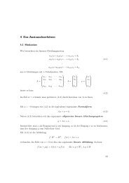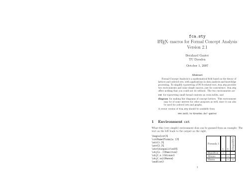
fca.sty LATEX–macros for Formal Concept Analysis Version 2.1

fca.sty
L ATEX–macros for Formal Concept Analysis
Version 2.1
Bernhard Ganter
TU Dresden
October 1, 2007
Abstract
Formal Concept Analysis is a mathematical field based on the theory of
lattices and ordered sets, with applications in data analysis and knowledge
processing. To simplify typesetting of FCA-related text, fca.sty provides
two environments and some simple macros, just for convenience. fca.sty
offers nothing that you could not do without. The two environments are
cxt for typesetting small formal contexts as cross-tables, and
diagram for making line diagrams of concept lattices. This environment
may be of some interest for other purposes as well, since it can also
be used for ordered sets and graphs.
A recent version of fca.sty should be available from
1 Environment cxt
www.math.tu-dresden.de/∼ganter
What this (very simple) environment does can be guessed from an example: The
text on the left leads to the output on the right.
\begin{cxt}%
\cxtName{Formula 1}%
\att{1.}%
\att{2.}%
\atr{disqualified}%
\obj{x..}{Hamilton}
\obj{.x.}{Alonso}
\obj{.xx}{Massa}
\end{cxt}
1
disqualified
Formula 1
1. 2.
Hamilton ×
Alonso ×
Massa × ×

cxt generates a tabular of the appropriate format. The tabular is defined as
soon as the first \obj command is given. Spaces in the preceding lines are not
ignored (in this version). Therefore, each line should be ended with a % . (To be
repaired in later versions).
The commands within a cxt–environment are
\cxtName{} Define the text for the upper left cell of the table. Optional. The
default is no text.
\att{} Give an attribute name. These names are processed in the order in
which they are given. Attribute names given after an \obj command are
ignored.
\atr{} Same as \att{}, but with rotated text.
\obj{}{} Give an object’s name and its incidence vector, consisting of dots
and ‘x’es. The incidences come first, for better alignment. The length of
each incidence vector must be the number of attributes.
Each instance of \obj is directly translated to a row of the tabularenvironment.
It is therefore possible to mix \obj commands with usual
tabular-commands.
cxt can handle up to 20 attributes.
The arrow relations may also be used. Instead of x and ., type d (for “down”),
u (“up”), or b (“both”), as in the following example:
\begin{cxt}%
\renewcommand{\cxtArrowStyle}{\footnotesize\color{red}}
\cxtName{Formula 1}%
\att{1.}%
\att{2.}%
\atr{disqualified}%
\obj{xbd}{Hamilton}
\obj{uxb}{Alonso}
\obj{bxx}{Massa}
\end{cxt}
Formula 1
1. 2. disqualified
Hamilton × ↗↙ ↙
Alonso ↗ × ↗↙
Massa ↗↙ × ×
The default for \cxtArrowStyle is \footnotesize. In the above example
we have changed it using \renewcommand in order to make the arrows red. The
default colour is black.
2

\IUpArrow Gives ↖, which is has the same meaning as ↗, but is drawn in
the other direction. This is needed in the definition of ↙.
\IHochpfeil Same as \IUpArrow.
\DDArrow Gives ↙, the symbol for the transitive closure of the arrow relations.
\DDPfeil Same as \DDArrow.
\NDDArrow Gives ↙\ the symbol for the negation of ↙.
\NDDPfeil Same as \NDDArrow.
\Semi Gives � � , the symbol for the semi-product.
\FCA Prints “Formal Concept Analysis”. In most cases, this command does
not eat the space following it (thanks to \xspace).
\FBA, \FnBA Print “Formale(n) Begriffsanalyse”. These commands also use
\xspace so that blanks are preserved.
Some symbols that are provided by L ATEX are listed in Figure 2.
Here is a sample text:
\FCA offers an elegant way to determine the congruence relations
of a complete lattice: The congruence lattice of a doubly founded
concept lattice $\CLGMI$ is isomorphic to $\CL(G,M,\NDDArrow)$.
This translates to:
Formal Concept Analysis offers an elegant way to determine the congruence
relations of a complete lattice: The congruence lattice of a doubly
founded concept lattice B(G, M, I) is isomorphic to B(G, M, ↙\ ).
4 To do
• Improve the placement of the dotted lines connecting nodes with attributeand
object names.
• Allow half-shaded nodes in diagrams, and make them (optionally) automatic
for object- and attribute concepts.
• Improve the code to avoid unwanted blanks.
10
2 Environment diagram
The diagram environment helps typesetting diagrams of concept lattices, but can
be used for ordered sets and graphs as well. Again we start with a small example
(for which we have set \unitlength 1.2mm):
\begin{diagram}{40}{55}
\Node{1}{20}{10}
\Node{2}{35}{20}
\Node{3}{5}{30}
\Node{4}{35}{40}
\Node{5}{20}{50}
\Edge{1}{2}
\Edge{1}{3}
\Edge{2}{4}
1.
\Edge{3}{5}
Hamilton
\Edge{4}{5}
%\Numbers
\leftAttbox{3}{2}{2}{1.}
\rightAttbox{2}{2}{2}{disqualified}
\rightAttbox{4}{2}{2}{2.}
\leftObjbox{3}{2}{2}{Hamilton}
\rightObjbox{2}{2}{2}{Massa}
\rightObjbox{4}{2}{2}{Alonso}
\end{diagram}
Here are the commands of the diagram–environment:
\begin{diagram}{width}{height} translates to
2.
Alonso
disqualified
Massa
\begin{picture}(width,height)(\diagramXoffset,\diagramYoffset).
The offsets are zero by default. They can be modified using \renewcommand.
Note that the diagram dimensions do not take the lables into account, these
may overlap. Putting an \fbox around the above diagram yields (with
\unitlength .7mm)
1.
Hamilton
3
2.
Alonso
disqualified
Massa

\Node{nodenumber}{xpos}{ypos} Puts a circle at position (xpos,ypos) of
the picture. These circles are drawn when \end{diagram} is invoked. The
default diameter of the circles is 4 (times \unitlength). It can be changed
(for all circles) with \CircleSize{}. The argument must be an integer.
The node numbers must be different, consecutive between 0 and 51, but
need not necessarily be given in ascending order.
\Numbers Puts numbers inside circles. While working on a diagram it can be
helpful to have a picture with numbered nodes. The result of the following
command sequence is shown on the right:
\fbox{\unitlength .7mm
\begin{diagram}{40}{55}
7
\Node{5}{20}{10}
8
\Node{6}{35}{20}
4
\Node{4}{5}{30}
\Node{8}{35}{40}
6
\Node{7}{20}{50}
5
\Numbers
\end{diagram}}
We recommend to remove the \Numbers–command when the diagram is
ready. In most cases it is not a good idea to put text inside the nodes of a
diagram.
\Edge{nodenumber1}{nodenumber2} Puts a line between the two nodes with
the given numbers. These must have been declared earlier with a \Node–
command. For nodes with coordinates (u,v) and (x,y) the command
translates to
\fcadrawline(u,v)(x,y).
\fcadrawline(u,v)(x,y) is a pdfL ATEX–compatible reimplementation of
the \drawline command, the latter provided by the eepic package.
The \Edge–command is executed immediately. It can be mixed with other
picture- and eepic–commands like \spline. Line thickness can be set
with \thicklines, \Thicklines, \thinlines, and \allinethickness{}
(see the eepic manual).
\leftAttbox{nodenumber}{xoffset}{yoffset}{text1\\ text2\\ ...}
This is one of six commands
{\left, \center, \right}×{Attbox, Objbox}.
4
Result command German version
(G, M, I) \GMI
K \context
L \context[L]
B \CL \BV
B(G, M, I) \CLGMI \BVGMI
B(G, M, I) \CGMI \BGMI
ext() \extent{}
int() \intent{}
Ext() \extents{}
Int() \intents{}
(H, N, I ∩ H×N) \HNI
I \relI
̷I̷
× �
�
\notI
\bigtimes
\Semi
↙ \DownArrow \Runterpfeil
↗ \UpArrow \Hochpfeil
↗↙ \DoubleArrow \Doppelpfeil
↖ \IUpArrow \IHochpfeil
↙ \DDArrow \DDPfeil
↙\ \NDDArrow \NDDPfeil
Formal Concept Analysis \FCA
Formale Begriffsanalyse \FBA
Formalen Begriffsanalyse \FnBA
Figure 1: Table of fca.sty–macros.
Symbol command package required
∨ \vee
∧
�
\wedge
�
\bigvee
⊔
\bigwedge
\sqcup
⊓
�
�
\sqcap
\bigsqcup
\bigsqcap stmaryrd
Figure 2: Other symbols that are used in Formal Concept Analysis, and the
commands that generate them.
9

3 Some macros
For a short description see Figure 1.
\GMI The formal context (G, M, I).
\context The symbol K, a frequently used name for a formal context.
\context[S] Other letters, such as S, may also be used.
\CL The symbol B for the concept lattice operator. If K is a formal context,
then B(K) denotes its concept lattice.
\BV same as \CL.
\CLGMI The concept lattice B(G, M, I) of the formal context (G, M, I).
\BVGMI Same as \CLGMI.
\CGMI The set B(G, M, I) of all formal concepts of the formal context (G, M, I).
\BGMI Same as \CGMI.
\extent The extent ext(c) of the formal concept c := (A, B) is A.
\intent The intent int(c) of the formal concept c := (A, B) is B.
\extents The set Ext(K) of extents of the formal context K.
\intents The set Int(K) of intents of the formal context K.
\HNI The subcontext (H, N, I ∩ H×N).
\relI The incidence relation I.
\notI The negation ̷I̷ of the incidence relation.
\bigtimes The product symbol ×.
\DownArrow The ↙ of the arrow relations.
\Runterpfeil Same as \DownArrow.
\UpArrow The ↗ of the arrow relations.
\Hochpfeil Same as \UpArrow.
\DoubleArrow The ↗↙ of the arrow relations.
\Doppelpfeil Same as \DoubleArrow.
8
These are used to put text to diagram nodes. The Attbox–commands place
the text above the corresponding node, the Objbox below. Similarly, the
text can be placed to the left, be centered, or be placed to the right of
the labelled node. All this can be modified with the xoffset, yoffset–
parameters.
The offsets increase the placement effect. A \rightObjbox, which is placed
to the lower right of the corresponding node, will be moved even further
to the lower right if the offsets are positive. Similarly, positive offsets will
push a \leftAttbox even more to the upper left, etc.
The text of the label is put in a \parbox. It can be broken into several
lines using \\. The width of the \parbox is \LabelBoxWidth, with a default
value of 40mm. This can be changed using \renewcommand.
The label text and the labelled node are connected with a dotted line. Here
is an example:
{\unitlength .7mm
\begin{diagram}{40}{15}
\Node{0}{20}{10}
\leftAttbox{0}{1}{1}{left\\
attribute\\ label}
\rightAttbox{0}{10}{10}{right
attri-\\ bute label}
\rightObjbox{0}{20}{5}{right\\
object\\ label}
\centerObjbox{0}{0}{5}{centered\\
object label}
\end{diagram}}
The style of the lables is given by
left
attribute
label
centered
object label
\ObjectLabelStyle Default: \small\baselineskip6pt\rm
right attribute
label
\AttributeLabelStyle Default: \small\baselineskip6pt\it.
These values can be changed with \renewcommand.
right
object
label
\end{diagram} This concludes the diagram. The circles representing the
nodes are drawn and filled with white. Everything inside such a circle
(except for the numbers caused by the \Numbers command) is erased.
2.1 Error messages
Package error messages for the diagram environment are not yet implemented.
Errors usually are caused by using node numbers that have not been defined
earlier.
5

2.2 Fine tuning
You can change certain layout parameters either permanently (by modifying the
file fca.sty) or temporarily using the following commands:
\CircleSize{}, Default: 4 (times \unitlength)
\NodeColor{}, Default: white
\NodeThickness{}, Default: 1.2pt
\EdgeThickness{}, Default: .8pt
\NoDots,
\renewcommand{\ObjectLabelStyle}{},
\renewcommand{\AttributeLabelStyle}{},
\renewcommand{\LabelBoxWidth}{}.
Except for the first three, these commands can be focussed to single instances,
using brackets. For example,
{\NoDots\centerObjbox{nodenumber}{xoffset}{yoffset}{labeltext}}
generates a single centered object label without dotted line.
2.3 pdfL ATEX compatibility
Version 2 of the diagram environment was designed to be pdfL ATEX compatibile.
It no longer uses eepic.sty, which is not supported by pdfL ATEX. Instead it uses
pict2e and a \fcadrawline command, that replaces eepic’s \drawline.
2.4 Problems with colour
Since the diagrams are drawn using the picture–commands and the pict2e
package, we can combine with other packages, for example, with the color package.
This allows us to colour edges and text (but not individual nodes, see 2.5).
However, color has a problem with spacing. Changing colors can cause unwanted
spaces, and these are particularly unpleasant in pictures. Have a look at
the following:
{\unitlength 2mm
\begin{diagram}{20}{20}
\Node{1}{5}{5}
\Node{2}{15}{15}
{\color{red}\Edge{1}{2}}
{\color{blue}\Edge{1}{2}}
{\color{red}\Edge{1}{2}}
{\color{blue}\Edge{1}{2}}
\end{diagram}}
6
This effect disappears when spaces are avoided. Here is a better version:
{\unitlength 2mm
\begin{diagram}{20}{20}
\Node{1}{5}{5}
\Node{2}{15}{15}
{\color{red}\Edge{1}{2}}%
{\color{blue}\Edge{1}{2}}%
{\color{red}\Edge{1}{2}}%
\color{blue}\Edge{1}{2}}%
\end{diagram}
2.5 Colouring nodes
Nodes are filled with white by default. This can be changed to any other colour
using the command \NodeColor{colorname}. This color then applies to all
nodes. colorname must be a color specification as used by the color package.
‘‘red’’, ‘‘blue’’, and ‘‘green’’ should usually work. Other colors may be defined
with the \definecolor command, see the documentation of the graphics
bundle. For finer colour nuances use the xcolor package and its documentation.
fca.sty does not support individual node colouring, but there is a trick to
do it nevertheless. Simply include the diagram environment into a picture
environment and insert the coloured nodes after the diagram is drawn. How
this is done should become clear from the example below. fca.sty provides a
command \ColorNode{colorname} for this. It overwrites numbers generated by
the \Numbers command.
{\definecolor{grey}{gray}{.8}
\unitlength 2mm
\NodeThickness{2.5pt}
\EdgeThickness{2.5pt}
\begin{picture}(20,20)%
\put(0,0){%
\begin{diagram}{20}{20}
\NodeColor{grey}
\Node{1}{5}{5}
\Node{2}{15}{15}
\Edge{1}{2}%
\end{diagram}}
\put(5,5){\ColorNode{green}}
\end{picture}}
7