mm$m> - Department of Mathematics - Harvard University

Website. Further information about The HCMR can be
found online at the journal's website.
http://www.thehcmr.org/
Instructions for Authors. All submissions should in
clude the name(s) of the author(s), institutional affiliations (if
any), and both postal and e-mail addresses at which the cor
responding author may be reached. General questions should
be addressed to Editor-in-Chief Rediet Abebe at hcmrjhcs.
harvard. edu.
Articles. The Harvard College Mathematics Review invites
the submission of quality expository articles from undergrad
uate students. Articles may highlight any topic in undergrad
uate mathematics or in related fields, including computer sci
ence, physics, applied mathematics, statistics, and mathemat
ical economics.
Authors may submit articles electronically, in .pdf, ps,
or .dvi format, to hcmr3hcs.harvard.edu, or in hard
copy to
The Harvard College Mathematics Review
Student Organization Center at Hilles
Box # 360
59 Shepard Street
Cambridge, MA 02138.
Submissions should include an abstract and reference list. Fig
ures, if used, must be of publication quality, lf a paper is
accepted, high-resolution scans of hand drawn figures and/or
scalable digital images (in a format such as .eps) will be re
quired.
Problems. The HCMR welcomes submissions of original
problems in all mathematical fields, as well as solutions to
previously proposed problems.
Proposers should send problem submissions to Problems
Editor Yale Fan at hcmr-problems@hcs . harvard. edu
or to the address above. A complete solution or a detailed
sketch of the solution should be included, if known.
Solutions should be sent to hcmr- solutions@hcs.
harvard.edu or to the address above. Solutions should
include the problem reference number. All correct solutions
will be acknowledged in future issues, and the most outstand
ing solutions received will be published.
Advertising. Print, online, and classified advertisements
are available; detailed information regarding rates can be
found on The HCMR's website, (1). Advertising inquiries
should be directed to hcmr-advert iseghcs. harvard,
edu, addressed to Business Manager Hamsa Sridhar.
Subscriptions. One-year (two issue) subscriptions are
available, at rates of $5.00 for students, $7.50 for other indi
viduals, and $15.00 for institutions. Subscribers should mail
checks for the appropriate amount to The HCMR's postal ad
dress; confirmation e-mails or queries should be directed to
hcmr-subscribe@hcs.harvard.edu.
(1)
Sponsorship. Sponsoring The HCMR supports the un
dergraduate mathematics community and provides valuable
high-level education to undergraduates in the field. Sponsors
will be listed in the print edition of The HCMR and on a spe
cial page on the The HCMR's website, (1). Sponsorship is
available at the following levels:
partment
Sponsor $0 - $99
Fellow $100-$249
Friend $250 - $499
Contributor $500 $1,999
Donor $2,000 - $4,999
Patron $5,000 - $9,999
Benefactor $10,000 +
Contributors • The Harvard University Mathematics De
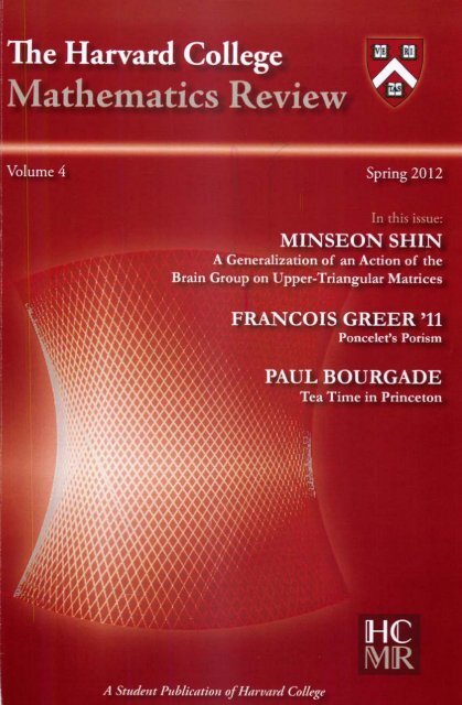
Cover Image. The image on the cover depicts an integral
billiard (ellipse). This issue's article "Tea Time in Princeton"
by Dr. Paul Bourgade (p. 41) discusses eigenvalues of random
matrices and their connection to number theory.
©2007-2012 The Harvard College Mathematics Review
Harvard College
Cambridge. MA 02138
The Harvard College Mathematics Review is produced and
edited by a student organization of Harvard College.

— -2 —
Contents
0 From the Editors
Rediet Abebe and Greg Yang, Harvard University '13 and '14 3
Student Articles
1 A Generalization of an Action of the Braid Group on Upper-Triangular Matrices
M i n s e o n S h i n , M a s s a c h u s e t t s I n s t i t u t e o f Te c h n o l o g y ' 1 3 4
2 Modular Forms for the Congruence Subgroup T(2)
G r e g Y a n g , H a r v a r d U n i v e r s i t y ' 1 4 1 7
3 The 5 Function as a Measure
T h o m a s M e y e r , C o l u m b i a U n i v e r s i t y ' 1 3 2 7
4 Widths in Graphs
Anand Oza and Shravas Rao, Massachusetts Institute of Technology '14 and '13 32
Faculty Feature Article
5 Tea Time in Princeton
P r o f . P a u l B o u r g a d e , H a r v a r d U n i v e r s i t y 4 1
Features
6 Mathematical Minutiae • Four Proofs of the Integer Side Theorem
E v a n O ' D o r n e y , H a r v a r d U n i v e r s i t y ' 1 5 5 4
7 Applied Mathematics Corner • Minimum Variance Inflation Hedge
A d a m A r t h u r s , H a r v a r d U n i v e r s i t y ' 1 2 5 8
8 My Favorite Problem • Poncelet's Porism
F r a n c o i s G r e e r , H a r v a r d U n i v e r s i t y ' 1 1 7 2
9 P r o b l e m s 77
1 0 S o l u t i o n s 79
11 Endpaper • Waiting for Mathematics
P r o f . G e r a l d E . S a c k s , H a r v a r d U n i v e r s i t y 8 1

Editors-In-Chief
Rediet Abebe ' 13 and Greg Yang ' 14
A r t i c l e s E d i t o r F e a t u r e s E d i t o r
G e o f f r e y L e e ' 1 4 L u c i a M o c z ' 1 3
P r o b l e m s E d i t o r B u s i n e s s M a n a g e r
Y a l e F a n ' 1 4 H a m s a S r i d h a r ' 1 2
Issue Production Director
Eric Larson '13
Graphic Artist
KeoniCorrea '13
Editors Emeritus
Zachary Abel' 10, Ernest Fontes ' 10, Scott Kominers '09/AM' 10/PhD' 11
Webmasters
Rediet Abebe ' 13 and Akhil Mathew ' 14
Board of Reviewers
Rediet Abebe.'13
Levent Alpoge ' 14
JohnCasale'12
Irving Dai' 14
Yale Fan'14
Marco Gentili '15
Eric Larson '13
Geoffrey Lee '14
Akhil Mathew '14
Lucia Mocz '13
SethNeel'15
ToanPhan'14
Caitlin Stanton '14
Allen Yuan '15
Faculty Adviser
Professor Peter Kronheimer, Harvard University

o
From the Editors
Rediet Abebe
Harvard University ' 13
Cambridge, MA 02138
rtesfaye@college.harvard.edu
Greg Yang
Harvard University ' 14
Cambridge, MA 02138
gyang@college.harvard.edu
Many of us have grown up with math books and math competitions. We remember the adrena
line rush as the clock ticked down on the tests and the sleepless nights spent on attacking problems
and deciphering theories. We still maintain the friendships that are made through the common
interest of mathematics. That part of our childhoods have long been ingrained into our characters,
and we inherit these symptoms of love for mathematics even in college.
Now we, the HCMR staff, have the honor to celebrate this love by furnishing the texts that
would hopefully become the material of somebody's sleepless nights. For this process, we have
had the fortune of many people's support. The two of us would like to thank the HCMR staff and
executive members for the endless enthusiasm and dedication to the making of this journal. It has
been a privilege to work with such committed members over the past year. The HCMR could not
have grown to the level of visibility across departments around the nation and the world without
your contribution.
As always, we owe our deepest gratitude to members of the Harvard College Math Depart
ment for the advice, encouragement and guidance throughout the publication process. We would
like to thank the HCMR's advisors and sponsors for the profound contributions which continue
to make this journal a success; and the Student Organization Center at Hilles for providing the
HCMR a space in which to grow.
Finally, we would like to thank our readers for all the input you have given us in person and
via email. Please feel free to continue to contact us with any comments, questions and concerns
you may have.
This issue marks the fourth volume since the inception of the Harvard College Math Review
and the second since it became an annual publication. Over the five years that the HCMR has stood
as a student-run organization, it has had celebration of mathematics both in its pure and applied
form at the heart of its mission. We hope you find joy in such a celebration as we did in creating
this journal.
Rediet Abebe ' 13 and Greg Yang ' 14
Editors-In-Chief, The HCMR

STUDENT ARTICLE
1
A'Generalization of an Action of the
Braid Group on Upper-Triangular
Matrices
Abstract
Minseon Shin*
Massachusetts Institute of Technology ' 13
Cambridge, MA 02138
mshin@mit.edu
We investigate various questions related to a conjecture posed by A. I. Bondal in his 2004 paper "A
symplectic groupoid of triangular bilinear forms." Bondal describes an action of the braid group
of n strings B„ on the n x n upper-triangular matrices, which has a natural (linear) algebraic
formulation obtained by embedding Bn into a group of matrices whose entries are polynomials
in n^n~l) indeterminates (with an unusual composition law). One can try to extend the action to
other matrices in this group to get a larger group acting on the set of upper-triangular matrices.
Bondal conjectures that the action cannot enlarge past Im(B„ tx (Z/2Z)n). In this paper, we
prove Bondal's conjecture for the case n = 2, study the elements that act trivially, and present an
unfinished inductive strategy for proving the conjecture for n > 3.
1.1 Introduction
Let k be an algebraically closed field of characteristic zero, let V be a vector space of dimension n
over k, and let ( , ) be a nondegenerate bilinear form on V. Let E be the set of ordered bases of V.
Definition 1. An ordered basis E = (ei,..., en) is called semiorthogonal if {a, ej) = 0 for all
i > j and (e^ ei) = 1 for all i.
Let Es C E be the set of ordered semiorthogonal bases of V and consider the group Perm(Es)
of permutations of Es. Bondal proved in [1] that Perm(Es) contains a subgroup isomorphic to the
braid group, which is defined as follows.
Definition 2. The braid group Bn has generators {a\,..., an- i } with relations
O i G j = G j G i i f \ i - j \ > 1
G i G i + i G i = ( J i + i O i G i + i f o r 1 < i < n — 2 .
Definition 3. For i = 1,..., n - 1, define the transformation pi '- E -» E which maps the ordered
basis E = (ei,...,e„) to ipi{E) = {e\,.. .,e'n) where
e'i = ei+i-(ei,ei+i)ei
i
ei+l — ei
e'j — ej for j 0 {i,i + 1} .
^Minseon Shin, Massachusetts Institute of Technology ' 13, is a mathematics major. His current mathemati
cal interests include algebra and combinatorics. Outside of academics, he enjoys listening to music and playing
soccer.

Minseon Shin—Action of the Braid Group on Upper-Triangular Matrices 5
It is easily checked that if E is semiorthogonal, then fi(E) is semiorthogonal. Therefore fi
permutes the set of semiorthogonal bases: fi G Perm(E.s). The transformation fi, when restricted
to Es, has an inverse^"1 : Es ->- Es which maps E = (ei,... ,en) to v?"1^) = (ei,. . .,e'n)
where
ei = ei+i
ei+1 = ei — (ei,ei+i)ei+i
e'j =ejforj 0 {2,2 +1} .
Proposition 4 (Bondal [1] 2.1). 77*e correspondence ai 1—▶ (fi can be extended to an action of
the braid group by automorphisms on the set of semiorthogonal bases.
In other words, the correspondence en \—> (fi can be extended to a homomorphism Bn -»
Perm(Es). As Bondal notes, this action of Bn on Es is not faithful, because the center Z(Bn) acts
trivially on Es (we prove this fact in Section 1.4). However, it is possible to embed this group in a
particular group of matrices with a special law of composition.
The matrix of the bilinear form with respect to a semiorthogonal basis is upper-triangular with
ones on the main diagonal; the space of such upper-triangular matrices with ones on the main
diagonal constitutes an affine space of dimension n^n~^, which we denote by A.
Let R be a ring, let X = {Xij : 1 < i < j < n} be a set of nis^ll ^determinates, let R[X]
be the polynomial ring over the indeterminates X and coefficients in R, and let Mn(X, R) be the
set ofnxn matrices whose entries are in R[X], Let X be the n x n upper-triangular matrix with
ones on the main diagonal and whose {i, j)th entry is Xij for all i < j. For any B G Mn(X, k)
and A G A we denote by BA or B{A) the matrix obtained by evaluating B at A; specifically,
substituting Aij -» Xij.
Let us associate, to each generator cr* of the braid group Bn, a matrix &i{X) G Mn(X, k)
which coincides with the identity matrix In at all entries except for the 2 x 2 matrix
0 1
1 X i , i + \
which is situated so that Xi,t+i is the {i + 1, i + l)th entry of a(X). If n
have
1
*i(*)
^12 and CT2(X) = 1
1
1
-^23
3, for example, we
The motivation for this definition is the following property of semiorthogonal bases. For every
E G Es, let AE be the matrix of the form ( , ) with respect to E. Then AE is upper-triangular and
o-i(A-E) is the change-of-basis matrix from fi{E) to E\ in other words, the matrix which satisfies
E = ipi(E)

6 T h e H a r v a r d C o l l e g e M a t h e m a t i c s R e v i e w 4
Definition 6. Bo(n) is a monoid with the composition law * defined as follows: For B,C G Bo(n),
let
B * C = B c - t x c - i C x . ( 1 . 2 )
This law of composition * is well-defined, associative, and has an identity which is simply the
identity matrix / (these properties may be verified easily).
Definition 7. Let us denote by B{n) C Bo{n) the set of elements in Bo(n) which have two-sided
inverses with respect to *.
Then cn(A) G B(n) for all i, where the inverse of a*(A) with respect to * is a~l(A). (In
general, a~x (A) is not equal to (cri(A))-1, the inverse of cn(A) with respect to matrix multiplica
tion.) There are other elements of Mn (X, k) that, trivially, lie in B{n). For every s = (si,..., sn) G
(Z/2Z)n, define the diagonal matrix Ns whose (i,i)th entry is (-l)s\ which represents the ba
sis transformation (ei,... ,en) i—> ((-l)siei,..., (-l)5nen). Then Ns lies in B{n), and its
inverse with respect to * is itself.
Definition 8. There is a natural action • : B{n) x A -> A of B{n) on A, defined as follows:
B - A = B a T A B a 1 . ( 1 . 3 )
Proposition 9 (Bondal [1] pg. 669). Consider the semidirect product Bn tx (Z/2Z)n; the Junction
f : B n x ( Z / 2 Z ) n - > B { n ) ( 1 . 4 )
mapping a \—> ai(A)forai G Bn and s i—▶ iVs/or s G (Z/2Z)n w fl monomorphism.
We are primarily concerned with the following conjecture posed by Bondal:
Conjecture 10 (Bondal [1] 2.2). The monomorphism f defined in Proposition 9 is also surjective.
Bondal stated that he knew the proof for the cases n < 3. While we do not prove the conjecture
in its entirety, we describe and prove a number of small related results.
Structure of paper. In Section 1.2, we state and prove some basic constraints on an element B
of B{n). In Section 1.3, we prove Conjecture 10 for the case n = 2. In Section 1.4, we study
elements of B(n) acting trivially on A. In (1.4.1), we explicitly compute the matrix associated
to the generator of the center of Bn. Though we cannot prove that this generates, up to signs,
the group of elements in B{n) acting trivially, we prove some lemmas toward this (1.4.2). In
Section 1.5, we present an inductive strategy for proving Conjecture 10 for higher values of n; we
do not fulfill this agenda, but set up some of the steps.
Sections 1.3,1.4, and 1.5 each require the reader to have read only Sections 1.1 and 1.2. Person
ally, I feel the most interesting results and conjectures are Lemma 18, Conjecture 20, the discussion
in Section 1.4.1, and Proposition 44.
Acknowledgements. This work was undertaken as part of the Summer Program for Undergraduate
Research run by the MIT math department over summer 2011.1 would like to thank the MIT math
department for supporting me, Professor David Jerison for organizing SPUR, Professor Paul Seidel
for suggesting the problem, and my mentor Ailsa Keating for her mathematical insights and advice,
as well as her extensive help on editing and formatting this paper.
1.2 Basic Constraints
1.2.1 Coordinate-free constraints
Lemma 11 and its Corollary 12 show that if B G Bo{n) then the entries of B~l are actually ele
ments of k[X], instead of rational functions in k(X), as originally defined in Definition 5. Propo
sition 13 is stated without proof since it not used elsewhere in this paper; however, it may provide
the reader with intuition on the structure of Bo{n).

Minseon Shin—Action of the Braid Group on Upper-Triangular Matrices 7
Lemma 11. Suppose that B G Bo(n). Then det B = ±1.
Proof If Be B0(n), then A! = B~AT AB~Al G A for all AeA. Since det A = 1 for all AeA,
we have (det BA)~2 = det{BATABAl) = det A' = 1 which implies det BA = ±1. Since BA
depends continuously on A, so does det BA, so det B — +1 (or —1) identically. D
Corollary 12. Suppose that B G Bo{n). Then B~x has polynomial entries. □
Proposition 13. (a) //"£? G #o(n), f/iew Pj is orthogonal. Moreover, B I = I.
(b) IfBe f(Bn), then Bi is a permutation matrix.
(c) IfBe Bo(n) n Mn(X, Z), then B\ is a permutation matrix (up to signs).
(d) IfB e Imp, then B e Mn(X,Z).
1.2.2 A Symmetric Polynomial Equation
Suppose that B e B{n)\ we investigate a polynomial equation satisfied by the coordinates of each
column of B~x. Definition 14 is motivated by Lemma 15.
Definition 14. For any f := (/i,..., fn) e (k[X])n and any nonempty S c [n], define
t G S i , j € S,i (k[X])n which maps
(/i,...,/„) to (/{,...,/A) where
f'_J-/i if* 7^
Lemma 17. For ««>' £, f/*e composition Te o 7> /s f/*e identity. □

8 T h e H a r v a r d C o l l e g e M a t h e m a t i c s R e v i e w 4
Lemma 18. For any £, the transformation Te preserves the quantity P[n] (f). In other words,
F[n](lKf)) = P[n](f).
Proof. We prove the lemma for £ — n; the proof is analogous for £ = 1,..., n — 1. Let f :—
(/!,...,/„) and f':=7i(f) = (/{,...,/A). Then
P[n](?) = Pt„-i](f') + fnl In + £ X,n/;
= i^„-l](f)+(/n + X)^„/iJ/„
= ^ t n ] ( f ) □
Let Y = {Vi : 1 < i < m) be another set of indeterminates. In Lemma 19 and Conjec
ture 20, we consider the fi to be elements in k[X, Y] instead of in k[X] in the hope that it will help
in an inductive solution, for example in Proposition 44.
Lemma 19. Suppose that f = (/i,... ,/„) G {k[X, Y])n satisfies P[n](f) = 0 or 1. Lef ofc to?
the (total) degree of f% and let d = ma,Xi{di} and suppose that d > 1. If there is exactly one £
such that de = d, then Te reduces the degree offe.
Proof. Let de = d. The condition that there is exactly one £ such that de = d implies that di < de
if i ^ £. If di < de -1 for all i ^ £, then ff has the unique highest degree in P[n] (f), contradiction.
Thus there exists some i such that di = de -1. Let S be the set of all indices i such that di — dt — \.
Let gi e kjX, Y] be the "leading term" of /i, the sum of monomials of maximal total degree in
fi. Then g\ + £iG5 A^tf* = 0. But ge + J2ies X^9i is the leading term of the £th term of
Ti(f). □
Conjecture 20. A// f/ie solutions to P[n] (f) = lfor fi,... ,fn G /c[X, Y] aw te reduced by the
transformations Te to one of the "elementary solutions", in which all but one fz are zero and the
nonzero fi is either ±1. More precisely, for any solution f to P[n] (f) = 1, there exists a finite
sequence a\,..., aN G [n] such that Tai (• • • (TaN (/))•••) is an elementary solution.
1.3 The case n = 2
We give a full proof of Conjecture 10 for the case n = 2. We use coordinates, so the lemmas given
here depend heavily on the the fact that n = 2. We have not been able to generalize most of them
to higher dimensions.
We will use the notation:
where btj G k[x\. Let fi := det B. Then
"1 -
X'1 =
1
*l(X) =
1
and Bx
bn
621
1
1 X M*))_1 =
b\2
622
- x 1
1
We start with two technical lemmas that will get used in the proof the theorem.
\X)-
X 1
1
Lemma 21. Let B e M2(X, k); then B e Bo{2) if and only if the entries bij satisfy the following
conditions:
^21 + £>22 ~ Xb2lb22 = 1
&11 +b?2 -xbiibn = 1
xb\2b2i — 611621 — 612622 = 0
(1.5)
(1.6)
(1.7)

Minseon Shin—Action of the Braid Group on Upper-Triangular Matrices 9
Proof This is immediate from
B y X B y =
Lemma 22. IfBe B0{2), then
(a) B-/XBX1 =
(b)
622 621
612 6n
(cj 621 = -^612.
621 + 622 — ^621622 ^611622 — 611621 — 612622
^612621 - 611621 - 612622 6f! + 612 - ^611612
1 p x
1
G B0(2).
M 622 =P{-xbi2 + 611).
(e) Suppose that bij ^ Ofor all i, j and let dij = deg bij. Then there exists a positive integer
m such that one of the following holds:
{dn = ra — 1 , du = cbi = ra , c?22 = m + 1}
{dn =m+l , di2 = cfei = ra , 0^22 = m — 1}.
/V00/ Each of these properties follows from manipulating the conditions of Lemma 21; we omit
the proofs. □
We are now ready for the proof of Conjecture 10 for n = 2. We proceed in two steps.
Lemma 23. Bo{2) = B{2). Given B e Bo{2), an explicit inverse with respect to * is C given by:
C
if det B = 1
if det B = -1
Proof. Suppose B e B0{2) and det B = -1; the case det B = 1 is similar, and we omit it. Then
BjfXBx1 = X-1 if and only if B^X^Bx = X. Let C := p-^thenC G M2(X,fc) and
CX = B^_1XBx-i = X~l eAsoCe B0(2). It suffices now to show that P*C = C*P =
L Since CX = X~\ we have B*C = BCxCx = Bx-iCx = L Also, BX = X~l so
C * B = C b x B x = C x - i B x = / . D
Theorem 24. Every B G B(2) w contained in the image ofB2 X (Z/2Z)2.
Proof We proceed case by case. Suppose 612 = 0 then, by Lemma 22(c), 621 = 0. By Lemma 21
(1.5,1.6), 61! = 622 = 1. This gives us the four matrices [Vii]' which is exactly the image of
(Z/2Z)2.
Suppose that 612,621 ^ 0. If bn = 0, then (1.6) implies that 612 = ±1. So 621 = ±1
by Lemma 22(c). Now (1.7) implies that 622 = 621^; this is equal to the image of

10 The Harvard College Mathematics Review 4
1.4 Trivial actions and the center of the braid group
1.4.1 A proof that f> {{oxo2 • • • on-x)n) = X~TX
The center of the braid group Bn is cyclic with generator (eri

Minseon Shin—Action of the Braid Group on Upper-Triangular Matrices 11
Proof Let Eij be the nxn matrix which differs from the zero matrix by a 1 in its (i, j)th entry.
Then Ei1j1Ej2i2 = Ej2i2Ei1j1 = 0 since j\ ^ J2 and i\ ^ z-2. Thus we have
--T
LhhLi'
{I Xilj1Ej1i1)(I -h Xi2j2Ei2j2) — I Xi1j1Ej1i1 + Xi2j2Ei2
-ki2J2^iiji ~~ (-* + Xi2j2Ei2j2){I Xi1j1Ejli1) — I + Xi2j2Ei2j2 — Xi1j1Ej1i1 ,
hence LiljlLi2j2 = Li2j2Liiji.
Lemma 31. IfB = (f(sn), then
B =
In-l
1 x1
Example 32. For the case n — 3 we have
and B • X
X -xl
1 "l X23
— X12
&2cr\)x =
1 X12
1
Xl3.
f((T20-l) • X = 1 — X13
1
Proof of Lemma 31. We prove by induction that f{am • • • 0"i) transforms the basis
where
E = (ei,...,e„) -> E' = (ex,...,en),
6j = ei+i - (ei,ei+i)ei for z = 1,... ,ra,
e^+1 = ei, and
e ■ = ei for i > ra + 1 .
The base case ra = 1 is immediate. For general ra, the basis E' — {e\,..., e'n) under the
transformation

1 2 T h e H a r v a r d C o l l e g e M a t h e m a t i c s R e v i e w 4
Example 34. The case n = 3. We have already computed f{(72

Minseon Shin—Action of the Braid Group on Upper-Triangular Matrices 13
Equality 1 follows from the definition of the law of composition *; equality 2 follows from the fact
thatPi+1Pn_1_i = JforalH = 1,... ,n-1; equality 3 follows directly from Lemma 35; equal
ity 4 follows from rearranging the Ltj and L~T according the commutativity rules in Lemma 30;
f i n a l l y , e q u a l i t y 5 f o l l o w s d i r e c t l y f r o m L e m m a 2 8 . □
1.4.2 Regarding the converse
We now explore the converse: if P G B{n) and that P acts trivially on A, then is it true that P is
contained in the image of the center of Pn, i.e., Bx = (X~TX)k for some k G Z?
To show BA = (A~TA)n for all A e A it is enough for it to be true in some nonempty open
subset of the affine space A.
Lemma38. IfB e B(n)andBATAB'1 = AforallA e A, thenBx(X~TX) = {X-TX)BX.
Proof Observe that BATABAl = AforallA G .4 if and only if B^XB'1 = X. Ifthisholds,
X ~ T X = { B - x l X - T B x T ) { B T x X B x ) = B X 1 ( X ~ T X ) B X . * D
We prove that the set of A e A such that A~T A has distinct eigenvalues is open and nonempty.
Let cA{t) = det(£7 - A~TA) be the characteristic polynomial of A~TA, which is "reciprocal":
cA(t) = tncA(l/t). The condition that A~TA has distinct eigenvalues is equivalent to the con
dition that the discriminant A^ of cA(t) is nonzero. Since AA is a polynomial in the coefficients
of cA(t), which are themselves polynomials in the variables {Aij}, we can also express AA as a
polynomial in {Aij}. The subset of A which satisfies A a = 0 is closed. We now exhibit one A
such that AA ^ 0, to show that its complement is nonempty.
Lemma 39. Let A e A be such that Atj = 1 for all i < j. Then the characteristic polynomial
cA(t) of A~TA is cA(t) = 1~(il\ ; in particular, A~TA has distinct eigenvalues.
Proof. We have
- 1 i f i = j — 1 =▶ ( A - TA ) i j = l - l i f i = j + l .
0
{ 1
o t h e r w i s e
i f i = j ( l
J O
i f
o t h e r w i s e
z = 1
Note that AT(A~TA)A~T = AA~T, which is the negative of the companion matrix of the poly
nomial tnt_~1 (see [2]). Thus the characteristic polynomial of A~TA is cA(t) = (~^^-1,
whose roots are distinct in any field extension of Q because cA(t) and cA(t) are relatively prime.
□
Let us some fix A G A such that A~T A has distinct eigenvalues; then A~T A is diagonalizable.
Let P be an invertible matrix such that D := P~1{A~^A)P is diagonal; since BA and A~TA
commute, P~1BAP and D commute. The only matrices that commute with diagonal matrices
with distinct diagonal entries are diagonal matrices, by [4], so P~lBAP is diagonal. Since the
eigenvalues of A~TA are distinct, the Vandermonde matrix of A~TA is invertible, so the powers
of D from i = 0 to n - 1 span the subspace of diagonal matrices. Thus there exists a polynomial
p{t) = an-itn~ +... + ai£ + ao
such that BA = p(A~TA). Then the condition BAABA = A implies
p{A~TA)TAp(A~TA) p(A'1AT)p(A-TA) = I ,
therefore p(P_1)p(P) = I. If Ai,..., An are the eigenvalues of A~T A, then p(Al"1)p(A0 = 1
for all i and p{t~1)p{t) = 1 (mod cA). In addition, the residue of p is a unit in the quotient ring
k[t, j]/(cA). Asp(Ai) 7^ 0 for all z, p{t) and cA(t) are relatively prime.
Lemma 40. Let R = k[t,j]. The units of R are ctn for c G k and n G Z.

14 The Harvard College Mathematics Review 4
Proof Let S = k[t] and /i,/2 G R such that fi(t)f2(t) = 1 for all t. There exists a positive
integer N such that tN fi(t) and tN f2{t) are polynomials (in other words, contained in S). Then
(tNfi(t)) (tNf2(t)) = t2N but S is a unique factorization domain, so tN fi(t) and *"/2(*) arc
monomials. D
One way to continue this approach would be to try to prove there exists a polynomial p G
(k[X])[i\ such that Px = p(X~fX).
1.5 Towards an Inductive Proof
Notice that if C G Im f and P G P(n), then B elmf if and only if P * C G Im f. Our goal was
to prove Conjecture 10 by induction on n; we know it holds for n = 2. Our hope was, starting with
an element P G #(n), to have a method of repeatedly composing it with some generators

Minseon Shin—Action of the Braid Group on Upper-Triangular Matrices 15
We start with a technical conjecture and lemma, that are at the heart of the proof of Proposi
tion 44. First, recall Definition 14 of P[n] (f) for f G (k[X, Y])n:
n
i=l l

1 6 T h e H a r v a r d C o l l e g e M a t h e m a t i c s R e v i e w 4
where bie G k[X]. Fix 1 < p < ro and let gi G k[X — Xpn] be the leading coefficient of ba when
considered as a polynomial in Xpn. Let di be the degree of bu when considered as a polynomial
in Xpn', assume that d\ < cfe < . • • < dn-n Suppose for the sake of contradiction that 1 < dn-n
Let roo > 1 be the smallest index such that dno = dno+i = ... = rfn-i- Then we have
n-l
Yl & + Yl Xijgigj = 0
i = r i Q n o < i < j < n — l
whose only solution is ^ = 0 for all i, by Conjecture 42; a contradiction. This shows that P G
M„_i(X,fc). Since
P^AP^1
B-TAB-1 B~tAi e A for all A G ^ ,
we have P;T AB;1 G .A for all AeA.
A A
Let C e B{n) such that B*C = C*B = I. Since Cx = B^lx, C also has the form
C = C
where C e Mn-\{X,k) and C^AC^ G ^ for all A e A by the above
1
argument. Additionally, Be xCx = I implies Bq,xCx — In-\\ similarly Cg XB% = In-i-
T h u s B * C = d * B = I n - ! a n d B e B { n - 1 ) . D
References
[1] A. I. Bondal: A symplectic groupoid of triangular bilinear forms, Izv. RAN. Ser. Mat., 68:4
(2004), 659-708.
[2] D. S. Dummit, R. M. Foote: Abstract Algebra, 3rd ed, Wiley & Sons Inc, p. 475.
[3] W Magnus: Braid groups: A survey, Proceedings of the Second International Conference on
The Theory of Groups, (1974), 463-487.
[4] David Speyer: (mathoverf low. net/users/2 97), Commuting matrices in GL(n,Z),
http: //mathoverf low. net /questions/5564 6 (version: 2011-02-16)

STUDENT ARTICLE
Modular Forms for the Congruence
Subgroup r(2)
Abstract
Greg Yang*
Harvard University ' 14
Cambridge, MA 02138
gyang@coliege.harvard.edu
We shall find the generators of T(2) and its fundamental domain. We then introduce modular
functions and forms, and show that, for any modular function /, the sum of the order of / at each
point in its fundamental domain and each cusp point equals half of its weight. We then characterize
the vector spaces of T(2) modular forms in terms of theta functions, in the process deriving the
Poisson summation formula and the Jacobi identity.
2.1 The Modular Group and the Congruence Subgroups
Definition 1. The modular group, denoted by T, is the group of fractional linear transformations
C -> C, z »->
where a, b, c, d are integers such that ad — be = 1.
az + b
cz + d
It follows from the definition that T = SL2(Z)/{I, -1} by representing each element of T as
a matrix
("9
since the composition of 2 elements of T is equivalent to matrix multiplication. We quotient out by
{±7} because the action of -I is trivial. Note that T(2) acts faithfully on the upper half plane.
Definition 2. A congruence subgroup is a subgroup of the modular group subject to certain
congruence relations. In particular, the principal congruence subgroup mod N of F, denoted by
r(JV), is the subgroup with a = d= 1, b = c = 0 mod N. In other words, T{N) = {d : g G
r, g = I mod AT}.
In the most basic case, we have T(l) = T. In this article we deal with T{2). For the discussion
of T itself and its modular forms, see [1, 2].
Let H be the upper half plane, i.e., the set {2 G C : Re(z) > 0}. First we find the fundamental
domain of T(2). This is the region R in H such that for every z G H, R (1 Yz is a singleton. In
fact we shall prove the following theorem:
Theorem 3. Let D be the region in HI bounded by the lines Re(z) = ±1 and the semicircles
\z±l/2\ = 1/2. Then
^Greg Yang '14 concentrates in mathematics at Harvard University. He enjoys tackling difficult problems in
mathematics and computer science. In addition, he is a drummer, an electronic musician, and dubstep artist.
17

18 The Harvard College Mathematics Review 4
1. IfX is the subgroup of F{2) generated by S2 = z/{2z + 1) and T2 = z + 2, then for every
z e C there exists aU G X such that Uz G D. Furthermore if z is also in D then U = I.
Hence, D is the fundamental domain ofX.
2. For every z G C there exists aU G T(2) such that Uz G D. Furthermore if z is also in D
then U — I. Hence, D is the fundamental domain ofT{2).
3. X is actually equal to T{2). Equivalently, S2 and T2 generate T(2).
First, we prove a simple lemma.
D
Figure 2.1: The fundamental domain of T(2)
Lemma 4. IfU = P ^ j with U G T, then lm(Uz) = ^^
The proof is a straightforward calculation:
Uz
az + b
cz + d
(az + b)(cz + d)
\cz + d\2
ac\z\2 + bd + adz + bcz
\cz + d\2
ac\z\2 +bd + ad(z + z) + (6c — ad)z
\cz + d\2
As ac\z\2 + bd + ad(,z + 2) is real, and (6c - ad)2 = -2 (by the SL condition) has imaginary part
Im(;z), we get the desired result.
Now, for any z G C, Im{Uz)
*^j2 has a maximum because \cz + d\ > \c\lm{z) >
Im{z). Choose U' G X that maximizes lm{U'z). Let ro be the integer such that | Re(T2nP/z)| <
1. Let 0 be the open disk centered at -1/2 with radius 1/2. If z' = T?U'z falls in 6, then
\2z + 1|-1 > 1 => lm{S2z) = Im(2,)|2^ + 1|_1 > lm{z)

Greg Yang—Modular Forms for the Congruence Subgroup T(2) 19
which contradicts the optimality of U1. Thus, z' is outside 0. A similar argument with 520 and
the operator S^1 shows that z' is outside 520. Therefore z must be in the fundamental domain
or on its border. If z is on the left border, then apply T2 or 52 to move it to the right border. This
shows that D has at least one representative of each z G C under the action of X. If we switch X
with T(2), the proof gives the same result.
Now we show that each of these representatives is the unique one in its equivalence class.
Consider the images of the unit disk under the inverse maps of z \-> 2nz + (2m + 1) for n ^ 0:
They are disks centered at — 2*1 with radius |l/2n|. Hence they never intersect D. For that
reason, \2nz + (2m + 1)| > 1 and lm(Uz) = ffdja < Im(^) if z e D. Furthermore,
U = fa b\ (a b \
\ c d ) \ 2 n 2 m + 1 J
But U has an inverse, so this inequality cannot hold for U~x at the same time. Hence n — c = 0.
Even if c = 0, Im(Pz) = Im(z) only if d = ±1 = a. Thus 2 representatives of the same
class must be related by some power of T2 if they are both in D. But this is clearly impossible.
This proof again works for both X and T(2).
Thus we have proven points 2 and 1. These in turn show point 3, as each U G T(2) that carries
w to z e D must be unique (as the inverse is unique), and hence is equal to some element of X.
2.2 Modular Functions
Definition 5. For an integer k, define the weight-2/c action of T (or any of its subgroups) on the
functions / : H -» K thus: For U = (£ JjeT,
/Piw-(=+-)-/(s±i).
It is not hard to check that /[P][V ] = f[UV] so this action is well-defined.
Definition 6. A function / : HI —▶ HI is a weakly modular function of weight 2k with respect to a
congruence subgroup T' if it is meromorphic and f[U] = / for all U eV (where [U] is the action
of weight 2k).
In the case of T' = T(2), the second condition in the definition {f[U] = f for all U G r') is
equivalent to
f(z) = f(z + 2) = (2z + l)"2fc/ (g^-f)
by Theorem 3.
Let A be the open unit disk and A* := A - {0}. The 2-periodicity implies the existence of a
meromorphic function / : A* -> C such that f{einz) = f{z).
Note further that as UT(2)U~l = I mod 2, T(2) is normal. Hence, for any U G T and
W e r(2) there exists V G T(2) such that VU = UW and therefore f[V][U] = f[U][W]. Thus
we have shown
Proposition 7. Iff is a weakly modular function ofT{2), then so is f[U] for any U.
We may now define
in the same manner as for /.
/V") = f[-l/w}{z) and/"(e^) = /[l - l/w](z)

20
The Harvard College Mathematics Review 4
Definition 8. A weakly modular function / with respect to T{2) is said to be a modular func
tion if /, /', /" all extend to meromorphic functions in A. Equivalently, we require them to be
meromorphic at 0.
Let vp (/) represent the order of a meromorphic function / at point p, i.e. if /* has an expansion
a>k{z - p)h + ak+i(z - p)fe+1 H where ak ± 0, then vp{f) = k. If / is a modular function
with respect to T(2), then also define v{f) = vo{f)9 v0{f) = v0{ff)9 and v\{f) = v0{f").
Theorem 9. lf f is a modular function of weight 2k with respect to T(2), then
Voo{f) + V0(f) + VX(f) + Yl VpW = k
p€D
c Im(^) = = T
a 8
i>#JL F s-l ^E
/ " \ t \ f \
\ / \ / \ /
- i 0 1
Figure 2.2: The integration path
For a real positive number T, denote the segment from 1 + Ti to -1 + Ti as C, and let F be
the image of C under z i-> - \. Let E be the left half of the image of C under the transformation
z i-> 1 - \, and E' be the right half of it but translated 2 units to the left so that it cuts D. Let
a, 0,7, S be the rest of the boundaries of £> cut by C, F, E, and E', as shown in Figure 2.2.
Since / is meromorphic on the unit disc, for some punctured disc around 0, / cannot have any
root or pole. This translates to the statement that / has no root or pole for Im(z) > t for some
t. Similarly, by applying the same reasoning to /' (/"), we see that in some punctured half disk
around 0, 1 or -1 (equivalent under the action of T(2)) no root or pole can be present.
Consequently, for a large enough T, the region within b = C + a + E' + f3 + F + ~y + E + 5
contain all the poles and roots in D.
Recall the argument principle [1]: For a meromorphic function /, the number of roots minus
the number of poles, counting multiplicity, inside a region R is given by:
2th JdR J d R f 2 m J d R
if no root or pole lies on dR, the boundary of R.
i i

Greg Yang—Modular Forms for the Congruence Subgroup r(2) 21
We may first assume no roots or poles lie on B. By the above principle we have £ eD vp(f) =
2^7 fB d(\og f). We break down the evaluation of this integral to the following steps.
1. Immediately, the integral fa + fs is 0 as f{z + 2) = f{z).
2. Since 52 maps /3 to — 7, we have
f + f d ( \ o g f ) = J d ( \ o g f ( z ) ) - d ( \ o g f ) ( ^ - ^
= f d{\ogf{z))-d(\og{2z + \)2kf{z))
= -2k f d(\og(2z + 1))
As T —> 00, this integral approaches —2k(—7ri) = 2mk.
3. Because z »->• exp(i7rz) maps C to a negatively-oriented circle cj around 0, /c d(log f{z)) =
fud(\ogf(z)) = -2iriv00(f).
4. Similarly,
f d(]ogf(z)) = J d(\ogf(-l/z))
= / d(log/V") + 2*logs)
= [ d(\ogf'(z))+2k f d(logz)
= -27rzv0(/) + 2fc / d(logz)
As T goes to infinity, /c d(log 2) goes to 0, so the integral is just -27rivo(/).
Repeating the process in 1 by replacing F with E + E', we find fE+E, d(\ogf{z)) goes
to -27rivi(f) as T —> cxd.
Putting these results together, we get
as T -> 00. Since this equality is independent of T, we arrive at our desired result.
Now what if there were a pole or root at the point p on the contour a? Then by the modular
relation, there must also be one at p + 2 on 6. In this case, we integrate along a detour around the
zero or pole. Our choice of path will be a small semicircle e around p going out of D on a and
going into D on S, to maintain symmetry with respect to the modular group, and chosen so that no
pole or root lies on e, as shown in Figure 2.3. Note that we may always select such a contour since
the zeros and poles of a meromorphic function are isolated.
We may also have a root or pole at the point q on \3. Again, by modularity, then there must
be one at q/{2q + 1) on 7. Again, draw a small arc e centered at q going out of D and the
corresponding arc 52e' into D, chosen so neither have any roots or poles lying on them. The new
P' and 7' still satisfy S2Pf = -7*'.

22
2.3 Modular Forms
The Harvard College Mathematics Review 4
« ( . p r2c ( T2p
9
/
/
\
I
\ ■ 1 t 1
/
Soft \^~
-1 0 l
Figure 2.3: Detour around poles or roots
Definition 10. A modular function / is a modular form (with respect to T(2)) if it is holomorphic,
and /, /', and /" extend to holomorphic functions on A.
Definition 11. If / is a T(2) modular forms, the points 0,1, oo are called the cusp points, and
/(0), /'(0), and /"(0) are called the cusp values. A modular form is called a cusp form if the
cusp values are all 0.
Let's first look at a few examples of modular forms of T(2).
2.3.1 Theta Functions
For the purposes of this article (see [3] for more about the more general theta function of 2 complex
variables), define
n / \ \ ^ i n n z
# 0 0 ( 2 ) = } ^ e
n£Z
001 (*) = £(-l)V22,
nez
tfiow = £y*

Greg Yang—Modular Forms for the Congruence Subgroup r(2) 23
Our goal is to show that $oo> #oi? #10 are modular forms, and to do this we need to find out
their behavior under the action of 52. We need some intermediary tools first.
Theorem 12. (Poisson Summation Formula) Iff : R -> C is such that Y^nez f(n) and Enez /(n)
are absolutely convergent, then
£/(«) = £/(«)
n£Z n£Z
where f is the Fourier transform of f.
Let F{x) = J2neZf(x + n). F has period 1 and thus has a Fourier expansion. Its fcth
coefficient is
" F(x)e~2kinxdx
Thus we can write
fJo
= / ^ / ( ^ + n ) e - 2 f c ^ d x
Jo ~^
=
Yl / f(x + n)e~2kinxdx
nezJo
roc
= / f(x)e-2kinxdx
J — oo
= /(*)
Hence F(0) = Enez f(n) as desired.
F(x) = Y,f{n)e2ni
nez
by absolute convergence
Corollary 13. floo(-l/z) = \fz/iv1oo(z), where ^Jz denotes the branch giving the value with
nonnegative imaginary part.
Note that the left and the right sides are both holomorphic functions on M, and by uniqueness
of analytic conitnuation we only need to show this for z = it2 for t > 0. So our claim is
y ^ e - 7 r ( n / o 2 = t \ ^ e - * ( n t ) 2
n e z nez
But as e~7r(x/t) (as a function of x) is the Fourier transform of te~"{xt)2, this is the statement in
this case of the Poisson Summation Formula.
Corollary 14. With the notation above, ti0i(-l/z) = y/zj~i$i0(z). Equivalent^, #oo(l-l/s) =
y/z/i&io(z).
Using the fact that e-^+i/^t2 has Fourier transform t-le~nx2/t2+inx, one applies the
same reasoning as above.
Theorem 15. $oo> $oi»# 10 are modular forms of weight 2 with respect to T{2).
We have already seen the 2-periodicity of tf0o and #01, and tf10(z + 1) = eiir/4^10{z) gives
$io{z +1) = -tf 10(2) and hence 2-periodicity. Corollaries 13 and 14 give (respectively)

2 4 T h e H a r v a r d C o l l e g e M a t h e m a t i c s R e v i e w 4
As (-1/2) o T2 o (-1/2) = S2-\ we have
tfool^"1] = C3) which we will denote
Nl
It is immediate that M52 = C. For M2, we will prove
Theorem 17. dim M2 = 2, and M\ has basis {#01, #f0}
First, the image of the projection map will have at most 2 dimensions. Indeed, the sum /(0) -f
/'(0) -I- /"(0) must equal zero in this case. Defining C as in the proof of Theorem 9 and uj as the
image of C under z k-» el7rz, we have
/(0) + /' (0) + /" (0) = / f + f +f dq by the residue theorem [ 1 ]
= in f f{z)dz + f{Sz)d(Sz) + f(TSz)d(TSz)
Jc

Greg Yang—Modular Forms for the Congruence Subgroup r(2) 25
where S(z) = -l/z and Tz = z + 1. Then S'^ = F and (TS)-^ = E + E' as in the proof
of Theorem 9. So this integral is just
(/ + / + / ) /(*)*■
( f + f + f ) f ( z ) d z = [ f ( z ) d z .
\ J C J F J e + E ' / J B - a - p — y - 6
and therefore the dimension of M2 /N2 is at most 2.
Note that N2 = 0 as Theorem 9 implies that the cusp values cannot all be 0. As #qi and #f0
are linearly independent, evident from Figure 2.4, they form a basis for M2.
Observe that because #q0 - #oi _ #io has zeroes at all cusps but is still a weight-2 modular
form, it is identically 0. Thus deduce the Jacobi Identity.
Corollary 18. (Jacobi Identity) #^0 = #oi + #io-
It is not hard to see that #q0, #oi > #io forms a basis of M2, as there are no weight-4 cusp forms.
We have thus proved that dim M2 = 1, dim M2 = 2, dim M2 = 3.
Now notice that Theorem 9 for k = 1 implies that the theta functions are nonzero on HI. Hence,
£ := (#oo#oi#io)4 has simple zeroes at all 3 cusps and is nonzero on HI. Thus it is a cusp form (it
is, in fact, the one with minimum weight). Hence there is an isomorphism between Ml_3 and N%
defined by / i-> £/. Consequently, dim M2 = 3 + dim M2_3 and, inductively, dim M2 = k + 1.
Observe that {#($, #^, #10} form a basis of M%k/N^, and {#^#01, #01 #10, #10#00} form
a basis of Mlk+l/Nlk+l. We can therefore write the basis of M2 in terms of the monomials in
#oo> #01, #io- In fact, since #00 = #01 4- #10» we onty need to write the basis in terms of #01 and
#fo- We shall prove that the k + 1 monomials #01 #10 with b + c = k, b,c > 0 form a basis of
M2. We only need linear independence as the size of such a set matches the dimension of the
vector space. If there is some nontrivial linear combination of these monomials that equals 0, then
#oi/#io satisfies a nontrival polynomial. But, as such a polynomial has discrete roots, #oi/#io
must be constant. This is clearly false. We have thence arrived at
Theorem 19. Ml has dimension k + l and basis {#01#10 • 0 + c = k, b, c > 0}. ■
2.4 Ways of Extending Our Results
There are many more relations to discover between T{2) and T modular forms. For example, if
A = #2 - 27p| is the modular discriminant (the T cusp form of the lowest weight), then one may
find y/K = l/\/2£ (for details in defining g2 and g3, see [1, 276]). At the same time, T(2) modular
forms are related intimately with elliptic curves and Weierstrass functions. The roots of the cubic
4p3 — 92P - 93 associated with the Weierstrass function p{z) with periods 1 and r, in particular,
can be expressed thus
□

2 6 T h e H a r v a r d C o l l e g e M a t h e m a t i c s R e v i e w 4
e i ( r ) = ^ 2 ( < 4 ( t ) + < ( t ) )
C2(t) = -|»r2(tfi,(T) + tf}o(T))
e 3 ( r ) = ^ 2 « ( r ) - < ( r ) )
The theory of modular functions and forms developed in this paper has hopefully made a jump
ing board for the avid reader to actively explore these connections.
References
[1] L. V. Ahlfors. Complex Analysis: An Introduction to the Theory of Analytic Functions of One
Complex Variable. McGraw Hill, Inc, 1979.
[2] Jean Pierre Serre. A Course in Arithmetic. Springer-Verlag, 1973.
[3] Elias M. Stein and Shakarchi. Complex Analysis. Princeton University Press, 2003.

STUDENT ARTICLE
The 6 Function as a Measure
Thomas Meyert
Columbia University '13
New York, NY 10027
tkm2115@columbia.edu
Abstract
The 8 function was formulated by the theoretical physicist Paul A. M. Dirac in his book The Prin
ciples of Quantum Mechanics, first published in 1930. This function satisfies the following condi
tions:
f
6{x)dx = l, 8{x) =0forx^0.
Because the integral above is a Riemann integral, there can be no function that meets both of
these conditions. To bypass this difficulty, Dirac defined 8 to be a generalized function. It is this
definition which is found in the majority of the literature on the 8 function. However, this article
takes a different approach. Namely, the 8 function is defined as a measure, the Dirac measure.
Further, it is proven using Lebesgue integration that all the usual properties of the 8 function hold
for the Dirac measure.
3.1 Introduction
The 8 function (or the Dirac delta function) was formulated by the theoretical physicist Paul A. M.
Dirac in his book The Principles of Quantum Mechanics, first published in 1930. This function has
proven useful to many fields, among them Fourier theory, quantum mechanics, signal processing,
and electrodynamics. Dirac's definition [1] of the 8 function is as follows:
we introduce a quantity 8{x) depending on a parameter x satisfying the conditions
/ o-oo o
8{x)dx = 1,
8{x) = 0forx^0.
However, since any real function which is nonzero only at one point must vanish when integrated
from -oo to oo, there can be no function which satisfies both conditions. To bypass this difficulty,
many textbooks state that 8 is a generalized function. Further, because the notion of a generalized
function requires a familiarity with functional analysis, the more introductory of these textbooks do
not provide proofs of the 8 function's properties. Instead, they appeal to intuitive, albeit incorrect,
arguments. For instance, Dirac gives the following argument for the statement f^° 8{x) dx = 1:
To get a picture of8(x), take a function of the real variable x which vanishes every
where except inside a small domain, of length e say, surrounding the origin x = 0,
and which is so large inside this domain that its integral over this domain is unity.
The exact shape of the function inside this domain does not matter, provided there
are no unnecessarily wild variations... Then in the limit e —>> 0, this function will go
over into 8{x). [IJ
^Thomas Meyer is a second semester junior at Columbia University's School of Engineering and Applied
Science, where he is majoring in applied mathematics. He transferred there from Bard College at Simon's
Rock, where he majored in pure mathematics and computer science.
27

2 8 ~ ~ T h e H a r v a r d C o l l e g e M a t h e m a t i c s R e v i e w 4
There is an alternative to this characterization of the 8 function as a generalized function: defining
the 8 function as a measure. It is the purpose of the remainder of this article to define the 8 function
in this way and to rigorously prove, using Lebesgue integration, that all the properties attributed to
the 8 function also hold for this measure.
3.2 Defining the Measure
Definition 1. Let A be the power set of R, and fix c G R. Consider a function 8C : A —> {0,1}
defined as follows:
6°M = {V:C£a M
Theorem 2. The function 8C is a measure, commonly referred to as the "Dirac measure."
Proof. The domain of 8C, A = V{R), is a well-known a-algebra. By definition, 8C{A) > 0 for
any AeA. Further, because c £ 0, £c(0) = 0. We next need to verify that
/ o o \ o o
\l=l / i=l
where {Ei}°t1 is a countable collection of pairwise disjoint sets in A. Two cases must be consid
ered:
In case (1), none of the Ei contain c. Therefore, we have
ci{JEt, (3.1)
i=l
oo
ce{JEi. (3.2)
1=1
/ o o \ o o o o
1=1 1=1
Due to the fact that the Ei are disjoint, in case (2), there exists exactly one Ek G {#i}£i such
that ce Ek. That is, 8c{Ek) = 1 and 8c{Ei) = 0 for all i ^ k. Therefore, we have
{JeA =l = Sc(Ek) = ^2Sc(Ei)
(oo i = i \ J i oo = i
Having established the countable additivity of8c in cases (1) and (2), 8C must be countably additive.
□
Example 3. Take the function
oo
6(x) = Y, *
c= —oo
where x G R. This function can be visualized as a sequence of unit impulses, where each impulse
is centered at an integer. In this way, 8 corresponds to the Dirac comb, which is given by:
oo
A(x) = ^2 ^(x~n)n=
—oo
The Dirac comb is often used in digital signal processing. Specifically, it is used in the mathematical
modeling of the reconstruction of a continuous signal from equally spaced samples.

T h o m a s M e y e r — T h e 8 F u n c t i o n a s a M e a s u r e 2 9
3.3 Properties of Sc
Lemma 4. Suppose that g is a nonnegative, simple, A-measurable function defined on R. Then
the Dirac measure satisfies the equation
gd8c = g(c).
jJ r
Proof. Take (ak)k=1, for some n G Z+, to be the n distinct values of g. Additionally, let m =
g(e), where 1 < I < n. Denote by {Ak)k=1 the n sets such that Ak = {x G R : g{x) — ft/J.
Clearly, 8c(Ai) = 1 and 8c(Ak) = 0 for any k ^ I. Thus,
gd8c = ^ak8c(Ak) = ai = g{c)
Jr
Corollary 5. The Dirac measure has the following property:
d8c = 1.
/ Jr fR■
This corollary formalizes the equality f^° 8{x) dx — I.
Proof. The function / = 1 is trivially simple and nonnegative. Further, / is ^4-measurable. To
demonstrate this, first select some t G R satisfying t > 1. Then {x : f{x) < i) = R G A. If t is
chosen so that t < 1, then {x : f{x) < t} = 0 G A. With the ,4-measurability of / proved, the
previous lemma can be applied. This gives
J[d6c= r J[ fd8c = f(c) = l.
r
Theorem 6. Assume that f is an A-measurable function such that \f{c)\ < oo. The Dirac measure
then gives:
Jr f. /R
fd6c = f(c).
This theorem corresponds to the most important property of the 8-function, the equation
J — r
f{x)8{x - c)dx = f{c).
The theorem states that when 8C is the measure associated with the integral, then provided that f
meets certain conditions, the value of f at c is "picked out."
Proof. The function / is integrable over R if /R f+d8c < oo and fR f~d8c < oo, where:
and
J I 0 o t h e r w i s e
[0 otherwise.
Because /+ is a nonnegative, ^4-measurable function, there exists a sequence of nonnegative, sim
ple, ^-measurable functions, (/n)5£=i, which satisfies the following two conditions:
0 < fn(x) < fn+i(x) for all n G N and x G R
D

3 0 T h e H a r v a r d C o l l e g e M a t h e m a t i c s R e v i e w 4
and
lim fn(x) = f+(x) for all xeR.
n—>-oo
Likewise, since /"is also a nonnegative, A- measurable function, there exists a sequence of nonnegative,
simple, ^-measurable functions, (pn)^=i, that fulfills:
and
By the previous lemma, we have
0 < gn(x) < gn+i{x) for all n G N and x G R
lim gn {x) = f~ {x) for all x G R.
n—>-oo
/ fn d8c = fn{c) and / gn d8c = gn(c).
J r Jr
Therefore, by the Lebesgue Monotone Convergence Theorem (see [4]),
Applying this same theorem again gives
Moreover, since \f{c)\ < oo, we have
Thus, / is integrable over R and
[ f+d8c= lim f fnd8c= lim /„(c) =/+(c).
/ f~d8c= lim / gnd8c= lim gn{c) = f~{c).
J r n - ^ ° ° / R n - > ° °
j f+d8c = /+(c) < oo and f f~d8c = f~(c) < oo.
J r Jr
f fdSc= f(f+-f-)d8c= [ f+d6c- [ rd8c = f+(c)-f-(c) = f(c).
J r J r J r J r
Example 7. Consider the integral
Choose t G R such that t > 3. Note that the set
I [cos{3x) +2] d6n.
Jr
{x G R : cos(3x) + 2 > t} = 0 G A
If t < 3, then {x G R : cos(3a;) + 2 > t} C R. Hence {x G R : cos(3x) + 2 > t} G A. It follows
that cos(3x) + 2 is ^-measurable. Additionally, cos(37r) + 2 = 1. Theorem 3.3 can therefore be
applied to this integral, yielding:
f[cos(3x) + 2] d8n = cos(3tt) + 2-1. [5J
Jr
a

Example 8. Consider the integral
T h o m a s M e y e r — T h e 8 F u n c t i o n a s a M e a s u r e 3 1
[eM+3d62. [5]
Jr
Take t G R so that t < 1. The set {x G R : e|x|+3 < t] = 0 G A Alternatively, set* > 1. In
this case, {x G R : e|x|+3 < t} C R. Consequently, {x G R : eN+3' < £} G .4 and eN+3 is
.A-measurable. Recall that e'2'"1"3 = e5 < oo. Thus it is possible to use Theorem 3.3 in evaluating
this integral. Doing so gives:
References
I e]xl+3d82 e a o 2 = e|2|+3 = e5 = 148.413159...
Jr
[1] Dirac, Paul A.M. The Principles of Quantum Mechanics. 4 ed. The International Series of
Monographs on Physics. 27, Hong Kong: Oxford University Press, 1991.
[2] Viaclovsky, Jeff. "Measure and Integration: Lecture 3." Measure and Integration (18.125).
Massachusetts Institute of Technology. Cambridge. Fall 2003.
[3] Malliavin, Paul, L. Kay, H. Airault, and G. Letac. Integration and Probability. Graduate Texts
in Mathematics. Harrisonburg: Springer-Verlag New York, Inc., 1995.
[4] Browder, Andrew. Mathematical Analysis: An Introduction. Undergraduate Texts in Mathe
matics. Harrisonburg: Springer-Verlag New York, Inc., 1996.
[5] Griffiths, David J. Introduction to Quantum Mechanics. 2 ed. Pearson Prentice Hall, 2004.

STUDENT ARTICLE
Widths in Graphs
Abstract
Anand Oza*
Massachussets Institute of Technology '14
Cambridge, MA 02139
anandoza@mit.edu
Shravas Rao*
Massachussets Institute of Technology '13
Cambridge, MA 02139
shravasa@mit.edu
The P vs. NP question has long been an open problem in computer science, and consequently,
there are many problems that have no known polynomial time solution. Recently, the idea of fixedparameter
tractable algorithms have been introduced, and have been very useful in finding faster
algorithms for these problems. When restricted to inputs where some defined parameter of the input
is fixed, these algorithms run in polynomial time in the input size. In this paper, we will present
three parameters, all of which are widths in graphs. They include tree width, boolean width, and
branch width. In addition, we will present their applications to finding FPT algorithms for NPcomplete
problems of finding the minimum vertex cover of a graph, the maximum independent set
of a graph, and the minimum dominating set of a graph respectively.
4.1 Introduction
One of the most central problems in computer science is the question of whether or not P is equal
to NP. Informally, P is the class of problems for which there exists an algorithm that can solve
that problem in time proportional to a polynomial of the input size. On the other hand, NP is the
class of problems for which a solution can be verified in time proportional to a polynomial of the
input size. The question is then, whether all problems whose solutions can be verfied in polynomial
time be solved in polynomial time
Through the study of this question, the concept of Af P-completeness has arisen. A problem is
considered to be NP-complete if it is in NP, and if a polynomial time solution to that problem
would imply that P = NP, while proving that no such solution exists would imply that P ^ NP.
Many problems, including SAT, Vertex Cover, Maximum Independent Set, and Minimum Domi
nating Set have been shown to be ArP-complete. However, solving the P vs. NP problem has
proven to be difficult, and consequently, so has finding fast solutions to ArP-complete problems.
One compromise has been found in the concept of fixed-parameter tractability. Instead of mea
suring the speed of our algorithm based on just the input size, we can also introduce a parameter,
that measures whatever we want. An algorithm is then fixed-parameter tractabile if the running
time is polynomial in the input size, as long as we consider the parameter to be a constant. This
means that the algorithm could be exponential, or even worse, in terms of the parameter. Interesting
fixed-parameter tractable algorithms have been found for many NP-complete problems, improving
on the naive exponential solutions while not yet being polynomial.
t Anand Oza is a sophomore at MIT studying some combination of mathematics, computer science, and
physics. At this point in time, his focus is on computer science. He also enjoys racquet sports and Super Smash
Bros. Melee.
* Shravas Rao is a junior at MIT majoring in mathematics with computer science. His interests mainly lie in
theoretical computer science. He also enjoys public television, politics, and indie music.
32

A n a n d O z a a n d S h r a v a s R a o — W i d t h s i n G r a p h s 3 3
One specific type of parameter we will be studying in this paper is the width of a graph. There
are many different types of widths, including tree-width, branch-width, boolean-width, and more,
each trying to measure how complex a graph is. Because many of the known NP-complete prob
lems are on graphs, these widths easily lend themselves to fixed-parameter tractable algorithms.
Specifically, we will be looking at tree width, boolean width, branch width, and using them to find
fixed-parameter tractable algorithms for the minimum vertex cover, minimum dominating set, and
minimum dominating set problems respectively.
4.1.1 Dynamic Programming
All the algorithms we will present use a technique called "dynamic programming." Given a prob
lem, we can sometimes break up the problem into subproblems, and then come up with a solution
using the solutions to these subproblems. Often times these subproblems can be broken up into
their own subproblems, and this continues until we have subproblems that cannot be broken up
any further. The inputs that define a subproblem are usually referred to as a state. Additionally,
many of these subproblems may be used more than once, in which case solving them again may
be redundant. Dynamic programming takes advantage of these factors, storing the solutions of the
subproblems so that they can be used later, and solving the subproblems in an order so that when
solving one subproblem, we can assume that subproblems used in the solution have already been
solved and their solutions are easily accessible.
For example, consider the problem of finding the nth Fibonacci number. This can be broken
down into finding the (ra — l)st and (ra — 2)nd Fibonacci numbers, as their sum is the rath Fibonacci
number. These can be broken down further and further, until the subproblems to consider include
finding the ith Fibonacci number for any non-negative integer i less than ra, and where the state
corresponding to each subproblem is i. For i = 0 and i — 1, these would need to be explicitly
stated in the algorithm, as the corresponding subproblems cannot be broken down any further. We
. can then continue by solving the zth Fibonacci number, starting from 2 all the way up to ra and then
storing the values in a table. This way, when calculating the ith Fibonacci number, we just need to
look up the table entries for the previous two subproblems.
Additionally, note that the running time of a dynamic programming algorithm is bounded above
by the total number of states (or subproblems) multiplied by the maximum amount of time it takes
to solve a subproblem, given that all of the subproblems that it breaks up into have already been
solved.
4.2 Tree Width and Vertex Cover
4.2.1 Tree Width
To define tree width, we will first introduce the concept of a tree decomposition of a graph G(V,E).
A tree decomposition is denoted by (T, B), where B = {Bn}nei is a family of subsets of the set
V of vertices of G indexed by ra in some set /, and T is a tree whose nodes are also labeled by
the set /. For clarity, we refer to the vertices of G as "vertices" and the vertices of T as "nodes."
Additionally, we require that a tree decomposition of G be so that: every vertex of G is contained
in Bi for some i G /, for every edge e in G, the two adjacent vertices are contained in a set Bi for
some i, and for every vertex v, the subgraph of T induced by the set of nodes i in T in which v in
conatined in Bi must be connected.
The tree width of a particular tree decomposition, (T, B), is the size of the largest set Bi, minus
1. The tree width of a graph G is the minimum tree width of any tree decomposition of G; any tree
decomposition of minimal tree width is called an optimal tree decomposition
Informally, the tree width of a graph G represents how close the graph is to being a tree. For
example, the tree-width of a graph that is a tree is just 1, as we can place each the two vertices
adjacent to an edge of the graph in a different node of the tree decomposition. The edges of the
tree decomposition exist between two nodes of the tree decomposition if they both contain a vertex
v, and one of the nodes contains v's parent. However, the tree width of a complete graph on ra
vertices is ra — 1, as all the vertices need to be in the same set Bi for some i. Otherwise, by the
final condition on a tree decomposition, there would exist a pair of vertices not in the same node

3 4 T h e H a r v a r d C o l l e g e M a t h e m a t i c s R e v i e w 4
of the tree decomposition, violating the second condition. Since many problems can be solved
more easily on trees rather than on graphs in general, we can generalize the ideas used for these
algorithms to algorithms on a tree decomposition of a graph.
4.2.2 Vertex Cover
A vertex cover C of a graph G{V,E) is a subset of the vertices such that every edge of the graph
is adjacent to a vertex in C. The minimum vertex cover problem is that of finding a vertex cover C
of a given graph G of minimum size.
,4
We will describe an algorithm whose running time is 0(2 ra), given in [4], where k is the
tree width of the input graph, and ra is the number of vertices. This is therefore fixed-parameter
tractable in tree width.
4.2.2.1 Algorithm
Our algorithm works in two main steps. First, we find the optimal tree decomposition of the input
graph G. There exist an algorithm to find the optimal tree decomposition in time 0(2k ra) by [1],
where k is the tree-width of the graph G. For our purposes, we will assume an optimal tree decom
position, (T, B). Additionally, the number of nodes in this optimal tree decomposition is O(ra),
where ra is the number of vertices in G.
Once we are given a tree decomposition, we can find a minimum vertex cover by preforming
a dynamic programming algorithm. We first start by rooting the tree at some vertex, r. Then for
each node ra in the graph T, we can define the set of vertices Vn of G, which is the set of vertices
contained in the set Bi for any node i in T with ra as an ancestor. We can also define the induced
subgraph Gn of G by including only the vertices Vn. Our subproblem is then given a node ra from
T and a subset S of Bn, to find the size of the smallest vertex cover of Gn, that contains S, but
does not cotain any other vertex in Bn. We will store this value in /(ra, S), using oo if no such
vertex cover exists. Note that the minimum value stored in /(r, B'r), for any B'r that is a subset of
Br, is the size of the minimum vertex cover, as Gr is the same as G.
We can solve the subproblems f(n,S) in postorder of the vertices in T. This allows us to
assume that when we attempt to calculate the value of f(n,S), the values stored in /(ra',S"),
where n' is a child of ra and for any possible subset of Bn>, S', have already been calculated. Then
we can use the values of /(ra7, S') to help us solve the subproblem f{n,S).
Now, we can describe how to solve the subproblem /(ra, S). If ra is a leaf of T, then Vn is
equal to Bn. Therefore, /(ra, S) has a valid corresponding vertex cover, iff S is a vertex cover of
Gn, in which case, the size is \S\. Otherwise, no valid vertex cover exists and we store oo.
Now, consider the case where n is not a leaf. First, we have to make sure that for every edge
between two vertices in Bn, one endpoint is contained in S. Otherwise, there is no vertex cover
that contains S, but not the other vertices in Pn, and we can store oo in /(ra, S). If this is true, then
we visit each child, one by one.
For each child, n', we iterate over all subsets S' of Bn. However, in the case there are vertices
contained in both Bn and B'n, we will only consider those sets for which S' fl Bn = S D Bn>.
Essentially, we want the assignments of S' and S to agree with other. We then pick the set S' so
that /(ra', S') - |5'DBn\ is minimized, and add this value to a running sum. We subtract |S'nBn \,
as these are already counted with the subset |5|. Finally, we add \S\ to the running sum to get the
solution for the subproblem, and store this value in /(ra, S). Note that if for any child ra', and for
all valid sets S", the value stored in /(ra, S') is oo, then we can not assign a value to /(ra, S) as no
corresponding vertex cover exists.
Finally, we iterate over all /(r, Br) for any B'r that is a subset of Br, and return the minimum
of these as our result.
4.2.2.2 Proof of Correctness
To show that our algorithm is correct, we must show that for each pair (ra, S), the value stored in
/(ra, 5) is correct. In other words, we need to show that there is a vertex cover of Gn that includes
S, but not the other vertices in Bn, of size /(ra, 5), and that no smaller such vertex cover exists.
This would then imply that our final answer is also correct.

A n a n d O z a a n d S h r a v a s R a o — W i d t h s i n G r a p h s 3 5
We can start by showing such a vertex cover exists, using induction. The base case is where ra
is a leaf. In this case, the vertices of Gn are Bn, and the algorithm requires that any edge between
vertices in Bn be covered by S. Therefore, S is a vertex cover of Gn-
Otherwise, we can assume that such vertex covers exist for the children of ra. For each child, ra*,
let Si be a subset of Bn> so that the condition S'nBn = SnBn> holds, and that /(ra, S') - \S' - S\
is minimized. Then the union of vertex covers of Gni with size /(ra7, Si), along with 5, create a
vertex cover of Gn of minimum size that contains S, but not the other vertices in Bn.
Now we prove that no smaller vertex cover can exist by induction. Again, our base case is the
case where ra is a leaf. If S is a valid vertex cover of Gn, then no vertex cover containing S can be
smaller than /(ra, S). Otherwise, there are no vertex cover not containing the other vertices of Bn.
If ra is not a leaf, then consider a vertex cover C of Gn containing S and not any other vertex
in Bn. Then for every child n' of ra, we also have a vertex cover Gn> of Gnt using the vertices
from C also in Gni. However, by our induction hypothesis, each Cn> can be no smaller than
/(ra', Bn> fl Cnt). However, because C is equal to the union of Cnt for all children n' with S, and
S is equal to C fl Bn, the size of C cannot be smaller than /(ra, S). This completes the proof.
4.2.2.3 Runtime Analysis
Our algorithm considers 0{n2k) states. For each state, we consider all the states corresponding to
each child to solve this subproblem. However, because this is a tree, the total number of parentchild
pairs is G(n), this results in a running time of Q(n22k). Because calculating the optimal tree
,4 ,4
decomposition takes (D(n2 ) time, the overall running time is G(n2 ), which is fixed-parameter
tractable in tree-width.
4.3 Boolean Width and Independent Set
4.3.1 Boolean Width
To define boolean width, we will introduce a decomposition tree of a graph, G{V,E), different
from that used to define tree width. We denote this decomposition tree as (T, 8), where T is an
arbitrary tree with \V\ leaves, and 8 is a bijective mapping from the leaves of T to the set V. Note
that removing an edge e from T separates T into two components, and therefore partitions the
vertices of G (which correspond to the leaves of T) into two disjoint subsets, V\ and V2. The idea
behind this decomposition tree is to start with the individual vertices of G in the leaves, and slowly
group them together as we move up the tree to the root. This gives an organized manner in which
to consider only certain subsets of V.
Now, for each separation, we can define a boolean dimension. Then, the boolean width of a
decomposition tree is the maximum boolean dimension over its separations, and the boolean width
of a graph is the minimum boolean width over all decomposition trees. Note that there are more
seperations in a graph than defined by a decomposition tree.
For a given separation, let A be Vu and A be the rest of the graph. Then, let N{X) be the set
of all vertices that share an edge with at least one vertex of X. Then let U{A) be the set of all sets
N(X) D A, where X is a subset of A. Note that two different subsets of A, X and X', can be so
that N(X) C)A = N{Xf) n A The boolean dimension of the separation is log2 \U(A)\.
An optimal tree decomposition in terms of boolean width can be helpful if in a cut {A, vl},
we can solve the problem in the subgrajph defined by the vertices in A, and then finish the problem
based on only the set of neighbors in A of some set in A. For example, if X and X'jre sets of
vertices contained in A, but both have the same set of neighbors in A, then a vertex in A does not
share an edge with a vertex in X if and only if it does not share an edge with a vertex in X'. For
some problems, this may allow us to consider how we want to treat vertices from A, independent
of our choice of X and X'.
4.3.2 Maximum Independent Set
An independent set I of a graph G(V, E) is a subset of the vertices such that no two vertices are
adjacent. The minimum independent set problem is that of finding an independent set I of a given
graph G of minimum size.

3 6 T h e H a r v a r d C o l l e g e M a t h e m a t i c s R e v i e w 4
We will describe a fixed-parameter tractable algorithm, given in [2], whose running time is
G(nk222k) where ra is the number of vertices of G and k is the boolean width. This is therefore,
fixed-parameter tractable in boolean width.
4.3.2.1 Algorithm
Again the algorithm includes two major steps. First, we need to have an optimal (minimum boolean
width) decomposition tree, T. By [2], computing an optimal decomposition tree is fixed parameter
tractable in terms of boolean widuY_Let the boolean width be A;. Note that this tree is rooted.
Additionally, for each cut {A, A} described by the decomposition tree, we define a list L(A) of
representative subsets of A such that no two elements of L(A) have the same neighborhood in A,
but every subset of A has the same neighborhood as some element of L(A). If we arrange subsets
of A into equivilince classes so that subsets in each equivilence class have the same neighborhood
in A, then L(A) contains a representative from each equivilence class. Note that the size of L(A)
isatmost2fc.
In [2], a data structure is presented that creates a list L(A) in time 0(nk222k), and allows us
to find a representative of a subset of A in time O(k). For our purposes, we will be assuming such
a data structure.
The states for our dynamic programming algorithm are of the form (ra, S), where ra is a n of T
and S is an element of L(A), where {A, A} is the cut associated with the parent edge of ra (unless
ra is the root, in which case S can only be V). We will store in /(ra, S) the maximum size of an
independent set / C A such that / shares the same neighborhood as 5 in A {S is the representative
of I). Our final answer to the maximum independent set problem is the value in f(root, S).
The algorithm visits the vertices of the decomposition tree in post-order. This way, when we
evaluate /(ra, S) for some vertex ra, we can assume we know the value of /(n', S') where n' is
a child of ra. If ra is a leaf, then this value stored is just the size of S, as S contains either 0 or 1
vertices.
Now, consider finding the value of /(ra, S) when ra is not a leaf. Let rai and ra-2 be the children
of ra, and then let A\ and A\ be the cuts that correspond to these vertices respectively. Then
iterate over all pairs S\ and S2 from the set L{A\) and L(A2) respectively. Then we check that
there are no edges between S\ and S2, and that S is the representative of Si U S2 in L{A). If
this is true, then there is an independent set that shares the same neighborhood as S in A of size
/(rai, Si) + f(n>2, S2). We choose the maximum of these to store in f(v, S).
Finally, we can return f(root, S) as our solution.
When we are done, the answer is in f(root, S) (the last entry to be updated), as stated earlier.
4.3.2.2 Proof of Correctness
In order to show /(ra, S) is indeed the size of the maximum independent set I C A whose repre
sentative is S, as desired, we must show that such a set of size /(ra, S) exists, and that /(ra, S) is
an upper bound. We will prove this by showing that the value stored in /(ra, S) is correct for all
entries, using induction on the vertices of the tree in postorder.
For the base case, we consider the leaves of the tree. For a leaf ra, we have /(ra, S) = \S\ and
there is only one vertex in A, so the maximum independent set with the same neighborhood as S is
just S.
Now, consider /(ra, S) where ra is not a leaf. We must first show that for each internal node
v and associated representative S, there is an independent set / C A whose representative is S,
of size f(v,S). For a given state (v,S), we know there exist (t;i,Si) and (^2,^2) such that
f(v,S) — f{vi,Si) + f(v2,S2), and these two states were the ones used to update f(v,S),
according to the algorithm. By our inductive hypothesis, there are independent sets h and I2 in
A\ and A2, respectively, of sizes f{vi,Si) and f(v2,S2), respectively. We claim I = h U h
is an independent set, and its representative is S. Suppose, for contradiction, that there is an edge
between h and I2. Because h and Si have the same neighborhood in A\, which includes A2, there
must be an edge between Si and h. Similarly, because h and S2 have the same neighborhood in
A2, which includes A\, there must be an edge between Si and S2. This is a contradiction, because
our algorithm checks that there are no edges between Si and S2. Therefore, / is an independent set.

A n a n d O z a a n d S h r a v a s R a o — W i d t h s i n G r a p h s 3 7
Furthermore, because A\ contains A, we know I\ and Si have the same neighborhood in A, and
the same is true for 12 and S2. Therefore, / = h UI2 has the same neighborhood as S = Si U S2,
so Ps representative is S.
Next, we must show that for each internal node v and associated representative S, /(ra, S)
is an upper bound on the size of any independent set in A whose representative is S. Consider
an independent set / with representative S. Let rai and ra2 be the two children of ra, and define
h = IC\A\ and h — IC\A2. Because I\ and I2 are subsets of/, they are also independent sets, and
because they are subsets of A\ and A2, respectively, we can let Si and S2 be their representatives.
There are no edges between Si and S2, because h and Si have the same neighborhood in A\ and
I2 and S2 have the same neighborhood in A2. Furthermore, S is the representative of Si U S2,
because Si U S2 has the same neighborhood as / in A (because Si has the same neighborhood
as h in A\ D A, and same for 2). Therefore, by our inductive hypothesis and the algorithm, we
know |Ji| < /(rai,Si) and 1721 < /(n2,S2). Because / = h U J2, we know \I\ < |/i| + \I2\ <
/(rai, Si) + /(ra2 + S2) < /(ra, S), as desired.
4.3.2.3 Runtime Analysis
Our algorithm considers G(n2k) states - there are 0{n) vertices, and for each vertex there are at
most G(2k) representatives to consider. For each state, we look at G(22k) pairs of additional states,
as we have already decided on the vertices of the states we want to consider. Checking that there
are no edges between the selected representatives, Si and S2 takes 0{n2) time, and checking that
S is the representative of Si U S2 takes O(k). Therefore, the overall running time is G(n2k23k).
Through a tighter analysis found in [2], the running time of this algorithm can be shown to be
G(n\?22k).
4.4 Branch Width and Dominating Set
4.4.1 Branch Width
As with boolean width, the definition of branch width is based on decomposition trees. However,
in the definition of branch width, we map the leafs of the decomposition tree to edges, rather than
to vertices.
Specifically, a branch decomposition of a graph G(V, E), is denoted by (T, r), where T is an
arbitrary tree with \E\ leaves and r is a bijective mapping from the leaves of T to the set E. As
with boolean width, we require that every node of T have degree either 1 or 3. Note that removing
an edge e from T separates T into two components, and therefore partitions the edges of G (which
correspond to the leaves of T) into two disjoint subsets, E\ and E2, whose union is E. If U(E\)
is the set of vertices in common between the two edge sets E\ and E2, then the "width" of this
seperation is \U(Ei)\. The branch width of a decomposition (T, r) is the maximum "width" over
all separations created by removing a single edge of T.
The branch width of a graph is the minimum width over all the branch decompositions of the
graph. A decomposition tree is the useful, because it allows us to consider only certain vertices at
a time. If e, and e , and e" are edges of T so that e is a child of e , and e' is a child of e", then if a
vertex v is in both U(Ei) and U(E"), then a vertex must also be in U(E[). In general, as we move
up a tree, once a vertex no longer appears in U(E\), where E\ is the edge set we are considering,
it will never appear again. This allows us to consider each U{E\) in comparison which only a set
in a child, or in a parent.
4.4.2 Minimum Dominating Set
A dominating set D of a graph G(V, E) is a subset of the vertices such that every vertex of the
graph is either in D or adjacent to a vertex in D. The minimum dominating set problem is that of
finding a dominating set D of a given graph G of minimum size.
We will describe a fixed parameter tractable algorithm, given in [3], running time is 0(315em),
where £ is the branch width of the input graph, and rai is the number of edges. This is therefore,
fixed-parameter tractable in branch width.

3 8 T h e H a r v a r d C o l l e g e M a t h e m a t i c s R e v i e w 4
4.4.2.1 Algorithm
As with the previous two algorithms, this one works in two main steps: first, we compute an optimal
branch decomposition of the reduced graph. There is a polynomial time algorithm for this, by [3].
Once we are given a branch decomposition, we solve the dominating set problem on the graph
using dynamic programming and the branch decomposition. We will describe this part of the
algorithm, in more detail.
Let (T', r) be a branch decomposition of G The first step is to turn T' into a rooted tree, T,
by adding edges and vertices, so that for every vertex in T', there is a parent of that vertex in T. To
do so, we pick an arbitrary edge {x, y} of T' and insert a new vertex v in the middle of the edge.
Then, we connect v to a new vertex r. Let T = T' U {v, r}, and let r be the root of T.
We then define an order function, u/(e), which takes an edge e of the tree T' and returns a
subset of the vertices of G. If removing the edge e from T' splits the leafs of T', and therefore the
edges of G, into the two edge sets E\ and E2, then u/(e) is the set of vertices the two edge sets
have in common. For T, we keep the same values of a; for edges also in T', but for the three new
edges, we assign u({x,v}) — cu({y,v}) = u'({x,y}), sn\doj{{v,r}) = 0. Note that \u{e)\ in
a given decomposition tree is always less than or equal to the branch width of the decomposition
tree, by the definition of branch width.
Finally, we define Ge to be the subgraph of G induced by the edges of G corresponding to the
leaves of T whose path to the root, r, includes e (i.e., the leaves that are descendants of e).
Now we will introduce the idea of a coloring, which will later be used to define a state for the
dynamic programming algorithm. For every edge e of T, we can color the vertices of uo(e) with
1, 0, or 6. A color of 1 indicates that the vertex is in the dominating set, a color of 0 indicates the
vertex is not in the dominating set, and has already been dominated by a vertex currently in the
dominating set, and a color of 6 indicates we have not yet decided whether it should be 1 or 0.
For our dynamic programming algorithm, we have as our state an edge e of T along with a
coloring c of the vertices of uj{e), colored using using 1, 0, and 0. For each state, we store in
/(e, c) the minimum cardinality of a set De C V{Ge) that is a dominating set of Ge, so that this
set agrees with the coloring c. If no such set exists, we store 00. De must be such that all vertices
in u{e) colored by 1 are contained in De, all vertices by 0 in u{e) are dominated by De (and are
not in De), and all vertices of Ge not in u{e) are dominated by De. Note that the value stored in
f{{v, r}, 0) is the desired result, as G{Vir} is just the graph G, and uj({v, r}) is empty.
For a nonleaf edge e of T, it has two child edges ei, e2. We say a coloring c of cu(e) can be
formed from colorings ci and C2, of w{ei) and ufa), respectively, if the following four conditions
hold:
1. For every a G w(e) - w(e2), c{u) = c\(u).
2. For every u G u{e) - uj(e\), c{u) = C2{u).
3. For every w G u;(e) ncj(ei) fl a;(e2):
(a) c{u) = 0 only if neither of c\ (u) and C2 (u) are 1.
(b) c(u) = 6 only if ci{u) = C2{u) = 6.
(c) c{u) — 1 only if c\{u) = 02(11) = 1.
4. For every u G (u;(ei) U uj(e2)) - cj(e), one of the following holds:
(a) c\{u) = c2(u) = 0.
(b) or a (11) = C2(u) = 1.
(c) orci(w) = 0 andc2(w) = 0.
(d) or ci (u) — 6 and C2 {u) = 0.

A n a n d O z a a n d S h r a v a s R a o — W i d t h s i n G r a p h s 3 9
These conditions come about from the fact that if a vertex is colored 1 or 0 in at least two of
uo(e), uj(ei), and wfa), then its color must stay constant over all sets it belongs to. If it is colored
0, then a bit more leeway is given, as its inclusion in the dominating set is still uncertain.
Now we will present the algorithm. Consider finding the value of /(e, c). If e is adjacent to a
leaf in T, then we just check if c is valid. Specifically, we just check to see if every vertex colored
0 is adjacent to some vertex colored 1. If so, we store the number of vertices of c are colored 1.
Otherwise, we store oo.
Otherwise, let e\ and e2 be the child edges of e. We iterate over all possible colorings, c\ and
C2 of cj(ei) and ufa) respectively, in which c can be formed from ci and C2 and so that neither
/(ei, ci) nor /(e2, C2) are 00. If no such pair exists, then we store 00 in /(e, c).
Given colorings c\ and c2 of uo(e.\) and uj(c2) in which c can formed from c.\ and C2, we can
create a dominating set of Ge from the dominating sets of Gei and Ge2 corresponding to /(c, e\)
and /(c, 02) respectively, along with what the coloring c indicates. The size of this dominating set
is /(ei,ci) + /(e2,C2) — #i(fla;(ei) flo;(e2),ci), where #i(X, c) the number of vertices in
set X marked with "1" in the coloring c (the last term keeps us from overcounting vertices). The
minimum such value is what we store in /(e, c).
Finally, we can return f({v, r}, 0) as our result.
4.4.2.2 Proof of Correctness
We can prove correctness of the value stored in /(e, c) by induction on the vertices, in postorder.
Because we are visiting edges in postorder, we can assume that when e is not adjacent to a leaf, any
/(ei, ci) and /(e2,02) is assigned the correct value, where e\ and 62 are child edges of e. If e is
adjacent to a leaf, there is only one step to consider, which is obviously true.
If there exist children e\, e2 of an edge e, then the vertex set u;(ei) cuts off the graph Gei from
the rest of G, so we only have to worry about the vertices in cj(ei). The same applies to ufa)
and Ge2. Therefore, the union of a domiating set of Gei and the dominating set of Ge2 will create
a dominating set of Ge, as long as the shared vertices between Ger and Ge2 agree. Therefore, as
long as our coloring c,ci and C2 satisfy the conditions listed and neither /(ei,ci) nor /(e2,C2)
are 00, there exist dominating sets of size f(e\, ci) and /(e2, C2) in Gei and Ge2 respectively that
can be combined into a dominating set of Ge. Note that the expression used to assign /(e, c) come
from inclusion-exclusion, since some vertices are counted twice in the term /(ei, ci) + /(e2, C2).
Additionally, because of the conditions in the definition of form, the last term would be the same if
ci were replaced by C2.
4.4.2.3 Runtime Analysis
To analyze the runtime of this algorithm, we first consider runtime in calculating the value of each
/(e,c). For each state, there are at most 0(32i) possible pairs of c\ and c2 to consider. Addi
tionally, there are G(3em) states to consider, for an overall running time of G(3um). Therefore,
minimum dominating set is fixed-paramter tractable in branch width. A tigheter analysis given
in [3] results in a faster runtime of 0(315im).
4.5 Conclusion
We have described three widths of graphs tree width, boolean width, and branch width, along with
their applications to three NP-complete problems minimum vertex cover, maximum independent
set, and minimum dominating set respectively. In particular, we presented an algorithm for each
problem using the appropriate width as a parameter, showing that the problems are fixed parameter
tractable with respect to the appropriate width.
However, there are many more widths of graphs, and many more aspects of these widths to
explore. For instance, there has been much work on bounding the the widths of graphs, either
in terms of the number of vertices of the graph, or even in terms of other widths. In some cases,
certain classes of graphs, such as planar graphs, have even tighter bounds on the width of the graph.
Additionally, the problem of calculating the width of a graph along with its decomposition is an
interesting problem by itself. Finally, many of these width have only very recently been introduced,
and their full potential may not yet be realized.

4 0 T h e H a r v a r d C o l l e g e M a t h e m a t i c s R e v i e w 4
References
[1] Hans L. Bodlaender. A linear-time algorithm for finding tree-decompositions of small
treewidth. SIAMJ. Comput., 25:1305-1317, December 1996.
[2] Binh-Minh Bui-Xuan, Jan Arne Telle, and Martin Vatshelle. Boolean-width of graphs. Theo
retical Computer Science, 412(39):5187 - 5204, 2011.
[3] Fedor V. Fomin and Dimitrios M. Thilikos. Dominating sets in planar graphs: branch-width
and exponential speed-up. In Proceedings of the fourteenth annual ACM-SIAM symposium
on Discrete algorithms, SODA '03, pages 168-177, Philadelphia, PA, USA, 2003. Society for
Industrial and Applied Mathematics.
[4] David Karger. 6.854 problem set 8 solutions. Problem 4(b), November 2011.

FACULTY FEATURE ARTICLE
5
Tea Time in Princeton
Professor Paul Bourgade*
Harvard University
Cambridge, MA 02138
bourgade@math.harvard.edu
http://www.math.harvard.edu/"bourgade.html
He said: "That's the form factor for the pair cor
relation of eigenvalues of random Hermitian ma
trices! "
This note is about who "He" is, what "That" is,
and why you should never miss tea time.
Since the seminal work of Riemann, it is well-known that the distribution of prime numbers
is closely related to the behavior of the C, function. Most importantly, it was conjectured in [13]
that all its (non-trivial) zeros are aligned1, and Hilbert and Polya put forward the idea of a spectral
origin for this phenomenon.
/ spent two years in Gottingen ending around the begin of 1914. I tried to learn analytic
number theory from Landau. He asked me one day : "You know some physics. Do you
know a physical reason that the Riemann hypothesis should be true?" This would be the
case, I answered, if the nontrivial zeros of the ^-function were so connected with the physical
problem that the Riemann hypothesis would be equivalent to the fact that all the eigenvalues
of the physical problem are real.
George Polya, correspondence with Andrew Odlyzko, 1982.
Despite the lack of progress concerning the horizontal distribution of the zeros (i.e. all their real
parts being supposedly equal), some support for the Hilbert-Polya idea came from the vertical dis
tribution, i.e. the distribution of the gaps between the imaginary parts of the non-trivial zeros.
Indeed, in 1972, the number theorist Hugh Montgomery evaluated the pair correlation of these ze
ros, and the mathematical physicist Freeman Dyson realized that they exhibit the same repulsion
as the eigenvalues of typical large random Hermitian matrices. In this expository note, we aim
at explaining Montgomery's result, placing emphasis on the common points with random matri
ces. These statistical connections have since been extended to many other L-functions (e.g. over
function fields, cf. [12]); for the sake of brevity we only consider the Riemann zeta function, and
refer for example to [8] for many other connections between analytic number theory and random
matrices.
5.1 Independent random points
As a first step towards the repulsion between some particles, eigenvalues or zeros of the zeta func
tion, we wish to understand what happens when there is no repulsion, in particular for independent
+Paul Bourgade was born in Dax, he earned his BSc from Ecole Poly technique and received his PhD from
Universite Pierre et Marie Curie, in Paris. He is a Benjamin Peirce fellow at Harvard University, and his
mathematical interests include probability and analytic number theory.
*For a definition of the Riemann zeta function and the Riemann hypothesis, see the beginning of Section 2.
41

4 2 T h e H a r v a r d C o l l e g e M a t h e m a t i c s R e v i e w 4
random points. For this, consider the following natural question.
Choose ra independent and uniform points on the interval [0,1]. What is the typical spacing
between two successive such points?
A good way to make this question more precise is to assume that amongst these points x\,..., xn,
we label one, say x\, and we consider the probability that it has no right-neighbor up to distance 8.
Denoting \{I) the number of Xi\ in an interval J, the probability of such an event is
/ Jo' F(X((y,y + 8]) = 0\x1=y)dy,
because x.\ is uniformly distributed. Now, as all the x^s are independent, the integrand is also
(when y + 8 < 1)
n
P(nr=2{z, £ (y,y + S]}) = fTpfo 0 (y,y + S\) = (l-6)n-\
i=2
Choosing 8 = ^ and considering the limit ra —> oo, we get that the probability that the gap
\
1 n*Tr"-r^~,
Figure 5.1: Histogram of 105 nearest-neighbor spacings (i.e. ra A). Dashed: the rescaled e u curve.
between x\ and its right neighbor is greater than ^ converges to e u. More generally, denoting by
A the gap between x\ and its right-neighbor, we obtain that, for any 0 < a < b,
P(raA e [a,b]) f e~udu.
J a
Another way to quantify the microscopic structure of these independent points consists in looking
at the following statistics, r(/, ra) = ^ Ei

Paul Bourgade—Tea Time in Princeton 43
5.2 The pair correlation of the £ zeros.
In this section, we state some elementary properties of the Riemann zeta function, mentioning
along the way a formal analogy between the ( zeros and the eigenvalues of the Laplacian on some
symmetric spaces. We then come to more quantitative estimates through Montgomery's result on
the repulsion between the £ zeros.
For a = 3ft(s) > 1, the Riemann zeta function can be defined as a Dirichlet series or an Euler
product:
n=l p€ V P s
where V is the set of all prime numbers. The second equality is a consequence of the expan
sion (1 - p~8)~x = J2k>oP~ks and uniqueness of factorization of integers into prime num
bers. Remarkably, as proved in Riemann's original paper, ( can be meromorphically extended to
C — {1}, and this extension satisfies a functional equation (see e.g. [15] for a proof): writing
Z(8) = 7r-s/2T{s/2)C(s), we have
t(s) = t(l-8).
Consequently, the zeta function admits trivial zeros at s = —2, —4, —6,... corresponding to the
poles of T(s/2). All the other zeros are confined in the critical strip 0 < a < 1, and they are sym
metrically positioned about the real axis and the critical line a = 1/2. The Riemann Hypothesis
states that all of this non-trivial zeros are exactly on the line a = 1/2.
TVace formulas. The first similarity between the zeta zeros and spectral properties of operators
occurs when looking at linear statistics. Namely, we state the Weil explicit formula concerning the
C zeros and Selberg's trace formula for the Laplacian on surfaces with constant negative curvature.
First consider the Riemann zeta function. For a function /: (0, oo) —> C, define its Mellin
transform F(s) = f0°° f(s)xs~1dx. Then the inversion formula (where a is chosen in the funda
mental strip, i.e. where the image function F converges)
i r < T + ' \ O G
/ ( * ) = 5 - r / F ( s ) x r s d s
holds under suitable smoothness assumptions, in a similar way as the inverse Fourier transform.
Hence, for example,
° ^ o o i / - 2 + i o o - , / - 2 + i o o / r / \
S^'-S^'siL. ""■ " ■ " • - s - L . ( - ? ) W F W d * '
where A is Van Mangoldt's function3. To derive the above formula, we use that — C(s) =
En>2 ^7?^' which is obtained by deriving the formula - log((s) = Ylv log(l ~ P~s)- Now'
changing the line of integration from 3ft(s) = 2 to 3ft(s) = -oo, all trivial and non-trivial poles (as
well as s = 1) are crossed, leading to the following formula,
£F(p) + ]TF(-2n) = F(l)+ J2 0ogp)/(pm),
P n>0 pe?,m6N
where the first sum is over non-trivial zeros counted with multiplicities. When replacing the Mellin
transform by the Fourier transform, the above formula linking linear statistics of zeros and primes
takes the following form, known as the Weil explicit formula.
3A(n) = logp if n = ph for some prime p, 0 otherwise.

4 4 T h e H a r v a r d C o l l e g e M a t h e m a t i c s R e v i e w 4
Theorem. Let h be even, analytic on \5s{z)\ < 1/2 + 8, bounded, and decreasing as h(z) =
0{\z\~2~6) for some 8 > 0. Here, the sum is over all 7n's such that 1/2 + iyn is a non-trivial
zero, and h(x) = ± f^ k^e^dy:
In
-2 £ S^(l°SP)- (5-3)
peVmeN ^
In a very distinct context holds a similar relation, the Selberg's trace formula. In one of its
simplest manifestations, it can be stated as follows. Let F\H be a quotient of the Poincare halfplane,
where T is a subgroup of PSL2(K), the orientation-preserving isometries of HI = {x +
iy,y > 0} endowed with the metric
2 = (d^ + (d^
The Laplace-Beltrami operator A = -y2(dxx + dyy) is self-adjoint with respect to the invariant
measure associated to (5.4), dp = ~^, i.e. / v(Au)dp = f(Av)udp,, so all eigenvalues of A
are real and positive. If r\H is compact, the spectrum of A restricted to a fundamental domain
V of representatives of the conjugation classes is discrete, noted 0 < Ao < Ai < ... To state
Selberg's trace formula, we need, as previously, a function h analytic on \5s{z)\ < 1/2 + 8, even,
bounded, and decreasing as /i(z) — 0(\z\~2~6), for some 8 > 0.
Theorem. Under the above hypotheses, setting Afc = Sfc(l - Sk), sk = 1/2 + irk, then
E M r * ) = ^ [ ^ r h ( r ) t a n h ( ^ r ) d r + £ ^ h ( m £ ( p ) ) , ( 5 . 5 )
k T o 2 7 r ^ - o o P e v % n * 2 s i n h ( ^ )
where h is the Fourier transform of h (h(x) = ~ f^ h(y)e~lxydy), V is now the set of all
primitive4 periodic orbits5 and £ is the geodesic distance corresponding to (5.4).
The similarity between (5.3) and (5.5) may make you wish that prime numbers would corre
spond to primitive orbits, with lengths logp, p G V. No result in this direction is known however,
and it seems safer not to think about this analogy as a conjecture, but rather just as a tool guiding
intuition (as done e.g. in [3] to understand the pair correlations between the zeros of Q. Never
theless, the reader could prove that, as a consequence of Selberg's trace formula, the number of
primitive orbits with length less than x is
Similarly, by the prime number theorem,
y2
. \ { t ( p ) < x } \ ~ C
a:->oo X
|{log(p) oo X
Montgomery's theorem. A more quantitative connection of analytic number theory with a
spectral problems appeared in the early 70's thanks to a conversation, during tea time, in Princeton,
about some research on the spacings between the ( zeros. Here is a how the author of this work,
Hugh Montgomery, relates this "serendipity" moment [6].
4i.e. not the repetition of shorter periodic orbits
5 of the geodesic flow on r\H

Paul Bourgade—Tea Time in Princeton 45
/ took afternoon tea that day in Fuld Hall with Chowla. Freeman Dyson was standing across
the room. I had spent the previous year at the Institute and I knew him perfectly well by sight,
but I had never spoken to him. Chowla said: " Have you met Dyson ? " / said no, I hadn 't.
He said: "III introduce you." I said no, I didn 'tfeel I had to meet Dyson. Chowla insisted,
and so I was dragged reluctantly across the room to meet Dyson. He was very polite, and
asked me what I was working on. I told him I was working on the differences between the
non-trivial zeros of Riemann's zeta function, and that I had developed a conjecture that the
distribution function for those differences had integrand 1 — (S1") . He got very excited.
He said: "That's the form factor for the pair correlation of eigenvalues of random Hermitian
matrices!" Vd never heard the term "pair correlation." It really made the connection. The
next day Atle (Selberg) had a note Dyson had written to me giving references to Mehta 's book,
places I should look, and so on. To this day I've had one conversation with Dyson and one
letter from him. It was very fruitful. I suppose by this time the connection would have been
made, but it was certainly fortuitous that the connection came so quickly, because then when
I wrote the paper for the proceedings of the conference, I was able to use the appropriate
terminology and give the references and give the interpretation. I was amused when, a few
years later, Dyson published a paper called "Missed Opportunities." Vm sure there are lots of
missed opportunities, but this was a counterexample. It was real serendipity that I was able to
encounter him at this crucial juncture.
So what was it exactly that Montgomery proved? To state his result, we need to first introduce
some notation. First by choosing for h an appropriate approximation of an indicator function,
from the explicit formula (5.3) one can prove the following: the number of C zeros p counted with
multiplicities in 0 < $s(p) < t is asymptotically
X ( t ) ~ ^ - l o g t . ( 5 . 6 )
t-+oc 27T
In particular, the mean spacing between ( zeros at height t is 27r/ log t. Now, we write as previously
1/2 ± i7n for the zeta zeros counted with multiplicity, assuming the Riemann hypothesis and the
ordering 71 < 72 < ... Let ujn = %l \og 2a. From (5.6) we know that 8n = cjn+i —un has a
mean value 1 as ra —>• 00. A more precise understanding of the zeta zeros interactions relies on the
study of the spacings distribution function below for t —> 00,
and more generally on the operator
-|{(ra,m) G [l,A/"(*)f :a

46 The Harvard College Mathematics Review 4
XL.
Nom*aliz«d spacing
Figure 5.2: The function r (y) and the histogram of the normalized spacing between non-necessarily
consecutive £ zeros, at height 1013 (a number of 2 x 109 zeros have been used to compute the
empirical density, represented as small circles). Source: Xavier Gourdon [7]
Theorem. Assume the Riemann hypothesis. Suppose / is a test function with the following prop
erty: its Fourier transform6 is tf00 and supported in (-1,1). Then
w h e r e f ( 2 / ) = l - ( ^ ) .
f(y)f(y)dy,
In fact an important conjecture due to Montgomery asserts that the above result holds with
no condition on the support of the Fourier transform. However, weakening the restriction even
to supp/ C (—1 — e, 1 + e) for some e > 0 out of reach with known techniques. The Mont
gomery conjecture would have important consequences for example in terms of the statistics of
gaps between the prime numbers p\ < p2 < ...: for example, it would imply that pn+i - Pn
\ n < x n > x J
6Contrary to the Weil and Selberg formulas (5.3) and (5.5), the chosen normalization here is f{x) =

Paul Bourgade—Tea Time in Princeton 47
where e{s, x) is an error term which, under the Riemann hypothesis, can be bounded efficiently and
makes no contribution in the following asymptotics. The moment (5.7) can therefore be expanded
as a sum over primes, and the Montgomery-Vaughan inequality (cf. the exercise hereafter) leads to
Jo
\G(s, ta)\2ds = (r2a log* + a + o(l))*log*. (5.8)
These asymptotics can be proved by the Montgomery Vaughan inequality, but only in the range
a G (0,1), which explains the support restriction in the hypotheses. Gathering both asymptotic
expressions for the second moment of G yields F{a,t) = t~2o: logt + a + o(l). Finally, by the
Fourier inversion formula,
If supp/ C (—1,1), this is approximately
/7(a)(r2|Q| + |a|)da = f e-2Mf(a/logt)da + f \a\f(a)da
J r J r Jr
= / ( 0 ) + / ( 0 ) - ^ ( l - H ) / ( a ) d a + o ( l ) = f { 0 ) + J j ( x ) ( l - ( ^ ) j d * + o ( l ) ,
b y t h e P l a n c h e r e l f o r m u l a . □
(Difficult) Exercise. Let (ar) be complex numbers, (Ar) distinct real numbers and
8r — min |Ar — As|.
Then the Montgomery-Vaughan inequality asserts that
for some |0| < 1. In particular,
ijfiE^-^-i:w(i+^)
j V ^ O n _
Jo h^s
° ' o o / o o \
d« = *Ela»l2 + ° X>M2 •
n=l \n=l /
Prove that the above result implies (5.8).
To numerically test Montgomery's conjecture, Odlyzko [11] computed the normalized gaps,
u>i+i — uji, and produced the joint histogram. In particular, note that the limiting density vanishes
at 0, contrasting with Figure 1, and that this type of repulsion coincides remarkably with the shape
of gaps for random matrices.
Moreover, Montgomery's result has been extended in the work by Rudnick and Sarnak [14],
who proved that for some statistics depending on more than just one gap, the C zeros also present
the same limit distribution as predicted by Random Matrix Theory. This urges us to explain in more
details what we mean by random matrices.
5.3 Eigenvalues repulsion for random matrices
Let x be a point process, i.e. a random set of points {xi, X2,... }, in a metric space A, identified
with the random punctual measure ^ 8Xi. The kih correlation function for this point process, pk,

48 The Harvard College Mathematics Review 4
Figure 5.3: The distribution function of asymptotic gaps between eigenvalues of random matrices
compared with the histogram of gaps between successive normalized C zeros, based on a billion
zeros near #1.3 • 1016.
is defined as the asymptotic (normalized) probability of having exactly one particle in respective
neighborhoods of k fixed points. More precisely, if the m's are distinct in A,
Pk{ui,...,Uk) = Hm
e—>>0
t(x(B*l,t) = 1,1

Paul Bourgade—Tea Time in Princeton 49
We apply the above result to the following examples, which are among the most studied random
matrices. First, consider the so-called Gaussian unitary ensemble (GUE). This is the ensemble (or
set) of random ra x ra Hermitian matrices with independent (up to symmetry) Gaussian entries:
M^n) = MJtn) = -j%{Xij + iYij), 1 < i < j < ra, where the Xifs and Vj/s are independent
centered real Gaussians entries with mean 0 and variance 1/2 and M-^ = Xu/y/n with Xa real
centered Gaussians with variance 1, still independent. These random matrices are natural in the
sense that they are uniquely characterized by the independence (up to symmetry) of their entries,
and invariance by unitary conjugacy. A similar natural set of matrices, when the entries are now
real Gaussian, called GOE (Gaussian orthogonal ensemble) will appear in the next section.
For the GUE, the distribution of the eigenvalues has an explicit density,
* -ȣ?=! A?/2
n i^-^i
l

50 The Harvard College Mathematics Review 4
asymptotics of the Hermite orthogonal polynomials: for any x e (—2,2), u E K,
1 ^ G U E ( n ) / . _ u \ , v _ s i n ( n u )
npSc(x)
KG^(x,x + -^--) -+ K(u) =
\ n p s c ( X ) J n - v o o
This leads to a repulsive correlation structure for the eigenvalues at the scale of the average gap:
for example the two-point correlation function asymptotics are
( l V P G U E W x , x | U \ _ > r ( u ) = l - ( * i n ( ) \ 2
\ n p s c ( x ) J 2 \ ' n p s c ( x ) J n - > o o \ 7 T 1 Z /
the strict analogue to Montogmery's result, an analogy identified by Dyson as mentioned in Section
2.
[h]
Figure 5.5: Upper line: a sample of independent points distributed according to the semicircle law
after zooming in the bulk. Middle line: a sample eigenvalues of the GUE after zooming in the bulk
of the spectrum. Lower line: a sequence of imaginary parts of the C zeros, about height 105.
A remarkable fact about the above limiting sine kernel is that it appears universally in the limit
ing correlation functions of random Hermitian matrices with independent (up to symmetry) entries
(not necessarily Gaussian); these deep universality results were achieved, still for the Hermitian
symmetry class, in recent works by Erdos, Yau et al, or by Tao, Vu. In the case of other symmetry
classes8, the universality of the local eigenvalues statistics has also been proved by Erdos, Yau et
al.
Finally we want to mention the following structural reason for the repulsion of the eigenvalues
of typical matrices: as an exercise, the reader could prove that the space of Hermitian matrices
with at least one repeated eigenvalue has codimension 3 in the space of all Hermitian matrices.
Repeated eigenvalues therefore occur with very small probability compared to independent points
(on a product space, the codimension of the subspace where two points coincide is 1). Laszlo Erdos
asked me about a structural, heuristic, argument for the repulsion of the £ zeros. Unable to answer
it, I transmit the question to the readers.
5.4 Eigenvalues repulsion for quantum billiards
To conclude this expository note, we wish to mention some conjectures about the asymptotic dis
tribution of eigenvalues, for the Laplacian on compact spaces.
The examples we consider are two-dimensional quantum billiards9. For some billiards, the
classical trajectories are integrable10 and for others they are chaotic.
On the quantum side, we consider the Helmholtz equation inside the billiard, describing the
standing waves:
-A^n = AnV;n,
where the spectrum is discrete as the domain is compact, with ordered eigenvalues 0 < Ai <
A2 •.., and appropriate Dirichlet or Neumann boundary conditions. The questions about quantum
8i.e. for random symmetric matrices or random symplectic matrices
9 A billiard is a compact connected set with nonempty interior, with a generally piecewise regular boundary,
so that the classical trajectories are straight lines reflecting with equal angles of incidence and reflection
10Roughly speaking this means that there are many conserved quantities along the trajectory, and that explicit
solutions can be given for the speed and position of the ball at any time

[h]
Paul Bourgade—Tea Time in Princeton 51
Figure 5.6: An integrable billiard (ellipse) and a chaotic one (stadium)

52 The Harvard College Mathematics Review 4
1.0 —
08 -
I 2
Figure 5.8: Energy levels for the circular billiard compared to those of the Gaussian ensembles and
Poissonian statistics (data and picture from [2]).
Po|-»SOH
Pis) t u\w caniioUi billiard
0.8 -
0.6 »-
IKMi
0,4 - I \ -
0.2 ^
Figure 5.9: Energy levels for the cardioid billiard compared to those of the Gaussian ensembles
and Poissonian statistics (data and picture from [2]).
joint graphs, by A. Backer, present similar experiments for an integrable billiard (Figure 8) and a
chaotic one (Figure 9). These statistics are perfectly coherent with both the Berry-Tabor and the
Bohigas-Giannoni-Schmidt conjectures. This deepens the interest in these Random Matrix Theory
distributions, which appear increasingly in many fields, including analytic number theory.
References
[1] G.W. Anderson, A. Guionnet, O. Zeitouni, An Introduction to Random Matrices, Cambridge
University Press, 2009.
3
Pnjvwfj
[2] A. Backer, Ph.D. thesis, Universitat Ulm, Germany, 1998.
[3] M. V. Berry, J. P. Keating, The Riemann zeros and eigenvalue asymptotics, SIAM Review
41 (1999), 236-266.
[4] M. V. Berry, M. Tabor, Level clustering in the regular spectrum, Proc. Roy. Soc. Lond. A 356
(1977), 375-394.
[5] O. Bohigas, M.-J. Giannoni, C. Schmidt, Characterization of chaoic quantum spectra and
universality of level fluctuation laws, Phys. Rev. Lett. 52 (1984), 1^1.
"
-

Paul Bourgade—Tea Time in Princeton 53
[6] J. Derbyshire, Prime Obsession: Bernhard Riemann and the Greatest Unsolved Problem in
Mathematics (Plume Books, 2003)
[7] X. Gourdon, The 1013 first zeros of the Riemann Zeta function, and zeros computation at
very large height.
[8] J.P Keating, N.C. Snaith, Random matrix theory and number theory, in The Handbook on
Random Matrix Theory, 491-509, edited by G. Akemann, J. Baik& P. Di Francesco, Oxford
university Press, 2011.
[9] M. L. Mehta, Random matrices, Third edition, Pure and Applied Mathematics Series 142,
Elsevier, London, 2004.
[10] H.L. Montgomery, The pair correlation of zeros of the zeta function, Analytic number the
ory (Proceedings of Symposium in Pure Mathemathics 24 (St. Louis Univ., St. Louis, Mo.,
1972), American Mathematical Society (Providence, R.I., 1973), pp. 181-193.
[11] A.M. Odlyzko, On the distribution ofspacings between the zeros of the zeta function, Math.
Comp. 48 (1987), 273-308.
[12] N.M. Katz, P. Sarnak, Random Matrices, Frobenius Eigenvalues and monodromy, Amer
ican Mathematical Society Colloquium Publications, 45. American Mathematical Society,
Providence, Rhode island, 1999.
[13] B. Riemann, Uber die Anzahl der Primzahlen unter einer gegebenen Grosse, Monatsberichte
der Berliner Akademie, Gesammelte Werke, Teubner, Leipzig, 1892.
[14] Z. Rudnick, P. Sarnak, Zeroes of principal L-functions and random matrix theory, Duke
Math. J. 81 (1996), no. 2, 269-322. A celebration of John F. Nash.
[15] E. C. Titchmarsh, The Theory of the Riemann Zeta Function, London, Oxford University
Press, 1951.

FEATURE
- 6 -
MATHEMATICAL MINUTIAE
Four Proofs of the Integer Side Theorem
Consider the following theorem:
Evan O'Dorneyt
Harvard University ' 15
Cambridge, MA 02138
odorney@college.harvard.edu
Theorem 1. Suppose that a rectangle R is tiled with a finite number of rectangular tiles T\,..., Tn
and that each tile I\ has at least one integer side. Then the large rectangle R also has at least one
integer side.
Figure 6.1: An illustration of the Integer Side Theorem. Tick marks show that the larger rectangles
have side-lengths divisible by the unit.
The origins of this theorem are somewhat murky. As early as 1903, Dehn discovered, in a
serendipitous way, the analogous statement for rational sides; the integer version can be traced to a
result of de Bruijn in 1969 [1]. The formulation given above (which differs from de Bruijn's, but
seems to have become something of a standard combinatorial problem) will henceforth be referred
to as the Integer Side Theorem.
At first glance, the conditions of the theorem may seem unmotivated; however, it can be used
to solve several tiling puzzles, for instance:
Problem. Can a 10 x 10 square board be covered with 1x4 rectangular tiles?
Solution. If we scale down the square board a factor of 4, we are asking for a tiling of a 2.5 x 2.5
board by 1 x 0.25 tiles, which we see is not possible using the Integer Side Theorem.
While the applications of the Integer Side Theorem tend to remain firmly in the realm of tiling,
the proofs do not. There are many known proofs, which use methods ranging from elementary
combinatorics to seemingly unrelated ideas in analysis and number theory. In the following pages,
I will aim to present them in their great variety.
tEvan O'Dorney is a Harvard freshman planning to concentrate in mathematics with a possible secondary
field in music. He has been homeschooled up through high school and is most famous for winning the Scripps
National Spelling Bee in 2007. He enjoys a wide range of mathematical topics, especially number theory. His
nonmathematical interests include juggling, calculator programming, and improvising classical piano music.
54

Evan O'Dorney—Four Proofs of the Integer Side Theorem 55
It will be convenient to talk about the coordinates of various points in the tiling. For this
purpose, we let R lie with two adjacent sides on the positive x and y axes, meeting at a vertex at
(0,0).
Integration. The first proofs found were based on calculus. The one presented here has the addi
tional twist of using calculus with complex numbers!
Consider the result of integrating
f(x,y) = e2'«'+v)
over a rectangle [a, b] x [c, d] C M2. By separating the integral into
f e2nixdx- [ e2wiydy,
J a J c
we find that it is not hard to integrate by elementary calculus and it equals
This value is 0 if and only if
p2irib 2iria 2-nid p27ric
27TZ 2ttz
2 n i a 2 n i b 2 - r r i c 2 i r i d
e — e o r e — e ,
that is, if and only if one of the sides b — a and d — c is an integer.
The jig is up. If each of the tiles Ti in a tiling has an integer side, then / integrates to 0 on each
of them. Then / integrates to 0 on the entire rectangle R, which must therefore have an integer
side. □
Checkerboard. Tiling problems are often tackled by coloring. In fact, Problem 6 above regarding
the 10 x 10 square has a very concise solution based on dividing the board into 2x2 blocks and
coloring them black and white in checkerboard fashion. If we scale down by a factor of 4 as in
the solution above, we are led to considering a checkerboard with squares of side 1/2. This is the
inspiration for our next proof, which has at least two independent discoverers (Richard Rochberg
and Sherman Stein).
We draw a checkerboard with squares of side 1/2; one of them, say a black one, is fixed in the
first quadrant with its lower left corner at the origin. If a rectangle with one side length 1 is placed
anywhere on this checkerboard with its sides parallel to the axes, then it can be cut into two strips
of width 1/2, whose colors are inverses of each other (see Figure 6). This shows that the rectangle
has equal areas of black and white. The same conclusion can be proved for an n x x rectangle, for
n an integer, simply by cutting it into lxx rectangles.
Figure 6.2: Alxx rectangle on a checkerboard of 1/2 x 1/2 squares has equal black and white
areas; ana x b rectangle, where a, b < 1 and one vertex is at (0,0), does not.
Thus, in our given tiling, each of the component tiles Ti has equal areas of black and white.
So, it remains to derive a contradiction by showing that the large rectangle R has unequal black
and white areas if both its sides, a and b, are non-integers.

56 The Harvard College Mathematics Review 4
If a > 1, we can clearly diminish a by 1 repeatedly, without changing the difference between
the black and white areas. After doing the same with b, we are left with a rectangle that fits inside
a 1 x 1 square and overlaps either one, two, or four of the cells of the checkerboard, as shown in
Figure 6. The reader is invited to derive, in each of the three cases, formulas for the black and white
a r e a s a n d s e e t h a t , i n d e e d , t h e b l a c k a r e a i s a l w a y s l a r g e r. D
Counting. Our third proof uses a technique less associated with tiling and more with combinatorics
in general: counting a set of objects in two ways. This is one of a family of purely combinatorial
proofs that generalizes readily to the analogous theorems not just about integer sides but also about
rational sides, algebraic sides, or any given additive subgroup of the reals.
■ ■
■ ■ ■ ■
■ ■ ■ ■
■ ■
■ ■ ■ ■
Figure 6.3: Dots mark vertices with integer coordinates.
In each rectangle Ti of the tiling, we place a dot next to each vertex of the rectangle that has
both coordinates integers. Thus we are marking pairs (T, V), where T is a tile, V is one of its four
vertices, and V has both coordinates integers. It is clear that two vertices of the same tile which
are connected by one of its integer-length sides are either both dotted or both undotted; this implies
that the number of dots on the tile—and hence on the whole tiling—is even.
On the other hand, each vertex except for the four corners of the large rectangle R has either
two or four rectangles of which it is a vertex, giving two or four dots (assuming the vertex in fact
has integer coordinates). Thus the total number of dots at these vertices is even. We deduce that
the total number of dots at the corners of R is even. Note that R automatically has one dot (at the
origin). Since there must be another, we deduce that R has an integer side. D
Primes. Finally, we present an amusing argument by Raphael Robinson, in which the infinitude of
primes (which is itself a theorem with a wide assortment of proofs) enters in an essential way.
Pick a prime p, and scale the entire tiling up by a factor of p. Then move each vertex (x, y)
of the resulting tiling to the next lower lattice point {[x\, [y\). This may reduce some tiles to
degeneracy, but it will not destroy their rectangularity or ability to tile the newly enlarged large
rectangle R'.
Now, of course, all tiles have integer sides, but those which originally had an integer side now
have a side divisible by p and hence area divisible by p. It follows that R' has area divisible by p
and—since p is prime—either its height or its width is divisible by p.
We now return to the original rectangle R. At least one of its dimensions must be within \/p
of an integer, and this conclusion holds for every prime p. So one of its two dimensions is within
\/p of an integer for infinitely many primes p and therefore is an integer. □
These four proofs demonstrate how a simple problem in tiling can bring together ideas from
many different areas of mathematics. The third proof is notable for sticking to the concepts of
rectangles and integers that appear in the problem; the foreign objects that appear in the others—
complex exponentials, colored squares of side 1/2, and dilation by prime ratios—mark them as
examples of a more imaginative style of thinking.
Generalizations of the Integer Side Theorem, which apply to higher dimensions and to tilings
of cylinders, tori, and other exotic spaces, have also been found. The theorem also has an interesting
"converse" of sorts, which is seldom if ever mentioned:

Evan O'Dorney—Four Proofs of the Integer Side Theorem 57
Theorem 2. Suppose that a rectangle R is tiled with a finite number of rectangular tiles Ti,..., Tn.
Suppose that R and the tiles Ti through Tn-\ each have an integer side. Then Tn also has at least
one integer side.
The reader is invited to investigate how many of the four proofs above can be adapted to this
statement.
References
[1] S. Wagon, Fourteen proofs of a result about tiling a rectangle, Amer. Math. Monthly,
Vol. 94 (1987), 601-617 (available at http://mathdl.maa.org/images/upload_
library/22/Ford/Wagon601-617.pdf)

FEATURE
7
APPLIED MATHEMATICS CORNER
Minimum Variance Inflation Hedge
Abstract
Adam Arthurst
Harvard University ' 12
Cambridge, MA 02138
arthurs@fas.harvard.edu
By defining the appropriate pre-Hilbert space, this paper proves that, given a fixed set of assets,
known expectations and pairwise covariances of the returns thereof, and a fixed overall return,
there always exists a unique portfolio of these assets that is expected to achieve this overall return
with minimum variance. This is a well-known result in portfolio theory but the proof given here
is novel. Using historical data from 1940 through 2011, this result is applied to construct the
minimum variance portfolio for 2012 that is expected to return the rate of inflation. In theory, this
portfolio is the least risky way to protect against inflation during 2012; in practice, this is likely not
the case. Backtests are performed to show that such minimum variance portfolios don't perform
as expected in any single year, but do on average over several years, potentially leading to useful
longer-term investment strategies.
7.1 The Problem
Suppose, and realistically so, that an investor knows roughly the rate of inflation that will prevail
over the next 365 days. Call it r on an annualized basis. This means that $1 in one year is worth
only $1/(1 + r) today. In order to protect against the devaluation of his cash, the investor demands
an annual return of r annually. In the past, he could achieve this simply by putting his money in a
bank account with interest rate r. However, the projected inflation rate for 2012 is r « .02 whereas
one-year bank accounts1 opened today have an interest rate of only roughly .01.
Bank accounts are zero-variance2: the depositor locks in a known, fixed, annual interest rate when
he deposits his money and he necessarily gets back his deposit plus the appropriate amount of inter
est in one year. The rate of return is a constant, not a random variable. In order to get annual returns
greater than .01, which is what the investor demands to combat inflation (r « .02), it is necessary to
invest in nonzero-variance assets. Greater returns usually necessitate greater risk (greater variance).
The investor seeks to combat inflation while minimizing the variance of his portfolio: he wants
the lowest risk inflation hedge. More generally, the investor demands an annual return of r and
seeks to minimize the variance of his portfolio. How much of which assets should he invest in for
arbitrary r?
t Adam Arthurs is a senior Applied Math for Physics concentrator who lives in Adams house and has been
a course assistant for Math 23, 110, 116, and 117. Apart from academics, Adam is the catcher for the club
baseball team and a decidedly mediocre shooting guard for the B-league basketball intramural champions.
Adam will go to work for a hedge fund upon graduation.
Since completing this paper, Adam used the fixed-return minimum-variance result to create an investment
strategy which he implemented at the end of February; as of the beginning of April, it has returned 13%.
1 Certificate of Deposit (CD; the simplest way to put money in the bank) rates can be looked up easily online.
2 Ignoring the risk of bank default.
58

A d a m A r t h u r s — M i n i m u m Va r i a n c e I n f l a t i o n H e d g e 5 9
7.2 Norms and inner products
In a normed vector space V, the norm of any vector x G V, denoted \\x\\, is a generalization
of distance or length. For example, R3 has the well-known Euclidean norm ||(o*i, x*2, ^3)|| =
(x\2 + X22 + X32) . The following properties are necessary and sufficient for defining a norm:
1. For all x G V, \\x\\ > 0, and \\x\\ = 0 only if x is the zero vector,
2. For all a Gl,xey, \\ax\\ = |a| • ||x||,
3. Forallrr,?/G V,||:r + 2/|| < |jx|| + \\y\\.
Note that the specific norm used in any given space is a property of the space itself. For example,
R3 is the space of all 3-component vectors of real numbers with the Euclidean norm. One could
also define another space that is the space of all 3-component vectors of real numbers with the
norm ||(#i,a:2,#3)|| = (xi5 + X25 + X35) (which is, indeed, a valid norm according to the
properties above).
Along with a norm, a vector space V may have an inner product defined on it. As with the
norm, the specific inner product is an intrinsic property of the space itself. If there is an inner
product defined, it takes any two vectors in V and returns a scalar: any inner product is a function
from V x V to R. The inner product of x and y is denoted (x\y). The following properties are
necessary and sufficient for defining an inner product on any vector space for which the underlying
field is the reals3:
1. For all x, y G V, {x \ y) = (y \ x),
2. For all x, y, z G V, (x + y\z) = {x\z) + {y\ z),
3. For all a G K, x, y G V, {ax | y) = a{x \ y) for all a G M, x,y eV,
4. {x I x) > 0 for all x G V and {x \ x) = 0 only if x is the zero vector.
We will say that a vector space endowed with an inner product as above is a pre-Hilbert space.
7.3 Induced norms
We will now show that an inner product on a vector space V induces a norm.
Theorem 1. For any vector space V with an inner product, and for any x, y G V,
\ { x I y ) \ 2 < { x \ x ) - ( y \ y ) . ( 7 . 1 )
Proof. If y is the zero vector, the inequality holds trivially as the equality 0 = 0. Otherwise, note
that the properties of an inner product imply that for all a G R and x, y G V,
0 < {x — ay I x — ay) = {x \ x) — 2a{x \ y) + a2{y \ y).
Substituting a = {x\y)/{y\y) into the previous expression gives 0 < {x \ x) — {x\y)2/{y\y)
which can be rearranged into (7.1), the desired result, using (7.2). D
An important consequence is the following:
Theorem 2. For any valid inner product, the following function is a valid norm:
\ \ x \ \ = y / { x \ x ) . ( 7 . 2 )
Proof The numbers below correspond to the norm properties from section 2.
3 If the underlying field is the complex numbers as opposed to the reals, the first property changes to (x \ y) —
(y I x) and the other properties are unchanged.

6 0 T h e H a r v a r d C o l l e g e M a t h e m a t i c s R e v i e w 4
1. Follows trivially from inner product property 4.
2. Follows from inner product property 3: ||ax|| = y/{ax | ax) = y/a2{x \x) = \a\ • ||x||.
3. Follows from (7.1) and inner product properties 1 and 2: \\x + y\\2 = {x + y | x + y) =
(x|x) + 2(x|2/) + (2/|2/) 0 if m / mo and
11 wio — Tn\\ = 0 if m = mo, it holds that ||:r — m\\ > \\x — mo|| for all m G M for which
m 7^ mo, and thus mo is the unique vector in M that is closest to x. In other words, if there exists
mo G M such that {x — mo) is orthogonal to every vector in M, then this mo is the unique vector
in M that is closest to x. Thus, if we have a fail-safe method for constructing such a mo then the
finite-dimensional pre-Hilbert space projection theorem is proved.
H is finite-dimensional and thus any subspace M C H must also be finite dimensional. So M
must have a finite number n of basis vectors {y\,..., yn}. By definition of a basis, every vector in
M can be expressed as a linear combination of these basis vectors, and thus {x — mo) is orthogonal
to every vector in M if and only if it is orthogonal to each of {y\,..., yn}. So, {x — mo | yi) = 0
or
( m o | y i ) = { x \ y i ) ( 7 . 5 )
for allz G {1,..., n}. But mo G M so it, too, can necessarily be expressed as a linear combination
of the basis vectors: there exist ai,..., an G R such that
m 0 = y ^ 2 a J V j - ( 7 - 6 )
Substituting (7.6) into the left side of (7.5) for any fixed i G {1,..., n) gives
3 = 1
n
Y l a i ( y i \ v i ) = ( x \ y i ) - ( 7 - 7 )

Adam Arthurs—Minimum Variance Inflation Hedge 61
The set of equations (7.7) for each i G {1,..., n} can be written as
' (2/1 |2/i)
(2/1 I2/2)
(2/1 1 2/2) •
(2/2 | 2/2) •
• ( y i \ y n ) "
• (y*\vn) »2
' ( x \ y i )
0^12/2)
- (2/1 1 Vn) ( 2 / 2 | 2 / n ) • • ( 2 / n | 2 / n ) - . an . - (x\yn)
where the matrix on the left is known as the Gram matrix and is denoted G. For any basis
{yi,..., yn} for M, it is possible to perform the Gram-Schmidt procedure on these basis vectors in
order to create an orthonormal basis {ei,..., en} for M such that
(ei\ej) =
1 i = j
0 i ? j
for all z, j G {1, ...,n}. Substituting {ei, ...,en} into (7 instead of {yi,..., */n} gives the identity
matrix I which is invertible. Because it is always possible to use Gram-Schmidt to choose an or
thonormal basis for M, it is true that G is always invertible.
Because G is invertible then there is necessarily a solution for {ai, ...,an}, and via (7.6) we
have a fail-safe method of constructing an mo G M such that {x — mo) is orthogonal to every
vector in M. Thus, this mo is the unique vector in M that is closest to x and the finite-dimensional
p r e - H i l b e r t s p a c e p r o j e c t i o n t h e o r e m i s p r o v e d . □
Theorem 4. Given a finite-dimensional real pre-Hilbert space H, a subspace M C H, and a
vector x G H, construct the linear variety N C H that is M translated by x:
N = M + {x} = { m + x m G M (7.10)
-{• }
Then there is a unique vector in N of minimum norm and that this vector is orthogonal to every
vector in M.
Proof. According to the above-proved regular version of the finite-dimensional pre-Hilbert space
projection theorem, there is a unique vector in M that is closest to {—x)\ there exists a unique
mo G M such that ||ran + #|| < \\m + x\\ for all m G M. Define no = (mo + x) G N; then
no is the unique vector in N for which ||no|| < ||n|| for all n G N because, as per (7.10), every
vector in N can be written as (m + x) for some m G M. Furthermore, recall that in the proof of
the regular version of the theorem it was proved that {x — mo) is orthogonal to every vector in M.
Here, we're using (—x) instead of # so it holds that {—x — mo) is orthogonal to every vector in M.
Switching the sign preserves orthogonality, so no = {x + mo), the unique vector in TV of minimum
norm, is orthogonal to every vector in M and the modified version of the theorem is proved. □
7.5 Dual Approximation Theorem
Theorem 5. Given a real pre-Hilbert space H of finite dimension, a set ofk linearly independent
vectors {yi, ...,yk} C H, and a set ofk real numbers {a\,..., ak } C R, form the set K of vectors
x G H that satisfy the k constraints {y\ \x) = a\,..., {yk \ x) = ak:
Then
(7.8)
(7.9)
K = lxeH {yi \x) = au i = 1,2. ...,fej . (7.11)
arg min||:c| I = Y^Ptyi (7.12)

62 The Harvard College Mathematics Review 4
where
(2/i 12/i) (2/1 12/2)
(2/i 12/2) (2/2 12/2)
(3/1 12/fc) (2/2I2/O
(2/i
(2/2
2/fc)
2/fc)
(l/fcll/fc) -
Pi
02
0k J
ai
a2
afc
(7.13)
//? other words, the vector of minimum norm subject to a set of inner product constraints must be a
linear combination of the constraint vectors. Furthermore, this solution must exist and is unique:
the matrix on the left side of (7.13) is necessarily invertible.
Proof. Let H be n-dimensional and let M be the /c-dimensional subspace that has {2/1,,.., 2/fc} as
a basis. The orthogonal subspace to M, denoted M\ is the (n — k)-dimensional subspace of all
vectors in H that are orthogonal to M:
M± = J pell (m|p) = 0 for all mGAfj = lp G H {Vi \p) = 0 for alH G {l,...,fc}| .
(7.14)
Comparing (7.11) to the right side of (7.14), it's clear that if a\ = a2 = ... = ak = 0 then
K = Mx. With arbitrary {ai, ...,«&}, it holds that K is a translation of the subspace M1". there
exists v G H such that K — ML + {v} — {n + v | n G M^}. As it turns out, any v G K does
the job. This can be proved by showing that, for all fixed v G K, it holds that K C (Af ^ + {v})
and (Mx + {i;}) C K and thus it must be the case that K = {M1- + {v}).
For all v, x G /C, define p = x-v. Then, for alH G {1, ...,/c}, it holds that (^ |p) = (^ \x—v) =
{yi I ^) - {yt I v) = &i - ca — 0 where the second to last equality is via (7.11), and thus p G M1via
(7.14). So,x = p + ve {ML + {v}). Hence, K C (M± + {v}).
For all t; G A', x G (Mx -f {v}), it holds by definition of (Mx + {v}) that there exists
p G M-1 such that x — p + v. Then, for all i G {1,..., fc}, it holds that {yi \ x) = {yi | p + v) =
(yi \p) + (2/i I v) = 0 + at = ai where the second to last equality is via (7.14) and (7.11), and
thus x G K via (7.11). Hence, {ML + {v}) C A.
So, K is the linear variety K — M1- -f {t;} where v is any vector in K and M is the subspace that
has {2/1,..., i/fc} as a basis. We can now apply the modified finite-dimensional pre-Hilbert space
projection theorem to K: there exists a unique vector in K of minimum norm and this vector is
orthogonal to every vector in M1-. By definition, the space of vectors orthogonal to M1' is M.
Thus, the unique vector in K of minimum norm, call it xo, must be in M and so must be a linear
combination of {2/1, ...,2/fc}, which proves (7.12). Furthermore, xo G K so xo must satisfy the
constraints in (7.11). Substituting (7.12) into these constraints gives
(Vi \x)=\ 2/i
f c \ f c
3 = 1 / 3 = 1
(7.15)
for all i G {1,...,&}, which is equivalent to (7.13). The dual approximation theorem is now
proved. D
7.6 Geometric Intuition of the Dual Approximation Theorem
Using the notation established in the proof of the dual approximation theorem, let H = R2 where
the inner product is the well-known dot product and orthogonal vectors are at right angles to each

Adam Arthurs—Minimum Variance Inflation Hedge 63
other. As per the proof, V fixed v G K, it holds that K = ML + {v}. To establish geometric
intuition, specifically choose v G M D K such that M1, K = Af ^ + {v} and v are as shown in
Figure 1, below. In this example, M is one-dimensional and thus Af must be the subspace that has
{v} as a basis. Accordingly, there can only be one constraint that defines K and it must be of the
form {v | x) = a. We seek the x that satisfies this constraint (i.e. is in K) of minimum norm. From
the diagram, it's clear that the vector in K that is closest to the origin is v. So, in this example,
xq = v is, indeed, a linear combination of the constraint vectors {v}.
Figure 1: illustration of the dual approximation theorem with one constraint embedded in two
dimensions.
This geometric intuition generalizes to arbitrary dimensions. K = M1- + {v} where we choose,
without loss of generality, v G M fl K. M is defined as the subspace that has the constraint
vectors as a basis and thus v must be a linear combination of the constraint vectors. Furthermore,
it's clear geometrically that, always, xo — v, and thus the vector in K of minimum norm is a linear
combination of the constraint vectors.
7.7 Portfolio Space
Suppose that there are n assets available to the inflation-hedging investor. Let Xi be the random
variable that is the rate of return of the i-Xh asset between today and one year from now. So, if it
turns out that Xi — 0.07, then $1 invested today in the i-th asset would be worth $1.07 in one year.
Of course, it is impossible to know exactly what Xi will be—it is a random variable, not a known
constant. However, it is assumed that the past several years of asset returns are indicative of asset
returns over the upcoming year, so E{Xi), var(Xj), and cov{Xi, Xj), as calculated from historical
data, are known for each asset and each pair of assets, respectively.
Represent the investor's portfolio as the n-dimensional vector
# = [#1 #2 ... Xn] (7.16)

6 4 T h e H a r v a r d C o l l e g e M a t h e m a t i c s R e v i e w 4
where Xi is the dollar amount of the z-th asset in the portfolio.4 So, the random variable X that is
the rate of return of the entire portfolio can be written
n
X = ^ 2 x i X i . ( 7 . 1 7 )
t=i
Let S be the space of all n-dimensional portfolio column vectors; so we have x G S. Let C be the
n-by-n covariance matrix of asset returns: the element in the i-th row and j-th column of C is
Citj =cow(Xi,Xj). (7.18)
Via (7.17) and the formula for the variance of a sum of random variables:
/ n \ n n
var(X) = var I ^ xt Xi j = ^T ^ Xl Xj cov(Xi? Xj) = xTCx . (7.19)
\ i = i ) i = i j = i
Theorem 6. The following function is a valid inner product over S:
{ y \ z ) = y T G z y , z e S . ( 7 . 2 0 )
Proof. • cov{Xi,Xj) = cov{Xj, Xi) and thus, via (7.18), C is symmetric, so
[(z I y)]T — (zTCy)T — yTCz = {y \ z). Any 1 by 1 matrix (a scalar) is symmetric so
l(z I y)]T = (y\z) implies (y \z) = {z\y) for all y,ze S.
• (x + 2/1 z) = {x + 2/)TC2: = (xT + yT)Cz = xTCz + yTCz = (x\z) + (y\z) for all
x,2/,2 G 5.
• (ax | y) = {ax)TCy — axTCy = a{x \ y) for all a G M, x,y G S.
• {x | x) = xTCx — var(X) via (7.19) and variances are nonnegative so {x | x) > 0 for all
x € S. Furthermore, var(X) = 0 if and only if X is a constant. It is assumed that there
is no nontrivial linear combination of the {Xi} that is a constant5 and thus var(X) = 0 if
and only if x\ = X2 = ... = xn = 0, which is equivalent to x being the zero vector. Thus,
{x | x) = 0 if and only if x is the zero vector.
Thus S is a pre-Hilbert space with the norm
| | f f | | = y / ( x | x ) = V x T C x = v / v a r ( X ) . ( 7 . 2 1 )
4Note that each Xi can be negative (as well as positive, of course) because the investor can short any asset.
Shorting an asset is the exact opposite of buying it. If you buy an asset: if its price increases by $1 then you
make $1 and if its price decreases by $1 then you lose $1. If you short an asset: if its price increases by $1
then you lose $1 and if its price decreases by $1 then you make $1. The mechanics of shorting an asset are as
follows: the investor borrows the asset from a lender, immediately sells it to the market, and then buys it back
from the market at a later time and returns in to the lender.
5 If none of the n assets is a financial derivative of one of the others then this "asset independence" is a very
safe assumption: there are, in general, no perfect linear relationships between returns of distinct assets so it
is impossible to linearly combine distinct assets to create a risk-free return. Furthermore, no asset is risk-free
(none of the Xi is a constant) so a single-asset portfolio can never be risk-free.
D

7.8 Constraints
A d a m A r t h u r s — M i n i m u m Va r i a n c e I n f l a t i o n H e d g e 6 5
There are two constraints on x. First, for each $1 of cash the investor wants to invest, he wants to
spend exactly that $1:
Second, the investor wants a return of exactly r on average:
n
£ > i = l . ( 7 . 2 2 )
i=\
E ( X ) = E ( j ^ X i x A = J T E { X i ) X l = r ( 7 . 2 3 )
\ i = i J i = i
where the first equality is via (7.17) and the second equality is via the linearity of expectation. In
order to facilitate an imminent application of the dual approximation theorem, these constraints are
rewritten as inner product constraints in pre-Hilbert space S.
We want to express (7.22) as an equation {y \ x) = 1 for some y G S. Such a y would satisfy
n
( y \ x ) = y T C x = J 2 x i ( 7 - 2 4 )
i=l
Examining the second equality in (7.24), it's clear that we require yTC =[11 ... 1] and thus
(yTC)T = CTy = Cy = [1 1 ... 1]T which gives j/ = C_1[l 1 ... 1]T. So, the first con
straint can be written in inner product form as
( y \ x ) = a l t y = C ~ 1 [ l 1 . . . 1 ] T, a i = l . ( 7 . 2 5 )
Similarly, we wish to express (7.23) as an equation {z\x) = r for some z G S. Such a z would
satisfy
n
( Z \ X ) = Z T C X = ^ 2 E ( X i ) X i ( 7 - 2 6 )
i = l
Following the same steps as above, we require zTC — [E{X\) E{X2) •.. E{Xn)\ and thus
{zTC)T = CTz = Cz = [E(X!) E(X2) • • • E{Xn)}T which gives
z = C-1[E(X1)E(X2) ... E{Xn)]T.
So, the second constraint can be written in inner product form as
{z\x) = a2, z = C~1[E{X1)E{X2) ... E{Xn)]T , a2 = r . (7.27)
Because S is pre-Hilbert there does not exist a nonzero vector x G S such that Cx = 0 (else
(x | x) = xTCx = 0 with x y^Q) and thus C~l necessarily exists.
Note that it's technically possible for y and z to be multiples of each other, which would make
the constraints (7.25) and (7.27) either redundant or, more likely, contradictory. However, this
only occurs if [E(Xi) E{X2) ... E{Xn)\ and [1 1 ... 1] are multiplies of each other and so,
assuming that different assets have different average returns, we ignore the possibility.

6 6 T h e H a r v a r d C o l l e g e M a t h e m a t i c s R e v i e w 4
7.9 Minimum Variance Portfolio
The investor seeks the portfolio x G S that minimizes var(X) = ||#||2 while satisfying the con
straints (7.25) and (7.27). The square root function is monotonically increasing so minimizing | \x\ \
is equivalent. Thus, the investor seeks the x G S of minimum norm subject to two inner product
constraints.
This is a straightforward application of the dual approximation theorem. Let xo be the minimumvariance
inflation-hedging portfolio that the investor seeks. Via (7.12), a simple rearrangement of
(7.13), and the definition of the portfolio space inner product (7.20), it holds that
#o = 0iy + 02z,
0i
02
yTCy yTCz
yTCz zTCz
(7.28)
where C is defined by (7.18) and constructed from historical data for the n assets, y and z are
defined in (7.25) and (7.27) respectively, and r is the rate of return demanded by the investor
(perhaps the rate of inflation expected to prevail over the next year). Then, via (7.21), the minimum
variance is
m i n v a r ( X ) = | | x 0 | | 2 = x 0 T C x 0 . ( 7 . 2 9 )
The fact that this minimum variance portfolio always exists and is unique is not new: the idea is
known as the efficient frontier in modern portfolio theory.6 What is new is the pre-Hilbert space
proof of existence and uniqueness presented here.
7.10 Lagrange Multipliers
This solution could have been determined solely with Lagrange multipliers without any mention
of norms, inner products, pre-Hilbert space, etc. Accordingly, the pre-Hilbert space method is
necessary not because it provides a method for finding the solution if one exists, but rather because
it proves that one always exists. Lagrange multipliers are not up to this task because they provide a
necessary but not sufficient condition for an extremum.
7.11 Assets Data
Data was gathered for n = 50 different assets grouped into three asset classes as listed below.
• Commodities: U.S. consumer price index, Canada consumer price index, Germany con
sumer price index, U.K. consumer price index, aluminum, live cattle, copper, corn, cotton,
gold, live hog, oil, platinum, rubber, silver, soybeans, sugar, wheat.
• Equities: S&P 500 (U.S.), Dow Jones Industrial Average (U.S.), S&P 300 (Canada), CDAX
(Germany), TOPIX (Japan), FTSE (U.K.), total NYSE volume (U.S.), and the following
U.S. S&P sector indexes: aerospace & defense, auto manufacturing, chemicals, computer
hardware, consumable fuels, consumer discretionary, consumer staples, industrials, machin
ery, packaged foods, pharmaceuticals, retailing, utilities.
• Fixed Income: U.S. 1-year government bonds, U.S. 5-year government bonds, U.S. 10-year
government bonds, U.S. 30-year government bonds, Canadian government bonds index,
French 10-year government bonds, German 10-year government bonds, Japanese 10-year
government bonds, U.K. government bonds index, U.S. corporate bonds index, U.S. AAArated
corporate bonds index, U.S. municipal bonds index.
6http://en. wikipedia.org/wiki/Modern.portfolio _theory#The_efiicient-frontier_with_no_risk-free .asset

A d a m A r t h u r s — M i n i m u m Va r i a n c e I n f l a t i o n H e d g e 6 7
For each of these 50 assets, annual price data was collected7 for the 72 years starting with 1940 and
ending with 2011, yielding 71 annual return data points for each asset. The asset classes over these
72 years have the following properties. See Appendix 1 for the average return and variance of each
asset individually.
asset class number of assets overall average return overall variance
commodities
equities
fixed income
18
20
12
0.069
0.0105
0.059
0.082
0.055
0.008
Table 1: summary of asset classes using annual data from 1940 through 2011.
7.12 Minimum-Variance Inflation Hedge for 2012
For r = 0.02 (the expected rate of inflation for 2012), using all 72 years of historical data to
calculate E(Xi) and cov(X*, Xj), the full solution .To (the minimum-variance inflation hedge) is
displayed in Appendix 1. A summary of the solution is as follows:
minvar(X) = 0.00024, ^commodities = 0.64 , Equities = -0.011 , #lixed income = 0.37
where ^commodities is the overall fractional investment in all commodity assets, Equities is the overall
fractional investment in all equity assets, and #fixed income is the overall fractional investment in all
fixed income assets.
7.13 Benefits of Portfolio Diversification
Examining the var(Xj) values in Appendix 1, we see that the minimum variance of a 2012 infla
tion hedge of 0.00024 is smaller than the smallest individual asset variance (which is 0.0011 and
belongs to the Germany consumer price index). This is precisely the benefit of portfolio diversifica
tion and why this entire exercise is worthwhile. To demonstrate more generally that more available
assets does not increase the minimum possible variance,8 Figure 2, below, shows log(min var(X))
for 2012 as a function of n for r — 0.02 using all 72 years of historical data. A portfolio of all the
assets that data was collected for has the maximum n of 50. For each value of n less than 50, the
minimum variance is calculated by performing 100 iterations of randomly removing (50 — n) assets
and calculating the resultant minvar(X), and then averaging the 100 values of min var(X) that
result. Of course, for any given n G {2,3,..., 48}, this strategy doesn't account for all (5^) > 100
different portfolios, but, given that (^) = 1.3 x 1014, an approximation must be made for the sake
of computational feasibility.
Examining Figure 2, we see that more assets result in a smaller minimum variance (as expected),
but with decreasing marginal benefit because the curve is concave up (i.e. going from 9 to 10 assets
decreases variance by much more than going from 49 to 50 assets). Note that this effect is lessened
by the log scale: min var(X) would appear "more" concave in n than log(min var(.Y)) does.
7Using the Global Financial Data database (http://www.library.hbs.edu/go/gfd.html).
8It would be wrong to say that more available assets necessarily decreases the minimum possible variance
because it's possible for an asset to be useless, like one that yields a negative return with unit probability.

68 The Harvard College Mathematics Review 4
40 45 50
Figure 2: log of the variance of the minimum-variance inflation-hedging portfolio as a
function ofn, the number of assets available to the investor, with rate of inflation r = 0.02.
7.14 Greater Risk, Greater Return
It should also be the case that increasing r, the return required by the investor, should increase
the minimum variance. After all, greater returns should necessitate greater risk. Specifically, we
examine how the standard deviation of the portfolio, which is ^/minvar(X), changes with r. This
is a more logical comparison than of min var(X) to r because, though min var(X), v^minvar(X),
and r are all unitless, if r did have units then ^/minvar(X) would have the same units whereas
min var(X) would not. Figure 3, below, shows ^/minvar(X) for 2012 as a function of r using
all 50 assets and all 72 years of historical data. Also, simply for curiosity's sake, the plot shows
how the fractional investments in each asset class (^commodities, ^equities, #nxedincome) change as the
investor demands greater returns r.
Figure 3: standard deviation of the minimum-variance portfolio that returns r as well as overall
fractional investments in the three asset classes all as functions ofr (the rate of return demanded
by the investor).
As expected, the minimum standard deviation increases with r. Interestingly, the curve appears
linear: the investor gets the same return for his standard deviation at any return. This could be
interpreted as meaning that all levels of expected return are equally efficient risk-wise.
Also interestingly, the overall fractional investments in the three different asset classes all also ap
pear linear in r. For small r, the optimal portfolio is essentially all commodities and fixed income
in roughly equal parts. As r grows large, the investor shorts a large amount of commodities, buys
a large amount of fixed income, and buys a comparatively negligible amount of equities. Unsur
prisingly, as r grows large the optimal portfolio becomes more leveraged: for each $1 the investor

Adam Arthurs—Minimum Variance Inflation Hedge 69
wants large return r on, he must short more than $1 of commodities, leveraging his original $1 of
purchasing power into more than $2.
Note that the curves in Figure 3 were generated from 11 roughly evenly spaced r values, so the
apparent linearity is not simply a result of insufficient r-axis resolution.
7.15 Backtesting
Nothing so far has addressed how well this minimum-variance investment strategy performs in
practice. Will the minimum-variance inflation hedge for 2012 actually return roughly r = 0.02
over the year? Of course, we can't possibly check this for 2012 until the end of 2012. A method
called backtesting is the best alternative. To perform, for example, a backtest for the years 2002
through 2011, we calculate the minimum-variance portfolio for 2002 using only data up to and
including 2001 and then calculate how this portfolio would have actually performed in 2002, then
we calculate the minimum-variance portfolio for 2003 using only data up to and including 2002
and calculate how this portfolio would have actually performed in 2003, etc. So, a backtest reveals
how a strategy that only uses information through the end of year k would have actually performed
in year k + 1. The results of a backtest for 2002 through 2011 for several different values of r
are shown in Table 2 below. The equivalent annual return aequiVaient of each backtest is the constant
annual return that would be equivalent to the actual portfolio returns if compounded annually. For
example, suppose a backtest yields actual annual returns of 02002, 02003, •••,02011. For each year
there is a different minimum-variance portfolio because another data point is available for each
asset. Thus, it is not unreasonable for the investor to, at the end of each year, pull his money out of
the old minimum-variance portfolio and put it in the new one, mimicking annual compounding. If
he does this, then his cumulative actual return aCUmuiative from the beginning of 2002 to the end of
2011 is
^cumulative — J^ (1 + a*) — 1 . (7.30)
This is equivalent to earning an annual return of aequivaient with annual compounding where
and thus
V-I ~r ^equivalent/ — I r ^-cumulative '
^ e q u i v a l e n t — l - l ' ^ c u m u l a t i v e ) I II (1 + aO
1/10
-1.
(7.31)
(7.32)
Quite simply, (1 + aequivaient) is the geometric mean of the (1 + ai). It's clear from the derivation
above that this definition of aequivaient is the appropriate measure of average annual return.
r = 0.02 r = 0.04 r = 0.06 r = 0.08 r = 0.1 r = 0.2 r = 0.3
«2002 -0.013 0.027 0.066 0.105 0.144 0.34 0.536
«2003 0.052 0.046 0.04 0.033 0.027 -0.005 -0.037
«2004 0.042 0.052 0.061 0.071 0.08 0.129 0.177
"2005 0.257 0.233 0.209 0.185 0.16 0.039 -0.081
«2006 0.014 0.04 0.066 0.093 0.119 0.25 0.382
0-2007 -0.006 0.018 0.043 0.068 0.093 0.218 0.342
"2008 0.058 0.012 -0.034 -0.08 -0.127 -0.358 -0.59
^2009 -0.006 0.055 0.115 0.176 0.236 0.538 0.84
«2010 -0.102 -0.063 -0.024 0.015 0.055 0.251 0.447
^2011 0.042 0.026 0.009 -0.007 -0.023 -0.103 -0.184
^equivalent 0.03 0.042 0.053 0.063 0.072 0.102 0.102
Table 2: annual returns for 2002 through 2011 backtests with various values ofr.

7 0 T h e H a r v a r d C o l l e g e M a t h e m a t i c s R e v i e w 4
These results show that, for a wide range of r values, the minimum-variance portfolio is not reliable
over a single year. For example, though r = 0.02 yields aequivaient = 0.03 « 0.02, the individual
returns for r = 0.02 over the ten years of backtesting range from —0.1 to .26 with no consistency
around 0.02. In other words, it seems unlikely that the minimum-variance inflation hedge for 2012
will actually be an inflation hedge! It could very well return well above or well below the desired
level of r = 0.02. Thus, the method presented in this paper is not useful with regards to the initial
goal of a one-year inflation hedge.
However, we note from Table 2 that, at least for the smaller values of r, it holds that aequivaient ~ r.
So, while the minimum-variance portfolio may not be effective over a single year, investing in the
minimum-variance portfolio each year for 10 years yields roughly the demanded annual return.
This observation lead to the author pursuing a senior thesis in which he developed a practical and
profitable investment strategy based on the minimum-variance portfolio.
7.16 Acknowledgments
My inspiration for solving the minimum variance problem using the pre-Hilbert space method
presented here was a homework problem for Math 116 written by Paul Bamberg, the course's
instructor. Math 116 covers the dual approximation theorem and Paul had the idea of applying it
to construct minimum variance portfolios given fixed portfolio expectation and known individual
asset expectations and covariances.
7.17 References
Luenberger, David. Optimization by Vector Space Methods. New York: Wiley, 1968.
http://en.wildpedia.Org/wiki/Modern_portfolio_theory#The_efficient_frontier_with_no_risk-free_asset

Adam Arthurs—Minimum Variance Inflation Hedge 71
Appendix 1: Full Solution x0 for r = 0.02 (For 2012 using all 72 years of historical data.)
fractional average return
investment asset return variance
X{ E(Xi) varpfO
-0.0534 aluminum 0.0431 0.0415
0.3779 Canada consumer price index 0.0391 0.0012
0.0289 cattle 0.0439 0.0169
0.0581 copper 0.0841 0.0954
-0.0232 corn 0.0638 0.0738
-0.0085 cotton 0.0566 0.0756
SO 0.5275 Germany consumer price index 0.0288 0.0011
-0.032 gold 0.0775 0.0568
^ O 0.0202 hog 0.0689 0.0908
5 -0.0164 oil 0.0972 0.1123
I -0.0444 platinum 0.0749 0.0454
o 0.0178 rubber 0.102 0.2516
0.0137 silver 0.1191 0.229
0.0274 soybeans 0.0613 0.0599
0.0087 sugar 0.1324 0.2455
-0.2162 U.K. consumer price index 0.0512 0.0022
-0.0486 U.S. consumer price index 0.0404 0.0012
0.0029 wheat 0.0586 0.0774
-0.0659 S&P300 (Canada) 0.116 0.0263
0.0935 Dow Jones Industrial Average (U.S.) 0.0777 0.0245
0.0233 CDAX (Germany) 0.1222 0.1009
-0.0108 TOPIX (Japan) 0.1551 0.1054
0.0342 S&P aerospace & defense 0.1121 0.0819
-0.0208 S&P auto manufacturing 0.1013 0.1688
-0.0094 S&P chemicals 0.0785 0.0338
0.0068 S&P computer hardware 0.1375 0.0735
6*3 -0.0369 S&P consumable fuels 0.1052 0.0293
;« 0.1117 S&P consumerdiscretionary 0.0916 0.0365
3
o -0.0039 S&P consumerstaples 0.0933 0.0295
^» -0.1647 S&P industrials 0.0827 0.0313
0.0213 S&P machinery 0.0996 0.0515
0.0174 S&P packagedfoods 0.0952 0.03
-0.0574 S&P pharmaceuticals 0.1071 0.0412
-0.0902 S&P retailing 0.1084 0.0572
0.0335 S&P utilities 0.0589 0.0321
0.1538 S&P500 0.0831 0.0274
-0.0365 FTSE (U.K.) 0.1456 0.0639
-0.0102 NYSE volume (U.S.) 0.1282 0.061
-0.4128 Canadian government bonds index 0.0506 0.0017
0.0659 French 10-year government bonds 0.0695 0.008
0.0926 German 10-year government bonds 0.0551 0.0179
-0.0563 Japanese 10-year government bonds 0.064 0.016
0.0872 U.K. government bonds index 0.0605 0.0016
•S
-5
4
-0.0403
-0.1494
0.2326
-0.0267
U.S. AAA-rated corporate bonds index
U.S. corporate bonds index
U.S. municipal bond index
U.S. 10-year government bonds
0.0684
0.0743
0.0421
0.0602
0.0056
0.0069
0.0054
0.0076
0.9741 U.S. 1-year government bonds 0.0475 0.0014
0.0477 U.S. 30-year government bonds 0.0627 0.0166
-0.4435 U.S. 5-year government bonds 0.0548 0.0041
3rd largest buy
2nd largest buy
- 3rd largest short
2nd largest short
largest buy
largest short

8.1 The Porism
FEATURE
8
MY FAVORITE PROBLEM
Poncelet's Porism
Francois Greer*
Harvard University ' 11
Cambridge, MA 02138
fgreer@post.harvard.edu
Our story begins with a quaint problem in plane geometry.
Let C and D be ellipses in R2, D inside C. Show that if there exists an n-gon simultaneously
circumscribed on D and inscribed in C (Fig. 1), then there exists a 1-parameter family of ngons
with this property, whose vertices sweep out C. Remark: if we allow the n-gons to be
self-intersecting (Fig. 2), then in fact the turning number is constant as well.
Fig. 1
! o )
\
More explicitly, choose a point p G C. There are two lines through p tangent to D. Let £ be
the right hand line (from the perspective of p). Set T{p) G C be the other point where t meets
G. Iterating this transformation of C, we obtain a sequence of points {Tn{p)}n^n- We must
show that the periodicity of this sequence depends only on C and D, not on the starting point,
p. Slightly awkward to state, but geometrically quite compelling, this classical fact is known as
Poncelet's Porism1. It was first proved in 1814 by French engineer and mathematician Jean-Victor
Poncelet, who was a prisoner-of-war in Russia at the time, following Napoleon Bonaparte's failed
invasion. We present two proofs: the first uses elementary measure theory, and the second is a
brilliant application of the classical theory of algebraic curves. For reasons of accessibility, we
adopt an informal tone for the more technical aspects; the interested reader is encouraged to fill in
the details.
8.2 Following Your Nose
Let us first consider the case where C and D are circles centered at the origin with radii 1 and r,
respectively. If 6{p) £ M/27rZ denotes the angle from the a>axis to p and T{p) = q, then basic
trigonometry tells us that A6 := 6{q) — 6{p) — n — 2arcsin(r).
tFrancois Greer is a graduate student at Stanford studying mathematics.
1A lesser known synonym of the word theorem, porism was featured in the title of a lost treatise by Euclid.
Poncelet's use of the word was surely motivated by the Euclidean geometric flavor of the problem.
72

F r a n c o i s G r e e r — P o n c e l e t ' s P o r i s m 7 3
Fig. 3
Since the sequence {0(Tn(p))}n€M is arithmetic, the period of {Tn(p)}n€N is the smallest
integer k such that kA6 G 27rZ. The value of AO is independent of p, so the porism follows.
Emboldened by this example, we attempt the general case. After translating, rotating, and scaling
the axes, we may assume that C is the unit circle, since these invertible operations preserve ellipses
and lines. For general D, the value of AO is no longer constant, so instead we seek a measure
dO = g{6) • dO on C that is T-invariant, or equivalently a positive, integrable function g: C -± R
such that
In particular, we obtain that
/ g(0)dO = / g(0) dB
Ja JT(a) 'T(a)
AO := / g(0) dO
Jp
is independent of p. Since any interval [a, b] C M/27rZ can be decomposed into many disjoint
smaller intervals, it suffices to check the T-invariance condition for arbitrarily small intervals. Since
g is continuous, as AO —>• 0, we want to show the infinitessimal relation
g(p) • AO = g(q) ■ A
—_v
f ^ T \ — x / \
Fig. 4 Fig. 5
When A0 is small, the arc length is linearized, so we may replace arcs with their corresponding
chords (Fig. 4). Now, if |p, D\r denotes the distance from p to the right hand tangent point, and
|> E2 sending
D to a circle. Then
\p,D\R = \A(p),A(D)\R = \A(p),A(D)\
\q,D\L \A(q),A(D)\L \A(q),A(D)\

7 4 T h e H a r v a r d C o l l e g e M a t h e m a t i c s R e v i e w 4
because the numerator and denominator of the LHS are collinear measurements. We dropped the
subscripts in the last equality because the two notions agree, since A(D) is a circle. Now, we can
at last define
which satisfies the desired local invariance.
9{P) = \A(p),A(D)\'
8.3 Complex Geometry
The second method displays a great deal more foresight, and establishes the result in a more general
setting. As such, it serves as a pleasant advertisement for projective algebraic geometry over C. The
first step is to consider the defining equation f{x, y) (resp. g{x, y)) of C (resp. D) as polynomials
over the larger field CdR. The complex solutions form a locus in C2, which we will again call C
(resp. D), abusing notation. Next, we homogenize the equations
F(X, Y, Z) := Z2f(X/Z, Y/Z) and G(X, Y,Z) := Z2g(X/Z, Y/Z)
whose complex solutions form loci in CP2 = (C3 - {0})/Cx, a natural compactification of C2.
These loci are examples of algebraic curves.
Definition 1. A smooth, projective algebraic curve is the zero locus in CPn of a system of ho
mogeneous polynomials in n + 1 variables, which is a (complex) submanifold2 of dimension 1.
Henceforth, we call such objects "curves." NB: Dimension 1 over C means dimension 2 over R.
This is the proper setting for the following classical theorem:
Theorem 2 (Bezout's Theorem). If X and Y are distinct curves in CP2 cut out by irreducible
polynomials of degrees d and e, then they intersect in de points, counted with multiplicity.
In our case, C and D have 4 intersection points, none of which lie in R2. Furthermore, Bezout
allows us to get at the topology of our conies:
Proposition 3. A smooth conic curve C C CP2 is isomorphic to CP1, the Riemann sphere.
Proof. Choose a point x eC, and a line L ~ CP1 in CP2 with x £ L. Define a map : C -¥ L
sending a point y G C to the intersection of the line xy with L. This map is bijective by Bezout's
Theorem because every line through x meets C in exactly one other point (which may be equal to
x, meaning that the line is tangent to C). One can check that both and its inverse are given by
polynomial expressions, so 0 defines an isomorphism of curves. □
Next, consider the space
Q = {{Pi £):pe£,peC,£ tangent to D} C CP2 x (CP2)*
where (CP2)* denotes the set of lines in CP2. Poncelet's Porism can be reduced to studying the
geometry of Q, which for now is just a topological space. Indeed, define involutions a,/3: Q —> Q
as
a(p,e) = (p',t),
where p is the other point where £ meets C, or just p again if £ is tangent to C, and
0(p,£) = {p,£%
where £' is the other line through p tangent to D, or just £ again if p G D. Note that both a and
0 have fixed points. The key is that transformation r = 0 o a acts as T on the first coordinate!
Thus, our problem reduces to studying the iterates of r. Before proceeding, we add more geometric
2Every algebraic curve is a compact Riemann surface (1-dimensional complex manifold). The converse
\s ttue as well: every Riemann surface admits an embedding into CPn, where it is cut out by homogeneous
polynomials.

F r a n c o i s G r e e r — P o n c e l e t ' s P o r i s m 7 5
structure to the space Q. We have a continuous map w: fl —> C given by projection onto the first
coordinate. Since each point of C not on D lies on two different tangent lines to D, this map is
two-to-one away from the 4 points of C fl D, where it is one-to-one. In fact, if we remove these 4
points from C and their pre-images from Q, we obtain a topological covering map n\n>: Q' —> C'.
We will use this covering to give Q, the structure of a compact Riemann surface. Recall that any
nonconstant holomorphic map of compact Riemann surfaces p: X -> Y can be expressed in
suitably chosen local coordinates z on X and w on Y as
When m 7- 1, the point corresponding to w = 0 is called a branch point of the map, and m — 1 the
degree of ramification. If we remove the set branch points (which is finite by compactness) from Y
and their fibers from X, then p restricts to a topological covering.
Theorem 4 (Riemann Existence). Let Y be a compact Riemann surface, and X° be a topolog
ical space with a finite covering map p: X° —> Y° = Y — {yi,... ,yb}- Then, for any given
monodromy data — i.e. an action of ni{Yi yo) on the fiber p~l{yo), for some yo ^ yi for any
i = 1,2,..., b — there is a unique smooth and compact Riemann surface X. obtained by adding
finitely many points to X°, and holomorphic map p: X —> Y, branched over _/i,..., _/6 and
extending p.
One can check that our topological covering n : 0, —▶ C has nontrivial monodromy around
the 4 removed points, so Riemann Existence produces a compact, connected Riemann surface
homeomorphic to Q over C.
Theorem 5 (Riemann-Hurwitz Formula). Ifn: X —▶ Y is a nonconstant map of compact Riemann
surfaces of genera g and h respectively, then
{2g - 2) = d(2h - 2) + r
where r is the sum of all ramification degrees, and d is the size of an unramified fiber.
In our case, ir: Q —> C has 4 ramification points, each with degree 1. Since C ~ CP1 has
genus 0, we deduce that Q must have genus 1. We also observe that a: Q —> Q is holomorphic,
since it simply interchanges the sheets of the cover -k. In a suitable chart around each ramification
point, we have w = z2, so a{z) = —z.
At this point, we note that our choice of tv : f2 —> C was rather asymmetric. If instead
we considered the projection of Q onto the second coordinate, we would obtain a ramified cover
7r': Q —> D* C (P2)*. A quick check reveals that D* is a conic in (P2)*, so the exact same
argument holds in this dual setting. The map 0 interchanges the sheets of the covering 7r', so it
is also holomorphic. To wrap up, we appeal to one last fact, a special case of the Uniformization
Theorem.
Fact 6. Every genus 1 compact Riemann surface is isomorphic to C/A, where A c C is a lattice.
In particular, Q ~ C/A now has a commutative group law, given by addition in C/A. This
allows us to describe the involutions a and 0 more explicitly.
Proposition 7. All holomorphic involutions t of C/A are given by [z] ■->> [±z + t],for f G C.
Proof. An isomorphism of Riemann surfaces i: C/A —> C/A lifts to an isomorphism of universal
covers C —> C, by the universal property of universal covers. By standard complex analysis, any
invertible holomorphic function C —>> C is an affine transformation z \-> az + b (a, b G C, a / 0).
The involution condition requires that
for all z G C. This is only true if a = ±1.
i (z) = a{az + b) + b = az + b{a + l) = z e C/A
=> (a2-l)2 + fc*(a+l) G A

7 6 T h e H a r v a r d C o l l e g e M a t h e m a t i c s R e v i e w 4
Since a, (3: Q —> Q have fixed points, and neither is the identity map, a = — 1. Thus, we can
write
a([z]) = [-z + t]
P([z}) = [-z + s]
^r([z}) = [z-t + s}
Therefore, r acts on Q via translation by [s — t] G C/A. If [s — t] is a torsion point (of order say
ra) with respect to the group law, then the sequence {Tn(p)}nGN is ra-periodic, regardless of the
starting point. If [s — t] has infinite order, then the sequence never repeats, again regardless of the
starting point. We have thus established Poncelet's Porism in the more general context of conies in
CP2, where there is no requirement that lie D within C (in fact, being conies in CP2, they must
intersect).
References
[1] Flatto, Leopold. Poncelet's Theorem. Providence: AMS, 2009.
[2] Griffiths, P. & Harris, J. "On Cayley's Explicit Solution to Poncelet's Porism."
L'Enseignement Math. 24 (31-40), 1978.
[3] King, J. L. "Three Problems in Search of a Measure." Amer. Math. Monthly. 101 (609-628),
1994.

A12-1. Evaluate
FEATURE
Problems
The HCMR welcomes submissions of original problems in any fields of mathematics,
as well as solutions to previously proposed problems. Proposers should direct prob
lems to hcmr-problems@hcs.harvard.edu or to the address on the inside front
cover. A complete solution or a detailed sketch of the solution should be included, if
known. Unsolved problems will not be accepted. Solutions to previous problems should
be directed to hcmr-solut ions@hcs . harvard. edu or to the address on the inside
front cover. Solutions should include the problem reference number, the solver's name,
contact information, and affiliated institution. Additional information, such as general
izations or relevant bibliographical references, is also welcome. Correct solutions will
be acknowledged in future issues, and the most outstanding solutions received will be
published. To be considered for publication, solutions to the problems below should be
postmarked no later than December 24, 2012. We encourage all submitters to typeset
their submissions in IATrfX and submit the source code along with the pdf.
yr cosh(fc2 + k + \) + isinh(fc + \)
n"^° fc=1 cosh(/c2 + k+±) - zsinh(/c + \)'
Proposed by Moubinool Omarjee (Paris, France)
A12 - 2. Let / : [0,1] —▶ [0, oo) be an integrable function which is left continuous at 1. Find the
value of
^am
l i m n I [ > — I f { x ) d x .
Proposed by Ovidiu Furdui (University of Toledo, Cluj, Romania)
A12 - 3. Let a, 6, c be positive real numbers. Prove that
16 i b
27 \b + c c + -+-U8+»/_ abc
- > 5 -
a a + bj y (a + b){b + c){c + a) ~ 2
A12 - 4. For n a positive integer, evaluate
/ • • • / [xi H f- xn\ dx\ • • • dxn.
Jo Jo
Proposed by Tuan Le (Anaheim, CA)
Proposed by Yale Fan (Harvard College '14)
Editor's Note: The following problems from the previous issues are released again as
they received no solutions.
All-3. Let£ = {M G Mat3X3(M) : tr(M) = 0 and 4(£r(M*))3 + 27(det(M))2 > 0} where
M* is the adjugate matrix of M. Let A,B G E such that A and B have no common eigenvectors.
Suppose
(Bei,e3)(Be2,ei)(Be3,e2) = (Bei,e2)(Be2,ei)(Be3,e1)
11

7 8 T h e H a r v a r d C o l l e g e M a t h e m a t i c s R e v i e w 4
where (,) denotes the inner product and (e_,e2, e3) is the canonical basis of R3. Suppose as well
that
Ani Bqi A712Bq2 • • • Ank Bqk =1
where ni, qi G Z. Prove that
A - n l B - q 1 A - n 2 B - q 2 , _ A - n k B - q k = /
Proposed by Moubinool Omarjee (Paris, France).
All - 4. Let x, y, z be three positive real numbers such that x + y + z = xyz. Prove that
V V^ + I - J ^+T + 5 VP + 1)(2/2 + 1) " 5
Proposed by Cezar Lupu (University of Bucharest, Bucharest, Romania).
All - 5. Let a G N* be a fixed integer. Prove that there are an infinity of positive integers ra such
that cr(ara) < er(am + 1) where cr{n) is the sum of the divisors of the positive integer n.
Proposed by Vlad Matei (University of Bucharest, Bucharest, Romania).
All - 6. Consider the set S of all strings over an alphabet of three symbols. Give it a group
structure where the law of composition is concatenation and each word w in the group satisfies the
relation ww = 1. Compute the structure of the group and show that although it is finite there exists
an infinite string with no substring of the form ww, where w is a word.
Note. There is an interesting generalization of this problem by replacing the relation w2 = 1 with higher
powers. We encourage the interested reader to submit his or her solution to this generalization as well.
Proposed by Lucia Mocz ' 13 and Dmitry Vaintrob '11.
S08 - 2. Professor Perplex is at it again! This time, he has gathered his n > 0 combinatorial
electrical engineering students and proposed:
"I have prepared a collection of r > 0 identical and indistinguishable rooms, each of
which is empty except for s > 0 switches all initially set to the 'off' position. You
will be let into the rooms at random, in such a fashion that no two students occupy the
same room at the same time and every student will visit each room arbitrarily many
times. Once one of you is inside a room, he or she may toggle any of the s switches
before leaving. This process will continue until some student chooses to assert that
all the students have visited all the rooms at least v > 0 times each. If this student
is right, then there will be no final exam this semester. Otherwise, I will assign a
week-long final exam on the history of the light switch."
What is the minimal value of s (as a function of n, r, and v) for which the students can
guarantee that they will not have to take an exam?
Proposed by Scott D. Kominers '09/AM' 10/PhD' 11, Paul Kominers (MIT ' 12), and Justin Chen
(Caltech '09).

FEATURE
— 10 —
Solutions
Convexity
All - 1. Let a, 6, c be positive real numbers. Prove that:
y/a3 + b3 y/b3 + c3 y/c3 + a3 6(a6 + be + ac)
a2 + 62 62 + c2 "c^T^2" - (a + 6 + c)vT« + &)(& + c)(c~Ta)
Proposed by Tuan Le (Fairmont High School, Anaheim, CA)
Solution by Paolo Perfetti. We need the following result:
o
(a + 6)(6 + c)(c + a) > -{a + b + c){ab + be + ca).
This follows from the equality (a + 6) (6 + c) (c + a) — {a + b + c)(a6 + 6c + ca) - a6c, and from
the fact that
(a + 6 + c) {ab + bc + ca) > 9abc.
The last inequality follows by AM-GM since {a + b + c){ab + bc + ca) > 3{abc)1/33{abc)2/3 =
9abc.
Now by a2 -\-b2 > 2ab, we have \/a + by/a3 + b3 > a2 +b2\ thus the inequality (10.1) is
implied by
1 1 1 ^ 6 ( a 6 + b e + c a )
y/aTb y/b + c y/c + a (a + b + c)y/(a + b)(b + c)(c + a)'
Now the convexity of \/y/x allows us to write
Therefore, we only need to prove that:
1 + _ J _ + 1 ^ 3 ^ 3
Vo T 6 v ^ Tc y / c Ta y / 2 y / a + b + c '
3 \ / 3 6 ( a 6 + 6 c + c a )
y/2 y/a + b + c (a + b + c)^/(a + b)(b + c){c + a)
By cross-multiplying and squaring, this is equivalent to
The result above yields
3(a + b + cf{a + 6)(6 + c)(c + a) > 8(a6 + be + ca)2(a + 6 + c) 4=^
3(a + 6 + c)(a + 6)(6 + c)(c + a) > 8{ab + be + ca)2.
o
3(a + 6 + c)(a + 6)(6 + c)(c + a) > 3(a + 6 + c)-(a + 6 + c){ab + 6c + ca) >
8(a6 + 6c + ca)2 (a + 6 + c)2 > 3(a6 + bc + ca).
But this follows from the trivial result a2 + 62 + c2 > a6 + 6c 4- ca, which in turn follows from
( a - 6 ) 2 + ( 6 - c ) 2 + ( c - a ) 2 > 0 . D
79

8 0 T h e H a r v a r d C o l l e g e M a t h e m a t i c s R e v i e w 4
Editor's Note: Paolo Perfetti points out that this problem also appeared as
• http://www.math.ust.hk/excalibur/vl4.n3.pdf, problem 3 and
• http://ssmj.tamu.edu/problems/October-2010.pdf, problem 5107.
Those Left Out Form Their Own Group
All - 2. Are there any simple groups of order p{p + 1), where p is prime?
Proposed by Eric Larson '13.
Solution by Evan O'Dorney and Allen Yuan.
Suppose we have a simple group G of order p{p +1).
The number of Sylow p-subgroups is more than 1, is a divisor of p + 1, and is 1 mod p.
Therefore, there are exactly p + 1 of them.
The elements of G can be divided into three categories: (1) the identity, (2) (p + l)(p - 1)
elements of order p, which we will call "ordinaries," (3) the remaining p elements, which we will
call "extras." We will aim to prove that the extras, together with the identity, form a group, which
must obviously be normal.
Let us find a lower bound on the number of equations of the form a6 = c, where a and 6 are
ordinary and c is an extra. Fix two distinct Sylow p-subgroups A and B, and let a be a non-identity
element of A. Assume that a6 is ordinary (it clearly cannot be the identity) for all non-identity 6 in
B. It is not hard to verify that such a6 cannot lie in A, B, or aBa~l, and that these three Sylow
p-subgroups are different. So the p - 1 values of a6 lie in the (p+1) - 3 = p - 2 remaining Sylow
p-subgroups. Thus, we deduce that two of them, namely a6 and ao', lie in the same subgroup C.
Then 6_16' is in C, which is a contradiction.
Using this method, we can get (p + l)p(p — 1) such equations a6 = c (p + 1 choices for A,
p for B, p — 1 for a). By construction, no two are alike, so no two have the same (a, c) pair. The
number of possible (a, c) pairs is also (p + l)p(p - 1) (a is one of (p + l)(p - 1) ordinaries, c is
one of p extras). We conclude that the equation ab = c has no solutions where a is ordinary and 6
and c are extras. Passing to the equation a — cb~x, we derive that the product of two extras is never
ordinary. So the extras, together with the identity, are closed under multiplication, as desired. □

FEATURE
10
ENDPAPER *
Waiting for Mathematics
Professor Gerald E. Sacks *
Harvard University
Cambridge, MA 02138
sacks@math.harvard.edu
On several occasions the solution to a mathematical problem came to me while waiting.
The first time occurred while waiting at the end of a long line to the checkout counter in a
supermarket near Princeton. For what seemed like the hundredth time, I struggled with the last part
of my Ph.D. thesis: is there a minimal Turing degree below zero prime? The answer came just
before my turn to pay for some cream cheese. Yes! Simply apply the finite injury method to the
construction of Spector trees. If the line to the checkout counter had any been shorter, so would
have been my thesis. (To this day, I am truly fond of cream cheese.) This was the first time I did
mathematics on line.
Two years ago my friend P was late for an appointment in front of his apartment building
in Manhattan. I idly considered the last remaining obstacle in my proposed proof of density for the
recursively enumerable Turing degrees. What was needed was a way to "remove" an element of
a recursively enumerable set A added at an earlier stage of the enumeration of A. On the surface
that seemed impossible. Fortunately P was quite late. As he approached, I smiled. Naturally,
I was glad to see him. But my elation also came about from the fact I had realized the effect of a
"removal" could be achieved by adding infinitely many elements of a certain type.
Another instance of mathematical progress occurred while sweating out a long and turbulent
plane landing. I would not like to do that again. The theorem was not worth it.
Waiting appears to focus the mind in unexpected ways. Perhaps it reduces external distur
bances. My experiences with waiting lead me to believe I am doing mathematician X a favor if I
am late for an appointment with X.
f Professor Gerald E. Sacks is a member of the Harvard Department of Mathematics.
81