- Page 2 and 3:
Basic Engineering Mathematics
- Page 4 and 5:
Basic Engineering Mathematics Fourt
- Page 6 and 7:
Contents Preface xi 1. Basic arithm
- Page 8 and 9:
Contents vii 13.3 Graphical solutio
- Page 10 and 11:
Contents ix 27.4 Vector subtraction
- Page 12 and 13:
Preface Basic Engineering Mathemati
- Page 14 and 15:
1 Basic arithmetic 1.1 Arithmetic o
- Page 16 and 17:
Basic arithmetic 3 12. −23148 −
- Page 18 and 19:
Basic arithmetic 5 Problem 18. 23
- Page 20 and 21:
Fractions, decimals and percentages
- Page 22 and 23:
Fractions, decimals and percentages
- Page 24 and 25:
Fractions, decimals and percentages
- Page 26 and 27:
Fractions, decimals and percentages
- Page 28 and 29:
Indices and standard form 15 From l
- Page 30 and 31:
Indices and standard form 17 16 2
- Page 32 and 33:
Indices and standard form 19 3.6 Fu
- Page 34 and 35:
4 Calculations and evaluation of fo
- Page 36 and 37:
Calculations and evaluation of form
- Page 38 and 39:
Calculations and evaluation of form
- Page 40 and 41:
Calculations and evaluation of form
- Page 42 and 43:
Calculations and evaluation of form
- Page 44 and 45:
Computer numbering systems 31 3. (a
- Page 46 and 47:
Computer numbering systems 33 11 11
- Page 48 and 49:
Computer numbering systems 35 Probl
- Page 50 and 51:
6 Algebra 6.1 Basic operations Alge
- Page 52 and 53:
Algebra 39 ) 2a 2 − 2ab − b 2 2
- Page 54 and 55:
Algebra 41 Using the third and four
- Page 56 and 57:
Algebra 43 x 2 is a common factor o
- Page 58 and 59:
Algebra 45 10. p 2 − 3pq × 2p ÷
- Page 60 and 61:
7 Simple equations 7.1 Expressions,
- Page 62 and 63:
Simple equations 49 7.3 Further wor
- Page 64 and 65:
Simple equations 51 Problem 18. A r
- Page 66 and 67:
Simple equations 53 Squaring both s
- Page 68 and 69:
Transposition of formulae 55 Rearra
- Page 70 and 71:
Transposition of formulae 57 Now tr
- Page 72 and 73:
Transposition of formulae 59 6. 7.
- Page 74 and 75:
Simultaneous equations 61 Hence y =
- Page 76 and 77:
Simultaneous equations 63 It is oft
- Page 78 and 79:
Simultaneous equations 65 Thus the
- Page 80 and 81: Simultaneous equations 67 Substitut
- Page 82 and 83: 10 Quadratic equations 10.1 Introdu
- Page 84 and 85: Quadratic equations 71 In Problems
- Page 86 and 87: Quadratic equations 73 Summarizing:
- Page 88 and 89: Quadratic equations 75 Neglecting t
- Page 90 and 91: 11 Inequalities 11.1 Introduction t
- Page 92 and 93: Inequalities 79 i.e. 11.4 Inequalit
- Page 94 and 95: Inequalities 81 Solving quadratic i
- Page 96 and 97: 12 Straight line graphs 12.1 Introd
- Page 98 and 99: Straight line graphs 85 Problem 2.
- Page 100 and 101: Straight line graphs 87 (b) Rearran
- Page 102 and 103: Straight line graphs 89 Degrees Fah
- Page 104 and 105: Straight line graphs 91 y 147 140 A
- Page 106 and 107: Straight line graphs 93 Stress (pas
- Page 108 and 109: Graphical solution of equations 95
- Page 110 and 111: Graphical solution of equations 97
- Page 112 and 113: Graphical solution of equations 99
- Page 114 and 115: Graphical solution of equations 101
- Page 116 and 117: 14 Logarithms 14.1 Introduction to
- Page 118 and 119: Logarithms 105 i.e. −5 = 4x i.e.
- Page 120 and 121: 15 Exponential functions 15.1 The e
- Page 122 and 123: Exponential functions 109 If in the
- Page 124 and 125: Exponential functions 111 Problem 1
- Page 126 and 127: Exponential functions 113 ( ) 5.14
- Page 128 and 129: Exponential functions 115 (b) Trans
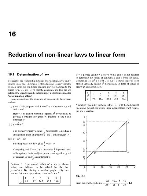
- Page 132 and 133: Reduction of non-linear laws to lin
- Page 134 and 135: Reduction of non-linear laws to lin
- Page 136 and 137: Reduction of non-linear laws to lin
- Page 138 and 139: Graphs with logarithmic scales 125
- Page 140 and 141: Graphs with logarithmic scales 127
- Page 142 and 143: Graphs with logarithmic scales 129
- Page 144 and 145: 18 Geometry and triangles 18.1 Angu
- Page 146 and 147: Geometry and triangles 133 (d) 227
- Page 148 and 149: Geometry and triangles 135 (a) Equi
- Page 150 and 151: Geometry and triangles 137 Hence XZ
- Page 152 and 153: Geometry and triangles 139 Now try
- Page 154 and 155: Geometry and triangles 141 Assignme
- Page 156 and 157: Introduction to trigonometry 143 Fr
- Page 158 and 159: Introduction to trigonometry 145 Si
- Page 160 and 161: Introduction to trigonometry 147 If
- Page 162 and 163: Introduction to trigonometry 149 To
- Page 164 and 165: 20 Trigonometric waveforms 20.1 Gra
- Page 166 and 167: Trigonometric waveforms 153 between
- Page 168 and 169: Trigonometric waveforms 155 45° 60
- Page 170 and 171: Trigonometric waveforms 157 y 4 0 y
- Page 172 and 173: Trigonometric waveforms 159 v rads/
- Page 174 and 175: Trigonometric waveforms 161 Assignm
- Page 176 and 177: Cartesian and polar co-ordinates 16
- Page 178 and 179: Cartesian and polar co-ordinates 16
- Page 180 and 181:
Areas of plane figures 167 W X Tabl
- Page 182 and 183:
Areas of plane figures 169 (b) Area
- Page 184 and 185:
Areas of plane figures 171 14. Calc
- Page 186 and 187:
Areas of plane figures 173 is 12 50
- Page 188 and 189:
The circle 175 Q B Now try the foll
- Page 190 and 191:
The circle 177 From equation (2), a
- Page 192 and 193:
The circle 179 Thus, for example, t
- Page 194 and 195:
Volumes of common solids 181 Proble
- Page 196 and 197:
Volumes of common solids 183 Proble
- Page 198 and 199:
Volumes of common solids 185 Fig. 2
- Page 200 and 201:
Volumes of common solids 187 From F
- Page 202 and 203:
Volumes of common solids 189 Volume
- Page 204 and 205:
25 Irregular areas and volumes and
- Page 206 and 207:
Irregular areas and volumes and mea
- Page 208 and 209:
Irregular areas and volumes and mea
- Page 210 and 211:
Irregular areas and volumes and mea
- Page 212 and 213:
Triangles and some practical applic
- Page 214 and 215:
Triangles and some practical applic
- Page 216 and 217:
Triangles and some practical applic
- Page 218 and 219:
Triangles and some practical applic
- Page 220 and 221:
27 Vectors 27.1 Introduction Some p
- Page 222 and 223:
Vectors 209 r 10° b Having obtaine
- Page 224 and 225:
Vectors 211 b Fig. 27.11 o Fig. 27.
- Page 226 and 227:
Vectors 213 N Thus the velocity of
- Page 228 and 229:
Adding of waveforms 215 y 6.1 6 4 2
- Page 230 and 231:
Adding of waveforms 217 The horizon
- Page 232 and 233:
Number sequences 219 The first four
- Page 234 and 235:
Number sequences 221 5. Determine t
- Page 236 and 237:
Number sequences 223 Hence 1 ( 1 9
- Page 238 and 239:
Number sequences 225 Now try the fo
- Page 240 and 241:
Presentation of statistical data 22
- Page 242 and 243:
Presentation of statistical data 22
- Page 244 and 245:
Presentation of statistical data 23
- Page 246 and 247:
Presentation of statistical data 23
- Page 248 and 249:
31 Measures of central tendency and
- Page 250 and 251:
Measures of central tendency and di
- Page 252 and 253:
Measures of central tendency and di
- Page 254 and 255:
32 Probability 32.1 Introduction to
- Page 256 and 257:
Probability 243 (a) The probability
- Page 258 and 259:
Probability 245 Two brass washers a
- Page 260 and 261:
33 Introduction to differentiation
- Page 262 and 263:
Introduction to differentiation 249
- Page 264 and 265:
Introduction to differentiation 251
- Page 266 and 267:
Introduction to differentiation 253
- Page 268 and 269:
Introduction to differentiation 255
- Page 270 and 271:
34 Introduction to integration 34.1
- Page 272 and 273:
Introduction to integration 259 ∫
- Page 274 and 275:
Introduction to integration 261 Pro
- Page 276 and 277:
Introduction to integration 263 A t
- Page 278 and 279:
Introduction to integration 265 Ass
- Page 280 and 281:
List of formulae 267 (ii) Parallelo
- Page 282 and 283:
List of formulae 269 Cartesian and
- Page 284 and 285:
Answers to exercises 271 Exercise 7
- Page 286 and 287:
Answers to exercises 273 7. ab 6 c
- Page 288 and 289:
Answers to exercises 275 5. 0.013 3
- Page 290 and 291:
Answers to exercises 277 Exercise 5
- Page 292 and 293:
Answers to exercises 279 Exercise 7
- Page 294 and 295:
Answers to exercises 281 Exercise 9
- Page 296 and 297:
Answers to exercises 283 Exercise 1
- Page 298 and 299:
Index Abscissa, 83 Acute angle, 132
- Page 300 and 301:
Index 287 Interior angles, 132, 134


![[Lonely Planet] Sri Lanka](https://img.yumpu.com/59845622/1/169x260/lonely-planet-sri-lanka.jpg?quality=85)