Climate change and water resources in the Murray Darling Basin ...
Climate change and water resources in the Murray Darling Basin ...
Climate change and water resources in the Murray Darling Basin ...

You also want an ePaper? Increase the reach of your titles
YUMPU automatically turns print PDFs into web optimized ePapers that Google loves.
ABARE CONFERENCE PAPER 02.11<br />
<strong>Climate</strong> <strong>change</strong> <strong>and</strong> <strong>water</strong> <strong>resources</strong> <strong>in</strong><br />
<strong>the</strong> <strong>Murray</strong> Darl<strong>in</strong>g Bas<strong>in</strong>, Australia<br />
Impacts <strong>and</strong> possible adaptation<br />
Stephen Beare <strong>and</strong> Anna Heaney<br />
Australian Bureau of Agricultural <strong>and</strong> Resource Economics<br />
2002 World Congress of Environmental <strong>and</strong> Resource Economists<br />
Monterey, California, 24–27 June 2002<br />
In Australia, <strong>change</strong>s to <strong>the</strong> hydrological cycle under conditions of enhanced<br />
global warm<strong>in</strong>g are likely to be complex <strong>and</strong> spatially diverse. While a number<br />
of emission scenarios have been developed to explore <strong>the</strong> key drivers of global<br />
warm<strong>in</strong>g, <strong>the</strong> capacity to adapt to climate <strong>change</strong> has not received <strong>the</strong> same<br />
level of attention.<br />
A simulation model was used to exam<strong>in</strong>e <strong>the</strong> potential impact of <strong>change</strong>s <strong>in</strong><br />
precipitation <strong>and</strong> evaporation for two scenarios developed by <strong>the</strong> Intergovernmental<br />
Panel on <strong>Climate</strong> Change. In <strong>the</strong> scenarios considered, precipitation<br />
is expected to decrease <strong>and</strong> evaporation to <strong>in</strong>crease over much of <strong>the</strong><br />
<strong>Murray</strong> Darl<strong>in</strong>g Bas<strong>in</strong> <strong>in</strong> <strong>the</strong> present century. The consequent reduction <strong>in</strong><br />
surface <strong>water</strong> flows over a relatively short time frame, coupled with <strong>the</strong> delayed<br />
effects of a reduction <strong>in</strong> ground <strong>water</strong> recharge, generates both positive <strong>and</strong><br />
negative economic <strong>and</strong> environmental impacts.<br />
Improved <strong>water</strong> use efficiency <strong>and</strong> <strong>the</strong> existence of an operational <strong>water</strong> market<br />
were explored as possible means of adapt<strong>in</strong>g to <strong>the</strong> decreas<strong>in</strong>g availability of<br />
surface <strong>water</strong> <strong>resources</strong> <strong>and</strong> were found to significantly mitigate <strong>the</strong> effects of<br />
a drier climate. However, both will require well def<strong>in</strong>ed <strong>and</strong> secure property<br />
rights to achieve <strong>the</strong> maximum economic benefit.<br />
ABARE project 2740<br />
1
ABARE CONFERENCE PAPER 02.11<br />
Introduction<br />
<strong>Climate</strong> <strong>change</strong> is expected to have significant impacts on <strong>the</strong> hydrological cycle at both a<br />
global <strong>and</strong> regional scale. This will <strong>in</strong> turn, affect <strong>the</strong> availability of, <strong>and</strong> dem<strong>and</strong> for, <strong>water</strong><br />
<strong>resources</strong> <strong>and</strong> <strong>the</strong> way <strong>the</strong> <strong>resources</strong> are most effectively managed. The Intergovernmental<br />
Panel on <strong>Climate</strong> Change (IPCC) was formed <strong>in</strong> 1988 to assess <strong>the</strong> nature <strong>and</strong> extent of<br />
global warm<strong>in</strong>g as well as options for mitigat<strong>in</strong>g <strong>and</strong> adapt<strong>in</strong>g to climate <strong>change</strong>. To date,<br />
<strong>the</strong> assessments have focused on establish<strong>in</strong>g <strong>the</strong> historical relationship between greenhouse<br />
gas emissions <strong>and</strong> global warm<strong>in</strong>g <strong>and</strong> project<strong>in</strong>g <strong>the</strong> impact of past <strong>and</strong> future emissions<br />
on <strong>the</strong> earth’s climate, <strong>and</strong> consequently on <strong>the</strong> mar<strong>in</strong>e <strong>and</strong> terrestrial environment.<br />
A number of future emission scenarios have been developed to explore <strong>the</strong> l<strong>in</strong>ks between<br />
global warm<strong>in</strong>g <strong>and</strong> economic development, population growth <strong>and</strong> technological progress.<br />
While none of <strong>the</strong>se scenarios is l<strong>in</strong>ked to specific policies to reduce emissions, <strong>the</strong>y have<br />
provided a range of possible outcomes aga<strong>in</strong>st which <strong>the</strong> benefits at a global <strong>and</strong> regional<br />
level of mitigat<strong>in</strong>g climate <strong>change</strong> can be assessed. However, <strong>the</strong> capacity to adapt to<br />
climate <strong>change</strong> has not received <strong>the</strong> same level of attention.<br />
This may, <strong>in</strong> part, reflect <strong>the</strong> fact that assess<strong>in</strong>g <strong>the</strong> potential <strong>and</strong> <strong>in</strong>centives to adjust to<br />
<strong>change</strong>s <strong>in</strong> climatic conditions requires <strong>the</strong> explicit consideration of <strong>the</strong> l<strong>in</strong>ks between<br />
biophysical <strong>change</strong>s <strong>in</strong> <strong>the</strong> environment, productivity <strong>and</strong> economic returns. In <strong>the</strong> contribution<br />
of Work<strong>in</strong>g Group II to <strong>the</strong> Third Assessment Report of <strong>the</strong> IPCC, Arnell <strong>and</strong><br />
Chunzhen (2001) reiterate this po<strong>in</strong>t, conclud<strong>in</strong>g that <strong>the</strong>re have been relatively few<br />
published studies on <strong>the</strong> impact of climate <strong>change</strong> on real world <strong>water</strong> resource systems<br />
<strong>and</strong> that most of <strong>the</strong>se studies ignore <strong>the</strong> potential for adaptation.<br />
The objective <strong>in</strong> this paper is to exam<strong>in</strong>e <strong>the</strong> impacts of climate <strong>change</strong> on <strong>the</strong> hydrological<br />
cycle, particularly stream <strong>and</strong> ground <strong>water</strong> flows, <strong>water</strong> quality <strong>and</strong> irrigated agriculture<br />
<strong>in</strong> Australia’s <strong>Murray</strong> Darl<strong>in</strong>g Bas<strong>in</strong>. The <strong>in</strong>tent is not to project <strong>the</strong> likely extent or<br />
range of possible climate outcomes but, first, to compare how different trends <strong>in</strong> global<br />
warm<strong>in</strong>g may affect economic <strong>and</strong> environmental outcomes <strong>in</strong> <strong>the</strong> bas<strong>in</strong> <strong>and</strong>, second, to<br />
exam<strong>in</strong>e <strong>the</strong> extent to which market based options, such as <strong>in</strong>vestments to <strong>in</strong>crease <strong>water</strong><br />
use efficiency <strong>and</strong> <strong>water</strong> trad<strong>in</strong>g, can be used to offset or enhance <strong>the</strong> economic impacts<br />
of climate <strong>change</strong>. These market based adaptations may, <strong>in</strong> turn, have positive or negative<br />
external effects on <strong>water</strong> flows <strong>and</strong> <strong>water</strong> quality that may warrant fur<strong>the</strong>r consideration.<br />
The approach taken was to, first, select a pair of contrast<strong>in</strong>g global warm<strong>in</strong>g scenarios<br />
from <strong>the</strong> Special Report on Emissions Scenarios (SRES) that reflected a plausible range of<br />
greenhouse gas emissions by <strong>the</strong> year 2100 (IPCC 2000). The Atmospheric Research<br />
Division of Australia’s Commonwealth Scientific <strong>and</strong> Industrial Research Organisation<br />
(CSIRO) has run global <strong>and</strong> regional climate models to develop long term projections for<br />
a variety of climatic variables such as precipitation, temperature <strong>and</strong> potential evaporation.<br />
Changes <strong>in</strong> <strong>the</strong>se variables have been derived us<strong>in</strong>g climate model simulations to<br />
2
ABARE CONFERENCE PAPER 02.11<br />
provide <strong>in</strong>formation on <strong>the</strong> magnitude of regional responses <strong>in</strong> terms of local <strong>change</strong> per<br />
degree of global warm<strong>in</strong>g on a 120 square kilometre grid for <strong>the</strong> <strong>Murray</strong> Darl<strong>in</strong>g Bas<strong>in</strong>.<br />
These climatic <strong>change</strong>s were <strong>in</strong>corporated <strong>in</strong>to <strong>the</strong> Sal<strong>in</strong>ity <strong>and</strong> L<strong>and</strong>use Simulation<br />
Analysis (SALSA) model, developed at <strong>the</strong> Australian Bureau of Agricultural <strong>and</strong> Resource<br />
Economics (ABARE) (Bell <strong>and</strong> Heaney 2001). This model comb<strong>in</strong>es simulation <strong>and</strong> optimisation<br />
techniques to represent <strong>the</strong> relationships between agricultural production systems<br />
<strong>and</strong> <strong>the</strong> hydrological cycle of river catchments.<br />
Key biophysical <strong>and</strong> economic results are presented for each scenario. The biophysical<br />
variables considered <strong>in</strong>clude river flows, salt loads <strong>and</strong> salt concentration at several locations<br />
on <strong>the</strong> <strong>Murray</strong> River. The economic variables under consideration <strong>in</strong>clude <strong>change</strong>s<br />
<strong>in</strong> net agricultural returns <strong>and</strong> <strong>the</strong> opportunity cost of irrigation <strong>water</strong>.<br />
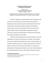
The <strong>Murray</strong> Darl<strong>in</strong>g Bas<strong>in</strong><br />
The <strong>Murray</strong> Darl<strong>in</strong>g Bas<strong>in</strong> covers more than one million square kilometres <strong>in</strong> south east<br />
Australia <strong>and</strong> accounts for around 14 per cent of Australia’s total l<strong>and</strong>mass (map 1). The<br />
bas<strong>in</strong> catchment conta<strong>in</strong>s Australia’s three largest rivers — <strong>the</strong> Darl<strong>in</strong>g, <strong>Murray</strong> <strong>and</strong><br />
Map 1: Major rivers <strong>in</strong> <strong>the</strong> <strong>Murray</strong> Darl<strong>in</strong>g Bas<strong>in</strong><br />
3
ABARE CONFERENCE PAPER 02.11<br />
Murrumbidgee — that collectively stretch for almost 7000 kilometres. Much of <strong>the</strong> bas<strong>in</strong><br />
is extensive pla<strong>in</strong>s <strong>and</strong> low undulat<strong>in</strong>g areas, mostly below 200 metres above sea level.<br />
An important consequence of <strong>the</strong> extent of <strong>the</strong> <strong>Murray</strong> Darl<strong>in</strong>g Bas<strong>in</strong> is <strong>the</strong> great range of<br />
climatic conditions <strong>and</strong> natural environments <strong>in</strong>clud<strong>in</strong>g ra<strong>in</strong>forests <strong>in</strong> <strong>the</strong> cool <strong>and</strong> humid<br />
eastern upl<strong>and</strong>s, <strong>the</strong> temperate mallee country of <strong>the</strong> south east, <strong>the</strong> subtropical areas of<br />
<strong>the</strong> north east as well as <strong>the</strong> semiarid <strong>and</strong> arid l<strong>and</strong>s of <strong>the</strong> far western pla<strong>in</strong>s.<br />
While <strong>the</strong> <strong>Murray</strong> Darl<strong>in</strong>g river system is large <strong>in</strong> terms of its catchment area <strong>and</strong> length,<br />
it is small <strong>in</strong> terms of surface <strong>water</strong> runoff. Almost 90 per cent of <strong>the</strong> bas<strong>in</strong> contributes<br />
virtually no runoff to <strong>the</strong> river systems, except at times of flood<strong>in</strong>g. The catchments dra<strong>in</strong><strong>in</strong>g<br />
<strong>the</strong> Great Divid<strong>in</strong>g Range — <strong>the</strong> Murrumbidgee, <strong>Murray</strong> <strong>and</strong> Goulburn–Broken —<br />
contribute almost half of <strong>the</strong> mean annual runoff while occupy<strong>in</strong>g only 11 per cent of <strong>the</strong><br />
area of <strong>the</strong> bas<strong>in</strong>. The variability of ra<strong>in</strong>fall <strong>in</strong> <strong>the</strong> bas<strong>in</strong> means that <strong>the</strong> river systems are<br />
subject to considerable variability of flows. Because of this large variation <strong>in</strong> stream flows,<br />
storage dams are needed to provide cont<strong>in</strong>uity of <strong>water</strong> supplies for urban, <strong>in</strong>dustrial <strong>and</strong><br />
agricultural uses. At <strong>the</strong> same time, <strong>the</strong> <strong>Murray</strong> Darl<strong>in</strong>g Bas<strong>in</strong> provides unique aquatic,<br />
terrestrial <strong>and</strong> wetl<strong>and</strong> habitats for native plants <strong>and</strong> animals.<br />
The <strong>Murray</strong> Darl<strong>in</strong>g Bas<strong>in</strong> accounts for more than 40 per cent of agricultural production <strong>in</strong><br />
Australia. Valued at an estimated A$34 billion, broadacre properties grazed around 5.9<br />
million beef cattle <strong>and</strong> 51 million sheep <strong>in</strong> 1999-2000. Wheat production exceeded 12<br />
million tonnes <strong>in</strong> <strong>the</strong> same year. While <strong>the</strong> <strong>Murray</strong> Darl<strong>in</strong>g Bas<strong>in</strong> is dom<strong>in</strong>ated by extensive<br />
dryl<strong>and</strong> agriculture, irrigated agriculture <strong>in</strong> <strong>the</strong> bas<strong>in</strong> accounts for around 70 per cent of<br />
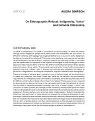
all <strong>water</strong> used <strong>in</strong> Australia (Crabb 1997). An estimated 1.3 million hectares was irrigated<br />
<strong>in</strong> 1996-97 with irrigated pasture account<strong>in</strong>g for more than 50 per cent of <strong>the</strong> total area<br />
irrigated (figure 1). River systems with<strong>in</strong> <strong>the</strong> <strong>Murray</strong> Darl<strong>in</strong>g Bas<strong>in</strong> provide domestic <strong>water</strong><br />
supplies to more than 10 per cent of <strong>the</strong> Australian population <strong>and</strong> support a range of<br />
<strong>in</strong>dustries.<br />
Figure 1: Area irrigated <strong>in</strong> <strong>the</strong> <strong>Murray</strong> Darl<strong>in</strong>g Bas<strong>in</strong>, by crop type<br />
700<br />
600<br />
500<br />
400<br />
300<br />
200<br />
100<br />
’000 ha<br />
Irrigated cotton<br />
Source: ABS Agricultural Census 1996-97<br />
Irrigated pasture<br />
4<br />
O<strong>the</strong>r irrigated crops
ABARE CONFERENCE PAPER 02.11<br />
Dem<strong>and</strong> for <strong>water</strong> is high <strong>in</strong> <strong>the</strong> <strong>Murray</strong> Darl<strong>in</strong>g Bas<strong>in</strong> <strong>and</strong> an audit of <strong>water</strong> use <strong>in</strong> 1995<br />
showed that if <strong>the</strong> volume of <strong>water</strong> diversions cont<strong>in</strong>ued to <strong>in</strong>crease, river health problems<br />
would be exacerbated, <strong>the</strong> security of <strong>water</strong> supply for exist<strong>in</strong>g users would be dim<strong>in</strong>ished,<br />
<strong>and</strong> <strong>the</strong> reliability of <strong>water</strong> supply dur<strong>in</strong>g long droughts would be reduced. Consequently,<br />
a cap was imposed on <strong>the</strong> volume of <strong>water</strong> that could be diverted from <strong>the</strong> rivers for<br />
consumptive uses. The cap limits fur<strong>the</strong>r <strong>in</strong>creases <strong>in</strong> <strong>water</strong> diversion but does not constra<strong>in</strong><br />
new developments provided <strong>the</strong>ir <strong>water</strong> requirements are met by us<strong>in</strong>g current allocations<br />
more efficiently or by purchas<strong>in</strong>g <strong>water</strong> from exist<strong>in</strong>g developments.<br />
Global climate <strong>change</strong> – <strong>the</strong> SRES scenarios<br />
The IPCC developed a series of greenhouse gas emission scenarios to reflect <strong>the</strong> current<br />
underst<strong>and</strong><strong>in</strong>g of <strong>the</strong> likely trends <strong>in</strong> future emissions <strong>and</strong> <strong>the</strong> uncerta<strong>in</strong>ties that surround<br />
<strong>the</strong>se trends. The differences <strong>in</strong> <strong>the</strong> scenarios are <strong>in</strong>tended to represent <strong>the</strong> range of uncerta<strong>in</strong>ty<br />
associated with <strong>the</strong> paths that <strong>the</strong> key drivers of emissions — population growth,<br />
economic growth <strong>and</strong> technological <strong>change</strong> — may take over <strong>the</strong> next century. There are<br />
four basic SRES storyl<strong>in</strong>es. At one extreme, high levels of both economic <strong>and</strong> population<br />
growth coupled with slow <strong>and</strong> limited adoption of clean, resource efficient technologies<br />
lead to <strong>the</strong> largest <strong>in</strong>crease <strong>in</strong> emissions. At <strong>the</strong> o<strong>the</strong>r extreme is a scenario with low population<br />
growth <strong>and</strong> a fairly rapid shift <strong>in</strong>to resource efficient technologies <strong>and</strong> a reduction <strong>in</strong><br />
<strong>the</strong> material <strong>in</strong>tensity with <strong>the</strong> use of pollution enhanc<strong>in</strong>g processes <strong>and</strong> materials.<br />
At <strong>the</strong> same time <strong>the</strong>re is considerable uncerta<strong>in</strong>ty about <strong>the</strong> extent of global warm<strong>in</strong>g<br />
associated with a given trend <strong>in</strong> emissions, <strong>and</strong> <strong>the</strong> sensitivity of <strong>the</strong> climate to greenhouse<br />
trends. For each of <strong>the</strong> four SRES storyl<strong>in</strong>es, a set of global climate <strong>change</strong> models was<br />
used to generate potential levels of global warm<strong>in</strong>g to <strong>the</strong> year 2100 for each scenario.<br />
The different models were used to establish high, medium <strong>and</strong> low levels of climate sensitivity<br />
for each scenario. The advantage of us<strong>in</strong>g several models was that <strong>the</strong> scenarios<br />
toge<strong>the</strong>r encompass <strong>the</strong> current range of uncerta<strong>in</strong>ties about future greenhouse gas emissions,<br />
<strong>in</strong> addition to <strong>the</strong> current knowledge of, <strong>and</strong> uncerta<strong>in</strong>ties associated with, <strong>the</strong> driv<strong>in</strong>g<br />
forces underly<strong>in</strong>g <strong>the</strong> scenarios.<br />
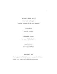
Over <strong>the</strong> full set of SRES scenarios <strong>and</strong> model projections, <strong>the</strong> level of global warm<strong>in</strong>g <strong>in</strong><br />
2100 ranges from 1.4 to 5.8°C relative to 1990. Figure 2 shows <strong>the</strong> envelope for projections<br />
<strong>in</strong> temperature rise under <strong>the</strong> SRES scenarios, with scenario A1F high generat<strong>in</strong>g<br />
<strong>the</strong> largest <strong>in</strong>creases <strong>in</strong> temperature, <strong>and</strong> B1 low <strong>the</strong> smallest <strong>in</strong>creases. The projections<br />
<strong>in</strong>dicate that warm<strong>in</strong>g will vary by region <strong>and</strong>, while overall precipitation is expected to<br />
<strong>in</strong>crease over <strong>the</strong> com<strong>in</strong>g century, <strong>the</strong>re are projected regional <strong>in</strong>creases <strong>and</strong> decreases <strong>in</strong><br />
average ra<strong>in</strong>fall over l<strong>and</strong> masses. Larger year to year variations <strong>in</strong> precipitation are very<br />
likely. The <strong>in</strong>tensity <strong>and</strong> frequency of extreme wea<strong>the</strong>r events is also expected to <strong>in</strong>crease<br />
(IPCC 2001).<br />
5
ABARE CONFERENCE PAPER 02.11<br />
The focus <strong>in</strong> this study is to exam<strong>in</strong>e how different global warm<strong>in</strong>g trends may affect <strong>the</strong><br />
hydrological cycle <strong>and</strong> agricultural production <strong>in</strong> <strong>the</strong> <strong>Murray</strong> Darl<strong>in</strong>g Bas<strong>in</strong>. It is not specifically<br />
concerned with <strong>the</strong> assumptions of economic, technological, demographic or o<strong>the</strong>r<br />
forces that underlie a specific emissions scenario. At <strong>the</strong> same time, it is useful to contrast<br />
a scenario that reflects an extension of <strong>the</strong> current trend <strong>in</strong> emissions to one <strong>in</strong> which <strong>the</strong>re<br />
has been a significant reduction <strong>in</strong> emissions.<br />
Two global warm<strong>in</strong>g curves were selected from with<strong>in</strong> <strong>the</strong> SRES envelope shown <strong>in</strong><br />
figure 2. The A1 scenario corresponds to a story l<strong>in</strong>e of high economic growth but with<br />
limited population growth, <strong>and</strong> <strong>the</strong> rapid <strong>in</strong>troduction of new <strong>and</strong> more efficient energy<br />
technologies. The B1 scenario corresponds to low population growth coupled with <strong>the</strong><br />
adoption of clean <strong>and</strong> resource efficient energy technologies. Estimates of temperature<br />
rise under both scenarios selected for this study are relatively conservative <strong>in</strong> comparison<br />
Figure 2: SRES global warm<strong>in</strong>g curves<br />
5<br />
4<br />
3<br />
2<br />
1<br />
ºC<br />
1990 2000 2010 2020 2030 2040 2050 2060 2070 2080 2090 2100<br />
with some of <strong>the</strong> more fossil fuel <strong>in</strong>tensive scenarios, with temperature predicted to <strong>in</strong>crease<br />
by 2.95°C by 2100 under scenario A1, <strong>and</strong> 1.98°C under scenario B1. The global warm<strong>in</strong>g<br />
curves selected for each scenario reflect a moderate level of sensitivity to <strong>change</strong>s <strong>in</strong> <strong>the</strong><br />
level of greenhouse gas emissions. The shape of <strong>the</strong> global warm<strong>in</strong>g curves suggests that<br />
much of <strong>the</strong> temperature <strong>in</strong>crease under scenario A1 happens <strong>in</strong> <strong>the</strong> latter half of <strong>the</strong> century<br />
whereas under scenario B1, temperature <strong>in</strong>creases steadily over <strong>the</strong> com<strong>in</strong>g 100 years.<br />
The shape of <strong>the</strong> curves, <strong>and</strong> hence <strong>the</strong> tim<strong>in</strong>g of <strong>the</strong> climate impacts, has important implications<br />
for both <strong>the</strong> biophysical <strong>and</strong> economic consequences of climate <strong>change</strong> <strong>in</strong> <strong>the</strong><br />
<strong>Murray</strong> Darl<strong>in</strong>g Bas<strong>in</strong>.<br />
6<br />
A1F high<br />
A1 mid<br />
B1 mid<br />
B1 low
ABARE CONFERENCE PAPER 02.11<br />
<strong>Climate</strong> <strong>change</strong> <strong>in</strong> <strong>the</strong> <strong>Murray</strong> Darl<strong>in</strong>g Bas<strong>in</strong><br />
Regional projections of climate <strong>change</strong> <strong>in</strong> Australia under <strong>the</strong> scenarios have been<br />
conducted by CSIRO. These studies use regional climate models, on ei<strong>the</strong>r a 125 kilometre<br />
or 60 square kilometre grid that have been nested with<strong>in</strong> <strong>the</strong> CSIRO Mark II global<br />
climate model. Changes <strong>in</strong> average annual precipitation <strong>and</strong> potential evaporation are<br />
calculated us<strong>in</strong>g OZCLIM, a climate <strong>change</strong> scenario generator developed at CSIRO (Walsh<br />
et al. 2001). The impacts of global warm<strong>in</strong>g on average annual precipitation <strong>in</strong> <strong>the</strong> <strong>Murray</strong><br />
Darl<strong>in</strong>g Bas<strong>in</strong> for years 2050 <strong>and</strong> 2100 are shown for each scenario <strong>in</strong> maps 2 to 5. For<br />
<strong>the</strong> <strong>Murray</strong> Darl<strong>in</strong>g Bas<strong>in</strong>, <strong>the</strong> midrange of <strong>the</strong>se projections <strong>in</strong>dicates that <strong>the</strong>re will be a<br />
general decl<strong>in</strong>e <strong>in</strong> precipitation <strong>and</strong> an <strong>in</strong>crease <strong>in</strong> potential evaporation. However, <strong>the</strong><br />
extent <strong>and</strong> tim<strong>in</strong>g of <strong>the</strong> decl<strong>in</strong>e <strong>in</strong> <strong>the</strong>se parameters varies across <strong>the</strong> bas<strong>in</strong> <strong>in</strong> l<strong>in</strong>e with<br />
<strong>the</strong> differences between <strong>the</strong> global warm<strong>in</strong>g curves.<br />
In scenario SRES A1, <strong>the</strong> decl<strong>in</strong>e <strong>in</strong> precipitation is projected to be less than 5 per cent <strong>in</strong><br />
2050 for almost all catchments except <strong>in</strong> those feed<strong>in</strong>g <strong>the</strong> Victorian tributaries of <strong>the</strong><br />
<strong>Murray</strong> River where <strong>the</strong> decl<strong>in</strong>e is expected to be between 5 <strong>and</strong> 10 per cent. Projected<br />
decl<strong>in</strong>es <strong>in</strong> precipitation under <strong>the</strong> SRES B1 scenario are less severe. By 2100, precipitation<br />
decl<strong>in</strong>es by between 5 <strong>and</strong> 10 per cent for most of <strong>the</strong> bas<strong>in</strong> <strong>and</strong> by up to 20 per cent<br />
<strong>in</strong> <strong>the</strong> Victorian tributaries of <strong>the</strong> <strong>Murray</strong> River under <strong>the</strong> A1 scenario. In contrast, many of<br />
<strong>the</strong> <strong>Murray</strong> River tributaries are projected to experience a decl<strong>in</strong>e <strong>in</strong> precipitation of less<br />
than 10 per cent by 2100 under <strong>the</strong> SRES B1 scenario, <strong>and</strong> by less than 5 per cent <strong>in</strong> almost<br />
all of <strong>the</strong> Darl<strong>in</strong>g River tributaries.<br />
Ra<strong>in</strong>fall distribution is also likely to vary under climate <strong>change</strong>. Summer ra<strong>in</strong>fall is expected<br />
to decl<strong>in</strong>e under both scenarios, particularly <strong>in</strong> <strong>the</strong> sou<strong>the</strong>rn reaches of <strong>the</strong> bas<strong>in</strong>. Reductions<br />
<strong>in</strong> summer ra<strong>in</strong>fall for <strong>the</strong> Darl<strong>in</strong>g River tributaries are expected to be between 1 <strong>and</strong> 7<br />
per cent under <strong>the</strong> A1 scenario <strong>and</strong> between 2 <strong>and</strong> 6 per cent for <strong>the</strong> B1 scenario <strong>in</strong> 2100.<br />
Victorian tributaries of <strong>the</strong> <strong>Murray</strong> River are expected to experience a decl<strong>in</strong>e <strong>in</strong> summer<br />
ra<strong>in</strong>fall under both scenarios by 2100. While climate <strong>change</strong> projections based on <strong>the</strong><br />
SRES scenarios do not yield conclusive results on <strong>the</strong> frequency of La Niña <strong>and</strong> El Niño<br />
events, <strong>the</strong> severity of both flood <strong>and</strong> droughts is expected to <strong>in</strong>crease.<br />
In addition to precipitation, climate <strong>change</strong> has an impact on temperature, humidity <strong>and</strong><br />
w<strong>in</strong>d speed, all of which have an impact potential evaporation. An <strong>in</strong>crease <strong>in</strong> annual average<br />
potential evaporation is expected over <strong>the</strong> whole bas<strong>in</strong> under both global warm<strong>in</strong>g<br />
scenarios by 2100, particularly <strong>in</strong> <strong>the</strong> <strong>Murray</strong> River tributary catchments. The impacts are<br />
greater under <strong>the</strong> A1 scenario, with <strong>in</strong>creases <strong>in</strong> potential evaporation of almost 20 per<br />
cent <strong>in</strong> many of <strong>the</strong> sou<strong>the</strong>rn reaches. On balance, <strong>the</strong> projections for <strong>the</strong> <strong>Murray</strong> Darl<strong>in</strong>g<br />
Bas<strong>in</strong> are for slight to moderate reductions <strong>in</strong> <strong>water</strong> availability for dryl<strong>and</strong> agriculture<br />
<strong>and</strong> moderate to substantial reductions <strong>in</strong> surface <strong>water</strong> flows. Increases <strong>in</strong> open <strong>water</strong><br />
evaporation will also affect effluent stream systems, <strong>water</strong> storages <strong>and</strong> wetl<strong>and</strong>s.<br />
7
ABARE CONFERENCE PAPER 02.11<br />
Map 2: Projected decl<strong>in</strong>e <strong>in</strong> precipitation <strong>in</strong> <strong>the</strong> <strong>Murray</strong> Darl<strong>in</strong>g Bas<strong>in</strong><br />
under SRES scenario A1, 2050<br />
Per cent decl<strong>in</strong>e from base:<br />
more than 20 per cent<br />
between 15 <strong>and</strong> 20 per cent<br />
between 10 <strong>and</strong> 15 per cent<br />
between 5 <strong>and</strong> 10 per cent<br />
less than 5 per cent<br />
Map 3: Projected decl<strong>in</strong>e <strong>in</strong> precipitation <strong>in</strong> <strong>the</strong> <strong>Murray</strong> Darl<strong>in</strong>g Bas<strong>in</strong><br />
under SRES scenario A1, 2100<br />
Per cent decl<strong>in</strong>e from base:<br />
more than 20 per cent<br />
between 15 <strong>and</strong> 20 per cent<br />
between 10 <strong>and</strong> 15 per cent<br />
between 5 <strong>and</strong> 10 per cent<br />
less than 5 per cent<br />
8<br />
MURRUMBIDGEE RIVER<br />
MURRUMBIDGEE RIVER
ABARE CONFERENCE PAPER 02.11<br />
Map 4: Projected decl<strong>in</strong>e <strong>in</strong> precipitation <strong>in</strong> <strong>the</strong> <strong>Murray</strong> Darl<strong>in</strong>g Bas<strong>in</strong><br />
under SRES scenario B1, 2050<br />
Per cent decl<strong>in</strong>e from base:<br />
more than 20 per cent<br />
between 15 <strong>and</strong> 20 per cent<br />
between 10 <strong>and</strong> 15 per cent<br />
between 5 <strong>and</strong> 10 per cent<br />
less than 5 per cent<br />
9<br />
MURRUMBIDGEE RIVER<br />
Map 5: Projected decl<strong>in</strong>e <strong>in</strong> precipitation <strong>in</strong> <strong>the</strong> <strong>Murray</strong> Darl<strong>in</strong>g Bas<strong>in</strong><br />
under SRES scenario B1, 2100<br />
Per cent decl<strong>in</strong>e from base:<br />
more than 20 per cent<br />
between 15 <strong>and</strong> 20 per cent<br />
between 10 <strong>and</strong> 15 per cent<br />
between 5 <strong>and</strong> 10 per cent<br />
less than 5 per cent<br />
MURRUMBIDGEE RIVER
ABARE CONFERENCE PAPER 02.11<br />
<strong>Climate</strong> <strong>change</strong> <strong>and</strong> <strong>water</strong> <strong>resources</strong><br />
Changes <strong>in</strong> precipitation are <strong>the</strong> prime driver of <strong>change</strong> <strong>in</strong> <strong>the</strong> availability of both surface<br />
<strong>and</strong> ground <strong>water</strong> <strong>resources</strong>. However, <strong>the</strong>re are a number of o<strong>the</strong>r factors that can significantly<br />
affect regional <strong>water</strong> balances that are likely to be <strong>in</strong>fluenced by climate <strong>change</strong>.<br />
With<strong>in</strong> a simple <strong>water</strong> balance model, <strong>the</strong> volume of <strong>water</strong> available as surface <strong>water</strong> <strong>and</strong><br />
ground <strong>water</strong> <strong>resources</strong> are <strong>the</strong> excess of precipitation over evapotranspiration. Climatic<br />
factors have a direct effect on evapotranspiration through <strong>change</strong>s <strong>in</strong> potential evaporation<br />
that occur with <strong>change</strong>s <strong>in</strong> solar radiation, humidity, temperature <strong>and</strong> w<strong>in</strong>d speed at<br />
ground level.<br />
Vegetation cover has a significant <strong>in</strong>fluence on evapotranspiration, with deep rooted trees<br />
<strong>and</strong> perennial species generally return<strong>in</strong>g more <strong>water</strong> to <strong>the</strong> atmosphere than annual grasses<br />
<strong>and</strong> o<strong>the</strong>r shallow rooted species. However, <strong>the</strong> <strong>in</strong>fluence of vegetation cover on transpiration<br />
<strong>in</strong>creases with higher precipitation (Zhang, Dawes <strong>and</strong> Walker 1999) <strong>and</strong> this may<br />
moderate <strong>the</strong> direct impacts of climate <strong>change</strong>. In low ra<strong>in</strong>fall areas (less than 500 millimetres<br />
a year), different vegetation covers transpire about <strong>the</strong> same volume of <strong>water</strong>. In areas<br />
with ra<strong>in</strong>fall above 500 millimetres a year, deep-rooted plants transpire an <strong>in</strong>creas<strong>in</strong>gly<br />
larger volume of <strong>water</strong> when compared with shallow rooted grasses. Changes <strong>in</strong> climatic<br />
conditions can, <strong>in</strong> turn, have an impact on ground cover <strong>and</strong> evapotranspiration. While <strong>the</strong><br />
physiological response of vegetation to <strong>in</strong>creased concentrations of atmospheric carbon<br />
dioxide is uncerta<strong>in</strong>, higher levels of carbon dioxide can result <strong>in</strong> greater levels of <strong>water</strong><br />
use efficiency by plants, result<strong>in</strong>g <strong>in</strong> reduced transpiration. At <strong>the</strong> same time, associated<br />
climatic effects such as higher temperatures, <strong>change</strong>s <strong>in</strong> ra<strong>in</strong>fall <strong>and</strong> soil moisture could<br />
ei<strong>the</strong>r enhance or negate potentially beneficial effects of higher carbon dioxide concentrations<br />
on plant physiology. Significant <strong>change</strong>s <strong>in</strong> temperature <strong>and</strong> precipitation may<br />
alter <strong>the</strong> species composition of ground cover <strong>and</strong>, hence, evapotranspiration also.<br />
Precipitation that is not returned to <strong>the</strong> atmosphere (excess) is ei<strong>the</strong>r transported as surface<br />
<strong>water</strong> runoff or enters <strong>the</strong> ground <strong>water</strong> system (ground <strong>water</strong> recharge). The fraction of<br />
this excess <strong>water</strong> that enters <strong>the</strong> ground <strong>water</strong> system depends on <strong>the</strong> rate of <strong>in</strong>filtration,<br />
<strong>the</strong> rate at which <strong>water</strong> can penetrate <strong>the</strong> soil surface <strong>and</strong> percolation through <strong>the</strong> soil<br />
profile. The rate of penetration depends on several factors <strong>in</strong>clud<strong>in</strong>g <strong>the</strong> slope or gradient<br />
of <strong>the</strong> l<strong>and</strong>, size, texture <strong>and</strong> structure of <strong>the</strong> soil particles <strong>and</strong> <strong>the</strong> level of soil moisture.<br />
On more steeply sloped l<strong>and</strong> <strong>the</strong>re tends to be fewer <strong>and</strong> smaller local depressions to store<br />
<strong>water</strong> that can <strong>the</strong>n <strong>in</strong>filtrate <strong>the</strong> soil. Clay soils have f<strong>in</strong>er soil particles creat<strong>in</strong>g smaller<br />
gaps through which <strong>water</strong> can enter <strong>and</strong> move through <strong>the</strong> soil profile. Under <strong>the</strong>se conditions<br />
most of <strong>the</strong> excess enters <strong>the</strong> river system as surface runoff. S<strong>and</strong>y <strong>and</strong> less compacted<br />
soils have larger gaps allow<strong>in</strong>g <strong>water</strong> to enter <strong>and</strong> move through <strong>the</strong> soil profile more easily<br />
than <strong>in</strong> heavier soils. Catchment runoff can be <strong>in</strong>significant on flat terra<strong>in</strong> with s<strong>and</strong>y soils.<br />
The <strong>in</strong>tensity, frequency <strong>and</strong> duration of ra<strong>in</strong>fall events affect soil moisture, <strong>and</strong> <strong>the</strong> likelihood<br />
of <strong>and</strong> extent to which <strong>the</strong> soil will become saturated.<br />
10
ABARE CONFERENCE PAPER 02.11<br />
Water dem<strong>and</strong><br />
Irrigated agriculture generates <strong>the</strong> largest consumptive dem<strong>and</strong> for surface <strong>and</strong> ground<br />
<strong>water</strong> <strong>resources</strong> <strong>in</strong> <strong>the</strong> <strong>Murray</strong> Darl<strong>in</strong>g Bas<strong>in</strong>. Around 10 000 gigalitres of surface <strong>water</strong><br />
is diverted for irrigation <strong>in</strong> <strong>the</strong> <strong>Murray</strong> Darl<strong>in</strong>g Bas<strong>in</strong> each year (MDBC 2002). While <strong>the</strong><br />
availability of <strong>water</strong> for irrigation is likely to decrease under conditions of reduced precipitation<br />
<strong>and</strong> <strong>in</strong>creased evapotranspiration, it is uncerta<strong>in</strong> how sensitive agricultural <strong>water</strong><br />
dem<strong>and</strong>s will be under enhanced greenhouse conditions. There are compet<strong>in</strong>g effects.<br />
First, decreased precipitation may lead to lower soil moisture profiles dur<strong>in</strong>g <strong>the</strong> irrigation<br />
season, depend<strong>in</strong>g on <strong>the</strong> tim<strong>in</strong>g of <strong>the</strong> ra<strong>in</strong>fall <strong>and</strong> <strong>the</strong> <strong>water</strong> hold<strong>in</strong>g capacity of <strong>the</strong><br />
soil. Second, <strong>in</strong>creases <strong>in</strong> potential evaporation through, for example, <strong>in</strong>creased temperature<br />
or reduced humidity, is likely to <strong>in</strong>crease losses from irrigation storages <strong>and</strong> channels.<br />
However, as noted previously, <strong>in</strong>creased atmospheric concentrations of carbon dioxide<br />
can lead to higher efficiency of plant <strong>water</strong> use, reduc<strong>in</strong>g <strong>the</strong> level of irrigation required<br />
to obta<strong>in</strong> a given yield.<br />
Case studies <strong>in</strong> <strong>the</strong> United States have produced some conflict<strong>in</strong>g results. In a climate<br />
<strong>change</strong> scenario <strong>in</strong>vestigated by Hatch et al. (1999), irrigation requirements were estimated<br />
to fall by as much as 30 per cent for corn <strong>in</strong> <strong>the</strong> south east United States. However,<br />
Ritschard et al. (1999) explored <strong>the</strong> same scenario <strong>and</strong> estimated that irrigation <strong>water</strong><br />
requirements would <strong>in</strong>crease. These studies <strong>in</strong>dicate <strong>the</strong> considerable uncerta<strong>in</strong>ty about<br />
future dem<strong>and</strong> for irrigation <strong>water</strong> <strong>and</strong>, hence, irrigation abstractions under conditions of<br />
enhanced global warm<strong>in</strong>g (Arnell <strong>and</strong> Chunzhen 2001).<br />
Water quality<br />
<strong>Climate</strong> <strong>change</strong> has <strong>the</strong> potential to make a significant impact on <strong>water</strong> quality <strong>in</strong> <strong>the</strong><br />
<strong>Murray</strong> Darl<strong>in</strong>g Bas<strong>in</strong>. As much of <strong>the</strong> cont<strong>in</strong>ent was covered by an <strong>in</strong>l<strong>and</strong> sea several<br />
millions of years ago, sal<strong>in</strong>e ground <strong>water</strong> systems are part of Australia’s geological legacy.<br />
Consequently, more than 25 per cent of Australia’s accessible ground <strong>water</strong> is above 1500<br />
milligrams of salt per litre (mg/L) <strong>and</strong> more than 10 per cent is <strong>in</strong> excess of 5000 mg/L<br />
(National L<strong>and</strong> <strong>and</strong> Water Resources Audit 2000). In irrigation areas along <strong>the</strong> south west<br />
reaches of <strong>the</strong> <strong>Murray</strong> River, ground <strong>water</strong> sal<strong>in</strong>ity levels are <strong>in</strong> excess of 30 000 mg/L,<br />
close to <strong>the</strong> salt concentration of sea<strong>water</strong>.<br />
Ris<strong>in</strong>g river sal<strong>in</strong>ity is a major <strong>water</strong> quality issue <strong>in</strong> <strong>the</strong> <strong>Murray</strong> Darl<strong>in</strong>g Bas<strong>in</strong>. L<strong>and</strong> clear<strong>in</strong>g<br />
<strong>and</strong> irrigation have <strong>in</strong>creased ground <strong>water</strong> recharge, which over time has led to ris<strong>in</strong>g<br />
<strong>water</strong> tables <strong>and</strong> <strong>in</strong>creased discharge of sal<strong>in</strong>e ground <strong>water</strong> <strong>in</strong>to rivers <strong>and</strong> streams.<br />
Consequently, <strong>the</strong> deterioration of river health ow<strong>in</strong>g to <strong>in</strong>creas<strong>in</strong>g sal<strong>in</strong>ity has been a<br />
concern to state <strong>and</strong> federal governments over recent years.<br />
11
ABARE CONFERENCE PAPER 02.11<br />
A sal<strong>in</strong>ity audit, released by <strong>the</strong> <strong>Murray</strong> Darl<strong>in</strong>g Bas<strong>in</strong> M<strong>in</strong>isterial Council <strong>in</strong> 1999,<br />
projected that salt mobilisation <strong>in</strong> <strong>the</strong> bas<strong>in</strong> would double from 5 million tonnes a year <strong>in</strong><br />
1998 to 10 million tonnes <strong>in</strong> 2100. Much of this <strong>in</strong>crease is likely to be mobilised from<br />
<strong>the</strong> irrigation areas that were developed with<strong>in</strong> 10 kilometres of <strong>the</strong> river <strong>in</strong> <strong>the</strong> south west<br />
reaches of <strong>the</strong> <strong>Murray</strong> River. This area, known as <strong>the</strong> Victorian Mallee <strong>and</strong> South Australian<br />
Riverl<strong>and</strong>, is characterised by extensive horticultural production. While <strong>the</strong>se regions often<br />
practise highly efficient irrigation us<strong>in</strong>g sophisticated irrigation schedul<strong>in</strong>g <strong>and</strong> delivery<br />
technology, <strong>the</strong>y overlay highly sal<strong>in</strong>e ground <strong>water</strong> aquifers <strong>and</strong> any ground <strong>water</strong> leakage<br />
results <strong>in</strong> large volumes of salt be<strong>in</strong>g mobilised to <strong>the</strong> <strong>Murray</strong> River. The audit also reported<br />
that <strong>the</strong> average sal<strong>in</strong>ity of <strong>the</strong> <strong>Murray</strong> River at Morgan, upstream of <strong>the</strong> major offtakes<br />
of <strong>water</strong> supplies to Adelaide, a city of more than one million people <strong>in</strong> South Australia,<br />
will exceed <strong>the</strong> 800 EC 1 World Health Organisation threshold for desirable dr<strong>in</strong>k<strong>in</strong>g <strong>water</strong><br />
quality <strong>in</strong> <strong>the</strong> next fifty to one hundred years (MDBMC 1999).<br />
Changes <strong>in</strong> climatic conditions will have both short <strong>and</strong> longer term impacts on river <strong>and</strong><br />
stream sal<strong>in</strong>ity. If, for example, <strong>the</strong>re is a reduction <strong>in</strong> precipitation, <strong>the</strong>re will be an immediate<br />
reduction <strong>in</strong> surface <strong>water</strong> runoff <strong>and</strong> less <strong>water</strong> available to dilute exist<strong>in</strong>g levels of<br />
sal<strong>in</strong>e ground <strong>water</strong> discharge. The decl<strong>in</strong>e <strong>in</strong> <strong>water</strong> quality will affect agriculture as <strong>the</strong><br />
productivity of <strong>water</strong> used for irrigation is reduced. It will also affect <strong>the</strong> river<strong>in</strong>e environment<br />
as well as urban <strong>and</strong> <strong>in</strong>dustrial <strong>water</strong> users.<br />
However, reductions <strong>in</strong> precipitation <strong>and</strong> <strong>in</strong>creases <strong>in</strong> evapotranspiration lead to reduced<br />
recharge that, over time, is reflected <strong>in</strong> a reduction <strong>in</strong> sal<strong>in</strong>e ground <strong>water</strong> discharge <strong>and</strong><br />
lower ground <strong>water</strong> tables. The length of <strong>the</strong> delay could range from a few years to several<br />
hundred years depend<strong>in</strong>g on <strong>the</strong> hydrological characteristics of <strong>the</strong> ground <strong>water</strong> flow<br />
system. The reduction <strong>in</strong> ground <strong>water</strong> discharge leads to benefits that are twofold. Sal<strong>in</strong>ity<br />
benefits are derived from <strong>the</strong> reduction <strong>in</strong> <strong>the</strong> discharge of sal<strong>in</strong>e <strong>water</strong> directly <strong>in</strong>to rivers<br />
<strong>and</strong> streams. Depend<strong>in</strong>g on <strong>the</strong> hydrological characteristics of <strong>the</strong> catchment, reductions <strong>in</strong><br />
salt mobilisation may translate <strong>in</strong>to lower salt concentrations even under conditions of<br />
reduced surface <strong>water</strong> flows. Sal<strong>in</strong>ity benefits are also derived if <strong>the</strong> reduction <strong>in</strong> discharge<br />
reduces <strong>the</strong> mobilisation of sal<strong>in</strong>e ground <strong>water</strong> <strong>in</strong>to <strong>the</strong> l<strong>and</strong>scape.<br />
Reductions <strong>in</strong> <strong>the</strong> area affected by dryl<strong>and</strong> sal<strong>in</strong>ity are likely to vary across <strong>the</strong> bas<strong>in</strong>, with<br />
<strong>the</strong> tim<strong>in</strong>g <strong>and</strong> extent dependent on <strong>the</strong> net effect of <strong>change</strong>s <strong>in</strong> <strong>the</strong> hydrological cycle, <strong>the</strong><br />
response time of <strong>the</strong> ground <strong>water</strong> flow system <strong>and</strong> <strong>the</strong> rate of recharge <strong>in</strong> each catchment.<br />
The impact of global warm<strong>in</strong>g on surface <strong>water</strong> <strong>and</strong> ground <strong>water</strong> flows, salt concentration<br />
<strong>and</strong> <strong>the</strong> area of high <strong>water</strong> tables under <strong>the</strong> SRES A1 <strong>and</strong> B1 scenarios are exam<strong>in</strong>ed<br />
us<strong>in</strong>g <strong>the</strong> SALSA model, described <strong>in</strong> <strong>the</strong> follow<strong>in</strong>g section.<br />
1 The most widely used method of estimat<strong>in</strong>g <strong>the</strong> sal<strong>in</strong>ity concentration of <strong>water</strong> is by electrical conductivity.<br />
To convert EC units to mg/L total dissolved salts, multiplication by a conversion factor of 0.6 generally<br />
applies.<br />
12
ABARE CONFERENCE PAPER 02.11<br />
The SALSA model<br />
The SALSA model<strong>in</strong>g framework was developed at ABARE, <strong>in</strong> cooperation with <strong>the</strong><br />
<strong>Murray</strong> Darl<strong>in</strong>g Bas<strong>in</strong> Commission <strong>and</strong> CSIRO L<strong>and</strong> <strong>and</strong> Water Division. The model was<br />
developed us<strong>in</strong>g <strong>the</strong> user <strong>in</strong>terface <strong>and</strong> simulation facilities of Extend (v4) (Imag<strong>in</strong>e That<br />
Inc. 1997). The model <strong>in</strong>corporates <strong>the</strong> relationships between l<strong>and</strong> use, vegetation cover,<br />
surface <strong>and</strong> ground <strong>water</strong> hydrology <strong>and</strong> agricultural returns. The bas<strong>in</strong> scale model consists<br />
of a network of l<strong>and</strong> management units l<strong>in</strong>ked through overl<strong>and</strong> <strong>and</strong> ground <strong>water</strong> flows.<br />
The geographic area under consideration is shown <strong>in</strong> map 6.<br />
The spatial coverage of <strong>the</strong> SALSA model <strong>in</strong>cludes <strong>the</strong> predom<strong>in</strong>antly dryl<strong>and</strong> regions of<br />
<strong>the</strong> <strong>Murray</strong> Darl<strong>in</strong>g Bas<strong>in</strong> spann<strong>in</strong>g from <strong>the</strong> Condam<strong>in</strong>e–Culgoa catchment <strong>in</strong> sou<strong>the</strong>rn<br />
Queensl<strong>and</strong> clockwise around <strong>the</strong> eastern edge of <strong>the</strong> bas<strong>in</strong> to <strong>the</strong> Avoca catchment <strong>in</strong><br />
Victoria. Irrigation with<strong>in</strong> each of <strong>the</strong>se catchments is also represented. The SALSA model<br />
also <strong>in</strong>cludes <strong>the</strong> Victorian Mallee <strong>and</strong> South Australian Riverl<strong>and</strong> irrigation areas immediately<br />
adjacent to <strong>the</strong> <strong>Murray</strong> River that extend from Nyah downstream to Morgan 2 . In<br />
Map 6: Cachments <strong>in</strong> <strong>the</strong> <strong>Murray</strong> Darl<strong>in</strong>g Bas<strong>in</strong> covered by <strong>the</strong> SALSA model<br />
2 All data presented for <strong>the</strong> Victorian Mallee <strong>and</strong> South Australian Riverl<strong>and</strong> refer to irrigation areas with<strong>in</strong><br />
10 kilometres of <strong>the</strong> <strong>Murray</strong> River. It is assumed that dryl<strong>and</strong> agriculture more than 10 kilometres from <strong>the</strong><br />
<strong>Murray</strong> River will not contribute salt loads to <strong>the</strong> river system.<br />
13
ABARE CONFERENCE PAPER 02.11<br />
<strong>the</strong> analysis presented here, 78 <strong>in</strong>dividual l<strong>and</strong> management units are def<strong>in</strong>ed accord<strong>in</strong>g<br />
to <strong>the</strong> characteristics of <strong>the</strong> ground <strong>water</strong> system — that is, <strong>the</strong>y are classified accord<strong>in</strong>g to<br />
whe<strong>the</strong>r <strong>the</strong>y are local, <strong>in</strong>termediate or regional flow systems.<br />
With<strong>in</strong> each l<strong>and</strong> management unit, economic models that optimise l<strong>and</strong> use are <strong>in</strong>tegrated<br />
with a representation of hydrological processes <strong>in</strong> each catchment. The hydrological component<br />
<strong>in</strong>corporates <strong>the</strong> relationships between irrigation, ra<strong>in</strong>fall, evapotranspiration <strong>and</strong><br />
surface <strong>water</strong> runoff, <strong>the</strong> effect of l<strong>and</strong> use <strong>change</strong> on ground <strong>water</strong> recharge <strong>and</strong> discharge<br />
rates, <strong>and</strong> <strong>the</strong> processes govern<strong>in</strong>g salt accumulation <strong>in</strong> streams <strong>and</strong> soil. The <strong>in</strong>teractions<br />
between precipitation, vegetation cover, surface <strong>water</strong> flows, ground <strong>water</strong> processes <strong>and</strong><br />
agricultural production are modeled at a river reach scale. In turn, <strong>the</strong>se reaches are l<strong>in</strong>ked<br />
through a network of surface <strong>and</strong> ground <strong>water</strong> flows.<br />
In <strong>the</strong> agroeconomic component of <strong>the</strong> model, l<strong>and</strong> is allocated to maximise economic<br />
return from <strong>the</strong> comb<strong>in</strong>ed use of agricultural l<strong>and</strong> <strong>and</strong> irrigation <strong>water</strong>. Each l<strong>and</strong> management<br />
unit is managed <strong>in</strong>dependently to maximise returns given <strong>the</strong> level of sal<strong>in</strong>ity of available<br />
l<strong>and</strong> <strong>and</strong> surface <strong>and</strong> ground <strong>water</strong> <strong>resources</strong>, subject to any l<strong>and</strong> use constra<strong>in</strong>ts.<br />
Incorporated <strong>in</strong> this component is <strong>the</strong> relationship between sal<strong>in</strong>ity <strong>and</strong> yield loss for each<br />
agricultural activity. Thus, l<strong>and</strong> use can shift with <strong>change</strong>s <strong>in</strong> <strong>the</strong> availability <strong>and</strong> quality of<br />
both l<strong>and</strong> <strong>and</strong> <strong>water</strong> <strong>resources</strong>. The cost of sal<strong>in</strong>ity is measured as <strong>the</strong> reduction <strong>in</strong> economic<br />
returns from agricultural activities from those that are currently earned. Some key features<br />
of <strong>the</strong> model are described briefly below. A full description is given <strong>in</strong> Bell <strong>and</strong> Heaney<br />
(2001).<br />
Hydrological component<br />
The hydrological component of <strong>the</strong> model consists of three parts. The first determ<strong>in</strong>es <strong>the</strong><br />
distribution of precipitation <strong>and</strong> irrigation <strong>water</strong> between evaporation <strong>and</strong> transpiration,<br />
surface <strong>water</strong> runoff <strong>and</strong> ground <strong>water</strong> recharge. With<strong>in</strong> this component of <strong>the</strong> model <strong>the</strong>re<br />
are two climatic drivers that are specified uniquely for each hydrologically def<strong>in</strong>ed l<strong>and</strong><br />
management unit — average annual ra<strong>in</strong>fall <strong>and</strong> evapotranspiration — specified as a function<br />
of ra<strong>in</strong>fall <strong>and</strong> l<strong>and</strong> cover.<br />
In <strong>the</strong> <strong>in</strong>itial specification of <strong>the</strong> SALSA model, <strong>the</strong> Holmes–S<strong>in</strong>clair relationship was<br />
used to specify <strong>the</strong> l<strong>in</strong>k between ground cover <strong>and</strong> evapotranspiration. For a given ground<br />
cover, <strong>the</strong> Holmes–S<strong>in</strong>clair relationship (estimated by Zhang et al. 1999) relates evapotranspiration<br />
to precipitation. The relationship does not <strong>in</strong>clude variation <strong>in</strong> potential evaporation,<br />
as it was not found to be a significant discrim<strong>in</strong>ator. However, <strong>in</strong> <strong>the</strong> climate <strong>change</strong><br />
scenarios that were evaluated, projected <strong>change</strong>s <strong>in</strong> potential evaporation were large <strong>in</strong><br />
comparison with projected <strong>change</strong>s <strong>in</strong> precipitation us<strong>in</strong>g <strong>the</strong> Holmes–S<strong>in</strong>clair relationship.<br />
14
ABARE CONFERENCE PAPER 02.11<br />
A study conducted by Hassel <strong>and</strong> Associates (1998) estimated <strong>the</strong> impact of high <strong>and</strong> low<br />
climate <strong>change</strong> scenarios on surface <strong>water</strong> runoff <strong>in</strong> <strong>the</strong> Macquarie–Bogan catchment of<br />
New South Wales. The study used a Sacramento model (Burnash, Ferral <strong>and</strong> McGuire<br />
1984) that <strong>in</strong>corporates <strong>change</strong>s <strong>in</strong> potential evaporation to estimate catchment runoff.<br />
Runoff was <strong>the</strong>n used to generate stream flows that were calibrated us<strong>in</strong>g <strong>the</strong> IQQM daily<br />
flow model (New South Wales Department of L<strong>and</strong> <strong>and</strong> Water Conservation 1995). The<br />
Sacramento model generated <strong>change</strong>s <strong>in</strong> stream flows that were approximately three times<br />
greater that would be predicted us<strong>in</strong>g <strong>the</strong> Holmes–S<strong>in</strong>clair relationship.<br />
Given <strong>the</strong> likely sensitivity of <strong>the</strong> analysis to <strong>the</strong> <strong>in</strong>corporation of potential evaporation,<br />
<strong>the</strong> Holmes–S<strong>in</strong>clair evapotranspiration relationship used <strong>in</strong> <strong>the</strong> SALSA model was modified<br />
to account for <strong>change</strong>s <strong>in</strong> potential evaporation. The relationships for tree <strong>and</strong> grass<br />
covered catchments provided <strong>the</strong> envelope for all o<strong>the</strong>r groundcovers used <strong>in</strong> <strong>the</strong> SALSA<br />
model. (The relationship between precipitation <strong>and</strong> evapotranspiration for all o<strong>the</strong>r groundcovers<br />
was specified as a l<strong>in</strong>ear comb<strong>in</strong>ation of <strong>the</strong> relationships for trees <strong>and</strong> grass.)<br />
The relationship for tree cover was specified as:<br />
(1)<br />
where<br />
<strong>and</strong> ppt is average annual precipitation, α is a parameter, PE is potential evaporation <strong>and</strong><br />
t denotes time <strong>in</strong> years. The relationship for grass cover was specified as:<br />
(2)<br />
⎛ ∆2800⎞ ⎛ ∆2800<br />
ppt ⎞<br />
ETTrees = ppt⎜1<br />
+ ⎟ ⎜1<br />
+ + ⎟<br />
⎝ ppt ⎠⎝<br />
ppt ∆400⎠<br />
∆= 1 + α PEt<br />
PE<br />
⎛ ∆2200⎞ ⎛ ∆2200<br />
ppt ⎞<br />
ETGrass = ppt⎜1<br />
+ ⎟ ⎜1<br />
+ + ⎟<br />
⎝ ppt ⎠⎝<br />
ppt ∆1100⎠<br />
An α of 0 gives <strong>the</strong> orig<strong>in</strong>al Holmes–S<strong>in</strong>clair specification <strong>and</strong> a value of 1.0 provided a<br />
reasonable fit to <strong>the</strong> runoff relationships generated by <strong>the</strong> IQQM model <strong>in</strong> <strong>the</strong> Macquarie–<br />
Bogan catchment. An α value of 1.0 was used for <strong>the</strong> simulations conducted <strong>and</strong> reported<br />
here. A simulation us<strong>in</strong>g <strong>the</strong> orig<strong>in</strong>al Holmes–S<strong>in</strong>clair specification is reported <strong>in</strong> appendix<br />
A for comparison.<br />
The second hydrological component of <strong>the</strong> model determ<strong>in</strong>es surface <strong>water</strong> runoff <strong>and</strong><br />
ground <strong>water</strong> recharge. The distribution of <strong>the</strong> excess between surface <strong>and</strong> ground <strong>water</strong><br />
recharge is assumed to be a constant proportion. For example, on heavier, less permeable<br />
soils on <strong>the</strong> steeper terra<strong>in</strong> of <strong>the</strong> upl<strong>and</strong> catchment areas, ground <strong>water</strong> recharge fractions<br />
range from 10 to 30 per cent. On <strong>the</strong> s<strong>and</strong>ier, more permeable soils on flat terra<strong>in</strong> <strong>in</strong> <strong>the</strong><br />
low ly<strong>in</strong>g catchment areas, recharge fractions were between 80 <strong>and</strong> 100 per cent.<br />
15<br />
t = 0<br />
−1<br />
−1
ABARE CONFERENCE PAPER 02.11<br />
The third part of <strong>the</strong> hydrology component determ<strong>in</strong>es ground <strong>water</strong> discharge <strong>in</strong>to streams<br />
<strong>and</strong> <strong>in</strong>to <strong>the</strong> l<strong>and</strong>scape <strong>in</strong> <strong>the</strong> form of high <strong>water</strong> tables. The equilibrium response time of<br />
a ground <strong>water</strong> flow system is <strong>the</strong> time it takes for a <strong>change</strong> <strong>in</strong> <strong>the</strong> rate of recharge to be<br />
fully reflected <strong>in</strong> a <strong>change</strong> <strong>in</strong> <strong>the</strong> rate of discharge. The equilibrium response time does<br />
not reflect <strong>the</strong> actual flow of <strong>water</strong> through <strong>the</strong> ground <strong>water</strong> system but <strong>the</strong> transmission<br />
of <strong>water</strong> pressure.<br />
Assum<strong>in</strong>g <strong>the</strong> contributions of recharge are additive <strong>and</strong> uncorrelated over time, it is possible<br />
to model gross discharge directly, <strong>the</strong>reby avoid<strong>in</strong>g <strong>the</strong> need to explicitly model ground<br />
<strong>water</strong> levels. In <strong>the</strong> approach adopted here, total discharge rate D <strong>in</strong> year t is a logistic<br />
function of a mov<strong>in</strong>g average of recharge rates <strong>in</strong> <strong>the</strong> current <strong>and</strong> earlier years accord<strong>in</strong>g to:<br />
(3)<br />
Dt () = R(<br />
0)+<br />
t<br />
∑<br />
i= t−m Ri () − Ri ( −1)<br />
1 + exp v −i<br />
/ v<br />
[ ( half ) slope]<br />
where R(0) is <strong>the</strong> <strong>in</strong>itial equilibrium recharge rate, m is <strong>the</strong> number of terms <strong>in</strong>cluded <strong>in</strong><br />
<strong>the</strong> mov<strong>in</strong>g average calculation, <strong>and</strong> ν half <strong>and</strong> ν slope are <strong>the</strong> time response parameters. The<br />
mov<strong>in</strong>g average formulation allows <strong>the</strong> accumulated impacts of past l<strong>and</strong> use <strong>change</strong> to<br />
be <strong>in</strong>corporated, as well as to model prospective <strong>change</strong>s.<br />
Ground <strong>water</strong> response times with<strong>in</strong> <strong>the</strong> <strong>Murray</strong> Darl<strong>in</strong>g Bas<strong>in</strong> vary substantially. In <strong>the</strong><br />
upl<strong>and</strong> areas, <strong>the</strong>re tends to be greater hydraulic head <strong>and</strong> shorter lateral flow distances to<br />
<strong>the</strong> po<strong>in</strong>t of discharge, predom<strong>in</strong>antly <strong>in</strong>to small streams. Average equilibrium response<br />
times <strong>in</strong> <strong>the</strong>se areas range between 60 <strong>and</strong> 120 years. In <strong>the</strong> low ly<strong>in</strong>g catchment areas,<br />
where <strong>the</strong>re is very little hydraulic head <strong>and</strong> lateral flow distances are long, equilibrium<br />
response times can be well <strong>in</strong> excess of 1000 years. In established irrigation areas <strong>the</strong> soil<br />
can be saturated <strong>and</strong> <strong>the</strong> ground <strong>water</strong> system nearly pressurised. Equilibrium response<br />
times under <strong>the</strong>se conditions are much faster, of <strong>the</strong> order of twenty to forty years.<br />
Agroeconomic component<br />
Changes <strong>in</strong> <strong>water</strong> availability, quality <strong>and</strong> <strong>the</strong> emergence of high <strong>water</strong> tables all have an<br />
impact on agricultural productivity. The agroeconomic component of <strong>the</strong> model seeks to<br />
maximise <strong>the</strong> returns to agriculture under <strong>the</strong> current conditions of <strong>the</strong> resource base. The<br />
management problem considered <strong>in</strong> <strong>the</strong> agroeconomic component of <strong>the</strong> model is that of<br />
maximis<strong>in</strong>g <strong>the</strong> economic return from <strong>the</strong> use of agricultural l<strong>and</strong> by choos<strong>in</strong>g between<br />
alternative steady state l<strong>and</strong> use activities <strong>in</strong> each year. Five l<strong>and</strong> use activities are considered<br />
— irrigated crops, irrigated pasture, irrigated horticulture, dryl<strong>and</strong> crops <strong>and</strong> dryl<strong>and</strong><br />
pasture.<br />
Each l<strong>and</strong> management unit is assumed to allocate its available l<strong>and</strong> each year between<br />
<strong>the</strong> above activities to maximise <strong>the</strong> net return from <strong>the</strong> use of <strong>the</strong> l<strong>and</strong> <strong>in</strong> production,<br />
16
ABARE CONFERENCE PAPER 02.11<br />
subject to constra<strong>in</strong>ts on <strong>the</strong> overall availability of irrigation <strong>water</strong> from rivers, sw*, <strong>and</strong><br />
from ground <strong>water</strong> sources, gw*, <strong>and</strong> suitable l<strong>and</strong>, L*:<br />
(4)<br />
subject to<br />
(5)<br />
where x j is output of activity j, L j is l<strong>and</strong> used <strong>in</strong> activity j, sw j is surface <strong>water</strong> <strong>and</strong> gw j is<br />
ground <strong>water</strong> used for irrigation of activity j, r is <strong>the</strong> discount rate, <strong>and</strong> csw is <strong>the</strong> unit cost<br />
of surface <strong>water</strong> used for irrigation <strong>and</strong> cgw is <strong>the</strong> unit cost of ground <strong>water</strong> used for irrigation.<br />
The net return to output for each activity is given by p j <strong>and</strong> is def<strong>in</strong>ed as <strong>the</strong> revenue<br />
from output less <strong>the</strong> cost of <strong>in</strong>puts, o<strong>the</strong>r than l<strong>and</strong> <strong>and</strong> <strong>water</strong>, per unit of output.<br />
For each activity, <strong>the</strong> volume of output depends on l<strong>and</strong> <strong>and</strong> <strong>water</strong> use (or on a subset of<br />
<strong>the</strong>se <strong>in</strong>puts) accord<strong>in</strong>g to a Cobb-Douglas production function:<br />
(6)<br />
where A j , α Lj , α swj <strong>and</strong> α gwj are technical coefficients <strong>in</strong> <strong>the</strong> production function. Note, <strong>the</strong><br />
technical coefficients on surface irrigation <strong>water</strong> are time dependent, to capture <strong>the</strong> impact<br />
of <strong>change</strong>s <strong>in</strong> salt concentration <strong>in</strong> <strong>the</strong> <strong>Murray</strong> River.<br />
The costs to irrigated agriculture <strong>and</strong> horticulture result<strong>in</strong>g from yield reductions caused by<br />
<strong>in</strong>creased river sal<strong>in</strong>ity are modeled explicitly. The impact of sal<strong>in</strong>e <strong>water</strong> on <strong>the</strong> productivity<br />
of plants is assumed to occur as plants extract sal<strong>in</strong>e <strong>water</strong> from <strong>the</strong> soil. The electroconductivity,<br />
EC, of <strong>the</strong> soil reflects <strong>the</strong> concentration of salt <strong>in</strong> <strong>the</strong> soil <strong>water</strong> <strong>and</strong> reduces<br />
<strong>the</strong> level of output per unit of l<strong>and</strong> <strong>in</strong>put (l<strong>and</strong> yield) <strong>and</strong> per unit of <strong>water</strong> <strong>in</strong>put (<strong>water</strong><br />
yield). This is represented by modify<strong>in</strong>g <strong>the</strong> appropriate technical coefficients, α swj , <strong>in</strong> <strong>the</strong><br />
production function for each activity from <strong>the</strong> level of those coefficients <strong>in</strong> <strong>the</strong> absence of<br />
sal<strong>in</strong>ity impacts. That is:<br />
(7)<br />
x<br />
j<br />
1<br />
max ∑ p x ( L , sw , gw )−csw∑ sw −cgw∑ gw<br />
r<br />
j<br />
j j j j j j j<br />
j<br />
j<br />
∑ j ∑ j ∑<br />
j<br />
j<br />
j<br />
sw ≤ sw*, gw ≤ gw * <strong>and</strong> L ≤ L *<br />
αLj αswj () t αgwj<br />
⎧<br />
⎪AjLj<br />
swj gwj 0< αLj + αswj + αgwj<br />
< 1for j = 12 , , 3<br />
= ⎨ α Lj<br />
⎩⎪ AL j j 0< α Lj < 1 for j=<br />
4, 5<br />
α<br />
swj<br />
max<br />
α swj<br />
() t =<br />
+ exp µ + µ<br />
1 ( 0j 1jEC)<br />
where µ 0j <strong>and</strong> µ 1j are productivity impact coefficients determ<strong>in</strong>ed for each activity <strong>and</strong><br />
α swj max is <strong>the</strong> level of <strong>the</strong> technical coefficient <strong>in</strong> <strong>the</strong> absence of sal<strong>in</strong>ity.<br />
17<br />
l
ABARE CONFERENCE PAPER 02.11<br />
Model calibration<br />
The data required to calibrate <strong>the</strong> model are extensive. The calibration procedure is given<br />
<strong>in</strong> Bell <strong>and</strong> Heaney (2001). The key physical data were historical ra<strong>in</strong>fall, stream flow <strong>and</strong><br />
salt load, <strong>and</strong> projected salt loads <strong>and</strong> areas of high <strong>water</strong> tables. Historical flows <strong>and</strong> salt<br />
loads were obta<strong>in</strong>ed from Jolly et al. (1997). Projected salt loads were obta<strong>in</strong>ed from <strong>the</strong><br />
national sal<strong>in</strong>ity audit (MDBMC 1999), Barnett et al. (2000) <strong>and</strong> Queensl<strong>and</strong> Department<br />
of Natural Resources (2001). These data, <strong>in</strong> comb<strong>in</strong>ation with <strong>the</strong> expertise of consult<strong>in</strong>g<br />
ground <strong>water</strong> hydrologists, were used to determ<strong>in</strong>e <strong>the</strong> hydrological parameters of <strong>the</strong><br />
model.<br />
Agroeconomic data were obta<strong>in</strong>ed from a wide range of sources. L<strong>and</strong> <strong>and</strong> <strong>water</strong> use data<br />
were obta<strong>in</strong>ed from many sources <strong>in</strong>clud<strong>in</strong>g ABARE farm survey data, Australian Bureau<br />
of Statistics Agricultural Census data <strong>and</strong> regional <strong>water</strong> authorities. Farm survey data<br />
were <strong>the</strong> primary source of <strong>the</strong> data used to estimate <strong>the</strong> fully capitalised returns to various<br />
l<strong>and</strong> use activities <strong>in</strong> <strong>the</strong> model. These returns were <strong>the</strong>n used to calibrate <strong>the</strong> production<br />
functions.<br />
To calculate <strong>in</strong>itial values for <strong>the</strong> production function parameters <strong>in</strong> (6), <strong>the</strong> total rent at<br />
full equity accru<strong>in</strong>g to each activity was first calculated as <strong>the</strong> summation of rent associated<br />
with <strong>the</strong> use of l<strong>and</strong> <strong>and</strong> o<strong>the</strong>r fixed <strong>in</strong>puts to production <strong>and</strong> surface <strong>and</strong> ground <strong>water</strong>.<br />
That is:<br />
(8)<br />
where<br />
(9)<br />
RentTotal = RentL + RentSW + RentGW + RentO<strong>the</strong>r<br />
j j j j j<br />
RentLj<br />
= Lj( 0)<br />
pm<strong>in</strong><br />
RentSWj<br />
= swj( 0)<br />
csw ˜<br />
RentGW<br />
= gw ( 0)<br />
cgw ˜<br />
j j<br />
RentO<strong>the</strong>r<br />
= L ( 0)<br />
p − p<br />
j j j<br />
( m<strong>in</strong>)<br />
where pm<strong>in</strong> is <strong>the</strong> net return to l<strong>and</strong> <strong>and</strong> o<strong>the</strong>r fixed capital structures <strong>in</strong> <strong>the</strong>ir marg<strong>in</strong>al use<br />
<strong>and</strong> csw ˜ is <strong>the</strong> opportunity cost of surface <strong>water</strong> used for irrigation <strong>and</strong> cgw ˜ is <strong>the</strong> opportunity<br />
cost of ground <strong>water</strong> used for irrigation <strong>in</strong> <strong>the</strong> <strong>in</strong>itial period. Data on <strong>the</strong> marg<strong>in</strong>al<br />
value of agricultural l<strong>and</strong> <strong>in</strong> Australia are not generally available; hence it was simply<br />
assumed that <strong>the</strong> marg<strong>in</strong>al value was 50 per cent of <strong>the</strong> average return from <strong>the</strong> lowest<br />
return<strong>in</strong>g activity. Trade prices for permanent <strong>water</strong> entitlements are a potential source of<br />
<strong>in</strong>formation on <strong>the</strong> opportunity costs of irrigation <strong>water</strong>. However, <strong>the</strong>re are significant<br />
physical <strong>and</strong> <strong>in</strong>stitutional constra<strong>in</strong>ts on <strong>water</strong> trade between catchments <strong>in</strong> <strong>the</strong> <strong>Murray</strong><br />
Darl<strong>in</strong>g Bas<strong>in</strong> <strong>and</strong> trade, to date, has been limited. In regions where <strong>the</strong>re are large volumes<br />
of <strong>water</strong> used to produce irrigated pasture <strong>and</strong> cereal crops, <strong>the</strong> annual opportunity cost<br />
of <strong>water</strong> was assumed to be <strong>in</strong> <strong>the</strong> range $20–30 a megalitre. In cotton <strong>and</strong> horticultural<br />
18
ABARE CONFERENCE PAPER 02.11<br />
areas <strong>the</strong> opportunity cost of <strong>water</strong> was assumed to be considerably higher at $70 <strong>and</strong> $150<br />
a megalitre respectively.<br />
Initial values for <strong>the</strong> production function coefficients for each activity were <strong>the</strong>n determ<strong>in</strong>ed<br />
as:<br />
RentLj<br />
α Lj(<br />
0)<br />
=<br />
RentTotalj<br />
RentSWj<br />
(10)<br />
α swj(<br />
0)<br />
=<br />
RentTotalj<br />
RentGWj<br />
α gwj(<br />
0)<br />
=<br />
RentTotal<br />
j<br />
1−αLj ( 0) −αswj ( 0) −αgwj<br />
( 0)<br />
j = j( 0) j( 0) j(<br />
0)<br />
A L sw gw<br />
With<strong>in</strong> a simulation, <strong>the</strong>se coefficients are adjusted from <strong>the</strong> <strong>in</strong>itial values accord<strong>in</strong>g to<br />
equation (6). The coefficients <strong>in</strong> equation (6) were derived from estimated yield losses<br />
caused by irrigation sal<strong>in</strong>ity (MDBC 1999).<br />
The <strong>Murray</strong> Darl<strong>in</strong>g Bas<strong>in</strong> Commission has l<strong>in</strong>ked its hydrological model<strong>in</strong>g to estimates<br />
of cost impacts based on <strong>in</strong>cremental <strong>in</strong>creases <strong>in</strong> sal<strong>in</strong>ity. Costs downstream of Morgan are<br />
imputed as a function of EC <strong>change</strong>s <strong>in</strong> salt concentration at Morgan. The analysis considers<br />
agricultural, domestic <strong>and</strong> <strong>in</strong>dustrial <strong>water</strong> uses. Us<strong>in</strong>g <strong>the</strong> cost functions derived <strong>in</strong><br />
this model, each unit <strong>in</strong>crease <strong>in</strong> EC at Morgan is imputed to have a downstream cost of<br />
$173 450 (Doug Young, Primary Resources South Australia, personal communication,<br />
January 2002). This cost is <strong>in</strong>cluded <strong>in</strong> <strong>the</strong> analysis presented here.<br />
Changes <strong>in</strong> annual average precipitation <strong>and</strong> potential evaporation were estimated for <strong>the</strong><br />
SRES climate <strong>change</strong> scenarios us<strong>in</strong>g <strong>the</strong> scenario generator OZCLIM version 2.0.1.<br />
Changes <strong>in</strong> <strong>the</strong>se variables were estimated as percentage <strong>change</strong>s from <strong>the</strong> base year 1995<br />
for <strong>the</strong> years 2020, 2050 <strong>and</strong> 2100. The <strong>in</strong>terven<strong>in</strong>g years were l<strong>in</strong>early <strong>in</strong>terpolated. The<br />
output generated by OZCLIM was <strong>the</strong>n translated <strong>in</strong>to a GIS po<strong>in</strong>t coverage us<strong>in</strong>g ArcInfo.<br />
Precipitation <strong>and</strong> potential evaporation data were extracted for each <strong>the</strong> l<strong>and</strong> management<br />
unit <strong>in</strong> <strong>the</strong> SALSA model us<strong>in</strong>g ArcView3.1. These data were <strong>in</strong>corporated <strong>in</strong>to <strong>the</strong> hydrological<br />
component of <strong>the</strong> model<strong>in</strong>g framework described previously.<br />
Reductions <strong>in</strong> precipitation are projection for both <strong>the</strong> A1 <strong>and</strong> B1 scenarios. In isolation, this<br />
would be expected to <strong>in</strong>crease irrigation <strong>water</strong> requirements <strong>and</strong> reduce dryl<strong>and</strong> yield. At<br />
<strong>the</strong> same time, <strong>in</strong>creased concentrations of atmospheric carbon dioxide, are likely to result<br />
<strong>in</strong> greater <strong>water</strong> use efficiency by plants. The extent to which one of <strong>the</strong>se offsett<strong>in</strong>g factors<br />
will dom<strong>in</strong>ate is highly uncerta<strong>in</strong>. In <strong>the</strong> analysis presented here it was assumed that dryl<strong>and</strong><br />
crop yields are unaffected by global warm<strong>in</strong>g.<br />
19
Simulation design<br />
ABARE CONFERENCE PAPER 02.11<br />
To create a reference po<strong>in</strong>t, a 100 year simulation under constant climatic conditions was<br />
run. Two simulations were undertaken to compare climate <strong>change</strong> impacts under <strong>the</strong> SRES<br />
A1 <strong>and</strong> B1 global warm<strong>in</strong>g scenarios. Two fur<strong>the</strong>r simulations were undertaken for each of<br />
<strong>the</strong> global warm<strong>in</strong>g scenarios to assess <strong>the</strong> capacity of improved irrigation <strong>water</strong> use efficiency<br />
<strong>and</strong> <strong>water</strong> trad<strong>in</strong>g as means of adapt<strong>in</strong>g to <strong>the</strong> impacts of climate <strong>change</strong>.<br />
The purpose of conduct<strong>in</strong>g <strong>the</strong> reference simulation was to allow <strong>the</strong> isolation of <strong>the</strong> impacts<br />
associated with projected climatic <strong>change</strong>s from those impacts associated with <strong>in</strong>creas<strong>in</strong>g<br />
sal<strong>in</strong>ity of soil <strong>and</strong> <strong>water</strong> <strong>resources</strong>. With<strong>in</strong> <strong>the</strong> SALSA model, past <strong>change</strong>s <strong>in</strong> l<strong>and</strong> use<br />
impact significantly on future river flows <strong>and</strong> salt concentrations, regardless of future<br />
climatic conditions. These, <strong>in</strong> turn, affect future economic returns. The reference simulation<br />
was used as a base from which to measure <strong>change</strong>s <strong>in</strong> biophysical <strong>and</strong> economic<br />
outcomes due to chang<strong>in</strong>g climatic conditions <strong>and</strong> any adjustments made <strong>in</strong> response to<br />
those conditions.<br />
It was assumed that <strong>the</strong> exist<strong>in</strong>g cap on current extractions for consumptive use <strong>in</strong> <strong>the</strong><br />
<strong>Murray</strong> Darl<strong>in</strong>g Bas<strong>in</strong> would be ma<strong>in</strong>ta<strong>in</strong>ed <strong>in</strong> volumetric terms for all simulation runs.<br />
As a consequence, any <strong>in</strong>creases <strong>in</strong> river flows above current levels are implicitly allocated<br />
to <strong>the</strong> environment. Current estimates of average annual <strong>water</strong> use were used to<br />
determ<strong>in</strong>e shares of entitlements to surface <strong>water</strong> flows. These shares were <strong>the</strong>n used to<br />
adjust volumetric allocations given any reductions <strong>in</strong> river flows due to climate <strong>change</strong>.<br />
With<strong>in</strong> an irrigation region, <strong>water</strong> trade is implicit <strong>in</strong> that <strong>water</strong> is sourced from <strong>the</strong> lowest<br />
return<strong>in</strong>g activity <strong>in</strong> <strong>the</strong> event of a reduction <strong>in</strong> <strong>water</strong> availability. Trade between catchments<br />
has been very limited <strong>in</strong> <strong>the</strong> <strong>Murray</strong> Darl<strong>in</strong>g Bas<strong>in</strong> due ma<strong>in</strong>ly to <strong>in</strong>stitutional impediments<br />
<strong>and</strong> has not been <strong>in</strong>corporated <strong>in</strong>to <strong>the</strong> SALSA model.<br />
Input <strong>and</strong> output prices, irrigation <strong>water</strong> use efficiency <strong>and</strong>, with <strong>the</strong> exception of sal<strong>in</strong>ity<br />
<strong>in</strong>duced <strong>change</strong>s <strong>in</strong> yield, productivity were held constant <strong>in</strong> <strong>the</strong> reference simulation. A real<br />
discount rate of 3 per cent was used to calculate net present values.<br />
The impact of climate <strong>change</strong> on <strong>the</strong> use of ground <strong>water</strong> <strong>resources</strong> for irrigation was not<br />
modeled. In general, ground <strong>water</strong> is an important source of irrigation <strong>water</strong> <strong>in</strong> <strong>the</strong> nor<strong>the</strong>rn<br />
catchments of <strong>the</strong> <strong>Murray</strong> Darl<strong>in</strong>g Bas<strong>in</strong> where <strong>the</strong> underly<strong>in</strong>g aquifers are large. In<br />
some irrigation regions, for example those along <strong>the</strong> Namoi River, <strong>the</strong>re is significant<br />
ground <strong>water</strong> extraction from shallow river aquifers <strong>and</strong> <strong>the</strong> impact of climate <strong>change</strong> on<br />
this resource could be significant.<br />
Water use efficiency scenario<br />
The extent to which irrigators respond to reduced allocations or higher <strong>water</strong> prices by<br />
<strong>in</strong>vest<strong>in</strong>g <strong>in</strong> delivery <strong>in</strong>frastructure or alter<strong>in</strong>g management practices to <strong>in</strong>crease <strong>water</strong> use<br />
20
ABARE CONFERENCE PAPER 02.11<br />
efficiency <strong>in</strong> <strong>the</strong> <strong>Murray</strong> Darl<strong>in</strong>g Bas<strong>in</strong> rema<strong>in</strong>s largely unknown. Prior to <strong>the</strong> cap be<strong>in</strong>g<br />
placed on diversions <strong>in</strong> 1995, <strong>the</strong>re was little <strong>in</strong>centive for irrigators to <strong>in</strong>crease <strong>water</strong> use<br />
efficiency <strong>and</strong> hence <strong>the</strong>re is likely to be considerable room to adopt <strong>water</strong> sav<strong>in</strong>g technologies<br />
<strong>and</strong> practices <strong>in</strong> many areas. Hafi, Kemp <strong>and</strong> Alex<strong>and</strong>er (2001) reports that total<br />
system losses could be reduced by around 50 per cent with <strong>the</strong> refurbishment of channels,<br />
<strong>in</strong>creased use of drip irrigation <strong>and</strong> reuse systems <strong>in</strong> two irrigation areas <strong>in</strong> <strong>the</strong><br />
Murrumbidgee catchment. In <strong>the</strong> horticultural areas of South Australia, <strong>water</strong> use efficiency<br />
is relatively high, of <strong>the</strong> order of 75–80 per cent, because closed delivery systems are<br />
used. However, improved management techniques, such as <strong>the</strong> use of moisture probes to<br />
improve schedul<strong>in</strong>g <strong>and</strong> reduce irrigation depths, have <strong>the</strong> potential to substantially <strong>in</strong>crease<br />
<strong>water</strong> use efficiency on-farm (Anthony Meisner, Department of Environment, Heritage<br />
<strong>and</strong> Aborig<strong>in</strong>al Affairs, South Australia, personal communication, November 2000 <strong>and</strong><br />
April 2002).<br />
In <strong>the</strong> <strong>water</strong> use efficiency scenario, irrigation losses through ground <strong>water</strong> leakage,<br />
dra<strong>in</strong>age <strong>and</strong> overl<strong>and</strong> return flows were reduced by 50 per cent over <strong>the</strong> 100 year simulation.<br />
For example, <strong>in</strong> a region with a base level of <strong>water</strong> use efficiency of 60 per cent,<br />
an additional 20 per cent was phased <strong>in</strong> to <strong>in</strong>crease efficiency by 80 per cent by 2100. It is<br />
likely that improvements would occur <strong>in</strong> response to <strong>the</strong> decreased availability of <strong>water</strong><br />
for irrigation. Therefore, <strong>the</strong> rate at which efficiency ga<strong>in</strong>s were <strong>in</strong>troduced was scaled to<br />
match <strong>the</strong> rate of <strong>change</strong> <strong>in</strong> precipitation under <strong>the</strong> different global warm<strong>in</strong>g scenarios.<br />
The <strong>change</strong> <strong>in</strong> precipitation to 2100 was used as a base. For example, if precipitation falls<br />
by 3 per cent <strong>in</strong> 2050 <strong>and</strong> by 10 per cent <strong>in</strong> 2100, <strong>the</strong> reduction <strong>in</strong> irrigation losses <strong>in</strong> 2050<br />
would be 15 per cent; three-tenths of <strong>the</strong> maximum sav<strong>in</strong>gs of 50 per cent. The capital<br />
cost of undertak<strong>in</strong>g <strong>the</strong> efficiency improvements was not <strong>in</strong>cluded <strong>in</strong> <strong>the</strong> analysis.<br />
After <strong>in</strong>creas<strong>in</strong>g irrigation efficiency, less <strong>water</strong> is needed to ma<strong>in</strong>ta<strong>in</strong> <strong>the</strong> same level of<br />
crop production, lead<strong>in</strong>g to <strong>water</strong> sav<strong>in</strong>gs. Under <strong>the</strong> current property rights structure <strong>in</strong><br />
<strong>the</strong> <strong>Murray</strong> Darl<strong>in</strong>g Bas<strong>in</strong>, irrigators have <strong>the</strong> implicit right to reta<strong>in</strong> <strong>the</strong> <strong>water</strong> saved. In<br />
<strong>the</strong> simulations presented here, irrigators reta<strong>in</strong> <strong>the</strong>se sav<strong>in</strong>gs <strong>and</strong> use <strong>the</strong>m to exp<strong>and</strong> irrigated<br />
production. Alternatives not considered <strong>in</strong>clude leav<strong>in</strong>g <strong>the</strong> sav<strong>in</strong>gs <strong>in</strong> <strong>the</strong> river as a<br />
dilution flow or trad<strong>in</strong>g <strong>the</strong>m if an operational <strong>water</strong> market exists. The results of <strong>the</strong> <strong>water</strong><br />
use efficiency simulations are presented as <strong>change</strong>s <strong>in</strong> regional agricultural returns.<br />
Water trade scenario<br />
Water trad<strong>in</strong>g between irrigation areas has <strong>the</strong> potential to allow irrigators flexibility to<br />
adapt to climate <strong>change</strong> if <strong>water</strong> can be purchased to meet any shortfall <strong>in</strong> crop requirements.<br />
Even with appropriate property rights <strong>and</strong> <strong>in</strong>stitutional arrangements, <strong>the</strong> potential<br />
to trade <strong>water</strong> from outside <strong>the</strong> catchment does not exist <strong>in</strong> all regions. In <strong>the</strong> nor<strong>the</strong>rn<br />
catchments of <strong>the</strong> <strong>Murray</strong> Darl<strong>in</strong>g Bas<strong>in</strong>, irrigation takes place on tributary rivers <strong>and</strong> <strong>the</strong>re<br />
is little or no potential for <strong>water</strong> to be traded between catchments. However, <strong>in</strong> <strong>the</strong> south-<br />
21
ABARE CONFERENCE PAPER 02.11<br />
ern part of <strong>the</strong> bas<strong>in</strong>, <strong>the</strong> majority of irrigation <strong>water</strong> is sourced from <strong>the</strong> ma<strong>in</strong> stem of <strong>the</strong><br />
<strong>Murray</strong> River <strong>and</strong> <strong>the</strong> potential for <strong>water</strong> trade is extensive.<br />
Trade was emulated by first calculat<strong>in</strong>g <strong>the</strong> reduction <strong>in</strong> allocation associated with a decl<strong>in</strong>e<br />
<strong>in</strong> surface <strong>water</strong> availability. It was assumed that <strong>the</strong> high value production regions <strong>in</strong> <strong>the</strong><br />
South Australian Riverl<strong>and</strong> <strong>and</strong> Victorian Mallee would ma<strong>in</strong>ta<strong>in</strong> current levels of <strong>water</strong> use<br />
through trade. The required volumes were calculated <strong>and</strong> sourced from irrigation areas <strong>in</strong><br />
catchments upstream of <strong>the</strong> confluence of <strong>the</strong> <strong>Murray</strong> <strong>and</strong> Murrumbidgee rivers, exclud<strong>in</strong>g<br />
<strong>the</strong> Avoca. These upl<strong>and</strong> catchments tend to have large irrigation areas under lower value<br />
cropp<strong>in</strong>g or pasture activities. As <strong>in</strong> <strong>the</strong> <strong>water</strong> use efficiency simulations, <strong>the</strong> results of <strong>the</strong><br />
trade simulations are presented as <strong>change</strong>s <strong>in</strong> regional agricultural returns. The value of<br />
<strong>the</strong> <strong>water</strong> traded was not <strong>in</strong>cluded <strong>in</strong> <strong>the</strong> analysis.<br />
Results<br />
The key variables reported for each simulation are <strong>change</strong>s <strong>in</strong> <strong>the</strong> net present value of agricultural<br />
production, <strong>and</strong> river flows <strong>and</strong> salt concentration for selected tributary rivers <strong>and</strong><br />
po<strong>in</strong>ts along <strong>the</strong> <strong>Murray</strong> River. The tributary rivers selected were <strong>the</strong> Gwydir, a tributary of<br />
<strong>the</strong> Darl<strong>in</strong>g River <strong>in</strong> <strong>the</strong> north of <strong>the</strong> <strong>Murray</strong> Darl<strong>in</strong>g Bas<strong>in</strong>, <strong>and</strong> <strong>the</strong> Goulburn–Broken, a<br />
tributary of <strong>the</strong> <strong>Murray</strong> River, <strong>in</strong> <strong>the</strong> upl<strong>and</strong>s of Victoria. The reported river flows <strong>and</strong> salt<br />
concentrations are for po<strong>in</strong>ts above irrigation offtakes <strong>and</strong> are <strong>in</strong>tended to show <strong>the</strong> impact<br />
of climate <strong>change</strong> on catchment runoff. The po<strong>in</strong>ts along <strong>the</strong> <strong>Murray</strong> River <strong>in</strong>clude <strong>the</strong><br />
confluences of <strong>the</strong> Murrumbidgee <strong>and</strong> <strong>the</strong> Darl<strong>in</strong>g Rivers <strong>and</strong> at <strong>the</strong> last lock along <strong>the</strong><br />
<strong>Murray</strong> River at Morgan. The salt load <strong>in</strong> <strong>the</strong> <strong>Murray</strong> River is heavily <strong>in</strong>fluenced by irrigation.<br />
Sal<strong>in</strong>ity levels <strong>and</strong> flows at Morgan have traditionally been used as st<strong>and</strong>ards for<br />
<strong>water</strong> quality <strong>in</strong> <strong>the</strong> <strong>Murray</strong> River. Downstream of Morgan, <strong>the</strong> major source of consumptive<br />
<strong>water</strong> dem<strong>and</strong> is from <strong>in</strong>dustrial <strong>and</strong> urban use <strong>in</strong> Adelaide.<br />
As noted, <strong>change</strong>s <strong>in</strong> l<strong>and</strong> use <strong>in</strong> <strong>the</strong> <strong>Murray</strong> Darl<strong>in</strong>g Bas<strong>in</strong> over <strong>the</strong> past century are<br />
expected to have a substantial impact on <strong>water</strong> availability <strong>and</strong> quality, with consequent<br />
effects on agricultural returns over <strong>the</strong> next 100 years. This reflects <strong>the</strong> delay between<br />
<strong>in</strong>creases <strong>in</strong> ground <strong>water</strong> recharge, caused by <strong>the</strong> clear<strong>in</strong>g of native vegetation for pasture<br />
<strong>and</strong> crop production, <strong>and</strong> its eventual discharge <strong>in</strong>to <strong>the</strong> river system. This is reflected <strong>in</strong> <strong>the</strong><br />
constant climate reference simulation. In <strong>the</strong> reference simulation, sal<strong>in</strong>ity at Morgan<br />
<strong>in</strong>creases from 307 mg/L <strong>in</strong> 2000 to 454 mg/L <strong>in</strong> 2100 (512 EC to 757 EC). The area<br />
subject to high <strong>water</strong> tables <strong>in</strong>creases nearly threefold, from around one million hectares to<br />
almost three million hectares. The net present value of agricultural returns is projected to<br />
fall by more than $660 million <strong>and</strong> costs to urban <strong>and</strong> <strong>in</strong>dustrial users below Morgan are<br />
projected to be around $525 million.<br />
The result from <strong>the</strong> SRES A1 <strong>and</strong> B1 scenarios, without trade or <strong>water</strong> use efficiency adaptation,<br />
are presented <strong>in</strong> tables 1 <strong>and</strong> 2. In <strong>the</strong> SRES A1 scenario, climate <strong>change</strong> imposes<br />
22
ABARE CONFERENCE PAPER 02.11<br />
costs to agriculture of almost $1.2 billion <strong>in</strong> net present value terms. This falls to about<br />
$0.8 billion under <strong>the</strong> SRES B1 scenario. As it was assumed that dryl<strong>and</strong> agricultural<br />
yields are unaffected by <strong>the</strong> comb<strong>in</strong>ation of decl<strong>in</strong><strong>in</strong>g precipitation <strong>and</strong> <strong>in</strong>creased atmospheric<br />
concentrations of carbon dioxide, <strong>the</strong>se decl<strong>in</strong>es are pr<strong>in</strong>cipally caused by <strong>the</strong> reduction<br />
<strong>in</strong> surface <strong>water</strong> flows <strong>and</strong> consequent reduction <strong>in</strong> irrigated agricultural production.<br />
Increased river sal<strong>in</strong>ity also reduces irrigation yields <strong>and</strong> imposes additional costs on urban<br />
<strong>and</strong> <strong>in</strong>dustrial users below Morgan but <strong>the</strong> order of magnitude of <strong>the</strong>se impacts is considerably<br />
lower.<br />
There are substantial reductions <strong>in</strong> flow under both scenarios. In <strong>the</strong> SRES A1 scenario,<br />
flow reductions range across <strong>the</strong> catchments from 16 to 25 per cent <strong>in</strong> 2050 <strong>and</strong> between<br />
24 <strong>and</strong> 48 per cent by 2100. The reductions <strong>in</strong> precipitation <strong>and</strong> <strong>in</strong>creases <strong>in</strong> potential evaporation<br />
are lower <strong>in</strong> <strong>the</strong> SRES B1 scenario generat<strong>in</strong>g smaller reductions <strong>in</strong> stream flows.<br />
The difference <strong>in</strong> flows between <strong>the</strong> scenarios escalates over time. Flows are between 4<br />
Table 1: Changes <strong>in</strong> economic returns for <strong>the</strong> SRES climate scenarios, compared with <strong>the</strong><br />
reference case<br />
SRES A1 SRES B1 Difference between<br />
Region No trade No trade scenarios<br />
$m, npv $m, npv %<br />
Nor<strong>the</strong>rn catchments –480 –326 32<br />
Sou<strong>the</strong>rn catchments –442 –287 35<br />
Victorian Mallee <strong>and</strong> South Australian Riverl<strong>and</strong> –256 –177 31<br />
Adelaide –50 –36 28<br />
Total –1 228 –826 33<br />
Table 2: Flows <strong>and</strong> salt concentrations at selected locations<br />
Reference scenario Change to 2050 Change to 2100<br />
Location 2000 2050 2100 A1 B1 A1 B1<br />
Flows GL GL GL % % % %<br />
Goulburn–Broken River 2 397 2 475 2 481 –19 –15 –35 –23<br />
Gwydir River 587 619 679 –25 –19 –48 –30<br />
Murrumbidgee River a 7 453 7 691 7 863 –14 –10 –24 –16<br />
Darl<strong>in</strong>g River a 8 237 8 583 8 851 –16 –12 –29 –20<br />
Morgan 6 898 7 210 7 451 –16 –12 –29 –20<br />
Sal<strong>in</strong>ity Mg/L Mg/L Mg/L % % % %<br />
Goulburn–Broken River 52 60 62 15 13 40 21<br />
Gwydir River 123 145 182 19 16 72 35<br />
Murrumbidgee River a 138 153 177 –8 –6 –25 –16<br />
Darl<strong>in</strong>g River a 222 269 302 2 1 –12 –8<br />
Morgan 307 397 454 4 2 –10 –6<br />
a At <strong>the</strong> confluence of <strong>the</strong> <strong>Murray</strong> River.<br />
23
ABARE CONFERENCE PAPER 02.11<br />
<strong>and</strong> 6 per cent higher <strong>in</strong> <strong>the</strong> SRES A1 scenario than under <strong>the</strong> SRES B1 scenario <strong>in</strong> 2050,<br />
<strong>and</strong> between 8 <strong>and</strong> 18 per cent higher <strong>in</strong> 2100.<br />
The impact of <strong>the</strong> two climate <strong>change</strong> scenarios on <strong>water</strong> quality varies over time <strong>and</strong> location,<br />
reflect<strong>in</strong>g differences <strong>in</strong> both l<strong>and</strong> use <strong>and</strong> <strong>the</strong> underly<strong>in</strong>g hydrology of each l<strong>and</strong><br />
management unit. Salt concentration tends to <strong>in</strong>crease <strong>in</strong> <strong>the</strong> tributary rivers above irrigation<br />
areas as surface <strong>water</strong> runoff decl<strong>in</strong>es by a greater proportion than salt loads, particularly<br />
<strong>in</strong> <strong>the</strong> shorter term. There are <strong>in</strong>creases <strong>in</strong> river sal<strong>in</strong>ity <strong>in</strong> both <strong>the</strong> Goulburn–Broken<br />
<strong>and</strong> Gwydir Rivers under both climate <strong>change</strong> scenarios, with <strong>the</strong> more severe impacts<br />
under <strong>the</strong> SRES A1 scenario.<br />
Increas<strong>in</strong>g river sal<strong>in</strong>ity is caused by two factors. First, <strong>the</strong>re is an immediate reduction <strong>in</strong><br />
both surface runoff <strong>and</strong> ground <strong>water</strong> recharge. However, <strong>the</strong>re is a substantial delay before<br />
a reduction <strong>in</strong> recharge is fully reflected <strong>in</strong> a reduction <strong>in</strong> ground <strong>water</strong> discharge <strong>and</strong> a<br />
correspond<strong>in</strong>g reduction <strong>in</strong> salt loads mobilised <strong>in</strong>to <strong>the</strong> river system. Initially, <strong>the</strong> decrease<br />
<strong>in</strong> sal<strong>in</strong>e discharge from <strong>the</strong> ground <strong>water</strong> system is more than offset by <strong>the</strong> reduced dilution<br />
effect of lower river flows lead<strong>in</strong>g to <strong>in</strong>creased river sal<strong>in</strong>ity. Second, <strong>the</strong> excess precipitation<br />
over evapotranspiration that enters <strong>the</strong> river system as runoff tends to be large relative<br />
to that which enters <strong>the</strong> ground <strong>water</strong> system. As a result, <strong>the</strong> sal<strong>in</strong>ity benefits from<br />
<strong>the</strong> eventual reduction <strong>in</strong> ground <strong>water</strong> discharge can be more than offset by <strong>the</strong> reduction<br />
<strong>in</strong> surface <strong>water</strong> flows available to dilute exist<strong>in</strong>g salt loads, even <strong>in</strong> <strong>the</strong> longer term.<br />
However, <strong>the</strong> benefits from reduced recharge may outweigh <strong>the</strong> costs associated with<br />
reductions <strong>in</strong> surface <strong>water</strong> flows if ground <strong>water</strong> sal<strong>in</strong>ities are quite high.<br />
While irrigation areas are generally significant exporters of salt to <strong>the</strong> river system, <strong>the</strong>y also<br />
tend to have saturated soil profiles, mean<strong>in</strong>g that a <strong>change</strong> <strong>in</strong> recharge leads to a reduction<br />
<strong>in</strong> discharge relatively quickly. Consequently, <strong>the</strong> impact of climatically <strong>in</strong>duced<br />
<strong>change</strong>s to precipitation <strong>and</strong> evaporation below irrigation areas is quite different. Sal<strong>in</strong>ity<br />
levels tend to <strong>in</strong>crease only marg<strong>in</strong>ally or even decl<strong>in</strong>e as <strong>the</strong> volume of irrigation <strong>water</strong><br />
applied falls <strong>and</strong> this reduction is quickly translated <strong>in</strong>to a reduction <strong>in</strong> ground <strong>water</strong><br />
discharge. As a result, <strong>water</strong> quality <strong>in</strong> <strong>the</strong> <strong>Murray</strong> River is higher under <strong>the</strong> SRES A1<br />
scenario even though it tends to generate more adverse impacts on catchment runoff than<br />
<strong>the</strong> SRES B1 scenario. In this <strong>in</strong>stance, <strong>the</strong> benefits of reduced recharge under <strong>the</strong> SRES A1<br />
scenario offsets <strong>the</strong> reduction <strong>in</strong> surface <strong>water</strong> flows generat<strong>in</strong>g <strong>water</strong> quality benefits <strong>in</strong> <strong>the</strong><br />
<strong>Murray</strong> River.<br />
The fact that <strong>in</strong>creased global warm<strong>in</strong>g may generate both positive <strong>and</strong> negative environmental<br />
impacts is fur<strong>the</strong>r illustrated <strong>in</strong> figure 3, which shows <strong>the</strong> areas affected by high<br />
<strong>water</strong> tables <strong>in</strong> <strong>the</strong> two scenarios. High <strong>water</strong> tables reduce agricultural yields, damages<br />
transport, communication <strong>and</strong> o<strong>the</strong>r <strong>in</strong>frastructure though <strong>water</strong> logg<strong>in</strong>g <strong>and</strong> by deposit<strong>in</strong>g<br />
salt <strong>in</strong>to <strong>the</strong> l<strong>and</strong>scape (dryl<strong>and</strong> sal<strong>in</strong>ity). The extent of <strong>the</strong> damage that occurs as a<br />
result of high <strong>water</strong> tables is highly dependent on <strong>the</strong> sal<strong>in</strong>ity of ground <strong>water</strong> be<strong>in</strong>g<br />
24
ABARE CONFERENCE PAPER 02.11<br />
Figure 3: Total area of high <strong>water</strong> tables <strong>in</strong> <strong>the</strong> <strong>Murray</strong> Darl<strong>in</strong>g bas<strong>in</strong>, by SRES scenario<br />
2500<br />
2000<br />
1500<br />
1000<br />
500<br />
’000 ha<br />
2050 2100<br />
mobilised <strong>in</strong>to <strong>the</strong> l<strong>and</strong>scape. Production losses are higher with higher ground <strong>water</strong> sal<strong>in</strong>ity.<br />
The areas affected by high <strong>water</strong> tables under <strong>the</strong> two scenarios do not beg<strong>in</strong> to diverge<br />
until after 2050 because of <strong>the</strong> delayed response of <strong>the</strong> ground <strong>water</strong> system. By 2100,<br />
however, <strong>the</strong> area affected by high <strong>water</strong> tables is lower under <strong>the</strong> SRES A1 scenario. This<br />
is because <strong>the</strong> reduction <strong>in</strong> precipitation leads to a larger reduction <strong>in</strong> recharge. It is important<br />
to note that while reductions <strong>in</strong> ground <strong>water</strong> recharge tend to have benefits <strong>in</strong> sal<strong>in</strong>e<br />
ground <strong>water</strong> systems, it can also impose costs though reduced ground <strong>water</strong> availability for<br />
irrigation <strong>and</strong> higher pump<strong>in</strong>g costs <strong>in</strong> fresh ground <strong>water</strong> systems.<br />
The evaluation of <strong>the</strong>se scenarios did not take <strong>in</strong>to account any economic <strong>in</strong>centives to<br />
adapt to climate <strong>change</strong>. These economic <strong>in</strong>centives are potentially quite large as <strong>the</strong> opportunity<br />
cost of <strong>water</strong> <strong>in</strong>creases with decreas<strong>in</strong>g availability. The opportunity cost of <strong>water</strong> <strong>in</strong><br />
<strong>the</strong> irrigation areas of <strong>the</strong> Goulburn–Broken <strong>and</strong> Gwydir catchments is shown <strong>in</strong> figure 4.<br />
25<br />
SRES A1 scenario<br />
SRES B1 scenario<br />
Figure 4: The opportunity costs of irrigation <strong>water</strong> <strong>in</strong> <strong>the</strong> Goulburn–Broken <strong>and</strong> Gwydir<br />
catchments, by scenario<br />
60<br />
50<br />
40<br />
30<br />
20<br />
10<br />
% <strong>in</strong>crease<br />
Goulburn–Broken SRES A1<br />
Gwydir SRES A1<br />
Goulburn–Broken<br />
SRES B1<br />
Gwydir SRES B1<br />
2000 2010 2020 2030 2040 2050 2060 2070 2080 2090<br />
2100
ABARE CONFERENCE PAPER 02.11<br />
Under <strong>the</strong> SRES A1 scenario, <strong>the</strong> opportunity cost of <strong>water</strong> <strong>in</strong>creases by 60 per cent <strong>in</strong><br />
<strong>the</strong> Goulburn–Broken catchment <strong>and</strong> by almost 40 per cent <strong>in</strong> <strong>the</strong> Gwydir catchment without<br />
<strong>water</strong> trade. Under <strong>the</strong> SRES B1 scenario, it <strong>in</strong>creases by 35 per cent <strong>and</strong> 12 per cent<br />
respectively. The larger percentage <strong>in</strong>crease <strong>in</strong> <strong>the</strong> Goulburn–Broken reflects <strong>the</strong> greater<br />
range of irrigated activities undertaken <strong>in</strong> this region.<br />
As <strong>the</strong> volume of surface <strong>water</strong> available for irrigation use decreases, agricultural producers<br />
are likely to adapt to <strong>the</strong> scarcity, <strong>and</strong> hence <strong>in</strong>creas<strong>in</strong>g <strong>water</strong> prices, by improv<strong>in</strong>g <strong>the</strong>ir<br />
<strong>water</strong> use efficiency through ei<strong>the</strong>r better delivery systems or improved irrigation management<br />
practices. The adoption of more efficient irrigation practices is likely to be widespread<br />
as dem<strong>and</strong>s for <strong>water</strong> from compet<strong>in</strong>g consumptive <strong>and</strong> nonconsumptive uses<br />
<strong>in</strong>crease. In addition, <strong>water</strong> trad<strong>in</strong>g will give producers more flexibility to adapt to <strong>the</strong><br />
impacts of climate <strong>change</strong> by allow<strong>in</strong>g <strong>water</strong> to be transferred to <strong>the</strong> highest value uses.<br />
The impacts of climate <strong>change</strong> with improved <strong>water</strong> use efficiency <strong>and</strong> an operational<br />
<strong>water</strong> trad<strong>in</strong>g market on economic returns are reported <strong>in</strong> table 3. Improvements <strong>in</strong> <strong>water</strong><br />
use efficiency have <strong>the</strong> potential to generate significant reductions <strong>in</strong> <strong>the</strong> agricultural costs<br />
of climate <strong>change</strong>. The hypo<strong>the</strong>tical improvement <strong>in</strong> <strong>water</strong> use efficiency modeled here<br />
reduces <strong>the</strong> costs of climate <strong>change</strong> under <strong>the</strong> SRES A1 scenario by almost 60 per cent.<br />
Water use efficiency improvements generate agricultural benefits, as irrigators are able to<br />
ma<strong>in</strong>ta<strong>in</strong>, or <strong>in</strong> some <strong>in</strong>stances exp<strong>and</strong>, irrigated production. The agricultural returns generated<br />
more than offset <strong>the</strong> cost of climate <strong>change</strong> under <strong>the</strong> SRES B1 scenario. It should<br />
be noted that <strong>the</strong> <strong>in</strong>centive to <strong>in</strong>crease <strong>water</strong> use efficiency would be lower under <strong>the</strong> SRES<br />
Table 3: Change <strong>in</strong> economic returns, net of <strong>the</strong> reference simulation, for <strong>the</strong> SRES climate<br />
scenarios with <strong>water</strong> trad<strong>in</strong>g <strong>and</strong> improved <strong>water</strong> use efficiency<br />
Difference Difference<br />
between no Water use between no<br />
No adaptation efficiency adaptation<br />
Location adaptation Trade <strong>and</strong> trade (WUE) <strong>and</strong> WUE<br />
SRES A1<br />
$m, npv $m, npv % $m, npv %<br />
Nor<strong>the</strong>rn catchments –480 –480 0 –275 43<br />
Sou<strong>the</strong>rn catchments<br />
Victorian Mallee <strong>and</strong><br />
–442 –470 –7 6 101<br />
South Australian Riverl<strong>and</strong> –256 3 101 –73 71<br />
Adelaide –50 –55 –11 118 340<br />
Total<br />
SRES B1<br />
–1 228 –1 002 18 –224 82<br />
Nor<strong>the</strong>rn catchments –326 –326 0 –25 92<br />
Sou<strong>the</strong>rn catchments<br />
Victorian Mallee <strong>and</strong><br />
–287 –306 –7 524 282<br />
South Australian Riverl<strong>and</strong> –177 3 102 –8 95<br />
Adelaide –36 –42 –16 173 583<br />
Total –826 –671 19 663 180<br />
26
ABARE CONFERENCE PAPER 02.11<br />
B1 scenario as <strong>the</strong> reduction <strong>in</strong> <strong>water</strong> availability is smaller than under <strong>the</strong> SRES A1<br />
scenario.<br />
There are, however, significant biophysical outcomes associated with <strong>the</strong> different scenarios<br />
(table 4). These occur for two reasons. First, improved <strong>water</strong> use efficiency leads to a<br />
reduction <strong>in</strong> return flows through reductions <strong>in</strong> surface <strong>water</strong> runoff, ground <strong>water</strong> discharge<br />
<strong>and</strong> dra<strong>in</strong>age that reach <strong>the</strong> river system. This results <strong>in</strong> reduced <strong>water</strong> availability for<br />
downstream users if efficiency is improved <strong>in</strong> areas with relatively low base levels of irrigation<br />
efficiency <strong>and</strong> hence high levels of surface <strong>water</strong> runoff. As consumptive <strong>water</strong> use<br />
from <strong>the</strong> <strong>Murray</strong> River is capped, <strong>the</strong> reduction <strong>in</strong> return flows may generate a cost borne<br />
by downstream <strong>water</strong> users if reduced availability leads to reduced allocations. Flow levels<br />
at different po<strong>in</strong>ts along <strong>the</strong> <strong>Murray</strong> River for improvements <strong>in</strong> efficiency under both SRES<br />
scenarios are shown <strong>in</strong> table 4. Decreases <strong>in</strong> flows occur under both scenarios as crops<br />
transpire a greater proportion of <strong>the</strong> irrigation <strong>water</strong> applied. The <strong>change</strong>s are larger <strong>in</strong><br />
2100 than <strong>in</strong> 2050 because <strong>the</strong> rate of <strong>in</strong>crease <strong>in</strong> <strong>water</strong> use efficiency was aligned to<br />
decl<strong>in</strong>es <strong>in</strong> precipitation.<br />
Second, reduced ground <strong>water</strong> discharge reduces <strong>the</strong> level of salt mobilised <strong>in</strong>to <strong>the</strong> river<br />
system. If efficiency improvements are undertaken <strong>in</strong> areas with highly sal<strong>in</strong>e ground<br />
<strong>water</strong>, <strong>water</strong> quality benefits result<strong>in</strong>g from <strong>the</strong> reduction <strong>in</strong> <strong>the</strong> volume of sal<strong>in</strong>e discharge<br />
to <strong>the</strong> river system may more than offset <strong>the</strong> reduction <strong>in</strong> available surface <strong>water</strong> flows,<br />
generat<strong>in</strong>g downstream benefits. The <strong>water</strong> quality impacts of an improvement <strong>in</strong> <strong>water</strong><br />
use efficiency are shown <strong>in</strong> table 4. Despite <strong>the</strong> reduction <strong>in</strong> flows, reduced leakage <strong>in</strong>to <strong>the</strong><br />
ground <strong>water</strong> system results <strong>in</strong> a much greater proportionate reduction <strong>in</strong> sal<strong>in</strong>e ground<br />
<strong>water</strong> discharge generat<strong>in</strong>g substantial improvements <strong>in</strong> <strong>water</strong> quality. The improvement <strong>in</strong><br />
<strong>water</strong> quality <strong>in</strong> <strong>the</strong> longer term is greatest under <strong>the</strong> SRES A1 scenario as <strong>the</strong> comb<strong>in</strong>ation<br />
Table 4: Changes <strong>in</strong> flows <strong>and</strong> salt concentrations from <strong>the</strong> reference scenario, at selected<br />
locations with adaptation<br />
Water use efficiency Trade<br />
Location Change to 2050 Change to 2100 Change to 2050 Change to 2100<br />
A1 B1 A1 B1 A1 B1 A1 B1<br />
% % % % % % % %<br />
Flows<br />
Murrumbidgee River a –16 –12 –27 –20 –13 –10 –23 –16<br />
Darl<strong>in</strong>g River a –18 –14 –32 –23 –16 –12 –28 –19<br />
Morgan<br />
Sal<strong>in</strong>ity<br />
–18 –14 –33 –24 –16 –12 –28 –19<br />
Murrumbidgee River a –27 –46 –64 –57 –9 –6 –26 –17<br />
Darl<strong>in</strong>g River a –9 –27 –47 –42 1 0 –12 –8<br />
Morgan –7 –31 –48 –45 4 3 –5 –3<br />
a Below <strong>the</strong> confluence of <strong>the</strong> <strong>Murray</strong> River.<br />
27
ABARE CONFERENCE PAPER 02.11<br />
of a drier climate <strong>and</strong> <strong>the</strong> improvement <strong>in</strong> <strong>water</strong> use efficiency leads to a greater reduction<br />
<strong>in</strong> recharge than under SRES scenario B1. It is important to note, however, that while<br />
improved <strong>water</strong> use efficiency may mitigate <strong>the</strong> effects of climate <strong>change</strong>, it is not a costless<br />
offset as it can require a substantial capital <strong>in</strong>vestment.<br />
The economic <strong>and</strong> biophysical impacts of <strong>water</strong> trade under climate <strong>change</strong> conditions<br />
are shown <strong>in</strong> tables 3 <strong>and</strong> 4 respectively. Water trade from <strong>the</strong> upl<strong>and</strong> catchments <strong>in</strong> <strong>the</strong><br />
sou<strong>the</strong>rn part of <strong>the</strong> bas<strong>in</strong> to horticultural areas <strong>in</strong> <strong>the</strong> Victorian Mallee <strong>and</strong> South Australian<br />
Riverl<strong>and</strong> offsets about 13 per cent of <strong>the</strong> costs imposed by climate <strong>change</strong> under <strong>the</strong> SRES<br />
A1 scenario <strong>and</strong> around 19 per cent under <strong>the</strong> SRES B1 scenario. As <strong>the</strong> traded <strong>water</strong> is<br />
mov<strong>in</strong>g to areas dom<strong>in</strong>ated by high value horticultural production, <strong>the</strong> economic benefits<br />
generated <strong>in</strong> <strong>the</strong>se areas more than offset <strong>the</strong> costs <strong>in</strong>curred <strong>in</strong> <strong>the</strong> regions where <strong>water</strong> is<br />
traded. However, <strong>the</strong>re are still substantial losses <strong>in</strong> <strong>the</strong> nor<strong>the</strong>rn catchments that are dom<strong>in</strong>ated<br />
by high valued cotton production, as <strong>the</strong>re is no capacity to trade <strong>water</strong> between<br />
catchments.<br />
In contrast to <strong>the</strong> <strong>water</strong> use efficiency scenario, trade does not have a significant impact<br />
on flows. However, <strong>the</strong>re is an effect on salt loads discharged from different locations<br />
along <strong>the</strong> <strong>Murray</strong> River system. Salt loads <strong>and</strong> concentrations are reduced above <strong>the</strong> horticultural<br />
areas <strong>in</strong> <strong>the</strong> Victorian Mallee <strong>and</strong> South Australian Riverl<strong>and</strong>. This occurs for two<br />
reasons. First, <strong>the</strong> <strong>water</strong> that is be<strong>in</strong>g traded down <strong>the</strong> river system acts as a dilution flow<br />
between <strong>the</strong> source <strong>and</strong> <strong>the</strong> dest<strong>in</strong>ation of <strong>the</strong> trade. Second, as irrigation has decreased <strong>in</strong><br />
<strong>the</strong> upstream irrigation areas, decreased recharge reduces <strong>the</strong> volume of salt mobilised to<br />
<strong>the</strong> river system lead<strong>in</strong>g to <strong>water</strong> quality improvements. However, <strong>water</strong> quality below <strong>the</strong><br />
dest<strong>in</strong>ation areas decl<strong>in</strong>es with trade under both SRES scenarios. In <strong>the</strong> no trade scenario,<br />
sal<strong>in</strong>ity levels fall 10 per cent <strong>and</strong> 6 per cent, respectively, for <strong>the</strong> SRES A1 <strong>and</strong> B1 scenario<br />
(table 2). With trade, <strong>the</strong> correspond<strong>in</strong>g reductions <strong>in</strong> sal<strong>in</strong>ity are lower, at 5 per cent <strong>and</strong><br />
3 per cent respectively. This is because trade ma<strong>in</strong>ta<strong>in</strong>s <strong>the</strong> level of irrigation, <strong>and</strong> <strong>the</strong>refore,<br />
<strong>the</strong> highly sal<strong>in</strong>e ground <strong>water</strong> discharge <strong>in</strong> <strong>the</strong> horticultural regions. This results <strong>in</strong> higher<br />
salt load <strong>and</strong> higher salt concentrations when compared to <strong>the</strong> simulation without trade.<br />
Conclusions<br />
The SRES scenarios have been designed to highlight <strong>the</strong> uncerta<strong>in</strong>ty associated with future<br />
trends <strong>in</strong> emissions <strong>and</strong> <strong>the</strong> level of global warm<strong>in</strong>g <strong>and</strong> o<strong>the</strong>r climatic <strong>change</strong>s that may<br />
occur <strong>in</strong> response to those trends. The two SRES scenarios that were compared <strong>in</strong> this<br />
study are fairly conservative with<strong>in</strong> <strong>the</strong> envelope of modeled global warm<strong>in</strong>g outcomes<br />
for <strong>the</strong> scenarios developed by <strong>the</strong> IPCC. The projected impacts of <strong>the</strong>se two scenarios on<br />
river flows, <strong>water</strong> quality <strong>and</strong> economic returns <strong>in</strong> <strong>the</strong> <strong>Murray</strong> Darl<strong>in</strong>g Bas<strong>in</strong> vary considerably.<br />
28
ABARE CONFERENCE PAPER 02.11<br />
A moderate <strong>in</strong>crease <strong>in</strong> <strong>the</strong> rate of global warm<strong>in</strong>g was projected to result <strong>in</strong> a substantial<br />
decl<strong>in</strong>e <strong>in</strong> river flows <strong>and</strong> economic returns. River flows were between 8 <strong>and</strong> 18 per cent<br />
lower under <strong>the</strong> SRES A1 scenario <strong>in</strong> comparison with <strong>the</strong> SRES B1 scenario, <strong>and</strong> overall<br />
economic returns were 33 per cent lower. However, an <strong>in</strong>creased rate of global warm<strong>in</strong>g<br />
under <strong>the</strong> SRES A1 scenario did not result <strong>in</strong> uniformly worse environmental outcomes.<br />
The drier climate under <strong>the</strong> SRES A1 scenario resulted <strong>in</strong> a greater decrease <strong>in</strong> irrigation<br />
that led to a larger reduction <strong>in</strong> recharge than <strong>the</strong> SRES B1 scenario. This resulted <strong>in</strong> a<br />
larger improvement <strong>in</strong> <strong>water</strong> quality <strong>in</strong> <strong>the</strong> <strong>Murray</strong> River even though it tended to generate<br />
more adverse affects on catchment runoff. The area affected by high <strong>water</strong> tables was<br />
lower <strong>in</strong> <strong>the</strong> drier climate simulated under <strong>the</strong> SRES A1 scenario.<br />
When <strong>the</strong> uncerta<strong>in</strong>ty <strong>in</strong>herent <strong>in</strong> <strong>the</strong> SRES scenarios is coupled with <strong>the</strong> unknowns associated<br />
with regional climate projections, <strong>change</strong>s <strong>in</strong> surface <strong>water</strong> yields, ground <strong>water</strong><br />
systems <strong>and</strong> crop yields, any direct concern about <strong>the</strong> specific range of outcomes appears<br />
unwarranted. The fact that climate <strong>change</strong> can generate significant <strong>change</strong>s <strong>in</strong> both<br />
economic <strong>and</strong> environmental outcomes at a regional scale adds to <strong>the</strong> risk associated with<br />
longer term public <strong>and</strong> private <strong>in</strong>vestments. At <strong>the</strong> same time, it <strong>in</strong>creases <strong>the</strong> value associated<br />
with <strong>the</strong> capacity to adapt to <strong>change</strong>s <strong>in</strong> <strong>the</strong> physical environment.<br />
Build<strong>in</strong>g <strong>the</strong> capacity to adapt may take <strong>the</strong> form of more flexible <strong>in</strong>stitutional arrangements<br />
to facilitate <strong>the</strong> efficient reallocation of <strong>resources</strong>, <strong>in</strong>vest<strong>in</strong>g <strong>in</strong> options such as<br />
<strong>in</strong>creased conservation of ground <strong>water</strong> <strong>and</strong> o<strong>the</strong>r <strong>resources</strong>. Any potential adaptations<br />
will need to be supported by research <strong>in</strong> both hydrological <strong>and</strong> agronomic responses to<br />
enhanced greenhouse conditions. Capacity build<strong>in</strong>g is not costless. However, <strong>the</strong> impetus<br />
created by <strong>the</strong> potential impacts of climate <strong>change</strong> may simply re<strong>in</strong>force a broad set of<br />
<strong>in</strong>centives to exp<strong>and</strong> our capacity to adapt to a chang<strong>in</strong>g environment <strong>and</strong> social concerns<br />
for that environment.<br />
The adaptation simulations that were explored with<strong>in</strong> this study suggest that <strong>water</strong> trade<br />
<strong>and</strong> <strong>the</strong> capacity to <strong>in</strong>crease <strong>water</strong> use efficiency can significantly mitigate <strong>the</strong> effects of a<br />
drier climate. Both <strong>water</strong> trade <strong>and</strong> <strong>the</strong> <strong>in</strong>centive for <strong>in</strong>vest<strong>in</strong>g <strong>in</strong> <strong>the</strong> <strong>in</strong>frastructure required<br />
to improve <strong>the</strong> efficiency of <strong>water</strong> use require well def<strong>in</strong>ed <strong>and</strong> secure property rights to<br />
achieve <strong>the</strong> maximum economic benefit. Fur<strong>the</strong>r, <strong>water</strong> trade has <strong>the</strong> capacity to generate<br />
both positive <strong>and</strong> negative downstream benefits to both consumptive <strong>water</strong> users <strong>and</strong> <strong>the</strong><br />
environment. Institutional arrangements that govern trade will need to take <strong>the</strong>se externalities<br />
<strong>in</strong>to account. Property rights have been <strong>the</strong> central issue <strong>in</strong> <strong>the</strong> <strong>water</strong> reform debate<br />
<strong>in</strong> Australia, <strong>and</strong> with <strong>in</strong>creas<strong>in</strong>g concern for river <strong>and</strong> stream health, <strong>the</strong> debate is likely to<br />
<strong>in</strong>tensify.<br />
29
ABARE CONFERENCE PAPER 02.11<br />
Appendix A: Incorporat<strong>in</strong>g climate <strong>change</strong> <strong>in</strong>to <strong>the</strong><br />
SALSA model<br />
In <strong>the</strong> climate <strong>change</strong> projections for <strong>the</strong> <strong>Murray</strong> Darl<strong>in</strong>g Bas<strong>in</strong>, <strong>change</strong>s <strong>in</strong> potential evaporation<br />
are large relative to <strong>change</strong>s <strong>in</strong> precipitation. At <strong>the</strong> same time, <strong>the</strong> <strong>in</strong>fluence of<br />
potential evaporation on <strong>the</strong> relationship between ground cover <strong>and</strong> evapotranspiration is<br />
uncerta<strong>in</strong>. The Holmes–S<strong>in</strong>clair relationships estimated by Zhang et al. (1999) that were<br />
<strong>in</strong>itially used <strong>in</strong> <strong>the</strong> SALSA model did not <strong>in</strong>corporate potential evaporation as an explanatory<br />
variable. As discussed <strong>in</strong> <strong>the</strong> ma<strong>in</strong> text, this relationship was modified to align surface<br />
runoff estimates with previous work us<strong>in</strong>g <strong>the</strong> Sacramento Model. The sensitivity of <strong>the</strong><br />
results to this modification is presented here.<br />
Differences <strong>in</strong> economic returns for <strong>the</strong> SRES A1 scenario with no response to potential<br />
evaporation (NR) <strong>and</strong> modified Holmes–S<strong>in</strong>clair relationships (MR) are presented <strong>in</strong> table<br />
5. Differences <strong>in</strong> flows <strong>and</strong> salt concentrations at selected locations are given <strong>in</strong> table 6.<br />
Table 5: Changes <strong>in</strong> economic returns for SRES A1 scenario with <strong>and</strong> without a response<br />
to <strong>change</strong>s <strong>in</strong> potential evaporation<br />
Region MR NR Change<br />
$m $m %<br />
Nor<strong>the</strong>rn catchments –480 –118 75<br />
Sou<strong>the</strong>rn catchments –442 –168 62<br />
Victorian Mallee <strong>and</strong> South Australian Riverl<strong>and</strong> –256 –120 53<br />
Adelaide –50 –23 55<br />
Total –1 228 –429 65<br />
Table 6: Flows <strong>and</strong> salt concentrations at selected locations for SRES A1 scenario with <strong>and</strong><br />
without a response to <strong>change</strong>s <strong>in</strong> potential evaporation<br />
Location Reference scenario Change to 2050 Change to 2100<br />
2000 2050 2100 MR NR MR NR<br />
Flows GL GL GL % % % %<br />
Goulburn-Broken River 2 397 2 475 2 481 –19 –12 –35 –24<br />
Gwydir River 587 619 679 –25 –8 –42 –16<br />
Murrumbidgee River a 7 453 7 691 7 863 –14 –9 –24 –16<br />
Darl<strong>in</strong>g River a 8 237 8 583 8 851 –16 –10 –29 –18<br />
Morgan 6 898 7 210 7 451 –13 –10 –29 –18<br />
Sal<strong>in</strong>ity Mg/L Mg/L Mg/L % % % %<br />
Goulburn-Broken River 52 60 62 15 8 40 23<br />
Gwydir River 123 145 182 19 2 72 15<br />
Murrumbidgee River a 138 153 177 –8 –5 –25 –16<br />
Darl<strong>in</strong>g River a 222 269 302 2 0 –12 –8<br />
Morgan 307 397 454 4 2 –10 –6<br />
a At <strong>the</strong> confluence of <strong>the</strong> <strong>Murray</strong> River.<br />
30
ABARE CONFERENCE PAPER 02.11<br />
The sensitivity of <strong>the</strong> result to <strong>the</strong> effect of potential evaporation is large. If <strong>the</strong> level of<br />
evapotranspiration is not <strong>in</strong>creased to reflect <strong>in</strong>creased potential evaporation, river flows<br />
are between 8 <strong>and</strong> 28 per cent higher by 2100. Economic costs are reduced by around 65<br />
per cent. The impacts are greater <strong>in</strong> <strong>the</strong> nor<strong>the</strong>rn part of <strong>the</strong> bas<strong>in</strong>, as <strong>the</strong> <strong>in</strong>creases <strong>in</strong> potential<br />
evaporation are greater.<br />
The impacts on <strong>water</strong> quality are mixed. The salt concentration of surface runoff above<br />
<strong>the</strong> irrigation areas is lower when evapotranspiration is not affected by potential evaporation<br />
because <strong>the</strong> <strong>in</strong>crease <strong>in</strong> surface <strong>water</strong> runoff more than offsets <strong>the</strong> <strong>in</strong>crease <strong>in</strong> ground<strong>water</strong><br />
discharge. However, higher runoff leads to <strong>in</strong>creases <strong>in</strong> <strong>water</strong> availability for irrigation.<br />
This leads to higher levels of ground<strong>water</strong> discharge from <strong>the</strong> irrigation areas <strong>and</strong> a<br />
reduction <strong>in</strong> <strong>water</strong> quality <strong>in</strong> <strong>the</strong> ma<strong>in</strong> stem of <strong>the</strong> <strong>Murray</strong> River.<br />
31
ABARE CONFERENCE PAPER 02.11<br />
References<br />
Arnell, N. <strong>and</strong> Chunzhen, L. 2001, ‘Hydrology <strong>and</strong> <strong>water</strong> <strong>resources</strong>’ <strong>in</strong> McCarthy, J.,<br />
Canziani, O., Leary, N., Dokken, D. <strong>and</strong> White, K. (eds), <strong>Climate</strong> Change 2001: Impacts,<br />
Adaptation <strong>and</strong> Vulnerability, Cambridge, pp. 191–223.<br />
Barnett, S., Yan, W., Watk<strong>in</strong>s, N.L., Woods, J. A. <strong>and</strong> Hyde, J.M. 2000, <strong>Murray</strong> Darl<strong>in</strong>g<br />
Bas<strong>in</strong> Sal<strong>in</strong>ity Audit – Ground<strong>water</strong> Modell<strong>in</strong>g to Predict Future Salt Loads to <strong>the</strong> River<br />
<strong>Murray</strong> <strong>in</strong> SA, Department for Water Resources, South Australia, Adelaide, December.<br />
Bell, R. <strong>and</strong> Heaney, A. 2001, A Bas<strong>in</strong> Scale Model for Assess<strong>in</strong>g Sal<strong>in</strong>ity Management<br />
Options: Model Documentation, ABARE Technical Work<strong>in</strong>g Paper 2000.1 (www.abareconomics.com),<br />
Canberra, August.<br />
Burnash, R., Ferral, J. <strong>and</strong> McGuire, R.L. 1984, A Generalised Streamflow Simulation<br />
System, Jo<strong>in</strong>t Federal–State River Forecast Center, Sacramento, California.<br />
Crabb, P. 1997, <strong>Murray</strong> Darl<strong>in</strong>g Bas<strong>in</strong> Resources, <strong>Murray</strong> Darl<strong>in</strong>g Bas<strong>in</strong> Commission,<br />
Canberra.<br />
Hafi, A., Kemp, A. <strong>and</strong> Alex<strong>and</strong>er, F. 2001, Benefits of Improv<strong>in</strong>g Water Use Efficiency: A<br />
Case Study of <strong>the</strong> Murrumbidgee Irrigation Area, ABARE report prepared for L<strong>and</strong> <strong>and</strong><br />
Water Australia, Canberra.<br />
Hassal <strong>and</strong> Associates 1998, <strong>Climate</strong> Change Scenarios <strong>and</strong> Manag<strong>in</strong>g <strong>the</strong> Scarce Water<br />
Resources of <strong>the</strong> Macquarie River, consultancy report prepared for <strong>the</strong> Australian<br />
Greenhouse Office, Canberra.<br />
Hatch, U., Jagtop, S., Jones, J. <strong>and</strong> Lamb, M. 1999, ‘Potential effects of climate <strong>change</strong><br />
on agricultural <strong>water</strong> use <strong>in</strong> <strong>the</strong> sou<strong>the</strong>ast U.S.’, Journal of <strong>the</strong> American Water Resources<br />
Association, vol. 35,pp. 1551–61.<br />
Imag<strong>in</strong>e That Inc. 1997, Extend TM Simulation Software for <strong>the</strong> Next Millennium, San Jose,<br />
California.<br />
IPCC (Intergovernmental Panel on <strong>Climate</strong> Change) 2000, Emissions Scenarios, Cambridge<br />
University Press, Massachusetts.<br />
—— 2001, <strong>Climate</strong> Change <strong>in</strong> 2001: The Scientific Basis, Houghton, J., D<strong>in</strong>g, Y., Griggs,<br />
D. Noguer, M., van der L<strong>in</strong>den, P., Dai, X., Maskell, K. <strong>and</strong> Johnson, C. (eds), Cambridge<br />
University Press, Massachusetts.<br />
Jolly I.D., Dowl<strong>in</strong>g T.I., Zhang L., Williamson, D.R. <strong>and</strong> Walker, G.R. 1997, Water <strong>and</strong><br />
Salt Balances of <strong>the</strong> Catchments of <strong>the</strong> <strong>Murray</strong>-Darl<strong>in</strong>g Bas<strong>in</strong>, CSIRO L<strong>and</strong> <strong>and</strong> Water<br />
Technical Report 37/97, Melbourne, November.<br />
MDBMC (<strong>Murray</strong>–Darl<strong>in</strong>g Bas<strong>in</strong> M<strong>in</strong>isterial Council) 1999, Sal<strong>in</strong>ity Impact Study, Report<br />
prepared by Gutteridge, Hask<strong>in</strong>s <strong>and</strong> Davey Pty Ltd, Canberra, February.<br />
32
—— 2002, MDBC.gov.au, Canberra.<br />
ABARE CONFERENCE PAPER 02.11<br />
MDBMC (<strong>Murray</strong>–Darl<strong>in</strong>g Bas<strong>in</strong> M<strong>in</strong>isterial Council) 1999, The Sal<strong>in</strong>ity Audit of <strong>the</strong><br />
<strong>Murray</strong>–Darl<strong>in</strong>g Bas<strong>in</strong>: A 100 Year Perspective, Canberra, October.<br />
National L<strong>and</strong> <strong>and</strong> Water Resources Audit 2000, Australian Water Resources Assessment<br />
2000: Surface Water <strong>and</strong> Ground<strong>water</strong> – Availability <strong>and</strong> Quality, Canberra, February.<br />
New South Wales Department of L<strong>and</strong> <strong>and</strong> Water Conservation 1995, Integrated Quality<br />
Quantity Model (IQQM) Reference Manual, Sydney.<br />
Queensl<strong>and</strong> Department of Natural Resources 2001, Projection of Ground<strong>water</strong> Discharge<br />
<strong>and</strong> Salt Loads for <strong>the</strong> Queensl<strong>and</strong> Catchments of <strong>the</strong> <strong>Murray</strong>–Darl<strong>in</strong>g Bas<strong>in</strong> – Draft<br />
report, Resource Sciences <strong>and</strong> Knowledge, Indooroopilly.<br />
Ritschard, R.L., Cruise, J.F. <strong>and</strong> Hatch, L.U. 1999, ‘Spatial <strong>and</strong> temporal analysis of agricultural<br />
<strong>water</strong> requirements <strong>in</strong> <strong>the</strong> Gulf Coast of <strong>the</strong> United States’, Journal of <strong>the</strong><br />
American Water Resources Association, vol. 35, pp. 1585–96.<br />
Walsh, K., Hennessy, K., Jones, R., McInnes, K., Page, C., Pittock, B., Suppiah, R. <strong>and</strong><br />
Whetton, P. 2001, <strong>Climate</strong> <strong>in</strong> Queensl<strong>and</strong> under Enhanced Greenhouse Conditions,<br />
CSIRO Atmospheric Research, Aspendale, Victoria, February.<br />
Zhang, L., Dawes, W.R. <strong>and</strong> Walker, G.R. 1999, Predict<strong>in</strong>g <strong>the</strong> Effect of Vegetation Changes<br />
on Catchment Average Water Balance, CRC for Catchment Hydrology Technical Report<br />
99/12, Canberra.<br />
33