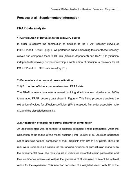
Fonseca et al., Supplementary Information FRAP data analysis

Fonseca et al., Supplementary Information 

FRAP data analysis 

1) Contribution of Diffusion to the recovery curves 

  

Fonseca, Steffen, Müller, Lu, Sawicka, Seiser and Ringrose 

In order to confirm the contribution of diffusion to the FRAP recovery curves of 

PH::GFP and PC::GFP (Fig. 4) we performed curve smoothing tests for these recovery 

curves and compared them to GFPnls (diffusion dependent) and H2A::RFP (diffusion 

independent) recovery curves confirming a contribution of diffusion to recovery for all 

PC::GFP and PH::GFP data sets (Fig. S1). 

2) Parameter extraction and cross validation 

2.1) Extraction of kinetic parameters from FRAP data 

The FRAP recovery data were analysed by fitting kinetic models (Mueller et al. 2008) 

to averaged FRAP recovery data shown in Figure 4. This fitting procedure enables the 

extraction of values for diffusion coefficient (Df), the pseudo first order association rate 

k*on and the dissociation rate koff. 

2.2) Adaptation of model for optimal parameter combination 

An additional step was performed to optimise extracted kinetic parameters. After the 

calculation of the radius of the model nucleus (RM) (Mueller et al. 2008) an additional 

set of radii was defined, composed of radii -10 pixels from RM to +20 pixels. These 30 

radii were used as input values for the reaction-diffusion or pure-difusion model fit to 

the experimental data. The resulting set of individual extracted kinetic parameters and 

their confidence intervals as well as the goodness of fit was used to select the optimal 

radius for the experiment. This selection consisted of a weighted search with 1/3 of the 

1 

  


weight being given to the goodness of the confidence intervals of association and 

dissociation constants, 1/3 to the goodness of the extracted diffusion constant 

confidence interval, 1/6 to the size of the squared sum of residuals and 1/6 to the 

distance from the initial RM, with smaller distances being favoured. MATLAB files are 

available on request. 

2.3) Contribution of binding to FRAP recovery curves 

To evaluate the role of binding in the recovery kinetics we compared reaction-diffusion 

(3 extracted parameters: Df, k*on and koff) and pure-difusion model fits (single extracted 

parameter: Df) as described in (Mueller et al. 2008) to our experimental data. In all 

cases shown in Figure 4, the best fit was given by the full reaction-diffusion model, 

indicating the presence of a bound fraction, and giving extracted values for Df, k*on and 

koff. 

2.4) Cross-validation of extracted Df 

In addition to the extracted values for Df from fitting the reaction- diffusion model, the 

Df for each protein in each cell type was measured independently. This was achieved 

by performing FRAP on the region of the metaphase cell that is outside chromatin and 

fitting the pure diffusion model (Mueller et al. 2008) to the recovery data, giving an 

independent and direct measure of Df. Interphase values were calculated by 

conversion via diffusion coefficients measured for GFP by fitting the pure diffusion 

model to FRAP recovery curves measured in both interphase and metaphase, (Table 

S1). The values of Df thus measured showed excellent agreement with those 

extracted from fitting the full model (Figure S3). 

2 

2.5) Robustness of extracted k*on, koff 

  


The robustness of the extracted k*on and koff values was examined by simulations 

performed at the value of Df that was extracted from the reaction-diffusion model fit, 

and in which k*on and koff were varied, and the fit to experimental data was evaluated 

(Fig. S4). This analysis showed that for most data sets, a limited range of k*on and koff 

values gave optimal fits to the data (Fig. S4). 

3) Other models 

3.1) Localised binding sites: metaphase 

The effect of localized binding sites in metaphase was examined using the local 

binding site model described in (Beaudouin et al. 2006; Sprague et al. 2006), showing 

that both the improved global binding (Mueller et al. 2008) and the localized binding 

(Beaudouin et al. 2006; Sprague et al. 2006) models give essentially identical results 

in conditions of low binding, as is the case for the metaphase data shown here (data 

not shown). Unlike the Müller model (Mueller et al. 2008) the Sprague model 

(Beaudouin et al. 2006; Sprague et al. 2006) does not include consideration of the 

radial bleach profile. Thus in order to achieve consistency of analysis, the Müller 

Model(Mueller et al. 2008) was used for analysis of all data sets. 

3.2) Non homogeneous distribution of proteins: interphase 

To test for the effect of non-homogeneity in protein distribution observed in interphase 

(Figure 2 and 3) on extracted kinetic parameters, we adapted the model described in 

(Mueller et al. 2008) from its original application to redistribution of photoactivatable 

3 

  


GFP, to render it applicable to the analysis of FRAP recovery curves, described here. 

Fitting this model to interphase data for individual nuclei gave similar values for the 

three extracted parameters whether initial distribution was assumed to be 

heterogenous or homogenous (Figure S2). 

3.2.1) Generation of images of single nuclei. 

In order to construct input protein distribution images for parameter extraction, all 

prebleach images of a single nucleus (250) were averaged and used to threshold the 

region of the nucleus in the total image. This region was selected to define the nucleus 

within the average image of 2s before photobleaching. Due to the speed of scanning, it 

was not feasible to image the entire nucleus. The shape of NB and SOP nuclei 

approximates well to a circle, thus the initial binding site distribution in the entire 

nucleus was reconstructed from the image of the "equatorial" region, covering 

approximately 2/3 of the nucleus. On the resulting image a circle of radius RM (model 

nucleus radius calculated as described in (Mueller et al. 2008) with adaptation as 

described in 2.1 above) was defined with the bleach region centered. This image was 

used to give the initial distribution of binding sites in the nucleus. In order to produce 

the first postbleach image, a bleach pattern with parameters describing the bleach 

spot profile was calculated from the experimental data (Mueller et al. 2008) and was 

superimposed on the prebleach image. Matlab files for image processing are available 

on request. 

3.2.2) Extraction of kinetic parameters from FRAP data, taking non 

homogeneous protein distribution into account. 

The intensity distribution images generated as described above were used as input for 

4 

  


fitting the spatial model described below to the individual FRAP recovery curve for 

each nucleus, and extraction of parameters. The spatial model was implemented in 

Mathematica (Wolfram) and is available on request. 

The reaction-diffusion system is simulated on a 2D circular domain, with a Neumann 

no-flux condition imposed on the boundary. The method-of-lines is used to numerically 

solve the resulting partial-differential equation, where a second-order finite difference 

method is used to discretize the diffusion operator on a uniform mesh. The spatial 

discretization gives rise to a coupled system of ordinary differential equations for the 

free and bound concentrations at each mesh point, which is then numerically 

integrated using an implicit solution scheme. The unknown parameters in the model 

consist of: the diffusion constant Df, the off-rate of the reaction koff, and the ratio of the 

total amount of free molecules to bound molecules, Free. Given a value for the free 

fraction, Free, the initial conditions for the free and bound proteins are obtained from 

the smoothed, pre-bleached images. Given the values of koff and Free, the spatially 

varying kon [C] is computed from the intensity distribution of the averaged chromatin 

images, following the methodology of (Mueller et al. 2008). In order to ensure the 

positivity of kon [C] in the model, a lower bound on the free fraction is imposed, whose 

value is required to be greater than the minimum chromatin intensity over its average 

for the circular domain. The unknown parameters (Df, koff, Free) are estimated from the 

measured fluorescence recovery curve for each individual nucleus by solving the 

inequality constrained optimization problem using the interior point method. As starting 

values for these three parameters, the extracted values from averaged data were used 

(Fig. 4, Table S1). 

5 

Supplementary Legends 

  


Figure S1. Diffusion influences FRAP recovery for GFPnls, PC::GFP, PH::GFP and 

H2A::RFP. Diffusion test was performed using an adaptation of the method of curve 

smoothing (Mueller et al. 2008). (A-F) Radial intensity profiles of FRAP experiments at 

four different time points after photobleaching (time in seconds is shown at the right of 

each plot). The gaussian edges of intensity profiles normalized to prebleach levels 

(Mueller et al. 2008) are plotted (symbols) and were fitted using linear regression (solid 

lines). The gray background indicates the bleach region. (A) H2A::RFP recovery is not 

affected by diffusion, indicated by similar slopes of lines at all four time points. 

Comparison of the extracted slopes was performed using ANCOVA (p-value given on 

each plot represents significance of difference between slopes at the four time points). 

(B-F) GFP-nls, PC::GFP and PH::GFP FRAP recovery shows an influence of diffusion, 

indicated by gradual flattening of radial profiles at later time points. (E) Comparative 

summary plot. For data in (A-F), the value 1/slope was calculated for each linear fit 

and normalized to the slope at time 0. These values are plotted for each data set for 

consecutive time points, showing a gradual increase in (1/slope) at later time points for 

all experiments with the exception of H2A::RFP (black) for which little change was 

detected. 

Figure S2. Comparison of the effects of binding site non-homogeneity on parameters 

extracted from FRAP experiments. Extracted diffusion (A,D,G and J), free fraction 

(B,E,H and K) and dissociation rates (koff, C,F,I and L) of PH::GFP (A-C, G-I) and 

PC::GFP (D-F, J-L) FRAP experiments in neuroblast interphase (A-F) and sensory 

organ precursor cell interphase (G-L) were analysed using an adaptation of the model 

described in (Mueller et al. 2008). (See Supplementary Information, FRAP Data 

6 

  


Analysis, for detailed description). Black bars represent the mean and 95% confidence 

intervals of the extracted parameters using the same model with an initial 

homogeneous distribution of binding sites and grey bars represent the mean and 95% 

confidence intervals of the extracted parameters using the image-based 

heterogeneous distribution of binding sites for each nucleus. n represents number of 

nuclei used in each experiment. 2-tailed paired t-tests were performed for each 

comparison resulting in p-values > 0.05 with the exception of B (p=0.0001), C 

(p=0.0069), D (p=0.0282) and E (p=0.0163). Dashed lines represent parameters 

extracted using the FRAP model described in (Mueller et al. 2008) and shown in 

Figure 4 and Table S1. 

Figure S3. Cross validation of extracted diffusion constants by independent 

measurements. (A) Comparison of diffusion constants extracted from fitting 3 

parameter FRAP model in all cell types (Df (1), black) to diffusion constants calculated 

by fitting single parameter FRAP model (diffusion only) to FRAP recovery performed 

on the non-chromatin volume in metaphase (Df (2), grey). The interphase Df values 

(grey) were calculated using GFPnls for calibration as described in Supplementary 

Information. The Df values calculated by the two procedures show good agreement. 

NB and SOP indicate neuroblast and SOP interphase and NBmet and SOPmet 

indicate neuroblast and SOP metaphase. pIIa and pIIb indicate the interphase of the 

respective cells. Data show mean of at least four measurements for each cell type. 

Error bars represent 95% confidence intervals. (B) Estimated molecular weight of 

PH::GFP and PC::GFP in neuroblasts (black) and SOPs (grey). Estimations were 

based on the extracted Df for GFPnls, PH::GFP and PC::GFP in regions outside 

chromatin at metaphase in neuroblasts and SOPs and calculated using the following 

7 

  


equation: Mwprotein = MwGFP /(Dfprotein/DfGFP)^3. The Mw estimated for PC::GFP is 

consistent with the predicted size of the PRC1 complex. In contrast, the Mw estimated 

for PH::GFP is approximately 15MDa. The PH protein has not been reported to 

participate in such large complexes, thus this result suggests that the extracted 

diffusion constant for PH::GFP may comprise both the true diffusion and a binding 

component (Mueller et al. 2008) . 

Figure S4. Parameter space for best fits of FRAP model to recovery data. For each 

FRAP recovery data set shown in Figure 4, simulations were performed in which Df 

was fixed to the value extracted from the 3 parameter fit (Fig. S3a, grey bars; Table 

S1), and k*on and koff were varied between 10 -4 and 10. For each simulation, the fit to 

the experimental data was evaluated as squared sum of residuals (ssrs). The white, 

red or black lines delineate ssrs 1.25 times larger than the minimum ssr found. Top 

row: interphase and metaphase best fit regions from each data set as indicated above 

the plots, are superimposed for comparison. Below: ssrs for each data set are plotted 

individually as heat maps (colour scale for ssrs is shown at the right of the plot.) 

Figure S5. Dot blot analysis of α-H3K27me3S28ph antibody. Serial dilutions of 

synthetic peptides corresponding to N-terminal sequence of histone H3 (amino acids 

19-37), with different S28 phosphorylation and K27 methylation status as indicated 

above the figure, were spotted on a PVDF membrane and probed with the α- 

H3K27me3S28ph antibody (dilution 1: 20000). For detection a secondary anti rabbit 

horseradish peroxidase-conjugated antibody and the Enhanced Chemiluminescence 

(ECL) detection system were used. To ensure equal peptide loading, a duplicate 

membrane was stained with Ponceau S. 

8 

  


Movie S1. PH::GFP in neuroblast. Green channel: PH::GFP under the worniu-GAL4 

driver is visualized in neuroblast and ganglion mother cells (GMCs). Red channel: 

Histone H2A::RFP is expressed under the ubiqutin promoter and visualized in all cells. 

RFP marked chromatin becomes visible in the neuroblast at mitosis. The movie starts 

at interphase; the largest cell is the neuroblast. One mitotic division up to the next 

telophase is shown. 

Movie S2. PC::GFP in neuroblast. Green channel: PC::GFP is expressed under the 

Pc promoter and is visualized in all cells. Red channel: Histone H2A::RFP is 

expressed under the ubiqutin promoter and visualized in all cells. RFP marked 

chromatin becomes visible in the neuroblast at mitosis. The movie starts at interphase; 

the largest cell is the neuroblast. One mitotic division up to the next telophase is 

shown. 

Movie S3. PH::GFP in SOP. Both PH::GFP (green channel) and histone H2A::RFP 

were expressed under the neuralized-GAL4 driver and are visible in specifically in the 

SOP and its daughter cells pIIa and pIIb. RFP marked chromatin is visible at all 

stages. The movie starts at SOP interphase. One mitotic division up to the next 

interphase is shown. At the end of the movie, the two daughter cells pIIa and pIIb are 

seen. 

Movie S4. PC::GFP in SOP. Green channel: PC::GFP is expressed under the Pc 

promoter and is visualized in all cells. Red channel: histone H2A::RFP was expressed 

under the neuralized-GAL4 driver and is visible in specifically in the SOP and its 

9 

  

Fonseca, Steffen, Müller, Lu, Sawicka, Seiser and Ringrose 10  

daughter cells pIIa and pIIb. RFP marked chromatin is visible at all stages. The movie 

starts at SOP interphase. The SOP is the largest cell and the only one showing red 

signal. One mitotic division up to the next interphase is shown. At the end of the 

movie, the two daughter cells pIIa and pIIb are seen. 

Table S1. Compilation of measured and extracted parameters of PH::GFP, PC::GFP 

and GFPnls in Neuroblast interphase (NB) and metaphase (NBmet), SOP interphase 

(SOP) and metaphase (SOPmet), pIIa interphase (pIIa) and pIIb interphase (pIIb). For 

the quantification parameters, volume measurements in cubic micrometers, 

determined by GFP fluorescence (Blue masks in Figure 2 and 3), are shown (A) as 

well as number and micromolar concentrations of GFP-fused (B, C), endogenous (D, 

E) and endogenous in yw flies (F,G) molecules of PH and PC. Kinetic parameters 

extracted using the method described in (Mueller et al. 2008) are shown in the section 

Kinetic parameters. The radius used for the parameter extraction is shown in µm (H). 

(I) represents the extracted diffusion from the full model (3 parameter fit) for PH::GFP 

and PC::GFP and from the pure diffusion model (single parameter fit) for GFPnls. (J) 

represents the extracted diffusion from the pure diffusion model in regions outside 

chromatin in NBmet and SOPmet, and the estimated PH::GFP and PC::GFP diffusions 

in interphase of all other cell types through the comparison with GFPnls diffusions 

(Fig.S3). Residence time (M) was calculated as (1/K). The fraction of bound molecules 

in the chromatin region (N) was calculated by the following equation: 100*(L)/(L+M). 

The total fraction of bound molecules (O) was calculated with the following equation: 

(N)*(T)/(B). (T) represents the number of GFP-fused proteins that are localized in the 

region determined by H2A::RFP fluorescence (Yellow masks in Figures 2 and 3). 

Number of bound GFP-fused (P), GFP-fused and endogenous (Q) and endogenous in

  

Fonseca, Steffen, Müller, Lu, Sawicka, Seiser and Ringrose 11  

yw flies (R) molecules are shown. In the Image-based parameters section are listed 

the volume in cubic micrometers occupied by chromatin (S) and the number of GFP 

proteins that are in this volume (T). As (T), (S) was determined by H2A::RFP 

fluorescence. The calculated fraction of bound molecules in the chromatin region, 

without the assumption of equilibrium, according to equation 18 of Supplementary 

Information – Mathematical modeling is listed as (U). The number of GFP-fused 

proteins bound to chromatin is listed as (W). The total fraction of bound molecules (V) 

was calculated with the ratio W/B. In the Modelling parameters section are listed the 

parameters used for the model shown in Figure 5: pseudo-first order association rate 

(X), the dissociation rate (Y) the number of endogenous Polycomb proteins (Z), as well 

as the cell (AA) and chromatin (AB) volumes. These parameters were selected from 

the experimentally determined values listed in (L), (K), (F), (A) and (S). Also shown 

are the assumed number of binding sites (AC), representing the maximum possible 

number of H3K27 methylated tails in the diploid genome based on H3K27me3 

distributions in polytene chromosomes and genome-wide ChIP profiles, assuming 

methylation of all H3 tails within a region of H3K27me3 signal. Based on this number 

of binding sites, the calculated micromolar dissociation constant (AD) is shown. 

 

184648, FigureS1, Fonseca 

A 

Normalised Intensity 

B 


C 


D 


1.2 

1.0 

0.8 

0.6 

1.0 

0.8 

0.6 

0.4 

1.0 

0.8 

0.6 

0.4 

1.0 

0.8 

0.6 

H2A::RFP - SOP 

P=0.1087 

0.5 1.0 

Radius ( m) 

1.5 

GFPnls - SOP 

P=0.0013 

1.0 1.5 

Radius ( m) 

PC::GFP - SOP 

P

NB PH 

NB PC 

SOP PH 

SOP PC 

184648, Figure S2, Fonseca 

D f (µm 2 .s -1 ) 

D f (µm 2 .s -1 ) 

D f (µm 2 .s -1 ) 

D f (µm 2 .s -1 ) 

Diffusion Free Fraction koff A B C 

5 

4 

3 

2 

1 

0 

Homogeneous Heterogeneous 

n = 5 

10 

8 

6 

4 

2 

0 

1.5 

1.0 

0.5 

0.0 

10 

8 

6 

4 

2 

0 




n = 14 

n = 6 

n = 6 

Free Fraction 

Free Fraction 

Free Fraction 

Free Fraction 

1.0 

0.8 

0.6 

0.4 

0.2 

0.0 

1.0 

0.8 

0.6 

0.4 

0.2 

0.0 

0.8 

0.6 

0.4 

0.2 

0.0 

1.0 

0.8 

0.6 

0.4 

0.2 

0.0 


D E F 


G H I 


J K L 


n = 5 

n = 14 

n = 6 

n = 6 

k off (s -1 ) 

k off (s -1 ) 

k off (s -1 ) 

k off (s -1 ) 

10 

1 

0.1 

0.01 

10 

1 

0.1 

10 

1 

0.1 

0.01 

10 

1 

0.1 

0.01 

0.001 





n = 5 

n = 14 

n = 6 

n = 6


A 

D f (µm 2 .s -1 ) 

B 

Estimated MW (kDa) 

6 

4 

2 

0 

PH NB 

PH NBmet 

100000 

10000 

1000 

100 

10 

1 

PH SOP 

Df (1) 

Df (2) 

PH SOPmet 

PH pIIa 

PH pIIb 

PC NB 

PC NBmet 

PC SOP 

PC SOPmet 

PC pIIa 

Polycomb Polyhomeotic 

PC pIIb 

NB 

SOP

184648, Figure S4, Fonseca


50 pmol 

10 pmol 

2 pmol 

Ponceau S (50 pmol) 

H3 unmodified 

H3 S28ph 

H3K27me3 

H3K27meS28ph 

H3K27me2S28ph 

H3K27me3S28ph 

H3K9me3S10ph

Section Variable ID Variable NB NBmet SOP SOPmet pIIa pIIb NB Nbmet SOP SOPmet pIIa pIIb NB Nbmet SOP SOPmet pIIa pIIb 

Image-based parameters Kinetic parameters 

Quantification 

Modeling parameters 

PH::GFP PC::GFP 

A Volume (µm 3 ) 239.55 ± 26.43 682.99 ± 97.67 149.26 ± 12.12 752.52 ± 31.53 72.71 ± 2.65 53.86 ± 4.40 176.33 ± 9.56 726.72 ± 74.88 171.60 ± 5.94 590.66 ± 37.02 97.15 ± 11.59 68.62 ± 9.76 

B # GFP 139409 ± 16220 74930 ± 8811 119147 ± 25089 133038 ± 22613 37372 ± 2367 25656 ± 2059 73350 ± 8201 118877 ± 12065 37461± 3090 39228 ± 3145 20902 ± 2222 14749 ± 1484 

C µM GFP 0.98 ± 0.06 0.19 ± 0.03 1.36 ± 0.39 0.29 ± 0.04 0.86 ± 0.02 0.80 ± 0.01 0.70 ± 0.08 0.27 ± 0.02 0.36 ± 0.02 0.11 ± 0.01 0.36 ± 0.03 0.36 ± 0.03 

D # end 24369 ± 2725 39494 ± 4008 20359 ± 1679 21320 ± 1709 11360 ± 1208 8015 ± 807 

E µM end 0.23 ± 0.03 0.09 ± 0.01 0.20 ± 0.01 0.06 ± 0.002 0.20 ± 0.01 0.20 ± 0.02 

F # end yw 40615 ± 9306 65823 ± 14762 48474 ± 13310 50762 ± 13904 27048 ± 7646 19083 ± 5355 

G µM end yw 0.38 ± 0.09 0.15 ± 0.03 0.48 ± 0.13 0.14 ± 0.04 0.48 ± 0.13 0.48 ± 0.13 

H Radius (µm) 2.27 4.38 2.86 3.43 2.28 2.28 2.99 3.45 2.91 6.36 2.37 2.19 4.19 8.18 2.91 5.52 2.78 2.80 

I Df 1 (µm 2 .s -1 ) 1.05 ± 0.17 1.26 ± 0.15 0.76 ± 0.23 1.52 ± 0.56 1.12 ± 0.31 1.11 ± 0.43 5.10 ± 0.92 2.17 ± 0.45 3.00 ± 0.34 2.43 ± 0.30 2.42 ± 0.38 2.90 ± 0.35 11.43 ± 0.96 10.50 ± 0.45 8.17 ± 0.64 9.15 ± 0.50 6.82 ± 0.72 5.77 ± 0.61 

J Df 2 (µm 2 .s -1 ) 1.14 ± 0.07 1.05 ± 0.06 0.68 ± 0.05 0.77 ± 0.06 0.57 ± 0.04 0.48 ± 0.04 3.41 ± 0.41 3.13 ± 0.38 2.80 ± 0.17 2.53 ± 0.15 2.33 ± 0.14 1.97 ± 0.12 

K k off (s -1 ) 0.23 ± 0.05 0.002 ± 0.0007 0.10 ± 0.01 0.24 ± 0.06 0.15 ± 0.01 0.13 ± 0.01 2.19 ± 0.75 0.30 ± 0.18 0.72 ± 0.40 0.002 ± 0.0007 0.24 ± 0.11 0.27 ± 0.14 

L k* on (s -1 ) 0.10 ± 0.04 0.0001 ± 0.00005 0.13 ± 0.04 0.15 ± 0.08 0.29 ± 0.05 0.27 ± 0.06 0.51 ± 0.38 0.06 ± 0.06 0.08 ± 0.08 0.0003 ± 0.00003 0.07 ± 0.04 0.04 ± 0.03 

M Rtime (s) 4.26 607.72 9.77 4.17 6.52 7.78 0.46 3.35 1.39 431.33 4.10 3.72 

N Fbound chr (%) 29.67 7.78 56.59 37.87 65.74 67.82 18.93 17.60 10.44 9.78 21.92 13.29 

O Fbound total (%) 29.67 0.41 56.59 1.81 65.74 67.82 18.93 0.53 10.44 0.94 21.92 13.29 

P # GFP bound 41360 ± 4812 310 ± 36 67421 ± 14197 2410 ± 410 24569 ± 1556 17399 ± 1396 13885 ± 1552 627 ± 64 3912 ± 321 367 ± 29 4581 ± 487 1960 ±197 

Q #GFP + end bound 18498 ± 2068 835 ± 85 6038 ± 496 566 ± 45 7070 ± 752 3026 ± 304 

R # end bound yw 7688 ± 860 347 ± 35 5062 ± 416 475 ± 38 5928 ± 630 2537 ± 255 

S Volume chr (µm 3 ) 33.24 31.58 14.15 30.59 

T # GFP chr 3,977 6,365 3,562 3,750 

U Fbound chr (%) 8.73 12.84 35.74 48.32 

V Fbound total (%) 0.46 0.61 1.07 4.62 

W # GFP chr bound 347 817 1273 1,812 

X k* 1 (s -1 ) 0.51 0.06 0.08 0.0003 0.06856 0.041193 

Y k -1 (s -1 ) 2.19 0.3 0.72 0.002 0.24429 0.26871 

Z # PC 40615 1216 48474 4633 27048 19083 

AA Volume Cell (µm3) 176.33 14.15 171.60 30.59 97.15 68.62 

AB Volume Chr (µm3) 176.33 14.15 171.60 30.59 97.15 68.62 

AC # chromatin sites 80000 80000 80000 80000 80000 80000 

AD Kd (µM) 11.23 35.04 18.28 36.67 7.71 14.13 

GFPnls

Fonseca et al., Supplementary Information FRAP data analysis

You also want an ePaper? Increase the reach of your titles

Delete template?

Save as template?