ISSUE 2007 VOLUME 2 - The World of Mathematical Equations
ISSUE 2007 VOLUME 2 - The World of Mathematical Equations
ISSUE 2007 VOLUME 2 - The World of Mathematical Equations

Create successful ePaper yourself
Turn your PDF publications into a flip-book with our unique Google optimized e-Paper software.
<strong>ISSUE</strong> <strong>2007</strong><br />
PROGRESS<br />
IN PHYSICS<br />
<strong>VOLUME</strong> 2<br />
ISSN 1555-5534
<strong>The</strong> Journal on Advanced Studies in <strong>The</strong>oretical and Experimental Physics, including Related <strong>The</strong>mes from Mathematics<br />
PROGRESS IN PHYSICS<br />
A quarterly issue scientific journal, registered with the Library <strong>of</strong> Congress (DC, USA). This journal is peer reviewed and included in the<br />
abstracting and indexing coverage <strong>of</strong>: <strong>Mathematical</strong> Reviews and MathSciNet (AMS, USA), DOAJ <strong>of</strong> Lund University (Sweden), Zentralblatt<br />
MATH (Germany), Referativnyi Zhurnal VINITI (Russia), etc.<br />
Electronic version <strong>of</strong> this journal:<br />
http://www.ptep-online.com<br />
http://www.geocities.com/ptep_online<br />
To order printed issues <strong>of</strong> this journal, contact<br />
the Editor-in-Chief.<br />
Chief Editor<br />
Dmitri Rabounski<br />
rabounski@ptep-online.com<br />
Associate Editors<br />
Florentin Smarandache<br />
smarandache@ptep-online.com<br />
Larissa Borissova<br />
borissova@ptep-online.com<br />
Stephen J. Crothers<br />
crothers@ptep-online.com<br />
Department <strong>of</strong> Mathematics and Science,<br />
University <strong>of</strong> New Mexico, 200 College<br />
Road, Gallup, NM 87301, USA<br />
Copyright c○ Progress in Physics, <strong>2007</strong><br />
All rights reserved. Any part <strong>of</strong> Progress in<br />
Physics howsoever used in other publications<br />
must include an appropriate citation<br />
<strong>of</strong> this journal.<br />
Authors <strong>of</strong> articles published in Progress in<br />
Physics retain their rights to use their own<br />
articles in any other publications and in any<br />
way they see fit.<br />
This journal is powered by LATEX<br />
A variety <strong>of</strong> books can be downloaded free<br />
from the Digital Library <strong>of</strong> Science:<br />
http://www.gallup.unm.edu/∼smarandache<br />
ISSN: 1555-5534 (print)<br />
ISSN: 1555-5615 (online)<br />
Standard Address Number: 297-5092<br />
Printed in the United States <strong>of</strong> America<br />
APRIL <strong>2007</strong> CONTENTS<br />
<strong>VOLUME</strong> 2<br />
D. Rabounski <strong>The</strong> <strong>The</strong>ory <strong>of</strong> Vortical Gravitational Fields . . . . . . . . . . . . . . . . . . . . 3<br />
L. Borissova Forces <strong>of</strong> Space Non-Holonomity as the Necessary Condition<br />
for Motion <strong>of</strong> Space Bodies. . . . . . . . . . . . . . . . . . . . . . . . . . . . . . . . . . . . . . . . . . .11<br />
H. Hu and M. Wu Evidence <strong>of</strong> Non-local Chemical, <strong>The</strong>rmal and Gravitational<br />
Effects . . . . . . . . . . . . . . . . . . . . . . . . . . . . . . . . . . . . . . . . . . . . . . . . . . . . . . . . 17<br />
S. J. Crothers On Line-Elements and Radii: A Correction . . . . . . . . . . . . . . . . . . . 25<br />
S. J. Crothers Relativistic Cosmology Revisited . . . . . . . . . . . . . . . . . . . . . . . . . . . . 27<br />
F. Potter and H. G. Preston Cosmological Redshift Interpreted as Gravitational<br />
Redshift. . . . . . . . . . . . . . . . . . . . . . . . . . . . . . . . . . . . . . . . . . . . . . . . . . . . . . .31<br />
R. Pérez-Enríquez, J. L. Marín and R. Riera Exact Solution <strong>of</strong> the Three-<br />
Body Santilli-Shillady Model <strong>of</strong> the Hydrogen Molecule . . . . . . . . . . . . . . . . 34<br />
W. Tawfik Study <strong>of</strong> the Matrix Effect on the Plasma Characterization <strong>of</strong> Six<br />
Elements in Aluminum Alloys using LIBS With a Portable Echelle Spectrometer<br />
. . . . . . . . . . . . . . . . . . . . . . . . . . . . . . . . . . . . . . . . . . . . . . . . . . . . . . . . . . . . 42<br />
A Letter by the Editor-in-Chief: Twenty-Year Anniversary <strong>of</strong> the Orthopositronium<br />
Lifetime Anomalies: <strong>The</strong> Puzzle Remains Unresolved. . . . . . . . . . .50<br />
B. M. Levin A Proposed Experimentum Crucis for the Orthopositronium Lifetime<br />
Anomalies. . . . . . . . . . . . . . . . . . . . . . . . . . . . . . . . . . . . . . . . . . . . . . . . . . . . . .53<br />
V. Christianto, D. L. Rapoport and F. Smarandache Numerical Solution <strong>of</strong><br />
Time-Dependent Gravitational Schrödinger Equation . . . . . . . . . . . . . . . . . . . 56<br />
V. Christianto and F. Smarandache A Note on Unified Statistics Including<br />
Fermi-Dirac, Bose-Einstein, and Tsallis Statistics, and Plausible Extension<br />
to Anisotropic Effect . . . . . . . . . . . . . . . . . . . . . . . . . . . . . . . . . . . . . . . . . . . . . . . . . 61<br />
R. Rajamohan and A. Satya Narayanan On the Rate <strong>of</strong> Change <strong>of</strong> Period<br />
for Accelerated Motion and <strong>The</strong>ir Implications in Astrophysics . . . . . . . . . . 65<br />
S. J. Crothers Gravitation on a Spherically Symmetric Metric Manifold . . . . . . 68<br />
N. Stavroulakis On the Propagation <strong>of</strong> Gravitation from a Pulsating Source . . . 75<br />
A. Khazan Effect from Hyperbolic Law in Periodic Table <strong>of</strong> Elements . . . . . . . 83<br />
W. Tawfik Fast LIBS Identification <strong>of</strong> Aluminum Alloys . . . . . . . . . . . . . . . . . . . . 87<br />
A. Yefremov Notes on Pioneer Anomaly Explanation by Sattellite-Shift Formula<br />
<strong>of</strong> Quaternion Relativity: Remarks on “Less Mundane Explanation<br />
<strong>of</strong> Pioneer Anomaly from Q-Relativity” . . . . . . . . . . . . . . . . . . . . . . . . . . . . . . . 93<br />
D. D. Georgiev Single Photon Experiments and Quantum Complementarity . . . 97<br />
A. Khazan Upper Limit <strong>of</strong> the Periodic Table and Synthesis <strong>of</strong> Superheavy<br />
Elements. . . . . . . . . . . . . . . . . . . . . . . . . . . . . . . . . . . . . . . . . . . . . . . . . . . . . . . . . . .104
Information for Authors and Subscribers<br />
Progress in Physics has been created for publications on advanced studies<br />
in theoretical and experimental physics, including related themes from<br />
mathematics. All submitted papers should be pr<strong>of</strong>essional, in good English,<br />
containing a brief review <strong>of</strong> a problem and obtained results.<br />
All submissions should be designed in L ATEX format using Progress<br />
in Physics template. This template can be downloaded from Progress in<br />
Physics home page http://www.ptep-online.com. Abstract and the necessary<br />
information about author(s) should be included into the papers. To submit a<br />
paper, mail the file(s) to Chief Editor.<br />
All submitted papers should be as brief as possible. Commencing 1st<br />
January 2006 we accept brief papers, no larger than 8 typeset journal pages.<br />
Short articles are preferable. Papers larger than 8 pages can be considered<br />
in exceptional cases to the section Special Reports intended for such publications<br />
in the journal.<br />
All that has been accepted for the online issue <strong>of</strong> Progress in Physics is<br />
printed in the paper version <strong>of</strong> the journal. To order printed issues, contact<br />
Chief Editor.<br />
This journal is non-commercial, academic edition. It is printed from<br />
private donations.
April, <strong>2007</strong> PROGRESS IN PHYSICS Volume 2<br />
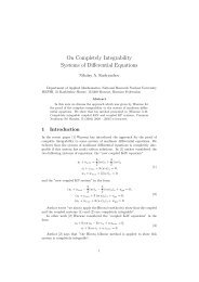
1 <strong>The</strong> mathematical method<br />
<strong>The</strong> <strong>The</strong>ory <strong>of</strong> Vortical Gravitational Fields<br />
Dmitri Rabounski<br />
E-mail: rabounski@yahoo.com<br />
This paper treats <strong>of</strong> vortical gravitational fields, a tensor <strong>of</strong> which is the rotor <strong>of</strong><br />
the general covariant gravitational inertial force. <strong>The</strong> field equations for a vortical<br />
gravitational field (the Lorentz condition, the Maxwell-like equations, and the<br />
continuity equation) are deduced in an analogous fashion to electrodynamics. From<br />
the equations it is concluded that the main kind <strong>of</strong> vortical gravitational fields is<br />
“electric”, determined by the non-stationarity <strong>of</strong> the acting gravitational inertial force.<br />
Such a field is a medium for traveling waves <strong>of</strong> the force (they are different to the<br />
weak deformation waves <strong>of</strong> the space metric considered in the theory <strong>of</strong> gravitational<br />
waves). Standing waves <strong>of</strong> the gravitational inertial force and their medium, a vortical<br />
gravitational field <strong>of</strong> the “magnetic” kind, are exotic, since a non-stationary rotation <strong>of</strong><br />
a space body (the source <strong>of</strong> such a field) is a very rare phenomenon in the Universe.<br />
<strong>The</strong>re are currently two methods for deducing a formula for<br />
the Newtonian gravitational force in General Relativity. <strong>The</strong><br />
first method, introduced by Albert Einstein himself, has its<br />
basis in an arbitrary interpretation <strong>of</strong> Christ<strong>of</strong>fel’s symbols<br />
in the general covariant geodesic equations (the equation <strong>of</strong><br />
motion <strong>of</strong> a free particle) in order to obtain a formula like<br />
that by Newton (see [1], for instance). <strong>The</strong> second method is<br />
due to Abraham Zelmanov, who developed it in the 1940’s<br />
[2, 3]. This method determines the gravitational force in<br />
an exact mathematical way, without any suppositions, as<br />
a part <strong>of</strong> the gravitational inertial force derived from the<br />
non-commutativity <strong>of</strong> the differential operators invariant in<br />
an observer’s spatial section. This formula results from Zelmanov’s<br />
mathematical apparatus <strong>of</strong> chronometric invariants<br />
(physical observable quantities in General Relativity).<br />
<strong>The</strong> essence <strong>of</strong> Zelmanov’s mathematical apparatus [4]<br />
is that if an observer accompanies his reference body, his<br />
observable quantities are the projections <strong>of</strong> four-dimensional<br />
quantities upon his time line and the spatial section — chronometrically<br />
invariant quantities, via the projecting operators<br />
b α = dxα<br />
ds and hαβ = −gαβ + bαbβ, which fully define his<br />
real reference space (here b α is his velocity relative to his<br />
real references). So the chr.inv.-projections <strong>of</strong> a world-vector<br />
Q α are bαQ α = Q0<br />
√ g00 and hi αQ α = Q i , while the chr.inv.-<br />
projections <strong>of</strong> a 2nd rank world-tensor Q αβ are b α b β Qαβ =<br />
= Q00<br />
g00 , hiαbβ Qαβ = Qi<br />
√ 0 , h g00 i αhk βQαβ = Qik . <strong>The</strong> principal<br />
physical observable properties <strong>of</strong> a space are derived from<br />
the fact that the chr.inv.-differential operators ∗ ∂<br />
and ∗ ∂<br />
∂x i = ∂<br />
∂x i + 1<br />
− ∗ ∂ 2<br />
∂t ∂xi = 1<br />
c2 ∗<br />
∂<br />
Fi<br />
c2 ∗<br />
∂<br />
vi ∂t<br />
∂t and<br />
∂t<br />
are non-commutative as<br />
∗ 2<br />
∂<br />
∂xi∂x k − ∗ ∂ 2<br />
∂xk∂x i = 2<br />
c2 Aik ∂t<br />
1 = √<br />
∂<br />
g00 ∂t<br />
∗ 2<br />
∂<br />
∂xi∂t −<br />
∗<br />
∂<br />
, and<br />
also that the chr.inv.-metric tensor hik =−gik + bi bk may<br />
not be stationary. <strong>The</strong> principal physical observable characteristics<br />
are the chr.inv.-vector <strong>of</strong> the gravitational inertial<br />
force Fi, the chr.inv.-tensor <strong>of</strong> the angular velocities <strong>of</strong> the<br />
space rotation Aik, and the chr.inv.-tensor <strong>of</strong> the rates <strong>of</strong> the<br />
space deformations Dik:<br />
Fi = 1<br />
√ g00<br />
�<br />
∂w ∂vi<br />
−<br />
∂xi ∂t<br />
Aik = 1<br />
�<br />
∂vk ∂vi<br />
−<br />
2 ∂xi ∂xk Dik = 1 ∗∂hik 2 ∂t<br />
�<br />
, w = c 2 (1 − √ g00) , (1)<br />
�<br />
+ 1<br />
2c 2 (Fivk − Fkvi) , (2)<br />
, D ik =− 1 ∗ ik ∂h<br />
, D =D<br />
2 ∂t<br />
k √<br />
∗∂ ln h<br />
k = , (3)<br />
∂t<br />
c g0i<br />
where w is the gravitational potential, vi =− √ is the<br />
g00<br />
linear velocity <strong>of</strong> the space rotation, hik = −gik + 1<br />
c2 vivk<br />
is the chr.inv.-metric tensor, h= det�hik�, hg00 =−g, and<br />
g = det�gαβ�. <strong>The</strong> observable non-uniformity <strong>of</strong> the space<br />
is set up by the chr.inv.-Christ<strong>of</strong>fel symbols<br />
Δ i jk = h im Δjk,m = 1<br />
2 him<br />
� ∗∂hjm<br />
+<br />
∂xk ∗∂hkm −<br />
∂xj ∗∂hjk ∂xm �<br />
, (4)<br />
which are constructed just like Christ<strong>of</strong>fel’s usual symbols<br />
Γ α μν = g ασ Γμν,σ using hik instead <strong>of</strong> gαβ.<br />
A four-dimensional generalization <strong>of</strong> the chr.inv.-quantities<br />
Fi, Aik, and Dik is [5]<br />
where<br />
Fα = −2c 2 b β aβα , (5)<br />
Aαβ = ch μ αh ν β aμν , (6)<br />
Dαβ = ch μ αh ν β dμν , (7)<br />
aαβ = 1<br />
2 (∇α bβ −∇β bα) , dαβ = 1<br />
2 (∇α bβ +∇β bα) . (8)<br />
For instance, the chr.inv.-projections <strong>of</strong> F α are<br />
ϕ = bαF α = F0<br />
√g00<br />
= 0 , q i = h i αF α = F i . (9)<br />
D. Rabounski. <strong>The</strong> <strong>The</strong>ory <strong>of</strong> Vortical Gravitational Fields 3
Volume 2 PROGRESS IN PHYSICS April, <strong>2007</strong><br />
Proceeding from the exact formula for the gravitational<br />
inertial force above, we can, for the first time, determine<br />
vortical gravitational fields.<br />
2 D’Alembert’s equations <strong>of</strong> the force<br />
It is a matter <strong>of</strong> fact that two bodies attract each other due<br />
to the transfer <strong>of</strong> the force <strong>of</strong> gravity. <strong>The</strong> force <strong>of</strong> gravity<br />
is absent in a homogeneous gravitational field, because the<br />
gradient <strong>of</strong> the gravitational potential w is zero everywhere<br />
therein. <strong>The</strong>refore it is reasonable to consider the field <strong>of</strong> the<br />
vector potential F α as a medium transferring gravitational<br />
attraction via waves <strong>of</strong> the force.<br />
D’Alembert’s equations <strong>of</strong> the vector field F α without<br />
its inducing sources<br />
F α = 0 (10)<br />
are the equations <strong>of</strong> propagation <strong>of</strong> waves traveling in the<br />
field ∗ . <strong>The</strong> equations have two chr.inv.-projections<br />
which are the same as<br />
bσ F σ = 0 , h i σ F σ = 0 , (11)<br />
bσ g αβ ∇α∇β F σ = 0 , h i σ g αβ ∇α∇β F σ = 0 . (12)<br />
<strong>The</strong>se are the chr.inv.-d’Alembert equations for the field<br />
F α = −2c 2 a ∙α σ∙b σ without its-inducing sources. To obtain the<br />
equations in detailed form isn’t an easy process. Helpful<br />
here is the fact that the chr.inv.-projection <strong>of</strong> F α upon a<br />
time line is zero. Following this path, after some algebra,<br />
we obtain the chr.inv.-d’Alembert equations (11) in the final<br />
form<br />
1<br />
c2 ∗<br />
∂<br />
∂t<br />
� k<br />
FkF � + 1<br />
∗ i<br />
∂F<br />
Fi<br />
c2 ∂t + Dk ∗ m<br />
∂F<br />
m +<br />
∂xk + h ik ∗ ∂<br />
∂x i [(Dkn + Akn)F n ] − 2<br />
c 2 AikF i F k +<br />
+ 1<br />
c 2 FmF m D + Δ m knD k mF n −<br />
− h ik Δ m ik (Dmn + Amn) F n = 0 ,<br />
1<br />
+ m c2 � i<br />
Dk + A ∙i �<br />
k∙<br />
∗ ∂F k<br />
∂t +<br />
+ 1<br />
c2 ∗<br />
∂ �� i<br />
Dk +A<br />
∂t<br />
∙i � k<br />
k∙ F � + 1<br />
∗ i<br />
∂F 1<br />
D +<br />
c2 ∂t c2 F k ∗ ∂F i<br />
+<br />
∂xk + 1<br />
c2 � i<br />
Dn +A ∙i � n 1<br />
n∙ F D −<br />
c2 ΔikmF k F m + 1<br />
c4 FkF k F i −<br />
− h km<br />
�<br />
∗∂<br />
∂xk � i<br />
ΔmnF n� + � Δ i knΔ n mp −Δ n kmΔ i � p<br />
np F +<br />
+ Δ i ∗ n<br />
∂F<br />
kn<br />
∂xm − Δn ∗ i<br />
∂F<br />
km<br />
∂xn ⎪⎬<br />
(13)<br />
�<br />
= 0 .<br />
⎪⎭<br />
1<br />
c2 ∗ 2 i<br />
∂ F<br />
∂t2 − hkm ∗ ∂ 2 F i<br />
∂xk∂x ∗ <strong>The</strong> waves travelling in the field <strong>of</strong> the gravitational inertial force<br />
aren’t the same as the waves <strong>of</strong> the weak perturbations <strong>of</strong> the space metric,<br />
routinely considered in the theory <strong>of</strong> gravitational waves.<br />
⎫<br />
3 A vortical gravitational field. <strong>The</strong> field tensor and<br />
pseudo-tensor. <strong>The</strong> field invariants<br />
We introduce the tensor <strong>of</strong> the field as a rotor <strong>of</strong> its fourdimensional<br />
vector potential F α as well as Maxwell’s tensor<br />
<strong>of</strong> electromagnetic fields, namely<br />
Fαβ = ∇α Fβ − ∇β Fα = ∂Fβ<br />
∂x<br />
∂Fα<br />
− . (14)<br />
α ∂xβ We will refer to Fαβ (14) as the tensor <strong>of</strong> a vortical<br />
gravitational field, because this is actual a four-dimensional<br />
vortex <strong>of</strong> an acting gravitational inertial force F α .<br />
Taking into account that the chr.inv.-projections <strong>of</strong> the<br />
field potential F α =−2c 2 a ∙α σ∙b σ are<br />
F0 √ = 0, F g00 i = hikFk, we obtain the components <strong>of</strong> the field tensor Fαβ:<br />
F00 = F 00 = 0 , F0i = − 1 √<br />
g00<br />
Fik =<br />
F ∙0<br />
0∙ = 1<br />
F ∙0<br />
k∙ = 1<br />
√ g00<br />
∗ ∗ ∂Fi ∂Fk 1<br />
− +<br />
∂xk ∂xi c2 � ∗∂Fk vi − vk<br />
∂t<br />
c2 vk ∗∂Fk ∂t<br />
c<br />
, F ∙i<br />
0∙ = 1<br />
c<br />
� ∗ 1 ∂Fk 1<br />
−<br />
c ∂t<br />
F ∙i<br />
k∙ = h im<br />
� ∗∂Fm<br />
−<br />
∂xk F 0k = 1<br />
�<br />
1<br />
√<br />
g00 c hkm ∗∂Fm F ik = h im h kn<br />
� ∗∂Fm<br />
−<br />
∂xn c 3 vkv m ∗ ∂Fm<br />
∗ ∂Fi<br />
∂t<br />
∗ ∂Fi<br />
∂t<br />
, (15)<br />
�<br />
, (16)<br />
√<br />
g00 h ik ∗∂Fk , (17)<br />
∂t<br />
∂t +<br />
+ 1<br />
c vm<br />
�∗∂Fm ∗∂Fk −<br />
∂xk ∂xm ��<br />
,<br />
(18)<br />
∗∂Fk ∂xm �<br />
− 1<br />
c2 him ∗∂Fm vk ,<br />
∂t<br />
(19)<br />
∂t +<br />
+ 1<br />
c vnh mk<br />
� ∗∂Fn ∗∂Fm −<br />
∂xm ∂xn ��<br />
,<br />
(20)<br />
∗∂Fn ∂xm �<br />
. (21)<br />
We see here two chr.inv.-projections <strong>of</strong> the field tensor<br />
Fαβ. We will refer to the time projection<br />
E i =<br />
∙i F0∙ √ =<br />
g00<br />
1<br />
c hik ∗∂Fk ∂t<br />
, Ei = hikE k = 1 ∗∂Fi c ∂t<br />
(22)<br />
as the “electric” observable component <strong>of</strong> the vortical gravitational<br />
field, while the spatial projection will be referred to<br />
as the “magnetic” observable component <strong>of</strong> the field<br />
H ik = F ik = h im h kn<br />
� ∗∂Fm<br />
−<br />
∂xn Hik = himhknH mn =<br />
∗ ∂Fn<br />
∂x m<br />
�<br />
, (23)<br />
∗ ∗ ∂Fi ∂Fk<br />
−<br />
∂xk ∂xi , (24)<br />
4 D. Rabounski. <strong>The</strong> <strong>The</strong>ory <strong>of</strong> Vortical Gravitational Fields
April, <strong>2007</strong> PROGRESS IN PHYSICS Volume 2<br />
which, after use <strong>of</strong> the 1st Zelmanov identity [2, 3] that<br />
links the spatial vortex <strong>of</strong> the gravitational inertial force to<br />
the non-stationary rotation <strong>of</strong> the observer’s space<br />
� ∗ ∗∂Fk ∗<br />
∂Aik 1 ∂Fi<br />
+ −<br />
∂t 2 ∂xi ∂xk �<br />
= 0 , (25)<br />
takes the form<br />
H ik = 2h im h kn ∗ ∂Amn<br />
∂t<br />
∗∂Aik , Hik = 2 . (26)<br />
∂t<br />
<strong>The</strong> “electric” observable component E i <strong>of</strong> a vortical<br />
gravitational field manifests as the non-stationarity <strong>of</strong> the<br />
acting gravitational inertial force F i . <strong>The</strong> “magnetic” observable<br />
component Hik manifests as the presence <strong>of</strong> the<br />
spatial vortices <strong>of</strong> the force F i or equivalently, as the nonstationarity<br />
<strong>of</strong> the space rotation Aik (see formula 26). Thus,<br />
two kinds <strong>of</strong> vortical gravitational fields are possible:<br />
1. Vortical gravitational fields <strong>of</strong> the “electric” kind<br />
(Hik = 0, E i �= 0). In this field we have no spatial<br />
vortices <strong>of</strong> the acting gravitational inertial force F i ,<br />
which is the same as a stationary space rotation. So a<br />
vortical field <strong>of</strong> this kind consists <strong>of</strong> only the “electric”<br />
component E i (22) that is the non-stationarity <strong>of</strong> the<br />
force F i . Note that a vortical gravitational field <strong>of</strong> the<br />
“electric” kind is permitted in both a non-holonomic<br />
(rotating) space, if its rotation is stationary, and also<br />
in a holonomic space since the zero rotation is the<br />
ultimate case <strong>of</strong> stationary rotations;<br />
2. <strong>The</strong> “magnetic” kind <strong>of</strong> vortical gravitational fields is<br />
characterized by E i = 0 and Hik �= 0. Such a vortical<br />
field consists <strong>of</strong> only the “magnetic” components Hik,<br />
which are the spatial vortices <strong>of</strong> the acting force F i<br />
and the non-stationary rotation <strong>of</strong> the space. <strong>The</strong>refore<br />
a vortical gravitational field <strong>of</strong> the “magnetic” kind is<br />
permitted only in a non-holonomic space. Because the<br />
d’Alembert equations (13), with the condition E i = 0,<br />
don’t depend on time, a “magnetic” vortical gravitational<br />
field is a medium for standing waves <strong>of</strong> the<br />
gravitational inertial force.<br />
In addition, we introduce the pseudotensor F ∗αβ <strong>of</strong> the<br />
field dual to the field tensor<br />
F ∗αβ = 1<br />
2 Eαβμν Fμν , F∗αβ = 1<br />
2 EαβμνF μν , (27)<br />
where the four-dimensional completely antisymmetric dis-<br />
√<br />
−g<br />
criminant tensors Eαβμν = eαβμν √ and Eαβμν = eαβμν<br />
−g<br />
transform tensors into pseudotensors in the inhomogeneous<br />
anisotropic four-dimensional pseudo-Riemannian space∗ .<br />
Using the components <strong>of</strong> the field tensor Fαβ, we obtain<br />
∗ Here e αβμν and eαβμν are Levi-Civita’s unit tensors: the fourdimensional<br />
completely antisymmetric unit tensors which transform tensors<br />
into pseudotensors in a Galilean reference frame in the four-dimensional<br />
pseudo-Euclidean space [1].<br />
the chr.inv.-projections <strong>of</strong> the field pseudotensor F ∗αβ :<br />
H ∗i =<br />
� ∗∂Fk ∗∂Fm −<br />
∂xm ∂xk �<br />
, (28)<br />
∗∙i F0∙ √ =<br />
g00<br />
1<br />
2 εikm<br />
E ∗ik = F ∗ik = − 1<br />
c εikm ∗∂Fm , (29)<br />
∂t<br />
where εikm = b0 E0ikm = √ g00 E0ikm = eikm √ and εikm =<br />
h<br />
= b0E0ikm = E0ikm<br />
√<br />
√ = eikm h are the chr.inv.-discriminant<br />
g00<br />
tensors [2]. Taking into account the 1st Zelmanov identity<br />
(25) and the formulae for differentiating εikm and εikm [2]<br />
∗ ∂εimn<br />
∂t = εimn D ,<br />
∗ ∂ε imn<br />
∂t = −εimn D , (30)<br />
we write the “magnetic” component H∗i as follows<br />
H ∗i = ε ikm ∗ � ∗∂Ω∗i ∂Akm<br />
= 2<br />
∂t ∂t + Ω∗i �<br />
D , (31)<br />
where Ω ∗i = 1<br />
2 εikm Akm is the chr.inv.-pseudovector <strong>of</strong> the<br />
angular velocity <strong>of</strong> the space rotation, while the trace D =<br />
= h ik Dik = D n n <strong>of</strong> the tensor Dik is the rate <strong>of</strong> the relative<br />
expansion <strong>of</strong> an elementary volume permeated by the field.<br />
Calculating the invariants <strong>of</strong> a vortical gravitational field<br />
(J1 = Fαβ F αβ and J2 = Fαβ F ∗αβ ), we obtain<br />
J1 =h im h kn<br />
�∗∂Fi −<br />
∂xk ∗ ∂Fk<br />
∂x i<br />
J2 = − 2<br />
c εimn<br />
� ∗∂Fm<br />
−<br />
∂xn ��∗∂Fm −<br />
∂xn − 2<br />
c2 hik ∗∂Fi ∂t<br />
∗ ∂Fn<br />
∂x m<br />
which, with the 1st Zelmanov identity (25), are<br />
J1 = 4h im h kn ∗ ∂Aik<br />
∂t<br />
∗ ∂Amn<br />
∂t<br />
J2 = − 4<br />
c εimn ∗ ∗<br />
∂Amn ∂Fi<br />
∂t<br />
∗∂Fn ∂xm �<br />
−<br />
∗∂Fk ,<br />
∂t<br />
(32)<br />
� ∗∂Fi<br />
,<br />
∂t<br />
(33)<br />
2<br />
−<br />
c2 hik ∗ ∗ ∂Fi ∂Fk<br />
, (34)<br />
∂t ∂t<br />
∂t =<br />
= − 8<br />
� ∗∂Ω∗i c ∂t + Ω∗i � ∗∂Fi<br />
D .<br />
∂t<br />
(35)<br />
By the strong physical condition <strong>of</strong> isotropy, a field is<br />
isotropic if both invariants <strong>of</strong> the field are zeroes: J1 = 0<br />
means that the lengths <strong>of</strong> the “electric” and the “magnetic”<br />
components <strong>of</strong> the field are the same, while J2 = 0 means<br />
that the components are orthogonal to each other. Owning<br />
the case <strong>of</strong> a vortical gravitational field, we see that such a<br />
field is isotropic if the common conditions are true<br />
h im h kn ∗ ∂Aik<br />
∂t<br />
∗ ∂Amn<br />
∂t<br />
∗ ∂Fi<br />
∂t<br />
∗ ∂Amn<br />
∂t<br />
= 0<br />
1<br />
=<br />
2c2 hik ∗ ∗ ∂Fi ∂Fk<br />
∂t ∂t<br />
D. Rabounski. <strong>The</strong> <strong>The</strong>ory <strong>of</strong> Vortical Gravitational Fields 5<br />
⎫<br />
⎪⎬<br />
⎪⎭<br />
(36)
Volume 2 PROGRESS IN PHYSICS April, <strong>2007</strong><br />
however their geometrical sense is not clear.<br />
Thus the anisotropic field can only be a mixed vortical<br />
gravitational field bearing both the “electric” and the “magnetic”<br />
components. A strictly “electric” or “magnetic” vortical<br />
gravitational field is always spatially isotropic.<br />
Taking the above into account, we arrive at the necessary<br />
and sufficient conditions for the existence <strong>of</strong> standing waves<br />
<strong>of</strong> the gravitational inertial force:<br />
1. A vortical gravitational field <strong>of</strong> the strictly “magnetic”<br />
kind is the medium for standing waves <strong>of</strong> the gravitational<br />
inertial force;<br />
2. Standing waves <strong>of</strong> the gravitational inertial force are<br />
permitted only in a non-stationary rotating space.<br />
As soon as one <strong>of</strong> the conditions ceases, the acting gravitational<br />
inertial force changes: the standing waves <strong>of</strong> the<br />
force transform into traveling waves.<br />
4 <strong>The</strong> field equations <strong>of</strong> a vortical gravitational field<br />
It is known from the theory <strong>of</strong> fields that the field equations<br />
<strong>of</strong> a field <strong>of</strong> a four-dimensional vector-potential A α is a<br />
system consisting <strong>of</strong> 10 equations in 10 unknowns:<br />
• Lorentz’s condition ∇σA σ = 0 states that the fourdimensional<br />
potential A α remains unchanged;<br />
• the continuity equation ∇σ jσ = 0 states that the fieldinducing<br />
sources (“charges” and “currents”) can not<br />
be destroyed but merely re-distributed in the space;<br />
• two groups (∇σF ασ = 4π<br />
c jα and ∇σF ∗ασ = 0) <strong>of</strong> the<br />
Maxwell-like equations, where the 1st group determines<br />
the “charge” and the “current” as the components<br />
<strong>of</strong> the four-dimensional current vector jα <strong>of</strong> the field.<br />
This system completely determines a vector field A α and<br />
its sources in a pseudo-Riemannian space. We shall deduce<br />
the field equations for a vortical gravitational field as a field<br />
To deduce the Maxwell-like equations for a vortical gravitational<br />
field, we collect together the chr.inv.-projections<br />
<strong>of</strong> the field tensor Fαβ and the field pseudotensor F ∗αβ . Expressing<br />
the necessary projections with the tensor <strong>of</strong> the rate<br />
<strong>of</strong> the space deformation D ik to eliminate the free h ik terms,<br />
we obtain<br />
E i = 1<br />
c hik ∗∂Fk ∂t<br />
H ik = 2h im h kn ∗ ∂Amn<br />
∗ i 1 ∂F 2<br />
= +<br />
c ∂t c Fk D ik , (39)<br />
∂t =<br />
∗ ik ∂A<br />
= 2<br />
∂t + 4 � A i∙<br />
∙nD kn − A k∙<br />
∙mD im� ,<br />
H ∗i = ε imn ∗ ∂Amn<br />
∂t<br />
(40)<br />
∗ ∗i ∂Ω<br />
= 2<br />
∂t + 2Ω∗iD , (41)<br />
E ∗ik = − 1<br />
c εikm ∗∂Fm . (42)<br />
∂t<br />
After some algebra, we obtain the chr.inv.-Maxwell-like<br />
equations for a vortical gravitational field<br />
∗ 2 i<br />
1 ∂ F<br />
c ∂xi ∗<br />
2 ∂<br />
+<br />
∂t c ∂xi �<br />
FkD ik� + 1<br />
�<br />
∗∂F<br />
�<br />
i<br />
ik<br />
+2FkD Δ<br />
c ∂t j<br />
ji− − 2<br />
c Aik<br />
�<br />
∗∂Aik ∂t +Ai∙ ∙nD kn<br />
�<br />
= 4πρ<br />
∗ 2 ik<br />
∂ A<br />
2<br />
∂xk 1<br />
−<br />
∂t c2 ∗ 2 i ∗<br />
∂ F ∂<br />
+4<br />
∂t2 ∂xk � i∙<br />
A∙nD kn −A k∙<br />
∙mD im� +<br />
�<br />
+2 Δ j<br />
�<br />
1<br />
jk− Fk<br />
c2 � ∗ ik<br />
∂A<br />
∂t +2�A i∙<br />
∙nD kn −A k∙<br />
∙mD im��<br />
−<br />
− 2<br />
c2 ∗<br />
∂ � ik<br />
FkD<br />
∂t<br />
� − 1<br />
c2 �<br />
∗∂F i<br />
∂t +2FkDik<br />
�<br />
D = 4π<br />
c ji<br />
⎫<br />
⎪⎬<br />
(43)<br />
⎪⎭<br />
⎫<br />
∗ 2 ∗i<br />
∂ Ω<br />
∂xi∂t +<br />
∗<br />
∂<br />
∂xi � � ∗i 1<br />
Ω D +<br />
c2 Ω∗m ∗ ∂Fm<br />
+<br />
ε ikm ∗ ∂ 2 Fm<br />
∂xk �<br />
+ εikm Δ<br />
∂t j<br />
jk<br />
� ∗∂Ω ∗i<br />
∗ ∗i<br />
∂Ω<br />
+ 4D<br />
∂t +2<br />
∂t + Ω∗i D<br />
� ∗<br />
1 ∂Fm<br />
− Fk<br />
c2 ∂t +2<br />
∂t +<br />
�<br />
Δ j<br />
ji<br />
∗ ∂ 2 Ω ∗i<br />
Group I,<br />
= 0 ⎪⎬<br />
Group II.<br />
∂t2 +<br />
�<br />
∗∂D<br />
∂t +D2<br />
�<br />
Ω ∗i = 0 ⎪⎭<br />
<strong>of</strong> the four-dimensional potential F α = −2c2a∙α σ∙bσ .<br />
Writing the divergence ∇σF σ σ<br />
∂F =<br />
∂xσ + Γσ σμF μ chr.inv.-form [2, 3]<br />
in the<br />
∇σF σ = 1<br />
� ∗∂ϕ<br />
c ∂t +ϕD<br />
� ∗ i ∂q<br />
+<br />
∂xi +qi ∗∂ln √ h<br />
∂xi 1<br />
−<br />
c2 Fiq i (37)<br />
where ∗ ∂ ln √ h<br />
∂xi = Δ j<br />
ji and ∗ ∂q i<br />
∂xi + qiΔ j<br />
ji =∗∇i qi , we obtain<br />
the chr.inv.-Lorentz condition in a vortical gravitational field<br />
∗ i ∂F<br />
∂xi + F i Δ j 1<br />
ji −<br />
c2 FiF i <strong>The</strong> chr.inv.-continuity equation ∇σj<br />
= 0 . (38)<br />
σ = 0 for a vortical<br />
gravitational field follows from the 1st group <strong>of</strong> the Maxwelllike<br />
equations, and is<br />
∗ 2<br />
∂<br />
∂xi∂x k<br />
�<br />
∗∂A<br />
�<br />
ik<br />
−<br />
∂t<br />
1<br />
c2 �<br />
∗∂Aik ∂t +Ai∙ ∙nD kn<br />
�� �<br />
∗<br />
∂Aik<br />
AikD+ −<br />
∂t<br />
− 1<br />
c2 �<br />
∗∂2 ik<br />
A<br />
∂t2 +<br />
∗<br />
∂�<br />
i∙<br />
A∙nD ∂t<br />
nk��<br />
Aik+ 1<br />
2c2 �<br />
∗∂F i<br />
∂t +2FkDik<br />
�<br />
×<br />
�∗∂Δj ∗<br />
ji D ∂D<br />
× + Fi−<br />
∂t c2 ∂xi �<br />
∗ 2<br />
∂<br />
+2<br />
∂xi∂x k<br />
� i∙<br />
A∙nD kn −A k∙<br />
∙mD im� +<br />
�<br />
∗∂Aik +<br />
∂t +2�A i∙<br />
∙nD kn −A k∙<br />
∙mD im��� ∗<br />
∂<br />
∂xi �<br />
Δ j<br />
�<br />
1<br />
jk− Fk +<br />
c2 �<br />
+ Δ j<br />
��<br />
1<br />
ji − Fi Δ<br />
c2 l lk − 1<br />
�<br />
Fk<br />
c2 �<br />
(45)<br />
= 0 .<br />
(44)<br />
To see a simpler sense <strong>of</strong> the obtained field equations, we<br />
take the field equations in a homogeneous space (Δi km = 0)<br />
6 D. Rabounski. <strong>The</strong> <strong>The</strong>ory <strong>of</strong> Vortical Gravitational Fields
April, <strong>2007</strong> PROGRESS IN PHYSICS Volume 2<br />
free <strong>of</strong> deformation (Dik = 0) ∗ . In such a space the chr.inv.-<br />
Maxwell-like equations obtained take the simplified form<br />
∗ 2 i 1 ∂ F<br />
c ∂xi 2<br />
−<br />
∂t c Aik<br />
∗ ik ∂A<br />
∂t<br />
∗ 2 ik ∂ A<br />
2<br />
∂xk∂t ∗ ∂ 2 Ω ∗i<br />
∂x i ∂t<br />
ε ikm ∗ ∂ 2 Fm<br />
∂x k ∂t<br />
= 4πρ<br />
∗ ik 2 ∂A 1<br />
− Fk −<br />
c2 ∂t c2 ∗ 2 i ∂ F 4π<br />
=<br />
∂t2 c ji<br />
1<br />
+<br />
c2 Ω∗m ∗∂Fm = 0<br />
∂t<br />
1<br />
−<br />
c2 εikm ∗ ∗ 2 ∗i<br />
∂Fm ∂ Ω<br />
Fk + 2<br />
∂t ∂t2 where the field-inducing sources are<br />
ρ = 1<br />
� ∗∂2 i F<br />
4πc ∂xi∂t j i = c<br />
� ∗∂2 ik A<br />
2π ∂xk∂t − 2Aik<br />
∗ ∂A ik<br />
∂t<br />
∗ ik 1 ∂A 1<br />
− Fk −<br />
c2 ∂t 2c2 ⎫<br />
⎪⎬<br />
⎪⎭ Group I,<br />
⎫<br />
⎪⎬<br />
⎪⎭ Group<br />
= 0<br />
II,<br />
(46)<br />
(47)<br />
�<br />
, (48)<br />
∗ ∂ 2 F i<br />
∂t 2<br />
�<br />
, (49)<br />
and the chr.inv.-continuity equation (45) takes the form<br />
∗ 2 ∂<br />
∂xi∂xk �∗∂A � ik<br />
−<br />
∂t<br />
1 ∗ 2 ik ∂ A 1<br />
Aik −<br />
c2 ∂t2 c2 ∗ ∗ ik<br />
∂Aik ∂A<br />
∂t ∂t −<br />
− 1<br />
c2 � � ∗∂Fk 1 ∗∂A<br />
(50)<br />
ik<br />
− FiFk = 0 .<br />
∂xi c2 ∂t<br />
<strong>The</strong> obtained field equations describe the main properties<br />
<strong>of</strong> vortical gravitational fields:<br />
1. <strong>The</strong> chr.inv.-Lorentz condition (38) shows the inhomogeneity<br />
<strong>of</strong> a vortical gravitational field depends on<br />
the value <strong>of</strong> the acting gravitational inertial force F i<br />
and also the space inhomogeneity Δ j<br />
ji in the direction<br />
the force acts;<br />
2. <strong>The</strong> 1st group <strong>of</strong> the chr.inv.-Maxwell-like equations<br />
(43) manifests the origin <strong>of</strong> the field-inducing sources<br />
called “charges” ρ and “currents” j i . <strong>The</strong> “charge” ρ<br />
is derived from the inhomogeneous oscillations <strong>of</strong> the<br />
acting force F i and also the non-stationary rotation<br />
<strong>of</strong> the space (to within the space inhomogeneity and<br />
deformation withheld). <strong>The</strong> “currents” j i are derived<br />
from the non-stationary rotation <strong>of</strong> the space, the spatial<br />
inhomogeneity <strong>of</strong> the non-stationarity, and the<br />
non-stationary oscillations <strong>of</strong> the force F i (to within<br />
the same approximation);<br />
3. <strong>The</strong> 2nd group <strong>of</strong> the chr.inv.-Maxwell-like equations<br />
(44) manifests the properties <strong>of</strong> the “magnetic” component<br />
H ∗i <strong>of</strong> the field. <strong>The</strong> oscillations <strong>of</strong> the acting<br />
force F i is the main factor making the “magnetic”<br />
component distributed inhomogeneously in the space.<br />
∗ Such a space has no waves <strong>of</strong> the space metric (waves the<br />
space deformation), however waves <strong>of</strong> the gravitational inertial force are<br />
permitted therein.<br />
If there is no acting force (F i = 0) and the space is free<br />
<strong>of</strong> deformation (Dik = 0), the “magnetic” component<br />
is stationary.<br />
4. <strong>The</strong> chr.inv.-continuity equation (50) manifests in the<br />
fact that the “charges” and the “currents” inducing<br />
a vortical gravitational field, being located in a nondeforming<br />
homogeneous space, remain unchanged<br />
while the space rotation remains stationary.<br />
Properties <strong>of</strong> waves travelling in a field <strong>of</strong> a gravitational<br />
inertial force reveal themselves when we equate the field<br />
sources ρ and j i to zero in the field equations (because a<br />
free field is a wave):<br />
∗ ∂ 2 A ik<br />
∂x k ∂t<br />
∗ 2 i<br />
∗ ik<br />
∂ F ∂A<br />
= 2Aik<br />
∂x i ∂t<br />
∂t<br />
, (51)<br />
∗ ik 1 ∂A 1<br />
= Fk +<br />
c2 ∂t 2c2 ∗ 2 i ∂ F<br />
∂t2 , (52)<br />
which lead us to the following conclusions:<br />
1. <strong>The</strong> inhomogeneous oscillations <strong>of</strong> the gravitational<br />
inertial force F i , acting in a free vortical gravitational<br />
field, is derived mainly from the non-stationary rotation<br />
<strong>of</strong> the space;<br />
2. <strong>The</strong> inhomogeneity <strong>of</strong> the non-stationary rotations <strong>of</strong><br />
a space, filled with a free vortical gravitational field, is<br />
derived mainly from the non-stationarity <strong>of</strong> the oscillations<br />
<strong>of</strong> the force and also the absolute values <strong>of</strong> the<br />
force and the angular acceleration <strong>of</strong> the space.<br />
<strong>The</strong> foregoing results show that numerous properties <strong>of</strong><br />
vortical gravitational fields manifest only if such a field is<br />
due strictly to the “electric” or the “magnetic” kind. This fact<br />
forces us to study these two kinds <strong>of</strong> vortical gravitational<br />
fields separately.<br />
5 A vortical gravitational field <strong>of</strong> the “electric” kind<br />
We shall consider a vortical gravitational field strictly <strong>of</strong> the<br />
“electric” kind, which is characterized as follows<br />
Hik =<br />
E i = 1<br />
c hik ∗∂Fk ∂t<br />
H ∗i = ε imn ∗ ∂Amn<br />
∂t<br />
∗ ∗ ∗ ∂Fi ∂Fk ∂Aik<br />
− = 2<br />
∂xk ∂xi ∂t<br />
H ik = 2h im h kn ∗ ∂Amn<br />
= 0 , (53)<br />
∂t<br />
= 0 , (54)<br />
Ei = 1 ∗∂Fi �= 0 ,<br />
c ∂t<br />
(55)<br />
∗ i 1 ∂F 2<br />
= +<br />
c ∂t c Fk D ik �= 0 , (56)<br />
∗ ∗i ∂Ω<br />
= 2<br />
∂t + 2Ω∗iD = 0 , (57)<br />
E ∗ik = − 1<br />
c εikm ∗∂Fm �= 0 . (58)<br />
∂t<br />
D. Rabounski. <strong>The</strong> <strong>The</strong>ory <strong>of</strong> Vortical Gravitational Fields 7
Volume 2 PROGRESS IN PHYSICS April, <strong>2007</strong><br />
We are actually considering a stationary rotating space<br />
(if it rotates) filled with the field <strong>of</strong> a non-stationary gravitational<br />
inertial force without spatial vortices <strong>of</strong> the force. This<br />
is the main kind <strong>of</strong> vortical gravitational fields, because a<br />
non-stationary rotation <strong>of</strong> a space body is very rare (see the<br />
“magnetic” kind <strong>of</strong> fields in the next Section).<br />
In this case the chr.inv.-Lorentz condition doesn’t change<br />
to the general formula (38), because the condition does not<br />
have the components <strong>of</strong> the field tensor Fαβ.<br />
<strong>The</strong> field invariants J1 = FαβF αβ and J2 = FαβF ∗αβ<br />
(34, 35) in this case are<br />
J1 = − 2<br />
c2 hik ∗ ∗ ∂Fi ∂Fk<br />
,<br />
∂t ∂t<br />
J2 = 0 . (59)<br />
<strong>The</strong> chr.inv.-Maxwell-like equations for a vortical gravitational<br />
field strictly <strong>of</strong> the “electric” kind are<br />
∗<br />
∇i E i = 4πρ<br />
�<br />
1 ∗∂E i<br />
c ∂t + Ei �<br />
D = − 4π<br />
c ji<br />
⎫<br />
⎪⎬<br />
Group I, (60)<br />
⎪⎭<br />
E ∗ik Aik = 0<br />
∗ ∇k E ∗ik − 1<br />
c 2 FkE ∗ik = 0<br />
⎫<br />
⎬<br />
⎭<br />
Group II, (61)<br />
and, after E i and E ∗ik are substituted, take the form<br />
∗ 2 i<br />
1 ∂ F<br />
c ∂xi 1<br />
+<br />
∂t c<br />
1<br />
c2 ∗ 2 i<br />
∂ F 2<br />
+<br />
∂t2 c2 � ∗∂F i<br />
1<br />
c2 Ω∗m ∗ ∂Fm<br />
= 0<br />
∂t<br />
ε ikm ∗ ∂ 2 Fm<br />
∂x k ∂t<br />
�<br />
Δ j<br />
ji +<br />
∂t +2FkDik<br />
+ 2<br />
∗<br />
∂<br />
c ∂xi � ik<br />
FkD � = 4πρ<br />
∗<br />
∂ � ik<br />
FkD<br />
∂t<br />
� +<br />
+ 1<br />
c2 �<br />
∗∂F i<br />
∂t +2FkDik<br />
�<br />
D =− 4π<br />
c ji<br />
⎪⎬<br />
Group I,<br />
⎪⎭<br />
(62)<br />
+ εikm<br />
�<br />
Δ j<br />
jk<br />
� ∗<br />
1 ∂Fm<br />
− Fk<br />
c2 ∂t<br />
⎫<br />
⎫<br />
⎪⎬<br />
Group II. (63)<br />
⎪⎭ = 0<br />
<strong>The</strong> chr.inv.-continuity equation for such a field, in the<br />
general case <strong>of</strong> a deforming inhomogeneous space, takes the<br />
following form<br />
� ∗∂F i<br />
∂t<br />
+ 2FkD ik<br />
�� ∗∂Δj ji<br />
∂t −<br />
∗∂D D<br />
+<br />
∂xi c<br />
2 Fi<br />
�<br />
= 0 , (64)<br />
and becomes the identity “zero equal to zero” in the absence<br />
<strong>of</strong> space inhomogeneity and deformation. In fact, the chr.<br />
inv.-continuity equation implies that one <strong>of</strong> the conditions<br />
∗ ∂F i<br />
∂t = −2FkD ik ,<br />
∗ j<br />
∂Δji ∂t =<br />
∗∂D ∂x<br />
D<br />
− i c<br />
2 Fi<br />
(65)<br />
or both, are true in such a vortical gravitational field.<br />
<strong>The</strong> chr.inv.-Maxwell-like equations (62, 63) in a nondeforming<br />
homogeneous space become much simpler<br />
∗ 2 i 1 ∂ F<br />
c ∂xi ⎫<br />
= 4πρ ⎪⎬<br />
∂t<br />
Group I, (66)<br />
⎪⎭<br />
1<br />
c2 ∗ 2 i ∂ F<br />
= −4π<br />
∂t2 c ji<br />
1<br />
c2 Ω∗m ∗∂Fm = 0<br />
∂t<br />
ε ikm ∗ ∂ 2 Fm<br />
∂x k ∂t<br />
1<br />
−<br />
c2 εikm ∗∂Fm Fk = 0<br />
∂t<br />
⎫<br />
⎪⎬<br />
⎪⎭<br />
Group II. (67)<br />
<strong>The</strong> field equations obtained specify the properties for<br />
vortical gravitational fields <strong>of</strong> the “electric” kind:<br />
1. <strong>The</strong> field-inducing sources ρ and j i are derived mainly<br />
from the inhomogeneous oscillations <strong>of</strong> the acting gravitational<br />
inertial force F i (the “charges” ρ) and the<br />
non-stationarity <strong>of</strong> the oscillations (the “currents” j i );<br />
2. Such a field is permitted in a rotating space Ω∗i �= 0, if<br />
the space is inhomogeneous (Δi kn �= 0) and deforming<br />
(Dik�=0). <strong>The</strong> field is permitted in a non-deforming homogeneous<br />
space, if the space is holonomic (Ω∗i = 0);<br />
3. Waves <strong>of</strong> the acting force F i travelling in such a field<br />
are permitted in the case where the oscillations <strong>of</strong> the<br />
force are homogeneous and stable;<br />
4. <strong>The</strong> sources ρ and q i inducing such a field remain<br />
constant in a non-deforming homogeneous space.<br />
6 A vortical gravitational field <strong>of</strong> the “magnetic” kind<br />
A vortical gravitational field strictly <strong>of</strong> the “magnetic” kind<br />
is characterized by its own observable components<br />
Hik =<br />
E i = 1<br />
c hik ∗∂Fk ∂t<br />
H ∗i = ε imn ∗ ∂Amn<br />
∂t<br />
∗ ∗ ∗ ∂Fi ∂Fk ∂Aik<br />
− = 2<br />
∂xk ∂xi ∂t<br />
H ik = 2h im h kn ∗ ∂Amn<br />
�= 0 , (68)<br />
∂t<br />
�= 0 , (69)<br />
Ei = 1 ∗∂Fi = 0 ,<br />
c ∂t<br />
(70)<br />
∗ i 1 ∂F 2<br />
= +<br />
c ∂t c Fk D ik = 0 , (71)<br />
∗ ∗i ∂Ω<br />
= 2<br />
∂t + 2Ω∗iD �= 0 , (72)<br />
E ∗ik = − 1<br />
c εikm ∗∂Fm = 0 . (73)<br />
∂t<br />
Actually, in such a case, we have a non-stationary rotating<br />
space filled with the spatial vortices <strong>of</strong> a stationary gravitational<br />
inertial force Fi. Such kinds <strong>of</strong> vortical gravitational<br />
fields are exotic compared to those <strong>of</strong> the “electric”<br />
8 D. Rabounski. <strong>The</strong> <strong>The</strong>ory <strong>of</strong> Vortical Gravitational Fields
April, <strong>2007</strong> PROGRESS IN PHYSICS Volume 2<br />
kind, because a non-stationary rotation <strong>of</strong> a bulky space body<br />
(planet, star, galaxy) — the generator <strong>of</strong> such a field — is a<br />
very rare phenomenon in the Universe.<br />
In this case the chr.inv.-Lorentz condition doesn’t change<br />
to the general formula (38) or for a vortical gravitational<br />
field <strong>of</strong> the “electric” kind, because the condition has no<br />
components <strong>of</strong> the field tensor Fαβ.<br />
<strong>The</strong> field invariants (34, 35) in the case are<br />
J1 = 4h im h kn ∗ ∗<br />
∂Aik ∂Amn<br />
, J2 = 0 . (74)<br />
∂t ∂t<br />
<strong>The</strong> chr.inv.-Maxwell-like equations for a vortical gravitational<br />
field strictly <strong>of</strong> the “magnetic” kind are<br />
1<br />
c HikAik = −4πρ<br />
∗<br />
∇k H ik − 1<br />
c2 FkH ik = 4π<br />
c ji<br />
⎫<br />
⎪⎬<br />
Group I,<br />
⎪⎭<br />
∗<br />
∇i H<br />
(75)<br />
∗i = 0<br />
∗ ∗i ∂H<br />
∂t + H∗i ⎫<br />
⎬<br />
Group II,<br />
D = 0 ⎭<br />
(76)<br />
which, after substituting for Hik and H∗i , are<br />
1<br />
c Aik ∗ ∂Aik<br />
= −2πρ<br />
∂t<br />
∗ 2 ik<br />
∂ A<br />
∂xk∂t +2<br />
∗<br />
∂<br />
∂xk � i∙<br />
A∙nD kn −A k∙<br />
∙mD im� �<br />
+ Δ j<br />
�<br />
1<br />
jk− Fk ×<br />
c2 �<br />
∗∂Aik ×<br />
∂t + 2 � A i∙<br />
∙nD kn − A k∙<br />
∙mD im��<br />
= 2π<br />
c ji<br />
⎫<br />
⎪⎬<br />
⎪⎭<br />
∗ 2 ∗i<br />
∂ Ω<br />
∂x<br />
(77)<br />
i∂t +<br />
∗<br />
∂<br />
∂xi �<br />
� � ∗∂Ω∗i ∗i<br />
Ω D +<br />
∂t + Ω∗i �<br />
D Δ j<br />
ji = 0<br />
∗ 2 ∗i<br />
∂ Ω<br />
∂t2 +<br />
�<br />
∗<br />
∂ � � ∗∂Ω∗i ∗i<br />
Ω D +<br />
∂t<br />
∂t + Ω∗i ⎫<br />
⎪⎬<br />
�<br />
D D = 0 ⎪⎭<br />
(78)<br />
<strong>The</strong> chr.inv.-continuity equation for such a field, in a deforming<br />
inhomogeneous space, is<br />
∗ 2<br />
∂<br />
∂xi∂x k<br />
�<br />
∗∂A<br />
�<br />
ik<br />
−<br />
∂t<br />
1<br />
c2 Aik ∗ ∂ 2 Aik 1<br />
−<br />
∂t2 c2 �<br />
∗∂Aik ∂t +Aik �<br />
D ×<br />
∗ ∗ 2<br />
∂Aik ∂<br />
× + 2<br />
∂t ∂xi∂x k<br />
� i∙<br />
A∙nD kn −A k∙<br />
∙mD im� �<br />
∗∂Aik +<br />
∂t +<br />
+ 2 � A i∙<br />
∙nD kn − A k∙<br />
∙mD im���� ∗ j<br />
∂Δjk ∂xi 1<br />
−<br />
c2 ∗<br />
∂Fk<br />
+<br />
∂xi �<br />
+ Δ j<br />
��<br />
1<br />
jk − Fk Δ<br />
c2 l li − 1<br />
�<br />
Fi<br />
c2 �<br />
= 0 .<br />
(79)<br />
If the space is homogeneous and free <strong>of</strong> deformation, the<br />
continuity equation becomes<br />
∗ 2 ∂<br />
∂xi∂xk �∗∂A � ik<br />
−<br />
∂t<br />
1<br />
c2 Aik ∗∂2Aik ∂t2 −<br />
− 1<br />
c2 � ∗∂Aik<br />
∂t +<br />
In such a case (a homogeneous space free <strong>of</strong> deformation)<br />
the chr.inv.-Maxwell-like equations (77, 78) become<br />
1<br />
c<br />
� ∗∂Fk 1 ∗∂Aik − FiFk = 0 .<br />
∂xi c2 ∂t<br />
(80)<br />
Aik ∗∂Aik = −2πρ<br />
∂t<br />
∗ 2 ik ∂ A<br />
∂xk ∗ ik 1 ∂A 2π<br />
− Fk =<br />
∂t c2 ∂t c ji<br />
⎫<br />
⎪⎬<br />
Group I,<br />
⎪⎭<br />
∗ 2 ∗i ∂ Ω<br />
∂x<br />
(81)<br />
i = 0<br />
∂t<br />
∗ 2 ∗i ∂ Ω<br />
∂t2 ⎫<br />
⎪⎬<br />
Group II.<br />
⎪⎭ = 0<br />
(82)<br />
<strong>The</strong> obtained field equations characterizing a vortical<br />
gravitational field <strong>of</strong> the “magnetic” kind specify the properties<br />
<strong>of</strong> such kinds <strong>of</strong> fields:<br />
1. <strong>The</strong> field-inducing “charges” ρ are derived mainly<br />
from the non-stationary rotation <strong>of</strong> the space, while<br />
the field “currents” ji are derived mainly from the<br />
non-stationarity and its spatial inhomogeneity;<br />
2. Such a field is permitted in a non-deforming homogeneous<br />
space, if the space rotates homogeneously at a<br />
constant acceleration;<br />
3. Waves in such a field are standing waves <strong>of</strong> the acting<br />
gravitational inertial force. <strong>The</strong> waves are permitted<br />
only in a space which is inhomogeneous (Δi kn �= 0)<br />
and deforming (Dik �= 0);<br />
4. <strong>The</strong> sources ρ and ji inducing such a field remain<br />
unchanged in a non-deforming homogeneous space<br />
where F i �= 0.<br />
7 Conclusions<br />
According the foregoing results, we conclude that the main<br />
kind <strong>of</strong> vortical gravitational fields is “electric”, derived from<br />
a non-stationary gravitational inertial force and, in part, the<br />
space deformation. Such a field is a medium for traveling<br />
waves <strong>of</strong> the gravitational inertial force. Standing waves<br />
<strong>of</strong> a gravitational inertial force are permitted in a vortical<br />
gravitational field <strong>of</strong> the “magnetic” kind (spatial vortices<br />
<strong>of</strong> a gravitational inertial force or, that is the same, a nonstationary<br />
rotation <strong>of</strong> the space). Standing waves <strong>of</strong> the gravitational<br />
inertial force and their medium, a vortical gravitational<br />
field <strong>of</strong> the “magnetic” kind, are exotic, due to a nonstationary<br />
rotation <strong>of</strong> a bulky space body (the source <strong>of</strong> such<br />
a field) is a very rare phenomenon in the Universe.<br />
It is a matter <strong>of</strong> fact that gravitational attraction is an<br />
everyday reality, so the traveling waves <strong>of</strong> the gravitational<br />
inertial force transferring the attraction should be incontrovertible.<br />
I think that the satellite experiment, propounded<br />
in [6], would detect the travelling waves since the amplitudes<br />
<strong>of</strong> the lunar or the solar flow waves should be perceptible.<br />
Submitted on September 11, 2006<br />
Accepted on November 15, 2006<br />
Group I,<br />
Group II.<br />
D. Rabounski. <strong>The</strong> <strong>The</strong>ory <strong>of</strong> Vortical Gravitational Fields 9
Volume 2 PROGRESS IN PHYSICS April, <strong>2007</strong><br />
References<br />
1. Landau L. D. and Lifshitz E. M. <strong>The</strong> classical theory <strong>of</strong> fields.<br />
Butterworth–Heinemann, 2003, 428 pages (4th edition).<br />
2. Zelmanov A. L. Chronometric invariants. Dissertation thesis,<br />
1944. American Research Press, Rehoboth (NM), 2006.<br />
3. Zelmanov A. L. Chronometric invariants and co-moving coordinates<br />
in the general relativity theory. Doklady Acad. Nauk<br />
USSR, 1956, v. 107(6), 815–818.<br />
4. Rabounski D. Zelmanov’s anthropic principle and the infinite<br />
relativity principle. Progress in Physics, 2005, v. 1, 35–37.<br />
5. Zelmanov A. L. Orthometric form <strong>of</strong> monad formalism and its<br />
relations to chronometric and kinemetric invariants. Doklady<br />
Acad. Nauk USSR, 1976, v. 227 (1), 78–81.<br />
6. Rabounski D. A new method to measure the speed <strong>of</strong> gravitation.<br />
Progress in Physics, 2005, v. 1, 3–6; <strong>The</strong> speed <strong>of</strong> gravitation.<br />
Proc. <strong>of</strong> the Intern. Meeting PIRT-2005, Moscow, 2005,<br />
106–111.<br />
10 D. Rabounski. <strong>The</strong> <strong>The</strong>ory <strong>of</strong> Vortical Gravitational Fields
April, <strong>2007</strong> PROGRESS IN PHYSICS Volume 2<br />
1 Introduction<br />
Forces <strong>of</strong> Space Non-Holonomity as the Necessary Condition<br />
for Motion <strong>of</strong> Space Bodies<br />
Larissa Borissova<br />
E-mail: lborissova@yahoo.com<br />
<strong>The</strong> motion <strong>of</strong> a satellite in the gravitational field <strong>of</strong> the Earth is studied. <strong>The</strong> condition<br />
<strong>of</strong> weightlessness in terms <strong>of</strong> physical observable quantities is formulated. It is shown<br />
that the motion <strong>of</strong> all planets in the Solar system satisfy this condition. <strong>The</strong> exact<br />
solution <strong>of</strong> non-null geodesic lines describing the motion <strong>of</strong> a satellite in a state <strong>of</strong><br />
weightlessness is obtained. It is shown that two kinds <strong>of</strong> rotational forces (forces <strong>of</strong><br />
non-holonomity) exist: the inner force is linked to a gravitational potential, the outer<br />
force changes geometric properties <strong>of</strong> a space. <strong>The</strong> latter force causes both anisotropy<br />
<strong>of</strong> the velocity <strong>of</strong> light and additional displacement <strong>of</strong> mass-bearing bodies.<br />
We continue studies commenced in [1], where, using General<br />
Relativity, the space metric along the Earth’s trajectory in the<br />
Galaxy was constructed. This metric was constructed in two<br />
steps: (i) the metric along the Earth’s transit in the gravitational<br />
field <strong>of</strong> the Sun; (ii) using the Lorenz transformation<br />
to change to the reference frame moving along the z-axis<br />
coinciding with the direction in which the Earth moves in the<br />
Galaxy. <strong>The</strong> behaviour <strong>of</strong> a light ray in a reference body’s<br />
space described by the obtained metric was studied in [1]. It<br />
follows from exact solutions <strong>of</strong> the isotropic geodesic lines<br />
equations for the obtained metric, that an anisotropy <strong>of</strong> the<br />
velocity <strong>of</strong> light exists in the z-direction. This anisotropy is<br />
due to the motion <strong>of</strong> the Earth in the Galaxy. <strong>The</strong> Earth’s<br />
motion in the Galaxy causes additional spreading <strong>of</strong> the<br />
light ray in this direction: harmonic oscillations with a 24hour<br />
period and amplitude v<br />
2 , where v is the velocity <strong>of</strong><br />
concomitant motion <strong>of</strong> the Earth with the Solar system in<br />
the Galaxy.<br />
<strong>The</strong> metric describing a satellite’s motion around the<br />
Earth as it moves concomitantly with the Earth in the gravitational<br />
field <strong>of</strong> the Sun is applied in this paper. <strong>The</strong> motion<br />
<strong>of</strong> a satellite by means <strong>of</strong> non-isotropic (non-null) geodesic<br />
lines equations is described. <strong>The</strong> motion <strong>of</strong> a satellite in a<br />
state <strong>of</strong> weightlessness is realised. <strong>The</strong> strong mathematical<br />
definition <strong>of</strong> this state in terms <strong>of</strong> physically observed (chronometrically<br />
invariant) quantities <strong>of</strong> A. L. Zelmanov [2, 3] is<br />
formulated. It is shown that the condition <strong>of</strong> weightlessness<br />
means that gravitational-inertial forces are absent in the<br />
region in which a satellite moves. <strong>The</strong> condition <strong>of</strong> weightlessness<br />
is a condition <strong>of</strong> a equilibrium between the gravitational<br />
(Newtonian) force FN attracting a satellite towards the<br />
Earth’s centre and the force Fω directing it from the Earth.<br />
We called it the inner force <strong>of</strong> non-holonomity. We describe<br />
this force as a vector product <strong>of</strong> two quantities: (1) a pseudovector<br />
<strong>of</strong> the angular velocity <strong>of</strong> the Earth’s daily rotation ω;<br />
(2) a vector <strong>of</strong> the linear velocity V <strong>of</strong> orbital motion <strong>of</strong><br />
a satellite. <strong>The</strong> result <strong>of</strong> vectorial multiplication <strong>of</strong> these<br />
quantities is a pseudo-vector, directed always in the direction<br />
opposite to the force <strong>of</strong> gravitational attraction. If the forces<br />
<strong>of</strong> attraction and rejection are not equal one to other, a<br />
satellite: (1) falls to Earth if Fω < FN; (2) escapes Earth<br />
if Fω > FN. It is shown that the condition <strong>of</strong> weightlessness<br />
applies to all planets <strong>of</strong> the Solar system. Moreover, it is in<br />
accordance with Kepler’s third law: the cube <strong>of</strong> the mean distance<br />
<strong>of</strong> a planet from the Sun is proportional to the square<br />
<strong>of</strong> the period <strong>of</strong> rotation <strong>of</strong> the planet around the Sun.<br />
We obtain the exact solution <strong>of</strong> the non-isotropic (nonnull)<br />
geodesic lines equations. It follows from them that the<br />
relativistic mass <strong>of</strong> a satellite in a state <strong>of</strong> weightlessness<br />
is constant; space velocities and space displacements in the<br />
r- and z-directions include additions caused by the Earth’s<br />
daily rotation; the motion in the z-direction coinciding with<br />
the Earth’s motion in the Solar system includes the effect<br />
which is described by harmonic oscillations having a period<br />
<strong>of</strong> 24 hours and an amplitude <strong>of</strong> 13 cm.<br />
<strong>The</strong> question as to why the z-direction is preferred, is<br />
studied. It is shown that motion along the z-axis is also a<br />
rotational motion, with the angular velocity Ω, around the<br />
gravitational centre <strong>of</strong> a greater body. This body attracts the<br />
studied body and the gravitational centre around which the<br />
studied body rotates with the angular velocity ω. In order<br />
that this situation can be realized it is necessary that both<br />
these motions satisfy the condition <strong>of</strong> weightlessness.<br />
It is shown that two kinds <strong>of</strong> forces exist, linked to a rotational<br />
motion. Because rotation <strong>of</strong> a space means that this<br />
space is non-holonomic [2, 3], we called these forces the<br />
inner and the outer force <strong>of</strong> non-holonomity, respectively.<br />
<strong>The</strong>y have a different physical nature. From the physical<br />
viewpoint the inner force Fω counteracts the Newtonian<br />
force FN, the outer force FΩ causes the motion in the zdirection.<br />
This action is an interaction <strong>of</strong> two rotations with<br />
the angular velocities ω and Ω, respectively. From the mathematical<br />
viewpoint these forces are different, because they<br />
are included in different terms <strong>of</strong> the space-time metric.<br />
L. Borissova. Forces <strong>of</strong> Space Non-Holonomity as the Necessary Condition for Motion <strong>of</strong> Space Bodies 11
Volume 2 PROGRESS IN PHYSICS April, <strong>2007</strong><br />
2 <strong>The</strong> weightlessness condition in terms <strong>of</strong> physical<br />
observable quantities<br />
We consider, using the methods <strong>of</strong> General Relativity, the<br />
space <strong>of</strong> a body which: (1) rotates on its own axis, passing<br />
through its centre <strong>of</strong> gravity; (2) moves as a whole around<br />
the centre <strong>of</strong> gravity <strong>of</strong> a greater body. For example, the<br />
Earth rotates on its axis and simultaneously rotates around<br />
the Sun. <strong>The</strong> period <strong>of</strong> one rotation <strong>of</strong> the Earth on its axis<br />
is one astronomical day, or 86,400 sec. <strong>The</strong> linear velocity<br />
vrot <strong>of</strong> this rotation depends on geographic latitude φ: vrot =<br />
= 500 cos φ m/sec (vrot = 0 at the Earth’s poles). <strong>The</strong> Earth<br />
rotates around the Sun with the velocity v = 30 km/sec. <strong>The</strong><br />
period <strong>of</strong> this rotation is one astronomical year, or 365.25<br />
<strong>of</strong> astronomical days. <strong>The</strong> Earth’s radius is 6,370 km, the<br />
distance between the Earth and the Sun is 150 ×10 6 km, and<br />
therefore we can consider the orbital motion <strong>of</strong> the Earth<br />
approximately as a forward motion.<br />
We will consider every parallel <strong>of</strong> the Earth as a cylinder<br />
oriented in interplanetary space along the Earth’s axis, passing<br />
through its poles. Every point <strong>of</strong> the Earth: (1) rotates<br />
around the axis with a velocity depending on its geographic<br />
latitude; (2) moves together with the Earth in the Sun’s space<br />
with the velocity 30 km/sec. It is necessary to note that the<br />
points <strong>of</strong> the Earth space, which are on the Earth axis, move<br />
forward only. It is evident that, not only for the Earth’s poles<br />
but also for all points along this direction, the linear velocity<br />
<strong>of</strong> rotation is zero. <strong>The</strong> combined motion <strong>of</strong> every point <strong>of</strong><br />
the Earth’s space (except axial points) is a very elongated<br />
spiral [1].<br />
This metric is applicable to the general case <strong>of</strong> one body<br />
rotating around another body, moving concomitantly with<br />
the latter in the gravitational field <strong>of</strong> a greater body. For<br />
example, the Earth rotates around the Sun with the velocity<br />
30 km/sec and simultaneously moves together with the Sun<br />
in the galactic space with the velocity 222 km/sec. <strong>The</strong> combined<br />
motion <strong>of</strong> the Earth motion in the Galaxy is described<br />
by a very elongated spiral. This case is studied in detail<br />
in [1]. <strong>The</strong> combined motion <strong>of</strong> every point <strong>of</strong> the Earth’s<br />
surface in the Galaxy is more complicated trajectory.<br />
<strong>The</strong> metric describing the space <strong>of</strong> a body which rotates<br />
around another body (or around its own centre <strong>of</strong> gravity)<br />
and moves together with the latter in the gravitational field<br />
<strong>of</strong> a greater body is [1]:<br />
ds 2 �<br />
= 1 − 2GM<br />
c2r �<br />
− 1 + 2GM<br />
c2 �<br />
r<br />
�<br />
c 2 dt 2 + 2ωr2<br />
cdtdϕ−<br />
c<br />
dr 2 − r 2 dϕ 2 + 2ωvr2<br />
c2 dϕdz − dz 2 ,<br />
where G = 6.67 ×10 −8 cm 3 /g ×sec 2 is Newton’s gravitational<br />
constant, ω is the angular velocity <strong>of</strong> the rotation around<br />
the axis, v is the orbital velocity <strong>of</strong> the body, r, ϕ and<br />
z are cylindrical coordinates. We direct the z-axis along<br />
(1)<br />
a direction <strong>of</strong> a forward motion. This metric describes the<br />
motion <strong>of</strong> all points <strong>of</strong> the rotating body, besides axial points.<br />
We apply Zelmanov’s theory <strong>of</strong> physically observed<br />
quantities (chronometrically invariants) [2, 3] in order to describe<br />
this gravitational field. <strong>The</strong> three-dimensional observed<br />
space <strong>of</strong> the space-time (1) has a metric hik (i = 1, 2, 3).<br />
Its components are<br />
h11 = 1 + 2GM<br />
c 2 r , h22 = r 2<br />
h23 = − ωr2 v<br />
c 2 , h33 = 1;<br />
h 11 = 1 − 2GM<br />
c 2 r , h22 = 1<br />
r 2<br />
h 23 = ωv<br />
c 2 , h33 = 1 .<br />
�<br />
1 + ω2r2 c2 �<br />
,<br />
�<br />
1 − ω2r2 c2 �<br />
,<br />
Physically observed (chronometrically invariant) characteristics<br />
<strong>of</strong> this space are<br />
F 1 �<br />
= ω 2 r − GM<br />
r2 � �<br />
1 + ω2r2 c2 �<br />
, (3)<br />
A 12 = − ω<br />
�<br />
1 −<br />
r<br />
2GM<br />
c2r + ω2r2 2c2 (2)<br />
�<br />
, A 31 = ω2 vr<br />
c 2 , (4)<br />
where F i is a vector <strong>of</strong> a gravitational-inertial force, Aik is a<br />
tensor <strong>of</strong> an angular velocity <strong>of</strong> a rotation (a tensor <strong>of</strong> a nonholonomity).<br />
<strong>The</strong> third characteristic is a tensor <strong>of</strong> velocities<br />
<strong>of</strong> a deformation Dik = 0.<br />
Geometric space characteristics <strong>of</strong> (2) are chronometrically<br />
invariant Christ<strong>of</strong>fel symbols Δk ij <strong>of</strong> the second kind:<br />
Δ k ij =h km Δij,m = 1<br />
2 hkm<br />
� ∗∂him<br />
+<br />
∂xj ∗∂him −<br />
∂xi ∗ ∂hij<br />
∂x m<br />
�<br />
, (5)<br />
where Δij,m are Christ<strong>of</strong>fel symbols <strong>of</strong> the first kind, while<br />
∗<br />
∂<br />
∂xi = ∂<br />
∂xi − 1<br />
c2 ∗<br />
∂<br />
vi is chronometric differentiation with res-<br />
∂t<br />
pect to spatial coordinates, and ∗ ∂ is chronometric different-<br />
∂t<br />
iation with respect to time. Because the gravitational field<br />
described by the metric (1) is stationary, we have ∗ ∂<br />
∂x i = ∂<br />
∂x i<br />
<strong>The</strong> non-zero components <strong>of</strong> Δk ij for (1) are<br />
�<br />
1 − 2GM<br />
c2r + 2ω2r2 c2 �<br />
,<br />
�<br />
, Δ 2 13 =− ωv<br />
c2r .<br />
Δ 1 11 = GM<br />
c2r , Δ122 = −r<br />
Δ 1 23 = ωvr<br />
c2 , Δ212 = 1<br />
�<br />
1+<br />
r<br />
ω2r2 c2 Let’s consider the particular case <strong>of</strong> this motion when the<br />
gravitational-inertial force is absent:<br />
(6)<br />
F i = 0 . (7)<br />
We rewrite it for the metric (1) in the form<br />
GM<br />
r = ω2 r 2 = V 2 , (8)<br />
12 L. Borissova. Forces <strong>of</strong> Space Non-Holonomity as the Necessary Condition for Motion <strong>of</strong> Space Bodies
April, <strong>2007</strong> PROGRESS IN PHYSICS Volume 2<br />
where V is the linear velocity <strong>of</strong> a rotational motion.<br />
Substituting into (8) the Earth’s mass M⊕ = 6 ×10 27 g and<br />
the Earth’s radius R⊕ = 6.37 ×10 8 cm we obtain the value <strong>of</strong><br />
a velocity <strong>of</strong> a rotation V = 7.9 km/sec. This value is the<br />
first space velocity, which we denote by VI. If we accelerate<br />
a body located on the Earth in this way, so that its velocity<br />
acquires the value 7.9 km/sec, it will move freely in the gravitational<br />
field <strong>of</strong> the Earth as an Earth satellite. This means<br />
that condition (7) is the weightlessness condition in General<br />
Relativity, formulated in terms <strong>of</strong> physically observed quantities.<br />
Substituting into (8) the mass <strong>of</strong> the Sun M⊙ = 2 ×10 33 g<br />
and the distance between the Earth and the Sun r =<br />
=15 ×10 12 cm we obtain v=30 km/sec — the orbital velocity<br />
<strong>of</strong> the Earth in the gravitational field <strong>of</strong> the Sun. This means<br />
that the Earth rotates around the Sun in the state <strong>of</strong> weightlessness.<br />
Analogous calculations show [4] that the orbital motion<br />
<strong>of</strong> the Moon around the Earth and orbital motions <strong>of</strong> all planets<br />
<strong>of</strong> the Solar system satisfy the weightlessness condition.<br />
We conclude that the weightlessness condition is the condition<br />
by which the force <strong>of</strong> Newton’s attraction FN equals<br />
the force Fω connected with a rotational motion. It is evident<br />
that this force must be directed opposite to that <strong>of</strong> the Newtonian<br />
force. It is possible to consider this force as a vector<br />
product <strong>of</strong> two quantities: (1) a pseudo-scalar <strong>of</strong> an angular<br />
velocity <strong>of</strong> rotation ω directed along the Earth’s axis;<br />
(2) a vector V = ω × r in a direction tangential to the satellite’s<br />
orbit. Thus we have<br />
Fω = ω × V = ω × � ω × r � . (9)<br />
This force is directed opposite to the Newtonian force in<br />
a right coordinate frame. Its value is ω V sin α, α the angle<br />
between these vectors; it equals ω 2 r if these quantities are<br />
orthogonal to one another.<br />
We call this force the inner force <strong>of</strong> non-holonomity,<br />
because it acts on a body moving in the inner gravitational<br />
field <strong>of</strong> another body. This force is included in the g00component<br />
<strong>of</strong> the fundamental metric tensor gαβ.<br />
It is necessary to explain why we consider ω a pseudovector.<br />
In general, Zelmanov defines a pseudo-vector <strong>of</strong> an<br />
angular velocity Ω i = 1<br />
2 εimn Amn, where ε imn is a comple-<br />
tely antisymmetric chronometrically invariant unit tensor.<br />
For it we have ε 123 = 1<br />
√ h , where h is the determinant <strong>of</strong><br />
a three-dimensional fundamental metric tensor hik.<br />
Taking (8) into account, we calculate for the metric (1):<br />
h = r 2<br />
�<br />
1 + 3ω2r 2 �<br />
, (10)<br />
c 2<br />
�<br />
A12 = −ωr 1 + 3ω2r 2<br />
2c2 �<br />
, (11)<br />
with the other components <strong>of</strong> Aik all zero. Consequently<br />
only the component Ω 3 =−ω is not zero for this metric.<br />
It is easy to calculate for all planets that orbital motion<br />
satisfies Kepler’s third law.<br />
3 <strong>The</strong> motion <strong>of</strong> a satellite in the gravitational field <strong>of</strong><br />
the Earth<br />
We consider the motion <strong>of</strong> a satellite in the gravitational field<br />
<strong>of</strong> the Earth rotating around the its own axis and moving<br />
in the gravitational field <strong>of</strong> the Sun (rotating around its<br />
centre). This is a motion <strong>of</strong> a free body, so it is consequently<br />
described by the geodesic equations<br />
d2xα ds2 + Γα dx<br />
μν<br />
μ dx<br />
ds<br />
ν<br />
ds<br />
= 0, (12)<br />
where dxα<br />
ds is a vector <strong>of</strong> a four-dimensional velocity, Γα μν are<br />
four-dimensional Christ<strong>of</strong>fel symbols. In terms <strong>of</strong> observed<br />
quantities, these equations have the form<br />
dm<br />
dτ<br />
− m<br />
c 2 FiV i + m<br />
c 2 DikV i V k = 0,<br />
d(mV i )<br />
dτ +2m�D i k+A ∙i � k i i<br />
k∙ V −mF +mΔnkV n V k = 0,<br />
(13)<br />
where τ is proper (observed) time, V i = dxi<br />
dτ is a threedimensional<br />
observed velocity, m is the relativistic mass <strong>of</strong> a<br />
satellite. It is evident that its gravitational field is negligible.<br />
Substituting into these equations the calculated values<br />
<strong>of</strong> A ik and Δ k ij<br />
for the metric (1) and taking into account<br />
the condition <strong>of</strong> weightlessness (8), we obtain a system <strong>of</strong><br />
equations<br />
dm<br />
dτ<br />
�<br />
d<br />
m<br />
dτ<br />
dr<br />
� �<br />
+2mωr 1−<br />
dτ<br />
ω2r2 2c2 �<br />
d<br />
m<br />
dτ<br />
dϕ<br />
dτ<br />
+ 2m<br />
r<br />
�<br />
1 + ω2 r 2<br />
c 2<br />
= 0 , (14)<br />
�<br />
dϕ<br />
dτ +mω2 r<br />
c2 � �2 dr<br />
−<br />
dτ<br />
� �2 dϕ<br />
− mr +<br />
dτ<br />
2mωvr<br />
c2 (15)<br />
dϕ dz<br />
= 0 ,<br />
dτ dτ<br />
�<br />
− 2mω<br />
�<br />
1 +<br />
r<br />
ω2r2 2c2 �<br />
dr<br />
dτ +<br />
�<br />
dr dϕ 2mωv<br />
−<br />
dτ dτ c2 dr dz<br />
= 0 ,<br />
r dτ dτ<br />
(16)<br />
�<br />
d<br />
m<br />
dτ<br />
dz<br />
�<br />
−<br />
dτ<br />
2mω2vr c2 dr<br />
= 0.<br />
dτ<br />
(17)<br />
We obtain from equation (14) that the relativistic mass <strong>of</strong><br />
a space body is, by a condition <strong>of</strong> weightlessness, constant:<br />
m = const. Using this condition we calculate the first integral<br />
<strong>of</strong> equation (17)<br />
�<br />
˙z = ˙z0 + ω2 v � r 2 − r 2 0<br />
c 2 , (18)<br />
where ˙z denotes differentiation with respect to τ, ˙z0 and r0<br />
are initial values.<br />
L. Borissova. Forces <strong>of</strong> Space Non-Holonomity as the Necessary Condition for Motion <strong>of</strong> Space Bodies 13
Volume 2 PROGRESS IN PHYSICS April, <strong>2007</strong><br />
Taking into account that m = const and also GM<br />
c2 (the condition <strong>of</strong> weightlessness) we rewrite (15) and (16) as<br />
�<br />
¨r +2ωr 1− ω2r2 2c2 �<br />
˙ϕ+ ω2r c2 ˙r2 −r ˙ϕ 2 + 2ωvr<br />
c2 ˙ϕ ˙z = 0, (19)<br />
¨ϕ− 2ω<br />
�<br />
1+<br />
r<br />
ω2r2 c2 �<br />
˙r + 2<br />
�<br />
1+<br />
r<br />
ω2r2 c2 �<br />
˙r ˙ϕ− 2ωv<br />
c2 ˙r ˙z = 0. (20)<br />
r<br />
<strong>The</strong> linear velocity <strong>of</strong> the Earth’s rotation around its<br />
axis, ωr cos φ, has the maximum value, at the equator, ωr =<br />
500 m/sec, and consequently the maximum value <strong>of</strong> ω2r 2<br />
c2 =<br />
= 6 ×10 −11 . Substituting (18) into (19–20) and neglecting the<br />
terms ω2r 2<br />
c2 and ω2r ˙r 2<br />
c2 We obtain<br />
˙r =<br />
, we obtain<br />
dr<br />
�<br />
= ± K − �ω<br />
dτ 2r2 − ( ˙ϕ0 − �ω) 2 r4 0<br />
r2 . (29)<br />
This too is an equation with separable variables. Considering<br />
the positive sign we obtain, after elementary transformations,<br />
rdr<br />
dτ = �<br />
−�ω 2r4 + Kr2 − ( ˙ϕ0 − �ω) 2 r4 . (30)<br />
0<br />
Introducing the new variable y = r2 we have<br />
dτ = 1<br />
dy<br />
�<br />
2<br />
−�ω 2y2 + Ky − ( ˙ϕ0 − �ω) 2 r4 .<br />
0<br />
(31)<br />
c 2 r = ω2 r 2<br />
¨r + 2ωr ˙ϕ − r ˙ϕ 2 + 2ωvr<br />
c 2 ˙ϕ ˙z0 = 0 , (21)<br />
¨ϕ − 2ω ˙r ˙r 2ωv ˙z0<br />
+ 2 ˙ϕ −<br />
r r c2 ˙r<br />
= 0 . (22)<br />
r<br />
We rewrite (24) in the form<br />
¨ϕ + 2 ( ˙ϕ − �ω) ˙r<br />
= 0 , (23)<br />
r<br />
where �ω = ω � v ˙z0<br />
1 +<br />
c2 �<br />
. <strong>The</strong> quantity �ω is the angular velocity<br />
<strong>of</strong> an Earth point daily rotation containing a correction<br />
v ˙z0<br />
c2 which is due to the orbital motion <strong>of</strong> the Earth around<br />
v ˙z0<br />
the Sun. It is necessary that we do not neglect the term<br />
c2 ,<br />
because its order is 2.7 ×10⁻⁹ : we propose v = 30 km/sec<br />
(the orbital velocity <strong>of</strong> the Earth) and ˙z0 = 8 km/sec (the<br />
initial value <strong>of</strong> the satellite velocity).<br />
<strong>The</strong> variable in equation (23) can be separated, and therefore<br />
it is easily integrated. <strong>The</strong> first integral is<br />
˙ϕ = �ω + ( ˙ϕ0 − �ω) r 2 0<br />
r 2 , (24)<br />
where ˙ϕ and r0 are initial values.<br />
Substituting (24) into (21) we obtain, after transformations,<br />
the second order differential equation relative to r<br />
¨r + �ω 2 r − ( ˙ϕ0 − �ω) r 4 0<br />
r 3 = 0 . (25)<br />
We introduce the new variable p = ˙r. <strong>The</strong>n ¨r = p dp<br />
dr and<br />
(25) becomes<br />
p dp = ( ˙ϕ0 − �ω) 2 r 4 0<br />
r 3 dr − �ω 2 rdr = 0 , (26)<br />
the variables <strong>of</strong> which are also separable. It is easily integrated<br />
to<br />
˙r 2 � �2 dr<br />
= = −ω<br />
dτ<br />
2 r 2 − ( ˙ϕ0 − �ω) 2 r4 0<br />
r2 + K, (27)<br />
where the constant <strong>of</strong> integration K is<br />
� 2<br />
2�ω + ˙ϕ0 ( ˙ϕ0 − 2�ω) � . (28)<br />
K = ˙r 2 0 + r 2 0<br />
Integrating (31) and returning to the old variable r we<br />
obtain the expression for τ<br />
τ = − 1<br />
2�ω arcsin<br />
K − 2�ω 2r2 �<br />
K2 − 4�ω 2 ( ˙ϕ0 − �ω) r4 + B, (32)<br />
0<br />
where B is a constant <strong>of</strong> integration. Calculating B = 0 for<br />
the initial value <strong>of</strong> τ0 = 0 we rewrite (32) as<br />
sin 2�ωτ =<br />
2�ω 2 � r2 − r2 �<br />
�<br />
0<br />
K2 − 4�ω 2 ( ˙ϕ0 − ω) 2 r4 0<br />
, (33)<br />
where r0 is the initial value <strong>of</strong> r. It is easy to express r2 as<br />
r 2 = r 2 �<br />
K2 − 4�ω 2 ( ˙ϕ0 − �ω)<br />
0 +<br />
2�ω 2 sin 2�ωτ. (34)<br />
Expressing K 2 −4�ω 2 B 2 through initial values we obtain<br />
r =<br />
where Q =<br />
�<br />
r2 0 + Q<br />
sin 2�ωτ , Q = const, (35)<br />
2�ω 2<br />
�<br />
( ˙r 2 0 + r 2 0 ˙ϕ 2 0) � ˙r 2 0 + r 2 0( ˙ϕ0 + 2�ω) 2� .<br />
Substituting (35) into (18) and integrating the resulting<br />
expression we have<br />
z = ˙z0τ + vQ<br />
2�ωc 2 (1 − cos 2�ωτ) + z0 , (36)<br />
where z0 and ˙z0 are initial values.<br />
Substituting (34) into (24) and integrating we obtain for<br />
ϕ the expression<br />
ϕ = �ωτ + 2�ω2 r2 0 ( ˙ϕ0 − �ω)<br />
� ×<br />
Q2 − 4�ω 4 4<br />
�<br />
r0 �<br />
�2�ω<br />
× ln �<br />
�<br />
2r2 0 tan �ωτ + Q − � Q2 − 4�ω 4r4 0<br />
2�ω 2r2 0 tan �ωτ + Q + � Q2 − 4�ω 4r4 �<br />
� (37)<br />
�<br />
� + P ,<br />
�<br />
0<br />
where the integration constant equals P =ϕ0− 2˜ω2 r 2<br />
0<br />
�<br />
�<br />
× ln �<br />
� Q−√Q2−4˜ω 4r4 �<br />
�<br />
0 �<br />
� .<br />
Q+ √ Q 2 −4˜ω 4 r 4 0<br />
( ˙ϕ0−˜ω)<br />
Q 2 −4˜ω 4 r 4 0<br />
14 L. Borissova. Forces <strong>of</strong> Space Non-Holonomity as the Necessary Condition for Motion <strong>of</strong> Space Bodies<br />
×
April, <strong>2007</strong> PROGRESS IN PHYSICS Volume 2<br />
We see from (35–37) that trajectories <strong>of</strong> a freely falling<br />
satellite in the Earth’s gravitational field conclude corrections<br />
for the daily rotation <strong>of</strong> the Earth. Besides that, the<br />
motion in the z-direction coinciding with a forward motion<br />
<strong>of</strong> the Earth includes the velocity <strong>of</strong> the orbital motion <strong>of</strong> the<br />
Earth around the Sun. Let’s estimate the correction in the zdirection<br />
caused the orbital motion <strong>of</strong> the Earth with velocity<br />
30 km/sec. In order to estimate the value Q, we propose<br />
that the satellite moved vertically at the initial moment. This<br />
means that only the radial component <strong>of</strong> the initial velocity<br />
is not zero: ˙r0 �= 0. Let it be equal to the first space velocity:<br />
˙r0 � VI = 8 km/sec. In this case Q = V 2<br />
I � 64 km2 /sec2 .<br />
Taking into account the angular velocity <strong>of</strong> the daily rotation<br />
ω = 8 ×10 −5 sec−1 we obtain the correction vQ<br />
2˜ωc 2 = 13 cm.<br />
This means that a satellite not only moves forward with a<br />
velocity ˙z0 in the z-direction, it also undergoes harmonic<br />
oscillations with the amplitude 13 cm during the 24-hour<br />
period.<br />
It is necessary to take into account these corrections in<br />
relation to some experiments with satellites. For example,<br />
experiments, the aim <strong>of</strong> which is to discover gravitational<br />
waves: two geostationary satellites are considered as two<br />
free particles. Measuring changes <strong>of</strong> the distance between<br />
them by means <strong>of</strong> laser interferometer, scientists propose<br />
to discover gravitational waves emitted by different space<br />
sources. It is evident, it is necessary to take into account<br />
changes <strong>of</strong> this distance caused by motion <strong>of</strong> satellites in the<br />
gravitational field <strong>of</strong> the Sun.<br />
Let’s study in detail why the z-direction is preferred.<br />
<strong>The</strong> displacement in the z-direction includes the velocity<br />
v = 30 km/sec <strong>of</strong> the Earth’s motion in the gravitational field<br />
<strong>of</strong> the Sun. We consider this motion as a “forward” motion.<br />
On the other hand, this motion is as well rotation, because<br />
the Earth rotates around the Sun. <strong>The</strong>refore we can consider<br />
v as a vector product <strong>of</strong> two quantities<br />
v = Ω × R , (38)<br />
where Ω=2 ×10 −7 sec −1 is the angular velocity <strong>of</strong> the Earth’s<br />
orbital rotation, R = 150 ×10 6 km is the distance between the<br />
Earth and the Sun.<br />
Now we define the outer force <strong>of</strong> non-holonomity FΩ as a<br />
force <strong>of</strong> a kind different toFω. This definition corresponds to<br />
the case where one body rotates around another as the latter<br />
rotates around a greater body. We define this force also as<br />
a force <strong>of</strong> non-holonomity, because Zelmanov proved that a<br />
rotation <strong>of</strong> a three-dimensional space means that this space<br />
is non-holonomic. <strong>The</strong> metric <strong>of</strong> the corresponding spacetime<br />
in this case necessarily includes the mixed (space-time)<br />
terms g0i, because it is impossible to transform coordinates<br />
in such a way that all g0i = 0.<br />
We define the outer force <strong>of</strong> non-holonomity as<br />
FΩ = ω × � Ω × R � , (39)<br />
where ω and Ω are angular velocities <strong>of</strong> two different rotations:<br />
ω is the angular velocity <strong>of</strong> rotation <strong>of</strong> a space body<br />
around a centre <strong>of</strong> attraction; Ω is the angular velocity <strong>of</strong><br />
rotation <strong>of</strong> the concomitant rotation <strong>of</strong> a space body and<br />
its centre <strong>of</strong> attraction around a greater space body. <strong>The</strong><br />
interaction <strong>of</strong> both rotations produces a real force, acting<br />
on masses the fields <strong>of</strong> which are in the region <strong>of</strong> this force.<br />
We see that this force is included in metric (1) as an <strong>of</strong>fdiagonal<br />
term ωvr2<br />
c2 . It is also contained in the chronometrically<br />
invariant Christ<strong>of</strong>fel symbols (6). Solving the null geodesic<br />
lines equations for this metric, we obtained in [1]<br />
that an anisotropy <strong>of</strong> the velocity <strong>of</strong> light exists in the zdirection.<br />
<strong>The</strong> z-axis in (1) coincides with the direction <strong>of</strong><br />
the concomitant motion <strong>of</strong> the Earth with the Solar system.<br />
This motion realises the velocity 222 km/sec. <strong>The</strong> anisotropy<br />
correction appearing in this direction as<br />
Δ ˙z = v<br />
2<br />
sin 2�ωτ , (40)<br />
where ˙z = dz<br />
dτ , �ω is the angular velocity <strong>of</strong> the Earth’s orbital<br />
motion. thus the value <strong>of</strong> ˙z is realised during one astronomic<br />
year harmonic oscillation, with the amplitude 111 km/sec.<br />
4 Conclusion. Further perspectives<br />
We studied in this paper the motion <strong>of</strong> a satellite in the<br />
Earth’s gravitational field. This motion is realised by the<br />
condition <strong>of</strong> weightlessness, defined as a state <strong>of</strong> equilibrium<br />
between two forces: the Newtonian force <strong>of</strong> attraction FN<br />
and the force <strong>of</strong> repulsion Fω, caused by a rotational motion.<br />
<strong>The</strong> existence <strong>of</strong> a rotation means the existence <strong>of</strong> a field <strong>of</strong><br />
non-holonomity, and, consequently, the existence <strong>of</strong> forces<br />
<strong>of</strong> non-holonomity. <strong>The</strong> inner force <strong>of</strong> non-holonomity Fω<br />
is a pseudo-tensor, always directed opposite to the direction<br />
to the centre <strong>of</strong> attraction. This is a real force countering<br />
the Newtonian force FN. <strong>The</strong> equality <strong>of</strong> these two forces<br />
means that a satellite moves around the Earth in a state <strong>of</strong><br />
weightlessness.<br />
A satellite moves freely, and consequently moves along<br />
non-isotropic geodesic lines. We obtain from these equations<br />
that the relativistic mass <strong>of</strong> a satellite is constant. Displacements<br />
<strong>of</strong> a satellite in the r- and ϕ-directions include components<br />
caused by the daily rotation <strong>of</strong> the Earth. Solving<br />
the non-null geodesic lines equations describing its motion,<br />
we obtained from formula (36)<br />
Δ ˙z = vQ<br />
2c<br />
2 vVI � 2<br />
2c 2 = 10−8 km, (41)<br />
where v = 30 km/sec, VI = 8 km/sec is the first space velocity.<br />
This correction is very small, but it has the same origin<br />
as the anisotropy <strong>of</strong> the velocity <strong>of</strong> light. Calculating the<br />
displacement <strong>of</strong> a satellite in the z-direction, we obtain the<br />
correction as a harmonic oscillation with the amplitude 13<br />
cm and <strong>of</strong> 24-hour period.<br />
L. Borissova. Forces <strong>of</strong> Space Non-Holonomity as the Necessary Condition for Motion <strong>of</strong> Space Bodies 15
Volume 2 PROGRESS IN PHYSICS April, <strong>2007</strong><br />
<strong>The</strong> expression (36) is the exact solution <strong>of</strong> the equation<br />
(17). It is easy to see that the second term <strong>of</strong> (17) includes the<br />
quantity mω v = mω ΩR, where R is the distance between<br />
the Earth and the Sun. We can rewrite it as the angular<br />
momentum L <strong>of</strong> the outer force <strong>of</strong> non-holonomity<br />
We conclude that:<br />
L = mFΩR = mω ΩR . (42)<br />
1. If a body rotating around a centre <strong>of</strong> attraction also<br />
rotates with the latter around a greater origin <strong>of</strong> attraction,<br />
these fields <strong>of</strong> rotation interact.<br />
This interaction exists only by the condition that both bodies<br />
rotate. <strong>The</strong> interaction <strong>of</strong> two fields <strong>of</strong> non-holonomity (the<br />
inner and the outer) causes an anisotropy in the velocity <strong>of</strong><br />
light in the direction <strong>of</strong> the motion in the gravitational field<br />
<strong>of</strong> a greater body [1]. This interaction causes the displacement<br />
in this equation <strong>of</strong> a mass-bearing body (a satellite) obtained<br />
in the present paper. Both effects have the same nature:<br />
the angular moment <strong>of</strong> the outer force <strong>of</strong> non-holonomity<br />
deviates null and non-null trajectories <strong>of</strong> light-like particles<br />
and mass-bearing bodies.<br />
We conclude that the inner and the outer forces <strong>of</strong> nonholonomity<br />
have a different nature, and therefore produce<br />
different effects on the motion <strong>of</strong> space bodies (and light).<br />
2. <strong>The</strong> inner force <strong>of</strong> non-holonomity counters the Newtonian<br />
force <strong>of</strong> attraction. It is included in a threedimensional<br />
potential <strong>of</strong> a gravitational field<br />
w = c 2 (1 − √ g00) � GM<br />
r + ω2r2 . (43)<br />
2<br />
This field <strong>of</strong> non-holonomity is linked to the weightlessness<br />
condition: the motion <strong>of</strong> a space body satisfies the<br />
weightlessness condition if ∂w = 0. This result follows from<br />
∂r<br />
the definition <strong>of</strong> a gravitational-inertial force vector<br />
� �<br />
∂w ∂vi<br />
− . (44)<br />
∂xi ∂t<br />
Fi = 1<br />
1 − w<br />
c 2<br />
We see that if a rotation is stationary (i. e. ∂vi<br />
∂t<br />
= 0) the<br />
condition <strong>of</strong> weightlessness has the form ∂w<br />
∂x i = 0. It is evident<br />
that if a rotation is non-stationary, the condition <strong>of</strong> the<br />
weightlessness takes the form<br />
∂w ∂vi<br />
= . (45)<br />
∂xi ∂t<br />
It is interesting to note that a stationary rotation <strong>of</strong> a<br />
three-dimensional space is linked with motions <strong>of</strong> the spacetime.<br />
It is shown in [4] that a stationary rotation <strong>of</strong> a threedimensional<br />
space is a motion <strong>of</strong> the space-time itself due to<br />
the fact that a Lie derivative for this metric is zero.<br />
3. <strong>The</strong> outer force <strong>of</strong> non-holonomity acts on the geometry<br />
<strong>of</strong> the space <strong>of</strong> transit <strong>of</strong> a body which rotates<br />
around another body and moves with the latter in the<br />
gravitational field <strong>of</strong> a greater body. It imparts energy<br />
to a moving (rotating) system <strong>of</strong> bodies, the gravitational<br />
fields <strong>of</strong> which are part <strong>of</strong> the gravitational field.<br />
We obtain the following chain: the gravitational field<br />
<strong>of</strong> the Earth (and all other planets) is a part <strong>of</strong> the Sun’s<br />
gravitational field; the gravitational field <strong>of</strong> the Sun is<br />
a part <strong>of</strong> the galactic gravitational field, etc. All these<br />
space bodies are linked by gravitational forces and<br />
forces <strong>of</strong> non-holonomity. Its equilibrium is a necessary<br />
condition <strong>of</strong> existence for the Universe.<br />
A study <strong>of</strong> spaces with non-stationary rotation is the theme<br />
<strong>of</strong> further papers. A necessary consideration <strong>of</strong> this problem<br />
involves the microwave radiation in the observed Universe.<br />
We have shown in the second part <strong>of</strong> [1] that the space-time<br />
satisfying to metric (1) can be permeated only by matter<br />
with stationary characteristics: a density, a stream <strong>of</strong> energy,<br />
a stress tensor, etc. Proposing that the Universe is filled by an<br />
ideal fluid (gas) and electromagnetic radiation, we showed<br />
that the electromagnetic field can only be stationary. If we<br />
consider this electromagnetic field as an electromagnetic<br />
wave, we conclude that these waves can only be standing<br />
waves. But observations show that in our Universe a microwave<br />
electromagnetic radiation exists. We therefore must<br />
initially choice a non-stationary metric. Such a metric can<br />
allow non-stationary electromagnetic radiation. It is possible<br />
that microwave radiation is linked with non-stationary fields<br />
<strong>of</strong> non-holonomity. But this is a theme for further studies.<br />
References<br />
Submitted on October 18, 2006<br />
Accepted on December 14, 2006<br />
1. Borissova L. Preferred spatial directions in the Universe: a<br />
General Relativity approach. Progress in Physics, 2006, v. 4,<br />
51–64.<br />
2. Zelmanov A. L. Chronometric invariants and co-moving coordinates<br />
in the general relativity theory. Doklady Acad. Nauk<br />
USSR, 1956, v. 107(6), 815–818.<br />
3. Zelmanov A. L. Chronometric invariants. Dissertation thesis,<br />
1944. American Research Press, Rehoboth (NM), 2006.<br />
4. Rabounski D. and Borissova L. Particles here and beyond the<br />
Mirror. Editorial URSS, Moscow, 2001; arXiv: gr-qc/0304018.<br />
16 L. Borissova. Forces <strong>of</strong> Space Non-Holonomity as the Necessary Condition for Motion <strong>of</strong> Space Bodies
April, <strong>2007</strong> PROGRESS IN PHYSICS Volume 2<br />
1 Introduction<br />
Evidence <strong>of</strong> Non-local Chemical, <strong>The</strong>rmal and Gravitational Effects<br />
Huping Hu and Maoxin Wu<br />
Biophysics Consulting Group, 25 Lubber Street, Stony Brook, NY 11790, USA<br />
E-mail: hupinghu@quantumbrain.org<br />
Quantum entanglement is ubiquitous in the microscopic world and manifests itself<br />
macroscopically under some circumstances. But common belief is that it alone cannot<br />
be used to transmit information nor could it be used to produce macroscopic nonlocal<br />
effects. Yet we have recently found evidence <strong>of</strong> non-local effects <strong>of</strong> chemical<br />
substances on the brain produced through it. While our reported results are under<br />
independent verifications by other groups, we report here our experimental findings <strong>of</strong><br />
non-local chemical, thermal and gravitational effects in simple physical systems such<br />
as reservoirs <strong>of</strong> water quantum-entangled with water being manipulated in a remote<br />
reservoir. With the aids <strong>of</strong> high-precision instruments, we have found that the pH<br />
value, temperature and gravity <strong>of</strong> water in the detecting reservoirs can be non-locally<br />
affected through manipulating water in the remote reservoir. In particular, the pH value<br />
changes in the same direction as that being manipulated; the temperature can change<br />
against that <strong>of</strong> local environment; and the gravity apparently can also change against<br />
local gravity. <strong>The</strong>se non-local effects are all reproducible and can be used for non-local<br />
signalling and many other purposes. We suggest that they are mediated by quantum<br />
entanglement between nuclear and/or electron spins in treated water and discuss the<br />
implications <strong>of</strong> these results.<br />
Scientific methods require that one conform one’s knowledge<br />
<strong>of</strong> nature to repeatable observations. Thus, it is unscientific<br />
to reject what’s observed repeatedly and consistently.<br />
With this in mind, we comment that quantum entanglement<br />
has been recently shown to be physically real in many laboratories<br />
[1, 2]. Indeed, spins <strong>of</strong> electrons, photons and nuclei<br />
have now been successfully entangled in various ways for<br />
the purposes <strong>of</strong> quantum computation and communication<br />
[3, 4]. On the other hand, we have recently observed nonlocal<br />
effects <strong>of</strong> chemical substances on the brain produced<br />
through quantum entanglement [5, 6] which are commonly<br />
thought to be impossible [7]. Here we report our work carried<br />
out on simple physical systems, in particular, water, using<br />
simple physical/chemical observables such as pH, temperature<br />
and gravity measured with high-precision instruments.<br />
Our motivation for measuring pH change <strong>of</strong> water in one<br />
reservoir, while manipulating water in a remote reservoir<br />
quantum-entangled with the former, is to investigate whether<br />
and how pH value in the water being measured shifts under<br />
non-local influences. Our motivation for measuring temperature<br />
variation <strong>of</strong> water in one reservoir, while manipulating<br />
water in a remote reservoir quantum-entangled with the<br />
former, is to investigate whether and how the thermodynamics<br />
<strong>of</strong> water being measured changes under non-local influences.<br />
Our motivation for measuring gravity change <strong>of</strong> one<br />
reservoir <strong>of</strong> water, while manipulating water in a remote reservoir<br />
quantum-entangled with the former, is to investigate<br />
whether gravity also change under non-local influences.<br />
<strong>The</strong> successes <strong>of</strong> the experiments described herein were<br />
achieved with the aids <strong>of</strong> high-precision analytical instruments.<br />
<strong>The</strong>y include an Ohaus Voyager Analytical Balance<br />
with capacity 210 g, resolution 0.1 mg, repeatability 0. 1mg<br />
and sensitivity drift 3PPM/ ◦ C, a Control Company traceablecalibration<br />
digital thermometer with resolution 0.001 ◦ C and<br />
repeatability 0.002 ◦ C near 25 ◦ C in liquid such as water (estimated<br />
from calibration data provided), and a Hanna microprocessor<br />
pH meter Model 213 with resolution 0.001 and<br />
repeatability 0.002. <strong>The</strong> other key apparatus is a 25-litre<br />
Dewar filled with liquid nitrogen and positioned remotely<br />
at a desired distance which not only provided the drastic<br />
changes in the water being manipulated but also served as a<br />
natural Faraday cage blocking any possible electromagnetic<br />
influence between the water being measured and the water<br />
being manipulated. Also vital to the success <strong>of</strong> the experiments<br />
described herein was the stable environment found<br />
in an underground room which shields many external noises<br />
such as mechanical vibration, air turbulence and large temperature<br />
change.<br />
2 Materials and methods<br />
Quantum-entangled stock water in individual volumes <strong>of</strong><br />
500 ml or similar quantities was prepared as described previously<br />
[5] which might then be split into smaller volumes<br />
or combined into larger ones based on needs.Briefly, in one<br />
procedure 500 ml fresh tap water in a closed plastic reservoir<br />
was exposed to microwave radiation in a 1500 W microwave<br />
oven for 2 min and then left in room temperature for 24 hours<br />
H. Hu, M. Wu. Evidence <strong>of</strong> Non-local Chemical, <strong>The</strong>rmal and Gravitational Effects 17
Volume 2 PROGRESS IN PHYSICS April, <strong>2007</strong><br />
pH Meter<br />
Windshield<br />
First<br />
Reservoir<br />
Foam<br />
Analytical Balance<br />
<strong>The</strong>rmometer<br />
Second<br />
Reservoir<br />
Non-local<br />
Processes<br />
Pan<br />
Manipulation Device<br />
Third<br />
Reservoir<br />
25-Liter Dewar<br />
Fig. 1: Illustration <strong>of</strong> the key experimental setup. Several variations<br />
<strong>of</strong> this setup were also used in the actual experiments as described<br />
in the text. For example, in one variation, the manipulation was<br />
heating the water in the 3rd reservoir to boiling point and then<br />
cooling it down. In a second variation, the gravity measurement<br />
was eliminated and the manipulations were first adding 5 ml<br />
concentrated HCl (38%) to the third reservoir, then adding 20 g<br />
NaOH to the same and third heating the same to boiling point.<br />
In a third variation, the Dewar was located more than 500 feet<br />
away from the site <strong>of</strong> measurement. In fourth variation, the<br />
gravity and pH measurements were eliminated and the temperature<br />
measurements were carried out more than 50 miles away from the<br />
location <strong>of</strong> the Dewar.<br />
before use. In a second procedure 500 ml fresh tap water in<br />
the closed plastic reservoir was exposed to audio-frequency<br />
radiations <strong>of</strong> a 20 W magnetic coil for 30 min and then left<br />
in room temperature for 24 hours before use. In a third<br />
procedure, 500 ml bottled natural water was simply left in<br />
room temperature for at least 30 days before use. In a fourth<br />
procedure, 500 ml bottled distilled water was simply left in<br />
room temperature for at least 30 days before use. It was<br />
found previously that the stock water prepared according to<br />
these procedures is quantum-entangled [5].<br />
Figure 1 shows a diagram <strong>of</strong> the key experimental setup.<br />
It includes (1) the analytical balance calibrated internally<br />
and stabilized in the underground room for more than one<br />
week before use and a tightly closed plastic first reservoir<br />
containing 175 ml water split from the 500 ml stock water<br />
which is placed on the wind-shielded pan <strong>of</strong> the balance<br />
with 1-inch white foam in between as insulation; (2) the<br />
digital thermometer and calibrated pH meter placed into the<br />
middle <strong>of</strong> a glass second reservoir containing 75 ml water<br />
split from the 500 ml stock water which is closed to prevent<br />
air exchange; and (3) the 25-litre Dewar containing 15–25<br />
litres <strong>of</strong> liquid nitrogen which is located at a distant <strong>of</strong> 50<br />
feet from the underground room and a tightly closed plastic<br />
2nd Reservoir<br />
100ml HCl(38%)<br />
pH Meter<br />
1st Reservoir<br />
200ml Water<br />
50 mW Red Laser<br />
Fig. 2: Illustration <strong>of</strong> the second experimental setup which allows<br />
the measurement <strong>of</strong> pH value in the presence or absence <strong>of</strong><br />
concentrated HCl about 500 cm away from and behind the water<br />
being measured. If no quantum entanglement is involved, the<br />
presence or absence <strong>of</strong> the HCl should not affect the pH value.<br />
third-reservoir containing 250 ml water split from the 500 ml<br />
stock water to be submerged into the liquid nitrogen in the<br />
Dewar at a specified time.<br />
Experiments with the above first-setup were carried out<br />
as follows: (1) prepare the 500 ml quantum entangled stock<br />
water, divide the same into 175ml, 75ml and 250ml portions<br />
and put them into their respective reservoirs described above;<br />
(2) set up the experiment according to Figure 1 and let the<br />
instruments to stabilize for 30 min before any measurements<br />
is taken; (3) record for 20 min minute-by-minute changes <strong>of</strong><br />
pH value and temperature <strong>of</strong> the water in the first-reservoir<br />
and weight <strong>of</strong> the second reservoir with water before submerging<br />
the third reservoir into liquid nitrogen; (4) submerge<br />
the third-reservoir with water into liquid nitrogen for 15 min<br />
or another desired length <strong>of</strong> time and record the instrument<br />
readings as before; and (5) take the third-reservoir out <strong>of</strong><br />
liquid nitrogen, thaw the same in warm water for 30 min or<br />
longer and, at the same time, record the instrument readings<br />
as before. Control experiments were carried out in same<br />
steps with nothing done to the water in the third-reservoir.<br />
In one variation <strong>of</strong> the above setup, the closed plastic<br />
third-reservoir was replaced with a metal container and instead<br />
<strong>of</strong> freeze-thaw treatment the water in the metal container<br />
was quickly heated to boiling within 4–5 minutes<br />
and then cooled in cold water. In a second variation <strong>of</strong><br />
the above setup, the gravity portion <strong>of</strong> the experiment was<br />
eliminated and the water in the first and second reservoirs<br />
was combined into a closed thermal flask which prevents<br />
heat exchange between the water being measured and its<br />
local environment. In a third variation <strong>of</strong> the above setup,<br />
the gravity portion <strong>of</strong> the experiment was eliminated and the<br />
water in the first and second reservoirs was combined into<br />
a fourth plastic container in which 5 ml concentrated HCl<br />
(38% by weight) was first added, then 20 g NaOH powder<br />
was added and next the same water was transferred to a<br />
metal container and heated to boiling on a stove. In a fourth<br />
18 H. Hu, M. Wu. Evidence <strong>of</strong> Non-local Chemical, <strong>The</strong>rmal and Gravitational Effects
April, <strong>2007</strong> PROGRESS IN PHYSICS Volume 2<br />
Fig. 3: pH variations under remote manipulations <strong>of</strong> water<br />
quantum-entangled with water being measured. <strong>The</strong> pH value at<br />
the starting point is set to zero and the results shown were obtained<br />
from one batch <strong>of</strong> quantum-entangled water. <strong>The</strong> difference in<br />
pH values from control in which no freeze-thaw was done at<br />
the point <strong>of</strong> thawing is about 0.010. However, if the water being<br />
measured was kept in a thermal flask to prevent energy exchange<br />
with the local environment, no effect on pH value was observed<br />
during freeze-thaw treatment <strong>of</strong> remote water. Statistical analysis<br />
on data collected after freezing for 10 min show that the results are<br />
significantly different under the different treatments/settings shown.<br />
variation <strong>of</strong> the above first-setup, the 25-litre Dewar containing<br />
liquid nitrogen was replaced by a large water tank<br />
located 20-feet above the underground room which contained<br />
200-gallon tap water sitting in room temperature for<br />
months and, instead <strong>of</strong> submersion, the water in the thirdreservoir<br />
was poured into the large water tank the purpose<br />
<strong>of</strong> which was to quantum-entangle the poured water with the<br />
water in the large tank. In a fifth variation <strong>of</strong> the above setup,<br />
the gravity portion <strong>of</strong> the experiment was eliminated and the<br />
water in the first and second reservoirs was combined into a<br />
closed glass fourth-reservoir which was moved to a location<br />
more than 50 miles away from the Dewar for temperature<br />
measurement.<br />
Figure 2 shows a diagram <strong>of</strong> the second experimental<br />
setup. It includes: (1) a red laser with a 50 mW output and<br />
wavelengths 635–675 nm placed next and pointed to a flat<br />
glass first-reservoir containing 200 ml tap water sitting in<br />
room temperature for more than a week without air exchange;<br />
(2) the calibrated pH meter and optionally the digital thermometer<br />
placed into the middle <strong>of</strong> the said flat glass reservoir<br />
which was closed to prevent air exchange; and (3) a round<br />
glass second-reservoir containing 100 ml concentrated HCl<br />
(38% by weight) to be placed 500 cm away from the firstreservoir<br />
at a specified time.<br />
Experiments with the above second setup were carried<br />
out as follows: (1) prepare the 200 ml tap water and set<br />
up the experiment according Figure 2; turn on the laser so<br />
that the laser light first passes through the first-reservoir and<br />
then gets scattered on a nearby concrete wall, and let the<br />
Fig. 4: Temperature variations under remote manipulations <strong>of</strong> water<br />
quantum-entangled with water being measured. <strong>The</strong> temperature at<br />
the starting point is set to zero and the results shown were obtained<br />
from one batch <strong>of</strong> quantum-entangled water. <strong>The</strong> temperature<br />
difference from control in which no freeze-thaw was done at the<br />
point <strong>of</strong> thawing is about 0.05 ◦ C. However, if the water being<br />
measured is kept in a thermal flask to prevent heat exchange with<br />
the local environment, no dropping <strong>of</strong> temperature were observed<br />
under freeze-thaw treatment. Statistical analysis performed on<br />
data collected after freezing for 10 min show that the results are<br />
significantly different under the different treatments/settings shown.<br />
instruments to stabilize for 30 min before any measurement<br />
is taken; (2) record for 10 min minute-by-minute changes<br />
<strong>of</strong> pH value and optionally temperature <strong>of</strong> the water in the<br />
first-reservoir; and (3) place the second reservoir containing<br />
100 ml HCl on the path <strong>of</strong> the laser light and at a distance<br />
<strong>of</strong> 500 cm from the first reservoir and record for 60 min or<br />
longer instrument readings as before. Control experiments<br />
were carried out in same steps in the absence <strong>of</strong> HCl.<br />
3 Results<br />
Figures 3, 4 and 5 summarize the results obtained from experiments<br />
conducted with the key setup and one batch <strong>of</strong><br />
quantum-entangled water which were simply bottled natural<br />
water with a shelf time <strong>of</strong> more than 90 days. Similar results<br />
were also obtained with water prepared according to other<br />
quantum entanglement methods mentioned above and other<br />
quantum-entangled liquid such as olive oil, alcohol and even<br />
Coca Cola as discussed later. <strong>The</strong> different distances <strong>of</strong> the<br />
Dewar from the underground room where most measurements<br />
were done made no noticeable differences with respect<br />
to the results obtained.<br />
Figure 3 shows changes <strong>of</strong> pH value <strong>of</strong> the water in the<br />
second-reservoir during the three stages <strong>of</strong> manipulations <strong>of</strong><br />
the water in the remote third-reservoir. As shown, within<br />
minutes after the remote third-reservoir was submerged into<br />
liquid nitrogen, during which the temperature <strong>of</strong> water being<br />
manipulated would drop from about 25 ◦ C to −193 ◦ C, the<br />
pH value <strong>of</strong> the water in the second reservoir steadily stopped<br />
dropping and then started rising, but about 20 min after the<br />
H. Hu, M. Wu. Evidence <strong>of</strong> Non-local Chemical, <strong>The</strong>rmal and Gravitational Effects 19
Volume 2 PROGRESS IN PHYSICS April, <strong>2007</strong><br />
Fig 4A: One particular example detailing temperature variations<br />
under remote manipulation. <strong>The</strong> temperature difference from<br />
control at the point <strong>of</strong> thawing is about 0.08 ◦ C. However, if the<br />
water being measured is kept in a thermal flask, no dropping <strong>of</strong><br />
temperature were observed under freeze-thaw treatment.<br />
frozen water was taken out <strong>of</strong> liquid nitrogen and thawed in<br />
warm water the pH value <strong>of</strong> the same steadily levelled <strong>of</strong>f<br />
and started dropping again. In contrast, the control experiments<br />
did not show such dynamics. It is known that the pH<br />
value <strong>of</strong> water increases as its temperature goes down to<br />
0 ◦ C. <strong>The</strong>refore, the pH value <strong>of</strong> water being measured goes<br />
in the same direction as the remote water when the latter<br />
is manipulated. <strong>The</strong> difference in pH values from control in<br />
which no freeze-thaw was done at the point <strong>of</strong> thawing is<br />
about 0.010. However, if the water being measured is kept<br />
in a thermal flask to prevent heat exchange with the local<br />
environment, no effect on pH value was observed under<br />
freeze-thaw treatment <strong>of</strong> the remote water. Statistical analysis<br />
performed on data collected after freezing for 10 minutes<br />
show that the results are significantly different under these<br />
different treatments/settings.<br />
Figure 4 shows temperature variations <strong>of</strong> the water in the<br />
second-reservoir during the three stages <strong>of</strong> manipulations <strong>of</strong><br />
the water in the remote third-reservoir. As shown, before the<br />
submersion <strong>of</strong> the remote third-reservoir into liquid nitrogen<br />
the temperature <strong>of</strong> the water in the second-reservoir rose in<br />
small increments due to, by design, the slight temperature<br />
difference between the local environment and the water inside<br />
the second reservoir; but within about 4–5 minutes after<br />
the remote third-reservoir was submerged into liquid nitrogen,<br />
during which the temperature <strong>of</strong> water being manipulated<br />
would drop from about 25 ◦ C to −193 ◦ C, the temperature<br />
<strong>of</strong> the water in the second reservoir first stopped rising and<br />
then steadily dropped in small increments; and then within<br />
about 4–5 minutes after the frozen water was taken out <strong>of</strong><br />
liquid nitrogen and thawed in warm water the temperature <strong>of</strong><br />
the same first stopped dropping and then steadily rose again<br />
in small increments. In contrast, the control experiments<br />
did not show such dynamics. <strong>The</strong> temperature difference<br />
Fig 4B: One example showing temperature variation <strong>of</strong> a different<br />
liquid, Coca Cola, under remote manipulation <strong>of</strong> a portion <strong>of</strong> the<br />
said liquid quantum-entangled with another portion <strong>of</strong> the liquid<br />
being measured. Other liquids such as distilled water, olive oil<br />
and alcohol also showed similar qualitative results under the same<br />
treatment.<br />
from control in which no freeze-thaw was done at the point<br />
<strong>of</strong> thawing is about 0.05 ◦ C. However, if the water being<br />
measured is kept in a thermal flask to prevent heat exchange<br />
with the local environment, no dropping <strong>of</strong> temperature were<br />
observed under freeze-thaw treatment <strong>of</strong> the remote water.<br />
Statistical analysis performed on data collected after freezing<br />
for 10 minutes show that the results are significantly different<br />
under these different treatments/settings.<br />
In addition, Figure 4A shows one particular example <strong>of</strong><br />
temperature variations under remote manipulation <strong>of</strong> water<br />
quantum-entangled with water being measured. In this case,<br />
the temperature difference from control at the point <strong>of</strong> thawing<br />
is about 0.08 ◦ C. Further, Figure 4B shows one example<br />
<strong>of</strong> temperature variation <strong>of</strong> a different liquid, Coca Cola,<br />
under remote manipulation <strong>of</strong> a portion <strong>of</strong> the said liquid<br />
quantum-entangled with another portion being measured.<br />
Other liquids such as distilled water, olive oil and alcohol<br />
also showed similar qualitative results under the same freezethaw<br />
treatment. Furthermore, preliminary experiments conducted<br />
with the temperature measurement done at a location<br />
more than 50 miles way from the Dewar also show results<br />
similar to those obtained at distances <strong>of</strong> 50 and 500 feet<br />
respectively.<br />
Figure 5 shows weight variations <strong>of</strong> the first reservation<br />
during the three stages <strong>of</strong> manipulation <strong>of</strong> the water in the<br />
remote third-reservoir. Before the submersion <strong>of</strong> the remote<br />
third-reservoir into liquid nitrogen the weight being measured<br />
drifted lower very slowly. But almost immediately after<br />
the remote third-reservoir was submerged into liquid nitrogen,<br />
during which the temperature and physical properties <strong>of</strong><br />
water being manipulated drastically changed, the weight <strong>of</strong><br />
the first-reservoir dropped at an increased rate, and after the<br />
20 H. Hu, M. Wu. Evidence <strong>of</strong> Non-local Chemical, <strong>The</strong>rmal and Gravitational Effects
April, <strong>2007</strong> PROGRESS IN PHYSICS Volume 2<br />
Fig 5: Weight variations under remote manipulations <strong>of</strong> water<br />
quantum-entangled with water being weighed. <strong>The</strong> weight at the<br />
starting point is set to zero and the results shown were obtained<br />
from one batch <strong>of</strong> quantum-entangled water. <strong>The</strong> weight differences<br />
from control in which no freeze-thaw was done at the point <strong>of</strong><br />
thawing is about 2.5 mg. In some cases, the weight <strong>of</strong> the water<br />
being weighed not only briefly stop dropping for several minutes<br />
but also rose briefly for several seconds to minutes as shown in<br />
Figure5A. Also when the remote water was quickly heated to<br />
boiling on a stove instead <strong>of</strong> being frozen in liquid nitrogen, a<br />
brief rise <strong>of</strong> weight in the range <strong>of</strong> about 0.5 mg were repeated<br />
observed in one variation <strong>of</strong> the key setup. Further, when the remote<br />
water was poured into a 200-gallon water tank, small but noticeably<br />
increased weight losses were also observed in several experiments<br />
conducted to date. Statistical analysis performed on data collected<br />
after freezing for 10 min show that the results are significantly<br />
different under the different treatments/settings shown.<br />
frozen water was taken out the liquid nitrogen and thawed<br />
in warm water the weight <strong>of</strong> the same first stopped dropping<br />
and, in some cases, even rose before resuming drifting lower<br />
as further discussed below. In contrast, the control experiments<br />
did not show such dynamics. <strong>The</strong> weight difference<br />
from control in which no freeze-thaw was done at the point<br />
<strong>of</strong> thawing is about 2.5 mg. Statistical analysis performed<br />
on data collected after freezing for 10 minutes show that<br />
the results are significantly different under these different<br />
treatments/settings.<br />
As shown in Figure 5A, in some cases, the weight <strong>of</strong> the<br />
water being measured not only stopped dropping for several<br />
minutes but also rose. <strong>The</strong> signatures <strong>of</strong> freezing induced<br />
weight decreases and thawing induced weight increases for<br />
three different thawing times are very clear. In addition,<br />
Figure 5B shows one example <strong>of</strong> weight and temperature<br />
variations under the same remote manipulation <strong>of</strong> water<br />
quantum-entangled with water being weighed and measured<br />
respectively. Again, the signatures <strong>of</strong> freezing and thawing<br />
induced weight and temperature decreases and increases are<br />
respectively very clear. Further, Figure 5C shows another<br />
example <strong>of</strong> weight and temperature variations under another<br />
Fig 5A: Examples <strong>of</strong> weight variations under remote manipulations<br />
<strong>of</strong> water quantum-entangled with water being weighed. <strong>The</strong> onset<br />
<strong>of</strong> increased weight loss started either at the time <strong>of</strong> freezing<br />
treatment or slightly later. <strong>The</strong> signatures <strong>of</strong> thawing induced<br />
weight increases were clear for the three different thawing times.<br />
<strong>The</strong> distances shown are the respectively distances <strong>of</strong> the Dewar to<br />
the location <strong>of</strong> measurement in each experiment.<br />
same remote manipulation in which the Dewar was located<br />
about 500 feet away from where the measurements were<br />
taken. <strong>The</strong> general background trend <strong>of</strong> decreasing temperature<br />
was due to environmental temperature change. Yet again,<br />
the signatures <strong>of</strong> freezing and thawing induced weight and<br />
temperature variations were respectively are very clear. Also,<br />
when the remote water was quickly heated to boiling on a<br />
stove instead <strong>of</strong> being frozen in liquid nitrogen, a brief rise <strong>of</strong><br />
weight in the range <strong>of</strong> about 0.5 mg were repeated observed<br />
in several experiments conducted so far.<br />
Furthermore, when the remote water was poured into<br />
the 200-gallon water tank instead <strong>of</strong> being frozen in liquid<br />
nitrogen, small but noticeably increased weight losses were<br />
repeatedly observed in the several experiments conducted<br />
to date. More specifically, before mixing <strong>of</strong> the water in<br />
the remote third-reservoir with water in the water tank the<br />
measured weight drifted lower very slowly, but within short<br />
time measured in minutes after the water in the remote thirdreservoir<br />
was poured into the water tank, during which the<br />
water in the said tank got quantum-entangled with the water<br />
in the third-reservoir, the weight <strong>of</strong> the first-reservoir dropped<br />
at small but increased rate for a period <strong>of</strong> time. In contrast,<br />
the control experiments did not show such dynamics.<br />
Figure 6 shows an example <strong>of</strong> temperature variations<br />
under the respective treatments <strong>of</strong> adding 5 ml concentrated<br />
HCl (38%) to the third reservoir, then adding 20 g NaOH to<br />
the same and third heating the same to boiling point. <strong>The</strong><br />
signatures <strong>of</strong> these remote treatments induced temperature<br />
changes were clear and repeatedly observable in quite a few<br />
experiments conducted to date.<br />
Figure 7 shows the variations <strong>of</strong> pH value <strong>of</strong> the water in<br />
H. Hu, M. Wu. Evidence <strong>of</strong> Non-local Chemical, <strong>The</strong>rmal and Gravitational Effects 21
Volume 2 PROGRESS IN PHYSICS April, <strong>2007</strong><br />
Fig 5B: One example <strong>of</strong> weight and temperature variations under<br />
the same remote manipulation <strong>of</strong> water quantum-entangled with<br />
water being weighed and measured respectively. <strong>The</strong> onset <strong>of</strong><br />
increased weight loss started at the time <strong>of</strong> freezing treatment<br />
but the onset <strong>of</strong> temperature decrease against environmental<br />
temperature started a few minutes later after freezing treatment<br />
started. <strong>The</strong> signatures <strong>of</strong> thawing induced weight and temperature<br />
increases were clear. <strong>The</strong> distance shown is the distance <strong>of</strong> the<br />
Dewar to the location <strong>of</strong> measurement.<br />
the first reservoir in experiments done with the setup in Figure<br />
2. As shown, in about 30 min after the second-reservoir<br />
containing 100 ml concentrated HCl (38% by weight) was<br />
placed behind the first-reservoir at a distance <strong>of</strong> 500 cm and<br />
on the path <strong>of</strong> the laser beam, during which the water in<br />
the first-reservoir got quantum-entangled with the content in<br />
the second reservoir, the pH value <strong>of</strong> the water in the firstreservoir<br />
steadily decreased. In contrast, the control experiments<br />
did not show such dynamics. Also, the 50 mW red<br />
laser did not affect the temperature <strong>of</strong> the water in the first<br />
reservoir significantly during the whole treatment. <strong>The</strong> difference<br />
in pH value from control in which HCl was absence<br />
is about 0.070 after 50 min <strong>of</strong> exposure to HCl. Statistical<br />
analysis performed on data collected after exposure to HCl<br />
for 30 min show that the results are significantly different<br />
from control. Various experiments done with direct additions<br />
<strong>of</strong> HCl to the remote water also repeated showed decreases<br />
in pH value in the water being measured.<br />
4 Discussions<br />
With all experimental setups and their variations described<br />
herein, we have observed clear and reproducible non-local<br />
effects with the aids <strong>of</strong> high-precision analytical instruments<br />
and under well-controlled conditions. <strong>The</strong> physical observables<br />
used for measuring the non-local effects are simple<br />
ones which can be measured with high precisions. <strong>The</strong>se<br />
effects are, even under the most stringent statistical analysis,<br />
significantly above and beyond what were noticeable in the<br />
control experiments.<br />
Fig 5C: Second example <strong>of</strong> weight and temperature variations<br />
under another same remote manipulation <strong>of</strong> water quantumentangled<br />
with water being weighed and measured respectively.<br />
<strong>The</strong> general background trend <strong>of</strong> decreasing temperature was<br />
due to environmental temperature change. <strong>The</strong> onset <strong>of</strong> increased<br />
weight loss started at the time <strong>of</strong> freezing treatment but the<br />
onset <strong>of</strong> increased temperature loss started a few minutes later<br />
after freezing treatment started. <strong>The</strong> signatures <strong>of</strong> thawing induced<br />
weight increase and slow down <strong>of</strong> temperature loss were again<br />
clear. <strong>The</strong> distance shown is the distance <strong>of</strong> the Dewar to the<br />
location <strong>of</strong> measurement.<br />
Through careful analysis, we have likely excluded the<br />
possibility that the observed weight variation was a secondary<br />
local effect due to heat loss and/or sensitivity drift <strong>of</strong><br />
balance associated with temperature change induced by the<br />
remote manipulation. First, during the period <strong>of</strong> remote manipulation<br />
the total temperature change was less than 0.08 ◦ C<br />
so the total heat loss for the 175 ml water in the first-reservoir<br />
is about 60 J. In contrast, the weight loss during remote manipulation<br />
was on average about 2.5 mg which is 22.5 ×10 9 J<br />
in energy unit. Second, the first-reservoir and the pan <strong>of</strong> the<br />
balance were separated by 1-inch white foam to prevent heat<br />
transfer to the analytic balance. Even in the highly unlikely<br />
scenario that this temperature change somehow affected the<br />
overall temperature <strong>of</strong> the balance, the associated sensitivity<br />
drift <strong>of</strong> the balance was about 0.03 mg which is 10 times<br />
smaller than what’s actually observed. In addition, Figures<br />
5A, 5B and 5C also show several other signatures <strong>of</strong> remote<br />
freeze-thaw treatment as the sole cause <strong>of</strong> the observed weight<br />
variations. <strong>The</strong>refore, we cautiously suggest that the observed<br />
gravity variation is a genuine and direct non-local effect<br />
associated with quantum entanglement. However, as with<br />
many other important new results, replications by others are<br />
the key to independently confirm our results reported here.<br />
We chose to use liquid nitrogen in a large Dewar placed<br />
at a distant location for manipulating water in our experiments<br />
because it can provide drastic changes in temperature<br />
and properties <strong>of</strong> water in a very short period <strong>of</strong> time. Our<br />
expectation was that, if the quantum entities inside the water<br />
being measured are able to sense the changes experienced by<br />
22 H. Hu, M. Wu. Evidence <strong>of</strong> Non-local Chemical, <strong>The</strong>rmal and Gravitational Effects
April, <strong>2007</strong> PROGRESS IN PHYSICS Volume 2<br />
Fig 6: An example <strong>of</strong> temperature variations under the respective<br />
treatments <strong>of</strong> adding 5 ml concentrated HCl (38%) to the third<br />
reservoir, then adding 20 g NaOH to the same and third heating the<br />
same to boiling point. <strong>The</strong> signatures <strong>of</strong> these remote treatments<br />
induced temperature changes were clear and repeatedly observable<br />
in quite a few experiments conducted to date. <strong>The</strong> general<br />
background trend <strong>of</strong> the temperature first increasing, flattening and<br />
decreasing was due to environmental temperature change.<br />
the quantum entities in the water being manipulated through<br />
quantum entanglement and further utilize the information<br />
associated with the said changes, the chemical, thermal and<br />
even possibly gravitational properties <strong>of</strong> the water might<br />
be affected through quantum entanglement mediated nonlocal<br />
processes [5, 6]. <strong>The</strong> most logical explanation for these<br />
observed non-local effects is that they are the consequences<br />
<strong>of</strong> non-local processes mediated by quantum entanglement<br />
between quantum entities in the water being measured and<br />
the remote water being manipulated as more specifically<br />
illustrated below.<br />
First, when pH value <strong>of</strong> the water in the manipulation<br />
reservoir is high or low or is changing under direct manipulation<br />
such as extreme cooling or heating or addition <strong>of</strong><br />
acidic or alkaline chemical, the measured pH in the detecting<br />
reservoir shifts in the same direction under the non-local<br />
influence <strong>of</strong> the water in the manipulation reservoir mediated<br />
through quantum entanglement and, under the condition that<br />
the detecting reserve is able to exchange energy with its<br />
local environment, as if H+ in the latter is directly available<br />
to water in the detecting reservoir.<br />
Second, when the temperature in the manipulation reservoir<br />
is extremely low or high or is changing under direct<br />
manipulation such as extreme cooling or heating or addition<br />
<strong>of</strong> heat-generating and/or property-changing chemical such<br />
as concentrated HCl or NaOH powder, the temperature in the<br />
detecting reservoir changes in the same direction under nonlocal<br />
influence <strong>of</strong> the water in the manipulation reservoir<br />
mediated through quantum entanglement and, under the condition<br />
that the detecting reserve is able to exchange heat with<br />
Fig 7: pH variations under laser treatment in the presence and<br />
absence <strong>of</strong> concentrated HCl with the setup in Figure 2. <strong>The</strong> pH<br />
value at the starting point is set to zero. <strong>The</strong> difference in pH value<br />
from control in which HCl was absence is about 0.07 after 50 min<br />
<strong>of</strong> exposure to HCl. Various experiments done with direct additions<br />
<strong>of</strong> HCl to the remote water also repeated showed decreases in pH<br />
value in the water being measured. Statistical analysis performed<br />
on data collected after exposure to HCl for 30 min show that the<br />
results are significant different from control.<br />
its local environment so that the local thermodynamic energy<br />
is conserved, as if the heat or lack <strong>of</strong> it in manipulation<br />
reservoir is directly available to the water in the detecting<br />
reservoir.<br />
Third, when water in manipulation reservoir is manipulated<br />
though extreme cooling, heating or mixing with large<br />
quantum-entangled mass, e.g., water, such that, it is hereby<br />
cautiously suggested, the quantum entanglement <strong>of</strong> the water<br />
under manipulation with its local environment changes, the<br />
weight <strong>of</strong> the water in the detecting reservoir also changes<br />
under the presumed non-local influence <strong>of</strong> the manipulation<br />
reservoir mediated through quantum entanglement. However,<br />
independent and vigorous replications should be carried out<br />
before a definite conclusion is drawn.<br />
We suggest here that the said quantum entities inside<br />
water are likely nuclear spins for the reasons discussed below.<br />
Water contains vast numbers <strong>of</strong> nuclear spins carried by 1H.<br />
<strong>The</strong>se spins form complex intra- and inter-molecular networks<br />
through various intra-molecular J- and dipolar couplings<br />
and both short- and long-range intermolecular dipolar<br />
couplings. Further, nuclear spins have relatively long relaxation<br />
times after excitations [8]. Thus, when a nematic liquid<br />
crystal is irradiated with multi-frequency pulse magnetic<br />
fields, its 1H spins can form long-lived intra-molecular quantum<br />
coherence with entanglement for information storage<br />
[9]. Long-lived entanglement <strong>of</strong> two macroscopic electron<br />
spin ensembles in room temperature (0.05 ms) has also been<br />
achieved [1]. Furthermore, spin is a fundamental quantum<br />
process and was shown to be responsible for the quantum<br />
effects in both Hestenes and Bohmian quantum mechanics<br />
H. Hu, M. Wu. Evidence <strong>of</strong> Non-local Chemical, <strong>The</strong>rmal and Gravitational Effects 23
Volume 2 PROGRESS IN PHYSICS April, <strong>2007</strong><br />
[10, 11]. Thus, we suggest that quantum-entangled nuclear<br />
spins and/or electron spins are likely the mediators <strong>of</strong> all<br />
observed non-local effects reported here [5, 6].<br />
5 Conclusions<br />
Several important conclusions can be drawn from our findings.<br />
First, we have realized non-local signalling using three<br />
different physical observables, pH value, temperature and<br />
apparently gravity. Second, we have shown that the temperature<br />
<strong>of</strong> water in a detecting reservoir quantum entangled with<br />
water in a remote reservoir can change against the temperature<br />
<strong>of</strong> its local environment when the latter is manipulated<br />
under the condition that the water the detecting reservoir<br />
is able to exchange heat with its local environment. Third,<br />
we have also shown that the gravity <strong>of</strong> water in a detecting<br />
reservoir quantum entangled with water in a remote reservoir<br />
apparently also change when the latter was remotely manipulated.<br />
Our findings imply that the properties <strong>of</strong> all matters<br />
can be affected non-locally through quantum entanglement<br />
mediated processes.<br />
Finally, with respect applications, our findings enable<br />
various quantum entanglement assisted technologies be developed.<br />
Some <strong>of</strong> these technologies can be used to manipulate<br />
and/or affect remotely various physical, chemical and/or<br />
biological systems including human bodies. Other such technologies<br />
can be used for non-local signalling and communications<br />
between remote locations <strong>of</strong> arbitrary distances in<br />
various ways. Potentially, other novel and practical applications<br />
can also be developed based on our experimental findings.<br />
Acknowledgements<br />
We wish to thank Yongchang Hu for assisting the authors<br />
with some <strong>of</strong> the experiments and Danielle Graham for showing<br />
her research at a 2006 conference.<br />
References<br />
Submitted on November 16, 2006<br />
Re-submitted after revision on November 23, 2006<br />
Accepted on November 30, 2006<br />
1. Julsgaard B., Kozhekin A., Polzik E. S. Experimentally longlived<br />
entanglement <strong>of</strong> two macroscopic objects. Nature, 2001,<br />
v. 413, 400–403.<br />
2. Ghosh S., Rosenbaum T. F., Aeppli G., Coppersmith S. N.<br />
Entangled quantum state <strong>of</strong> magnetic dipoles. Nature, 2003,<br />
v. 425, 48–51.<br />
3. Matsukevich D. N. and Kuzmich A. Quantum state transfer<br />
between matter and light. Science, 2004, v. 306, 663–666.<br />
4. Chanelière T. et al. Storage and retrieval <strong>of</strong> single photons<br />
transmitted between remote quantum memorie. Nature, 2005,<br />
v. 438, 833–836.<br />
5. Hu H. P. and Wu M. X. Nonlocal effects <strong>of</strong> chemical substances<br />
on the brain produced through quantum entanglement.<br />
Progress in Physics, 2006, v. 3 , 20–26; NeuroQuantology,<br />
2006, v. 4, 17–31.<br />
6. Hu H. P. and Wu M. X. Thinking outside the box: the essence<br />
and imications <strong>of</strong> quantum entanglement. NeuroQuantology,<br />
2006, v. 4, 5–16; Cogprints: ID4581.<br />
7. Eberhard P. Bell’s theorem and the different concepts <strong>of</strong><br />
locality. Nuovo Cimento, 2004, v. 46B, 392–419.<br />
8. Gershenfeld N. and Chuang I. L. Bulk spin resonance quantum<br />
computation. Science, 1997, v. 275, 350–356.<br />
9. Khitrin A. K., Ermakov V. L., Fung B. M. Information storage<br />
using a cluster <strong>of</strong> dipolar-coupled spins. Chem. Phys. Lett.,<br />
2002, v. 360, 160–166.<br />
10. Hestenes D. Quantum mechanics from self-interaction. Found.<br />
Phys., 1983, v. 15, 63–78.<br />
11. Salesi G. and Recami E. Hydrodynamics <strong>of</strong> spinning particles.<br />
Phys. Rev., 2004, v. A57, 98–105.<br />
24 H. Hu, M. Wu. Evidence <strong>of</strong> Non-local Chemical, <strong>The</strong>rmal and Gravitational Effects
April, <strong>2007</strong> PROGRESS IN PHYSICS Volume 2<br />
1 Introduction<br />
On Line-Elements and Radii: A Correction<br />
Stephen J. Crothers<br />
Queensland, Australia<br />
E-mail: thenarmis@yahoo.com<br />
Using a manifold with boundary various line-elements have been proposed as solutions<br />
to Einstein’s gravitational field. It is from such line-elements that black holes,<br />
expansion <strong>of</strong> the Universe, and big bang cosmology have been alleged. However, it<br />
has been proved that black holes, expansion <strong>of</strong> the Universe, and big bang cosmology<br />
are not consistent with General Relativity. In a previous paper disproving the black<br />
hole theory, the writer made an error which, although minor and having no effect on<br />
the conclusion that black holes are inconsistent with General Relativity, is corrected<br />
herein for the record.<br />
In a previous paper [1] (see page 8 therein) the writer made<br />
the following claim:<br />
“the ratio χ<br />
> 2π for all finite Rp”<br />
Rp where Rp is the proper radius and χ is the circumference<br />
<strong>of</strong> a great circle. This is not correct. In fact, the ratio χ<br />
is Rp greater than 2π for some values <strong>of</strong> Rp and is less than 2π<br />
for other values <strong>of</strong> Rp. Furthermore, there is a value <strong>of</strong> χ<br />
for which χ<br />
= 2π, thereby making Rp = R R c, where Rc is<br />
p<br />
the radius <strong>of</strong> curvature. Thus, if the transitional value <strong>of</strong> the<br />
circumference <strong>of</strong> a great circle is χe, then<br />
2 Correction — details<br />
χ < χe ⇒ χ<br />
Rp<br />
χ = χe ⇒ χ<br />
Rp<br />
χ > χe ⇒ χ<br />
Rp<br />
> 2π,<br />
= 2π,<br />
< 2π.<br />
Consider the general static vacuum line-element<br />
ds 2 = A(r)dt 2 − B(r)dr 2 − C(r) � dθ 2 + sin 2 θdϕ 2� , (1)<br />
A(r), B(r), C(r) > 0.<br />
It has been shown in [1] that the solution to (1) is<br />
ds 2 =<br />
�<br />
1 − α<br />
� C(r)<br />
�<br />
dt 2 −<br />
1<br />
1 − α d<br />
√<br />
C(r)<br />
� C(r) 2<br />
−<br />
− C(r) � dθ 2 + sin 2 θ dϕ 2� ,<br />
α < � C(r) < ∞,<br />
(2)<br />
where, using c = G = 1,<br />
Rc = Rc(r) = � C(r) =<br />
���r �<br />
− r0�n<br />
+ α n�1<br />
n<br />
,<br />
Rp = Rp(r) = � Rc(r) (Rc(r) − α) +<br />
�<br />
�<br />
�Rc(r)<br />
+<br />
+ α �<br />
�<br />
� �<br />
Rc(r) − α<br />
�<br />
�<br />
√ �<br />
α � ,<br />
r ∈ ℜ, n ∈ ℜ + , r �= r 0,<br />
and where r0 and n are entirely arbitrary constants, and α<br />
is a function <strong>of</strong> the mass M <strong>of</strong> the source <strong>of</strong> the gravitational<br />
field: α = α(M). Clearly, lim ±<br />
r→r Rp(r) = 0<br />
0<br />
+ and also<br />
lim ±<br />
r→r Rc(r) = α<br />
0<br />
+ irrespective <strong>of</strong> the values <strong>of</strong> r0 and n.<br />
Usually α = 2m ≡ 2GM/c2 by means <strong>of</strong> a comparision<br />
with the Newtonian potential, but this identification is rather<br />
dubious.<br />
Setting Rp = Rc, one finds that this occurs only when<br />
<strong>The</strong>n<br />
Rc ≈ 1.467α.<br />
χe ≈ 2.934π α.<br />
Thus, at χe the Euclidean relation Rp = Rc holds. This<br />
means that when χ = χe the line-element takes on a Euclidean<br />
character.<br />
An analogous consideration applies for the case <strong>of</strong> a<br />
point-mass endowed with charge or with angular momentum<br />
or with both. In those cases α is replaced with the corresponding<br />
constant, as developed in [2].<br />
3 Summary<br />
<strong>The</strong> circumference <strong>of</strong> a great circle in Einstein’s gravitational<br />
field is given by<br />
χ = 2πRc ,<br />
2πα < χ < ∞.<br />
S. J. Crothers. On Line-Elements and Radii — A Correction 25<br />
(3)
Volume 2 PROGRESS IN PHYSICS April, <strong>2007</strong><br />
In the case <strong>of</strong> the static vacuum field, the great circle<br />
with circumference χ = χe ≈ 2.934 πα takes on a Euclidean<br />
character in that Rp = Rc ≈ 1.467α there, and so χe marks<br />
a transition from spacetime where χ<br />
< 2π to spacetime<br />
Rp<br />
where χ<br />
> 2π. Thus,<br />
Rp<br />
lim<br />
r→∞ ±<br />
χ<br />
= 2π,<br />
Rp(r)<br />
lim<br />
r→r ±<br />
χ<br />
= ∞ ,<br />
Rp(r) 0<br />
χ<br />
= 2π.<br />
Rp(r)<br />
lim<br />
χ→χ ± e<br />
Similar considerations must be applied for a point-mass<br />
endowed with charge, angular momentum, or both, but with<br />
α replaced by the corresponding constant β in the expression<br />
for Rp [2],<br />
β = α<br />
2 +<br />
�<br />
α2 4 − (q2 + a2 cos2 θ) ,<br />
q 2 + a 2 < α2<br />
4<br />
, a = 2L<br />
α ,<br />
where q is the charge and L is the angular momentum, and so<br />
���r �<br />
Rc = Rc(r) = − r �<br />
0<br />
n 1<br />
+ β<br />
n� n<br />
,<br />
r ∈ ℜ, n ∈ ℜ + , r �= r 0,<br />
where both r 0 and n are entirely arbitrary constants.<br />
References<br />
Submitted on December 26, 2006<br />
Accepted on January 06, <strong>2007</strong><br />
1. Crothers S. J. On the geometry <strong>of</strong> the general solution for the<br />
vacuum field <strong>of</strong> the point-mass. Progress in Physics, 2005,<br />
v. 2, 3–14.<br />
2. Crothers S. J. On the ramifications <strong>of</strong> the Schwarzschild spacetime<br />
metric. Progress in Physics, 2005, v. 1, 74–80.<br />
26 S. J. Crothers. On Line-Elements and Radii — A Correction
April, <strong>2007</strong> PROGRESS IN PHYSICS Volume 2<br />
1 Introduction<br />
Relativistic Cosmology Revisited<br />
Stephen J. Crothers<br />
Queensland, Australia<br />
E-mail: thenarmis@yahoo.com<br />
In a previous paper the writer treated <strong>of</strong> particular classes <strong>of</strong> cosmological solutions<br />
for certain Einstein spaces and claimed that no such solutions exist in relation thereto.<br />
In that paper the assumption that the proper radius is zero when the line-element is<br />
singular was generally applied. This general assumption is unjustified and must be<br />
dropped. Consequently, solutions do exist in relation to the aforementioned types,<br />
and are explored herein. <strong>The</strong> concept <strong>of</strong> the Big Bang cosmology is found to be<br />
inconsistent with General Relativity.<br />
In a previous paper [1] the writer considered what he thought<br />
was a general problem statement in relation to certain Einstein<br />
spaces, and concluded that no such solutions exist for<br />
those types. However, the problem statement treated in the<br />
aforementioned paper adopted an unjustified assumption —<br />
that the proper radius is zero when the line-element is singular.<br />
Although this occurs in the case <strong>of</strong> the gravitational<br />
field for Rμν = 0, it is not a general principle and so it<br />
cannot be generally applied, even though it can be used<br />
to amplify various errors in the usual analysis <strong>of</strong> the well<br />
known cosmological models, as done in [1]. By dropping<br />
the assumption it is found that cosmological solutions do<br />
exist, but none are consistent with the alleged Big Bang<br />
cosmology.<br />
2 <strong>The</strong> so-called “Schwarzschild — de Sitter model”<br />
Consider the line-element<br />
ds 2 �<br />
= 1 − α<br />
− λ<br />
�<br />
dt 2 −<br />
Rc<br />
3 R2 c<br />
�<br />
− 1 − α<br />
−<br />
Rc<br />
λ<br />
3 R2 �−1 c dR 2 c − R 2 � 2 2 2<br />
c dθ + sin θ dϕ � ,<br />
where Rc = Rc(r) is the radius <strong>of</strong> curvature, r a parameter,<br />
and α a function <strong>of</strong> mass. This has no solution for some<br />
function Rc(r) on Rc(r) → ∞ [1].<br />
If α = 0, (1) reduces to<br />
ds 2 =<br />
�<br />
1 − λ<br />
3 R2 c<br />
�<br />
dt 2 −<br />
�<br />
− 1 − λ<br />
3 R2 �−1 c dR 2 c − R 2 � 2 2 2<br />
c dθ + sin θ dϕ � .<br />
� This has no solution for some function Rc (r) on values<br />
3<br />
λ < Rc(r) < ∞ [1].<br />
For 1− λ<br />
3 R2 c > 0 and Rc � 0, it is required that<br />
�<br />
3<br />
0 � Rc < . (3)<br />
λ<br />
(1)<br />
(2)<br />
<strong>The</strong> proper radius on (2) is<br />
�<br />
Rp =<br />
dRc<br />
�<br />
3<br />
=<br />
λ arcsin<br />
�<br />
λ<br />
3 R2 c + K ,<br />
Rc→ √ 3<br />
λ<br />
�<br />
1 − λ<br />
3 R2 c<br />
where K is a constant. Rp = 0 is satisfied if Rc = 0 = K, in<br />
accord with (3). <strong>The</strong>n<br />
�<br />
3<br />
Rp =<br />
λ arcsin<br />
�<br />
λ<br />
3 R2 c .<br />
Now<br />
� �<br />
3<br />
3 (1 + 4n) π<br />
arcsin 1 =<br />
=<br />
λ λ 2<br />
�<br />
3<br />
= lim<br />
− λ arcsin<br />
�<br />
λ<br />
3 Rc = lim<br />
− Rp ,<br />
(4)<br />
n = 0, 1, 2, . . .<br />
Rc→ √ 3<br />
λ<br />
in accord with (3). Thus, Rp can be arbitrarily large. Moreover,<br />
Rp can be arbitrarily large for any Rc satisfying (3)<br />
since<br />
Rp =<br />
�<br />
3<br />
λ arcsin<br />
�<br />
λ<br />
3 Rc<br />
�<br />
3<br />
=<br />
λ<br />
n = 0, 1, 2, . . .<br />
(ψ + 2nπ) ,<br />
where ψ is in radians, 0 � ψ < π<br />
2 .<br />
In the case <strong>of</strong> (1), the mutual constraints on the radius <strong>of</strong><br />
curvature are<br />
λ<br />
3 R3 c − Rc + α < 0<br />
0 < Rc (r).<br />
(5)<br />
<strong>The</strong> proper radius on (1) is<br />
�<br />
dRc<br />
Rp(r) =<br />
�<br />
1 − α λ − Rc 3 R2 c<br />
+ K, (6)<br />
where K is a constant, subject to Rp � 0. <strong>The</strong> difficulty<br />
here is the cubic in (5) and (6). � <strong>The</strong> approximate positive<br />
3<br />
roots to the cubic are α and λ . <strong>The</strong>se must correspond<br />
S. J. Crothers. Relativistic Cosmology Revisited 27
Volume 2 PROGRESS IN PHYSICS April, <strong>2007</strong><br />
to limiting values in the integral (6). Both Rc(r) and Rp(r)<br />
also contain α and λ.<br />
In addition, it was argued in [1] that the admissible form<br />
for Rc(r) in (1) must reduce, when λ = 0, to the Schwarz-<br />
schild form<br />
Rc(r) = � |r − r0| n 1<br />
+ α<br />
n� n<br />
n ∈ ℜ + , r ∈ ℜ, r �= r0 ,<br />
where r0 and n are entirely arbitrary constants. Note that<br />
when α = 0 and λ = 0, (1) reduces to Minkowski space and<br />
(7) reduces to the radius <strong>of</strong> curvature in Minkowski space,<br />
as necessary.<br />
Determination <strong>of</strong> the required general parametric expression<br />
for Rc(r) in relation to (1), having all the required properties,<br />
is not a simple problem. Numerical methods suggest<br />
however [1], that there may in fact be no solution for Rc(r)<br />
in relation to (1), subject to the stated constraints. At this<br />
time the question remains open.<br />
3 Einstein’s cylindrical model<br />
Consider the line-element<br />
� −1dR 2 c −<br />
ds 2 = dt 2 − � 1 − (λ − 8πP0) R 2 c<br />
− R 2 � 2 2 2<br />
c dθ + sin θ dϕ � .<br />
This <strong>of</strong> course has no Lorentz signature solution in Rc(r)<br />
for < Rc(r) < ∞ [1].<br />
1<br />
√ λ − 8πP0<br />
For 1− (λ−8πP0) R 2 c > 0 and Rc = Rc(r) � 0,<br />
0 � Rc <<br />
(7)<br />
(8)<br />
1<br />
√ . (9)<br />
λ − 8πP0<br />
<strong>The</strong> proper radius is<br />
�<br />
dRc<br />
Rp = �<br />
1 − (λ − 8πP0) R2 =<br />
c<br />
1<br />
= √ arcsin<br />
λ − 8πP0<br />
� (λ − 8πP0) R2 c + K,<br />
where K is a constant. Rp = 0 is satisfied for Rc = 0 = K,<br />
so that<br />
1<br />
Rp = √ arcsin<br />
λ − 8πP0<br />
� (λ − 8πP0) R2 c ,<br />
in accord with (9).<br />
Now<br />
1<br />
(1 + 4n) π<br />
√ arcsin 1 =<br />
λ − 8πP0<br />
2 √ =<br />
λ − 8πP0<br />
= lim<br />
Rc→ 1<br />
1<br />
√ arcsin<br />
− λ − 8πP0<br />
� (λ − 8πP0) R2 c<br />
√ λ−8πP0<br />
n = 0, 1, 2, . . .<br />
in accord with (9). Thus Rp can be arbitrarily large. Moreover,<br />
Rp can be arbitrarily large for any Rc satisfying (9),<br />
since<br />
Rp =<br />
1<br />
√ arcsin<br />
λ−8πP0<br />
� (λ−8πP0)R2 (ψ +2nπ)<br />
c = √ ,<br />
λ−8πP0<br />
n = 0, 1, 2, . . .<br />
where ψ is in radians, 0 � ψ < π<br />
2 .<br />
4 De Sitter’s spherical model<br />
Consider the line-element<br />
ds 2 �<br />
λ + 8πρ00<br />
= 1 − R<br />
3<br />
2 �<br />
c dt 2 −<br />
�<br />
− 1− λ+8πρ00<br />
R<br />
3<br />
2 �−1 c dR 2 c −R 2 � 2 2 2<br />
c dθ + sin θ dϕ � .<br />
(10)<br />
� This has no Lorentz signature solution in some Rc(r) on<br />
3<br />
λ + 8πρ00 < Rc(r) < ∞ [1].<br />
For 1− λ+8πρ00<br />
3<br />
R2 c > 0 and Rc = Rc(r) � 0,<br />
�<br />
3<br />
0 � Rc <<br />
.<br />
λ + 8πρ00<br />
<strong>The</strong> proper radius is<br />
(11)<br />
�<br />
Rp =<br />
dRc<br />
�� 1 − λ+8πρ00<br />
� =<br />
=<br />
�<br />
3<br />
λ + 8πρ00<br />
3<br />
arcsin<br />
R 2 c<br />
� �λ + 8πρ00<br />
3<br />
�<br />
R 2 c + K,<br />
where K is a constant. Rp=0 is satisfied for Rc=0=K, so<br />
�<br />
��λ �<br />
3<br />
+ 8πρ00<br />
Rp =<br />
arcsin<br />
R<br />
λ + 8πρ00<br />
3<br />
2 c ,<br />
in accord with (11).<br />
Now<br />
�<br />
�<br />
3<br />
3 (1 + 4n) π<br />
arcsin 1 =<br />
=<br />
λ + 8πρ00<br />
λ + 8πρ00 2<br />
� ��λ+8πρ00 �<br />
3<br />
= �lim arcsin<br />
R<br />
−<br />
3 λ+8πρ00<br />
3<br />
2 c ,<br />
Rc→<br />
λ+8πρ 00<br />
n = 0, 1, 2, . . .<br />
in accord with (11). Thus Rp can be arbitrarily large. More-<br />
over, Rp can be arbitrarily large for any Rc satisfying (11),<br />
since<br />
�<br />
��λ �<br />
3<br />
+ 8πρ00<br />
arcsin<br />
R<br />
λ + 8πρ00<br />
3<br />
2 c =<br />
�<br />
3<br />
=<br />
(ψ + 2nπ) , n = 0, 1, 2, . . .<br />
λ + 8πρ00<br />
Rp =<br />
where ψ is in radians, 0 � ψ < π<br />
2 .<br />
28 S. J. Crothers. Relativistic Cosmology Revisited
April, <strong>2007</strong> PROGRESS IN PHYSICS Volume 2<br />
5 Cosmological models <strong>of</strong> expansion<br />
Transform (10) by<br />
to get<br />
ˉRc =<br />
Rc<br />
�<br />
1 − R2 c<br />
W 2<br />
ds 2 = dˉt 2 − e 2ˉt<br />
W<br />
t −<br />
e W , ˉt = t + 1<br />
�<br />
W ln 1 −<br />
2 R2 c<br />
W 2<br />
�<br />
,<br />
W 2 3<br />
= ,<br />
λ + 8πρ00<br />
� d ˉR 2 c + ˉR 2 cdθ 2 + ˉR 2 c sin 2 θ dϕ 2� , (12)<br />
where according to (11), 0 � ˉRc < ∞. Clearly the proper<br />
radius on (12) is<br />
ˉRp = lim e<br />
ˉRc→∞<br />
ˉt<br />
W<br />
� ˉRc<br />
0<br />
d ˉRc = ∞ ,<br />
therefore (12) describes an infinite Universe for all ˉt.<br />
Consider the line-element<br />
ds 2 = dt 2 −<br />
g(t) e<br />
�<br />
k 1+ 4 G2� � � 2 2 2 2 2<br />
2 dG +G (dθ + sin θdϕ ) , (13)<br />
where G = G(r), r a parameter. If k = 0 a form <strong>of</strong> (12) is<br />
obtained. If k > 0,<br />
Rp = e 1<br />
2 g(t)<br />
�<br />
dG<br />
2 g(t)<br />
� √ �<br />
2 k<br />
√k arctan G + K ,<br />
2<br />
1 + k<br />
4<br />
G2 = e 1<br />
where K is a constant. Rp=0 is satisfied by G=0=K, so<br />
Rp = e 1<br />
2 g(t)<br />
�<br />
dG<br />
1 + k<br />
4<br />
G2 = e 1<br />
2 g(t) 2<br />
Now for (13), the radius <strong>of</strong> curvature is<br />
Rc =<br />
which is maximum when G = 2<br />
√ k , i. e.<br />
Rcmax = Rc<br />
√ k arctan<br />
√ k<br />
2 G.<br />
G<br />
1 + k , (14)<br />
4<br />
G2<br />
� �<br />
2<br />
√k<br />
= 1<br />
√ k .<br />
Also, limG→∞ Rc = 0. <strong>The</strong>refore, on (13),<br />
or equivalently<br />
Now<br />
�<br />
G = 2<br />
�<br />
√<br />
k<br />
Rp<br />
= e 1<br />
2<br />
0 � Rc � 1<br />
√ k , (15)<br />
0 � G � 2<br />
√ k . (16)<br />
= e 1<br />
2 g(t) arctan 1 = e 1<br />
2 g(t) arctan 1 =<br />
g(t) (1 + 4n) π<br />
, n = 0, 1, 2, . . .<br />
4<br />
which is arbitrarily large. Moreover, Rp is arbitrarily large<br />
for any Rc satisfying (15), or equivalently for any G satisfying<br />
(16), since<br />
Rp = e 1<br />
2 g(t) 2<br />
√ (ψ + nπ) , n = 0, 1, 2, . . .<br />
k<br />
where ψ is in radians, 0 � ψ � π<br />
4 .<br />
If k < 0, set k = −s, s > 0. <strong>The</strong>n<br />
Rp = e 1<br />
2 g(t)<br />
�<br />
dG<br />
1+ s<br />
4<br />
1<br />
= e 2<br />
G2 g(t)<br />
� �<br />
1<br />
�<br />
�<br />
√ ln �<br />
s �<br />
G+ 2 √ s<br />
G− 2 √ s<br />
� �<br />
�<br />
�<br />
� + K ,<br />
�<br />
where K is a constant. Rp = 0 is satisfied for G = 0 = K.<br />
<strong>The</strong>n<br />
Rp = e 1<br />
2 g(t) 1 �<br />
�<br />
�G<br />
+<br />
√ ln �<br />
s �<br />
2 �<br />
√ �<br />
s �<br />
�<br />
� .<br />
To maintain signature in (13),<br />
G − 2 √ s<br />
− 2 √ s < G < 2 √ s .<br />
However, since a negative radius <strong>of</strong> curvature is meaningless,<br />
and since on (13) the radius <strong>of</strong> curvature in this<br />
case is<br />
it is required that<br />
Now<br />
lim<br />
G→ 2 e<br />
−<br />
√<br />
s<br />
1<br />
Rc(G) =<br />
G<br />
1 − s , (17)<br />
4<br />
G2<br />
0 � G < 2 √ s . (18)<br />
2 g(t) 1 �<br />
�<br />
�<br />
√ ln �<br />
s �<br />
G + 2 √ s<br />
G − 2 √ s<br />
�<br />
�<br />
�<br />
� = ∞,<br />
�<br />
in accord with (18). <strong>The</strong> proper radius <strong>of</strong> the space and the<br />
radius <strong>of</strong> curvature <strong>of</strong> the space are therefore infinite for all<br />
time t.<br />
<strong>The</strong> usual transformation <strong>of</strong> (13) to obtain the Robertson-<br />
Walker line-element involves expressing (13) in terms <strong>of</strong> the<br />
radius <strong>of</strong> curvature <strong>of</strong> (13) instead <strong>of</strong> the quantity G, thus<br />
carrying (13) into<br />
ds 2 = dt 2 −e g(t)<br />
ˉG =<br />
G<br />
1 + k ,<br />
4<br />
G2<br />
�<br />
d ˉG 2<br />
1− k<br />
4 ˉG 2 + ˉG 2� dθ 2 + sin 2 θdϕ 2��<br />
. (19)<br />
If k = 0 a form <strong>of</strong> (12) is obtained.<br />
Comparing ˉG with (14) it is plain that ˉG = Rc(G), where<br />
0 � Rc � 1 √ by (15), k > 0, and therefore 0 � ˉG �<br />
k 1 √ . Now<br />
k<br />
Rp = e 1<br />
2 g(t)<br />
�<br />
dRc<br />
�<br />
1− k<br />
4 R2 c<br />
= e 1<br />
2 g(t)<br />
� √<br />
2 k<br />
√k arcsin<br />
2 Rc+K<br />
�<br />
,<br />
S. J. Crothers. Relativistic Cosmology Revisited 29
Volume 2 PROGRESS IN PHYSICS April, <strong>2007</strong><br />
where K is a constant. Rp=0 is satisfied for Rc=0=K, so<br />
in accord with (15).<br />
<strong>The</strong>n<br />
�<br />
Rp Rc = 1<br />
�<br />
√<br />
k<br />
Rp = e 1<br />
2 g(t) 2<br />
√ arcsin<br />
k<br />
√ k<br />
2 Rc ,<br />
= e 1<br />
2 g(t) 2<br />
�<br />
π<br />
�<br />
√ + 2nπ , (20)<br />
k 6<br />
n = 0, 1, 2, . . .<br />
in accord with (15), and so Rp is arbitrarily large for all<br />
time t. When making the transformation to the Robertson-<br />
Walker form the limits on the transformed coordinate cannot<br />
be ignored. Moreover, RP is arbitrarily large for all time for<br />
any Rc satisfying (15), since<br />
Rp = e 1<br />
2 g(t) 2<br />
√ (ψ + 2nπ) , n = 0, 1, 2, . . .<br />
k<br />
where ψ is in radians, 0 � ψ � π<br />
6 .<br />
If k < 0 set k =−s where s > 0, then (19) becomes<br />
ds 2 = dt 2 − e g(t)<br />
� dR 2 c<br />
<strong>The</strong> proper radius is<br />
�<br />
Rp = e 1 2 g(t)<br />
1+ s<br />
4R2 + R<br />
c<br />
2 c<br />
dRc<br />
�<br />
s<br />
1+ 4 R2 = e<br />
c<br />
1 2 g(t)<br />
�<br />
� dθ 2 + sin 2 θdϕ 2 ��<br />
. (21)<br />
2<br />
√ s ln<br />
�<br />
Rc+<br />
�<br />
R 2 c + 4<br />
s<br />
�<br />
+K<br />
where K is a constant. Rp = 0 is satisfied for Rc = 0 and<br />
K =− 2 √ s ln 2 √ s , in accord with (17) and (18). So<br />
Rp = e 1<br />
2 g(t) 2 ⎛<br />
√ ln ⎝<br />
s Rc<br />
�<br />
+<br />
R 2 c + 4<br />
s<br />
2√ s<br />
⎞<br />
⎠ .<br />
Now Rp → ∞ as Rc → ∞, in accord with (17) and (18).<br />
Thus, (21) describes an infinite Universe for any time t.<br />
6 Conclusions<br />
By the foregoing types <strong>of</strong> spacetimes, General Relativity<br />
permits cosmological solutions, contrary to the claims made<br />
in [1]. However, the Big Bang theory is not consistent with<br />
General Relativity, since the spacetimes permitted are all<br />
spatially infinite (arbitrarily large) for any time t.<br />
References<br />
Submitted on January 13, <strong>2007</strong><br />
Re-submitted after revision on January 18, <strong>2007</strong><br />
Accepted on January 19, <strong>2007</strong><br />
1. Crothers S. J. On the general solution to Einstein’s vacuum<br />
field for the point-mass when λ �= 0 and its consequences for<br />
relativistic cosmology. Progress in Physics, 2005, v. 3, 7–14.<br />
�<br />
30 S. J. Crothers. Relativistic Cosmology Revisited
April, <strong>2007</strong> PROGRESS IN PHYSICS Volume 2<br />
1 Introduction<br />
Cosmological Redshift Interpreted as Gravitational Redshift<br />
Franklin Potter ∗ and Howard G. Preston †<br />
∗ Sciencegems.com, 8642 Marvale Dr., Huntington Beach, CA 92646, USA<br />
† 15 Vista del Sol, Laguna Beach, CA 92651, USA<br />
E-mail: ∗ drpotter@lycos.com and † hpres@cox.net<br />
Distant redshifted SNe1a light sources from the Universe that are usually interpreted<br />
as cosmological redshifts are shown to be universal gravitational redshifts seen by<br />
all observers in the quantum celestial mechanics (QCM) approach to cosmology. <strong>The</strong><br />
increasingly negative QCM gravitational potential dictates a non-linear redshift with<br />
distance and an apparent gravitational repulsion. No space expansion is necessary.<br />
QCM is shown to pass the test <strong>of</strong> the five kinematical criteria for a viable approach<br />
to cosmology as devised by Shapiro and Turner, so the role <strong>of</strong> QCM in understanding<br />
the behavior <strong>of</strong> the Universe may be significant.<br />
<strong>The</strong> observed redshift from distant sources can be interpreted<br />
as (1) a velocity redshift called the Doppler Effect, (2) a cosmological<br />
redshift in which space itself is expanding during<br />
the transit time <strong>of</strong> the photons, and/or (3) a gravitational<br />
redshift as introduced by the General <strong>The</strong>ory <strong>of</strong> Relativity<br />
(GTR). High-z redshifts from distant SNe1a light sources<br />
in galaxies are presently being interpreted as cosmological<br />
redshifts, apparently providing observational evidence for<br />
the expansion <strong>of</strong> the Universe.<br />
A new theory, Quantum Celestial Mechanics(QCM), developed<br />
from GTR by H. G. Preston and F. Potter [1, 2],<br />
accurately predicts the observed SNe1a redshifts from near<br />
and distant galaxies. For the Universe, there exists in QCM<br />
a previously unknown gravitational potential that is used to<br />
derive all <strong>of</strong> the observed SNe1a redshifts. In addition, QCM<br />
predicts no mass currents in any coordinate direction, i.e., no<br />
galaxies moving away anywhere. <strong>The</strong>se results eliminate the<br />
need for a space expansion. <strong>The</strong> presently known average<br />
baryonic density <strong>of</strong> the Universe is sufficient for QCM to<br />
explain the critical matter/energy density <strong>of</strong> the Universe.<br />
Observations <strong>of</strong> galaxies and distributions <strong>of</strong> galaxies are<br />
beginning to suggest conflicts with the standard concept <strong>of</strong><br />
an expanding Universe and its interpretation <strong>of</strong> a high-z<br />
redshift as a cosmological redshift. For example, galaxies<br />
at z = 2.5 are reported [3] to be extremely dense when using<br />
the expanding Universe assumptions and standard galaxy<br />
modeling. However, if the Universe is not expanding, the<br />
linear scales <strong>of</strong> these galaxies would be much larger, eliminating<br />
the high density conflict and revealing galaxies much<br />
similar to galaxies seen locally.<br />
<strong>The</strong>oretical approaches are also beginning to inquire<br />
about what we really know about cosmic expansion and<br />
its acceleration. In an interesting paper, C. A. Shapiro and<br />
M. S. Turner [4] relax the assumption <strong>of</strong> GTR but retain<br />
the weaker assumption <strong>of</strong> an isotropic and homogeneous<br />
space-time described by a metric theory <strong>of</strong> gravity. Using<br />
the Robertson-Walker metric to describe the Universe and<br />
accepting the dimming and redshifting <strong>of</strong> a gold set <strong>of</strong> SNe1a<br />
data [5], they determine the cosmic acceleration kinematically<br />
and provide a list <strong>of</strong> five kinematical criteria that must<br />
be met by any approach to cosmology.<br />
In this paper, we compare the QCM predictions for the<br />
state <strong>of</strong> the Universe to the five criteria provided by Shapiro<br />
and Turner. Our new result is that QCM agrees with the<br />
five criteria. <strong>The</strong>refore, SNe1a redshifts can be interpreted<br />
as universal gravitational redshifts instead <strong>of</strong> cosmological<br />
redshifts. <strong>The</strong>re is no need for space expansion.<br />
2 Reviewing the QCM potential<br />
In a series <strong>of</strong> papers [1, 2, 6] we derived and applied QCM<br />
to the Solar System, to other solar system-like systems such<br />
as the satellites <strong>of</strong> the Jovian planets and exoplanet systems,<br />
to the Galaxy, to other galaxies in general, and to clusters <strong>of</strong><br />
galaxies [7]. In all these cases there is reasonable agreement<br />
with the observational data, i.e., the predicted QCM states <strong>of</strong><br />
the gravitationally-bound systems were shown to be actual<br />
states <strong>of</strong> the systems without the need for dark matter. Recall<br />
that the QCM general wave equation derived from the general<br />
relativistic Hamilton-Jacobi equation is approximated by<br />
a Schrödinger-like wave equation and that a QCM quantization<br />
state is completely determined by the system’s total<br />
baryonic mass M and its total angular momentum HΣ.<br />
<strong>The</strong>se agreements with the data strongly suggest that<br />
QCM applies universally and that all gravitationally-bound<br />
systems should obey the quantization conditions dictated by<br />
QCM. <strong>The</strong>refore, not only should the large-scale gravitationally<br />
bound systems like a solar system exhibit QCM behavior,<br />
but even a torsion balance near an attractor mass should<br />
have quantization states. And the largest gravitationallybound<br />
system <strong>of</strong> all, the Universe, should also be describable<br />
by QCM. <strong>The</strong> QCM states <strong>of</strong> a torsion bar system will be<br />
F. Potter, H. G. Preston. Cosmological Redshift Interpreted as Gravitational Redshift 31
Volume 2 PROGRESS IN PHYSICS April, <strong>2007</strong><br />
discussed in a future paper. In this paper we concentrate on<br />
the QCM Universe.<br />
For gravitationally-bound smaller systems, we found that<br />
the Schwarzschild metric approximation produced an efffective<br />
gravitational potential for a particle <strong>of</strong> mass μ in orbit<br />
Veff = − GM<br />
r + l (l + 1)H2 c 2<br />
2r 2 , (1)<br />
where G is the gravitational constant, c is the speed <strong>of</strong> light<br />
in vacuum, the characteristic length scale H = HΣ/Mc, the<br />
angular momentum quantization number l originates from<br />
the θ-coordinate symmetry, and r is the r-coordinate distance<br />
from the origin in spherical coordinates. <strong>The</strong>refore, in<br />
QCM the total angular momentum squared is l (l+1)μ 2 H 2 c 2<br />
instead <strong>of</strong> the classical Newtonian expression. Consequently,<br />
the quantization <strong>of</strong> angular momentum dictates which particular<br />
circular orbit expectation values in QCM correspond<br />
to equilibrium orbital radii, in contrast to Newtonian<br />
gravitation for which all radii are equilibrium radii.<br />
In the case <strong>of</strong> the Universe we used the GTR interior<br />
metric approximation, which is directly related to the general<br />
Robertson-Walker type <strong>of</strong> metric. Omitting small terms in<br />
the r-coordinate equation, we derived a new Hubble relation<br />
that agrees with the SNe1a data. At the same time we<br />
showed that our QCM approach produced the required average<br />
matter/energy density <strong>of</strong> about 2 ×10 −11 J/m 3 , corresponding<br />
to the critical density ρc = 8 ×10 −27 kg ×m −3 , with<br />
only a 5% contribution from known baryonic matter, i.e.,<br />
without needing dark energy.<br />
<strong>The</strong> QCM effective gravitational potential for all observers<br />
inside a static dust-filled, constant density universe with<br />
no pressure is<br />
Veff ≈ − kr2c 2<br />
2 (1 − kr 2 ) 2 + l (l + 1)H2c2 2r2 (1 − kr 2 , (2)<br />
)<br />
where k = 8π Gρc/3c 2 . Figure 1 shows this QCM gravitational<br />
potential for an r-coordinate distance up to about 10<br />
billion light-years.<br />
If the total angular momentum <strong>of</strong> the Universe is zero or<br />
nearly zero, H can be ignored and then the negative gradient<br />
<strong>of</strong> the first term in Veff produces an average positive radial<br />
acceleration<br />
= kc 2 r (1 + kr2 )<br />
(1 − kr 2 ) 3<br />
from which we derive a new Hubble relation<br />
< ˙r> = r<br />
(3)<br />
c √ k<br />
. (4)<br />
1 − kr 2<br />
For r-coordinate distances up to about one billion lightyears,<br />
when kr 2 ≪ 1, we recover the standard Hubble relation<br />
and have a Hubble constant h ∼ 2 ×10 −18 s −1 , about<br />
62 km per second per megaparsec, an acceptable value [8].<br />
Without the kr 2 in the denominator, v/c → 1 at about 14.1<br />
QCM gravitational potential<br />
0<br />
-2<br />
-4<br />
-6<br />
-8<br />
-10<br />
0 2 4 6 8 10<br />
r-coordinate distance (billions <strong>of</strong> light-years)<br />
Fig. 1: QCM gravitational potential to 10 billion light-years.<br />
billion light-years; otherwise, the maximum visible coordinate<br />
distance r = 8.74 billion light-years, with more <strong>of</strong> the<br />
Universe beyond this distance.<br />
Notice that the QCM effective gravitational potential is<br />
negative (when H can be ignored) but produces an apparent<br />
repulsive gravitational radial acceleration! Each observer<br />
anywhere in this Universe will determine that the incoming<br />
photons are redshifted. Why? Because the photons originate<br />
in a source that is in a more negative gravitational potential<br />
where the clock rates are slower than the clock rates at the<br />
observer. And this redshift increases non-linearly because the<br />
potential becomes more negative more rapidly with increasing<br />
distance away. <strong>The</strong>re is no need for expansion <strong>of</strong> space<br />
and its cosmological redshift to explain the SNe1a data.<br />
<strong>The</strong>re is no need for dark energy to explain the accelerated<br />
expansion.<br />
3 <strong>The</strong> kinematical criteria<br />
Our QCM approach to cosmology and an understanding <strong>of</strong><br />
the behavior <strong>of</strong> the Universe must meet specific kinematical<br />
criteria. By analyzing the gold set <strong>of</strong> SNe1a data, Shapiro<br />
and Turner list these five kinematical criteria to be met by<br />
any viable approach to a cosmology:<br />
1. Very strong evidence that the Universe once accelerated<br />
and that this acceleration is likely to have been<br />
relatively recent in cosmic history.<br />
2. Strong evidence that the acceleration q was higher in<br />
the past and that the average dq/dz is positive, where<br />
z is the redshift.<br />
3. Weak evidence that the Universe once decelerated, but<br />
this result may be a model-dependent feature.<br />
4. Little or no evidence that the Universe is presently<br />
accelerating, i.e., it is difficult to constrain q for z< 0.1<br />
with SNe1a data.<br />
5. No particular models <strong>of</strong> the acceleration history provide<br />
more acceptable fits to the SNe1a data than any<br />
32 F. Potter, H. G. Preston. Cosmological Redshift Interpreted as Gravitational Redshift
April, <strong>2007</strong> PROGRESS IN PHYSICS Volume 2<br />
others, i.e., several different kinematic models fit the<br />
data as well as the cold dark matter hypotheses called<br />
ΛCDM and w CDM.<br />
<strong>The</strong> QCM effective gravitational potential Veff and the<br />
new Hubble relation provide QCM explanations for these<br />
five criteria:<br />
1. <strong>The</strong> light now just reaching us from farther and farther<br />
away exhibits an increasing redshift because the Veff is<br />
increasingly more and more negative with increasing<br />
distance. Without QCM, the interpretation would be<br />
that the acceleration is recent.<br />
2. <strong>The</strong> Veff is increasingly more and more negative with<br />
increasing distance. Without QCM, a higher acceleration<br />
in the past is required for the space expansion<br />
approach to cosmology.<br />
3. QCM shows no deceleration at the level <strong>of</strong> mathematical<br />
approximation we used.<br />
4. <strong>The</strong> new Hubble relation <strong>of</strong> QCM reduces to the linear<br />
dependence <strong>of</strong> the standard Hubble relation for z small,<br />
agreeing with there being no acceleration presently.<br />
5. Our QCM approach fits the SNe1a data as well as<br />
the other approaches, producing about a 12% increase<br />
from the linear Hubble when kr 2 ∼ 0.11, consistent<br />
with the data.<br />
QCM explains the five criteria in its unique way because<br />
the SNe1a redshift now originates in the properties <strong>of</strong> the<br />
static interior metric and its QCM gravitational potential.<br />
<strong>The</strong> important consequence is that QCM cannot be eliminated<br />
by any <strong>of</strong> the five criteria and must be considered as a<br />
viable approach to cosmology.<br />
4 Final comments<br />
<strong>The</strong> existence <strong>of</strong> a repulsive gravitational potential in the<br />
QCM wave equation for the Universe removes the necessity<br />
for invoking dark matter and dark energy. According to<br />
QCM, the Universe is not expanding and does not require<br />
dark energy in order for us to understand its behavior. Previously<br />
labelled cosmological redshifts are actually gravitational<br />
redshifts <strong>of</strong> the photons reaching us from distant<br />
sources in the Universe that are in greater negative gravitational<br />
potentials than the observer. Each and every observer<br />
experiences this same behavior. This static Universe is<br />
always in equilibrium.<br />
References<br />
Submitted on January 22, <strong>2007</strong><br />
Accepted on January 24, <strong>2007</strong><br />
1. Preston H. G. and Potter F. Exploring large-scale gravitational<br />
quantization without ˉh in planetary systems, galaxies, and the<br />
Universe. arXiv: gr-qc/0303112.<br />
2. Potter F. and Preston H. G. Quantum Celestial Mechanics:<br />
large-scale gravitational quantization states in galaxies and the<br />
Universe. 1st Crisis in Cosmology Conference: CCC-I, Lerner<br />
E.J. and Almeida J.B., eds., AIP CP822, 2006, 239–252.<br />
3. Zirm A. W. et al. NICMOS imaging <strong>of</strong> DRGs in the HDF-S:<br />
A relation between star-formation and size at z ∼ 2.5. arXiv:<br />
astro-ph/0611245.<br />
4. Shapiro C. A. and Turner M. S. What do we really know about<br />
cosmic acceleration? arXiv: astro-ph/0512586.<br />
5. Riess A. G. et al. (Supernova Search Team). Observational<br />
evidence from supernovae for an accelerating universe and a<br />
cosmological constant. arXiv: astro-ph/9805201.<br />
6. Potter F. and Preston H. G. Gravitational lensing by galaxy<br />
quantization states. arXiv: gr-qc/0405025.<br />
7. Potter F. and Preston H. G. Quantization states <strong>of</strong> baryonic<br />
mass in clusters <strong>of</strong> galaxies. Progress in Physics, <strong>2007</strong>, v. 1,<br />
61–63.<br />
8. Bonanos A. Z.et al. (DIRECT Project). <strong>The</strong> first DIRECT<br />
distance determination to a detached eclipsing binary in M33.<br />
arXiv: astro-ph/0606279.<br />
F. Potter, H. G. Preston. Cosmological Redshift Interpreted as Gravitational Redshift 33
Volume 2 PROGRESS IN PHYSICS April, <strong>2007</strong><br />
1 Introduction<br />
Exact Solution <strong>of</strong> the Three-Body Santilli-Shillady Model<br />
<strong>of</strong> the Hydrogen Molecule<br />
Raúl Pérez-Enríquez ∗ , José Luis Marín † and Raúl Riera †<br />
∗ Departamento de Física, Universidad de Sonora, Apdo. Postal 1626, Hermosillo 83000, Sonora, Mexico<br />
E-mail: rpereze@fisica.uson.mx<br />
† Departamento de Investigación en Física, Universidad de Sonora<br />
<strong>The</strong> conventional representation <strong>of</strong> the H2 molecule characterizes a 4-body system<br />
due to the independence <strong>of</strong> the orbitals <strong>of</strong> the two valence electrons as requested by<br />
quantum chemistry, under which conditions no exact solution is possible. To overcome<br />
this problem, Santilli and Shillady introduced in 1999 a new model <strong>of</strong> the H2-molecule<br />
in which the two valence electrons are deeply bounded-correlated into a single<br />
quasi-particle they called isoelectronium that is permitted by the covering hadronic<br />
chemistry. <strong>The</strong>y pointed out that their new H2-model is a restricted 3-body system<br />
that, as such, is expected to admit an exact solution and suggested independent studies<br />
for its identification due to its relevance, e.g., for other molecules. In 2000, Aringazin<br />
and Kucherenko did study the Santilli-Shillady restricted 3-body model <strong>of</strong> the H2<br />
molecules, but they presented a variational solution that, as such, is not exact. In any<br />
case, the latter approach produced significant deviations from experimental data, such<br />
as a 19.6% inter-nuclear distance greater than the experimental value. In this paper we<br />
present, apparently for the first time, an exact solution <strong>of</strong> the Santilli-Shillady restricted<br />
3-body model <strong>of</strong> the Hydrogen molecule along the lines <strong>of</strong> its originators and show<br />
that it does indeed represent correctly all basic data. Intriguingly, our solution confirms<br />
that the orbital <strong>of</strong> the isoelectronium (referred to as its charge distribution around the<br />
nuclei) must be concentrated in a limited region <strong>of</strong> space given by the Santilli-Shillady<br />
oo-shaped orbits. Our exact solution is constructed by following the Ley-Koo solution<br />
to the Schrödinger equation for a confined hydrogen molecular ion, H +<br />
2 . We show<br />
that a confined model to the 3-body molecule reproduces the ground state curve as<br />
calculated by Kolos, Szalewics and Monkhorst with a precision up to the 4-th digit<br />
and a precision in the representation <strong>of</strong> the binding energy up to the 5-th digit.<br />
As it is well known, the conventional representation <strong>of</strong> the<br />
Hydrogen molecule characterizes a four-body system due to<br />
the independence <strong>of</strong> the orbitals <strong>of</strong> the two valence electrons<br />
as requested by quantum chemistry, under which conditions<br />
no exact solution is possible. To overcome this problem,<br />
R. M. Santilli and D. Shillady introduced in 1999 a new<br />
model <strong>of</strong> the H2-molecule [1, 2], in which the two valence<br />
electrons are deeply bounded-correlated into a single quasiparticle<br />
they called isoelectronium that is permitted by the<br />
covering hadronic chemistry [3a].<br />
<strong>The</strong>y pointed out that their new model <strong>of</strong> Hydrogen molecule<br />
is a restricted three-body system that, as such, is expected<br />
to admit an exact solution; they suggested to carry out<br />
independent studies for its identification due to its relevance,<br />
e.g., for other molecules. In 2000, Aringazin and Kucherenko<br />
[4] did study the Santilli-Shillady restricted threebody<br />
model <strong>of</strong> the Hydrogen molecule, but they presented a<br />
variational solution that, as such, is not exact. In any case,<br />
the latter approach produced significant deviations from<br />
experimental data, such as a 19.6% inter-nuclear distance<br />
greater than the experimental value.<br />
In this paper we present, apparently for the first time,<br />
an exact solution <strong>of</strong> the Santilli-Shillady restricted threebody<br />
model <strong>of</strong> the Hydrogen molecule along the lines <strong>of</strong> its<br />
originators and show that it does indeed represent correctly<br />
all basic data. Intriguingly, our solution confirms that the<br />
orbital <strong>of</strong> the isoelectronium (referred to as its charge distribution<br />
around the nuclei) must be concentrated in a limited<br />
region <strong>of</strong> space given by the Santilli-Shillady oo-shaped<br />
orbits. Our exact solution is constructed by following the<br />
E. Ley-Koo and A. Cruz solution to the Schrödinger equation<br />
for a confined hydrogen molecular ion, H + 2 [5]. We show<br />
that a confined model to the three-body molecule reproduces<br />
the ground state curve as calculated by Kolos, Szalewics and<br />
Monkhorst [6] with a precision up to the 4-th digit and a<br />
precision in the representation <strong>of</strong> the binding energy up to<br />
the 5-th digit.<br />
<strong>The</strong> suggestion that a kind <strong>of</strong> correlated state <strong>of</strong> electrons<br />
is present while they surround in closed paths the nuclei stimulates<br />
the search <strong>of</strong> a complementary quantum mechanical<br />
approach. In addition, Pérez-Enríquez [7], while working on<br />
high-Tc superconductivity, found that by using a Möbiustype<br />
orbital for Cooper pairs, there is a structural parameter<br />
in perovskite type superconductors that correlates linearly<br />
34 R. Perez-Enriquez, J. L. Marín and R. Riera. Exact Solution <strong>of</strong> the Santilli-Shillady Model <strong>of</strong> the Hydrogen Molecule
April, <strong>2007</strong> PROGRESS IN PHYSICS Volume 2<br />
with the critical temperature. Other contributions to the discussion<br />
about correlation between electrons were presented<br />
by Taut [8] in 1999. He reported that a one-particle representation<br />
could apply to systems with high densities <strong>of</strong> charge,<br />
based upon a pair-correlation function and density <strong>of</strong> charge<br />
for a system <strong>of</strong> two electrons in an external potential.<br />
In our approach as it has been mentioned, we use the<br />
idea <strong>of</strong> a system under confinement as worked by E. Ley-<br />
Koo and A. Cruz for the hydrogen molecular ion and by<br />
other authors for molecules under pressure [9, 10]. Besides,<br />
previous studies related to the present discussion concerning<br />
hydrogenic impurities and excitons in quantum dots have<br />
been carried out by our team and others [11, 12, 13].<br />
<strong>The</strong> main features <strong>of</strong> the restricted three-body Santilli-<br />
Shillady model, we discuss here, are summarized in section<br />
2; special attention is drawn to the isoelectronium proposal.<br />
In this section, we also compare the results from this<br />
model with a standard ground state energy curve calculated<br />
by Kolos, Szalewics and Monkhorst (KSM curve) [6]. In<br />
section 3, we describe how to calculate the exact solution<br />
to the three-body model including a spheroidal confinement<br />
and a defect <strong>of</strong> mass parameters in order to reproduce the<br />
standard KSM curve, using a variational calculation. Finally,<br />
in section 4, some conclusions are made with regard to the<br />
accuracy <strong>of</strong> our results.<br />
2 Iso-chemical model <strong>of</strong> the hydrogen molecule<br />
<strong>The</strong> point <strong>of</strong> departure <strong>of</strong> the iso-chemical model <strong>of</strong> the<br />
hydrogen molecule, presented for the first time in 1999 by<br />
Santilli and Shillady [1], resides in the fact that the distance<br />
between nuclei is large; hence, the force binding them together<br />
comes form the orbiting electrons. <strong>The</strong> main hypothesis<br />
<strong>of</strong> the model describes how the valence electrons<br />
become involved in a binding process when they are at very<br />
short distance giving rise to a new state or quasi-particle,<br />
called isoelectronium. This particle would be responsible for<br />
the stability <strong>of</strong> the molecule and would describe a oo-shaped<br />
orbit around the nuclei “in a similar way as a planet orbits<br />
around binary stars” [1].<br />
This hydrogen molecule model is forbidden by quantum<br />
mechanics and quantum chemistry since the proximity <strong>of</strong><br />
electrons creates a repulsive Coulomb force between them;<br />
however, the authors assume that this difficulty can be overruled<br />
by a non-Hamiltonian interaction based on the overlapping<br />
<strong>of</strong> wave packets associated with each electron. This<br />
force surmounts the electrostatic one and allows the quasiparticle<br />
formation. <strong>The</strong>y affirm that “the attractive force<br />
coming from the deep wave-overlapping does not have an<br />
equivalent in quantum mechanics and requires the new theory”<br />
[1]. This is the reason to introduce the so called isomechanics<br />
and iso-chemistry theories as part <strong>of</strong> hadronic<br />
mechanics [3b].<br />
Our approach, however, uses the isoelectronium hypo-<br />
thesis and at the same time looks for a compatible state in the<br />
frame <strong>of</strong> quantum chemistry. We will show that there exists<br />
a state reproducing the ground state energy <strong>of</strong> the hydrogen<br />
molecule in the frame <strong>of</strong> the restricted three-body Santilli-<br />
Shillady model.<br />
<strong>The</strong> two basic notions <strong>of</strong> hadronic chemistry that we<br />
need for understanding the iso-chemical model <strong>of</strong> the hydrogen<br />
molecule are:<br />
(a) Hadronic horizon. <strong>The</strong> hadronic horizon is a distance<br />
between electrons, rc, which measures one femtometer<br />
(1 fm = 10 −15 m). Outside this range quantum chemistry<br />
applies and within it hadronic chemistry is valid;<br />
(b) <strong>The</strong> trigger, which is given by external (conventional)<br />
interactions, causes the identical electrons to move<br />
one toward the other and penetrate the hadronic horizon<br />
against Coulomb interaction (once inside the said<br />
horizon, the attractive hadronic force overcomes the<br />
repulsive Coulomb one), resulting in a bound state.<br />
Santilli presented for the first time the hypothesis <strong>of</strong> a<br />
bound state between electrons in 1978 [3], while explaining<br />
the structure <strong>of</strong> a π 0 meson as a hadronic bound state <strong>of</strong><br />
one electron and one positron. Later, Animalou [14] and<br />
Animalou and Santilli [15] extended the model to consider<br />
the Cooper pair in superconductivity as a hadronic bound<br />
state <strong>of</strong> two identical electrons.<br />
According to Santilli, in the case <strong>of</strong> π 0 there is no need<br />
for a trigger because the involved particles have opposite<br />
charges. However, the existence <strong>of</strong> the Cooper pair requires a<br />
trigger, which Santilli and Animalou identified as the field <strong>of</strong><br />
the copper ions. In the case <strong>of</strong> the hydrogen molecule, they<br />
conjecture that the trigger, constituted by the field between<br />
nuclei, is sufficiently intense (attractive for the electrons)<br />
enough to draw them together. <strong>The</strong>y assume, essentially, that<br />
atom attraction is sufficient to cause the overlapping between<br />
wave packets, thus pushing electrons beyond the hadronic<br />
horizon.<br />
2.1 Four-body Santilli-Shillady model<br />
<strong>The</strong> iso-chemical model <strong>of</strong> the hydrogen molecule uses the<br />
conventional quantum model <strong>of</strong> the H2 subject to a nonunitary<br />
transformation for the condition rc = r12. This inter<br />
electronic distance is small given that the electrons are inside<br />
the hadronic horizon. After using this transformation, one<br />
can reduce the problem to an equation that uses a Hulthén<br />
potential, recalling that at short distances, this behaves like<br />
a Coulomb potential,<br />
�<br />
− ℏ2<br />
∇<br />
2μ1<br />
2 1 − ℏ2<br />
2μ2<br />
∇ 2 2 − V0<br />
− e2<br />
−<br />
r1a<br />
e2<br />
−<br />
r2a<br />
e2<br />
−<br />
r1b<br />
e2<br />
r2b<br />
e−r12/rc 1 − e−r12/rc + e2<br />
−<br />
r12<br />
�<br />
| �ψ 〉 = E | �ψ 〉.<br />
+ e2<br />
R<br />
As Santilli and Shillady affirm, this equation exhibits a<br />
new explicitly attractive force among neutral atoms <strong>of</strong> the<br />
R. Perez-Enriquez, J. L. Marín and R. Riera. Exact Solution <strong>of</strong> the Santilli-Shillady Model <strong>of</strong> the Hydrogen Molecule 35<br />
(1)
Volume 2 PROGRESS IN PHYSICS April, <strong>2007</strong><br />
Fig. 1: Hydrogen molecule in the restricted three-body Santilli-<br />
Shillady model; a stable isoelectronium moves around nuclei in a<br />
oo-shaped orbit (figure taken from Santilli 1999, ref. [1]).<br />
molecule in a way that is not possible within the quantum<br />
chemistry framework. <strong>The</strong>y claim that Eq. (1) explains why<br />
only two hydrogen atoms make up the molecule and allows<br />
the exact representation <strong>of</strong> the binding energy in the full 4body<br />
configuration.<br />
A further simplification <strong>of</strong> the iso-chemical model can be<br />
introduced by making the two iso-electrons (electrons inside<br />
the hadronic horizon) be bound together into a state called<br />
isoelectronium as mentioned above. With this approximation,<br />
Equation (1) is reduced to a restricted three-body problem<br />
because one can consider r1a ≈ r2a = ra and r1b ≈ r2b = ra<br />
as r12 ≪ ra, rb. In this manner, an exactly solvable problem<br />
similar to the conventional ion is obtained. One remarkable<br />
idea proposed by the authors consists in representing the<br />
isotopic model <strong>of</strong> the molecule as two H-protons at rest and<br />
the isoelectronium moving around them in a oo-shaped orbit,<br />
as it is shown in Figure 1 and described by the following<br />
structural equation:<br />
�<br />
− ℏ2<br />
∇<br />
2μ1<br />
2 1 − ℏ2<br />
2μ2<br />
∇ 2 2 − V0<br />
− 2e2<br />
ra<br />
e−r12/rc 1 − e−r12/rc + e2<br />
−<br />
r12<br />
�<br />
| �ψ 〉 = E | �ψ 〉.<br />
− 2e2<br />
rb<br />
+ e2<br />
R<br />
This simplification, impossible in a quantum chemistry<br />
environment, could be used to reach an exact solution <strong>of</strong><br />
the H-molecule. At this point, it is worth mentioning that<br />
with the aid <strong>of</strong> this model, Santilli and Shillady extended<br />
their analysis to other molecules; in particular, they studied<br />
the hydrogen and oxygen atoms in order to form HO. This<br />
gave them elements to present, for the first time, an exact<br />
solution to the water molecule, treated as an HOH molecule,<br />
using an isotopic intersection <strong>of</strong> an HO and an OH [2]. <strong>The</strong>y<br />
have further their research to extend their model to another<br />
type <strong>of</strong> molecular chains and molecules.<br />
Results for the Santilli-Shillady model <strong>of</strong> molecular hydrogen<br />
were obtained by the standard Boys-Reeves model [1],<br />
using an attractive Gaussian-screened-Coulomb potential.<br />
<strong>The</strong>se authors used their SASLOBE programme (Santilli-<br />
Animalou-Shillady LOBE) to calculate the energies reported<br />
in columns three and four <strong>of</strong> Table 1, which in turn are<br />
compared with the quantum chemical results (first column).<br />
Results from Table 1 show that the energy calculated<br />
by the SASLOBE program (−1.174444 au) differs from the<br />
exact result in the 6th digit (a 3 ×10 −5 error) with a 20 hours<br />
(2)<br />
Concept/species H2 a) �H2 b) �H2 c)<br />
Energy (variational) −1.12822497 −7.61509174 *<br />
Energy SCF (au) 1.14231305 * −1.13291228<br />
Energy SAS (au) * * −1.174444<br />
Energy exact d) (au) −1.174474 * −1.174474<br />
Bond length (bohr) 1.4011 0.2592 1.4011<br />
Isoelectronium<br />
radius (bohr) * * 0.01124995<br />
Notes: a) Normal molecule in the quantum-chemical model<br />
b) Molecule in the restricted three-body model (see)<br />
c) Molecule in the iso-chemical model (stable isoelectronium)<br />
d) Ground state energy by Kolos, Szalewicz and Monhorst<br />
Table 1: Comparison <strong>of</strong> results from Iso-chemical model. Taken<br />
from Santilli 1999, ref. [1].<br />
process time in a 320 MFLOPS Silicon Graphics computer.<br />
Notice that some changes in the most expensive routines<br />
in the iso-chemical model improve by a factor <strong>of</strong> 1000 the<br />
time used to compute a Boys-Reeves C.I. calculation. An important<br />
result is that with their method, they found a bound<br />
length (R = 1.4011 bohr) which coincides with that <strong>of</strong> the<br />
C.I. value.<br />
This new way to represent chemical bonding has allowed<br />
the opening <strong>of</strong> a whole field named Hadronic Mechanics.<br />
With this new tool, several problems <strong>of</strong> physics and chemistry<br />
have been worked, leading to new proposals that range<br />
from energetic problems to superconductivity issues [16].<br />
Our work has not taken that road; it considers the solution <strong>of</strong><br />
the restricted three-body in the frame <strong>of</strong> Quantum Mechanics,<br />
two protons bound by an orbiting stable isoelectronium.<br />
This approach uses the solution <strong>of</strong> an H + 2 ion but with a<br />
charge q =−2e for the quasi-particle.<br />
2.2 Restricted three-body Santilli-Shillady model<br />
<strong>The</strong> four-body Santilli-Shillady model, as described by<br />
Eq. (2), was modified by Aringazin and Kucherenko [4] in<br />
order to restrict it to an explicit three-body approach. Within<br />
this restricted three-body Santilli-Shillady model (M3CS-S),<br />
these authors found a set <strong>of</strong> two equations that can be solved<br />
exactly. In this section we follow the main features <strong>of</strong> their<br />
method and show some <strong>of</strong> their results to contrast them<br />
with the results from our approach. <strong>The</strong> restricted Santilli-<br />
Shillady model assumes three basic conditions:<br />
(a) A stable isoelectronium;<br />
(b) <strong>The</strong> size <strong>of</strong> the isoelectronium can be neglected as<br />
compared with the inter nuclear distance; and,<br />
(c) <strong>The</strong> Born-Oppenheimer approximation is valid.<br />
When we combine these conditions with Eq. (2), representing<br />
a four-body equation, we arrive at a couple <strong>of</strong><br />
differential equations which can be exactly solved. Aringazin<br />
and Kucherenko assumed that:<br />
μ1 = μ2 = me . (3)<br />
And that the isoelectronium mass and reduced mass were<br />
36 R. Perez-Enriquez, J. L. Marín and R. Riera. Exact Solution <strong>of</strong> the Santilli-Shillady Model <strong>of</strong> the Hydrogen Molecule
April, <strong>2007</strong> PROGRESS IN PHYSICS Volume 2<br />
M = μ1 + μ2 ; m = μ1μ2<br />
.<br />
M<br />
(4)<br />
In order to simplify expressions, they transformed the<br />
momentum operators<br />
pi = −iℏ ∂<br />
,<br />
∂ ri<br />
into generalized ones:<br />
i = 1, 2; (5)<br />
P M = −iℏ ∂<br />
, p12 = −iℏ<br />
∂ rab<br />
∂<br />
. (6)<br />
∂ r12<br />
Through them, Aringazin and his colleague arrived to a<br />
new equation from which the three-body equation can be<br />
derived by a variable separation method; i.e., from equation<br />
�<br />
− ℏ2<br />
2M ∇2 ab − ℏ2<br />
2m ∇2 12 − V0<br />
− 2e2<br />
ra<br />
e−r12/rc 1 − e−r12/rc + e2<br />
−<br />
r12<br />
�<br />
| �ψ 〉 = E | �ψ 〉<br />
− 2e2<br />
rb<br />
+ e2<br />
R<br />
they got two equations, one describing the electrons inside<br />
the hadronic horizon in terms <strong>of</strong> the distance between them:<br />
− ℏ2<br />
2m ∇2 12 χ + V (r12) χ = εχ ; (8)<br />
and, the second for the isoelectronium interaction with the<br />
nuclei:<br />
− ℏ2<br />
2M ∇2 ab ψ + W (ra, rb, R) ψ = (E − ε) ψ, (9)<br />
where<br />
| �ψ 〉 = χ (r12) ψ(ra, rb) (10)<br />
with<br />
and<br />
V (r12) = e2<br />
− V0<br />
r12<br />
W (ra, rb, R) = − 2e2<br />
ra<br />
(7)<br />
e−r12/rc 1 − e−r12/rc , (11)<br />
− 2e2<br />
rb<br />
+ e2<br />
. (12)<br />
R<br />
<strong>The</strong> Aringazin-Kucherenko proposal, Eqs. (9) and (12),<br />
becomes the restricted three-body Santilli-Shillady Model<br />
(M3CS-S) with which we are going to compare our results.<br />
On the other hand, Eqs. (8) and (11) become the description<br />
<strong>of</strong> the electrons involved in the isoelectronium itself. <strong>The</strong>y<br />
have also considered that since the size <strong>of</strong> isoelectronium is<br />
small, the energy must be near zero, ε ≈ 0; a point we are<br />
not going to discuss here.<br />
ν a)<br />
E Ropt b)<br />
0.3 −1.142556 1.722645<br />
0.307 −1.169215 1.683367<br />
0.308 −1.173024 1.677899<br />
0.308381 c) −1.174475 1.675828<br />
0.309 −1.176832 1.672471<br />
Notes: a) Mass parameter in<br />
b) Optimum bond length (bohr)<br />
c) Parameter to obtain best energy<br />
Table 2: Minimum energy dependence on the mass parameter<br />
<strong>The</strong> direct solution <strong>of</strong> these equations gives results for the<br />
energy and bond length far from the experimentally observed;<br />
for example, the minimum energy, E =−7.614289 au,<br />
is much lower than Ee =−1.17447567 au, while the bond<br />
length, R = 0.25 bohr, markedly differs from R = 1.4011<br />
bohr.<br />
2.3 Results from the Aringazin-Kucherenko approach<br />
As it has just been mentioned, the application <strong>of</strong> the restricted<br />
three-body Santilli-Shillady model gives results far from the<br />
experimental values for both, energy and bond length. In<br />
order to correct this problem, Aringazin and his team have<br />
chosen a scaling method to equalize their energy value with<br />
that experimentally observed. By assuming a charge equal to<br />
−2e for the isoelectronium and its mass M = ν me, they assigned<br />
to E the formula E = W +1/R (W is isoelectronium<br />
energy) and R in Eq. (9) to get a scaling rule for their original<br />
calculated data. <strong>The</strong> summary <strong>of</strong> the scaling process is:<br />
� �<br />
R<br />
(R, W ) −→ (R, W +1/R) −→ , 4ν W −→<br />
2ν<br />
� � (13)<br />
R<br />
−→ , 4ν W +2ν .<br />
2ν R<br />
Values in Table 2 show energy variations with respect to<br />
mass parameter and allows the identification <strong>of</strong> as the best<br />
parameter for the estimation <strong>of</strong> energy, E =−1.174475 au.<br />
While we have a 7th significant digit precision to the desired<br />
energy, the correspondent bond length disagrees 19.6% from<br />
the expected value.<br />
<strong>The</strong>re are, in the literature, a great number <strong>of</strong> studies and<br />
estimates for the ground state energy <strong>of</strong> molecular hydrogen.<br />
This elemental molecule is the most studied one and has<br />
compelled researchers in this field to design tools and other<br />
quantum mechanical theories. To compare our results with<br />
those <strong>of</strong> Aringazin-Kucherenko, we are going to use as the<br />
ground state energy curve the values reported by Kolos,<br />
Szalewicz y Monkhorst [6] as reference. Though there are<br />
already other studies reporting higher precision values, up to<br />
12 significant digits [17], for example, we will not employ<br />
them here for we do not need such precision as our method<br />
gives numbers up to the 6th significant digit. <strong>The</strong>se data are<br />
going to be identified as Kolos data or KSM curve.<br />
With the aid <strong>of</strong> the data for the electronic energy W as<br />
a function <strong>of</strong> the distance between nuclei in the molecule<br />
(we remit the reader to Table 2 in ref. [4]), it is possible to<br />
construct a curve for the molecular energy according to the<br />
M3CS-S model. In Figure 2, we present a graph comparing<br />
the corresponding curve with Kolos data. It is self evident<br />
that both curves are very different, mainly in the region<br />
R > 2.0, though pr<strong>of</strong>iles are similar for lower R values.<br />
On the other hand, the optimum bond length, R =<br />
= 1.675828 bohr, <strong>of</strong> this curve is deviated from the experimentally<br />
observed value by 19.6%. <strong>The</strong>se observations to<br />
the M3CS-S model imply that some kind <strong>of</strong> adjustment is<br />
R. Perez-Enriquez, J. L. Marín and R. Riera. Exact Solution <strong>of</strong> the Santilli-Shillady Model <strong>of</strong> the Hydrogen Molecule 37
Volume 2 PROGRESS IN PHYSICS April, <strong>2007</strong><br />
Fig. 2: Comparison between KSM’s ground state energy data and<br />
scaled Aringazin-Kucherenko curve.<br />
needed; probably a change in one <strong>of</strong> the features <strong>of</strong> the<br />
isoelectronium model could suppress these differences. In<br />
next section, we will present one such modification: the<br />
finite extension <strong>of</strong> isoelectronium.<br />
3 Confined isoelectronium approach<br />
We have shown until this point that the M3CS-S model<br />
satisfies the established conditions for the existence <strong>of</strong> isoelectronium<br />
with two drawbacks: it lacks the precision to<br />
represent the ground state potential energy curve <strong>of</strong> the hydrogen<br />
molecule and does not give a good approximation to<br />
its optimum bond length. In this section, we are going to introduce<br />
a condition directly related to the isoelectronium definition,<br />
a condition on the extension <strong>of</strong> isoelectronium wave<br />
function that will provide a modified three-body Santilli-<br />
Shillady model reproducing the behavior <strong>of</strong> the KSM curve<br />
in an appreciable range <strong>of</strong> distances between nuclei in the<br />
molecule.<br />
<strong>The</strong> isoelectronium, as proposed by iso-chemistry, is a<br />
particle that brings together both electrons in the Hydrogen<br />
molecule, bound firmly (stable isoelectronium) by a Hulthén<br />
type potential. With a charge twice <strong>of</strong> the electron this quasiparticle<br />
has to orbit around protons in a very compact way.<br />
For an M = 2me particle, the results <strong>of</strong> the calculations give<br />
very low energies and small bond length values. From this<br />
picture, we consider that the four-body problem <strong>of</strong> the hydrogen<br />
molecule can be converted into a compatible three-body<br />
approach if some aspects <strong>of</strong> the quasi-particle formation<br />
and molecule structure are taken into account. First <strong>of</strong> all,<br />
the formation <strong>of</strong> particles involves the transformation <strong>of</strong><br />
mass into energy as it is observed for example in nuclear<br />
reactions; this means that while electrons come together to<br />
form an isoelectronium, there must be an effective mass<br />
factor present in the description <strong>of</strong> the molecule. As seen<br />
from the Schrödinger equation, this parameter would appear<br />
as a scaling factor for the energy and bond length.<br />
This kind <strong>of</strong> scaling has been suggested in the literature<br />
before, not just by Aringazin and Kucherenko but by other<br />
authors as well. In particular, Svidzinsky and collaborators<br />
[18] have recently published a paper on the role <strong>of</strong> scaling<br />
while they attempt to represent the hydrogen molecule from<br />
Bohr’s model. <strong>The</strong>y make a dimensional scaling <strong>of</strong> the<br />
energy in this pre-quantum mechanical description. In our<br />
approach, scaling comes from an effective mass factor.<br />
Another factor that must be considered in our model<br />
arises from the fact that a double charged particle surrounding<br />
both nuclei in the molecule can not extend in the same<br />
way as an electron does in the molecular ion. This small but<br />
heavily charged quasi-particle must have to limit its motion<br />
to confined orbits. Thus, the Hydrogen molecule with the<br />
isoelectronium orbiting two protons has to appear as a confined<br />
system. <strong>The</strong>refore, as a way to improve the restricted<br />
three-body Santilli-Shillady model, a pair <strong>of</strong> conditions was<br />
introduced to understand the kind <strong>of</strong> movement an isoelectronium<br />
would describe. We have hypothesized the following<br />
additional restrictions for the isoelectronium model:<br />
(a) <strong>The</strong> formation <strong>of</strong> the quasi-particle from the two electrons<br />
involves an effective mass transformation; i.e.,<br />
the mass and charge <strong>of</strong> isoelectronium are M = ν me<br />
and q =−2e, respectively, where ν is the effective<br />
mass parameter, also called “iso-renormalization <strong>of</strong><br />
mass”; and<br />
(b) <strong>The</strong> spatial extension <strong>of</strong> the orbits <strong>of</strong> isoelectronium<br />
is limited to a defined region <strong>of</strong> space: the isoelectronium<br />
must orbit in a spheroidal shaped region <strong>of</strong> space.<br />
Using these two hypotheses we have worked out two<br />
methods for the solution <strong>of</strong> the hydrogen molecule problem.<br />
First, the solution <strong>of</strong> Eq. (9) is considered in a way similar<br />
to the Ley-Koo and Cruz solution for the molecular ion<br />
confined by a spheroidal box [5]. <strong>The</strong>y arrive to an exact<br />
solution for the differential equation by using separation <strong>of</strong><br />
variables and the condition <strong>of</strong> a vanishing wave function on<br />
the spheroidal border. <strong>The</strong> second, whose results are reported<br />
here, uses a variational approach to solve Eq. (9) as it was<br />
done by Marín and Muñoz [19], with the same border condition:<br />
ψ(ξ0, η, ϕ)= 0 and ξ0 defines the shape <strong>of</strong> the box.<br />
3.1 Exact solution to the confined model<br />
Our variational approach to solve the modified three-body<br />
Santilli-Shillady model <strong>of</strong> the hydrogen molecule (modified<br />
M3CS-S) arrives to the following equation after applying<br />
the Hamiltonian for H + 2 , but including the above stated<br />
conditions on the mass, M = νme, where ν is the mass<br />
parameter, and the q = −2e is the charge:<br />
�<br />
− ℏ 4<br />
2νme ρ2 (ξ2−η 2 �<br />
∂<br />
) ∂ξ (ξ2−1) ∂ ∂<br />
+<br />
∂ξ ∂η (1−η2 ) ∂<br />
�<br />
+<br />
∂η<br />
ξ<br />
+<br />
2 −η 2<br />
(ξ2−1)(1−η2 ∂<br />
)<br />
2<br />
4e2 (Z1+Z2)ξ + (Z2−Z1)η<br />
−<br />
∂ϕ2 ρ ξ2−η 2 +<br />
+ Z1Z2 e2<br />
�<br />
ψ(ξ, η, ϕ) = E<br />
ρ<br />
′ ψ(ξ, η, ϕ) ,<br />
38 R. Perez-Enriquez, J. L. Marín and R. Riera. Exact Solution <strong>of</strong> the Santilli-Shillady Model <strong>of</strong> the Hydrogen Molecule<br />
(14)
April, <strong>2007</strong> PROGRESS IN PHYSICS Volume 2<br />
subject to the following restriction:<br />
ψ(ξ0, η, ϕ) = 0, (15)<br />
which specifies a spheroidal shaped region <strong>of</strong> space where<br />
the particle moves (ξ � ξ0). Moreover, the wave function<br />
must vanish at the border. Due to the symmetry <strong>of</strong> the molecule<br />
in the ground state (m = 0), the azimuthal variable, can<br />
be suppressed so the problem is reduced to the z − x plane.<br />
In addition, we introduce atomic units:<br />
a0 = ℏ2<br />
mee 2 ; E′ = e2<br />
Thus, the equation is rewritten as<br />
�Hφ = Eφ<br />
E ; R =<br />
2a0<br />
ρ<br />
.<br />
a0<br />
or<br />
�<br />
4<br />
−<br />
νR2 (ξ2−η 2 �<br />
∂<br />
) ∂ξ (ξ2−1) ∂ ∂<br />
+<br />
∂ξ ∂η (1−η2 ) ∂<br />
�<br />
−<br />
∂η<br />
− 8 (Z1+Z2)ξ + (Z2−Z1)η<br />
R ξ2−η 2 + Z1Z2<br />
�<br />
(16)<br />
φ(ξ, η)=E φ(ξ, η).<br />
R<br />
With this reduction, the above stated conditions can be<br />
met by a simple variational function considering one parameter<br />
and a cut <strong>of</strong>f factor:<br />
φ(α; ξ, η) = (ξ0 − ξ) � exp � −α(ξ + η) � +<br />
+ exp � −α(ξ − η) �� .<br />
(17)<br />
<strong>The</strong> minimum energy <strong>of</strong> this modified M3CS-S molecule<br />
can be obtained by minimization <strong>of</strong> the functional <strong>of</strong> energy<br />
E (α) = 〈φ| �H |φ〉<br />
〈φ |φ〉<br />
subject to the condition<br />
(18)<br />
�<br />
∂E �<br />
�<br />
∂α<br />
= 0 , (19)<br />
� E=Emin<br />
But really such a minimum energy, Emin, will depend on<br />
several parameters<br />
Emin = Emin(ν, ξ0, R) , (20)<br />
i.e., mass scale, spheroidal box and nuclei separation parameters.<br />
If we leave free all three parameters and use a simplex<br />
optimization method, a Nelder-Mead method for example<br />
[20], we will find that this energy is located at a point<br />
near the one reported by Santilli-Shillady and included here<br />
in Table 1 (E =−7.61509174 au and R = 0.2592 bohr).<br />
However, we can choose a fixed value for the mass parameter<br />
and find the minimum energy suitable for the ground<br />
state energy <strong>of</strong> free H2.<br />
Effectively, in order to obtain the minimum energy corresponding<br />
to a given mass parameter, ν, we have optimized<br />
the energy using the Nelder-Mead algorithm for two parameters:<br />
ξ0 — spheroidal box shape; and, R — bond length.<br />
ξ0 a) R b) ν c) E d)<br />
48.46714783 1.41847181 0.37030 −1.1741987<br />
48.46714783 1.41847181 0.37035 −1.1743573<br />
48.46714783 1.41847181 0.37038 −1.1744523<br />
48.46714783 1.41847181 0.37039 −1.1744840 e)<br />
48.46714783 1.41847181 0.37040 −1.1745157<br />
48.46714783 1.41847181 0.37050 −1.1748325<br />
48.46714783 1.41847181 0.37060 −1.1751492<br />
Notes: a) Shape parameter inverse <strong>of</strong> eccentricity (optimization)<br />
b) Bond length parameter (optimization)<br />
c) Mass parameter up to five digits (fixed)<br />
d) Minimum energy (calculated by program)<br />
e) Nearest value to exact energy (error)<br />
Table 3: Minimum energy from parameter optimization for the<br />
confined model.<br />
One relevant aspect resulting from these calculations is that<br />
for all mass parameter values the convergence <strong>of</strong> the method<br />
yields always identical values for both parameters as can be<br />
seen in Table 3 (ξ0 = 48.46714783; R = 1.41847181 bohr).<br />
Furthermore, the minimum energy for ν = 0.37039 gives<br />
an energy E =−1.1744840 au; that is, we have obtained<br />
the energy <strong>of</strong> the experimentally observed ground state <strong>of</strong><br />
molecular hydrogen with a precision <strong>of</strong> 1 ×10 −5 and a corresponding<br />
error in bond length <strong>of</strong> just 1.24%. This last result<br />
must be compared with the difference calculated by Aringazin<br />
and Kucherenko, 19.6%, to appreciate the importance <strong>of</strong><br />
our finding.<br />
Our approach to the hydrogen molecule, named from<br />
here onward as the Pérez-Marín-Riera approach to the restricted<br />
three-body Santilli-Shillady <strong>of</strong> the hydrogen molecule<br />
or M3CPM-R, encompasses more than the sole calculation<br />
<strong>of</strong> the minimum energy. With it, we can reproduce the whole<br />
set <strong>of</strong> data points <strong>of</strong> the KSM ground state curve in the<br />
R ∈ [0.8, 3.2] interval.<br />
3.2 Comparison <strong>of</strong> our data with KSM curve<br />
As we have just mentioned, our approach to the isoelectronium<br />
movement provides an effective way to represent the<br />
ground state <strong>of</strong> H2. Using the box shape and effective mass<br />
parameters found for the closest value to the exact energy<br />
<strong>of</strong> the ground state minimum, we have calculated the energy<br />
for several values <strong>of</strong> the distance between protons ranging<br />
from 0.4 to 6.0 bohr. <strong>The</strong> values obtained in this manner<br />
show a very significant behavior, a least in a defined interval<br />
R ∈ [0.8, 3.2]. We reproduce the values that Kolos and his<br />
collaborators obtained with a highly sophisticated computing<br />
method, shown with ours in Table 4 for comparison. As<br />
can be seen while reviewing the las column in the table,<br />
a difference appears in the fourth significant digit for the<br />
worst result and up to the fifth digit for the best, which is<br />
located at R = 1.40 bohr.<br />
Figure 3 illustrates the values for the energy as a function<br />
<strong>of</strong> R found by Kolos (big points) together with the curve<br />
(line) representing our data. Both data sets are identical to<br />
R. Perez-Enriquez, J. L. Marín and R. Riera. Exact Solution <strong>of</strong> the Santilli-Shillady Model <strong>of</strong> the Hydrogen Molecule 39
Volume 2 PROGRESS IN PHYSICS April, <strong>2007</strong><br />
Fig. 3: Comparison between Kolos data and our exact restricted<br />
three-body model for the Hydrogen molecule (parameters are: ν -<br />
mass; ξ0 - spheroidal shape).<br />
each other up to the 4th significant digit; this is confirmed<br />
by a χ 2 statistical test (χ 2 = 1.3522 with gl = 17), with a<br />
confidence level <strong>of</strong> 0.9999998 We state that by confining<br />
the isoelectronium, it is possible to reproduce the standard<br />
curve with a minimum computational calculation effort.<br />
Again, if compare this result with that <strong>of</strong> the Aringazin-<br />
Kucherenko curve (χ 2 = 410.239 with gl = 17), we state that<br />
the Aringazin curve differs completely from the KSM curve,<br />
as it was shown in Figure 2.<br />
Both findings, up to six digit precision in minimum energy<br />
coincidence and whole curve reproduction, give support<br />
to our approach to the three-body Santilli-Shillady model.<br />
We can establish that the hypothesis on the isoelectronium<br />
movement is correct; that is, the orbiting <strong>of</strong> isoelectronium<br />
around both nuclei limits itself to a spheroidal region <strong>of</strong> space.<br />
Another way to express this behavior is that the formation<br />
<strong>of</strong> isoelectronium could be favored by the confinement<br />
<strong>of</strong> the molecule without changing its general properties.<br />
<strong>The</strong> isoelectronium movement in a bound state together<br />
with the charge distribution confirms the explanation given<br />
by iso-chemistry to the following question: Why has the<br />
hydrogen molecule only two atoms? In our view, as soon as<br />
the molecule forms (isoelectronium) it becomes a bound system<br />
thus limiting the possibility <strong>of</strong> another hydrogen atom to<br />
be part <strong>of</strong> the molecule. In fact, the Pauli principle requires<br />
that the two valence electrons are correlated-bounded in a<br />
singlet state; as a result, the isoelctronium has spin zero.<br />
Consequently, no third electron can be bound via a conventional<br />
valence (see [3c] for details).<br />
4 Conclusions<br />
<strong>The</strong> value for the minimum energy <strong>of</strong> the ground state <strong>of</strong> the<br />
hydrogen molecule has been obtained using the three-body<br />
Santilli-Shillady model. Other parameters involved, such as<br />
the optimum bond length or energies for several distances<br />
between nuclei, can not be verified with it. We have shown<br />
that after modifying the model, by introducing a condition on<br />
R a) α b) M3CP-M c) KSM d) Diff. e)<br />
0.80 0.4188965 −1.024900 −1.0200565 0.0048435<br />
0.90 0.4585059 −1.085753 −1.0836432 0.0021098<br />
1.00 0.4964746 −1.125001 −1.1245396 0.0004614<br />
1.10 0.5331055 −1.149680 −1.1500574 0.0003774<br />
1.20 0.5686328 −1.164305 −1.1649352 0.0006302<br />
1.30 0.6032813 −1.171876 −1.1723471 0.0004711<br />
1.40 0.6371875 −1.174438 −1.1744757 0.0000377 f)<br />
1.50 0.6705273 −1.173416 −1.1728550 0.0005610<br />
1.60 0.7033789 −1.169826 −1.1685833 0.0012427<br />
1.70 0.7358594 −1.164397 −1.1624586 0.0019384<br />
1.80 0.7680469 −1.157664 −1.1550686 0.0025954<br />
2.00 0.8319141 −1.141767 −1.1381329 0.0036341<br />
2.20 0.8953906 −1.124237 −1.1201321 0.0041049<br />
2.40 0.9589063 −1.106267 −1.1024226 0.0038444<br />
2.60 1.0228130 −1.088534 −1.0857913 0.0027427<br />
2.80 1.0871880 −1.071422 −1.0706831 0.0007389<br />
3.00 1.1521880 −1.055136 −1.0573262 0.0021902<br />
3.20 1.2179690 −1.039776 −1.0457995 0.0060235<br />
Notes: a) Bond length (in bohr)<br />
b) Non linear variational parameter<br />
c) Our data in the present work with ξ0 = 48.467148<br />
and ν = 0.37039<br />
d) Kolos, Szalewicz and Monhorst data from 1986 [6]<br />
e) Absolute value <strong>of</strong> the difference.<br />
f) Best approximation up to 6th significant digit<br />
Table 4: Energies for the M3CP-M model and KSM curve<br />
the isoelectronium orbit, it is possible to calculate a minimum<br />
energy for the ground state coincident with the experimental<br />
values up to the sixth significant digit. Furthermore, the<br />
modified three-body model <strong>of</strong> the hydrogen molecule, a confined<br />
three-body system, enables the reproduction <strong>of</strong> the<br />
whole curve <strong>of</strong> ground state energy in the range [0.80, 3.20]<br />
for the bond length. <strong>The</strong> physical interpretation to the confined<br />
isoelectronium model comprehends the isoelectronium<br />
itself, since the interaction between electrons while the quasiparticle<br />
is forming, implies its movement to be restricted<br />
to a defined region <strong>of</strong> space. <strong>The</strong> Santilli-Shillady orbits,<br />
the oo-shaped orbits, go beyond a way <strong>of</strong> speaking, they<br />
are a condition for the movement <strong>of</strong> the electron pair. This<br />
limitation in movement could be present in other states <strong>of</strong><br />
electron pairs, such as the Cooper pairs <strong>of</strong> superconductivity,<br />
mainly in high Tc Superconductivity, for example.<br />
<strong>The</strong> M3CP-M-R model <strong>of</strong> the hydrogen molecule introduced<br />
here represents an appropriate approach to study this<br />
molecule and gives support to the isoelectronium model introduced<br />
by Santilli and Shillady.<br />
Acknowledgements<br />
We want to thank Universidad de Sonora for the support<br />
given to this project; in particular, the scholarship for the<br />
PhD Student Raul Ruben Perez Enriquez. We also recognize<br />
the comments and support received from Pr<strong>of</strong>. R. M. Santilli.<br />
This work was done under a CONACyT project.<br />
Submitted on January 22, <strong>2007</strong><br />
Accepted on January 29, <strong>2007</strong><br />
40 R. Perez-Enriquez, J. L. Marín and R. Riera. Exact Solution <strong>of</strong> the Santilli-Shillady Model <strong>of</strong> the Hydrogen Molecule
April, <strong>2007</strong> PROGRESS IN PHYSICS Volume 2<br />
References<br />
1. Santilli R. M. and Shillady D. D. A new iso-chemical model<br />
<strong>of</strong> the hydrogen molecule. Intern. J. Hydrogen Energy, 1999,<br />
v. 24, 943–956.<br />
2. Santilli R. M. and Shillady D. D. A new iso-chemical model <strong>of</strong><br />
the water molecule. Intern. J. Hydrogen Energy, 2000, v. 25,<br />
173–183.<br />
3. Santilli R. R. Hadronic J., 1978, v. 1, 574. [3a]; Elements<br />
<strong>of</strong> hadronic mechanics, vols. I, II (1995) and III (in press),<br />
Ukraine Acad. <strong>of</strong> Sciences, Kiev, (accessed on http://www.i-br.org/<br />
Hadronic-Mechanics.htm) [3b]; Foundations <strong>of</strong> hadronic<br />
chemistry with applications to new clean energies and fuels.<br />
Kluwer Academic Publisher, the Netherlands, 2000 [3c].<br />
4. Aringazin A. K. and Kucherenko M. G. Exact solution <strong>of</strong> the<br />
restricted three-body Santilli-Shillady model <strong>of</strong> H2 molecule.<br />
Hadronic J., 2000, v. 23, 1–76.<br />
5. Ley-Koo E. and Cruz S. A. <strong>The</strong> hydrogen atom and the H +<br />
2<br />
and HeH ++ molecular ions inside prolate spheroidal boxes.<br />
J. Chem. Phys., 1981, v. 74, 4603–4610.<br />
6. Kolos W., Szalewicz K., Monkhorst H. J. New Bohr-<br />
Oppenheimer potential energy curve and vibrational energies<br />
for the electronic ground state <strong>of</strong> the hydrogen molecule.<br />
J. Chem. Phys., 1986, v. 84, 3278–3283.<br />
7. Pérez-Enríquez R. Structural parameter for high Tc superconductivity<br />
from an octahedral Möbius strip in RBaCuO:123<br />
type perovskite. Rev. Mex. Fis., 2002, v. 48, Supl. 1, 262–267.<br />
8. Taut M. Two electrons in an external oscillator potential:<br />
particular analytic solutions <strong>of</strong> a Coulomb correlation problem.<br />
Phys. Rev. A, 1993, v. 48, 3561–3565.<br />
9. LeSar R. and Herschbach D. R. Electronic and vibrational<br />
properties <strong>of</strong> molecules at high pressures: hydrogen molecule<br />
in a rigid spheroidal box. J. Phys. Chem., 1981, v. 85, 2798–<br />
2804.<br />
10. Corella-Madueсo A., Rosas R., Marín J. L., Riera R. and<br />
Campoy G. Hydrogen molecule confined within a spheroidal<br />
box. (to be published).<br />
11. Marín J. L., Cruz S. A. Use <strong>of</strong> the direct variational method for<br />
the study <strong>of</strong> one- and two-electron atomic systems confined<br />
by spherical penetrable boxes. J. Phys. B: At. Mol. Opt. Phys.,<br />
1992, v. 25, 4365–4371.<br />
12. Marín J. L., Campoy G. and Riera R. Simple model to study<br />
some properties <strong>of</strong> H trapped in solids. Intern. J. Quantum<br />
Chem., 2003, v. 93, 271–274.<br />
13. Valderrama E. G and Ugalde J. M. Electron correlation studies<br />
by means <strong>of</strong> local-scaling transformation and electron-pair<br />
density functions. J. Math. Chem., 2005, v. 37, 211–231.<br />
14. Animalou A. O. E. Hadronic J., 1994, v. 17, 379.<br />
15. Animalou A. O. E. and Santilli R. M. Intern. J. Quantum<br />
Chem., 1995, v. 29, 175.<br />
16. Santilli R. M. Foundations <strong>of</strong> hadronic chemistry with applications<br />
to new clean energies and fuels. Ed. IBR., Kluwer<br />
Academic Publishers 2001.<br />
17. Sims J. S. and Hagstrom S. A. High precision variational<br />
calculations for the Born-Oppenheimer energies <strong>of</strong> the ground<br />
state <strong>of</strong> the hydrogen molecule. J. Chem. Phys., 2006, v. 124,<br />
094101.<br />
18. Svidinsky A. A., Scully M. O. and Herschbach D. R. Simply<br />
and surprisingly accurate approach to the chemical bond obtained<br />
from dimensional scaling. Phys. Rev. Let., 2005, v. 95,<br />
080401.<br />
19. Marín J. L. and Muñoz G. Variational calculations for enclosed<br />
quantum systems within s<strong>of</strong>t spheroidal boxes: the case <strong>of</strong> H,<br />
H +<br />
2 and HeH +<br />
2 . J. Mol. Structure (Teochem), 1993, v. 287,<br />
281–285.<br />
20. Wright M. H. Direct search methods: once scorned, now respectable.<br />
In: Numerical analysis 1995, Dundee University<br />
Press, 191–208.<br />
R. Perez-Enriquez, J. L. Marín and R. Riera. Exact Solution <strong>of</strong> the Santilli-Shillady Model <strong>of</strong> the Hydrogen Molecule 41
Volume 2 PROGRESS IN PHYSICS April, <strong>2007</strong><br />
Study <strong>of</strong> the Matrix Effect on the Plasma Characterization <strong>of</strong> Six Elements in<br />
Aluminum Alloys using LIBS With a Portable Echelle Spectrometer<br />
Walid Tawfik Y. Mohamed<br />
National Inst. <strong>of</strong> Laser Enhanced Science NILES, Dept. <strong>of</strong> Environmental Applications, Cairo University, Cairo, Egypt<br />
Faculty <strong>of</strong> Education for Girls, Department <strong>of</strong> Physics, Gurayyat, North <strong>of</strong> Al-gouf, Kingdom <strong>of</strong> Saudi Arabia<br />
1 Introduction<br />
E-mail: Walid_Tawfik@hotmail.com<br />
Laser-induced breakdown spectroscopy (LIBS) has been applied to perform a study<br />
<strong>of</strong> the matrix effect on the plasma characterization <strong>of</strong> Fe, Mg, Be, Si, Mn, and Cu in<br />
aluminum alloy targets. <strong>The</strong> generated plasma emissions due to focusing <strong>of</strong> a 100 mj<br />
Nd: YAG pulsed laser at 1064 nm at the target surface were detected using a portable<br />
Echelle spectrometer with intensified CCD camera. Spectroscopic analysis <strong>of</strong> plasma<br />
evolution <strong>of</strong> laser produced plasmas has been characterized in terms <strong>of</strong> their spectra,<br />
electron density Ne and electron temperature Te assuming the LTE and optically<br />
thin plasma conditions. <strong>The</strong> obtained average values <strong>of</strong> Te and Ne were 7600 K and<br />
3 ×10 17 cm −3 , respectively, for the six elements in the aluminum alloy samples. <strong>The</strong><br />
electron density increases with the element concentration while the plasma temperature<br />
does not has significance change with concentration. For industrial applications, LIBS<br />
with the portable Echelle spectrometer could be applied in the on-line production<br />
control that following up elemental concentration in metals and pharmaceuticals by<br />
only measuring Ne.<br />
Laser Induced Plasma Spectroscopy (LIPS or LIBS) is an<br />
alternative elemental analysis technology based on the optical<br />
emission spectra <strong>of</strong> the plasma produced by the interaction<br />
<strong>of</strong> high-power laser with gas, solid and liquid media. <strong>The</strong><br />
increasing popularity <strong>of</strong> this technique is due to easiness <strong>of</strong><br />
the experimental set-up and to the wide flexibility in the<br />
investigated material that doesn’t need any pre-treatment <strong>of</strong><br />
the sample before the analysis. Obvious tasks for LIBS are<br />
certification <strong>of</strong> metal contents in alloys, trace detection <strong>of</strong><br />
metals for environmental pollution analysis in soils, on-line<br />
control <strong>of</strong> laser induced industrial processes (e.g. cutting<br />
and welding, thin film deposition), quick characterization<br />
<strong>of</strong> material in archaeological objects and works <strong>of</strong> art, and<br />
many others [1–5].<br />
LIBS is based on analysis <strong>of</strong> line emission from the<br />
laser-induced plasma, obtained by focusing a pulsed laser<br />
beam onto the sample. <strong>The</strong> physical and chemical properties<br />
<strong>of</strong> the sample can affect the produced plasma composition,<br />
a phenomenon known as the matrix effect. <strong>The</strong> interaction<br />
between the laser and the target in LIBS is influenced significantly<br />
by the overall composition <strong>of</strong> the target, so that the<br />
intensity <strong>of</strong> the emission lines observed is a function <strong>of</strong> both<br />
the concentration <strong>of</strong> the elements <strong>of</strong> interest and the properties<br />
<strong>of</strong> the matrix that contains them. Plasma composition<br />
is dependent not only on composition <strong>of</strong> the sample, but also<br />
on laser parameters, sample surface conditions as well as<br />
on thermal and optical properties <strong>of</strong> the sample. Previously<br />
published works studied the matrix effect under different<br />
experimental conditions to specify causes and find out the<br />
methods <strong>of</strong> correction [6–11]. <strong>The</strong> different approaches have<br />
been undertaken to discriminate the problems resulting from<br />
the fractionation <strong>of</strong> the ablation and matrix effects. <strong>The</strong> most<br />
convenient approach is to determine elemental abundance<br />
comparing the analytic line intensities with signals obtained<br />
from the proper reference standards having the similar<br />
matrix composition. But, it is not always possible to obtain<br />
such calibration curves because there are no available standard<br />
samples, or it is impossible to have an internal standard<br />
<strong>of</strong> known concentration [12, 13]. In addition, plasma formation<br />
dynamics, sample ablation and associated processes are<br />
highly non-linear and not fully understood and may also play<br />
an important role as reasons <strong>of</strong> the matrix effect.<br />
Recently an alternative procedure, based on the LIBS<br />
technique, for quantitative elemental analysis <strong>of</strong> solid materials<br />
has been proposed, which can, in principle, provide<br />
quantitative data with no need <strong>of</strong> calibration curves or internal<br />
standards [14, 15]. <strong>The</strong> method relies on the assumption<br />
about the existence the stoichiometric ablation and local<br />
thermodynamic equilibrium (LTE) i.e. Boltzmann distribution<br />
and Saha equation amongst the level population <strong>of</strong> any<br />
species and electron density and temperature <strong>of</strong> the plasma.<br />
However for application <strong>of</strong> this method experimentally one<br />
needs to obtain both equilibrium and thin plasma conditions,<br />
a task that may not be always possible to perform. Thus,<br />
in spite <strong>of</strong> the many advantages <strong>of</strong> LIBS the realization <strong>of</strong><br />
a quantitative analytical method, which is able to measure<br />
main constituents in samples from different matrices, still<br />
remains a difficult task because <strong>of</strong> the complex laser-sample<br />
42 Walid Tawfik. <strong>The</strong> Matrix Effect on the Plasma Characterization <strong>of</strong> Six Elements in Aluminum Alloys
April, <strong>2007</strong> PROGRESS IN PHYSICS Volume 2<br />
and laser-plasma interaction mechanisms. As a rule, laser<br />
ablation plasma is characterized by complex spatial and temporal<br />
structures, and one meets a wide range <strong>of</strong> varying <strong>of</strong><br />
parameters during the plasma existence time.<br />
In this paper, we report the optimized conditions for<br />
LIBS to analyze the emission spectrum <strong>of</strong> aluminum alloy<br />
samples with high resolution using a portable Echelle spectrometer<br />
Mechelle 7500 equipped with ICCD camera. Spectroscopic<br />
analysis <strong>of</strong> plasma evolution <strong>of</strong> laser produced<br />
plasmas has been characterized in terms <strong>of</strong> their spectra,<br />
electron density and electron temperature. <strong>The</strong> LTE and optically<br />
thin plasma conditions were verified for the produced<br />
plasma. <strong>The</strong> electron temperature and density were determined<br />
using the emission intensity and stark broadening,<br />
respectively, <strong>of</strong> the spectral lines <strong>of</strong> six elements Fe, Mg,<br />
Be, Si, Mn, and Cu in the aluminum alloys. <strong>The</strong> dependence<br />
<strong>of</strong> the electron density and temperature on the concentrations<br />
<strong>of</strong> these elements was studied.<br />
2 Experimental setup<br />
2.1 Instrumentation<br />
A typical LIBS experimental setup, described in details by<br />
the author elsewhere [6], is used throughout the present<br />
investigations. <strong>The</strong> plasma formation was attained with the<br />
aid <strong>of</strong> a Q-switched Nd: YAG laser (surelite I, continuum,<br />
USA) operating at 1064 nm (pulse duration <strong>of</strong> 7 ns) and<br />
repetition rate <strong>of</strong> 0.1 Hz – 10 Hz. <strong>The</strong> laser pulse energy <strong>of</strong><br />
100 mJ was adjusted by a suitable combination <strong>of</strong> beam<br />
splitters at constant operating high voltage (1.3 kV) and Qswitch<br />
delay (1.65 μs) to ensure spatial and temporal beam<br />
pr<strong>of</strong>ile stability. An energy meter (Nova 978, Ophir Optronics<br />
Ldt., USA) was employed to monitor the shot to shot<br />
pulse energy. <strong>The</strong> laser beam was focused on aluminum<br />
alloy samples by a 10 cm focal length quartz lens to generate<br />
the plasma. A one meter length fused-silica optical fiber<br />
(600 μm diameter) mounted on a micro xyz-translation stage<br />
is used to collect the emission light from the plasma plume<br />
and feed it to a portable Echelle spectrometer <strong>of</strong> a 0.17 m<br />
focal length (Mechelle 7500, Multichannel Instruments,<br />
Sweden). <strong>The</strong> Echelle grating spectrometers designed for<br />
operation in high orders and high angles <strong>of</strong> incidence and<br />
diffraction, can provide high resolution in a more compact<br />
size and cover a much wider spectral range than conventional<br />
grating spectrometers [16]. <strong>The</strong> Mechelle 7500 provides<br />
a constant spectral resolution (CSR) <strong>of</strong> 7500 corresponding<br />
to 4 pixels FWHM over a wavelength range 200–1000 nm<br />
displayable in a single spectrum. A gateable, intensified<br />
CCD camera, (DiCAM-Pro-12 bit, UV enhanced, 43000<br />
channels, PCO Computer Optics, Germany) coupled to the<br />
spectrometer was used for detection <strong>of</strong> the dispersed light.<br />
<strong>The</strong> overall linear dispersion <strong>of</strong> the spectrometer camera system<br />
ranges from 0.006 (at 200 nm) to 0.033 nm/pixel<br />
(at 1000 nm). To avoid the electronic interference and jitters,<br />
the intensifier high voltage was triggered optically. Echelle<br />
spectra display, control, processing and analysis were done<br />
using both Mechelle s<strong>of</strong>tware (Multichannel Instruments,<br />
Stockholm, Sweden) and GRAMS/32 version 5.1 Spectroscopic<br />
Data Analysis S<strong>of</strong>tware (Galactic Industries, Salem,<br />
NH, USA).<br />
2.2 Optimization <strong>of</strong> data acquisition procedure<br />
Many optimization procedures were performed to improve<br />
our LIBS resolution and sensitivity and to minimize the<br />
measurements fluctuations and problems due to the sample<br />
heterogeneity.<br />
To improve data reproducibility, and to avoid electronic<br />
jittering problem, the laser was set to single shot mode.<br />
<strong>The</strong>n, the Nd:YAG laser beam was focused onto the sample<br />
surface at 90 ◦ angle. This was done using a 25 mm diameter<br />
dichroic mirror that reflects 99% <strong>of</strong> high energy 1064 nm<br />
wavelength. This mirror placed just before the laser-focusing<br />
lens as shown in Figure 1. <strong>The</strong> focal point was set 5 mm<br />
below the surface <strong>of</strong> the sample in order to generate plasma<br />
<strong>of</strong> 800 μm spot diameter. This also minimize breakdown<br />
above the surface <strong>of</strong> any particles and aerosols generally<br />
present above the sample. Moreover, for each new sample,<br />
before spectral collection, 20 laser pulses were performed<br />
to clean the sample surface and removes surface oxides and<br />
contamination to ensure that the observed spectrum is representative<br />
<strong>of</strong> the sample composition. Furthermore, we found<br />
that enhancement <strong>of</strong> the data reproducibility can be achieved<br />
by accumulation <strong>of</strong> consecutive measured spectra for exposures<br />
<strong>of</strong> duration 1000 ns, each delayed 2500 ns from the<br />
laser pulse. <strong>The</strong>se values <strong>of</strong> delay time and exposure window<br />
time (gate time) for the ICCD camera produced spectra with<br />
minimal background and signals from major lines that did<br />
not saturate the detector.<br />
On the other hand, the use <strong>of</strong> a micro xyz-translation<br />
stage as a holder for fused-silica optical fiber facilities maximum<br />
intensity <strong>of</strong> the observed emission light from the plasma<br />
plume. We investigated a set <strong>of</strong> eight standard samples <strong>of</strong><br />
aluminum alloy to study the dependence <strong>of</strong> the electron density<br />
and temperature on the concentrations <strong>of</strong> six elements<br />
Be, Mg, Si, Mn, Fe and Cu by the proposed LIBS setup. So<br />
that, these samples, which have never been treaded before<br />
using LIBS with Mechelle 7500, were selected to have the<br />
six elements with a range <strong>of</strong> concentrations. We used disk<br />
shaped standard samples <strong>of</strong> aluminum alloy provided by<br />
Alcan International Limited (0.5 cm; φ = 5 cm). <strong>The</strong> concentrations<br />
<strong>of</strong> Mg, Si, Be, Cu, Mn and Fe in the aluminum alloy<br />
samples are given in Table 1.<br />
Now, we aim to produce LIBS spectra with high precision.<br />
Precision is the measure <strong>of</strong> the degree <strong>of</strong> reproducibility<br />
<strong>of</strong> a measurement. Laser shot-to-shot variation causes differences<br />
in the plasma properties, therefore affects the magnitude<br />
<strong>of</strong> the element signal, and hence degrades the LIBS<br />
Walid Tawfik. <strong>The</strong> Matrix Effect on the Plasma Characterization <strong>of</strong> Six Elements in Aluminum Alloys 43
Volume 2 PROGRESS IN PHYSICS April, <strong>2007</strong><br />
Sample Be Mg Si Fe Cu Mn Al<br />
AL 3104 0.0011 1.15 0.21 0.42 0.17 0.92 Balance<br />
AL 4104 0.0017 1.56 9.63 0.7 0.12 0.046 Balance<br />
AL 5052 0.0043 2.51 0.087 0.33 0.042 0.09 Balance<br />
AL 5182 0.0012 4.67 0.11 0.27 0.061 0.35 Balance<br />
AL 5754 0.0022 2.54 0.22 0.35 0.1 0.29 Balance<br />
AL 6063 0.00030 0.54 0.43 0.2 0.085 0.081 Balance<br />
AL 7010 0.0007 2.44 0.11 0.22 1.88 0.082 Balance<br />
AL a380.2 0.00036 0.028 9.17 0.41 3.61 0.042 Balance<br />
Table 1: Beryllium, copper, iron, magnesium, silicon and manganese concentrations<br />
(in w /w %) in the standard aluminum alloy samples.<br />
precision. To improve LIBS precision, spectra from several<br />
laser shots have to be averaged in order to reduce statistical<br />
error due to laser shot-to-shot fluctuation. We reproduced<br />
the measurements at five locations on the sample surface<br />
in order to avoid problems linked to sample heterogeneity.<br />
Twenty shots were fired at each location and saved in separated<br />
files and the average was computed and saved to serve<br />
as the library spectrum. For each recorded spectrum, the<br />
peak intensity, the Lorentzian curve fitting, the full width<br />
at half maximum FWHM, and the center wavelength <strong>of</strong><br />
each line, as well as the background emission continuum are<br />
determined. Data treatment preprocessing <strong>of</strong> the averaged<br />
spectra data was performed in the Windows environment on<br />
a Pentium 4 PC using GRAMS/32, Excel (Micros<strong>of</strong>t Office<br />
Excel 2003) and Origin s<strong>of</strong>tware version 7.0220 (Origin Lab<br />
Co., USA). <strong>The</strong> averages <strong>of</strong> peak tables (lists <strong>of</strong> wavelengths<br />
and intensities) <strong>of</strong> the averaged spectra were roll generated<br />
in GRAMS/32 and exported for data evaluation.<br />
3 Results and discussion<br />
3.1 LIBS spectrum<br />
Figure 1 shows a typical plasma emission spectrum for aluminum<br />
alloy sample AL 7010. This spectrum is the average<br />
<strong>of</strong> 100 single shot spectra recorded at 2.5 μs delay time and<br />
1 μs gate width. <strong>The</strong> panoramic Echelle spectra in the spectral<br />
range 200–700 nm show the UV emission lines <strong>of</strong> aluminum<br />
as a major element and the emission lines <strong>of</strong> Si, Cu, Be,<br />
Fe, Mn and Mg in the aluminum alloy sample. Moreover, our<br />
observed spectra reflect the wide spectral range and the high<br />
resolution <strong>of</strong> the used spectroscopic system.<br />
3.2 Electron temperature measurements<br />
In LIBS experiments, assuming optically thin plasma and the<br />
local thermodynamic equilibrium (LTE) conditions are hold,<br />
the re-absorption effects <strong>of</strong> plasma emission are negligible<br />
(i.e. the main ionization process is produced through impact<br />
excitation by thermal electrons). Upon these conditions, a<br />
Boltzmann population distribution can be assumed in describing<br />
the actual thermodynamics parameters <strong>of</strong> the plas-<br />
Fig. 1: Typical LIBS spectrum for aluminum alloy sample AL<br />
7010. <strong>The</strong> laser energy was 100 mJ at wavelength 1064 nm, plasma<br />
emissions are accumulated with delay 2.5 μs, and gate width 1 μs.<br />
ma. So, the emitted spectral line intensity I is a measure<br />
<strong>of</strong> the population <strong>of</strong> the corresponding energy level <strong>of</strong> this<br />
element in the plasma. <strong>The</strong>n I corresponding to the transition<br />
between levels Ek and Ei <strong>of</strong> the atomic species α with<br />
concentration Cα, can be expressed as<br />
I ki gk Aki e<br />
α = F Cα<br />
−Ek KB T<br />
Uα (T )<br />
, (1)<br />
where KB is the Boltzmann constant, Uα(T ) is the partition<br />
function, Aki is the transition probability, gk is the statistical<br />
weight for the upper level, Ek is the excited level energy,<br />
T is the temperature (in LTE all temperatures are assumed<br />
to be equal, i.e. Te ≈ Tion ≈ Tplasma) and F is a constant<br />
depending on experimental conditions.<br />
Equation (1) allows also for evaluating Cα when the<br />
sample and reference plasma temperature are different, once<br />
the atomic parameters are derived from atomic databases.<br />
In order to evaluate the plasma temperature, they take the<br />
natural logarithm <strong>of</strong> Equation (1), obtaining<br />
�<br />
ln<br />
ki Iα �<br />
= Ek<br />
�<br />
Cα F<br />
+ ln<br />
KB T<br />
gk Aki<br />
Uα (Tα)<br />
�<br />
. (2)<br />
In the two-dimensional Boltzmann plane identified by<br />
the left hand term <strong>of</strong> Equation (2) and by Ek, different<br />
44 Walid Tawfik. <strong>The</strong> Matrix Effect on the Plasma Characterization <strong>of</strong> Six Elements in Aluminum Alloys
April, <strong>2007</strong> PROGRESS IN PHYSICS Volume 2<br />
Fig. 2: Six Boltzmann plots were determined form the emission<br />
line intensities <strong>of</strong> Si, Mg, Fe, Be, Mn and Cu observed in the laserinduced<br />
plasma <strong>of</strong> aluminum alloy sample AL 7010. <strong>The</strong> slope <strong>of</strong><br />
the plotted curves yields temperatures <strong>of</strong> 7606 K, 7562 K, 7817 K,<br />
7511 K, 7842 K, and 7224 K for the elements Si, Mg, Fe, Be, Mn,<br />
and Cu respectively.<br />
emission lines intensities belonging to the same element in<br />
the same spectrum lie along a straight line with a slope <strong>of</strong><br />
−1/KB T [21].<br />
In our experiment, the temperatures were determined<br />
form the emission line intensities <strong>of</strong> Mg, Si, Be, Cu, Mn<br />
and Fe observed in the laser-induced plasma <strong>of</strong> aluminum<br />
alloys. Figure 2 show six Boltzmann plots <strong>of</strong> Eqn. (2), for<br />
each <strong>of</strong> these six elements in the aluminum alloy sample AL<br />
7010 where the data were fitted with the least-square approximation.<br />
<strong>The</strong> spectral lines wavelengths, energies <strong>of</strong> the<br />
upper levels, statistical weights, and transition probabilities<br />
used for each element are obtained from NIST [17] and<br />
Griem [21], and listed in Table 2. <strong>The</strong> slope <strong>of</strong> the plotted<br />
curves yields temperatures 7606 K, 7562 K, 7817 K, 7511 K,<br />
7842 K, and 7224 K for the elements Si, Mg, Fe, Be, Mn, and<br />
Cu respectively. <strong>The</strong> average value <strong>of</strong> the plasma temperature<br />
is 7600 K which agrees with the value obtained by<br />
Sabsabi and Cielo [20] under conditions similar to ours. <strong>The</strong><br />
difference in the plasma temperature <strong>of</strong> the six elements may<br />
be attributed to the difference in the excitation and ionization<br />
Fig. 3: Electron temperature measured at 2.5 μs delay time and<br />
1 μs gate width using Boltzmann plot for different concentrations<br />
<strong>of</strong> beryllium in different aluminum alloy samples.<br />
potentials between these elements.<br />
<strong>The</strong>n the matrix effect on the plasma temperature was<br />
studied using the variety <strong>of</strong> concentrations <strong>of</strong> the six elements<br />
in the eight aluminum samples. This was done by plotting<br />
the corresponding temperature for each element versus<br />
its concentration in the aluminum alloy samples. Under our<br />
experimental conditions, no significance change was found<br />
for the plasma temperature with the concentration <strong>of</strong> the<br />
six elements, especially for low concentration elements as<br />
shown in Figure 3 as an example for Beryllium. This is<br />
could be understanding as follows; for optical thin plasma,<br />
increasing the element concentration returns an increasing <strong>of</strong><br />
the intensity <strong>of</strong> its corresponding spectral lines with roughly<br />
the same ratio, which leads to have the same slope <strong>of</strong> Boltzmann<br />
plot and results in the same plasma temperature.<br />
3.3 Electron density measurements<br />
<strong>The</strong> usual method for determination <strong>of</strong> electron density is the<br />
measuring <strong>of</strong> the broadening <strong>of</strong> a suitable emission line <strong>of</strong><br />
the laser-plasma spectrum. <strong>The</strong>re are several possible mechanisms<br />
<strong>of</strong> line broadening in plasma: self-absorption, pressure<br />
broadening, Doppler broadening, Stark broadening, etc.<br />
Lida reported that the line broadening and the spectral shift<br />
<strong>of</strong> the emission line are due mainly to self-absorption phenomenon<br />
[18]. In the present study line splitting and the<br />
spectral shift, which are good evidence <strong>of</strong> self-absorption,<br />
were monitored carefully. No evidence <strong>of</strong> line splitting or<br />
spectral shift was observed.<br />
Nemet and Kozma reported the broadening <strong>of</strong> transition<br />
lines as pressure, Stark, and Doppler broadening [19]. But<br />
pressure and Doppler broadening should not be so much<br />
different among transition lines as is the case for plasma <strong>of</strong><br />
solids. Kyuseok Song et al. stated that Stark broadening may<br />
be one <strong>of</strong> the reasons since the broadening effect increases<br />
as the energy level increases [22]. Stark broadening results<br />
Walid Tawfik. <strong>The</strong> Matrix Effect on the Plasma Characterization <strong>of</strong> Six Elements in Aluminum Alloys 45
Volume 2 PROGRESS IN PHYSICS April, <strong>2007</strong><br />
Element<br />
Wavelength<br />
(nm)<br />
Aki (s −1 ) Ek (cm −1 ) gk<br />
Stark broadening<br />
parameter<br />
w (nm)<br />
Element<br />
Wavelength<br />
(nm)<br />
Aki (s −1 ) Ek (cm −1 ) gk<br />
Stark broadening<br />
parameter<br />
w (nm)<br />
Si 221.89 1.50E+06 45276.18 3 — Fe 376.01 4.47E+06 45978.00 15 —<br />
Si 243.87 7.40E+05 40991.88 3 — Fe 376.38 5.44E+07 34547.21 5 —<br />
Si 250.69 4.66E+07 39955.05 5 — Fe 376.55 9.80E+07 52655.00 15 —<br />
Si 251.43 6.10E+07 39760.28 3 — Fe 376.72 6.40E+07 34692.14 3 —<br />
Si 251.61 1.21E+08 39955.05 5 — Fe 378.60 4.20E+06 46026.94 13 —<br />
Si 252.41 1.81E+08 39683.16 1 — Fe 538.33 5.6E+07 53352.98 13 5.3E-03 [29]<br />
Si 252.85 7.70E+07 39760.28 3 — Cu 240.00 2.00E+06 67911.85 4 4.1E-3 [21, 28]<br />
Si 288.15 1.89E+08 40991.88 3 0.74E-3 [21] Cu 261.84 3.07E+07 49382.95 4 —<br />
Si 300.67 1.10E+03 33326.05 5 — Cu 276.64 9.60E+06 49382.95 4 —<br />
Si 302.00 3.30E+03 33326.05 5 — Cu 282.44 7.80E+06 46598.34 6 —<br />
Si 390.55 1.18E+07 40991.88 3 1.46E-3 [21] Cu 296.12 3.76E+06 44963.22 8 —<br />
Mg 277.66 1.32E+08 57873.94 5 — Cu 306.34 1.55E+06 45879.31 4 —<br />
Mg 277.82 1.82E+08 57833.4 3 — Cu 319.41 1.55E+06 44544.15 4 —<br />
Mg 277.98 4.09E+08 57873.94 5 — Cu 324.75 1.39E+08 30783.69 4 —<br />
Mg 278.14 5.43E+08 57812.77 1 — Cu 327.40 1.37E+08 30535.30 2 —<br />
Mg 278.29 2.14E+08 57833.4 3 — Cu 333.78 3.80E+05 41153.43 8 —<br />
Mg 279.07 4.01E+08 71491.06 4 — Cu 402.26 1.90E+07 55387.67 4 —<br />
Mg 279.55 2.60E+08 35760.88 4 — Cu 406.26 2.10E+07 55391.29 6 —<br />
Mg 279.79 4.79E+08 71490.19 6 — Cu 427.51 3.45E+07 62403.32 8 —<br />
Mg 280.27 2.57E+08 35669.31 2 — Cu 465.11 3.80E+07 62403.32 8 —<br />
Mg 281.11 1.96E+08 83520.47 5 — Cu 510.55 2.00E+06 30783.69 4 —<br />
Mg 281.17 2.11E+08 83511.25 3 — Cu 515.32 6.00E+07 49935.20 4 —<br />
Mg 285.21 4.91E+08 35051.26 3 3.6E-04 [27] Cu 521.82 7.50E+07 49942.06 6 —<br />
Mg 291.54 4.09E+08 80693.01 5 — Cu 529.25 1.09E+07 62403.32 8 —<br />
Mg 292.86 1.15E+08 69804.95 2 — Cu 570.02 2.40E+05 30783.69 4 —<br />
Mg 293.65 2.30E+08 69804.95 2 — Cu 578.21 1.65E+06 30535.30 2 —<br />
Fe 370.11 4.80E+07 51192.27 9 — Mn 258.97 2.6E+08 38543.08 7 5.91E-03 [30]<br />
Fe 370.56 3.22E+06 27394.69 7 — Mn 401.81 2.54E+07 41932.64 8 —<br />
Fe 371.99 1.62E+07 26874.55 11 — Mn 403.08 1.70E+07 24802.25 8 —<br />
Fe 372.26 4.97E+06 27559.58 5 — Mn 403.31 1.65E+07 24788.05 6 —<br />
Fe 372.71 2.00E+07 50534.39 7 — Mn 403.45 1.58E+07 24779.32 4 —<br />
Fe 373.33 6.20E+06 27666.35 3 — Mn 404.14 7.87E+07 41789.48 10 —<br />
Fe 373.53 2.40E+07 50475.29 9 — Mn 404.88 7.50E+07 42143.57 4 —<br />
Fe 373.71 1.42E+07 27166.82 9 — Mn 405.55 4.31E+07 41932.64 8 —<br />
Fe 373.83 3.80E+07 53093.52 13 — Mn 405.89 7.25E+07 42198.56 2 —<br />
Fe 374.56 1.15E+07 27394.69 7 — Mn 406.17 1.90E+07 49415.35 6 —<br />
Fe 374.59 7.33E+06 27666.35 3 — Mn 406.35 1.69E+07 42053.73 6 —<br />
Fe 374.83 9.15E+06 27559.58 5 — Mn 407.92 3.80E+07 42143.57 4 —<br />
Fe 375.82 6.34E+07 34328.75 7 — Mn 408.29 2.95E+07 42053.73 6 —<br />
Mn 408.36 2.80E+07 41932.64 8 — Be 265.08 1.80E+08 59695.07 3 —<br />
Mn 423.51 9.17E+07 46901.13 6 — Be 313.04 1.15E+08 31935.32 4 2.81E-05 [21]<br />
Mn 441.49 2.93E+07 45940.93 6 — Be 313.11 1.15E+08 31928.744 2 —<br />
Mn 445.16 7.98E+07 45754.27 8 — Be 324.16 1.37E+07 127335.12 2 —<br />
Mn 446.20 7.00E+07 47207.28 10 — Be 324.18 2.73E+07 127335.12 2 —<br />
Mn 475.40 3.03E+07 39431.31 8 — Be 327.46 1.43E+07 118761.32 4 —<br />
Mn 478.34 4.01E+07 39431.31 8 — Be 327.47 1.43E+07 118760.51 2 —<br />
Mn 482.35 4.99E+07 39431.31 8 — Be 332.10 6.90E+06 52080.94 3 —<br />
Be 265.05 1.08E+08 59697.08 5 — Be 332.11 2.10E+07 52080.94 3 —<br />
Be 265.06 1.44E+08 59695.07 3 — Be 332.13 3.40E+07 52080.94 3 —<br />
Table 2: A list <strong>of</strong> the spectroscopic data <strong>of</strong> the spectral lines used for the determination <strong>of</strong> plasma temperature and<br />
density <strong>of</strong> aluminum alloy samples.<br />
46 Walid Tawfik. <strong>The</strong> Matrix Effect on the Plasma Characterization <strong>of</strong> Six Elements in Aluminum Alloys
April, <strong>2007</strong> PROGRESS IN PHYSICS Volume 2<br />
Fig. 4: <strong>The</strong> 285.21 nm line with sufficient resolution to measure<br />
the full width at half-maximum (λ1/2) at different concentrations<br />
<strong>of</strong> Mg in the aluminum alloys. For each line, the data points were<br />
fitted with Lorentzian fitting function using the Origin s<strong>of</strong>tware to<br />
determine (λ1/2).<br />
from Coulomb interactions between the radiator and the<br />
charged particles present in the plasma. Both ions and electrons<br />
induce Stark broadening, but electrons are responsible<br />
for the major part because <strong>of</strong> their higher relative velocities.<br />
<strong>The</strong>refore, in our conditions, the pr<strong>of</strong>ile <strong>of</strong> a line is mainly<br />
contributed to linewidths arises from the Stark effect while<br />
the contribution <strong>of</strong> other mechanisms <strong>of</strong> broadening (Doppler<br />
effect, Van der Waals broadening, and resonance broadening)<br />
can be neglected, as shown under conditions similar<br />
to ours by Sabsabi and Cielo [20].<br />
<strong>The</strong> electrons in the plasma can perturb the energy levels<br />
<strong>of</strong> the individual ions which broaden the emission lines originating<br />
from these excited levels. Stark broadening <strong>of</strong> wellisolated<br />
lines in the plasma is, thus, useful for estimating the<br />
electron number densities provided that the Stark-broadening<br />
coefficients have been measured or calculated. <strong>The</strong> line pr<strong>of</strong>ile<br />
for stark broadened is well described by a Lorentzian<br />
function<br />
Since the instrumental line-broadening exhibit Gaussian<br />
shape, then the stark line width Δλ FWHM can be extracted<br />
from the measured line width Δλobserved by subtracting the<br />
instrumental line broadening Δλinstrument:<br />
Δλ FWHM = Δλobserved − Δλinstrument . (3)<br />
In our case Δλinstrument was 0.05 nm (determined by<br />
measuring the FWHM <strong>of</strong> the Hg lines emitted by a standard<br />
low pressure Hg lamp).<br />
<strong>The</strong> width <strong>of</strong> stark broadening spectral line depends on<br />
the electron density Ne. Both the linear and the quadratic<br />
stark effect are encountered in spectroscopy. Only the hydrogen<br />
atom and H-like ion exhibit the linear stark effect. For<br />
the linear stark effect the electron density should be deduced<br />
from H line width from the formula [21]<br />
Ne = C (Ne, T ) Δλ 3/2<br />
FWHM<br />
the values <strong>of</strong> the parameter C (Ne, T ) are tabulated in the<br />
literature [21], which determine the relative contribution <strong>of</strong><br />
the electron collision on the electrostatic fields, and depend<br />
weakly on Ne and T .<br />
For a non-H-like line, the electron density (in cm −3 )<br />
could be determined from the FWHM <strong>of</strong> the line from the<br />
formula [21]:<br />
�<br />
ΔλFWHM<br />
Ne ≈<br />
2w<br />
(4)<br />
�<br />
× 10 16 , (5)<br />
where w is the electron impact parameter (stark broadening<br />
value) and it is given in Table 2. <strong>The</strong> last formula is generally<br />
used for calculations <strong>of</strong> plasma generated from solid targets<br />
[7, 8, 20].<br />
Six lines were identified as candidates for electrondensity<br />
measurements: 390.55 nm, 285.21 nm, 538.33 nm,<br />
240.00 nm, 258.97 nm and 313.04 nm for Si, Mg, Fe, Cu, Mn<br />
and Be respectively. Figure 4 shows, as an example for Mg,<br />
the 285.21 nm line with sufficient resolution to measure the<br />
full width at half-maximum (λ1/2) at different concentrations<br />
<strong>of</strong> Mg in the aluminum alloys. All the six lines data points<br />
were fitted with Lorentzian fitting function using the Origin<br />
s<strong>of</strong>tware to determine (λ1/2) as shown in Fig. 4 for Mg as an<br />
example. Substituting the values <strong>of</strong> λ1/2 in Eqn. (3) and the<br />
corresponding values <strong>of</strong> stark broadening w from Table 2<br />
in Eqn. (6) the electron density for Mg was determined.<br />
<strong>The</strong>se steps were repeated for each concentration <strong>of</strong> the<br />
six elements in the eight aluminum alloy samples. <strong>The</strong>n<br />
the obtained electron density values were plotted versus the<br />
element concentration. Figure 5 shows six plots for the variation<br />
<strong>of</strong> the electron density values versus the concentrations<br />
<strong>of</strong> Mg, Si, Be, Fe, Cu and Mn in different aluminum alloy<br />
samples. <strong>The</strong>se plots reveal that, in case <strong>of</strong> Mg, Si, Fe,<br />
Cu and Mn, electron density increases with the element<br />
concentration. For the case <strong>of</strong> low concentration elements<br />
like Be, the increase <strong>of</strong> the electron density with the element<br />
concentration is very weak. This result might occur because<br />
increasing the “element” concentration comprises increasing<br />
portion <strong>of</strong> the laser-target interaction volume which agrees<br />
with O. Samek [24] and Rusak et al. [25].<br />
Finally, by knowing the electron density and the plasma<br />
temperature we can determine whether the local thermodynamic<br />
equilibrium (LTE) assumption is valid applying the<br />
criterion given by McWhirter [26].<br />
<strong>The</strong> lower limit for electron density for which the plasma<br />
will be in LTE is:<br />
Ne � 1.4 ×10 14 ΔE 3 T 1/2 , (6)<br />
where ΔE is the largest energy transition for which the<br />
condition holds and T is the plasma temperature [23].<br />
In the present case ΔE = 3.65 eV for Al (see Ref. [20])<br />
Walid Tawfik. <strong>The</strong> Matrix Effect on the Plasma Characterization <strong>of</strong> Six Elements in Aluminum Alloys 47
Volume 2 PROGRESS IN PHYSICS April, <strong>2007</strong><br />
Fig. 5: Six plots for the variation <strong>of</strong> the electron density values<br />
versus the concentrations <strong>of</strong> Mg, Si, Be, Fe, Cu and Mn in different<br />
aluminum alloy samples.<br />
and the electron density lower limit value given by Eqn. (7)<br />
is 6 ×10 15 cm −3 . <strong>The</strong> experimentally calculated densities are<br />
greater than this value, which is consistent with the assumption<br />
that the LTE prevailing in the plasma.<br />
4 Conclusion<br />
In summary, we have carried out an accurate LIBS setup<br />
using portable commercial Echelle spectrometer equipped<br />
with ICCD detector to study aluminum alloys matrix effects<br />
on the plasma characterization. <strong>The</strong> electron density and<br />
plasma temperature were determined for six elements (Fe,<br />
Mg, Be, Si, Mn, and Cu) in the aluminum alloy targets. <strong>The</strong><br />
electron density increases with the element concentration<br />
while the plasma temperature does not has significance<br />
change with the element concentration.<br />
For a plasma diagnostics perspective, the target physical<br />
properties play an important role in the obtained values <strong>of</strong><br />
the laser induced plasma temperature Te and electron density<br />
Ne. For industrial application, LIBS could be applied in<br />
the on-line industrial process that following up elemental<br />
concentration in metals and pharmaceuticals by only measuring<br />
Ne <strong>of</strong> that element.<br />
Acknowledgment<br />
<strong>The</strong> author gratefully acknowledges the support <strong>of</strong> Pr<strong>of</strong>.<br />
M. Sabsabi and Pr<strong>of</strong>. M. Abdel-Harith specially for <strong>of</strong>fering<br />
the standard aluminum alloy samples.<br />
References<br />
Submitted on January 20, <strong>2007</strong><br />
Accepted on February 02, <strong>2007</strong><br />
1. Radziemski L. J. Review <strong>of</strong> selected analytical applications <strong>of</strong><br />
laser plasmas and laser ablation, 1987–1994. Microchem. J.,<br />
1994, v. 50, 218–234,.<br />
2. Rusak D. A., Castle B. C., Smith B. W. and Winefordner J. D.<br />
Fundamentals and applications <strong>of</strong> laser-induced breakdown<br />
spectroscopy. Crit. Rev. Anal. Chem., 1997, v. 27, 257–290.<br />
3. Sneddon J. and Lee Y. Novel and recent applications <strong>of</strong><br />
elemental determination by laser-induced breakdown spectrometry.<br />
Anal. Lett., 1999, v. 32, 2143–2162.<br />
4. Tognoni E., Palleschi V., Corsi M. and Crist<strong>of</strong>oretti G. Quantitative<br />
micro-analysis by laser-induced breakdown spectroscopy:<br />
a review <strong>of</strong> the experimental approaches. Spectrochim.<br />
Acta Part B, 2002, v. 57, 1115–1130.<br />
5. Majidi V. and Joseph M. R. Spectroscopic applications <strong>of</strong><br />
laser-induced plasmas. Crit. Rev. Anal. Chem., 1992, v. 23,<br />
143–162.<br />
6. Bulatov V., Krasniker R. and Schechter I. Study <strong>of</strong> matrix<br />
effects in laser plasma spectroscopy by combined multifiber<br />
spatial and temporal resolutions. Anal. Chem., 1998, v. 70,<br />
5302–5310.<br />
7. Sabsabi M., Detalle V., Harith M. A., Walid Tawfik and<br />
Imam H. Comparative study <strong>of</strong> two new commercial Echelle<br />
spectrometers equipped with intensified CCD for analysis <strong>of</strong><br />
laser-induced breakdown spectroscopy. Applied Optics, 2003,<br />
v. 42, No. 30, 6094–6098.<br />
8. Ismail M. A., Imam H., Elhassan A., Walid Tawfik and Harith<br />
M. A. LIBS limit <strong>of</strong> detection and plasma parameters <strong>of</strong><br />
some elements in two different metallic matrices. J. Anal. At.<br />
Spectrom., 2004, v. 19, 1–7.<br />
9. Xu L., Bulatov V., Gridin V. and Schechter I. Absolute<br />
analysis <strong>of</strong> particulate materials by laser-induced breakdown<br />
spectroscopy. Anal. Chem., 1997, v. 69, 2103–2108.<br />
10. Goode S. R., Morgan S. L., Hoskins R. and Oxsher A. Identifying<br />
alloys by laser-induced breakdown spectroscopy with<br />
a time-resolved high resolution echelle spectrometer. J. Anal.<br />
At. Spectrom., 2000, v. 15, 1133–1138.<br />
11. Eppler A. S., Cremers D. A., Hickmott D. D., Ferris M. J. and<br />
Koskelo A. C. Matrix effects in the detection <strong>of</strong> Pb and Ba<br />
in soils using laser-induced breakdown spectroscopy. Appl.<br />
Spectrosc., 1996, v. 50, 1175–1181.<br />
12. Quentmeier A., Sdorra W. and Niemax K. Internal standardization<br />
in laser induced fluorescencs spectrometry <strong>of</strong> microplasms<br />
produced by laser ablation <strong>of</strong> solid samples. Spectrochimica<br />
Acta B, 1990, v. 45, No. 6, 5371–5379.<br />
48 Walid Tawfik. <strong>The</strong> Matrix Effect on the Plasma Characterization <strong>of</strong> Six Elements in Aluminum Alloys
April, <strong>2007</strong> PROGRESS IN PHYSICS Volume 2<br />
13. Bassiotis I., Diamantopoulou A., Giannoundakos A., Roubani-<br />
Kalantzopoulou F. and Kompitsas M. Effects <strong>of</strong> experimental<br />
parameters in quantitative analysis <strong>of</strong> steel alloy by laserinduced<br />
breakdown spectroscopy. Spectrochim. Acta Part B,<br />
2001, v. 56, 671–683.<br />
14. Ciucci A., Corsi M., Palleschi V., Rastelli V., Salvetti A.<br />
and Tognoni E. A new procedure for quantitative elemental<br />
analyses by laser induced plasma spectroscopy. Applied Spectroscopy,<br />
1999, v. 53, 960–964.<br />
15. Bulajic D., Corsi M., Crist<strong>of</strong>oretti G., Legnaioli S., Palleschi<br />
V., Solvetti A. and Rognoni E. A procedure for correcting<br />
self-absorption in calibration-free laser induced breakdown<br />
spectroscopy. Spectrochim. Acta B, 2002, v. 57, 339–353.<br />
16. Corsi M., Palleschi V., Salvetti A. and Tognoni T. Making<br />
LIBS quantitative: a critical review <strong>of</strong> the current approaches<br />
to the problem. Res. Adv. Appl. Spectrosc., 2000, v. 1, 41–47.<br />
17. Olesik J. W. Echelle grating spectrometers for inductively<br />
coupled plasma-optical emission spectrometry. Spectroscopy,<br />
1999, v. 14, No. 10, 27–30.<br />
18. NIST National Institute <strong>of</strong> Standards and Technology, USA,<br />
electronic database, http://physics.nist.gov/PhysRefData/ASD/<br />
lines_form.html<br />
19. Lida Y. Effects <strong>of</strong> atmosphere on laser vaporization and excitation<br />
processes <strong>of</strong> solid samples. Spectrochim. Acta B, 1990,<br />
v. 45, 1353–1367.<br />
20. Nemet B. and Kozma L. Time-resolved optical emission spectrometry<br />
<strong>of</strong> Q-switched Nd:YAG laser-induced plasmas from<br />
copper targets in air at atmospheric pressure. Spectrochim.<br />
Acta B, 1995, v. 50, 1869–1888.<br />
21. Sabsabi M. and Cielo P. Quantitative analysis <strong>of</strong> aluminum<br />
alloys by laser-induced breakdown spectroscopy and plasma<br />
characterization. Applied Spectroscopy, 1995, v. 49, No. 4,<br />
499–507.<br />
22. Griem H. R. Plasma spectroscopy. McGraw-Hill, New York,<br />
1964.<br />
23. Kyuseok Song, Hyungki Cha, Jongmin Lee and Yong Lee.<br />
Investigation <strong>of</strong> the line-broadening mechanism for laserinduced<br />
copper plasma by time-resolved laser-induced breakdown<br />
spectroscopy. Microchem. Journal, 1999, v. 63, 53–60.<br />
24. Bekefi G. Principles <strong>of</strong> laser plasmas. Wiley, New York, 1976,<br />
550–605.<br />
25. Samek O., Beddows D.C.S., Telle H.H., Kaiser J., Liska M.,<br />
Caceres J.O. and Gonzales Urena A. Quantitative laserinduced<br />
breakdown spectroscopy analysis <strong>of</strong> calcified tissue<br />
samples. Spectrochimica Acta Part B, 2001, v. 56, 865–875.<br />
26. Rusak D. A., Clara M., Austin E. E., Visser K., Niessner R.,<br />
Smith B. W. and Winefordner J. D. Investigation <strong>of</strong> the effect<br />
<strong>of</strong> target water content on a laser-induced plasma. Applied<br />
Spectroscopy, 1997, v. 51, No. 11, 1628–1631.<br />
27. McWhirter R.W.P. In: Plasma Diagnostic Techniques, ed.<br />
R. H. Huddlestone and S. L. Leonard, Academic Press, New<br />
York, 1965, Ch. 5, 206.<br />
28. Le Drog<strong>of</strong>f B., Margotb J., Chakera M., Sabsabi M.,<br />
Barthelemy O., Johnstona T.W., Lavillea S., Vidala F. and<br />
von Kaenela Y. Temporal characterization <strong>of</strong> femtosecond<br />
laser pulses induced plasma for spectrochemical analysis <strong>of</strong><br />
aluminum alloys. Spectrochimica Acta Part B, 2001, v. 56,<br />
987–1002.<br />
29. Konjevic N. and Wiese W. L. Stark widths and shifts for<br />
spectral lines <strong>of</strong> neutral and ionized atoms. J. Phys. Chem.<br />
Ref. Data, 1990, v. 19, 1337.<br />
30. Freudestien S. and Cooper J. Stark broadening <strong>of</strong> Fe I 5383 ˚A.<br />
Astron. & Astrophys., 1979, v. 71, 283–288.<br />
31. Popovic L. C. and Dimitrijevic M. S. Tables <strong>of</strong> the electron impact<br />
broadening parameters: Mn II, Mn III, Ga III, Ge III and<br />
Ge Iv Lines. Bull. Astron. Belgrade, 1997, No. 156, 173–178.<br />
Walid Tawfik. <strong>The</strong> Matrix Effect on the Plasma Characterization <strong>of</strong> Six Elements in Aluminum Alloys 49
Volume 2 PROGRESS IN PHYSICS April, <strong>2007</strong><br />
A Letter by the Editor-in-Chief:<br />
Twenty-Year Anniversary <strong>of</strong> the Orthopositronium Lifetime Anomalies:<br />
<strong>The</strong> Puzzle Remains Unresolved<br />
This letter gives a history <strong>of</strong> two observed anomalies <strong>of</strong> orthopositronium annihilation,<br />
<strong>of</strong> which the 20th anniversary occurs this year. <strong>The</strong> anomalies, breaking the basics <strong>of</strong><br />
Quantum Electrodynamics, require more experimental study, in view <strong>of</strong> the recent<br />
claim <strong>of</strong> the Michigan group <strong>of</strong> experimentalists, which alleges resolution <strong>of</strong> one <strong>of</strong><br />
the anomalies.<br />
It is now the 20th anniversary <strong>of</strong> the observation <strong>of</strong> anomalies<br />
<strong>of</strong> orthopositronium annihilation (both discovered in<br />
1987) in experiments conducted by two groups <strong>of</strong> researchers:<br />
one group in the USA, headed by the late Pr<strong>of</strong>. Arthur<br />
Rich in the University <strong>of</strong> Michigan at Ann Arbor, and the<br />
other group in Russia, headed by Dr. Boris Levin <strong>of</strong> the<br />
Institute <strong>of</strong> Chemical Physics in Moscow, but then at the<br />
Gatchina Nuclear Centre in St. Petersburg.<br />
<strong>The</strong> anomalies dramatically break the basics <strong>of</strong> Quantum<br />
Electrodynamics.<br />
Recently my long-time colleague, Boris Levin, one <strong>of</strong><br />
the discoverers <strong>of</strong> the anomalies, suggested that the last experiment<br />
<strong>of</strong> the Michigan group, by which it has claimed<br />
resolution <strong>of</strong> one <strong>of</strong> the anomalies [1], was set up so that an<br />
electric field introduced into the experiment (it accelerates<br />
the particle beam before the target) mere suppressed the anomaly<br />
despite the electric field helps to reach complete thermalization<br />
<strong>of</strong> orthopositronium in the measurement cell. As<br />
a dry rest the anomaly, remaining represented but suppressed<br />
by the field, became mere invisible in the given experiment.<br />
Now Levin proposes a modification <strong>of</strong> the last Michigan<br />
experiment in order to demonstrate the fact that the anomaly<br />
remains. He describes his proposed experiment in his brief<br />
paper appearing in this issue <strong>of</strong> Progress in Physics.<br />
I would give herein a brief introduction to the anomalies<br />
(otherwise dispersed throughout many particular papers in<br />
science journals).<br />
Positronium is an atom-like orbital system that contains<br />
an electron and its anti-particle, the positron, coupled by<br />
electrostatic forces. <strong>The</strong>re are two kinds <strong>of</strong> positronium: parapositronium<br />
p-Ps, in which the spins <strong>of</strong> the electron and<br />
the positron are oppositely directed so that the total spin is<br />
zero, and orthopositronium o-Ps, in which the spins are codirected<br />
so that the total spin is one. Because a particle-antiparticle<br />
system is unstable, life span <strong>of</strong> positronium is rather<br />
small. In vacuum parapositronium decays in ∼1.25 ×10 −10 s,<br />
while orthopositronium in ∼1.4 ×10 −7 s. In a medium the life<br />
span is even shorter because positronium tends to annihilate<br />
with electrons <strong>of</strong> the medium. Due to the law <strong>of</strong> conservation<br />
<strong>of</strong> charge parity, parapositronium decays into an even number<br />
<strong>of</strong> γ-quanta (2, 4, 6, . . . ) while orthopositronium annihilates<br />
into an odd number <strong>of</strong> γ-quanta (3, 5, 7, . . . ). <strong>The</strong> older<br />
modes <strong>of</strong> annihilation are less probable and their contribu-<br />
tions are very small. For instance, the rate <strong>of</strong> five-photon<br />
annihilation <strong>of</strong> o-Ps compared to that <strong>of</strong> three-photon annihilation<br />
is as small as λ5 ≈ 10 −6 λ3. Hence parapositronium<br />
actually decays into two γ-quanta p-Ps →2γ, while orthopositronium<br />
decays into three γ-quanta o-Ps →3γ.<br />
In the laboratory environment positronium can be obtained<br />
by placing a source <strong>of</strong> free positrons into matter, a monatomic<br />
gas for instance. <strong>The</strong> source <strong>of</strong> positrons is β + -decay,<br />
self-triggered decays <strong>of</strong> protons in neutron-deficient atoms<br />
p → n + e + + νe. It is also known as positron β-decay.<br />
Some <strong>of</strong> free positrons released into a gas from a β + -<br />
decay source quite soon annihilate with free electrons and<br />
electrons in the container’s walls. Other positrons capture<br />
electrons from gas atoms thus producing orthopositronium<br />
and parapositronium (in ratio 3:1).<br />
<strong>The</strong> time spectrum <strong>of</strong> positron annihilations (number <strong>of</strong><br />
events vs. life span) is the basic characteristic <strong>of</strong> their annihilation<br />
in matter. In particular, in such spectra one can see<br />
parts corresponding to annihilation with free electrons and<br />
annihilation <strong>of</strong> p-Ps and o-Ps.<br />
In inert gases the time spectrum <strong>of</strong> annihilation <strong>of</strong> quasifree<br />
positrons generally forms an exponential curve with a<br />
plateau in its central part, known as a “shoulder” [2, 3].<br />
In 1965 P. E. Osmon published [2] pictures <strong>of</strong> observed<br />
time spectra <strong>of</strong> annihilation <strong>of</strong> positrons in inert gases (He,<br />
Ne, Ar, Kr, Xe). In his experiments he used 22 NaCl as a<br />
source <strong>of</strong> β + -decay positrons. Analyzing the results <strong>of</strong> the<br />
experiments, Levin noted that the spectrum in neon was<br />
peculiar compared to those in other monatomic gases: in<br />
neon, points in the curve were so widely scattered that the<br />
presence <strong>of</strong> a “shoulder” was uncertain. Repeated measurements<br />
<strong>of</strong> time spectra <strong>of</strong> annihilation <strong>of</strong> positrons in He, Ne,<br />
and Ar, later accomplished by Levin [4, 5], have proven<br />
the existence <strong>of</strong> anomaly in neon. A specific feature <strong>of</strong> the<br />
experiments conducted by Osmon, Levin and some other<br />
researchers is that the source <strong>of</strong> positrons was 22 Na, while<br />
the moment <strong>of</strong> appearance <strong>of</strong> the positron was registered<br />
according to the γn-quantum <strong>of</strong> decay <strong>of</strong> excited 22∗ Ne,<br />
22∗ Ne → 22 Ne + γn , from one <strong>of</strong> the products <strong>of</strong> β + -decay<br />
<strong>of</strong> 22 Na. This method is quite justified and is commonly<br />
used, because the life span <strong>of</strong> excited 22∗ Ne is as small as<br />
τ � 4 ×10 −12 s, which is a few orders <strong>of</strong> magnitude less than<br />
those <strong>of</strong> the positron and parapositronium.<br />
50 D. Rabounski. Twenty-Year Anniversary <strong>of</strong> the Orthopositronium Lifetime Anomalies: <strong>The</strong> Puzzle Remains Unresolved
April, <strong>2007</strong> PROGRESS IN PHYSICS Volume 2<br />
In his further experiments [6, 7] Levin discovered that<br />
the peculiarity <strong>of</strong> the annihilation spectrum in neon (abnormally<br />
widely scattered points) is linked to the presence in<br />
natural neon <strong>of</strong> a substantial quantity <strong>of</strong> its isotope 22 Ne<br />
(around 9%). Levin called this effect the isotope anomaly.<br />
Time spectra were measured in neon environments <strong>of</strong> two<br />
isotopic compositions: (1) natural neon (90.88% <strong>of</strong> 20 Ne,<br />
0.26% <strong>of</strong> 21 Ne, and 8.86% <strong>of</strong> 22 Ne); (2) neon with reduced<br />
content <strong>of</strong> 22 Ne (94.83% <strong>of</strong> 20 Ne, 0.26% <strong>of</strong> 21 Ne, and 4.91%<br />
<strong>of</strong> 22 Ne). Comparison <strong>of</strong> the time spectra <strong>of</strong> positron decay<br />
revealed that in natural neon (composition 1) the shoulder<br />
is fuzzy, while in neon poor in 22 Ne (composition 2) the<br />
shoulder is always pronounced. In the part <strong>of</strong> the spectrum<br />
to which o-Ps decay mostly contributes, the ratio between<br />
intensity <strong>of</strong> decay in 22 Ne-poor neon and that in natural neon<br />
(with more 22 Ne) is 1.85±0.1 [7].<br />
<strong>The</strong> relationship between the anomaly <strong>of</strong> positron annihilation<br />
in neon and the presence <strong>of</strong> 22 Ne admixture, as shown<br />
in [6, 7], hints at the existence in gaseous neon <strong>of</strong> collective<br />
nuclear excitation <strong>of</strong> 22 Ne isotopes. In the terminal stage <strong>of</strong><br />
β + -decay nuclear excitation <strong>of</strong> 22∗ Ne (life time ∼ 4 ×10 −12 s)<br />
is somehow passed to a set <strong>of</strong> 22 Ne nuclei around the source<br />
<strong>of</strong> positrons and is carried away by a nuclear γn-quantum<br />
after a long delay in the moment <strong>of</strong> self-annihilation <strong>of</strong><br />
orthopositronium (free positrons and parapositronium live<br />
much shorter). Hence collective excitation <strong>of</strong> 22 Ne atoms<br />
seems to be the reason for the isotope anomaly. On the<br />
other hand, the nature <strong>of</strong> the material carrier that passes<br />
excitation <strong>of</strong> nuclear 22∗ Ne to the surrounding 22 Ne atoms<br />
is still unclear, as is the means by which orthopositronium is<br />
linked to collective excitation — collective nuclear excitation<br />
is only known in crystals (Mössbauer effect, 1958).<br />
In 1990 Levin [8] suggested, as a result <strong>of</strong> a relationship<br />
between orthopositronium and collective nuclear excitation,<br />
that a 1-photon mode <strong>of</strong> its annihilation should be observed.<br />
But decay <strong>of</strong> o-Ps into one γ-quantum would break the laws<br />
<strong>of</strong> conservation <strong>of</strong> Quantum Electrodynamics. To justify this<br />
phenomenological conclusion without breaking QED laws,<br />
Levin, in his generalised study [9], suggested that in the specific<br />
experimental environment, annihilation <strong>of</strong> some orthopositronium<br />
atoms releases one γ-quantum into our world<br />
and two γ-quanta into a mirror Universe, placing them beyond<br />
observation. But before any experiments are designed<br />
to prove or disprove the existence <strong>of</strong> such a “1-photon”<br />
mode, or any theory is developed to explain the observed<br />
effect, the problem still requires discussion.<br />
Another anomaly is the substantially higher measured<br />
rate <strong>of</strong> annihilation <strong>of</strong> orthopositronium (the reciprocal to its<br />
life span) compared to that predicted by QED.<br />
Measurement <strong>of</strong> the orthopositronium annihilation rate is<br />
among the main tests aimed at experimental verification <strong>of</strong><br />
QED. Before the mid 1980’s no difference between theory<br />
and experiment was observed, as measurement precision remained<br />
at the same low level.<br />
In 1987, thanks to new precision technology, a group <strong>of</strong><br />
researchers based at the University <strong>of</strong> Michigan (Ann Arbor)<br />
made a breakthrough in this area. <strong>The</strong> experimental results<br />
showed a substantial gap between experiment and theory.<br />
<strong>The</strong> anomaly that the Michigan group revealed was that measured<br />
rates <strong>of</strong> annihilation at λT(exp) =7.0514±0.0014 μs −1<br />
and λT(exp) =7.0482±0.0016 μs −1 (to a precision <strong>of</strong> 0.02%<br />
and 0.023% using gas and vacuum methods [10–13] were<br />
much higher compared to λT(theor) =7.00383±0.00005 μs −1<br />
as predicted by QED [14–17]. <strong>The</strong> 0.2% effect was ten times<br />
greater than the measurement precision, and was later called<br />
the λT-anomaly [9].<br />
In 1986 Robert Holdom [18] suggested that “mixed type”<br />
particles may exist, which, being in a state <strong>of</strong> oscillation, stay<br />
for some time in our world and for some time in a mirror<br />
Universe. In the same year S. Glashow [18] gave further development<br />
to the idea and showed that in the case <strong>of</strong> 3photon<br />
annihilation o-Ps will “mix up” with its mirror twin,<br />
thus producing two effects: (1) a higher annihilation rate<br />
due to an additional mode <strong>of</strong> decay, o-Ps→nothing, because<br />
products <strong>of</strong> decay passed into the mirror Universe cannot be<br />
detected; (2) the ratio between orthopositronium and parapositronium<br />
numbers will decrease from o-Ps :p-Ps = 3:1 to<br />
1.5:1. But because at that time (1986) no such effects were<br />
reported, Glashow concluded that no oscillation is possible<br />
between our-world and mirror-world orthopositronium.<br />
On the other hand, by the early 1990’s these theoretical<br />
studies motivated many researchers worldwide to an experimental<br />
search for various “exotic” (unexplained by QED)<br />
modes <strong>of</strong> o-Ps decay, which could shed some light on the<br />
abnormally high rate <strong>of</strong> decay. <strong>The</strong>se were, to name just a<br />
few, search for o-Ps→nothing mode [20], check <strong>of</strong> possible<br />
contribution from 2-photon mode [21–23] or from other exotic<br />
modes [24–26]. As a result it has been shown that no<br />
exotic modes can contribute to the anomaly, while contribution<br />
<strong>of</strong> the o-Ps→nothing mode is limited to < 5.8 ×10 −4 <strong>of</strong><br />
o-Ps→3γ.<br />
In a generalised study in 1995 [9] it was pointed out<br />
that the programme <strong>of</strong> critical experiments was limited to<br />
a search for the 1-photon mode o-Ps→γ\2γ ′ involving the<br />
mirror Universe and to a search for the mode o-Ps→nothing.<br />
<strong>The</strong> situation has not changed significantly over the past five<br />
years. <strong>The</strong> most recent publication on this subject, in May<br />
2000 [27], still focused on the Holdom-Glashow suggestion<br />
<strong>of</strong> a possible explanation <strong>of</strong> the λT-anomaly by interaction <strong>of</strong><br />
orthopositronium with its mirror-world twin, and on a search<br />
for the o-Ps→nothing mode. But no theory has yet been<br />
proposed to account for the possibility <strong>of</strong> such an interaction<br />
and to describe its mechanism.<br />
<strong>The</strong> absence <strong>of</strong> a clear explanation <strong>of</strong> the λT-anomaly encouraged<br />
G. S. Adkins et al. [28] to suggest the experiments<br />
made in Japan [29] in 1995 as an alternative to the basic Michigan<br />
experiments. No doubt, the high statistical accuracy<br />
<strong>of</strong> the Japanese measurements [29] puts them on the same<br />
D. Rabounski. Twenty-Year Anniversary <strong>of</strong> the Orthopositronium Lifetime Anomalies: <strong>The</strong> Puzzle Remains Unresolved 51
Volume 2 PROGRESS IN PHYSICS April, <strong>2007</strong><br />
level as the basic experiments [10–13]. But all the Michigan<br />
measurements possessed the property <strong>of</strong> a “full experiment”,<br />
which in this particular case means no external influence<br />
could affect the wave function <strong>of</strong> positronium. Such an influence<br />
is inevitable due to the electrodynamic nature <strong>of</strong> positronium,<br />
and can be avoided only using special techniques.<br />
As was shown later, by Levin [31], this factor was not taken<br />
into account in Japanese measurements [29] and thus they<br />
do not possess property <strong>of</strong> a “full experiment”.<br />
As early as 1993 S. G. Karshenboim, one <strong>of</strong> the leaders<br />
in the theory, showed that QED had actually exhausted its<br />
theoretical capabilities to explain the orthopositronium anomalies<br />
[30]. <strong>The</strong> puzzle remains unresolved.<br />
January 30, <strong>2007</strong> Dmitri Rabounski<br />
Editor-in-Chief<br />
References<br />
1. Vallery R. S., Zitzewitz P. W. and Gidley D. W. Resolution <strong>of</strong><br />
the orthopositronium-lifetime puzzle. Phys. Rev. Lett., 2003,<br />
v. 90, 203402 (1–4).<br />
2. Osmon P. E. Positron lifetime spectra in noble gases. Phys.<br />
Rev. B, 1965, v. 138, 216.<br />
3. Tao S. J., Bell J. and Green J. H. Fine structure in delayed coincidence<br />
lifetime curves for positron in argon. Proc. Phys. Soc.,<br />
1964, v. 83, 453.<br />
4. Levin B. M. and Shantarovich V. P. Annihilation <strong>of</strong> positrons<br />
in gaseous neon. High Energy Chem., 1977, v. 11(4), 322–323.<br />
5. Levin B. M. Time spectra <strong>of</strong> positron annihilation in neon.<br />
Soviet J. Nucl. Physics, 1981, v. 34(6), 917–918.<br />
6. Levin B. M. and Shantarovich V. P. Anomalies in the time<br />
spectra <strong>of</strong> positron in gaseous neon. Soviet J. Nucl. Physics,<br />
1984, v. 39(6), 855–856.<br />
7. Levin B. M., Kochenda L. M., Markov A. A. and Shantarovich<br />
V. P. Time spectra <strong>of</strong> annihilation <strong>of</strong> positrons ( 22 Na) in<br />
gaseous neon <strong>of</strong> various isotopic compositions. Soviet J. Nucl.<br />
Physics, 1987, v. 45(6), 1119–1120.<br />
8. Levin B. M. Orthopositronium: a program for critical experiments.<br />
Soviet J. Nucl. Physics, 1990, v. 52(2), 342–343.<br />
9. Levin B. M. On the kinematics <strong>of</strong> one-photon annihilation <strong>of</strong><br />
orthopositronium. Phys. At. Nuclei, 1995, v. 58(2), 332–334.<br />
10. Gidley D. W., Rich A., Sweetman E. and West D. New precision<br />
measurements <strong>of</strong> the decay rates <strong>of</strong> singlet and triplet<br />
positronium. Phys. Rev. Lett., 1982, v. 49, 525–528.<br />
11. Westbrook C.I., Gidley D.W., Conti R.S. and Rich A. New precision<br />
measurement <strong>of</strong> the orthopositronium decay rate: a discrepancy<br />
with theory. Phys. Rev. Lett., 1987, v. 58, 1328–1331.<br />
12. Westbrook C. I., Gidley D. W., Conti R. S. and Rich A. Precision<br />
measurement <strong>of</strong> the orthopositronium vacuum decay rate<br />
using the gas technique. Phys. Rev. A, 1989, v. 40, 5489–5499.<br />
13. Nico J. S., Gidley D. W., Rich A. and Zitzewitz P. W. Precision<br />
measurement <strong>of</strong> the orthopositronium decay rate using the vacuum<br />
technique. Phys. Rev. Lett., 1990, v. 65, 1344–1347.<br />
14. Caswell W. E. and Lepage G. P. O(α 2 -in-α)-corrections in<br />
positronium-hyperfine splitting and decay rate. Phys. Rev. A,<br />
1979, v. 20, 36.<br />
15. Adkins G. S. Radiative-corrections to positronium decay. Ann.<br />
Phys. (N.Y.), 1983, v. 146, 78.<br />
16. Adkins G. S., Salahuddin A. A. and Schalm K. E. Analytic<br />
evaluation <strong>of</strong> the self-energy and outer-vertex corrections to<br />
the decay rate <strong>of</strong> orthopositronium in the Fried-Yennie gauge.<br />
Phys. Rev. A, 1992, v. 45, 3333–3335.<br />
17. Adkins G. S., Salahuddin A. A. and Schalm K. E. Order-α<br />
corrections to the decay rate <strong>of</strong> ortopositronium in the Fried-<br />
Yennie gauge. Phys. Rev. A, 1992, v. 45, 7774–7780.<br />
18. Holdom B. Two U(1)’s and ɛ charge shifts. Phys. Lett. B, 1986,<br />
v. 166, 196–198.<br />
19. Glashow S. L. Positronium versus the mirror Universe. Phys.<br />
Lett. B, 1986, v. 167, 35–36.<br />
20. Atoyan G. S., Gninenko S. N., Razin V. I. and Ryabov Yu. V. A<br />
search for photonless annihilation <strong>of</strong> orthopositronium. Phys.<br />
Lett. B, 1989, v. 220, 317–320.<br />
21. Asai S., Orito S., Sanuki T., Yasuda M. and Yokoi T. Direct<br />
search for orthopositronium decay into two photons. Phys. Rev.<br />
Lett., 1991, v. 66, 1298–1301.<br />
22. Gidley D. W., Nico J. S. and Skalsey M. Direct search for<br />
two-photon modes <strong>of</strong> orthopositronium. Phys. Rev. Lett., 1991,<br />
v. 66, 1302–1305.<br />
23. Al-Ramadhan A. H. and Gidley D. W. New precision measurement<br />
<strong>of</strong> the decay rate <strong>of</strong> singlet positronium. Phys. Rev. Lett.,<br />
1994, v. 72, 1632–1635.<br />
24. Orito S., Yoshimura K., Haga T., Minowa M. and Tsuchiaki<br />
M. New limits on exotic two-body decay <strong>of</strong> orthopositronium.<br />
Phys. Rev. Lett., 1989, v. 63, 597–600.<br />
25. Mitsui T., Fujimoto R., Ishisaki Y., Ueda Y., Yamazaki Y.,<br />
Asai S. and Orito S. Search for invisible decay <strong>of</strong> orthopositronium.<br />
Phys. Rev. Lett., 1993, v. 70, 2265–2268.<br />
26. Skalsey M. and Conti R. S. Search for very weakly interacting,<br />
short-lived, C-odd bosons and the orthopositronium decay-rate<br />
problem. Phys. Rev. A, 1997, v. 55(2), 984.<br />
27. Foot R. and Gninenko S. N. Can the mirror world explain the<br />
orthopositronium lifetime puzzle? Phys. Lett. B, 2000, v. 480,<br />
171–175.<br />
28. Adkins G. S., Melnikov K. and Yelkhovsky A. Virtual annihilation<br />
contribution to orthopositronium rate decay. Phys.<br />
Rev. A, 1999, v. 60(4), 3306–3307.<br />
29. Asai S., Orito S. and Shinohara N. New measurement <strong>of</strong> the<br />
orthopositronium decay rate. Phys. Lett. B, 1995, v. 357, 475–<br />
480; Jinnouchi O., Asai S., and Koboyashi T. arXiv: hep-ex/<br />
0011011.<br />
30. Karshenboim S. G. Corrections to hyperfine splitting in positronium.<br />
Phys. At. Nuclei, 1993, v. 56(12), 155–171.<br />
31. Levin B. M. Orthopositronium-lifetime puzzle is not solved:<br />
on an effect <strong>of</strong> non-perturbative contribution. CERN E-Print,<br />
EXT-2004-016.<br />
52 D. Rabounski. Twenty-Year Anniversary <strong>of</strong> the Orthopositronium Lifetime Anomalies: <strong>The</strong> Puzzle Remains Unresolved
April, <strong>2007</strong> PROGRESS IN PHYSICS Volume 2<br />
A Proposed Experimentum Crucis for the Orthopositronium<br />
Lifetime Anomalies<br />
Boris M. Levin<br />
E-mail: bormikhlev@mail.ru, bormikhlev@mail.i<strong>of</strong>fe.ru<br />
Expansion <strong>of</strong> the Standard Model (SM) for the quantitative description <strong>of</strong> the<br />
orthopositronium lifetime anomalies allows formulation <strong>of</strong> additional experimental<br />
tests <strong>of</strong> supersymmetry in the final state <strong>of</strong> the positron beta-decay <strong>of</strong> nuclei such as<br />
22 Na, 68 Ga, and resolution <strong>of</strong> the results <strong>of</strong> the last Michigan experiment (2003).<br />
In 2003, at the University <strong>of</strong> Michigan (Ann Arbor), a measurement<br />
<strong>of</strong> the o-Ps annihilation rate was carried out, and<br />
the researchers reported complete agreement between the experimental<br />
value, λT = 7.0404(10)(8) μs −1 , and the value<br />
calculated in the frame <strong>of</strong> QED, λT(theor)=7.039979(11)μs −1<br />
[1]. <strong>The</strong>se measurements were performed by a different technique,<br />
namely, a dc electric field <strong>of</strong> 7 kV/cm was introduced<br />
into the measurement cell. For this reason, and since they<br />
disregarded the “isotope anomaly” <strong>of</strong> o-Ps in gaseous neon<br />
in “resonance conditions” [2, 3], authors [1] could not include<br />
the additional action <strong>of</strong> the electric field on the observed<br />
o-Ps self-annihilation rate λT(exp) [3], notwithstanding the<br />
provisions they undertook to ensure complete o-Ps thermalization.<br />
<strong>The</strong> additional action <strong>of</strong> the electric field E∼7kV/cm<br />
oriented parallel to the force <strong>of</strong> gravity should suppress the<br />
excess ΔλT�0.19÷0.14% over the calculated value λT(theor),<br />
which had been reported earlier by the Michigan group and<br />
referred to quantitatively as the macroscopic quantum effect<br />
(the “λT-anomaly” [3]) ∗ .<br />
This is why rejection [1] <strong>of</strong> the conclusions drawn from<br />
the earlier high-precision λT measurements does not appear<br />
unambiguous.<br />
<strong>The</strong> uncertainty we are presently witnessing can be resolved<br />
only by performing a program <strong>of</strong> additional measurements.<br />
Consider the scheme <strong>of</strong> a Gedanken experiment for a<br />
measuring cell filled with a gas (Fig. 1).<br />
Could one substantiate a program <strong>of</strong> comparative measurements<br />
which would yield as a final result the doubling <strong>of</strong><br />
the parameter V to be measured with the external dc electric<br />
field orientation changed from horizontal to vertical? This<br />
would be certainly impossible within the SM. An analysis<br />
<strong>of</strong> the o-Ps anomalies within the concept <strong>of</strong> spontaneously<br />
broken complete relativity opens up such a possibility; indeed,<br />
restoration <strong>of</strong> the symmetry under discussion “should be<br />
accompanied by doubling <strong>of</strong> the space-time dimension” [4].<br />
<strong>The</strong> uniqueness <strong>of</strong> orthopositronium dynamics (virtual<br />
single-quantum (!) annihilation, CP -invariance) make it an<br />
intriguing probe to double the space-time (see [5]).<br />
∗ Here and so forth the sign ÷ means that the values were obtained in<br />
the gas and vacuum experiments respectively.<br />
Fig. 1: Scheme and the result <strong>of</strong> a Gedanken experiment with an<br />
electric field in a laboratory on Earth. <strong>The</strong> measuring cell is filled<br />
with gas. �E is orientation and dc voltage <strong>of</strong> an electric field; V is<br />
the value <strong>of</strong> the parameter to be measured.<br />
Consider in this connection again the standard experimental<br />
technique used to measure positron/orthopositronium<br />
annihilation lifetime spectra.<br />
Figure 2 presents a block diagram <strong>of</strong> a fast-slow lifetime<br />
spectrometer <strong>of</strong> delayed γn– γa coincidences.<br />
Recording <strong>of</strong> real coincidences (in the start-stop arrangement)<br />
with a time resolution <strong>of</strong> 1.7 ×10 −9 s [2] between the<br />
signal produced by a nuclear γn quantum <strong>of</strong> energy �1.28<br />
MeV (“start”) with the signal generated by the detected γa<br />
annihilation quantum <strong>of</strong> energy �0.34÷0.51 MeV (“stop”,<br />
corresponding, accordingly, to 3γ and 2γ-annihilation) is<br />
accompanied by the energy (amplitude) discrimination in<br />
the slow (“side”) coincidence channels (with a resolution<br />
δτs ∼ 10 −6 s between the corresponding signals from the<br />
last-but-one dynodes <strong>of</strong> the lifetime PM tubes, an approach<br />
that cuts efficiently random coincidence noise.<br />
After subtraction <strong>of</strong> the random coincidence background,<br />
the positron annihilation lifetime spectra <strong>of</strong> inert gases would<br />
represent the sums <strong>of</strong> exponentials with characteristic annihilation<br />
rate constants λi<br />
N(t) =<br />
�i=2<br />
i=0<br />
Ii e −λi t ,<br />
where λ0 and I0 are, respectively, the rate and intensity <strong>of</strong><br />
two-quantum annihilation <strong>of</strong> the para-positronium component<br />
(p-Ps), λ1 and I1 are the components <strong>of</strong> two-quantum<br />
annihilation <strong>of</strong> the quasi-free positrons that have not formed<br />
positronium (with so-called “shoulder” peculiarity [5]), and<br />
B. M. Levin. A Proposed Experimentum Crucis for the Orthopositronium Lifetime Anomalies 53
Volume 2 PROGRESS IN PHYSICS April, <strong>2007</strong><br />
Fig. 2: Block-diagram <strong>of</strong> the lifetime spectrometer (fast-slow γn–<br />
γa coincidences). ID is for Integral Discriminator (excludes γa<br />
detection in the “start” channel); DD is for Differential Discriminator<br />
(restricts γn detection in the “stop” channel); SCM is for Slow<br />
Coincidence Module; TAC is for Time-to-Amplitude Converter<br />
(Δt → amplitude); MPHA is multichannel pulse-height analyzer.<br />
λ2 and I2 are those <strong>of</strong> three-quantum annihilation <strong>of</strong> the<br />
orthopositronium component.<br />
Experimental bounds accumulated in the two decades <strong>of</strong><br />
intense studies <strong>of</strong> the orthopositronium problem lead one<br />
to the conclusion that the additional single-quantum mode<br />
<strong>of</strong> orthopositronium annihilation involves not a photon but<br />
rather a notoph (γ ◦ is a zero-mass, zero-helicity particle<br />
which is complementary in properties to the photon) [7]<br />
and two mirror photons γ ′ with a negative total energy <strong>of</strong><br />
3.6 ×10 −4 eV [3, 5]:<br />
o-Ps\ p-Ps ′ (p-Ps ′ ) −→ γ ◦ \2γ ′ .<br />
This was how the broadening <strong>of</strong> the framework in which<br />
the nature <strong>of</strong> the o-Ps anomalies could be analyzed (from<br />
QED to SQED) and the phenomenology <strong>of</strong> the mechanism<br />
<strong>of</strong> energy and momentum deficit compensation in a singlequantum<br />
mode were first formulated [7].<br />
Treated from the SM standpoint, however, detection <strong>of</strong><br />
a quantum <strong>of</strong> energy 1.022 MeV in the “stop” channel <strong>of</strong><br />
the fast-slow coincidences is forbidden (see the “lower” and<br />
“upper” detection thresholds <strong>of</strong> ∼0.34÷0.51 MeV, respectively,<br />
in Fig. 2).<br />
We now come back to the principal question <strong>of</strong> how the<br />
additional realization <strong>of</strong> supersymmetry would be established<br />
in the experiment.<br />
Detection <strong>of</strong> a single-notoph o-Ps annihilation mode<br />
should also be accompanied by observation <strong>of</strong> an energy<br />
Fig. 3: Scheme <strong>of</strong> additional measurements: is there a connection<br />
between gravity and electromagnetism?<br />
deficit in the “stop” channel <strong>of</strong> the lifetime spectrometer:<br />
indeed, single-notoph annihilation is identified in the scintillator<br />
by the Compton-scattered electron e, which is bound in<br />
the long-range atom “shell” in a “pair” eē with the “electronic<br />
hole” ē (negative mass) in the “C-field/mirror Universe”<br />
structure. Half <strong>of</strong> the notoph energy, ∼0.51 MeV, is transferred<br />
to the e hole (ē) and, thus, “disappears” (anti-Compton<br />
scattering). As a result, the additional single-notoph mode is<br />
detected by the lifetime spectrometer in the “stop” channel<br />
by Compton scattering <strong>of</strong> an electron e <strong>of</strong> energy � 0.51 eV.<br />
<strong>The</strong> experiment is in agreement with the phenomenology<br />
proposed for quantitative description <strong>of</strong> the o-Ps anomalies<br />
provided we assume that the additional single-notoph annihilation<br />
mode contributes to the instantaneous coincidence<br />
peak [5]. This means that one half <strong>of</strong> the intensity <strong>of</strong> the<br />
long-lived lifetime spectral component obtained under “resonance<br />
conditions” for neon <strong>of</strong> natural isotope abundance (I2)<br />
transfers to the t ∼ 0 region. An electric field <strong>of</strong> 7 kV/cm<br />
applied parallel to the force <strong>of</strong> gravity should suppress the<br />
additional mode and double the orthopositronium component<br />
(2I2). Accordingly, in the Michigan experiment (nonresonance<br />
conditions) an electric field oriented along the<br />
force <strong>of</strong> gravity would bring about complete agreement between<br />
λT(exp) with the QED-calculated value λT(theor); and<br />
the disagreement <strong>of</strong> about ΔλT/λT � 0.19÷0.14% found<br />
previously (in experiments without electric field) should<br />
again appear after the action <strong>of</strong> the electric field has been<br />
neutralized (by applying it perpendicular to the force <strong>of</strong> gravity)<br />
[3].<br />
<strong>The</strong> term “anti-Compton scattering” has been borrowed<br />
from J. L. Synge [8]; it appears appropriate to cite here an<br />
excerpt from the abstract <strong>of</strong> this paper written by a celebrated<br />
proponent <strong>of</strong> the theory <strong>of</strong> relativity:<br />
“<strong>The</strong> purpose <strong>of</strong> this paper is to answer the following<br />
question in terms <strong>of</strong> concepts <strong>of</strong> classical relativistic<br />
mechanics: How is Compton scattering altered if we<br />
replace the photon by a particle <strong>of</strong> zero rest mass<br />
and negative energy, and apply the conservation <strong>of</strong> 4momentum?<br />
[. . . ] Since particles with negative energies<br />
are not accepted in modern physics, it is perhaps<br />
best to regard this work as a kinematical exercise in<br />
Minkowskian geometry, worth recording because the<br />
results are not obvious”.<br />
54 B. M. Levin. A Proposed Experimentum Crucis for the Orthopositronium Lifetime Anomalies
April, <strong>2007</strong> PROGRESS IN PHYSICS Volume 2<br />
Observation <strong>of</strong> orthopositronium anomalies gives one<br />
physical grounds to broaden the present-day SM. It now<br />
appears appropriate to analyze “anti-Compton scattering”<br />
in connection with the detection <strong>of</strong> notoph in the proposed<br />
program <strong>of</strong> additional measurements, which aim at proving<br />
the existence <strong>of</strong> a connection between gravity and electromagnetism<br />
[3].<br />
We may add that the concept <strong>of</strong> the supersymmetric<br />
version <strong>of</strong> a spin- 1/2 quasi-particle and a hole as supersymmetric<br />
partners has been discussed in the literature [9].<br />
To sum up: one should carry out additional measurements<br />
because the result, inconceivable in the frame <strong>of</strong> the<br />
SM, becomes an expected result in the program <strong>of</strong> experimentum<br />
crucis (Fig. 3).<br />
A positive result <strong>of</strong> this crucial experiment would mean<br />
the birth <strong>of</strong> new physics that would be complementary to the<br />
Standard Model.<br />
References<br />
Submitted on January 24, <strong>2007</strong><br />
Accepted on January 30, <strong>2007</strong><br />
1. Vallery R. S., Gidley D. W. and Zitzewitz P. W. Resolution<br />
<strong>of</strong> orthopositronium-lifetime puzzle. Phys. Rev. Lett., 2003,<br />
v. 90(20), 203402 (1–4).<br />
2. Levin B. M., Kochenda L. M., Markov A. A. and Shantarovich<br />
V. P. Time spectra <strong>of</strong> annihilation <strong>of</strong> positron ( 22 Na) in<br />
gaseous neon <strong>of</strong> various isotopic compositions. Sov. J. Nucl.<br />
Phys., 1987, v. 45(6), 1119–1120.<br />
3. Kotov B. A., Levin B. M. and Sokolov V. I. Orthopositronium:<br />
on the possible relation <strong>of</strong> gravity to electricity. Preprint-1784,<br />
A. F. I<strong>of</strong>fe Physical Technical Institute <strong>of</strong> Russian Academy <strong>of</strong><br />
Sciences. St.-Petersburg, 2005; arXiv: quant-ph/0604171.<br />
4. Andreev A. F. Spontaneously broken complete relativity. JETF<br />
Lett., 1982, v. 36(3), 100.<br />
5. Levin B. M. Orthopositronium: annihilation <strong>of</strong> positron in<br />
gaseous neon. arXiv: quant-ph/0303166.<br />
6. Ogievetskii V. I. and Polubarinov I. V. Notoph and its possible<br />
interactions. Sov. J. Nucl. Res., 1966, v. 4(1), 156.<br />
7. Levin B. M. On the kinematics <strong>of</strong> one-photon annihilation <strong>of</strong><br />
orthopositronium. Phys. At. Nucl., 1995, v. 58 (2). 332.<br />
8. Synge J. L. Anti-Compton scattering. Proc. Roy. Ir. Acad.,<br />
1974, v.A74 (9), 67.<br />
9. Lee C. J. Spin- 1/2 particle and hole as supersymmetry partners.<br />
Phys. Rev. A, 1994, v.50, R4 (4–6).<br />
B. M. Levin. A Proposed Experimentum Crucis for the Orthopositronium Lifetime Anomalies 55
Volume 2 PROGRESS IN PHYSICS April, <strong>2007</strong><br />
Numerical Solution <strong>of</strong> Time-Dependent Gravitational Schrödinger Equation<br />
1 Introduction<br />
Vic Christianto ∗ , Diego L. Rapoport † and Florentin Smarandache ‡<br />
∗ Sciprint.org — a Free Scientific Electronic Preprint Server, http://www.sciprint.org<br />
E-mail: admin@sciprint.org<br />
† Dept. <strong>of</strong> Sciences and Technology, Universidad Nacional de Quilmes, Bernal, Argentina<br />
E-mail: diego.rapoport@gmail.com<br />
‡ Department <strong>of</strong> Mathematics, University <strong>of</strong> New Mexico, Gallup, NM 87301, USA<br />
E-mail: smarand@unm.edu<br />
In recent years, there are attempts to describe quantization <strong>of</strong> planetary distance<br />
based on time-independent gravitational Schrödinger equation, including Rubcic &<br />
Rubcic’s method and also Nottale’s Scale Relativity method. Nonetheless, there is<br />
no solution yet for time-dependent gravitational Schrödinger equation (TDGSE). In<br />
the present paper, a numerical solution <strong>of</strong> time-dependent gravitational Schrödinger<br />
equation is presented, apparently for the first time. <strong>The</strong>se numerical solutions<br />
lead to gravitational Bohr-radius, as expected. In the subsequent section, we also<br />
discuss plausible extension <strong>of</strong> this gravitational Schrödinger equation to include<br />
the effect <strong>of</strong> phion condensate via Gross-Pitaevskii equation, as described recently<br />
by M<strong>of</strong>fat. Alternatively one can consider this condensate from the viewpoint<br />
<strong>of</strong> Bogoliubov-deGennes theory, which can be approximated with coupled timeindependent<br />
gravitational Schrödinger equation. Further observation is <strong>of</strong> course<br />
recommended in order to refute or verify this proposition.<br />
In the past few years, there have been some hypotheses suggesting<br />
that quantization <strong>of</strong> planetary distance can be derived<br />
from a gravitational Schrödinger equation, such as Rubcic<br />
& Rubcic and also Nottale’s scale relativity method [1, 3].<br />
Interestingly, the gravitational Bohr radius derived from this<br />
gravitational Schrödinger equation yields prediction <strong>of</strong> new<br />
type <strong>of</strong> astronomical observation in recent years, i.e. extrasolar<br />
planets, with unprecedented precision [2].<br />
Furthermore, as we discuss in preceding paper [4], using<br />
similar assumption based on gravitational Bohr radius, one<br />
could predict new planetoids in the outer orbits <strong>of</strong> Pluto<br />
which are apparently in good agreement with recent observational<br />
finding.. <strong>The</strong>refore one could induce from this observation<br />
that the gravitational Schrödinger equation (and gravitational<br />
Bohr radius) deserves further consideration.<br />
In the meantime, it is known that all present theories<br />
discussing gravitational Schrödinger equation only take its<br />
time-independent limit. <strong>The</strong>refore it seems worth to find out<br />
the solution and implication <strong>of</strong> time-dependent gravitational<br />
Schrödinger equation (TDGSE). This is what we will discuss<br />
in the present paper.<br />
First we will find out numerical solution <strong>of</strong> time-independent<br />
gravitational Schrödinger equation which shall yield<br />
gravitational Bohr radius as expected [1, 2, 3]. <strong>The</strong>n we extend<br />
our discussion to the problem <strong>of</strong> time-dependent gravitational<br />
Schrödinger equation.<br />
In the subsequent section, we also discuss plausible extension<br />
<strong>of</strong> this gravitational Schrödinger equation to include the<br />
effect <strong>of</strong> phion condensate via Gross-Pitaevskii equation,<br />
as described recently by M<strong>of</strong>fat [5]. Alternatively one can<br />
consider this phion condensate model from the viewpoint <strong>of</strong><br />
Bogoliubov-deGennes theory, which can be approximated<br />
with coupled time-independent gravitational Schrödinger<br />
equation. To our knowledge this proposition <strong>of</strong> coupled timeindependent<br />
gravitational Schrödinger equation has never<br />
been considered before elsewhere.<br />
Further observation is <strong>of</strong> course recommended in order<br />
to verify or refute the propositions outlined herein.<br />
All numerical computation was performed using Maple.<br />
Please note that in all conditions considered here, we use<br />
only gravitational Schrödinger equation as described in Rubcic<br />
& Rubcic [3], therefore we neglect the scale relativistic<br />
effect for clarity.<br />
2 Numerical solution <strong>of</strong> time-independent gravitational<br />
Schrödinger equation and time-dependent gravitational<br />
Schrödinger equation<br />
First we write down the time-independent gravitational<br />
Schrödinger radial wave equation in accordance with Rubcic<br />
& Rubcic [3]:<br />
d2R 2 dR<br />
+<br />
dr2 r dr + 8πm2E ′<br />
H2 R +<br />
+ 2 4π<br />
r<br />
2GMm2 H2 R −<br />
ℓ (ℓ + 1)<br />
r2 R = 0 .<br />
When H, V , E ′ represents gravitational Planck constant,<br />
Newtonian potential, and the energy per unit mass <strong>of</strong> the<br />
56 V. Christianto, D. L. Rapoport and F. Smarandache. Numerical Solution <strong>of</strong> Time-Dependent Gravitational Schrödinger Equation<br />
(1)
April, <strong>2007</strong> PROGRESS IN PHYSICS Volume 2<br />
orbiting body, respectively, and [3]:<br />
�<br />
H = h 2π f Mmn<br />
m2 �<br />
, (2)<br />
0<br />
V (r) = − GMm<br />
r<br />
By assuming that R takes the form:<br />
, (3)<br />
E ′ = E<br />
. (4)<br />
m<br />
−α r<br />
R = e<br />
and substituting it into equation (1), and using simplified<br />
terms only <strong>of</strong> equation (1), one gets:<br />
Ψ = α 2 e −α r r 2α e−α<br />
−<br />
r<br />
(5)<br />
+ 8πGMm2 −α r e<br />
r H2 . (6)<br />
After factoring this equation (7) and solving it by equating<br />
the factor with zero, yields:<br />
RR = − 2 � 4πGMm 2 − H 2 α �<br />
α 2 H 2 = 0 , (7)<br />
or<br />
RR = 4πGMm 2 − H 2 α = 0 , (8)<br />
and solving for α, one gets:<br />
a = 4π2 GMm 2<br />
H 2 . (9)<br />
Gravitational Bohr radius is defined as inverse <strong>of</strong> this<br />
solution <strong>of</strong> α, then one finds (in accordance with Rubcic &<br />
Rubcic [3]):<br />
r1 =<br />
H2 4π2 , (10)<br />
GMm2 and by substituting back equation (2) into (10), one gets [3]:<br />
r1 =<br />
� 2π f<br />
αc<br />
Equation (11) can be rewritten as follows:<br />
r1 = GM<br />
ν 2 0<br />
� 2<br />
GM . (11)<br />
, (11a)<br />
where the “specific velocity” for the system in question can<br />
be defined as: � �−1 2π f<br />
ν0 = = αg c .<br />
αc<br />
(11b)<br />
<strong>The</strong> equations (11a)-(11b) are equivalent with Nottale’s<br />
result [1, 2], especially when we introduce the quantization<br />
number: rn = r1n 2 [3]. For complete Maple session <strong>of</strong> these<br />
all steps, see Appendix 1. Furthermore, equation (11a) may<br />
be generalised further to include multiple nuclei, by rewriting<br />
it to become: r1 =(GM)/v 2 ⇒ r1 =(G ΣM)/v 2 , where<br />
ΣM represents the sum <strong>of</strong> central masses.<br />
Solution <strong>of</strong> time-dependent gravitational Schrödinger<br />
equation is more or less similar with the above steps, except<br />
that we shall take into consideration the right hand side<br />
<strong>of</strong> Schrödinger equation and also assuming time dependent<br />
form <strong>of</strong> r:<br />
R = e −α r(t) . (12)<br />
<strong>The</strong>refore the gravitational Schrödinger equation now<br />
reads:<br />
d2R 2 dR<br />
+<br />
dr2 r dr + 8πm2E ′<br />
H2 R +<br />
+ 2 4π<br />
r<br />
2GMm2 H2 ℓ (ℓ + 1)<br />
R −<br />
r2 dR<br />
R = H<br />
dt ,<br />
(13)<br />
or by using Leibniz chain rule, we can rewrite equation<br />
(15) as:<br />
−H dR dr (t)<br />
dr (t) dt + d2R 2 dR<br />
+<br />
dr2 r dr + 8πm2E ′<br />
H2 R +<br />
+ 2 4π<br />
r<br />
2GMm2 H2 ℓ (ℓ + 1)<br />
R −<br />
r2 (14)<br />
R = 0 .<br />
<strong>The</strong> remaining steps are similar with the aforementioned<br />
procedures for time-independent case, except that now one<br />
gets an additional term for RR:<br />
RR ′ = H 3 �<br />
d<br />
α<br />
dt r(t)<br />
�<br />
r(t) − α 2 r(t)H 2 +<br />
(15)<br />
+ 8πGMm 2 − 2H 2 α = 0 .<br />
At this point one shall assign a value for d<br />
dt r(t) term,<br />
because otherwise the equation cannot be solved. We choose<br />
d<br />
dt r(t) = 1 for simplicity, then equation (15) can be rewritten<br />
as follows:<br />
RR ′ : = rH3 α<br />
2 + rH2 α 2<br />
2 +4π2 GMm 2 −H 2 α = 0 . (16)<br />
<strong>The</strong> roots <strong>of</strong> this equation (16) can be found as follows:<br />
a1 : = −r2 H+2H+<br />
a2 : = −r2 H+2H−<br />
√ r 4 H 4 −4H 3 r+4H 2 −32rGMm 2 π 2<br />
2rH<br />
√<br />
r4H 4−4H 3r+4H2−32rGMm2π 2<br />
2rH<br />
,<br />
.<br />
(17)<br />
<strong>The</strong>refore one can conclude that there is time-dependent<br />
modification factor to conventional gravitational Bohr radius<br />
(10). For complete Maple session <strong>of</strong> these steps, see Appendix<br />
2.<br />
3 Gross-Pitaevskii effect. Bogoliubov-deGennes approximation<br />
and coupled time-independent gravitational<br />
Schrödinger equation<br />
At this point it seems worthwhile to take into consideration a<br />
proposition by M<strong>of</strong>fat, regarding modification <strong>of</strong> Newtonian<br />
acceleration law due to phion condensate medium, to include<br />
Yukawa type potential [5, 6]:<br />
a(r) = − G∞ M<br />
r 2<br />
+ K exp (−μφ r)<br />
r 2 (1 + μφ r) . (18)<br />
V. Christianto, D. L. Rapoport and F. Smarandache. Numerical Solution <strong>of</strong> Time-Dependent Gravitational Schrödinger Equation 57
Volume 2 PROGRESS IN PHYSICS April, <strong>2007</strong><br />
d 2 R<br />
dr<br />
<strong>The</strong>refore equation (1) can be rewritten to become:<br />
2<br />
+ 2 r<br />
dR<br />
dr + 8πm2E ′<br />
H2 R +<br />
+ 2 4π<br />
r<br />
2�GM − K exp(−μφ r)(1 + μφ r) � m2 H2 R −<br />
ℓ(ℓ + 1)<br />
−<br />
r2 R = 0,<br />
(19)<br />
or by assuming μ = 2μ0 = μ0r for the exponential term,<br />
equation (19) can be rewritten as:<br />
d 2 R<br />
dr<br />
+ 2<br />
r<br />
2<br />
+ 2 r<br />
dR<br />
dr + 8πm2E ′<br />
H2 R +<br />
4π 2� GM−Ke −2μ0 (1+μ0r) � m 2<br />
H 2<br />
<strong>The</strong>n instead <strong>of</strong> equation (8), one gets:<br />
R− ℓ(ℓ+1)<br />
r2 (20)<br />
R = 0.<br />
RR ′′ = 8πGMm 2 −2H 2 α−8π 2 m 2 Ke −μ0 (1+μ) = 0. (21)<br />
Solving this equation will yield a modified gravitational<br />
Bohr radius which includes Yukawa effect:<br />
r1 =<br />
H2 4π2 (GM − Ke−2μ0)m (22)<br />
2<br />
and the modification factor can be expressed as ratio between<br />
equation (22) and (10):<br />
χ =<br />
GM<br />
(GM − Ke−2μ0) . (23)<br />
(For complete Maple session <strong>of</strong> these steps, see Appendix 3.)<br />
A careful reader may note that this “Yukawa potential<br />
effect” as shown in equation (20) could be used to explain<br />
the small discrepancy (around ±8%) between the “observed<br />
distance” and the computed distance based on gravitational<br />
Bohr radius [4, 6a]. Nonetheless, in our opinion such an<br />
interpretation remains an open question, therefore it may be<br />
worth to explore further.<br />
<strong>The</strong>re is, however, an alternative way to consider phion<br />
condensate medium i.e. by introducing coupled Schrödinger<br />
equation, which is known as Bogoliubov-deGennes theory<br />
[7]. This method can be interpreted also as generalisation <strong>of</strong><br />
assumption by Rubcic-Rubcic [3] <strong>of</strong> subquantum structure<br />
composed <strong>of</strong> positive-negative Planck mass. <strong>The</strong>refore,<br />
taking this proposition seriously, then one comes to hypothesis<br />
that there shall be coupled Newtonian potential, instead<br />
<strong>of</strong> only equation (3).<br />
To simplify Bogoliubov-deGennes equation, we neglect<br />
the time-dependent case, therefore the wave equation can be<br />
written in matrix form [7, p.4]:<br />
[A] [Ψ] = 0 , (24)<br />
where [A] is 2×2 matrix and [Ψ] is 2×1 matrix, respectively,<br />
which can be represented as follows (using similar notation<br />
with equation 1):<br />
⎛<br />
� A � =<br />
and<br />
⎜<br />
⎝<br />
8πGMm 2 −α r<br />
e<br />
rH 2<br />
α 2 e −α r r<br />
2αe−α<br />
−<br />
r<br />
� Ψ � =<br />
� f (r)<br />
g (r)<br />
α 2 e −α r r<br />
2αe−α<br />
−<br />
r<br />
− 8πGMm2 −α r<br />
e<br />
rH 2<br />
�<br />
⎞<br />
⎟<br />
⎠ (25)<br />
. (26)<br />
Numerical solution <strong>of</strong> this matrix differential equation<br />
can be found in the same way with the previous methods,<br />
however we leave this problem as an exercise for the readers.<br />
It is clear here, however, that Bogoliubov-deGennes approximation<br />
<strong>of</strong> gravitational Schrödinger equation, taking<br />
into consideration phion condensate medium will yield nonlinear<br />
effect, because it requires solution <strong>of</strong> matrix differential<br />
equation ∗ (21) rather than standard ODE in conventional<br />
Schrödinger equation (or time-dependent PDE in 3Dcondition).<br />
This perhaps may explain complicated structures<br />
beyond Jovian Planets, such as Kuiper Belt, inner and outer<br />
Oort Cloud etc. which <strong>of</strong> course these structures cannot be<br />
predicted by simple gravitational Schrödinger equation. In<br />
turn, from the solution <strong>of</strong> (21) one could expect that there are<br />
numerous undiscovered celestial objects in the Oort Cloud.<br />
Further observation is also recommended in order to<br />
verify and explore further this proposition.<br />
4 Concluding remarks<br />
In the present paper, a numerical solution <strong>of</strong> time-dependent<br />
gravitational Schrödinger equation is presented, apparently<br />
for the first time. This numerical solution leads to gravitational<br />
Bohr-radius, as expected.<br />
In the subsequent section, we also discuss plausible extension<br />
<strong>of</strong> this gravitational Schrödinger equation to include<br />
the effect <strong>of</strong> phion condensate via Gross-Pitaevskii equation,<br />
as described recently by M<strong>of</strong>fat. Alternatively one can consider<br />
this condensate from the viewpoint <strong>of</strong> BogoliubovdeGennes<br />
theory, which can be approximated with coupled<br />
time-independent gravitational Schrödinger equation.<br />
It is recommended to conduct further observation in order<br />
to verify and also to explore various implications <strong>of</strong> our propositions<br />
as described herein.<br />
Acknowledgment<br />
<strong>The</strong> writers would like to thank to Pr<strong>of</strong>s. C. Castro for valuable<br />
discussions.<br />
Submitted on January 08, <strong>2007</strong><br />
Accepted on January 30, <strong>2007</strong><br />
After revision: March 06, <strong>2007</strong><br />
∗ For recent articles discussing analytical solution <strong>of</strong> matrix differential<br />
equations, the reader is referred to Electronic Journal <strong>of</strong> Differential <strong>Equations</strong><br />
(free access online on many mirrors as http://ejde.math.txstate.edu,<br />
http://ejde.math.unt.edu, http://www.emis.de/journals/EJDE etc.).<br />
58 V. Christianto, D. L. Rapoport and F. Smarandache. Numerical Solution <strong>of</strong> Time-Dependent Gravitational Schrödinger Equation
April, <strong>2007</strong> PROGRESS IN PHYSICS Volume 2<br />
References<br />
1. Nottale L. et al. Astron. & Astrophys., 1997, v. 322, 1018.<br />
2. Nottale L., Schumacher G. and Levefre E. T. Astron. & Astrophys.,<br />
2000, v. 361, 379–389; accessed online on http://daec.<br />
obspm.fr/users/nottale.<br />
3. Rubcic A. and Rubcic J. <strong>The</strong> quantization <strong>of</strong> solar like<br />
gravitational systems. Fizika, B-7, 1998, v. 1, No. 1–13.<br />
4. Smarandache F. and Christianto V. Progress in Physics, 2006,<br />
v. 2, 63–67.<br />
5. M<strong>of</strong>fat J. arXiv: astro-ph/0602607.<br />
6. Smarandache F. and Christianto V. Progress in Physics, 2006,<br />
v. 4, 37–40; [6a] Christianto V. EJTP, 2006, v. 3, No. 12, 117–<br />
144; accessed onle on http://www.ejtp.com.<br />
7. Lundin N. I. Microwave induced enhancement <strong>of</strong> the Josephson<br />
DC. Chalmers University <strong>of</strong> Technology & Gotterborg<br />
University Report, p. 4–7.<br />
8. Griffin M. arXiv: cond-mat/9911419.<br />
9. Tuszynski J. et al. Physica A, 2003, v. 325, 455–476; accessed<br />
onle on http://sciencedirect.com.<br />
10. Toussaint M. arXiv: cs.SC/0105033.<br />
11. Fischer U. arXiv: cond-mat/9907457; [8a] arXiv: cond-mat/<br />
0004339.<br />
12. Zurek W. (ed.) In: Proc. Euroconference in Formation and<br />
Interaction <strong>of</strong> Topological Defects, Plenum Press, 1995;<br />
accessed online: arXiv: cond-mat/9502119.<br />
13. Volovik G. arXiv: cond-mat/0507454.<br />
Appendix 1 Time-independent gravitational Schrödinger equation<br />
> restart;<br />
> with (linalg);<br />
> R: = exp (−(alpha*r));<br />
> D1R:=diff (R,r); D2R:=diff (D1R,r);<br />
−α r<br />
R := e<br />
−α r<br />
D1R := −α e<br />
D2R := −α 2 −α r<br />
e<br />
> SCHEQ1:=D2R+D1R*2/r+8*piˆ2*m*E*R/hˆ2+8*piˆ2*G*M*mˆ2*R/(r*hˆ2)−<br />
l*(l+1)*R/rˆ2=0;<br />
> XX1:=factor (SCHEQ1);<br />
> #Using simplified terms only from equation (A*8, <strong>of</strong> Rubcic & Rubcic, 1998)<br />
> ODESCHEQ:=D2R+D1R*2/r+8*piˆ2*G*M*mˆ2*R/(r*hˆ2)=0;<br />
ODESCHEQ := α 2 e −α r r<br />
2α e−α<br />
−<br />
r<br />
> XX2:=factor (SCHEQ2);<br />
+ 8π2GMm 2 −α r<br />
e<br />
rH2 = 0<br />
XX2 :=<br />
e −α r � α 2 rH 2 − 2H 2 α + 8π 2 GMm 2�<br />
rH2 = 0<br />
> RR:= solve (XX2, r);<br />
> #<strong>The</strong>n solving for RR=0, yields:<br />
RR := − 2(4π2 GMm 2 − H 2 α)<br />
α 2 H 2<br />
> SCHEQ3:= 4*piˆ2*G*M*mˆ2−hˆ2*alpha=0;<br />
> a:= solve (SCHEQ3, alpha);<br />
SCHEQ3 := 4π 2 GMm 2 − H 2 α = 0<br />
a := 4π2 GMm 2<br />
H 2<br />
> #Gravitational Bohr radius is defined as inverse <strong>of</strong> alpha:<br />
> gravBohrradius:=1/a;<br />
H<br />
rgravBohr :=<br />
2<br />
4π2GMm2 Appendix 2 Time-dependent gravitational Schrödinger equation<br />
> #Solution <strong>of</strong> gravitational Schrodinger equation (Rubcic, Fizika 1998);<br />
> restart;<br />
> #with time evolution (Hagendorn’s paper);<br />
> S:=r(t); R:=exp(−(alpha*S)); R1:=exp(−(alpha*r));<br />
S := r(t)<br />
−α r<br />
R := e<br />
> D4R:=diff(S,t); D1R:=−alpha*exp(−(alpha*S)); D2R:=−alphaˆ2*<br />
exp(−(alpha*S)); D5R:=D1R*D4R;<br />
D4R := d<br />
dt r(t)<br />
−α r(t)<br />
D1R := −α e<br />
D2R := −α 2 −α r(t)<br />
e<br />
D1R := −α e −α r(t) d<br />
dt r(t)<br />
> #Using simplified terms only from equation (A*8)<br />
> SCHEQ3:=−h*D5R+D2R+D1R*2/S+8*piˆ2*G*M*mˆ2*R/(S*hˆ2);<br />
> XX2:=factor(SCHEQ3);<br />
XX2 :=<br />
e −α r(t)� H 3 α dr(t)<br />
dt r(t) −α2 r(t)H 2 − 2H 2 α + 8π 2 GMm 2�<br />
r(t)H 2<br />
= 0<br />
> #From standard solution <strong>of</strong> gravitational Schrodinger equation, we know (Rubcic,<br />
Fizika 1998):<br />
> SCHEQ4:=4*piˆ2*G*M*mˆ2−hˆ2*alpha;<br />
SCHEQ4 := 4π 2 GMm 2 − H 2 α<br />
> #<strong>The</strong>refore time-dependent solution <strong>of</strong> Schrodinger equation may introduce new<br />
term to this gravitational Bohr radius.<br />
> SCHEQ5:=(XX2*(S*hˆ2)/(exp(−(alpha*S))))−2*SCHEQ4;<br />
ODESCHEQ5 := H 3 α dr(t)<br />
dt r(t) − α2 r(t)H 2<br />
> #<strong>The</strong>n we shall assume for simplicity by assigning value to d[r(t)]/dt:<br />
> D4R:=1;<br />
> <strong>The</strong>refore SCHEQ5 can be rewritten as:<br />
> SCHEQ5:= Hˆ3*alpha*r/2+alphaˆ2*r*Hˆ2/2−4*piˆ2*G*M*mˆ2−Hˆ2*alpha=0;<br />
SCHEQ5 := rH3 α<br />
2<br />
+ rH2 α 2<br />
2<br />
+ 4π 2 GMm 2 − H 2 α = 0<br />
> <strong>The</strong>n we can solve again SCHEQ5 similar to solution <strong>of</strong> SCHEQ4:<br />
> a1:=solve(SCHEQ5,alpha);<br />
a1 := −r2 �<br />
H + 2H + r4H 4 − 4H3r + 4H2 − 32rGMm2π 2<br />
2rH<br />
a2 := −r2 �<br />
H + 2H − r4H 4 − 4H3r + 4H2 − 32rGMm2π 2<br />
2rH<br />
> #<strong>The</strong>refore one could expect that there is time-dependent change <strong>of</strong> gravitational<br />
Bohr radius.<br />
V. Christianto, D. L. Rapoport and F. Smarandache. Numerical Solution <strong>of</strong> Time-Dependent Gravitational Schrödinger Equation 59
Volume 2 PROGRESS IN PHYSICS April, <strong>2007</strong><br />
Appendix 3 Time-independent gravitational Schrödinger equation<br />
with Yukawa potential [5]<br />
> #Extension <strong>of</strong> gravitational Schrodinger equation (Rubcic, Fizika 1998);<br />
> restart;<br />
> #departure from Newton potential;<br />
> R:=exp (−(alpha*r));<br />
> D1R:= diff (R,r); D2R:= diff (D1R,r);<br />
−α r<br />
R := e<br />
−α r<br />
D1R := −α e<br />
D2R := −α 2 −α r<br />
e<br />
> SCHEQ2:=D2R+D1R*2/r+8*piˆ2*(G*M−K*exp (−2*mu)*(1+mu*r))*mˆ2*R/<br />
(r*hˆ2)=0;<br />
ODESCHEQ := α 2 e −α r r<br />
2α e−α<br />
− +<br />
r<br />
+ 8π2 (GM − Ke −2μ (1 + μr))m 2 −α r<br />
e<br />
rH2 = 0<br />
> XX2:=factor(SCHEQ2);<br />
> RR1:=solve(XX2,r);<br />
RR1 := − 2(−H2 α + 4π 2 GMm 2 − 4π 2 m 2 Ke −2μ )<br />
−α 2 H 2 + 8π 2 m 2 Ke −2μ<br />
> #from standard gravitational Schrodinger equation we know:<br />
> SCHEQ3:=4*piˆ2*G*M*mˆ2−hˆ2*alpha=0;<br />
> a:=solve(SCHEQ3, alpha);<br />
> #Gravitational Bohr radius is defined as inverse <strong>of</strong> alpha:<br />
> gravBohrradius:=1/a;<br />
H<br />
rgravBohr :=<br />
2<br />
4π2GMm2 > #<strong>The</strong>refore we conclude that the new terms <strong>of</strong> RR shall yield new terms (YY) into<br />
this gravitational Bohr radius:<br />
> PI:= (RR*(alphaˆ2*hˆ2)−(−8*piˆ2*G*M*mˆ2+2*hˆ2*alpha));<br />
> #This new term induced by pion condensation via Gross-Pitaevskii equation may<br />
be observed in the form <strong>of</strong> long-range potential effect. (see M<strong>of</strong>fat J., arXiv: astroph/0602607,<br />
2006; also Smarandache F. and Christianto V. Progress in Physics, v. 2,<br />
2006, & v. 1, <strong>2007</strong>, www.ptep-online.com)<br />
> #We can also solve directly:<br />
> SCHEQ5:=RR*(alphaˆ2*hˆ2)/2;<br />
SCHEQ5 := α2 H 2 (−H 2 α + 4π 2 GMm 2 − 4π 2 m 2 Ke −2μ )<br />
−α 2 H 2 + 8π 2 m 2 Ke −2μ<br />
> a1:=solve(SCHEQ5, alpha);<br />
a1 := 0, 0, 4π2 m 2 (GM − Ke −2μ )<br />
H 2<br />
> #<strong>The</strong>n one finds modified gravitational Bohr radius in the form:<br />
> modifgravBohrradius:=1/(4*piˆ2*(G*M−K*exp (−2*mu))*mˆ2/hˆ2);<br />
H<br />
rmodified.gravBohr :=<br />
2<br />
4π2m2 (GM − Ke−2μ )<br />
> #This modification can be expressed in chi-factor:<br />
> chi:=modifgravBohrradius/gravBohrradius;<br />
GM<br />
χ :=<br />
GM − Ke−2μ 60 V. Christianto, D. L. Rapoport and F. Smarandache. Numerical Solution <strong>of</strong> Time-Dependent Gravitational Schrödinger Equation
April, <strong>2007</strong> PROGRESS IN PHYSICS Volume 2<br />
A Note on Unified Statistics Including Fermi-Dirac, Bose-Einstein, and Tsallis<br />
Statistics, and Plausible Extension to Anisotropic Effect<br />
1 Introduction<br />
Vic Christianto ∗ and Florentin Smarandache †<br />
∗ Sciprint.org — a Free Scientific Electronic Preprint Server, http://www.sciprint.org<br />
E-mail: admin@sciprint.org<br />
† Department <strong>of</strong> Mathematics, University <strong>of</strong> New Mexico, Gallup, NM 87301, USA<br />
E-mail: smarand@unm.edu<br />
In the light <strong>of</strong> some recent hypotheses suggesting plausible unification <strong>of</strong> thermostatistics<br />
where Fermi-Dirac, Bose-Einstein and Tsallis statistics become its special<br />
subsets, we consider further plausible extension to include non-integer Hausdorff<br />
dimension, which becomes realization <strong>of</strong> fractal entropy concept. In the subsequent<br />
section, we also discuss plausible extension <strong>of</strong> this unified statistics to include<br />
anisotropic effect by using quaternion oscillator, which may be observed in the<br />
context <strong>of</strong> Cosmic Microwave Background Radiation. Further observation is <strong>of</strong> course<br />
recommended in order to refute or verify this proposition.<br />
In recent years, there have been some hypotheses suggesting<br />
that the spectrum and statistics <strong>of</strong> Cosmic Microwave Background<br />
Radiation has a kind <strong>of</strong> scale invariant character [1],<br />
which may be related to non-integer Hausdorff dimension.<br />
Interestingly, in this regard there is also proposition sometime<br />
ago suggesting that Cantorian spacetime may have deep<br />
link with Bose condensate with non-integer Hausdorff dimension<br />
[2]. All <strong>of</strong> these seem to indicate that it is worth to<br />
investigate further the non-integer dimension effect <strong>of</strong> Bose-<br />
Einstein statistics, which in turn may be related to Cosmic<br />
Microwave Background Radiation spectrum.<br />
In the meantime, some authors also consider a plausible<br />
generalization <strong>of</strong> known statistics, i.e. Fermi-Dirac, Bose-<br />
Einstein, and Tsallis statistics, to become more unified statistics<br />
[3, 4]. This attempt can be considered as one step forward<br />
from what is already known, i.e. to consider anyons as<br />
a generalization <strong>of</strong> bosons and fermions in two-dimensional<br />
systems [5, p. 2] Furthermore, it is known that superfluidity<br />
phenomena can also be observed in Fermi liquid [6].<br />
First we will review the existing procedure to generalize<br />
Fermi-Dirac, Bose-Einstein, and Tsallis statistics, to become<br />
more unified statistics [3, 4]. And then we explore its plausible<br />
generalization to include fractality <strong>of</strong> Tsallis’ nonextensive<br />
entropy parameter.<br />
In the subsequent section, we also discuss plausible extension<br />
<strong>of</strong> this proposed unified statistics to include anisotropic<br />
effect, which may be observed in the context <strong>of</strong> Cosmic<br />
Microwave Background Radiation. In particular we consider<br />
possibility to introduce quaternionic momentum. To<br />
our knowledge this proposition has never been considered<br />
before elsewhere.<br />
Further observation is <strong>of</strong> course recommended in order<br />
to verify or refute the propositions outlined herein.<br />
2 Unified statistics including Fermi-Dirac, Bose-<br />
Einstein, and Tsallis statistics<br />
In this section we consider a different theoretical framework<br />
to generalize Fermi-Dirac and Bose-Einstein statistics, from<br />
conventional method using anyons, [5] in particular because<br />
this conventional method cannot be generalized further to<br />
include Tsallis statistics which has attracted some attention<br />
in recent years.<br />
First we write down the standard expression <strong>of</strong> Bose<br />
distribution [9, p. 7]:<br />
ˉn(ɛi) =<br />
1<br />
exp � β (ɛi − μ) � , (1)<br />
− 1<br />
where the harmonic energy levels are given by [9, p. 7]:<br />
�<br />
ɛi = nx + ny + nz + 3<br />
�<br />
ˉhω0 . (2)<br />
2<br />
When we assume that bosons and fermions are g-ons<br />
obeying fractional exclusion statistics, then we get a very<br />
different picture. In accordance with [3], we consider the<br />
spectrum <strong>of</strong> fractal dimension (also called generalized Renyi<br />
dimension [11]):<br />
1 ln Ωq<br />
Dq = lim<br />
, (3)<br />
δ→0 q − 1 ln δ<br />
(therefore the spectrum <strong>of</strong> fractal dimension is equivalent<br />
with Hausdorff dimension <strong>of</strong> the set A [11]).<br />
<strong>The</strong>n the relation between the entropy and the spectrum<br />
<strong>of</strong> fractal dimension is given by: [3]<br />
Sq = −KB lim<br />
δ→0 ln δDq , (4)<br />
where KB is the Boltzmann constant.<br />
<strong>The</strong> spectrum <strong>of</strong> fractal dimension may be expressed in<br />
terms <strong>of</strong> p:<br />
V. Christianto and F. Smarandache. A Note on Unified Statistics Including Fermi-Dirac, Bose-Einstein, and Tsallis Statistics 61
Volume 2 PROGRESS IN PHYSICS April, <strong>2007</strong><br />
Dq ≈ 1<br />
k�<br />
p<br />
i=1<br />
q − 1<br />
q<br />
i − 1<br />
. (5)<br />
ln δ<br />
<strong>The</strong>n, substituting equation (6) into (4), we get the Tsallis<br />
non-extensive entropy [3]:<br />
k�<br />
p<br />
i=1<br />
Sq = −KB<br />
q<br />
i − 1<br />
. (6)<br />
q − 1<br />
After a few more assumptions, and using g-on notation<br />
[3], i.e. g = 1 for generalized Fermi-Dirac statistics and g = 0<br />
for generalised Bose-Einstein statistics, then one gets the<br />
most probable distribution for g-ons [3]:<br />
1<br />
ˉnk (ɛi, g, q) = � � 1 , (7)<br />
q−1 1 − (q − 1)β (ɛi − μ) + 2g − 1<br />
Which gives standard Planck distribution for μ = 0, g = 0<br />
and q = 1 [3, 9]. In other words, we could expect that gons<br />
gas statistics could yield more generalized statistics than<br />
anyons’.<br />
To introduce further generality <strong>of</strong> this expression (8), one<br />
may consider the parameter q as function <strong>of</strong> another noninteger<br />
dimension, therefore:<br />
1<br />
ˉnk (ɛi, g, q, D)= �<br />
1−(qD−1)β(ɛi−μ) � 1<br />
qD −1 +2g−1<br />
, (8)<br />
where D = 1 then equation (9) reduces to be (8).<br />
Of course, the picture described above will be different<br />
if we introduce non-standard momentum [5, p. 7]:<br />
p 2 = − d2<br />
dx<br />
λ<br />
+ . (9)<br />
2 x2 In the context <strong>of</strong> Neutrosophic logic as conceived by one<br />
<strong>of</strong> these writers [8], one may derive a proposition from the<br />
arguments presented herein, i.e. apart from common use <strong>of</strong><br />
anyons as a plausible generalization <strong>of</strong> fermion and boson,<br />
perhaps an alternative method for generalization <strong>of</strong> fermion<br />
and boson can be described as follows:<br />
1. If we denote fermion with (f) and boson with (b), then<br />
it follows that there could be a mixture composed <strong>of</strong><br />
both (f) and (b) → (f) ∩ (b), which may be called as<br />
“anyons”;<br />
2. If we denote fermion with (f) and boson with (b), and<br />
because g = 1 for generalized Fermi-Dirac statistics<br />
and g = 0 for generalised Bose-Einstein statistics, then<br />
it follows that the wholeness <strong>of</strong> both (f) and (b) →<br />
(f) ∪ (b), which may be called as “g-on”;<br />
3. Taking into consideration <strong>of</strong> possibility <strong>of</strong> “neitherness”,<br />
then if we denote non-fermion with (¬f) and<br />
non-boson with (¬b), then it follows that there shall<br />
be a mixture composed <strong>of</strong> both (¬f) and also (¬b) →<br />
(¬f) ∩ (¬b), which may be called as “feynmion” (after<br />
physicist the late R. Feynman);<br />
4. Taking into consideration <strong>of</strong> possibility <strong>of</strong> “neitherness”,<br />
then it follows that the wholeness <strong>of</strong> both (¬f)<br />
and (¬b) → (¬f) ∪ (¬b), which may be called as “antig-on”.<br />
<strong>The</strong>refore, a conjecture which may follow from this proposition<br />
is that perhaps in the near future we can observe some<br />
new entities corresponding to g-on condensate or feynmion<br />
condensate.<br />
3 Further extension to include anisotropic effect<br />
At this section we consider the anisotropic effect which may<br />
be useful for analyzing the anisotropy <strong>of</strong> CMBR spectrum,<br />
see Fig. 1 [13].<br />
For anisotropic case, one cannot use again equation (2),<br />
but shall instead use [7, p. 2]:<br />
ɛi =<br />
�<br />
nx+ 1<br />
2<br />
� �<br />
ˉhωx + ny+ 1<br />
� �<br />
ˉhωy + nz+<br />
2<br />
1<br />
�<br />
ˉhωz , (10)<br />
2<br />
where nx, ny, nz are integers and >0. Or by neglecting<br />
the 1/2 parts and assuming a common frequency, one can<br />
re-write (10) as [7a, p.1]:<br />
ɛi = (nxr + nys + nzt)ˉhω0 , (11)<br />
where r, s, t is multiplying coefficient for each frequency:<br />
r = ωx<br />
, s =<br />
ω0<br />
ωy<br />
, t =<br />
ω0<br />
ωz<br />
. (12)<br />
ω0<br />
This proposition will yield a different spectrum compared<br />
to isotropic spectrum by assuming isotropic harmonic<br />
oscillator (2). See Fig. 2 [7a]. It is interesting to note here<br />
that the spectrum produced by anisotropic frequencies yields<br />
number <strong>of</strong> peaks more than 1 (multiple-peaks), albeit this is<br />
not near yet to CMBR spectrum depicted in Fig. 1. Nonetheless,<br />
it seems clear here that one can expect to predict the<br />
anisotropy <strong>of</strong> CMBR spectrum by using <strong>of</strong> more anisotropic<br />
harmonic oscillators.<br />
In this regard, it is interesting to note that some authors<br />
considered half quantum vortices in px + ipy superconductors<br />
[14], which indicates that energy <strong>of</strong> partition function<br />
may be generalized to include Cauchy plane, as follows:<br />
E = px c + ipy c ≈ ˉhωx + iˉhωy , (13)<br />
or by generalizing this Cauchy plane to quaternion number<br />
[12], one gets instead <strong>of</strong> (13):<br />
Eqk = ˉhω + iˉhωx + jˉhωy + kˉhωz , (14)<br />
which is similar to standard definition <strong>of</strong> quaternion number:<br />
Q ≡ a + bi + cj + dk . (15)<br />
<strong>The</strong>refore the partition function with anisotropic harmon-<br />
62 V. Christianto and F. Smarandache. A Note on Unified Statistics Including Fermi-Dirac, Bose-Einstein, and Tsallis Statistics
April, <strong>2007</strong> PROGRESS IN PHYSICS Volume 2<br />
Fig. 1: Anisotropy <strong>of</strong> CMBR (after Tkachev [13]). Left panel: comparison <strong>of</strong> CMB power spectra in the models with adiabatic and<br />
isocurvature initial perturbations. Right panel: adiabatic power spectra in comparison with spectra appearing in models seeded by<br />
topological defects. In this panel some older, pre-WMAP, data are also shown.<br />
ic potential can be written in quaternion form. <strong>The</strong>refore instead<br />
<strong>of</strong> (11), we get:<br />
ɛi = � nxr +nys+nzt+inxr +jnys+knzt � ˉhω0 , (16)<br />
which can be written as:<br />
ɛi = (1 + qk)(nk rk)ˉhω0 , (17)<br />
where k = 1, 2, 3 corresponding to index <strong>of</strong> quaternion number<br />
i, j, k. While we don’t obtain numerical result here, it<br />
can be expected that this generalisation to anisotropic quaternion<br />
harmonic potential could yield better prediction, which<br />
perhaps may yield to exact CMBR spectrum. Numerical solution<br />
<strong>of</strong> this problem may be presented in another paper.<br />
This proposition, however, may deserve further considerations.<br />
Further observation is also recommended in order to<br />
verify and also to explore various implications <strong>of</strong>.<br />
4 Concluding remarks<br />
In the present paper, we review an existing method to generalize<br />
Fermi-Dirac, Bose-Einstein, and Tsallis statistics, to<br />
become more unified statistics. And then we explore its<br />
plausible generalization to include fractality <strong>of</strong> Tsallis nonextensive<br />
entropy parameter .<br />
<strong>The</strong>refore, a conjecture which may follow this proposition<br />
is that perhaps in the near future we can observe some<br />
new entities corresponding to g-on condensate or feynmion<br />
condensate.<br />
In the subsequent section, we also discuss plausible extension<br />
<strong>of</strong> this proposed unified statistics to include anisotropic<br />
effect, which may be observed in the context <strong>of</strong> Cosmic<br />
Microwave Background Radiation. In particular we consider<br />
possibility to introduce quaternionic harmonic oscillator.<br />
To our knowledge this proposition has never been considered<br />
before elsewhere.<br />
Fig. 2: Spectrum for anisotropic<br />
harmonic oscillator potential<br />
(after Ligare [7a]).<br />
It is recommended to conduct further observation in<br />
order to verify and also to explore various implications <strong>of</strong><br />
our propositions as described herein.<br />
Acknowledgment<br />
<strong>The</strong> writers would like to thank to Pr<strong>of</strong>s. C. Castro, A. Yefremov,<br />
D. L. Rapoport, D. Rabounski, S. Crothers and L. Borissova<br />
for valuable discussions.<br />
References<br />
1. Antoniadis I. et al. arXiv: astro-ph/9611208.<br />
Submitted on January 08, <strong>2007</strong><br />
Accepted on January 30, <strong>2007</strong><br />
2. Castro C. and Granik A. Why we live in 3 dimensions. arXiv:<br />
hep-th/0004152.<br />
3. Buyukkilic F. and Demirhan D. arXiv: hep-th/0010192.<br />
4. Utyuzh O. V. et al. arXiv: hep-ph/9910355.<br />
5. Leinaas J. M. arXiv: hep-th/9611167.<br />
6. Pinilla M. R. Signatures <strong>of</strong> superfluidity in atomic Fermi gases.<br />
Diss. Helsinki University <strong>of</strong> Tech., Nov. 2003, 72 p.<br />
V. Christianto and F. Smarandache. A Note on Unified Statistics Including Fermi-Dirac, Bose-Einstein, and Tsallis Statistics 63
Volume 2 PROGRESS IN PHYSICS April, <strong>2007</strong><br />
7. Ligare M. Numerical analysis <strong>of</strong> Bose-Einstein condensation<br />
in a three dimensional harmonic oscillator potential. Am. J.<br />
Phys., 1998, v. 66, No. 3, 2; [7a] Ligare M. Am. J. Phys., 2002,<br />
v. 70, No. 1.<br />
8. Smarandache F. and Christianto V. Progress in Physics, 2006,<br />
v. 4, 37–40.<br />
9. Griffin A. arXiv: cond-mat/9911419.<br />
10. Tuszynski J. et al. Physica A, 2003, v. 325, 455–476.<br />
11. Batunin F. Physics-Uspekhi, 1995, v. 38(6), 609–623.<br />
12. Yefremov A. Relativistic oscillator in quaternion relativity. In:<br />
Quantization in Astrophysics, Brownian Motion, and Supersymmetry,<br />
F. Smarandache and V. Christianto (eds.), Chennai<br />
Publisher, India, in press (Nov. 2006).<br />
13. Tkachev I. arXiv: hep-ph/0405168, p. 17–18.<br />
14. Stone M. et al. arXiv: cond-mat/0505515, p. 14–15.<br />
64 V. Christianto and F. Smarandache. A Note on Unified Statistics Including Fermi-Dirac, Bose-Einstein, and Tsallis Statistics
April, <strong>2007</strong> PROGRESS IN PHYSICS Volume 2<br />
1 Introduction<br />
On the Rate <strong>of</strong> Change <strong>of</strong> Period for Accelerated Motion<br />
and <strong>The</strong>ir Implications in Astrophysics<br />
R. Rajamohan and A. Satya Narayanan<br />
Indian Institute <strong>of</strong> Astrophysics, Koramangala, Bangalore — 560 034, India<br />
E-mail: satya@iiap.res.in<br />
We have derived in this paper, the relationship that needs to be satisfied when length<br />
measurements are expressed in two different units. Interesting relationships emerge<br />
when the smaller <strong>of</strong> the two units chosen is a function <strong>of</strong> time. We relate these results to<br />
the expected periodicities in the observed data when a system <strong>of</strong> objects are revolving<br />
around a common center <strong>of</strong> mass. We find that these results are highly intriguing and<br />
can equally well account for some <strong>of</strong> the major results in the field <strong>of</strong> astrophysics.<br />
In an earlier paper (Rajamohan and Satya Narayanan [1])<br />
we derived the condition that needs to be satisfied for signal<br />
from a relatively stationary emitter to meet an observer moving<br />
transverse to the line <strong>of</strong> sight. A receiver moving across<br />
the line <strong>of</strong> sight is equivalent <strong>of</strong> the receiver accelerating<br />
away along the line <strong>of</strong> sight from the emitter. In this paper,<br />
we have derived the period and period derivative for this<br />
equivalent situation.<br />
It is well known that signals with uniform period Pe from<br />
an emitter will arrive at a receiver, moving with uniform<br />
relative velocity V along the line <strong>of</strong> sight, with a period P<br />
given by the equation<br />
Pe<br />
P =<br />
(1 − V/C) ,<br />
where C is the signal speed. Instead if the receiver or the<br />
emitter were to be accelerating with a as the value <strong>of</strong> acceleration,<br />
it is generally assumed that the observed rate <strong>of</strong><br />
change <strong>of</strong> period P˙ per unit time is governed by the equation<br />
(Shklovski [2])<br />
P ˙ = aP<br />
C<br />
<strong>The</strong> above equation does not<br />
take into account the relationship<br />
between space intervals and<br />
time intervals properly. When<br />
acceleration is involved, the time<br />
interval Δt that corresponds to<br />
a given space interval Δx is a<br />
function <strong>of</strong> time. That is, the space<br />
interval Δx corresponds to smaller<br />
and smaller time interval (along the<br />
direction <strong>of</strong> motion) as the velocity<br />
<strong>of</strong> the accelerating receiver is a<br />
function <strong>of</strong> time.<br />
<strong>The</strong> space-time relationship<br />
when properly taken into account<br />
leads to an additional term which<br />
. (1)<br />
Q<br />
A<br />
O<br />
α<br />
Fig. 1: Schematic representation<br />
<strong>of</strong> the observer<br />
and the emitter meeting<br />
at a point.<br />
is enormously larger than that given by equation (1).<br />
D<br />
Q<br />
R<br />
2 Relationship between time, length and the unit <strong>of</strong><br />
length-measurement<br />
Consider the general case when the observer is at a distance<br />
A (km) from the emitter moving with uniform velocity V at<br />
an angle α to the line <strong>of</strong> sight as shown in Figure 1. Let the<br />
emitter at position O emit signals at regular intervals <strong>of</strong> Pe<br />
seconds.<br />
At time t = 0, let a signal start from O when the observer<br />
is at Q (at t = 0). Let this signal meet the observer at R<br />
at time t. Let the initial distance OQ = A at t = 0 and the<br />
distance OR = D at time t.<br />
From triangle OQR<br />
or<br />
(OR) 2 = (OQ) 2 + (QR) 2 − 2(OQ)(QR) cos α<br />
D 2 =A 2 +V 2 t 2 −2AV cos αt =A 2<br />
�<br />
D = A<br />
�<br />
1+ V 2t2 �<br />
2V cos αt<br />
− ,<br />
A2 A<br />
1 + V 2t2 �1<br />
2 2V cos αt<br />
− ≈ A +<br />
A2 A<br />
1 V<br />
2<br />
2t2 A −<br />
− V cos αt− 1 V<br />
2<br />
2 t2cos2α =A−V cos αt+<br />
A<br />
1<br />
2<br />
<strong>The</strong>refore<br />
D − A = −V cos αt + 1<br />
2<br />
We can rewrite D − A as<br />
V 2 sin 2 α<br />
A<br />
V 2 sin 2 α<br />
A<br />
D − A = ut + 1<br />
2 at2 ;<br />
u is positive when α is greater than 90 ◦ and negative when α<br />
is less than 90 ◦ . However, a =V 2 sin 2 α/A is always positive.<br />
If the angle α were to be 0 or 180 ◦ , the observer will be<br />
moving uniformly along the line <strong>of</strong> sight and the signals<br />
from O will be equally spaced in time. If the observer were<br />
to move in a circular orbit around the emitter then too, the<br />
period observed would be constant. In all other cases the<br />
acceleration due to transverse component that leads to the<br />
period derivative will always be positive.<br />
Draw a circle with A as radius. Let it intercept the line<br />
R. Rajamohan and A. Satya Narayanan. On the Rate <strong>of</strong> Change <strong>of</strong> Period for Accelerated Motion in Astrophysics 65<br />
t 2 .<br />
t 2 .
Volume 2 PROGRESS IN PHYSICS April, <strong>2007</strong><br />
OR at Q ′ . <strong>The</strong>refore OQ = OQ ′ . Let the signal from O<br />
reach Q ′ at time te<br />
D − A = Q ′ R = C (t − te) = ut + 1<br />
2 at2 .<br />
<strong>The</strong> signal from O meeting the uniformly moving observer<br />
along QR is equivalent to the same signal chasing an<br />
observer from Q ′ to R with initial velocity u and acceleration<br />
a<br />
C(t − te) = ut + 1<br />
2 at2 =<br />
= u � te + (t − te) � + 1<br />
2 a� te + (t − te) � 2 =<br />
= ute + 1<br />
2 at2 e + (u + ate)(t − te) + 1<br />
2 a(t − te) 2 .<br />
Let C(t − te) = X and ute + 1<br />
2 at2 e = Xe. <strong>The</strong> space interval<br />
Xe contains N signals where N = Xe/CPe which will<br />
get folded in the space interval X − Xe as the train <strong>of</strong> signals<br />
moving along OR will be spaced at CPe km.<br />
<strong>The</strong>refore<br />
t − te = X<br />
Xe u + ate<br />
= + (t − te) +<br />
C C C<br />
1 a<br />
2 C (t − te) 2 .<br />
Hence the average observed period in the time interval<br />
(t − te) is<br />
ˉP =<br />
(t − te)<br />
N<br />
= (t − te)CPe<br />
Xe<br />
ˉP = X<br />
u(t − te)CPe<br />
Pe = Pe +<br />
Xe<br />
CXe<br />
+<br />
1<br />
2 a(t − te) 2 CPe<br />
CXe<br />
ˉP = Pe + u<br />
C<br />
X<br />
Xe<br />
,<br />
Pe + ate<br />
C<br />
X<br />
Xe<br />
= X<br />
Pe ,<br />
Xe<br />
Pe + 1<br />
2<br />
+ ate(t − te)CPe<br />
CXe<br />
a(t − te)<br />
C<br />
X<br />
Pe .<br />
Xe<br />
For N signals in the time interval (t − te), we can write<br />
(t − te) = PiN + 1<br />
2 ˙ P PiN 2 ,<br />
where Pi is the initial period. Hence<br />
ˉP<br />
t − te<br />
=<br />
N = Pi + 1<br />
2 ˙ P PiN .<br />
Comparing this with<br />
ˉP = Pe + u X<br />
Pe +<br />
C<br />
ate<br />
�<br />
X<br />
Pe 1 +<br />
C<br />
1<br />
�<br />
t − te<br />
2<br />
we derive<br />
Xe<br />
ˉP = Pi + ate<br />
C<br />
X<br />
Pe<br />
Xe<br />
as Pi = Pe/(1 − u/C). Hence 1<br />
2 ˙<br />
P ˙ = 2ate<br />
CN<br />
�<br />
1 + 1<br />
2<br />
�<br />
t − te<br />
te<br />
�<br />
Xe<br />
1 + 1<br />
2<br />
P N ≈<br />
te<br />
�<br />
(t − te)<br />
a te<br />
C<br />
= 2ate(CPe)<br />
CXe<br />
te<br />
+<br />
�<br />
1 + 1<br />
�<br />
(t−te)<br />
2 or te<br />
�<br />
1 + 1<br />
�<br />
t − te<br />
.<br />
2<br />
te<br />
Fig. 2: log ˙<br />
P /P plotted as a function <strong>of</strong> log D.<br />
As |Xe| = |u|te + 1<br />
2 at2 e,<br />
P˙ ≈ 2a aPe<br />
+<br />
|u| C .<br />
<strong>The</strong> second term on the right hand side <strong>of</strong> the above<br />
equation is the Shklovski’s [2] solution which is u/C times<br />
smaller than the first term<br />
P ˙ = 2ate<br />
�<br />
Pe 1+ u<br />
�<br />
C<br />
Xe<br />
= 2ate<br />
|u|<br />
�<br />
1+ u<br />
�<br />
C<br />
≈ 2Pe<br />
�<br />
te<br />
1+ u<br />
C<br />
<strong>The</strong> acceleration a due to transverse component <strong>of</strong> velocity<br />
is always positive and hence P˙ will be positive even<br />
when the observer is moving toward the emitter at an angle<br />
α less than 90◦ .<br />
3 <strong>The</strong> period derivatives <strong>of</strong> pulsars<br />
�<br />
.<br />
If Vτ is the relative transverse velocity between the Sun<br />
and the Pulsar, then the relative acceleration is V 2<br />
τ /d. As<br />
√ 2d/Vτ = t is the relative time <strong>of</strong> free fall over π<br />
2 radians,<br />
we can write P ˙ = 2Pe/t = 1<br />
2Vτ /d = π<br />
2 Vτ /d. This is <strong>of</strong> the<br />
order <strong>of</strong> the average observed period derivate <strong>of</strong> pulsars.<br />
If we assume that an inverse square law is applicable the<br />
average observed period derivatives <strong>of</strong> pulsars must increase<br />
as a function <strong>of</strong> distance from the Sun.<br />
Figure 2, is a plot <strong>of</strong> log P ˙ /P versus log D <strong>of</strong> all pulsars<br />
in the period range 0.1 to 3 seconds and in the distance<br />
range log D = −0.3 to +1.3. <strong>The</strong> data is taken from Taylor<br />
et al. [3]. Table 1 gives the values <strong>of</strong> log P ˙ /P averaged<br />
in different distance bins. N is the number <strong>of</strong> pulsars in<br />
each bin. Leaving the two points that are slightly further<br />
away from the mean relationship, the best fit straight line<br />
Y = mX + k gives a slope <strong>of</strong> 0.872 and the constant as<br />
−15.0506. <strong>The</strong> constant k gives the value <strong>of</strong> √ 2 Vτ /d at<br />
an average distance <strong>of</strong> the Sun. In short we expect that this<br />
should more or less correspond with the accepted values for<br />
the Sun’s motion around the galactic center. Taking V⊙ =210<br />
km ×s−1 and d⊙ = 8 kpc , we get √ 2 V⊙/d⊙ = 1.24 ×10<br />
−15<br />
and the value from k is 1.12 ×10⁻¹⁵ .<br />
66 R. Rajamohan and A. Satya Narayanan. On the Rate <strong>of</strong> Change <strong>of</strong> Period for Accelerated Motion in Astrophysics
April, <strong>2007</strong> PROGRESS IN PHYSICS Volume 2<br />
log D log ˙<br />
P /P N<br />
−0.25 −15.3353 10<br />
−0.15 −15.1632 17<br />
−0.05 −15.6460 12<br />
0.05 −15.0711 16<br />
0.15 −15.0231 27<br />
0.25 −14.6667 38<br />
0.35 −14.6620 46<br />
0.45 −14.6205 51<br />
0.55 −14.7416 78<br />
0.65 −14.5052 66<br />
0.75 −14.2172 49<br />
0.85 −14.1072 51<br />
0.95 −14.1509 30<br />
1.05 −14.4594 12<br />
1.15 −14.0552 10<br />
1.25 −14.6030 3<br />
Table 1: log ˙<br />
P /P as a function<br />
<strong>of</strong> log D and the number<br />
<strong>of</strong> pulsars in each bin.<br />
4 Bending <strong>of</strong> light<br />
This is given more as an<br />
illustration <strong>of</strong> the application<br />
<strong>of</strong> this effect. <strong>The</strong> real (true)<br />
spin down rates <strong>of</strong> the large<br />
majority <strong>of</strong> pulsars, may be<br />
much lower than the canonical<br />
value <strong>of</strong> 3 ×10⁻¹⁵ . Hence the<br />
average observed period derivatives<br />
<strong>of</strong> pulsars is due to<br />
the differential galactic rotation<br />
effect. This result is fully in<br />
conformity with the observed<br />
relationship between transverse<br />
motion and P˙ by Anderson<br />
and Lyne [4] and Cordes [5]<br />
and that the correlation found<br />
by them cannot be accounted<br />
for purely by selection effects<br />
alone (Stollman and Van den<br />
Heuvel [6]).<br />
As the photon angle accelerates in the gravitational field <strong>of</strong><br />
the Sun, the angle Δφ at which the light from the limb <strong>of</strong> the<br />
Sun would be seen to meet the observer is the instantaneous<br />
value <strong>of</strong> the second derivative <strong>of</strong> α with respect to time at<br />
the distance <strong>of</strong> the earth. This is given by<br />
Δφ = π<br />
2<br />
d2α π 2C Vτ<br />
t (1s) =<br />
dt2 2 d2 (1s) d<br />
C = πVτ (1s)<br />
,<br />
d<br />
where π<br />
2 is introduced as a scale factor to relate the free-fall<br />
height to the actual arc length that an object traverses in a<br />
gravitational field; Vτ is the relative transverse velocity and<br />
d is the distance between the Sun and the Earth. This will<br />
result in an observed bending <strong>of</strong> light as<br />
Δφ = πVτ (1s)<br />
d<br />
=<br />
5 Precession <strong>of</strong> Mercury’s orbit<br />
407π<br />
1.5 ×10 8 = 1.76 arc sec.<br />
radians<br />
<strong>The</strong> arrival time acceleration when not taken into account<br />
will appear as though the orbit is precessing. A good example<br />
is the precesion <strong>of</strong> Mercury’s orbit. Treating Mercury as<br />
a rotating object with a period equal to its synodic period<br />
Ps = 115.88 days,<br />
Δω = πVτ<br />
d<br />
= 3.14×18.1<br />
0.917 ×10 8 = 61.98×10 −8 rad,<br />
which is the change per synodic period. Hence,<br />
Δω<br />
=<br />
Ps<br />
61.98×10 −8<br />
=<br />
115.88 ×86400<br />
= 6.19 ×10 −14 rad ×s −1 = 40 arc sec/century.<br />
6 Binary pulsars<br />
In the case <strong>of</strong> a binary pulsar, the relative transverse motion<br />
<strong>of</strong> the common centre <strong>of</strong> mass <strong>of</strong> the binary system and the<br />
Sun will lead to a secular increase in the period. Over and<br />
above this effect, the acceleration <strong>of</strong> the pulsar in the gravitational<br />
field <strong>of</strong> its companion will lead to further periodic<br />
deceleration in the arrival times. In analogy with Mercury,<br />
we can therefore expect a similar phenomenon in the case<br />
<strong>of</strong> binary pulsars. That is, the orbit might appear to precess<br />
if the arrival time delays caused by the pulsar acceleration<br />
in the gravitational field <strong>of</strong> the companion is not taken into<br />
account. <strong>The</strong> apparent precesion per pulse period Pe will be<br />
(Rajamohan and Satya Narayanan [1])<br />
V 2<br />
a 2 P 2 e .<br />
Δω = π<br />
4<br />
Approximating the orbit to be circular and expressing the<br />
above equation in terms <strong>of</strong> well determined quantities,<br />
Δω ≈ π 3 P 2 e /P 2 b ,<br />
Pb is the orbital period and a is the semi-major axis <strong>of</strong> the<br />
orbit. Introducing appropriate values for PSR1913+16, we<br />
find<br />
Δω ≈ 1.386 ×10 −10 rad/pulse ≈ 4.24 ◦ yr −1 ,<br />
which is in very good agreement with the observed value <strong>of</strong><br />
4.2261 ◦ yr −1 by Taylor and Weisberg [7]. For PSR1534+12<br />
we find<br />
Δω ≈ 0.337 ×10 −10 rad/pulse ≈ 1.61 ◦ yr −1 ,<br />
while the observed value is 1.756 ◦ yr −1 (Taylor et al. [8]).<br />
Acknowledgements<br />
We are thankful to Dr. Baba Verghese for his help in producing<br />
the Table and the Figures in this paper.<br />
References<br />
Submitted on February 02, <strong>2007</strong><br />
Accepted on February 06, <strong>2007</strong><br />
1. Rajamohan R. and Satya Narayanan A. Speculations in Science<br />
and Technology, 1995, v. 18, 51.<br />
2. Shklovski I. S. Soviet Astron., 1969, v. 13, 562.<br />
3. Taylor J. H., Manchester R. N. and Lyne A. G. Catalogue <strong>of</strong><br />
706 pulsars, 1995 (http://pulsar.princeton.edu).<br />
4. Anderson B. and Lyne A. G. Nature, 1983, v. 303, 597.<br />
5. Cordes J. M. Astrophys. J., 1986, v. 311, 183.<br />
6. Stollman G. M. and Van den Heuvel E. P. J. Astron. & Astrophys,<br />
1986, v. 162, 87.<br />
7. Taylor J. H. and Weisberg J. M. Astroph. J., 1982, v. 253, 908.<br />
8. Taylor J. H., Wolszan A., Damour T. and Weisberg J. M.<br />
Nature, 1992, v. 355, 132.<br />
R. Rajamohan and A. Satya Narayanan. On the Rate <strong>of</strong> Change <strong>of</strong> Period for Accelerated Motion in Astrophysics 67
Volume 2 PROGRESS IN PHYSICS April, <strong>2007</strong><br />
1 Introduction<br />
Gravitation on a Spherically Symmetric Metric Manifold<br />
Stephen J. Crothers<br />
Queensland, Australia<br />
E-mail: thenarmis@yahoo.com<br />
<strong>The</strong> usual interpretations <strong>of</strong> solutions for Einstein’s gravitational field satisfying<br />
the spherically symmetric condition contain anomalies that are not mathematically<br />
permissible. It is shown herein that the usual solutions must be modified to account<br />
for the intrinsic geometry associated with the relevant line elements.<br />
<strong>The</strong> standard interpretation <strong>of</strong> spherically symmetric line<br />
elements for Einstein’s gravitational field has not taken into<br />
account the fundamental geometrical features <strong>of</strong> spherical<br />
symmetry about an arbitrary point in a metric manifold. This<br />
has led to numerous misconceptions as to distance and radius<br />
that have spawned erroneous theoretical notions.<br />
<strong>The</strong> nature <strong>of</strong> spherical symmetry about an arbitrary point<br />
in a three dimensional metric manifold is explained herein<br />
and applied to Einstein’s gravitational field.<br />
It is plainly evident, res ipsa locquitur, that the standard<br />
claims for black holes and Big Bang cosmology are not consistent<br />
with elementary differential geometry and are consequently<br />
inconsistent with General Relativity.<br />
2 Spherical symmetry <strong>of</strong> three-dimensional metrics<br />
Denote ordinary Efcleethean ∗ 3-space by E 3 . Let M 3 be<br />
a 3-dimensional metric manifold. Let there be a one-to-one<br />
correspondence between all points <strong>of</strong> E 3 and M 3 . Let the<br />
point O ∈ E 3 and the corresponding point in M 3 be O ′ . <strong>The</strong>n<br />
a point transformation T <strong>of</strong> E 3 into itself gives rise to a<br />
corresponding point transformation <strong>of</strong> M 3 into itself.<br />
A rigid motion in a metric manifold is a motion that<br />
leaves the metric dℓ ′2 unchanged. Thus, a rigid motion<br />
changes geodesics into geodesics. <strong>The</strong> metric manifold M 3<br />
possesses spherical symmetry around any one <strong>of</strong> its points<br />
O ′ if each <strong>of</strong> the ∞ 3 rigid rotations in E 3 around the corresponding<br />
arbitrary point O determines a rigid motion in M 3 .<br />
<strong>The</strong> coefficients <strong>of</strong> dℓ ′2 <strong>of</strong> M 3 constitute a metric tensor<br />
and are naturally assumed to be regular in the region around<br />
every point in M 3 , except possibly at an arbitrary point, the<br />
centre <strong>of</strong> spherical symmetry O ′ ∈ M 3 .<br />
Let a ray i emanate from an arbitrary point O ∈ E 3 .<br />
<strong>The</strong>re is then a corresponding geodesic i ′ ∈ M 3 issuing from<br />
the corresponding point O ′ ∈ M 3 . Let P be any point on<br />
i other than O. <strong>The</strong>re corresponds a point P ′ on i ′ ∈ M 3<br />
different to O ′ . Let g ′ be a geodesic in M 3 that is tangential<br />
to i ′ at P ′ .<br />
Taking i as the axis <strong>of</strong> ∞ 1 rotations in E 3 , there corres-<br />
∗ For the geometry due to Efcleethees, usually and abominably rendered<br />
as Euclid.<br />
ponds ∞ 1 rigid motions in M 3 that leaves only all the points<br />
on i ′ unchanged. If g ′ is distinct from i ′ , then the ∞ 1 rigid<br />
rotations in E 3 about i would cause g ′ to occupy an infinity<br />
<strong>of</strong> positions in M 3 wherein g ′ has for each position the<br />
property <strong>of</strong> being tangential to i ′ at P ′ in the same direction,<br />
which is impossible. Hence, g ′ coincides with i ′ .<br />
Thus, given a spherically symmetric surface Σ in E 3 with<br />
centre <strong>of</strong> symmetry at some arbitrary point O ∈E 3 , there corresponds<br />
a spherically symmetric geodesic surface Σ ′ in M 3<br />
with centre <strong>of</strong> symmetry at the corresponding point O ′ ∈M 3 .<br />
Let Q be a point in Σ ∈ E 3 and Q ′ the corresponding<br />
point in Σ ′ ∈ M 3 . Let dσ be a generic line element in Σ issuing<br />
from Q. <strong>The</strong> corresponding generic line element dσ ′ ∈ Σ ′<br />
issues from the point Q ′ . Let Σ be described in the usual<br />
spherical-polar coordinates r, θ, ϕ. <strong>The</strong>n<br />
dσ 2 = r 2 (dθ 2 + sin 2 θ dϕ 2 ), (1)<br />
r = |OQ|.<br />
Clearly, if r, θ, ϕ are known, Q is determined and hence<br />
also Q ′ in Σ ′ . <strong>The</strong>refore, θ and ϕ can be considered to be<br />
curvilinear coordinates for Q ′ in Σ ′ and the line element<br />
dσ ′ ∈ Σ ′ will also be represented by a quadratic form similar<br />
to (1). To determine dσ ′ , consider two elementary arcs <strong>of</strong><br />
equal length, dσ1 and dσ2 in Σ, drawn from the point Q in<br />
different directions. <strong>The</strong>n the homologous arcs in Σ ′ will be<br />
dσ ′ 1 and dσ ′ 2, drawn in different directions from the corresponding<br />
point Q ′ . Now dσ1 and dσ2 can be obtained from<br />
one another by a rotation about the axis OQ in E3 , and<br />
so dσ ′ 1 and dσ ′ 2 can be obtained from one another by a<br />
rigid motion in M3 , and are therefore also <strong>of</strong> equal length,<br />
since the metric is unchanged by such a motion. It therefore<br />
follows that the ratio dσ′<br />
dσ is the same for the two different<br />
directions irrespective <strong>of</strong> dθ and dϕ, and so the foregoing<br />
ratio is a function <strong>of</strong> position, i.e. <strong>of</strong> r, θ, ϕ. But Q is an<br />
arbitrary point in Σ, and so dσ′<br />
dσ must have the same ratio<br />
for any corresponding points Q and Q ′ . <strong>The</strong>refore, dσ′<br />
dσ is a<br />
function <strong>of</strong> r alone, thus<br />
and so<br />
dσ ′<br />
dσ<br />
= H(r),<br />
dσ ′ 2 = H 2 (r)dσ 2 = H 2 (r)r 2 (dθ 2 + sin 2 θ dϕ 2 ), (2)<br />
68 S. J. Crothers. Gravitation on a Spherically Symmetric Metric Manifold
April, <strong>2007</strong> PROGRESS IN PHYSICS Volume 2<br />
where H(r) is a priori unknown. For convenience set Rc =<br />
= Rc(r) = H(r)r, so that (2) becomes<br />
dσ ′ 2 = R 2 c(dθ 2 + sin 2 θ dϕ 2 ), (3)<br />
where Rc is a quantity associated with M3 . Comparing (3)<br />
with (1) it is apparent that Rc is to be rightly interpreted in<br />
terms <strong>of</strong> the Gaussian curvature K at the point Q ′ , i.e. in<br />
terms <strong>of</strong> the relation K = 1<br />
R2 since the Gaussian curvature<br />
c<br />
<strong>of</strong> (1) is K = 1<br />
r2 . This is an intrinsic property <strong>of</strong> all line elements<br />
<strong>of</strong> the form (3) [1, 2]. Accordingly, Rc can be regarded<br />
as a radius <strong>of</strong> curvature. <strong>The</strong>refore, in (1) the radius <strong>of</strong> curvature<br />
is Rc = r. Moreover, owing to spherical symmetry, all<br />
points in the corresponding surfaces Σ and Σ ′ have constant<br />
Gaussian curvature relevant to their respective manifolds<br />
and centres <strong>of</strong> symmetry, so that all points in the respective<br />
surfaces are umbilic.<br />
Let the element <strong>of</strong> radial distance from O ∈ E3 be dr.<br />
Clearly, the radial lines issuing from O cut the surface Σ<br />
orthogonally. Combining this with (1) by the theorem <strong>of</strong><br />
Pythagoras gives the line element in E3 dℓ 2 = dr 2 + r 2 (dθ 2 + sin 2 θ dϕ 2 ). (4)<br />
Let the corresponding radial geodesic from the point<br />
O ′ ∈ M 3 be dg. Clearly the radial geodesics issuing from<br />
O ′ cut the geodesic surface Σ ′ orthogonally. Combining this<br />
with (3) by the theorem <strong>of</strong> Pythagoras gives the line element<br />
in M 3 as,<br />
dℓ ′2 = dg 2 + R 2 c(dθ 2 + sin 2 θ dϕ 2 ), (5)<br />
where dg is, by spherical symmetry, also a function only <strong>of</strong><br />
Rc. Set dg = � B(Rc)dRc, so that (5) becomes<br />
dℓ ′2 = B(Rc)dR 2 c + R 2 c(dθ 2 + sin 2 θ dϕ 2 ), (6)<br />
where B(Rc) is an a priori unknown function.<br />
Setting dRp = � B(Rc)dRc carries (6) into<br />
dℓ ′2 = dR 2 p + R 2 c(dθ 2 + sin 2 θ dϕ 2 ). (7)<br />
Expression (6) is the most general for a metric manifold<br />
M3 having spherical symmetry about some arbitrary point<br />
O ′ ∈ M3 [1, 3].<br />
Considering (4), the distance Rp = |OQ| from the point<br />
at the centre <strong>of</strong> spherical symmetry O to a point Q ∈ Σ, is<br />
given by<br />
� r<br />
Rp = dr = r = Rc .<br />
0<br />
Call Rp the proper radius. Consequently, in the case <strong>of</strong><br />
E 3 , Rp and Rc are identical, and so the Gaussian curvature<br />
at any point in E 3 can be associated with Rp, the radial distance<br />
between the centre <strong>of</strong> spherical symmetry at the point<br />
O ∈ E 3 and the point Q ∈ Σ. Thus, in this case, we have<br />
K = 1<br />
R 2 c<br />
= 1<br />
R 2 p<br />
= 1<br />
r 2 . However, this is not a general relation,<br />
since according to (6) and (7), in the case <strong>of</strong> M3 , the radial<br />
geodesic distance from the centre <strong>of</strong> spherical symmetry at<br />
the point O ′ ∈ M3 is not given by the radius <strong>of</strong> curvature,<br />
but by<br />
� Rp � Rc(r) �<br />
Rp = dRp = B(Rc(r)) dRc(r) =<br />
0<br />
Rc(0) � r<br />
=<br />
0<br />
� B(Rc(r)) dRc(r)<br />
dr<br />
dr ,<br />
where Rc(0) is a priori unknown owing to the fact that<br />
Rc(r) is a priori unknown. One cannot simply assume that<br />
because 0 � r < ∞ in (4) that it must follow that in (6)<br />
and (7) 0 � Rc(r) < ∞. In other words, one cannot simply<br />
assume that Rc(0) = 0. Furthermore, it is evident from (6)<br />
and (7) that Rp determines the radial geodesic distance from<br />
the centre <strong>of</strong> spherical symmetry at the arbitrary point O ′ in<br />
M 3 (and correspondingly so from O in E 3 ) to another point<br />
in M 3 . Clearly, Rc does not in general render the radial<br />
geodesic length from the centre <strong>of</strong> spherical symmetry to<br />
some other point in a metric manifold. Only in the particular<br />
case <strong>of</strong> E 3 does Rc render both the Gaussian curvature and<br />
the radial distance from the centre <strong>of</strong> spherical symmetry,<br />
owing to the fact that Rp and Rc are identical in that special<br />
case.<br />
It should also be noted that in writing expressions (4) and<br />
(5) it is implicit that O ∈ E 3 is defined as being located at the<br />
origin <strong>of</strong> the coordinate system <strong>of</strong> (4), i.e. O is located where<br />
r = 0, and by correspondence O ′ is defined as being located<br />
at the origin <strong>of</strong> the coordinate system <strong>of</strong> (5), i.e. using (7),<br />
O ′ ∈ M 3 is located where Rp = 0. Furthermore, since it is<br />
well known that a geometry is completely determined by the<br />
form <strong>of</strong> the line element describing it [4], expressions (4)<br />
and (6) share the very same fundamental geometry because<br />
they are line elements <strong>of</strong> the same form.<br />
Expression (6) plays an important rôle in Einstein’s gravitational<br />
field.<br />
3 <strong>The</strong> standard solution<br />
<strong>The</strong> standard solution in the case <strong>of</strong> the static vacuum field<br />
(i.e. no deformation <strong>of</strong> the space) <strong>of</strong> a single gravitating<br />
body, satisfying Einstein’s field equations Rμν = 0, is (using<br />
G = c = 1),<br />
ds 2 =<br />
�<br />
1 − 2m<br />
�<br />
dt<br />
r<br />
2 �<br />
− 1 − 2m<br />
�−1 dr<br />
r<br />
2 −<br />
− r 2 (dθ 2 + sin 2 θ dϕ 2 ) ,<br />
where m is allegedly the mass causing the field, and upon<br />
which it is routinely claimed that 2m < r < ∞ is an exterior<br />
region and 0 < r < 2m is an interior region. Notwithstanding<br />
the inequalities it is routinely allowed that r = 2m and r = 0<br />
by which it is also routinely claimed that r = 2m marks<br />
a “removable” or “coordinate” singularity and that r = 0<br />
marks a “true” or “physical” singularity [5].<br />
S. J. Crothers. Gravitation on a Spherically Symmetric Metric Manifold 69<br />
(8)
Volume 2 PROGRESS IN PHYSICS April, <strong>2007</strong><br />
<strong>The</strong> standard treatment <strong>of</strong> the foregoing line-element<br />
proceeds from simple inspection <strong>of</strong> (8) and thereby upon<br />
the following assumptions:<br />
(a) that there is only one radial quantity defined on (8);<br />
(b) that r can approach zero, even though the line-element<br />
(8) is singular at r = 2m;<br />
(c) that r is the radial quantity in (8) (r = 2m is even routinely<br />
called the “Schwarzschild radius” [5]).<br />
With these unstated assumptions, but assumptions nonetheless,<br />
it is usual procedure to develop and treat <strong>of</strong> black<br />
holes. However, all three assumptions are demonstrably false<br />
at an elementary level.<br />
4 That assumption (a) is false<br />
Consider standard Minkowski space (using c = G = 1) described<br />
by<br />
ds 2 = dt 2 − dr 2 − r 2 dΩ 2 , (9)<br />
0 � r < ∞ ,<br />
where dΩ2 = dθ2 + sin 2 θ dϕ2 . Comparing (9) with (4) it is<br />
easily seen that the spatial components <strong>of</strong> (9) constitute a<br />
line element <strong>of</strong> E3 , with the point at the centre <strong>of</strong> spherical<br />
symmetry at r0 = 0, coincident with the origin <strong>of</strong> the coordinate<br />
system.<br />
In relation to (9) the calculated proper radius Rp <strong>of</strong> the<br />
sphere in E3 is,<br />
� r<br />
Rp =<br />
0<br />
and the radius <strong>of</strong> curvature Rc is<br />
dr = r , (10)<br />
Rc = r = Rp . (11)<br />
Calculate the surface area <strong>of</strong> the sphere:<br />
�2π<br />
�<br />
A =<br />
0 0<br />
π<br />
r 2 sin θ dθ dϕ = 4πr 2 = 4πR 2 p = 4πR 2 c . (12)<br />
Calculate the volume <strong>of</strong> the sphere:<br />
�2π<br />
�π�<br />
V =<br />
0 0 0<br />
r<br />
r 2 sin θdrdθdϕ= 4<br />
3 πr3 = 4<br />
3 πR3 p = 4<br />
3 πR3 c . (13)<br />
<strong>The</strong>n for (9), according to (10) and (11),<br />
Rp = r = Rc . (14)<br />
Thus, for Minkowski space, Rp and Rc are identical.<br />
This is because Minkowski space is pseudo-Efcleethean.<br />
Now comparing (8) with (6) and (7) is is easily seen<br />
that the spatial components <strong>of</strong> (8) constitute a spherically<br />
symmetric metric manifold M 3 described by<br />
dℓ ′2 =<br />
�<br />
1 − 2m<br />
�−1 dr<br />
r<br />
2 + r 2 dΩ 2 ,<br />
and which is therefore in one-to-one correspondence with<br />
E 3 . <strong>The</strong>n for (8),<br />
Rc = r ,<br />
� �<br />
r<br />
Rp =<br />
r − 2m dr �= r = Rc .<br />
Hence, RP �= Rc in (8) in general. This is because (8) is<br />
non-Efcleethean (it is pseudo-Riemannian). Thus, assumption<br />
(a) is false.<br />
5 That assumption (b) is false<br />
On (8),<br />
� �<br />
r<br />
Rp = Rp(r) =<br />
dr =<br />
r − 2m<br />
= � �<br />
�<br />
r (r − 2m) + 2m ln � √ r + √ �<br />
�<br />
r − 2m�<br />
+ K,<br />
(15)<br />
where K is a constant <strong>of</strong> integration.<br />
For some r0, Rp(r0) = 0, where r0 is the corresponding<br />
point at the centre <strong>of</strong> spherical symmetry in E 3 to be determined<br />
from (15). According to (15), Rp(r0) = 0 when r =<br />
= r0 = 2m and K =−m ln 2m. Hence,<br />
Rp(r) = � r (r − 2m)+2m ln<br />
�√ r + √ r − 2m<br />
√ 2m<br />
�<br />
. (16)<br />
<strong>The</strong>refore, 2m < r < ∞ ⇒ 0 < Rp < ∞, where Rc = r.<br />
<strong>The</strong> inequality is required to maintain Lorentz signature,<br />
since the line-element is undefined at r0 = 2m, which is the<br />
only possible singularity on the line element. Thus, assumption<br />
(b) is false.<br />
It follows that the centre <strong>of</strong> spherical symmetry <strong>of</strong> E 3 ,<br />
in relation to (8), is located not at the point r0 = 0 in E 3 as<br />
usually assumed according to (9), but at the point r0 = 2m,<br />
which corresponds to the point Rp(r0 = 2m) = 0 in the metric<br />
manifold M 3 that is described by the spatial part <strong>of</strong> (8).<br />
In other words, the point at the centre <strong>of</strong> spherical symmetry<br />
in E 3 in relation to (8) is located at any point Q in the<br />
spherical surface Σ for which the radial distance from the<br />
centre <strong>of</strong> the coordinate system at r = 0 is r = 2m, owing<br />
to the one-to-one correspondence between all points <strong>of</strong> E 3<br />
and M 3 . It follows that (8) is not a generalisation <strong>of</strong> (9),<br />
as usually claimed. <strong>The</strong> manifold E 3 <strong>of</strong> Minkowski space<br />
corresponding to the metric manifold M 3 <strong>of</strong> (8) is not described<br />
by (9), because the point at the centre <strong>of</strong> spherical<br />
symmetry <strong>of</strong> (9), r0 = 0, does not coincide with that required<br />
by (15) and (16), namely r0 = 2m.<br />
In consequence <strong>of</strong> the foregoing it is plain that the expression<br />
(8) is not general in relation to (9) and the line<br />
element (8) is not general in relation to the form (6). This is<br />
due to the incorrect way in which (8) is usually derived from<br />
(9), as pointed out in [6, 7, 8]. <strong>The</strong> standard derivation <strong>of</strong> (8)<br />
from (9) unwittingly shifts the point at the centre <strong>of</strong> sphericaly<br />
symmetry for the E 3 <strong>of</strong> Minkowski space from r0 = 0<br />
70 S. J. Crothers. Gravitation on a Spherically Symmetric Metric Manifold
April, <strong>2007</strong> PROGRESS IN PHYSICS Volume 2<br />
to r0 = 2m, with the consequence that the resulting line<br />
element (8) is misinterpreted in relation to r = 0 in the E 3<br />
<strong>of</strong> Minkowski space as described by (9). This unrecognised<br />
shift actually associates the point r0 = 2m ∈ E 3 with the<br />
point Rp(2m) = 0 in the M 3 <strong>of</strong> the gravitational field. <strong>The</strong><br />
usual analysis then incorrectly associates Rp = 0 with r0 = 0<br />
instead <strong>of</strong> with the correct r0 = 2m, thereby conjuring up a<br />
so-called “interior”, as typically alleged in [5], that actually<br />
has no relevance to the problem — a completely meaningless<br />
manifold that has nothing to do with the gravitational field<br />
and so is disjoint from the latter, as also noted in [6, 9,<br />
10, 11]. <strong>The</strong> point at the centre <strong>of</strong> spherical symmetry for<br />
Einstein’s gravitational field is Rp = 0 and is also the origin<br />
<strong>of</strong> the coordinate system for the gravitational field. Thus the<br />
notion <strong>of</strong> an “interior” manifold under some other coordinate<br />
patch (such as the Kruskal-Szekeres coordinates) is patently<br />
false. This is clarified in the next section.<br />
6 That assumption (c) is false<br />
Generalise (9) so that the centre <strong>of</strong> a sphere can be located<br />
anywhere in Minkowski space, relative to the origin <strong>of</strong> the<br />
coordinate system at r = 0, thus<br />
ds 2 = dt 2 − (d |r − r0|) 2 − |r − r0| 2 dΩ 2 =<br />
= dt 2 2<br />
(r − r0)<br />
−<br />
|r − r0| 2 dr2 − |r − r0| 2 dΩ 2 =<br />
= dt 2 − dr 2 − |r − r0| 2 dΩ 2 ,<br />
0 � |r − r0| < ∞ ,<br />
(17)<br />
which is well-defined for all real r. <strong>The</strong> value <strong>of</strong> r0 is<br />
arbitrary. <strong>The</strong> spatial components <strong>of</strong> (17) describe a sphere <strong>of</strong><br />
radius D = |r − r0| centred at some point r0 on a common<br />
radial line through r and the origin <strong>of</strong> coordinates at r = 0<br />
(i.e. centred at the point <strong>of</strong> orthogonal intersection <strong>of</strong> the<br />
common radial line with the spherical surface r = r0). Thus,<br />
the arbitrary point r0 is the centre <strong>of</strong> spherical symmetry in<br />
E 3 for (17) in relation to the problem <strong>of</strong> Einstein’s gravitational<br />
field, the spatial components <strong>of</strong> which is a spherically<br />
symmetric metric manifold M 3 with line element <strong>of</strong> the<br />
form (6) and corresponding centre <strong>of</strong> spherical symmetry<br />
at the point Rp(r0) = 0 ∀ r0. If r0 = 0, (9) is recovered from<br />
(17). One does not need to make r0 = 0 so that the centre<br />
<strong>of</strong> spherical symmetry in E 3 , associated with the metric<br />
manifold M 3 <strong>of</strong> Einstein’s gravitational field, coincides with<br />
the origin <strong>of</strong> the coordinate system itself, at r = 0. Any<br />
point in E 3 , relative to the coordinate system attached to<br />
the arbitrary point at which r = 0, can be regarded as a point<br />
at the centre <strong>of</strong> spherical symmetry in relation to Einstein’s<br />
gravitational field. Although it is perhaps desirable to make<br />
the point r0 = 0 the centre <strong>of</strong> spherical symmetry <strong>of</strong> E 3<br />
correspond to the point Rp = 0 at the centre <strong>of</strong> symmetry <strong>of</strong><br />
M 3 <strong>of</strong> the gravitational field, to simplify matters somewhat,<br />
this has not been done in the usual analysis <strong>of</strong> Einstein’s<br />
gravitational field, despite appearances, and in consequence<br />
there<strong>of</strong> false conclusions have been drawn owing to this fact<br />
going unrecognised in the main.<br />
Now on (17),<br />
Rc = |r − r0| ,<br />
Rp =<br />
�<br />
�<br />
d |r −r0| =<br />
| r−r0|<br />
0<br />
r0<br />
r<br />
(r −r0)<br />
|r −r0| dr = |r −r0| ≡ Rc,<br />
(18)<br />
and so Rp ≡ Rc on (17), since (17) is pseudo-Efcleethean.<br />
Setting D = |r − r0| for convenience, generalise (17) thus,<br />
ds 2 =A � C(D) � dt 2 −B � C(D) � d � C(D) 2<br />
−C(D)dΩ 2 , (19)<br />
where A � C(D) � , B � C(D) � , C(D) > 0. <strong>The</strong>n for Rμν = 0,<br />
metric (19) has the solution,<br />
ds 2 �<br />
�<br />
α<br />
= 1 − � dt<br />
C(D)<br />
2 −<br />
1<br />
−<br />
1 − α d<br />
√<br />
C(D)<br />
� C(D) 2<br />
− C(D)dΩ 2 (20)<br />
,<br />
where α is a function <strong>of</strong> the mass generating the gravitational<br />
field [3, 6, 7, 9]. <strong>The</strong>n for (20),<br />
Rc = Rc(D) = � C(D),<br />
�<br />
Rp = Rp(D) =<br />
� �<br />
C(D)<br />
� d<br />
C(D) − α � C(D) =<br />
�<br />
=<br />
�<br />
Rc(D)<br />
Rc(D)−α dRc(D)<br />
�<br />
= Rc(D) � Rc(D)−α � +<br />
��<br />
Rc(D) +<br />
+ α ln<br />
� �<br />
Rc(D) − α<br />
√ ,<br />
α<br />
(21)<br />
where Rc(D) ≡ Rc (|r − r0|) = Rc(r). Clearly r is a parameter,<br />
located in Minkowski space according to (17).<br />
Now r = r0 ⇒ D = 0, and so by (21), Rc(D = 0) = α<br />
and Rp(D = 0) = 0. One must ascertain the admissible form<br />
<strong>of</strong> Rc(D) subject to the conditions Rc(D = 0) = α and<br />
Rp(D = 0) = 0 and dRc(D)/dD > 0 [6, 7], along with the<br />
requirements that Rc(D) must produce (8) from (20) at will,<br />
must yield Schwarzschild’s [12] original solution at will<br />
(which is not the line element (8) with r down to zero),<br />
must produce Brillouin’s [13] solution at will, must produce<br />
Droste’s [14] solution at will, and must yield an infinite<br />
number <strong>of</strong> equivalent metrics [3]. <strong>The</strong> only admissible form<br />
satisfying these conditions is [7],<br />
Rc=Rc(D)= (D n +α n ) 1<br />
n ≡ � |r−r0| n +α n�1<br />
n =Rc(r), (22)<br />
D > 0, r ∈ ℜ, n ∈ ℜ + , r �= r0,<br />
where r0 and n are entirely arbitrary constants.<br />
S. J. Crothers. Gravitation on a Spherically Symmetric Metric Manifold 71
Volume 2 PROGRESS IN PHYSICS April, <strong>2007</strong><br />
Choosing r0 = 0, r > 0, n = 3,<br />
Rc(r) = � r 3 1<br />
+ α<br />
3� 3 , (23)<br />
and putting (23) into (20) gives Schwarzschild’s original<br />
solution, defined on 0 < r < ∞.<br />
Choosing r0 = 0, r > 0, n = 1,<br />
Rc(r) = r + α, (24)<br />
and putting (24) into (20) gives Marcel Brillouin’s solution,<br />
defined on 0 < r < ∞.<br />
Choosing r0 = α, r > α, n = 1,<br />
Rc(r) = (r − α) + α = r, (25)<br />
and putting (25) into (20) gives line element (8), but defined<br />
on α < r < ∞, as found by Johannes Droste in May 1916.<br />
Note that according to (25), and in general by (22), r is not<br />
a radial quantity in the gravitational field, because Rc(r) =<br />
= (r −α)+α=D +α is really the radius <strong>of</strong> curvature in (8),<br />
defined for 0 < D < ∞.<br />
Thus, assumption (c) is false.<br />
It is clear from this that the usual line element (8) is<br />
a restricted form <strong>of</strong> (22), and by (22), with r0 = α = 2m,<br />
n = 1 gives Rc = |r − 2m| + 2m, which is well defined on<br />
−∞ < r < ∞, i.e. on 0 � D < ∞, so that when r = 0,<br />
Rc(0) = 4m and RP (0) > 0. In the limiting case <strong>of</strong> r = 2m,<br />
then Rc(2m) = 2m and Rp(2m) = 0. <strong>The</strong> latter two relationships<br />
hold for any value <strong>of</strong> r0.<br />
Thus, if one insists that r0 = 0 to match (9), it follows<br />
from (22) that,<br />
Rc = � |r| n 1<br />
+ α<br />
n� n ,<br />
and if one also insists that r > 0, then<br />
and for n = 1,<br />
Rc = (r n + α n ) 1<br />
n , (26)<br />
Rc = r + α,<br />
which is the simplest expression for Rc in (20) [6, 7, 13].<br />
Expression (26) has the centre <strong>of</strong> spherical symmetry<br />
<strong>of</strong> E 3 located at the point r0 = 0 ∀ n ∈ ℜ + , corresponding<br />
to the centre <strong>of</strong> spherical symmetry <strong>of</strong> M 3 for Einstein’s<br />
gravitational field at the point Rp(0) = 0 ∀ n ∈ ℜ + . <strong>The</strong>n<br />
taking α =2m it follows that Rp(0)=0 and Rc(0)=α=2m<br />
for all values <strong>of</strong> n.<br />
<strong>The</strong>re is no such thing as an interior solution for the line<br />
element (20) and consequently there is no such thing as an<br />
interior solution on (8), and so there can be no black holes.<br />
7 That the manifold is inextendable<br />
That the singularity at Rp(r0) ≡ 0 is insurmountable is clear<br />
by the following ratio,<br />
2π � |r − r0| n 1<br />
+ αn� n<br />
Rp(r)<br />
= ∞,<br />
lim<br />
r→r ±<br />
2πRc(r)<br />
Rp(r) 0<br />
= lim<br />
r→r ±<br />
0<br />
since Rp(r0) = 0 and Rc(r0) = α are invariant.<br />
Hagihara [15] has shown that all radial geodesics that do<br />
not run into the boundary at Rc(r0) = α (i.e. that do not run<br />
into the boundary at Rp(r0) = 0) are geodesically complete.<br />
Doughty [16] has shown that the acceleration a <strong>of</strong> a<br />
test particle approaching the centre <strong>of</strong> mass at Rp(r0) = 0<br />
is given by,<br />
a =<br />
√ �<br />
11<br />
−g00 −g � |g00,1|<br />
.<br />
2g00<br />
By (20) and (22), this gives,<br />
α<br />
a =<br />
2R 3 � .<br />
2 Rc(r) − α<br />
c<br />
<strong>The</strong>n clearly as r → r ± 0 , a → ∞, independently <strong>of</strong> the<br />
value <strong>of</strong> r0.<br />
J. Smoller and B. Temple [10] have shown that the<br />
Oppenheimer-Volk<strong>of</strong>f equations do not permit gravitational<br />
collapse to form a black hole and that the alleged interior <strong>of</strong><br />
the Schwarzschild spacetime (i.e. 0 � Rc(r) � α) is therefore<br />
disconnected from Schwarzschild spacetime and so does not<br />
form part <strong>of</strong> the solution space.<br />
N. Stavroulakis [17, 18, 19, 20] has shown that an object<br />
cannot undergo gravitational collapse into a singularity, or to<br />
form a black hole.<br />
Suppose 0 � � C(D(r)) < α. <strong>The</strong>n (20) becomes<br />
ds 2 � �<br />
α<br />
= − √C − 1 dt 2 � �−1 α<br />
+ √C − 1 d √ C 2<br />
−<br />
− C (dθ 2 + sin 2 θ dϕ 2 ),<br />
which shows that there is an interchange <strong>of</strong> time and length.<br />
To amplify this set r = ˉt and t = ˉr. <strong>The</strong>n<br />
ds 2 � �−1 α ˙C<br />
= √C − 1<br />
2<br />
4C dˉt 2 � �<br />
α<br />
− √C − 1 dˉr 2 −<br />
− C (dθ 2 + sin 2 θ dϕ 2 ),<br />
where C = C(ˉt) and the dot denotes d/dˉt. This is a time<br />
dependent metric and therefore bears no relation to the problem<br />
<strong>of</strong> a static gravitational field.<br />
Thus, the Schwarzschild manifold described by (20) with<br />
(22) (and hence (8)) is inextendable.<br />
8 That the Riemann tensor scalar curvature invariant<br />
is everywhere finite<br />
<strong>The</strong> Riemann tensor scalar curvature invariant (the Kretschmann<br />
scalar) is given by f = RμνρσR μνρσ . In the general<br />
case <strong>of</strong> (20) with (22) this is<br />
f = 12α2<br />
R6 c(r) =<br />
12α2 �<br />
|r − r0| n + αn�6 n<br />
A routine attempt to justify the standard assumptions on<br />
(8) is the a posteriori claim that the Kretschmann scalar<br />
72 S. J. Crothers. Gravitation on a Spherically Symmetric Metric Manifold<br />
.
April, <strong>2007</strong> PROGRESS IN PHYSICS Volume 2<br />
must be unbounded at a singularity [5, 21]. Nobody has ever<br />
<strong>of</strong>fered a pro<strong>of</strong> that General Relativity necessarily requires<br />
this. That this additional ad hoc assumption is false is clear<br />
from the following ratio,<br />
f(r0) =<br />
In addition,<br />
lim<br />
r→±∞<br />
12α2 �<br />
|r0 − r0| n + αn�6 n<br />
12α2 �<br />
|r − r0| n + αn�6 n<br />
= 12<br />
α 4 ∀ r0 .<br />
= 0 ,<br />
and so the Kretschmann scalar is finite everywhere.<br />
9 That the Gaussian curvature is everywhere finite<br />
<strong>The</strong> Gaussian curvature K <strong>of</strong> (20) is,<br />
K = K � Rc(r) � = 1<br />
R 2 c(r) ,<br />
where Rc(r) is given by (22). <strong>The</strong>n,<br />
and<br />
K(r0) = 1<br />
α 2 ∀ r0 ,<br />
lim K(r) = 0 ,<br />
r→±∞<br />
and so the Gaussian curvature is everywhere finite.<br />
Furthermore,<br />
1<br />
lim = ∞,<br />
α→0 α2 since when α = 0 there is no gravitational field and empty<br />
Minkowski space is recovered, wherein Rp and Rc are identical<br />
and 0 � Rp < ∞. A centre <strong>of</strong> spherical symmetry in<br />
Minkowski space has an infinite Gaussian curvature because<br />
Minkowski space is pseudo-Efcleethean.<br />
10 Conclusions<br />
Using the spherical-polar coordinates, the general solution to<br />
Rμν = 0 is (20) with (22), which is well-defined on<br />
−∞ < r0 < ∞,<br />
where r0 is entirely arbitrary, and corresponds to<br />
0 < Rp(r) < ∞, α < Rc(r) < ∞,<br />
for the gravitational field. <strong>The</strong> only singularity that is possible<br />
occurs at g00 = 0. It is impossible to get g11 = 0 because<br />
there is no value <strong>of</strong> the parameter r by which this can be<br />
attained. No interior exists in relation to (20) with (22),<br />
which contain the usual metric (8) as a particular case.<br />
<strong>The</strong> radius <strong>of</strong> curvature Rc(r) does not in general determine<br />
the radial geodesic distance to the centre <strong>of</strong> spherical<br />
symmetry <strong>of</strong> Einstein’s gravitational field and is only to<br />
be interpreted in relation to the Gaussian curvature by the<br />
equation K = 1/R 2 c(r). <strong>The</strong> radial geodesic distance from<br />
the point at the centre <strong>of</strong> spherical symmetry to the spherical<br />
geodesic surface with Gaussian curvature K = 1/R2 c(r) is<br />
given by the proper radius, Rp(Rc(r)). <strong>The</strong> centre <strong>of</strong> spherical<br />
symmetry in the gravitational field is invariantly located<br />
at the point Rp(r0) = 0.<br />
Expression (20) with (22), and hence (8) describes only<br />
a centre <strong>of</strong> mass located at Rp(r0) = 0 in the gravitational<br />
field, ∀ r0. As such it does not take into account the distribution<br />
<strong>of</strong> matter and energy in a gravitating body, since α(M)<br />
is indeterminable in this limited situation. One cannot generally<br />
just utilise a potential function in comparison with the<br />
Newtonian potential to determine α by the weak field limit<br />
because α is subject to the distribution <strong>of</strong> the matter <strong>of</strong> the<br />
source <strong>of</strong> the gravitational field. <strong>The</strong> value <strong>of</strong> α must be<br />
calculated from a line-element describing the interior <strong>of</strong> the<br />
gravitating body, satisfying Rμν − 1<br />
2 Rgμν = κTμν �= 0. <strong>The</strong><br />
interior line element is necessarily different to the exterior<br />
line element <strong>of</strong> an object such as a star. A full description<br />
<strong>of</strong> the gravitational field <strong>of</strong> a star therefore requires two line<br />
elements [22, 23], not one as is routinely assumed, and when<br />
this is done, there are no singularities anywhere. <strong>The</strong> standard<br />
assumption that one line element is sufficient is false.<br />
Outside a star, (20) with (22) describes the gravitational<br />
field in relation to the centre <strong>of</strong> mass <strong>of</strong> the star, but α<br />
is nonetheless determined by the interior metric, which, in<br />
the case <strong>of</strong> the usual treatment <strong>of</strong> (8), has gone entirely<br />
unrecognised, so that the value <strong>of</strong> α is instead determined<br />
by a comparison with the Newtonian potential in a weak<br />
field limit.<br />
Black holes are not predicted by General Relativity. <strong>The</strong><br />
Kruskal-Szekeres coordinates do not describe a coordinate<br />
patch that covers a part <strong>of</strong> the gravitational manifold that is<br />
not otherwise covered - they describe a completely different<br />
pseudo-Riemannian manifold that has nothing to do with<br />
Einstein’s gravitational field [6, 9, 11]. <strong>The</strong> manifold <strong>of</strong><br />
Kruskal-Szekeres is not contained in the fundamental oneto-one<br />
correspondence between the E3 <strong>of</strong> Minkowski space<br />
and the M3 <strong>of</strong> Einstein’s gravitational field, and is therefore<br />
a spurious augmentation.<br />
It follows in similar fashion that expansion <strong>of</strong> the Universe<br />
and the Big Bang cosmology are inconsistent with<br />
General Relativity, as is easily demonstrated [24, 25].<br />
References<br />
Submitted on February 03, <strong>2007</strong><br />
Accepted on February 09, <strong>2007</strong><br />
1. Levi-Civita T. <strong>The</strong> Absolute Differential Calculus, Dover Publications<br />
Inc., New York, 1977.<br />
2. O’Neill B. Semi-Riemannian geometry with applications to<br />
Relativity, Academic Press, San Deigo, 1983.<br />
3. Eddington A. S. <strong>The</strong> mathematical theory <strong>of</strong> relativity. Cambridge<br />
University Press, Cambridge, 2nd edition, 1960.<br />
4. Tolman R. C. Relativity, thermodynamics and cosmology.<br />
Dover Publications Inc., Mineola (NY), 1987.<br />
S. J. Crothers. Gravitation on a Spherically Symmetric Metric Manifold 73
Volume 2 PROGRESS IN PHYSICS April, <strong>2007</strong><br />
5. Misner C. W., Thorne K. S. and Wheeler J. A. Gravitation.<br />
W. H. Freeman and Company, New York, 1973.<br />
6. Abrams L. S. Black holes: the legacy <strong>of</strong> Hilbert’s error. Can.<br />
J. Phys., v. 67, 919, 1989; arXiv: gr-qc/0102055.<br />
7. Crothers S. J. On the geometry <strong>of</strong> the general solution for the<br />
vacuum field <strong>of</strong> the point-mass. Progress in Physics, 2005,<br />
v. 2, 3–14.<br />
8. Antoci S. David Hilbert and the origin <strong>of</strong> the “Schwarzschild”<br />
solution. arXiv: physics/0310104.<br />
9. Loinger A. On black holes and gravitational waves. La Goliardica<br />
Paves, Pavia, 2002.<br />
10. Smoller S. and Temple B. On the Oppenheimer-Volk<strong>of</strong>f<br />
equations in General Relativity. Arch. Rational Mech. Anal.,<br />
v. 142, 177–191, Springer-Verlag, 1998.<br />
11. Crothers S. J. On the Regge-Wheeler tortoise and the Kruskal-<br />
Szekeres coordinates. Progress in Physics, 2006, v. 3, 30–34.<br />
12. Schwarzschild K. On the gravitational field <strong>of</strong> a mass point<br />
according to Einstein’s theory. Sitzungsber. Preuss. Akad.<br />
Wiss., Phys. Math. Kl., 1916, 189; arXiv: physics/9905030.<br />
13. Brillouin M. <strong>The</strong> singular points <strong>of</strong> Einstein’s Universe.<br />
Journ. Phys. Radium, 1923, v. 23, 43; accessed online on<br />
http://www.geocities.com/theometria/brillouin.pdf.<br />
14. Droste J. <strong>The</strong> field <strong>of</strong> a single centre in Einstein’s theory<br />
<strong>of</strong> gravitation, and the motion <strong>of</strong> a particle in that field.<br />
Ned. Acad. Wet., S. A., 1917, v. 19, 197; accessed online on<br />
http://www.geocities.com/theometria/Droste.pdf.<br />
15. Hagihara Y. Jpn. J. Astron. Geophys., 1931, v. 8, 97.<br />
16. Doughty N. Am. J. Phys., 1981, v. 49, 720.<br />
17. Stavroulakis N. A statical smooth extension <strong>of</strong> Schwarzschild’s<br />
metric. Lett. Nuovo Cim., Ser.2, 1974, v.11, No.8, 427–<br />
430; http://www.geocities.com/theometria/Stavroulakis-3.pdf.<br />
18. Stavroulakis N. On the principles <strong>of</strong> General Relativity and<br />
the Θ(4)-invariant metrics. Proceedings <strong>of</strong> the 3 rd Panhellenic<br />
Congress <strong>of</strong> Geometry, Athens, 1997, 169–182; assessed online<br />
on http://www.geocities.com/theometria/Stavroulakis-2.pdf.<br />
19. Stavroulakis N. On a paper by J. Smoller and B. Temple.<br />
Annales Fond. Louis de Broglie, 2002, v. 27, No. 3, 511–521;<br />
http://www.ptep-online.com/theometria/Stavroulakis-1.pdf.<br />
20. Stavroulakis N. Non-Euclidean geometry and gravitation.<br />
Progress in Physics, 2006, v. 2, 68–75.<br />
21. Kruskal M. D. Maximal extension <strong>of</strong> Schwarzschild metric.<br />
Phys. Rev., 1960, v. 119, 1743.<br />
22. Schwarzschild K. On the gravitational field <strong>of</strong> a sphere <strong>of</strong><br />
incompressible fluid according to Einstein’s theory. Sitzungsber.<br />
Preuss. Akad. Wiss., Phys. Math. Kl., 1916, 424; arXiv:<br />
physics/9912033.<br />
23. Crothers S. J. On the vacuum field <strong>of</strong> a sphere <strong>of</strong> incompressible<br />
fluid. Progress in Physics, 2005, v. 2, 76–81.<br />
24. Crothers S. J. On the general solution to Einstein’s vacuum<br />
field for the point-mass when λ �= 0 and its consequences for<br />
relativistic cosmology. Progress in Physics, 2005, v. 3, 7–18.<br />
25. Crothers S. J. Relativistic cosmology revisited. Progress in<br />
Physics, <strong>2007</strong>, v. 2, 27–30.<br />
74 S. J. Crothers. Gravitation on a Spherically Symmetric Metric Manifold
April, <strong>2007</strong> PROGRESS IN PHYSICS Volume 2<br />
On the Propagation <strong>of</strong> Gravitation from a Pulsating Source<br />
Nikias Stavroulakis<br />
Solomou 35, 15233 Chalandri, Greece<br />
E-mail: nikias.stavroulakis@yahoo.fr<br />
According to an idea underlying the classical relativity, a pulsating (or simply<br />
expanding or simply contracting) spherical source does not generate an external<br />
dynamical (i.e. non-stationary) gravitational field. <strong>The</strong> relativists believe that this idea<br />
is well based on account <strong>of</strong> the so-called Birkh<strong>of</strong>f’s theorem, which, contrary to the<br />
fundamental principles <strong>of</strong> general relativity, states that the external gravitational field<br />
<strong>of</strong> a non-stationary spherical mass is necessarily static. However, as shown in several<br />
papers [2, 3, 4, 7, 8], Birkh<strong>of</strong>f’s theorem is, in fact, a vicious circle arising from the<br />
introduction <strong>of</strong> inadmissible implicit transformations which eliminate in advance the<br />
boundary conditions defining the radial motion <strong>of</strong> the sphere bounding the matter,<br />
namely the boundary conditions inducing the non-stationary states <strong>of</strong> the gravitational<br />
field. In the present paper we deal with the rigorous mathematical theory <strong>of</strong> the subject<br />
and put forward the corresponding form <strong>of</strong> the spacetime metric in order to prepare<br />
a thorough study <strong>of</strong> the equations <strong>of</strong> gravitation related to the dynamical states <strong>of</strong> the<br />
gravitational field.<br />
1 SΘ(4)-invariant metrics and gravitational disturbances<br />
Let us first consider a general spacetime metric<br />
3�<br />
gijdxidxj<br />
i,j=0<br />
(1.1)<br />
namely a form <strong>of</strong> signature (+1, −1, −1, −1) on a open set<br />
U ⊂ R × R 3 . In order that the local time and the proper time<br />
<strong>of</strong> the observes be definable, the timelike character <strong>of</strong> x0<br />
must be clearly indicared together with its distinction from<br />
the spacelike character <strong>of</strong> the coordinates x1, x2, x3. This<br />
is why, according to Levi-Civita [l], the components g00,<br />
g11, g22, g33 <strong>of</strong> the metric tensor must satisfy the conditions<br />
g00 > 0, g11 < 0, g22 < 0, g33 < 0.<br />
Our investigation <strong>of</strong> an SΘ(4)-invariant (or Θ(4)-invariant)<br />
metric follows Levi-Civita’s point <strong>of</strong> view by allowing<br />
at the same time a slight generalization which will be fully<br />
justified. More precisely, an allowable SΘ(4)-invariant (or<br />
Θ(4)-invariant) metric will satisfy the conditions g00 > 0,<br />
g11 � 0, g22 � 0, g33 � 0. We recall [9] the explicit form<br />
<strong>of</strong> such a metric<br />
ds 2 = � fdx0 + f1 (xdx) � 2 − ℓ 2 1dx 2 − ℓ2 − ℓ 2 1<br />
ρ 2<br />
x0 = t, ℓ (t, 0) = ℓ1 (t, 0) ,<br />
(xdx) 2 ,<br />
which is invariant by the action <strong>of</strong> the group SΘ(4) consisting<br />
<strong>of</strong> the matrices <strong>of</strong> the form<br />
� �<br />
1 OH<br />
, OH = (0, 0, 0) ,<br />
OV A<br />
⎛<br />
OV = ⎝ 0<br />
A ∈ SO(3)<br />
0<br />
0<br />
⎞<br />
⎠ ,<br />
as well as by the action <strong>of</strong> the group Θ(4) consisting <strong>of</strong> the<br />
matrices <strong>of</strong> the same form for which A ∈ O(3). Note that<br />
the given form <strong>of</strong> the metric does not contain the important<br />
functions<br />
h = ρf1 = ρf1 (t, ρ) , g = ρℓ1 = ρℓ1 (t, ρ) ,<br />
because they are not C ∞ on the subspace R × {(0, 0, 0)}.<br />
However, as already noted [9], on account <strong>of</strong> their geometrical<br />
and physical significance, it is very convenient to insert<br />
them into the metric, thus obtaining<br />
ds 2 �<br />
= fdx0 + h<br />
ρ (xdx)<br />
�2 � �2 g<br />
− dx<br />
ρ<br />
2 −<br />
− 1<br />
ρ2 �<br />
ℓ 2 � � �<br />
2<br />
g<br />
− (xdx)<br />
ρ<br />
2<br />
and then<br />
g00 = f 2 , gii = � h 2 − ℓ 2� x2 � �2� i g<br />
− 1 −<br />
ρ2 ρ<br />
x2i ρ2 �<br />
,<br />
(i = 1, 2, 3) .<br />
(1.2)<br />
We contend that gii � 0, (i = 1, 2, 3), if and only if<br />
|h| � ℓ. In fact, if |h| � ℓ, we have obviously gii � 0,<br />
(i = 1, 2, 3). On the other hand, if |h| > ℓ, by choosing<br />
x1 = ρ, x2 = x3 = 0, we have g11 = h 2 − ℓ 2 > 0.<br />
<strong>The</strong> SΘ(4) -invariant metric (1.2), considered with the<br />
condition |h| � ℓ, is assumed to represent the gravitational<br />
field generated by a spherical isotropic non-rotating, in general<br />
pulsating, distribution <strong>of</strong> matter. This field is related intuitively<br />
to a radial uniform propagation <strong>of</strong> spherical gravitational<br />
(and possibly electromagnetic) disturbances issuing<br />
from the matter and governed by the time according to the<br />
following rule:<br />
N. Stavroulakis. On the Propagation <strong>of</strong> Gravitation from a Pulsating Source 75
Volume 2 PROGRESS IN PHYSICS April, <strong>2007</strong><br />
<strong>The</strong> emission <strong>of</strong> a disturbance takes place at a given<br />
instant from the entirety <strong>of</strong> the sphere bounding the<br />
matter (namely from the totality <strong>of</strong> the points <strong>of</strong> this<br />
sphere) and reaches the totality <strong>of</strong> any other sphere<br />
Sρ :� x �= ρ > 0 outside the matter at another instant.<br />
<strong>The</strong> assignment <strong>of</strong> a given instant t to every point <strong>of</strong> the<br />
sphere Sρ means that we consider an infinity <strong>of</strong> simultaneous<br />
events {(t, x) |x ∈ Sρ } related to Sρ. This conception <strong>of</strong><br />
simultaneity is restricted to the considered sphere Sρ and<br />
cannot be extended radially (for greater or less values <strong>of</strong> ρ).<br />
So the present situation differs radically from that encountered<br />
in special relativity. In particular, the synchronization <strong>of</strong><br />
clocks in Sρ cannot be carried out by the standard method<br />
put forward by Einstein, because there are no null geodesies<br />
<strong>of</strong> the metric associated with curves lying on Sρ. <strong>The</strong> idea<br />
<strong>of</strong> synchronization in Sρ :�x�= ρ > 0 is closely related to<br />
the very definition <strong>of</strong> the SΘ(4)-invariant field: For any<br />
fixed value <strong>of</strong> time t, the group SΘ(4) sends the subspace<br />
{t} × Sρ <strong>of</strong> R × R 3 onto itself, so that the group SΘ(4)<br />
assigns the value <strong>of</strong> time t to every point <strong>of</strong> the sphere Sρ.<br />
Specifically, given any two distinct points x and y <strong>of</strong> Sρ,<br />
there exists an operation <strong>of</strong> SΘ(4) sending (t, x) onto (t, y).<br />
This operation appears as an abstract mathematical mapping<br />
and must be clearly distinguished from a rotation in R 3 in<br />
the sense <strong>of</strong> classical mechanics. Such a rotation in R 3 is a<br />
motion defined with respect to a pre-existing definition <strong>of</strong><br />
time, whereas the assignment <strong>of</strong> the value <strong>of</strong> time t to every<br />
point <strong>of</strong> Sρ, is an “abstract operation” introducing the time<br />
in the metric.<br />
Let Sm be the sphere bounding the matter. As will be<br />
shown later on, the “synchronization” in Sm induces the<br />
synchronization in any other sphere Sρ outside the matter<br />
by means <strong>of</strong> the propagation process <strong>of</strong> gravitation. In a<br />
stationary state, the radius <strong>of</strong> Sm reduces to a constant, say<br />
σ, and every point <strong>of</strong> Sm can be written as x = ασ where<br />
α = (α1, α2, α3) ∈ S1, S1 being the unit sphere:<br />
�<br />
S1 = α = (α1, α2, α3) ∈ R3� �<br />
� α � = � α2 1 + α2 2 + α2 �<br />
3 = 1 .<br />
Now, in a non-stationary state, the radius <strong>of</strong> Sm will be<br />
a function <strong>of</strong> time, say σ (t), and the equation <strong>of</strong> Sm can be<br />
written as x = ασ (t) with α ∈ S1. So each value <strong>of</strong> time t<br />
defines both the radius σ (t) and the “simultaneous events”<br />
{(t, ασ (t)) | α ∈ S1}. This simultaneity is also closely related<br />
to the definition <strong>of</strong> the SΘ(4) invariant field: {(t, ασ(t))|<br />
α ∈ S1} remains invariant by the action <strong>of</strong> SΘ(4). From<br />
these considerations it follows that the first principles related<br />
to the notion <strong>of</strong> time must be introduced axiomatically on the<br />
basis <strong>of</strong> the very definition <strong>of</strong> the SΘ(4)-invariance. <strong>The</strong>ir<br />
physical justification is to be sought a posteriori by taking<br />
into account the results provided by the theory itself.<br />
This being said, according to our assumptions, it makes<br />
sense to consider as a function <strong>of</strong> time the curvature radius<br />
g (t, ρ) = ρℓ1(t, ρ) <strong>of</strong> a sphere �x� = ρ = const > 0 outside<br />
the matter. <strong>The</strong> same assumptions allow to define, as functions<br />
<strong>of</strong> time, the radius σ (t) and the curvature radius, denoted<br />
by ζ(t), <strong>of</strong> the sphere bounding the matter. <strong>The</strong>se positive<br />
functions, σ (t) and ζ(t), constitute the boundary conditions<br />
at finite distance for the non-stationary field outside<br />
the pulsating source. <strong>The</strong>y are assumed to be C ∞ , but they<br />
cannot be analytic, because the vanishing <strong>of</strong> |σ ′ (t)|+|ζ ′ (t)|<br />
on certain compact time intervals does not imply its vanishing<br />
on R.<br />
Since the internal field extends to the external one through<br />
the sphere �x� = σ (t), the non-stationary (dynamical) states<br />
<strong>of</strong> the gravitational field outside the pulsating source are<br />
induced by the radial motion <strong>of</strong> this sphere, namely by the<br />
motion defined mathematically by the boundary conditions<br />
σ (t) and ζ(t). So, it is reasonable to assume that, if σ ′ (t) =<br />
= ζ ′ (t) = 0 on a compact interval <strong>of</strong> time [t1, t2], no propagation<br />
<strong>of</strong> gravitational disturbances takes place in the external<br />
space during [t1, t2] (at least if there is no diffusion <strong>of</strong> disturbances).<br />
It follows that the gravitational radiation in the<br />
external space depends on the derivatives σ ′ (t) and ζ ′ (t),<br />
so that we may identify their pair with the gravitational disturbance<br />
inducing the dynamical states outside the matter.<br />
More precisely, the non-stationary-states are generated by<br />
the propagation <strong>of</strong> the gravitational disturbance in the exterior<br />
space, so that we have first to clarify the propagation<br />
process. Our intuition suggests that the propagation <strong>of</strong> gravitation<br />
is closely related to the radial propagation <strong>of</strong> light,<br />
and this is why we begin by defining the function governing<br />
the radial propagation <strong>of</strong> light from the sphere bounding the<br />
matter.<br />
2 Radial null geodesics<br />
We recall that a curve x(υ) = (x0(υ), x1(υ), x2(υ), x3(υ))<br />
is a geodesic line with respect to (1.1) if<br />
Y j = d2 xj<br />
dυ<br />
k,ℓ=0<br />
D dx(υ)<br />
= q(υ)dx(υ)<br />
dυ dυ dυ .<br />
So we are led to introduce the vector<br />
3�<br />
+ Γ 2 j dxk dxℓ<br />
kℓ<br />
dυ dυ<br />
− q(υ)dxj , (j = 0, 1, 2, 3),<br />
dυ<br />
which allows to write the equations <strong>of</strong> a geodesic in their<br />
general form<br />
Y 0 = 0 , Y 1 = 0 , Y 2 = 0 , Y 3 = 0 .<br />
On the other hand, a null line (not necessarily geodesic)<br />
is defined by the condition<br />
3�<br />
i,j=0<br />
dxi dxj<br />
gij<br />
dυ dυ<br />
= 0 , (υ �= s),<br />
76 N. Stavroulakis. On the Propagation <strong>of</strong> Gravitation from a Pulsating Source
April, <strong>2007</strong> PROGRESS IN PHYSICS Volume 2<br />
which implies<br />
� dxi d<br />
gij<br />
dυ<br />
2xj dυ2 + � dxi dxk dxℓ<br />
Γi,kℓ<br />
= 0<br />
dυ dυ dυ<br />
so that by setting<br />
Xj = � dxi<br />
gij<br />
dυ<br />
we deduce by an easy computation the relation<br />
3�<br />
XjY j = 0<br />
j=0<br />
which is valid for every null line.<br />
Now, let<br />
dt = � x1 = α1ρ, x2 = α2ρ, x3 = α3ρ,<br />
α 2 1 + α 2 2 + α 2 3 = 1, ρ � σ(t) �<br />
be a half-line issuing from a point <strong>of</strong> the sphere �x� = σ (t).<br />
<strong>The</strong> vanishing <strong>of</strong> (1.2) on dt gives rise to two radial null<br />
lines defined respectively by the equations<br />
dt −h(t, ρ) + ℓ(t, ρ)<br />
=<br />
dρ f (t, ρ)<br />
dt −h(t, ρ) − ℓ(t, ρ)<br />
=<br />
dρ f (t, ρ)<br />
(2.1)<br />
(2.2)<br />
Proposition 2.1. <strong>The</strong> above defined null lines are null geodesics.<br />
Pro<strong>of</strong>. By using a transformation defined by an element<br />
<strong>of</strong> the group SΘ(4), we may assume, without restriction<br />
<strong>of</strong> generality, that dt is defined by the equations x1 = ρ,<br />
x2 = 0, x3 = 0, where ρ � σ (t). <strong>The</strong>n taking into account<br />
the expressions <strong>of</strong> the Christ<strong>of</strong>fel symbols [9], we see that<br />
Γ 2 00 = Γ 2 01 = Γ 2 11 = 0, Γ 3 00 = Γ 3 01 = Γ 3 11 = 0,<br />
so that the equations Y 2 = 0, Y 3 = 0 are identically verified.<br />
Moreover x2 = x3 = 0 imply<br />
Y 0 = d2 t<br />
dυ 2 + Γ0 00<br />
Y 1 = d2 ρ<br />
dυ 2 + Γ1 00<br />
� �2 dt<br />
+ Γ<br />
dυ<br />
0 11<br />
+ 2Γ 0 01<br />
+ 2Γ 1 01<br />
� �2 dρ<br />
+<br />
dυ<br />
dt dρ dt<br />
− q (υ)<br />
dυ dυ dυ ,<br />
� �2 dt<br />
+ Γ<br />
dυ<br />
1 � �2 dρ<br />
11 +<br />
dυ<br />
dt dρ dρ<br />
− q (υ)<br />
dυ dυ dυ .<br />
Now, let t = ξ (ρ) be a solution <strong>of</strong> (2.1) and take υ = ρ.<br />
<strong>The</strong>n the equation Y 1 = 0 gives<br />
Γ1 � �� �<br />
′ 2 � �<br />
1<br />
00 ξ (ρ), ρ ξ (ρ) + Γ11 ξ (ρ), ρ +<br />
+ 2Γ1 � �<br />
′<br />
01 ξ (ρ), ρ ξ (ρ) = q (ρ)<br />
so that it defines the function q (ρ). Next, since the equations<br />
Y 1 = 0, Y 2 = 0, Y 3 �<br />
= 0 are fulfilled, the condition<br />
3<br />
j=0 XjY j = 0 reduces to X0Y 0 = 0, and since<br />
dt dx1 2 dt<br />
X0 = g00 + g01 = f + fh =<br />
dυ dυ dρ<br />
= f 2<br />
� �<br />
−h + ℓ<br />
+ fh = fℓ > 0 ,<br />
f<br />
it follows also that Y 0 = 0. In the same way taking into account<br />
that −fℓ < 0, we prove the assertion regarding (2.2).<br />
Corollary 2.1. <strong>The</strong> equation (2.1), resp. (2.2), defines the radial<br />
motion <strong>of</strong> the photons issuing from (resp. approaching<br />
to) the pulsating spherical mass.<br />
In fact, since |h| � ℓ, we have −h+ℓ � 0, which impies<br />
dt/dρ � 0, and −h − ℓ � 0 which implies dt/dρ � 0.<br />
Remark 2.1. <strong>The</strong> condition |h| � ℓ has been introduced in<br />
order to ensure the physical validity <strong>of</strong> the spacetime metric.<br />
Now we see that it is absolutely indispensable in order to<br />
define the radial motion <strong>of</strong> light. In fact, if h > ℓ (resp.<br />
−h > ℓ), the photons issuing from (resp. approaching to) the<br />
spherical mass would be inexistent for the metric. A detailed<br />
discussion <strong>of</strong> the inconsistencies resulting from the negation<br />
<strong>of</strong> the condition |h| � ℓ is given in the paper [6].<br />
Remark 2.2. As already remarked, the propagation <strong>of</strong> the<br />
gravitation from the pulsating source is closely related to the<br />
radial propagation <strong>of</strong> te outgoing light which is defined by<br />
(2.1). Regarding the equation (2.2), which defines the radial<br />
propagation <strong>of</strong> the incoming light, it is not involved in our<br />
study, because there are no gravitational disturbances coming<br />
from the “infinity”.<br />
3 On the solutions <strong>of</strong> (2.1)<br />
Let us consider a photon emitted radially at an instant u from<br />
the sphere bounding the matter. Its velocity at this instant,<br />
namely<br />
dρ<br />
dt =<br />
f � u, σ (u) �<br />
ℓ � u, σ (u) � − h � u, σ (u) �<br />
is greater than the radial velocity |σ ′ (u)| <strong>of</strong> this sphere,<br />
whence the condition<br />
ℓ � u, σ (u) � − h � u, σ (u) �<br />
f � u, σ (u) � |σ′ (u)| < 1<br />
which implies in particular the validity <strong>of</strong> the condition<br />
ℓ � u, σ (u) � − h � u, σ (u) �<br />
f � u, σ (u) � σ′ (u) < 1 (3.1)<br />
which is trivially valid if σ ′ (u) � 0.<br />
This being said, let us consider the open set<br />
U = � (t, ρ) ∈ R 2 | ρ > σ(t) �<br />
and denote by F its frontier:<br />
F = � (t, ρ) ∈ R 2 | ρ = σ (t) � .<br />
N. Stavroulakis. On the Propagation <strong>of</strong> Gravitation from a Pulsating Source 77
Volume 2 PROGRESS IN PHYSICS April, <strong>2007</strong><br />
Since the equation (2.1) is conceived on the closed set<br />
U = U ∪ F , the functions f, h, ℓ are defined on U. However,<br />
since we have to define the solutions <strong>of</strong> (2.1) by using initial<br />
conditions in F , we are led to extend the function<br />
α (t, ρ) =<br />
−h (t, ρ) + ℓ (t, ρ)<br />
f (t, ρ)<br />
to a C ∞ function ˆα (t, ρ) � 0 on an open set W containing<br />
U. It is not necessary to indicate a precise extension on W<br />
because its values on W − U play an auxiliary part and are<br />
not involved in the final result.<br />
This remark applies also to the derivatives <strong>of</strong> the functions<br />
f, h, ℓ at the points <strong>of</strong> F . In fact, although the definition<br />
<strong>of</strong> these derivatives takes into account the extension<br />
ˆα (t, ρ), their values on F , on account <strong>of</strong> the continuity, are<br />
defined uniquely by their values on U.<br />
This being said, for each fixed point (u, σ (u)) ∈ F , the<br />
differential equation<br />
dt<br />
= ˆα (t, ρ)<br />
dρ<br />
possesses a unique local solution t = ˆξ (u, ρ) taking the value<br />
u for ρ = σ (u). Let ] ρ1(u), ρ2(u) [ be the maximal interval<br />
<strong>of</strong> validity <strong>of</strong> this local solution (ρ1(u) < σ (u) < ρ2(u)).<br />
Lemma 3.1. <strong>The</strong>re exists a real number ɛ > 0 such that<br />
σ (u) ρ0 − ρ > 0<br />
∙ σ� ˆξ (u, ρ0) � − σ � ˆξ (u, ρ) �<br />
ˆξ (u, ρ0) − ˆξ (u, ρ)<br />
= σ� ˆξ (u, ρ0) � − σ � ˆξ (u, ρ) �<br />
∂ψ (t0, ρ0)<br />
∂ρ<br />
ρ0 − ρ<br />
∙ σ (t0) − σ � ψ(t0, ρ) �<br />
t0 − ψ(t0, ρ)<br />
σ ′ (t0) � 1<br />
−h � t0, σ (t0) � + ℓ � t0, σ (t0) �<br />
f (t0, σ (t0))<br />
σ ′ (t0) � 1<br />
=<br />
� 1<br />
� 1<br />
which contradicts (3.1). This contradiction proves our assertion.<br />
Proposition 3.1. Let ξ (u, ρ) be the restriction <strong>of</strong> the solution<br />
ˆξ (u, ρ) to the interval [σ (u), ρ2(u) [ . <strong>The</strong>n ξ (u, ρ) does not<br />
depend on the extension ˆα(t, ρ) <strong>of</strong> α(t, ρ), so that it is the<br />
unique local solution <strong>of</strong> (2.1) in U satisfying the condition<br />
ξ (u, σ (u)) = u.<br />
In fact, since ˆξ (u, σ (u)) = u and ( ˆξ (u, ρ), ρ) ∈ U for<br />
ρ >σ (u), the definition <strong>of</strong> ξ (u, ρ) on [σ (u), ρ2(u)[ depends<br />
uniquely on the function α(t, ρ) which is defined on U<br />
In general, the obtained solution ξ (u, ρ) is defined on<br />
a bounded interval [ σ (u), ρ2(u) [ . However the physical<br />
conditions <strong>of</strong> the problem require that the emitted photon<br />
travel to infinity. In fact, the pulsating source (whenever it<br />
is expanding) can not overtake the photon emitted radially<br />
at the instant u. Consequently the functions f, h, ℓ involved<br />
in the metric must be such that, for each value <strong>of</strong> u ∈ R,<br />
the solution ξ (u, ρ) <strong>of</strong> (2.1) be defined on the half-line<br />
[ σ (u), +∞ [ , so that ρ2 (u) =+∞ and (ξ (u, ρ), ρ) ∈ U for<br />
every ρ ∈ ] σ (u), +∞ [. <strong>The</strong>n the corresponding curves<br />
(ξ (u, ρ), ρ) issuing from the points <strong>of</strong> F are the leaves <strong>of</strong> a<br />
foliation <strong>of</strong> U representing the paths <strong>of</strong> the photons emitted<br />
radially from the sphere bounding the matter (see Figure 1<br />
shown in Page 79).<br />
78 N. Stavroulakis. On the Propagation <strong>of</strong> Gravitation from a Pulsating Source
April, <strong>2007</strong> PROGRESS IN PHYSICS Volume 2<br />
Fig. 1: Foliation representing the paths <strong>of</strong> the photons emitted<br />
radially from the sphere bounding the matter.<br />
4 Propagation function <strong>of</strong> light and canonical metric<br />
<strong>The</strong> solution ξ (u, ρ) appears as a function <strong>of</strong> two variables:<br />
On the one hand the time u ∈ R on the sphere bounding<br />
the matter, and on the other hand the radial coordinate ρ ∈<br />
[σ (u), +∞ [ .<br />
Proposition 4.1. <strong>The</strong> function ξ (u, ρ), (u, ρ) ∈ U, fulfils the<br />
conditions<br />
∂ξ (u, ρ) ∂ξ (u, ρ)<br />
> 0, � 0<br />
∂u<br />
∂ρ<br />
the first <strong>of</strong> which allows to solve with respect to u the<br />
equation t = ξ (u, ρ), where ξ (u, σ (u)) = u, and obtain thus<br />
the instant u <strong>of</strong> the radial emission <strong>of</strong> a photon as a function<br />
<strong>of</strong> (t, ρ): u = π(t, ρ). <strong>The</strong> so obtained function π(t, ρ) on U<br />
satisfies the conditions<br />
∂π(t, ρ)<br />
∂t<br />
> 0 ,<br />
∂π(t, ρ)<br />
∂ρ � 0 , π� t, σ (t) � = t .<br />
Pro<strong>of</strong>. Since −h + ℓ � 0, the condition ξ (u, ρ)/∂ρ � 0 is<br />
obvious on account <strong>of</strong> (2.1). On the other hand, taking the<br />
derivatives <strong>of</strong> both sides <strong>of</strong> the identity ξ (u, σ (u)) = u we<br />
obtain<br />
∂ξ � u, σ (u) �<br />
+<br />
∂u<br />
∂ξ � u, σ (u) �<br />
σ<br />
∂ρ<br />
′ (u) = 1<br />
� −ɛ1 + ξ (u0, ρ0), ɛ1 + ξ (u0, ρ0) � × {ρ0} , ɛ1 > 0,<br />
contained in U. Let us denote by L1, L0, L2 respectively<br />
the leaves containing the points<br />
� � � � � �<br />
−ɛ1+ξ(u0, ρ0), ρ0 , ξ(u0, ρ0), ρ0 , ɛ1+ξ(u0, ρ0), ρ0 .<br />
L0 is defined by the solution ξ (u0, ρ) <strong>of</strong> (2.1), whereas<br />
L1 and L2 are defined respectively by two solutions ξ (u1, ρ)<br />
and ξ (u2, ρ) with convenient values u1 and u2. Since L1 ∩<br />
L0 = Ø, L0 ∩ L2 = Ø, it follows obviously that u1 < u0 and<br />
u0 < u2. <strong>The</strong> same reasoning shows that, if u1 < u ′ < u0 <<br />
u ′′ < u2, then<br />
ξ (u1, ρ0) < ξ (u ′ , ρ0) < ξ (u0, ρ0) < ξ (u ′′ , ρ0) < ξ (u2, ρ0),<br />
so that ξ (u, ρ0) is a strictly increasing function <strong>of</strong> u on the<br />
interval [u1, u2]. It follows that ∂ξ (u0, ρ0)/∂u > 0 as asserted.<br />
Regarding the last assertion, it results trivially from<br />
the identity ξ (π(t, ρ), ρ) = t, which implies<br />
∂ξ ∂π<br />
∙ = 1 ,<br />
∂u ∂t<br />
∂ξ ∂π ∂ξ<br />
∙ + = 0 .<br />
∂u ∂ρ ∂ρ<br />
Remark. Let u1 and u2 be two instants such that u1 < u2,<br />
and let ρ be a positive length. If the values ξ(u1, ρ) and<br />
ξ(u2, ρ) are both definable, which implies, in particular,<br />
ξ(u1, ρ) � u1 and ξ(u2, ρ) � u2, then ξ(u1, ρ) < ξ(u2, ρ).<br />
<strong>The</strong> function π(t, ρ) characterizes the radial propagation<br />
<strong>of</strong> light and will be called propagation function. Its physical<br />
significance is the following : If a photon reaches the sphere<br />
�x� = ρ at the instant t, then π(t, ρ) is the instant <strong>of</strong> its<br />
radial emission from the sphere bounding the matter.<br />
Proposition 4.2 If a photon emitted radially from the sphere<br />
bounding the matter reaches the sphere �x� = ρ at the instant<br />
t, then its radial velocity at this instant equals<br />
In fact, since<br />
∂π(t, ρ)/∂t<br />
−<br />
∂π(t, ρ)/∂ρ .<br />
dt −h + ℓ<br />
= =<br />
dρ f<br />
∂ξ (u, ρ)<br />
,<br />
∂ρ<br />
or<br />
∂ξ � u, σ (u) �<br />
+<br />
∂u<br />
−h�u, σ (u) � + ℓ � u, σ (u) �<br />
f � u, σ (u) � σ′ (u) = 1<br />
whence, on account <strong>of</strong> (3.1),<br />
∂ξ � u, σ (u) �<br />
the velocity in question equals<br />
dρ<br />
dt<br />
> 0<br />
∂u<br />
for every u ∈ R. It remains to prove that, for each fixed<br />
value u0 ∈ R, and for each fixed value ρ0 > σ (u0), we have<br />
∂ξ (u0, ρ0)/∂u > 0.<br />
Now, ρ0 > σ (u0) implies that there exists a straight line<br />
segment<br />
=<br />
� �−1 � �−1 ∂ξ (u, ρ) ∂ξ (u, ρ) ∂π(t, ρ)<br />
= −<br />
=<br />
∂ρ<br />
∂u ∂ρ<br />
∂π(t, ρ)/∂t<br />
= −<br />
∂π(t, ρ)/∂ρ .<br />
Remark. <strong>The</strong> preceding formula applied to the classical<br />
propagation function t − ρ c , gives the value c.<br />
Since the parameter u appearing in the solution ξ (u, ρ) represents<br />
the time on the sphere bounding the matter and<br />
describes the real line, we are led to define a mapping Γ :<br />
U → U, by setting Γ(t, ρ) = (π(t, ρ), ρ) = (u, ρ).<br />
N. Stavroulakis. On the Propagation <strong>of</strong> Gravitation from a Pulsating Source 79
Volume 2 PROGRESS IN PHYSICS April, <strong>2007</strong><br />
Proposition 4.3. <strong>The</strong> mapping Γ is a diffeomorphism which<br />
reduces to the identity on the frontier F <strong>of</strong> U. Moreover it<br />
transforms the leaf � (t, ρ) ∈ U | t = ξ (u, ρ) � issuing from<br />
a point (u, σ (u)) ∈ F into a half-line issuing from the<br />
same point and parallel to the ρ-axis. Finally it transforms<br />
the general Θ(4) invariant metric (1.2) into another Θ(4)invariant<br />
metric for which h = ℓ, so that the new propagation<br />
function is identical with the new time coordinate.<br />
Pro<strong>of</strong>. <strong>The</strong> mapping Γ is one-to-one and its jacobian determinant<br />
∂π(t, ρ)/∂t is strictly positive everywhere. Consequently<br />
Γ is a diffeomorphism. Moreover, since each leaf<br />
is defined by a fixed value <strong>of</strong> u, its transform in the new<br />
coordinates (u, ρ) is actually a half-line parallel to the ρaxis.<br />
Finally, since t = ξ (u, ρ) and ∂ξ/∂ρ = (−h + ℓ)/f, it<br />
follows that<br />
fdt + h<br />
�<br />
(xdx) = f<br />
ρ ∂ξ<br />
� �<br />
du + f<br />
∂u<br />
∂ξ<br />
�<br />
dρ + hdρ<br />
∂ρ<br />
�<br />
= f ∂ξ<br />
� � � � �<br />
−h+ℓ<br />
du + f + h dρ<br />
∂u<br />
f<br />
�<br />
= f ∂ξ<br />
�<br />
du + ℓdρ<br />
∂u<br />
�<br />
= f ∂ξ<br />
�<br />
du + ℓ<br />
∂u<br />
(xdx)<br />
ρ<br />
with<br />
f = f � ξ(u, ρ), ρ � , h = h � ξ(u, ρ), ρ � , ℓ = ℓ � ξ(u, ρ), ρ � .<br />
So the remarkable fact is that, in the transformed Θ(4)invariant<br />
metric, the function h equals ℓ. <strong>The</strong> corresponding<br />
equation (2.1) reads<br />
du<br />
= 0<br />
dρ<br />
whence u = const, so that the new propagation function is<br />
identified with the time coordinate u. (This property follows<br />
also from the fact that the transform <strong>of</strong> π(t, ρ) is the function<br />
π(ξ (u, ρ), ρ) = u.)<br />
<strong>The</strong> Canonical Metric. In order to simplify the notations,<br />
we writef (u, ρ), ℓ(u, ρ), g(u, ρ) respectively instead <strong>of</strong><br />
f � ξ (u, ρ), ρ �∂ξ (u, ρ)<br />
∂u<br />
, ℓ � ξ (u, ρ), ρ � , g � ξ (u, ρ), ρ �<br />
so that the transformed metric takes the form<br />
ds 2 �<br />
= f (u, ρ)du + ℓ(u, ρ) (xdx)<br />
�2 −<br />
ρ<br />
��g(u, �2 ρ)<br />
− dx<br />
ρ<br />
2 � � � �<br />
2 �ℓ(u, �2− g(u, ρ) (xdx)<br />
+ ρ)<br />
ρ<br />
2<br />
ρ2 � (4.1)<br />
which will be termed Canonical.<br />
<strong>The</strong> equality h = ℓ implies important simplifications:<br />
Since the propagation function <strong>of</strong> light is identified with<br />
the new time coordinate u, it does not depend either on the<br />
unknown functions f, ℓ, g involved in the metric or on the<br />
boundary conditions at finite distance σ (u), ζ (u). <strong>The</strong> radial<br />
motion <strong>of</strong> a photon emitted radially at an instant u0 from the<br />
sphere �x� = σ (u) will be defined by the equation u = u0,<br />
which, when u0 describes R, gives rise to a foliation <strong>of</strong> U<br />
by half-lines issuing from the points <strong>of</strong> F and parallel to<br />
the ρ-axis (Figure 2). This property makes clear the physical<br />
significance <strong>of</strong> the new time coordinate u. Imagine that the<br />
photon emitted radially at the instant u0 is labelled with<br />
the indication u0. <strong>The</strong>n, as it travels to infinity, it assigns<br />
the value <strong>of</strong> time u0 to every point <strong>of</strong> the corresponding ray.<br />
This conception <strong>of</strong> time differs radically from that introduced<br />
by special relativity. In this last theory, the equality <strong>of</strong> values<br />
<strong>of</strong> time at distinct points is defined by means <strong>of</strong> the process<br />
<strong>of</strong> synchronization. In the present situation the equality <strong>of</strong><br />
values <strong>of</strong> time along a radial half-line is associated with the<br />
radial motion <strong>of</strong> a single photon. <strong>The</strong> following proposition<br />
is obvious (although surprising at first sight).<br />
Fig. 2: <strong>The</strong> rise to a foliation <strong>of</strong> U by half-lines issuing from the<br />
points <strong>of</strong> F and parallel to the ρ-axis.<br />
Proposition 4.4. With respect to the canonical metric,<br />
the radial velocity <strong>of</strong> propagation <strong>of</strong> light is infinite.<br />
Note that the classical velocity <strong>of</strong> propagation <strong>of</strong> light,<br />
namely c, makes sense only with respect to the time defined<br />
by synchronized clocks in an inertial system.<br />
We emphasize that the canonical metric is conceived on<br />
the closed set � (u, x) ∈ R × R 3 | �x� � σ (u) � namely on<br />
the exterior <strong>of</strong> the matter, and it is not possible to assign to<br />
it a universal validity on R × R 3 . In fact, ℓ is everywhere<br />
strictly positive, whereas h vanishes for ρ = 0, so that the<br />
equality h(t, �x�) = ℓ(t, �x�) cannot hold on a neighbourhood<br />
<strong>of</strong> the origin. It follows that the canonical metric is<br />
incompatible with the idea <strong>of</strong> a punctual source.<br />
5 Propagation function <strong>of</strong> gravitational disturbances<br />
We recall that, σ (u) and ζ(u) being respectively the radius<br />
and the curvature radius <strong>of</strong> the sphere bounding the matter,<br />
we are led to identify the pair <strong>of</strong> derivatives (σ ′ (u), ζ ′ (u))<br />
with the gravitational disturbance produced at the instant u<br />
on the entirety <strong>of</strong> the sphere in question. This local disturbance<br />
induces a radial propagation process with propagation<br />
80 N. Stavroulakis. On the Propagation <strong>of</strong> Gravitation from a Pulsating Source
April, <strong>2007</strong> PROGRESS IN PHYSICS Volume 2<br />
paths identified with the radial geodesies and wave fronts<br />
covering successively the spheres �x� = ρ = const. This process<br />
modifies step by step the field outside the matter and<br />
thus gives rise to a non-stationary (dynamical) state <strong>of</strong> the<br />
gravitational field. It follows that apart from any theory<br />
aimed at determining the gravitational field, we have first<br />
to elucidate the propagation process <strong>of</strong> the gravitational disturbance.<br />
In order to carry out this investigation, we refer<br />
constantly to the canonical metric (4.1) which, without restriction<br />
<strong>of</strong> generality, gives rise to significant simplifications.<br />
This being said, the gravitational disturbance being produced<br />
at the instant u on the sphere bounding the matter, let us<br />
consider the instant t= ψ(u, ρ) at which it reaches the sphere<br />
�x� = ρ, so that we have, in particular, ψ(u, σ (u)) = u. We<br />
assume naturally that the pulsating source does not hinder<br />
the propagation <strong>of</strong> gravitation outside the matter. In other<br />
words, every time that the sphere bounding the matter is<br />
expanding, it can not overtake the advancing gravitational<br />
disturbance. This is the case if and only if (ψ(u, ρ), ρ) ∈ U<br />
for every ρ > σ (u). On the other hand, on account <strong>of</strong> the<br />
∂ψ(u, ρ)<br />
physical conditions <strong>of</strong> the problem, the derivative<br />
∂ρ<br />
cannot be negative, so that the equation t = ψ(u, ρ) defines<br />
non decreasing functions <strong>of</strong> ρ giving rise to a foliation <strong>of</strong><br />
U by curves issuing from the points <strong>of</strong> F . Because <strong>of</strong> this<br />
foliation, we have the condition<br />
∂ψ(u, ρ)<br />
> 0 (5.1)<br />
∂u<br />
which allows to solve the equation t = ψ(u, ρ) with respect<br />
to u, thus obtaining the propagation function <strong>of</strong> the gravitational<br />
disturbance u = e(t, ρ) relative to the canonical<br />
metric (4.1). Note that, on account <strong>of</strong> (5.1), by setting<br />
Δ(u, ρ) = (ψ(u, ρ), ρ) = (t, ρ), we define a diffeomorphism<br />
Δ : U → U, the restriction <strong>of</strong> which to F is the identity.<br />
Proposition 5.1 If the gravitational disturbance emitted at<br />
the instant u reaches the sphere �x� = ρ at the instant t,<br />
then its radial velocity at this instant equals<br />
∂e(t, ρ)/∂t<br />
−<br />
∂e(t, ρ)/∂ρ .<br />
Pro<strong>of</strong>. <strong>The</strong> velocity in question equals<br />
dρ<br />
dt<br />
1<br />
=<br />
dt/dρ =<br />
1<br />
∂ψ(u, ρ)/∂ρ<br />
and since the derivation <strong>of</strong> the identity<br />
with respect to ρ gives<br />
we obtain<br />
as asserted.<br />
e � ψ(u, ρ), ρ � = u<br />
∂e ∂ψ ∂e<br />
+ = 0 ,<br />
∂t ∂ρ ∂ρ<br />
1 ∂e(t, ρ)/∂t<br />
= −<br />
∂ψ(u, ρ)/∂ρ ∂e(t, ρ)/∂ρ<br />
Remark. Since the radial velocity <strong>of</strong> propagation <strong>of</strong> light is<br />
infinite with respect to the canonical metric (4.1), the velocity<br />
<strong>of</strong> radial propagation <strong>of</strong> the gravitational disturbance is<br />
necessarily less than (or possibly equal to) that <strong>of</strong> light. In<br />
fact, we can establish the identity <strong>of</strong> the two propagation<br />
functions on the basis <strong>of</strong> a hypothesis which suggests itself<br />
quite naturally.<br />
Proposition 5.2. If the diffeomorphism Δ transforms the<br />
canonical metric (4.1) into another physically admissible<br />
Θ(4)-invariant metric on U, then the propagation function <strong>of</strong><br />
the gravitational disturbance is identical with the propagation<br />
function <strong>of</strong> light.<br />
Pro<strong>of</strong>. In order to transform (4.1) by means <strong>of</strong> Δ, we have<br />
simply to replace u in (4.1) by e(t, ρ) thus obtaining the<br />
Θ(4)-invariant metric<br />
ds 2 �<br />
= F dt + H<br />
ρ (xdx)<br />
�2 −<br />
��G �2 − dx<br />
ρ<br />
2 �<br />
+ L 2 � � �<br />
2<br />
G (xdx)<br />
−<br />
ρ<br />
2<br />
ρ2 � (5.2)<br />
where<br />
F = F (t, ρ) = f � e(t, ρ), ρ �∂e(t, ρ)<br />
, (5.3)<br />
∂t<br />
H = H (t, ρ) = f � e(t, ρ), ρ �∂e(t, ρ)<br />
∂ρ + ℓ�e(t, ρ), ρ � ,<br />
G = G(t, ρ) = g � e(t, ρ), ρ � ,<br />
L = L(t, ρ) = ℓ � e(t, ρ), ρ � .<br />
(5.4)<br />
In the new metric (5.2), each value <strong>of</strong> t = ψ(u, ρ) is<br />
the instant at which the disturbance emitted at the instant u<br />
reaches the sphere �x� = ρ. Consequently e(t, ρ) is also the<br />
propagation function <strong>of</strong> the gravitational disturbance with<br />
respect to (5.2).<br />
We now prove that the derivative ∂e(t, ρ)/∂ρ vanishes<br />
identically on U.<br />
We argue by contradiction. If this derivative does not<br />
vanish, the propagation function e(t, ρ) <strong>of</strong> the gravitational<br />
disturbance is distinct from the propagation function <strong>of</strong> light<br />
with respect to (4.1), hence also with respect to the transformed<br />
metric (5.2). This last being admissible, according to<br />
our assumption, it satisfies the condition<br />
|H (t, ρ)| � L(t, ρ),<br />
so that the radial motion <strong>of</strong> the photons issuing from the<br />
matter is defined by the equation<br />
dt −H (t, ρ) + L(t, ρ)<br />
= .<br />
dρ F (t, ρ)<br />
On account <strong>of</strong> (5.3) and (5.4), we have<br />
−H (t, ρ) + L(t, ρ)<br />
F (t, ρ)<br />
∂e(t, ρ)/∂ρ<br />
= −<br />
∂e(t, ρ)/∂t<br />
N. Stavroulakis. On the Propagation <strong>of</strong> Gravitation from a Pulsating Source 81
Volume 2 PROGRESS IN PHYSICS April, <strong>2007</strong><br />
so that the preceding equation reads<br />
∂e(t, ρ)<br />
∂t<br />
dt +<br />
∂e(t, ρ)<br />
∂ρ<br />
dρ = 0<br />
whence e(t, ρ) = const and since e(t, σ (t)) = t, e(t, ρ) is the<br />
propagation function <strong>of</strong> light with respect to (5.2) contrary<br />
to our assumptions. This contradiction proves our assertion,<br />
namely that ∂e(t, ρ)/∂ρ = 0 on U.<br />
This being proved, since the condition ψ(e(t, ρ), ρ) = t<br />
implies<br />
∂ψ ∂e ∂ψ<br />
+ = 0 ,<br />
∂u ∂ρ ∂ρ<br />
the derivative ∂ψ/∂ρ vanishes identically on U. In other<br />
words, ψ(t, ρ) does not depend on ρ, so that<br />
ψ(u, ρ) = ψ � u, σ (u) � = u<br />
for every ρ � σ (u). It follows that the propagation function<br />
<strong>of</strong> the gravitational disturbance is the same as that <strong>of</strong> light<br />
with respect to (4.1), hence also with respect to any admissible<br />
transformation <strong>of</strong> (4.1).<br />
From now on we will not distinguish the propagation<br />
function <strong>of</strong> gravitational disturbances from that <strong>of</strong> light. So<br />
we can begin by the consideration <strong>of</strong> the canonical metric<br />
(4.1) for the study <strong>of</strong> the equations <strong>of</strong> gravitation related to a<br />
spherical pulsating source. This investigation will be carried<br />
out in another paper.<br />
References<br />
Submitted on February 09, <strong>2007</strong><br />
Accepted on February 14, <strong>2007</strong><br />
1. Levi-Civita T. On the analytic expression that must be given<br />
to the gravitational tensor in Einstein’s theory. arXiv: physics/<br />
9906004, translation and foreword by S. Antoci and A. loinger<br />
(originally, in: Rendiconti della Reale Accademia dei Lincei,<br />
1917, v. 26, 381).<br />
2. Stavroulakis N. Exact solution for the field <strong>of</strong> a pulsating<br />
source, Abstracts <strong>of</strong> Contributed Papers For the Discussion<br />
Groups, 9th International Conference on General Relativity<br />
and Gravitation, July 14–19, 1980, Jena, Volume 1, 74–75.<br />
3. Stavroulakis N. Mathématiques et trous noirs, Gazette des<br />
mathématiciens, No. 31, Juillet 1986, 119–132.<br />
4. Stavroulakis N. Solitons and propagation d’actions suivant la<br />
relativité générale (première partie). Annales Fond. Louis de<br />
Broglie, 1987, v. 12, No. 4, 443–473.<br />
5. Stavroulakis N. Solitons and propagation d’actions suivant la<br />
relativité générale (deuxième partie). Annales Fond. Louis de<br />
Broglie, 1988, v. 13, No. 1, 7–42.<br />
6. Stavroulakis N. Sur la fonction de propagation des ébranlements<br />
gravitationnels. Annales Fond. Louis de Broglie, 1995,<br />
v. 20, No. 1, 1–31.<br />
7. Stavroulakis N. On the principles <strong>of</strong> general relativity and the<br />
SΘ(4)-invariant metrics. Proc. 3 rd Panhellenic Congr. Geometry,<br />
Athens 1997, 169–182.<br />
8. Stavroulakis N. Vérité scientifique et trous noirs (première<br />
partie). Les abus du formalisme. Annales Fond. Louis de<br />
Broglie, 1999, v. 24, No. 1, 67–109.<br />
9. Stavroulakis N. Non-Euclidean geometry and gravitation,<br />
Progress in Physics, 2006, v. 2, 68–75.<br />
82 N. Stavroulakis. On the Propagation <strong>of</strong> Gravitation from a Pulsating Source
April, <strong>2007</strong> PROGRESS IN PHYSICS Volume 2<br />
Effect from Hyperbolic Law in Periodic Table <strong>of</strong> Elements<br />
1 Introduction. <strong>Mathematical</strong> basis<br />
Albert Khazan<br />
E-mail: albkhazan@list.ru<br />
Hyperbola curves Y = K/X and Y = (mx + n)/(px + q) at determination <strong>of</strong> the<br />
upper limit <strong>of</strong> the Periodic System have been studied. <strong>The</strong>ir interdependence is shown<br />
by the example <strong>of</strong> mathematical calculations in chemistry.<br />
Our previous article shows that the Y content <strong>of</strong> any element<br />
K in a chemical compound is decreasing in case molecular<br />
mass X is increasing in the range from 1 up to any desired<br />
value in compliance with rectangular hyperbole law Y = K<br />
X .<br />
Simultaneously, fraction (1 − Y ) is increasing in inverse proportion<br />
in compliance with formula 1 − Y = K<br />
X or<br />
Y =<br />
X − K<br />
X<br />
It is known that the function<br />
y =<br />
ax + b<br />
cx + d<br />
. (1)<br />
is called a linear-fractional function [2]. If c = 0 and d �= 0,<br />
then we get linear dependence y = a b x + . If c �= 0, then<br />
d d<br />
(2)<br />
y = a<br />
c +<br />
bc−ad<br />
c2 x + d<br />
. (3)<br />
c<br />
Supposing that X = x + d bc−ad<br />
c ,<br />
c2 = k �= 0, Y = y − a<br />
c , we<br />
get Y = K<br />
X , i.e. rectangular hyperbole formula which center<br />
is shifted from coordinates origin to point C (− d a<br />
c ; c ).<br />
As we can see, formula (1) is a special case <strong>of</strong> the<br />
function (2), cause coefficient d = 0. <strong>The</strong>n, determinant<br />
D (ad − bc) degenerates into −bc. <strong>The</strong>re exists a rule: when<br />
D < 0, (K > 0), real axis together with X axis (abscissa<br />
axis) makes an angle +45 ◦ ; and if D > 0, then the angle<br />
is −45 ◦ . In our case D = a × 0 −(−K)× 1 = K. <strong>The</strong>refore,<br />
real axis, on which tops <strong>of</strong> all new hyperboles will be located,<br />
shall be in perpendicular position to the axis y = k<br />
x . At that,<br />
the center is shifted from the coordinates origin C (0; 0) to<br />
the point C (0; 1). That means, in our case, semi-axes<br />
�<br />
2|D|<br />
a = b =<br />
c2 = √ 2K . (4)<br />
<strong>The</strong>n the coordinates <strong>of</strong> the top <strong>of</strong> the other hyperbole<br />
Beryllium will be: X0 = Y0 = √ K = √ 9.0122 = 3.00203 and<br />
X ′ = 60.9097, Y ′ = 1 − Y = 1 − 0.14796 = 0.85204.<br />
In order to avoid possible mistakes let us use the following<br />
terminology: hyperbole <strong>of</strong> y = k<br />
x kind is called straight,<br />
and linear-fractional — an adjoining one.<br />
Figure 1 demonstrates these curves which represent five<br />
elements from different groups: chlorine (No. 17), zirconium<br />
(No. 40), wolfram (No. 74), mendelevium (No. 101), and the<br />
last one (No. 155). Peculiarity <strong>of</strong> the diagrams is symmetry<br />
axis at content <strong>of</strong> elements equal to 0.5. It is clear that both<br />
hyperboles <strong>of</strong> the last element and ordinate axis limit the<br />
existence area <strong>of</strong> all chemical compounds related to one<br />
gram-atom.<br />
Previously [1], we proved that all the elements <strong>of</strong> Periodic<br />
System can be described by means <strong>of</strong> rectangular hyperbole<br />
formulas. That is why, it is quite enough to present<br />
several diagrams in order to illustrate this or that dependence.<br />
<strong>The</strong> same is valid for linear-fractional functions which<br />
curves are directed bottom-up. If we put the picture up by<br />
symmetry axis, we shall see that they fully coincide with<br />
straight hyperboles. At the cross point <strong>of</strong> straight and adjoining<br />
hyperboles on this line, abscissa is equal to doubled<br />
atomic mass <strong>of</strong> the element. Coordinates <strong>of</strong> another cross<br />
points for each pair <strong>of</strong> hyperboles have the following para-<br />
meters: X is equal to the sum <strong>of</strong> atomic mass <strong>of</strong> two ele-<br />
ments (K1 + K2), and Y has two values K1<br />
K1+K2<br />
and K2<br />
K1+K2 .<br />
Mentioned above is valid up to the upper bound <strong>of</strong> Periodic<br />
System inclusive.<br />
As we can see on Figure 2, (А00) and (В01) are real<br />
axes <strong>of</strong> straight and adjoining hyperboles accordingly; and,<br />
АС and BD, (00Е) and (01Е) are tangents to them. Real axes<br />
are perpendicular to each other and to tangents. And all <strong>of</strong><br />
them are equal to each other. Diagonals (00D) and (01С)<br />
divide straights АЕ and ВЕ in halves.<br />
<strong>The</strong>re are formulas <strong>of</strong> mentioned lines. Cross points <strong>of</strong><br />
these lines are also calculated. Abscissa <strong>of</strong> cross sections<br />
are values divisible by atomic mass <strong>of</strong> the last element:<br />
0; 205.83; 274.44; 329.328; 411.66; 548.88; 617.49; 823.32<br />
(0; 0.5; 0.667; 0.8; 1.0; 1.333; 1.5; 2.0).<br />
For reference, Figure 3 demonstrates graphical construction<br />
for tungsten.<br />
We can see, that knowing real axes (normal to the top<br />
<strong>of</strong> hyperboles), it is very easy to build up tangents to any<br />
element, if required, in order to check accuracy <strong>of</strong> chosen<br />
tops. For that, it is necessary to calculate formula <strong>of</strong> the<br />
straight which passes through the point M1 (x1; y1) and parallel<br />
y = ax + b:<br />
y − y1 = a(x − x1) . (5)<br />
A. Khazan. Effect from Hyperbolic Law in Periodic Table <strong>of</strong> Elements 83
Volume 2 PROGRESS IN PHYSICS April, <strong>2007</strong><br />
Fig. 1: Dependence <strong>of</strong> Y and 1 − Y content from molecular mass in straight and<br />
adjoining hyperboles accordingly.<br />
Fig. 2: Main lines <strong>of</strong> straight and adjoining hyperboles <strong>of</strong> the last element: real axes,<br />
tangents, diagonals etc.<br />
Fig. 3: Hyperboles <strong>of</strong> the last element and tungsten, their cross points and tangents.<br />
84 A. Khazan. Effect from Hyperbolic Law in Periodic Table <strong>of</strong> Elements
April, <strong>2007</strong> PROGRESS IN PHYSICS Volume 2<br />
Fig. 4: Dependence <strong>of</strong> content <strong>of</strong> Y (OH) and 1 − Y in hydroxides from their molecular<br />
mass counting on 1 gram-mole ОН (<strong>of</strong> hyperbole). Broken curves are overall (summarized)<br />
content <strong>of</strong> ОН in a substance.<br />
Fig. 5: Application <strong>of</strong> mathematic methods at calculating <strong>of</strong> the diagram containing<br />
hyperboles <strong>of</strong> sodium, chlorine and groups CO3, SO4. Building up <strong>of</strong> a new hyperbole<br />
based on these data.<br />
A. Khazan. Effect from Hyperbolic Law in Periodic Table <strong>of</strong> Elements 85
Volume 2 PROGRESS IN PHYSICS April, <strong>2007</strong><br />
2 Application <strong>of</strong> law <strong>of</strong> hyperboles for chemical compounds<br />
As we can see, it is necessary to put coefficient 1<br />
2 before<br />
the formula <strong>of</strong> hydroxide at bivalent barium. <strong>The</strong>n, his compounds<br />
will be on hyperboles. In case <strong>of</strong> non-observance <strong>of</strong><br />
this rule, their points will be on broken line (circle).<br />
Now we can start to solve a problem <strong>of</strong> building up new<br />
hyperboles, based on existing ones (Figure 5).<br />
Let’s mark on them several general points related to the<br />
known compounds. On sodium curves there are two points<br />
(on each curve) 1<br />
2 Na2CO3 and 1<br />
2 Na2SO4, which are also<br />
located on respective hyperboles but without the coefficient<br />
1<br />
2 (Na2CO3 and Na2SO4). Thus, the point 1<br />
2 Na2SO4, located<br />
on the straight hyperbole <strong>of</strong> sodium, and its cross points with<br />
hyperboles CO3 and SO4 form imaginary broken line located<br />
between chlorine and СO3.<br />
In a similar manner it works with adjoining hyperboles.<br />
Let’s build a formula (by three points) Y = 63.257 X −1.0658<br />
<strong>of</strong> a power function (or ln y = 4.1472 − 1.0658 ln x). With<br />
the help <strong>of</strong> mentioned formula we will find some more coordinates,<br />
including (obligatory) their crossing center (93.85;<br />
0.5). <strong>The</strong>n we divide the abscissa <strong>of</strong> this point by 2 (straight<br />
and adjoining hyperboles cross at doubled value <strong>of</strong> atomic<br />
mass) we get X, equal to 46.925, and that is a numerator in<br />
a formula <strong>of</strong> new hyperboles (y = 46.925<br />
x ).<br />
3 Conclusion<br />
As it has already been mentioned above, the law is based on<br />
the following: the content <strong>of</strong> the element we are determining<br />
in the substance should be referred to its gram-atom. It was<br />
shown in detail by the example <strong>of</strong> oxygen. In compliance<br />
with the formula y = k<br />
x element is a numerator, and any compound<br />
is a denominator. For example, in order to determine<br />
content <strong>of</strong> sodium (Na) in compounds with molecular mass<br />
NaOH (39.9967), Na2CO3 (105.9872), Na3PO4 (163.941),<br />
NaCl (58.443), Na2SO4 (142.0406) it is necessary, before<br />
the formula, to put coefficients, reducing amount <strong>of</strong> sodium<br />
in it to a unit: 1, 1 1 1<br />
2 , 3 , 1, 2 , accordingly. <strong>The</strong>n, numerically,<br />
part <strong>of</strong> element (Y ) will be: 0.5748, 0.4338, 0.4207, 0.3934,<br />
and 0.3237. I.e. it is in one range with decreasing, and value<br />
(1−Y ) with increasing. Both these curves (in pairs) which<br />
are built based on these data are referred to one element.<br />
Method <strong>of</strong> rectangular hyperboles is worked out in order<br />
to determine the last element <strong>of</strong> the Periodic System <strong>of</strong><br />
D. I. Mendeleev. But its capabilities are much bigger.<br />
Let us build straight and adjoining hyperboles for sodium,<br />
chlorine and also for groups CO3 and SO4, which<br />
form, accordingly, carbonates and sulphates. As we can see<br />
in formula y = k<br />
Method <strong>of</strong> rectangular hyperboles makes it possible to do<br />
the following:<br />
• to create mathematical basis for using hyperboles <strong>of</strong><br />
the kind y = 1 −<br />
x they replace elements in a numerator. In<br />
our last work, we said that hyperboles can by formed by<br />
any numbers within location <strong>of</strong> their tops on a real axis.<br />
However, there is a rule for groups, similar to that <strong>of</strong> 1 gramatom<br />
<strong>of</strong> the element: their quantity in calculated compounds<br />
should not exceed a unit. Otherwise we get a situation shown<br />
on Figure 4.<br />
k<br />
x in chemistry;<br />
• to determine existence area <strong>of</strong> the chemical compounds;<br />
• to calculate formulas <strong>of</strong> the main lines and cross points<br />
<strong>of</strong> all the hyperboles, including the last element;<br />
• to show the possibility <strong>of</strong> building up hyperboles<br />
whose numerator is a group <strong>of</strong> elements, including the<br />
rule <strong>of</strong> 1 gram-atom (in this case it is 1 gram-mole);<br />
• to calculate and to build unknown in advance hyperboles<br />
by several data <strong>of</strong> known chemical compounds<br />
located on respective curves;<br />
• to control (with high accuracy) the content <strong>of</strong> synthesized<br />
substances;<br />
• to design chemical compounds.<br />
Due to the fact that it is inconvenient to call each time<br />
the element 155 (that we calculated in this paper) “the last<br />
element” and by the right <strong>of</strong> the discoverer we decided to<br />
call it KHAZANIUM (Kh).<br />
Submitted on February 13, <strong>2007</strong><br />
Accepted on February 19, <strong>2007</strong><br />
References<br />
1. Khazan A. Upper limit in the Periodic System <strong>of</strong> Elements.<br />
Progress in Physics, <strong>2007</strong>, v. 1, 38–41.<br />
2. Vigotskiy М. Handbook on higher mathematics. Мoscow,<br />
Nauka, 2004, page 991.<br />
86 A. Khazan. Effect from Hyperbolic Law in Periodic Table <strong>of</strong> Elements
April, <strong>2007</strong> PROGRESS IN PHYSICS Volume 2<br />
Fast LIBS Identification <strong>of</strong> Aluminum Alloys<br />
Walid Tawfik Y. Mohamed<br />
National Inst. <strong>of</strong> Laser Enhanced Science NILES, Dept. <strong>of</strong> Environmental Applications, Cairo University, Cairo, Egypt<br />
Faculty <strong>of</strong> Education for Girls, Department <strong>of</strong> Physics, Gurayyat, North <strong>of</strong> Al-gouf, Kingdom <strong>of</strong> Saudi Arabia<br />
1 Introduction<br />
E-mail: Walid_Tawfik@hotmail.com<br />
Laser-induced breakdown spectroscopy (LIBS) has been applied to analysis aluminum<br />
alloy targets. <strong>The</strong> plasma is generated by focusing a 300 mJ pulsed Nd: YAG laser on<br />
the target in air at atmospheric pressure. Such plasma emission spectrum was collected<br />
using a one-meter length wide band fused-silica optical fiber connected to a portable<br />
Echelle spectrometer with intensified CCD camera. Spectroscopic analysis <strong>of</strong> plasma<br />
evolution <strong>of</strong> laser produced plasmas has been characterized in terms <strong>of</strong> their spectra,<br />
electron density and electron temperature assuming the LTE and optically thin plasma<br />
conditions. <strong>The</strong> LIBS spectrum was optimized for high S/N ratio especially for trace<br />
elements. <strong>The</strong> electron temperature and density were determined using the emission<br />
intensity and stark broadening, respectively, <strong>of</strong> selected aluminum spectral lines. <strong>The</strong><br />
values <strong>of</strong> these parameters were found to change with the aluminum alloy matrix, i.e.<br />
they could be used as a fingerprint character to distinguish between different aluminum<br />
alloy matrices using only one major element (aluminum) without needing to analysis<br />
the rest <strong>of</strong> elements in the matrix. Moreover, It was found that the values <strong>of</strong> Te and<br />
Ne decrease with increasing the trace elements concentrations in the aluminum alloy<br />
samples. <strong>The</strong> obtained results indicate that it is possible to improve the exploitation<br />
<strong>of</strong> LIBS in the remote on-line industrial monitoring application, by following up<br />
only the values <strong>of</strong> Te and Ne for aluminum in aluminum alloys as a marker for<br />
the correct alloying using an optical fiber probe.<br />
<strong>The</strong> interaction <strong>of</strong> high-power pulsed laser light with a target<br />
or solid samples has been an active topic not only in plasma<br />
physics but also in the field <strong>of</strong> analytical chemistry. During<br />
the paste decade, the use <strong>of</strong> Laser Induced Plasma Spectroscopy<br />
(LIBS) as an alternative elemental analysis technology<br />
based on the optical emission spectra <strong>of</strong> the plasma produced<br />
by the interaction <strong>of</strong> high-power laser with a target has been<br />
studied by several authors [1–7]. Because <strong>of</strong> the lack <strong>of</strong> pretreatment<br />
<strong>of</strong> the material as well as the speed <strong>of</strong> analysis, not<br />
mentioning the possibility <strong>of</strong> in situ analysis, this technique<br />
<strong>of</strong>fers an attractive solution for a wide range <strong>of</strong> industrial applications.<br />
However, the existent commercial instruments are<br />
still not sufficient to guarantee reproducibility and precise<br />
quantitative results. In fact, the analytical performance <strong>of</strong> the<br />
LIBS technique depends strongly on the choice <strong>of</strong> experimental<br />
conditions that influence the laser-produced plasma<br />
characteristics [8]. <strong>The</strong> main parameters affecting the performance<br />
<strong>of</strong> LIBS results are as follows: laser intensity, excitation<br />
wavelength, laser pulse duration, and the surrounding<br />
atmosphere [9]. Moreover, the physical and chemical properties<br />
<strong>of</strong> the sample can affect the produced plasma composition,<br />
a phenomenon known as the matrix effect. <strong>The</strong> interaction<br />
between the laser and the target in LIBS is influenced<br />
significantly by the overall composition <strong>of</strong> the target, so that<br />
the intensity <strong>of</strong> the emission lines observed is a function<br />
<strong>of</strong> both the concentration <strong>of</strong> the elements <strong>of</strong> interest and<br />
the properties <strong>of</strong> the matrix that contains them. <strong>The</strong> author<br />
published works studied the matrix effect under different<br />
experimental conditions to specify causes and find out the<br />
methods <strong>of</strong> correction [4, 6, 7].<br />
On the other hand, from a more fundamental point <strong>of</strong><br />
view, LIBS diagnostic studies <strong>of</strong> electron temperature Te<br />
and number density Ne have all been based on assumptions,<br />
most importantly those <strong>of</strong> the existence <strong>of</strong> local thermodynamic<br />
equilibrium LTE conditions and <strong>of</strong> optically thin<br />
plasma [10]. Ciucci et al. [11] have discussed the possibility<br />
<strong>of</strong> devising a calibration free method, i.e. some kind <strong>of</strong> an<br />
“absolute analysis” approach. <strong>The</strong> success <strong>of</strong> such approach<br />
heavily relies upon the accurate knowledge <strong>of</strong> the parameters<br />
and the validity <strong>of</strong> the assumptions cited above. Apparently<br />
LIBS plasmas fulfill LTE conditions even though during the<br />
measurement time, the plasma parameters rapidly change<br />
due to expansion. In this connection, one needs to determine<br />
the conditions for expanding high density plasmas to be<br />
in an equilibrium state as well as <strong>of</strong> the time duration for<br />
the existence <strong>of</strong> such equilibrium. <strong>The</strong> aim <strong>of</strong> the present<br />
paper is to study the variation <strong>of</strong> the plasma parameters<br />
with aluminum lines in different aluminum alloy matrices.<br />
This will help not only clarifying the constraints to be taken<br />
into account when measuring Te and Ne but also using<br />
the matrix effect to distinguish different aluminum alloy<br />
matrices.<br />
Walid Tawfik. Fast LIBS Identification <strong>of</strong> Aluminum Alloys 87
Volume 2 PROGRESS IN PHYSICS April, <strong>2007</strong><br />
2 Experimental setup<br />
Sample Be Mg Si Fe Cu Ca Mn Al<br />
AL 6063 0.00030 0.54 0.43 0.2 0.085 0.0021 0.081 Balance<br />
AL 4104 0.0017 1.56 9.63 0.7 0.12 0.0021 0.046 Balance<br />
AL 5754 0.0022 2.54 0.22 0.35 0.1 0.0011 0.29 Balance<br />
AL 3104 0.0011 1.15 0.21 0.42 0.17 0.0031 0.92 Balance<br />
Table 1: Beryllium, Copper, iron, magnesium, silicon, calcium and manganese<br />
concentrations (in w/w %) in the standard aluminum alloy samples.<br />
A typical LIBS experimental setup, described in details by<br />
the author elsewhere [4, 6], is used throughout the present<br />
investigations. <strong>The</strong> plasma formation was attained with the<br />
aid <strong>of</strong> a Q-switched Nd: YAG laser (NY81.30, continuum,<br />
USA) operating at 1064 nm (pulse duration <strong>of</strong> 7 ns) and<br />
repetition rate <strong>of</strong> 0.1 Hz–30 Hz. <strong>The</strong> laser pulse energy <strong>of</strong><br />
100–300 mJ was adjusted by a suitable combination <strong>of</strong> beam<br />
splitters at constant operating high voltage (1.3 kV) and Qswitch<br />
delay (1.65 μs) to ensure spatial and temporal beam<br />
pr<strong>of</strong>ile stability. An energy meter (Nova 978, Ophir Optronics<br />
Ldt., USA) was employed to monitor the shot to shot<br />
pulse energy. <strong>The</strong> laser beam was focused on aluminum alloy<br />
samples by a 10 cm focal length quartz lens to generate the<br />
plasma. <strong>The</strong> emitted light from the plasma plume is collected<br />
via a one-meter length wide band fused-silica optical fiber<br />
connected to a 0.17 m focal length Echelle spectrometer<br />
(Mechelle 7500, Multichannel Instruments, Sweden). <strong>The</strong><br />
Mechelle 7500 provides a constant spectral resolution <strong>of</strong><br />
7500 corresponding to 4 pixels FWHM, over a wavelength<br />
range 200–1000 nm displayable in a single spectrum. A gateable,<br />
intensified CCD camera, (DiCAM-Pro, PCO Computer<br />
Optics, Germany) coupled to the spectrometer was used for<br />
detection <strong>of</strong> the dispersed light. <strong>The</strong> overall linear dispersion<br />
<strong>of</strong> the spectrometer-camera system ranges from 0.006 nm/<br />
pixel (at 200 nm) to 0.033 nm/pixel (at 1000 nm). To avoid<br />
the electronic interference and jitters, the CCD intensifier<br />
high voltage was triggered optically. <strong>The</strong> ICCD camera control<br />
was performed via Mechelle s<strong>of</strong>tware (Multichannel Instruments,<br />
Stockholm, Sweden). <strong>The</strong> emission spectra<br />
display, processing and analysis were done using 2D- and<br />
3D-GRAMS/32 version 5.1 spectroscopic data analysis s<strong>of</strong>tware<br />
(Galactic Industries, Salem, NH, USA). To improve<br />
data reproducibility, and to avoid electronic jittering problem,<br />
the laser was set to single shot mode. <strong>The</strong>n, the Nd:YAG<br />
laser beam was focused onto the sample surface at 90 ◦ angle.<br />
This was done using a 25 mm diameter dichroic mirror that<br />
reflects 99% <strong>of</strong> high energy 1064 nm wavelength. <strong>The</strong> focal<br />
point was set 5 mm below the surface <strong>of</strong> the sample in<br />
order to generate plasma <strong>of</strong> 800 μm spot diameter. This also<br />
minimize breakdown above the surface <strong>of</strong> any particles and<br />
aerosols generally present above the sample. Moreover, for<br />
each new sample, before spectral collection, 20 laser pulses<br />
were performed to clean the sample surface and removes<br />
surface oxides and contamination to ensure that the observed<br />
spectrum is representative <strong>of</strong> the sample composition.<br />
On the other hand, the use <strong>of</strong> a micro xyz-translation<br />
stage as a holder for fused-silica optical fiber facilities maximum<br />
intensity <strong>of</strong> the observed emission light from the plasma<br />
plume. Now, we aim to produce LIBS spectra with high<br />
precision. Precision is the measure <strong>of</strong> the degree <strong>of</strong> reproducibility<br />
<strong>of</strong> a measurement. Laser shot-to-shot variation<br />
causes differences in the plasma properties, therefore affects<br />
the magnitude <strong>of</strong> the element signal, and hence degrades the<br />
LIBS precision. To improve LIBS precision, spectra from<br />
several laser shots have to be averaged in order to reduce<br />
statistical error due to laser shot-to-shot fluctuation. We reproduced<br />
the measurements at five locations on the sample<br />
surface in order to avoid problems linked to sample heterogeneity.<br />
Twenty shots were fired at each location and saved<br />
in separated files and the average was computed and saved<br />
to serve as the library spectrum. For each recorded spectrum,<br />
the peak intensity, the Lorentzian curve fitting, the full width<br />
at half maximum FWHM, and the center wavelength <strong>of</strong><br />
each line, as well as the background emission continuum are<br />
determined. Data treatment preprocessing <strong>of</strong> the averaged<br />
spectra data was performed in the Windows environment on<br />
a Pentium 4 PC using GRAMS/32, Excel (Micros<strong>of</strong>t Office<br />
Excel 2003) and Origin s<strong>of</strong>tware version 7.0220 (Origin Lab<br />
Corp., USA). <strong>The</strong> averages <strong>of</strong> peak tables (lists <strong>of</strong> wavelengths<br />
and intensities) <strong>of</strong> the averaged spectra were roll<br />
generated in GRAMS/32 and exported for data evaluation.<br />
We investigated a set <strong>of</strong> five standard samples <strong>of</strong> aluminum<br />
alloy to study the dependence <strong>of</strong> the electron density<br />
and temperature on the matrix effect. So that, these samples<br />
were selected to have trace elements with a range <strong>of</strong> concentrations.<br />
We used disk shaped standard samples <strong>of</strong> aluminum<br />
alloy provided by Alcan international limited (0.5 cm;<br />
φ = 5 cm). <strong>The</strong> concentrations <strong>of</strong> the trace elements “Mg,<br />
Si, Be, Cu, Mn, Fe, Ca” in the aluminum alloy samples are<br />
given in Table 1.<br />
3 Results and discussion<br />
3.1 Optimizing LIBS spectrum<br />
Optimizing LIBS for a high resolution aluminum alloy was<br />
done by optimizing the experimental conditions including<br />
the time delay, the gate delay (the integration time) and the<br />
laser irradiance. In fact, the timing <strong>of</strong> the recorded signal<br />
88 Walid Tawfik. Fast LIBS Identification <strong>of</strong> Aluminum Alloys
April, <strong>2007</strong> PROGRESS IN PHYSICS Volume 2<br />
Fig. 1: <strong>The</strong> figure contains three spectra as follows: A — the<br />
panoramic LIBS spectrum in the spectral range 200–700 nm shows<br />
the UV-visible emission lines <strong>of</strong> aluminum as a major element<br />
and the emission lines <strong>of</strong> the trace elements in the aluminum<br />
alloy sample AL 6063. B — a zoomed segment showing the<br />
copper lines 324.7 nm and 327.4 nm in the UV region recorded<br />
at 1.5 μs delay time and 1 μs gate width using laser irradiance <strong>of</strong><br />
10 8 W/cm 2 for sample AL 6063 containing copper concentration<br />
<strong>of</strong> 0.085% (w/w) where S/N = 8. C — the same copper lines using<br />
the optimized conditions <strong>of</strong> 2.5 μs delay time and 1.5 μs gate width<br />
at 10 10 W/cm 2 laser irradiance where S/N = 25.<br />
depend on the laser energy and wavelength, so we firstly<br />
increased the laser energy from 70 mJ, as used before by<br />
the author [6], to 300 mJ. In this case, the laser irradiance<br />
increased from ≈10 8 W/cm 2 to ≈10 10 W/cm 2 which found<br />
to be suitable for the case <strong>of</strong> aluminum alloy samples having<br />
trace elements with concentrations in the ppm range. <strong>The</strong>n<br />
under the late laser irradiance, the delay time, at which the<br />
spectrum is recorded from the laser start, was optimized by<br />
scanning the delay time with the signal intensity as done<br />
previously by the author [6]. It was found that the optimized<br />
conditions are 2.5 μs delay time and 1.5 μs gate width at<br />
10 10 W/cm 2 laser irradiance at the sample surface. <strong>The</strong> gate<br />
delay was limited to 1.5μs to avoid saturation <strong>of</strong> the detector.<br />
Optimizing LIBS spectrum was done in order to reduce<br />
the background signal and increase the signal to noise ratio<br />
(S/N). Figure 1 shows a typical plasma emission spectrum<br />
for aluminum alloy sample AL 6063. <strong>The</strong> figure contains<br />
three spectra as follows: A — the panoramic LIBS spectrum<br />
in the spectral range 200–700 nm shows the UV-visible emission<br />
lines <strong>of</strong> aluminum as a major element and the emission<br />
lines <strong>of</strong> the trace elements in the aluminum alloy sample.<br />
B — a zoomed segment showing the copper lines 324.7 nm<br />
and 327.4 nm in the UV region recorded at 1.5 μs delay time<br />
and 1 μs gate width using laser irradiance <strong>of</strong> 10 8 W/cm 2 for<br />
sample AL 6063 containing copper concentration <strong>of</strong> 0.085%<br />
(w/w) where S/N = 8. C — the same copper lines using<br />
the optimized conditions <strong>of</strong> 2.5 μs delay time and 1.5 μs<br />
gate width at 10 10 W/cm 2 laser irradiance where S/N = 25.<br />
This, <strong>of</strong> course, makes LIBS to be a very high-resolution<br />
spectroscopic system for the trace elements with concentrations<br />
in the ppm range.<br />
3.2 Plasma parameters and matrix effect<br />
<strong>The</strong> main factors that influence the light emitted by the plasma<br />
are its temperature, the number density <strong>of</strong> the emitting<br />
species, and the electronic density. <strong>The</strong> number density <strong>of</strong><br />
the emitting species (e.g. atoms, ions, etc) depends on the<br />
total mass ablated by the laser, the plasma temperature, and<br />
the degree <strong>of</strong> the excitation and/or ionization <strong>of</strong> the plasma.<br />
<strong>The</strong> vaporized amount, in turn, depends on the absorption<br />
<strong>of</strong> the incident laser radiation by the surface, the plasma<br />
shielding [12], which is related to the electron density <strong>of</strong> the<br />
plasma, and the laser fluence. <strong>The</strong>refore, the knowledge <strong>of</strong><br />
the plasma temperature and the density <strong>of</strong> plasma species are<br />
vital for the understanding <strong>of</strong> the dissociation–atomization,<br />
excitation, and ionization processes occurring in the plasma.<br />
For this reason, study the variation <strong>of</strong> these plasma parameters<br />
with aluminum lines in different aluminum alloy matrices.<br />
This will help not only clarifying the constraints to be<br />
taken into account when measuring Te and Ne but also using<br />
the matrix effect to distinguish different aluminum alloy<br />
matrices.<br />
For plasma in local thermodynamic equilibrium (LTE),<br />
the population density <strong>of</strong> atomic and ionic electronic states<br />
is described by a Boltzmann distribution. For optically thin<br />
plasma, the re-absorption effects <strong>of</strong> plasma emission are<br />
negligible. So, the emitted spectral line intensity I is a measure<br />
<strong>of</strong> the population <strong>of</strong> the corresponding energy level<br />
<strong>of</strong> this element in the plasma. For the LTE plasma, the<br />
population <strong>of</strong> an excited level can be related to the total<br />
density N(T ) <strong>of</strong> neutral atom or ion <strong>of</strong> this element by<br />
Boltzmann equation [13] as:<br />
I = hc<br />
4πλ N(T ) Aki gk<br />
U(T ) exp<br />
�<br />
− Ek<br />
KT<br />
�<br />
, (1)<br />
where λ is the wavelength, Aki is the transition probability,<br />
gk is the statistical weight for the upper level, Ek is the<br />
Walid Tawfik. Fast LIBS Identification <strong>of</strong> Aluminum Alloys 89
Volume 2 PROGRESS IN PHYSICS April, <strong>2007</strong><br />
Wavelength<br />
(nm)<br />
Aki (s −1 ) Ek (cm −1 ) gk<br />
Stark<br />
broadening<br />
parameter<br />
W (nm)<br />
281.62 3.83E+08 95351 1 4.2900E-04<br />
308.85 1.50E+07 139289.2 5 —<br />
364.92 1.50E+07 132823 3 —<br />
364.92 1.50E+07 132823 3 —<br />
365.11 2.10E+07 132822.8 5 —<br />
365.11 2.10E+07 132822.8 5 —<br />
365.50 2.70E+07 132822.9 7 —<br />
365.50 2.70E+07 132822.9 7 —<br />
370.32 3.80E+07 133916.4 5 —<br />
373.20 4.30E+06 132215.5 3 —<br />
373.39 1.30E+07 132215.5 3 —<br />
373.80 2.10E+07 132215.5 3 —<br />
386.62 3.70E+07 132778.6 1 —<br />
390.07 4.80E+05 85481.35 5 —<br />
559.33 1.10E+08 124794.1 5 —<br />
624.34 1.10E+08 121483.5 7 —<br />
Table 2: A list <strong>of</strong> the spectroscopic data <strong>of</strong> the aluminum spectral<br />
lines used for the determination <strong>of</strong> plasma temperature and<br />
density <strong>of</strong> aluminum alloy samples.<br />
excited level energy, T is the temperature (in LTE all temperatures<br />
are assumed to be equal, i.e. Te ≈ Tion ≈ Tplasma), K<br />
is the Boltzmann constants, U(T ) is the partition function.<br />
<strong>The</strong> emitted spectral line intensity from a given state <strong>of</strong><br />
excitation can be used to evaluate the plasma temperature.<br />
<strong>The</strong> lines must be well resolved for accurately evaluating<br />
their wavelengths λ, intensities I, and their transition probabilities<br />
Aki must be know.<br />
Reformulating Eqn. (1) gives;<br />
ln Iλ<br />
Aki gk<br />
= − 1<br />
KT Ek<br />
C F<br />
+ ln , (2)<br />
U(T )<br />
where F is an experimental factor and C is the species<br />
concentration.<br />
By plotting the left hand side <strong>of</strong> Eqn. (2) vs. the excited<br />
level energy Ek, the plasma temperature can be obtained<br />
from the slope <strong>of</strong> obtained straight line.<br />
During the early stages <strong>of</strong> plasma formation, the emitted<br />
spectrum is dominated by an intense continuum (Bremsstrahlung<br />
radiation), on which several heavily broadened ionic<br />
lines <strong>of</strong> the elements present are superimposed. <strong>The</strong> broadening<br />
<strong>of</strong> the ionic lines is due to the high electron densities<br />
occurring at this initial period (Stark broadening). At the<br />
same time, the excited neutral atoms’ spectral lines are relatively<br />
weak; they are superimposed on the continuum and<br />
<strong>of</strong>ten overlap with the ionic lines. Hence, they cannot be<br />
easily isolated and measured. As a consequence, the measurement<br />
<strong>of</strong> their intensity for the construction <strong>of</strong> Boltzmann<br />
plots becomes problematic at early times (e.g. the first few<br />
Fig. 2: Four Boltzmann plots were determined form the emission<br />
line intensities <strong>of</strong> aluminum observed in the laser-induced plasma<br />
<strong>of</strong> aluminum alloys. <strong>The</strong> slope <strong>of</strong> the plotted curves yields<br />
temperatures 13960 K, 12974 K, 11871 K, and 10841 K for the<br />
samples AL 6063, AL 5754, AL 3104 and AL 4104 respectively.<br />
hundred nanoseconds) and the use <strong>of</strong> time delay is compulsory.<br />
However, each spectral line exhibits different temporal<br />
evolution that is element and atomic energy level specific.<br />
Under our experimental conditions, a delay time <strong>of</strong> 2.5 μs<br />
delay time and 1.5 μs gate width at 10 10 W/cm 2 laser irradiance<br />
have been determined as optimum conditions (as described<br />
in Section 3.1 before). Under these experimental<br />
conditions, the plasma temperatures were determined form<br />
the emission line intensities <strong>of</strong> sixteen selected aluminum<br />
lines (see Table 2) observed in the laser-induced plasma <strong>of</strong><br />
different aluminum alloy targets. Figure 2 show four Boltzmann<br />
plots <strong>of</strong> Eqn. (2), for these lines where the data were<br />
fitted with the least-square approximation. <strong>The</strong> spectral lines<br />
wavelengths, energies <strong>of</strong> the upper levels, statistical weights,<br />
and transition probabilities used for these lines were obtained<br />
from NIST [14] and Griem [13], and listed in Table 3. <strong>The</strong><br />
slope <strong>of</strong> the plotted curves yields temperatures 13960 K,<br />
12974 K, 11871 K, and 10841 K for the samples AL 6063,<br />
AL 5754, AL 3104 and AL 4104 respectively as listed in<br />
Table 3).<br />
On the other hand, the electron number density can be<br />
obtained from the Stark-broadening <strong>of</strong> the emission lines<br />
[15]. This is because, Stark-broadening results from Coulomb<br />
interactions between the radiator and the charged particles<br />
present in the plasma. Both ions and electrons induce<br />
Stark broadening, but electrons are responsible for the major<br />
part because <strong>of</strong> their higher relative velocities. <strong>The</strong> electrons<br />
in the plasma can perturb the energy levels <strong>of</strong> the individual<br />
ions which broaden the emission lines originating from these<br />
excited levels. Stark broadening <strong>of</strong> well-isolated lines in the<br />
90 Walid Tawfik. Fast LIBS Identification <strong>of</strong> Aluminum Alloys
April, <strong>2007</strong> PROGRESS IN PHYSICS Volume 2<br />
Plasma parameters Sample AL6063 Sample AL 5754 Sample AL 3104 Sample AL 4104<br />
Electron Temperature (Kelvin) 13960 12974 11871 10841<br />
Electron Density (cm −3 ) 7.28 ×10<br />
18<br />
4.28 ×10<br />
18<br />
4.44 ×10<br />
18<br />
2.28 ×10<br />
18<br />
Table 3: <strong>The</strong> plasma electron temperature Te and density Ne determined from aluminum spectral lines in the four<br />
standard aluminum alloy samples.<br />
plasma is, thus, useful for estimating the electron number<br />
densities provided that the Stark-broadening coefficients<br />
have been measured or calculated. <strong>The</strong> line pr<strong>of</strong>ile for stark<br />
broadened is well described by a Lorentzian function. Since<br />
the instrumental line-broadening exhibit Gaussian shape,<br />
then the stark line width Δλ FWHM can be extracted from the<br />
measured line width Δλobserved by subtracting the instrumental<br />
line broadening Δλinstrument:<br />
Δλ FWHM = Δλobserved − Δλinstrument . (3)<br />
In our case Δλinstrument was 0.05 nm (determined by<br />
measuring the FWHM <strong>of</strong> the Hg lines emitted by a standard<br />
low pressure Hg lamp).<br />
<strong>The</strong> width <strong>of</strong> stark broadening spectral line depends on<br />
the electron density Ne. Both the linear and the quadratic<br />
stark effect are encountered in spectroscopy. Only the hydrogen<br />
atom and H-like ion exhibit the linear stark effect. For<br />
the linear stark effect the electron density should be deduced<br />
from H line width from the formula [13]<br />
Ne = C (Ne, T ) Δλ 3/2<br />
FWHM<br />
the values <strong>of</strong> the parameter C (Ne, T ) are tabulated in the<br />
literature [13], which determine the relative contribution <strong>of</strong><br />
the electron collision on the electrostatic fields, and depend<br />
weakly on Ne and T .<br />
For a non-H-like line, the electron density (in cm−3 )<br />
could be determined from the FWHM <strong>of</strong> the line from the<br />
formula [13]: � �<br />
ΔλFWHM<br />
Ne ≈<br />
× 10<br />
2W<br />
16 , (5)<br />
W is the electron impact parameter (stark broadening value)<br />
and it is given in Table 2). <strong>The</strong> last formula is generally used<br />
for calculations <strong>of</strong> plasma generated from solid targets [7, 12].<br />
<strong>The</strong> aluminum line 281.62 nm was identified as candidate<br />
for electron-density measurements. Figure 3 shows, the<br />
281.62 nm line with sufficient resolution to measure the full<br />
width at half-maximum (λ 1/2) at four different aluminum<br />
alloy samples. All the data points were fitted with Lorentzian<br />
fitting function using the Origin s<strong>of</strong>tware to determine (λ 1/2)<br />
as shown in Fig. 3 and found to be 0.113 nm, 0.070 nm,<br />
0.092 nm and 0.088 nm for the samples AL6063, AL 4104,<br />
AL 5754, and AL 3104 respectively. Substituting the values<br />
<strong>of</strong> λ 1/2 in Eqn. (3) and the corresponding value <strong>of</strong> stark<br />
broadening W (4.29 ×10 −4 nm from Griem [13] at plasma<br />
temperature <strong>of</strong> 10000 K) in Eqn. (5) the electron density<br />
values <strong>of</strong> 7.28 ×10¹⁸ , 4.28 ×10¹⁸ , 4.44 ×10¹⁸ , and 2.28 ×10¹⁸ (4)<br />
Fig. 3: <strong>The</strong> 281.62 nm line with sufficient resolution to measure<br />
the full width at half-maximum (λ1/2) at four different aluminum<br />
alloy samples. All the data points were fitted with Lorentzian fitting<br />
function using the Origin s<strong>of</strong>tware and the values <strong>of</strong> λ1/2 found<br />
to be 0.113 nm, 0.070 nm, 0.092 nm and 0.088 nm for the samples<br />
AL6063 , AL 4104, AL 5754, and AL 3104 respectively.<br />
were obtained for the samples AL 6063, AL 5754, AL 3104<br />
and AL 4104 respectively as listed in Table 3.<br />
<strong>The</strong> above obtained results reveal that plasma parameters<br />
(Te, Ne) change with changing the aluminum alloy matrix<br />
i.e. matrix dependent. Moreover, by comparing the results<br />
<strong>of</strong> the four samples in Table 3 with the concentrations <strong>of</strong><br />
the trace elements in Table 1, one could recognized that<br />
while the concentrations <strong>of</strong> trace elements increase both<br />
values <strong>of</strong> Te and Ne decrease. This is well clear by comparing<br />
the two samples AL 6063 and AL 4104 thus while all<br />
the trace elements, except Mn, increase (silicon concentration<br />
increases from 0.43% to 9.63%), both values <strong>of</strong> Te<br />
and Ne decrease from 13960 K, 7.28 ×10 18 cm −3 to 10841 K,<br />
2.28 ×10 18 cm −3 , respectively. This result might occur because<br />
increasing the “trace element” concentration comprises<br />
increasing portion <strong>of</strong> the laser-target interaction volume<br />
<strong>of</strong> that trace element and decreases the laser-target interaction<br />
volume <strong>of</strong> the major element (aluminum). Moreover,<br />
aluminum “the major element” species are easy to be ionized<br />
than the species <strong>of</strong> the seven trace elements which leads<br />
to higher electron density for aluminum alloy samples with<br />
low trace elements concentrations than for relatively high<br />
trace elements concentrations. Moreover, this is clear since,<br />
Walid Tawfik. Fast LIBS Identification <strong>of</strong> Aluminum Alloys 91
Volume 2 PROGRESS IN PHYSICS April, <strong>2007</strong><br />
the ionization potential <strong>of</strong> Al, Ca, Be, Mg, Si, Mn, Fe,<br />
and Cu are (in eV) 5.98, 6.11, 9.32, 7.64, 8.15, 7.43, 7.87<br />
and 7.72 respectively. <strong>The</strong> last observed result agrees with<br />
previously observed results obtained by O. Samek [15] and<br />
Rusak et al. [16].<br />
Finally, by knowing the electron density and the plasma<br />
temperature we can determine whether the local thermodynamic<br />
equilibrium (LTE) assumption is valid applying the<br />
criterion given by McWhirter [17], Bekefi [18] where the<br />
lower limit for electron density for which the plasma will be<br />
in LTE is:<br />
Ne � 1.4 ×10 14 ΔE 3 T 1/2 , (6)<br />
ΔE is the largest energy transition for which the condition<br />
holds and T is the plasma temperature.<br />
In the present case ΔE = 4.34 eV for Mg (see Ref. [13])<br />
and the highest temperature is 1.2 eV (13960 K), then<br />
the electron density lower limit value given by Eqn. (6) is<br />
1.25 ×10 16 cm −3 . <strong>The</strong> experimentally calculated densities are<br />
greater than this value, which is consistent with the assumption<br />
that the LTE prevailing in the plasma.<br />
4 Conclusion<br />
LIBS technique has been used to analysis different aluminum<br />
alloy samples. <strong>The</strong> LIBS spectrum was optimized for<br />
high S/N ratio especially for trace elements. <strong>The</strong> characteristic<br />
plasma parameters (Te, Ne) were determined using<br />
selected aluminum spectral lines. <strong>The</strong> values <strong>of</strong> these parameters<br />
were found to change with the aluminum alloy<br />
matrix, i.e. they could be used as a fingerprint character<br />
to distinguish between different aluminum alloy matrices<br />
using only one major element (aluminum) without needing<br />
to analysis the rest <strong>of</strong> elements in the matrix. Moreover,<br />
It was found that the values <strong>of</strong> Te and Ne decrease with<br />
increasing the trace elements concentrations in the aluminum<br />
alloy samples.<br />
For industrial application, LIBS could be applied in the<br />
on-line industrial process that following up elemental concentration<br />
in aluminum alloys by only measuring Te and Ne<br />
for the aluminum using an optical fiber probe. This could<br />
be done by building a database containing the determined<br />
values <strong>of</strong> Te and Ne for a range <strong>of</strong> standard aluminum alloy<br />
matrices. <strong>The</strong>n the unknown aluminum alloy sample could<br />
be identified just by comparing its measured Te and Ne<br />
values with the previously stored values in our database.<br />
Acknowledgment<br />
<strong>The</strong> author gratefully acknowledges the support <strong>of</strong> Pr<strong>of</strong>.<br />
Mohamed Abel-Harith and Pr<strong>of</strong>. M. Sabsabi specially for<br />
<strong>of</strong>fering the aluminum alloy samples.<br />
Submitted on February 07, <strong>2007</strong><br />
Accepted on March 06, <strong>2007</strong><br />
Revised version received on March 15, <strong>2007</strong><br />
References<br />
1. Radziemski L. J. Review <strong>of</strong> selected analytical applications <strong>of</strong><br />
laser plasmas and laser ablation, 1987–1994. Microchem. J.,<br />
1994, v. 50, 218–234.<br />
2. Rusak D. A., Castle B. C., Smith B. W., and Winefordner J. D.<br />
Fundamentals and applications <strong>of</strong> laser-induced breakdown<br />
spectroscopy. Crit. Rev. Anal. Chem., 1997, v. 27, 257–290.<br />
3. Radziemski L. From LASER to LIBS, the path <strong>of</strong> technology<br />
development. Spectrochim. Acta B, 2002, v. 57, 1109–1113.<br />
4. Sabsabi M., Detalle V., Harith M. A., Walid Tawfik and<br />
Imam H. Comparative study <strong>of</strong> two new commercial Echelle<br />
spectrometers equipped with intensified CCD for analysis <strong>of</strong><br />
laser-induced breakdown spectroscopy. Applied Optics, 2003,<br />
v. 42, No. 30, 6094–6098.<br />
5. Soliman M., Walid Tawfik and Harith M. A. Quantitative<br />
elemental analysis <strong>of</strong> agricultural drainage water using laser<br />
induced breakdown spectroscopy. First Cairo Conference on<br />
Plasma Physics & Applications, 2003, Cairo, Egypt, Forschungszentrum<br />
Juelich GmbH, Bilateral Seminars <strong>of</strong> the International<br />
Bureau, v. 34, 240–243.<br />
6. Ismail M. A., Imam H., Elhassan A., Walid Tawfik and Harith<br />
M. A. LIBS limit <strong>of</strong> detection and plasma parameters <strong>of</strong> some<br />
elements in two different metallic matrices. J. Anal. At. Spectrom.,<br />
2004, v. 19, 1–7.<br />
7. Walid Tawfik and Abeer Askar. Study <strong>of</strong> the matrix effect<br />
on the plasma characterization <strong>of</strong> heavy elements in soil<br />
sediments using LIBS with a portable Echelle spectrometer.<br />
Progress in Physics, <strong>2007</strong>, v. 1, 47–53.<br />
8. Castle B., Talabardon K., Smith B. W. and Winefordner J. D.<br />
Appl. Spectrosc., 1998, v. 52, 649–657.<br />
9. Tognoni E., Palleschi V., Corsi M. and Crist<strong>of</strong>oretti G. Spectrochim.<br />
Acta Part B, 2002, v. 57, 1115–1130.<br />
10. Yalcin S., Crosley D. R., Smith G. P. and Faris G. W. Appl.<br />
Phys. B, 1999, v. 68, 121–130.<br />
11. Ciucci A., Corsi M., Palleschi V., Rastelli S., Salvetti A. and<br />
Tognoni E. Applied Spectroscopy, 1999, v. 53, 960-964.<br />
12. Le Drog<strong>of</strong>f B., Margotb J., Chakera M., Sabsabi M., Barthelemy<br />
O., Johnstona T. W., Lavillea S., Vidala F. and von Kaenela<br />
Y. Spectrochimica Acta Part B, 2001, v. 56, 987–1002.<br />
13. Griem H. R. Plasma Spectroscopy. McGraw-Hill, N.Y., 1964.<br />
14. NIST National Institute <strong>of</strong> Standards and Technology, USA,<br />
electronic database, http://physics.nist.gov/PhysRefData/ASD/<br />
lines_form.html<br />
15. Samek O., Beddows D. C. S., Telle H. H., Kaiser J., Liska M.,<br />
Caceres J. O. and Gonzales Urena A. Spectrochimica Acta<br />
Part B, 2001, v. 56, 865–875.<br />
16. Rusak D. A., Clara M., Austin E. E., Visser K., Niessner R.,<br />
Smith B. W. and Winefordner J. D. Applied Spectroscopy,<br />
1997, v. 51, No. 11, 1628–1631.<br />
17. McWhirter R. W. P. In: Plasma Diagnostic Techniques, Academic<br />
Press, New York, 1965, Ch. 5, 206.<br />
18. Bekefi G. Principles <strong>of</strong> laser plasmas. Wiley, New York, 1976,<br />
550–605.<br />
92 Walid Tawfik. Fast LIBS Identification <strong>of</strong> Aluminum Alloys
April, <strong>2007</strong> PROGRESS IN PHYSICS Volume 2<br />
Notes on Pioneer Anomaly Explanation by Sattellite-Shift Formula <strong>of</strong><br />
Quaternion Relativity: Remarks on “Less Mundane Explanation<br />
<strong>of</strong> Pioneer Anomaly from Q-Relativity”<br />
Alexander Yefremov<br />
Institute <strong>of</strong> Gravitation and Cosmology, Peoples’ Friendship University <strong>of</strong> Russia,<br />
Miklukho-Maklaya Str. 6, Moscow 117198, Russia<br />
E-mail: a.yefremov@rudn.ru<br />
Use <strong>of</strong> satellite shift formula emerging in Quaternion (Q-) model <strong>of</strong> relativity theory<br />
for explanation <strong>of</strong> Pioneer anomaly [1] is critically discussed. A cinematic scheme<br />
more suitable for the case is constructed with the help <strong>of</strong> Q-model methods. An<br />
appropriate formula for apparent deceleration resulting from existence <strong>of</strong> observerobject<br />
relative velocity is derived. Preliminary quantitative assessments made on the<br />
base <strong>of</strong> Pioneer 10/11 data demonstrate closure <strong>of</strong> the assumed “relativistic deceleration”<br />
and observed “Doppler deceleration” values.<br />
1 Introduction. Limits <strong>of</strong> satellite-shift formula<br />
Recently [1] there was an attempt to give an explanation<br />
<strong>of</strong> Pioneer anomaly essentially using formula for relativistic<br />
shift <strong>of</strong> planet’s fast satellites observed from the Earth. This<br />
formula was derived within framework <strong>of</strong> Q-method developed<br />
to calculate relativistic effects using SO(1, 2) forminvariant<br />
quaternion square root from space-time interval<br />
rather than the interval itself [2]; in particular this advantageously<br />
permits to describe relativistic motions <strong>of</strong> any noninertial<br />
frames. <strong>The</strong> last option was used to find mentioned<br />
formula that describes cinematic situation comprising three<br />
Solar System objects: the Earth (with observer on it), a<br />
planet, and its satellite revolving with comparatively large<br />
angular velocity. Due to existence <strong>of</strong> Earth-planet relative<br />
velocity, not great though and variable but permanent, the<br />
cycle frequency <strong>of</strong> satellite rotation (observed from the<br />
Earth) is apparently less that in realty, i.e. the “planet’s<br />
clock” is slowing down, and calculation shows that the gap is<br />
growing linearly with time. Visually it looks that the satellite<br />
position on its orbit is apparently behind an expected place.<br />
For very fast satellites (like Jupiter’s Metis and Adrastea)<br />
and for sufficiently long period <strong>of</strong> time the effect can probably<br />
be experimentally detected. Same effect exists <strong>of</strong> course<br />
for Mars’s satellites and it is computed that monthly apparent<br />
shift on its orbit <strong>of</strong> e.g. Phobos is about 50 meters (that is<br />
by the way can be important and taken into account when<br />
planning expedition <strong>of</strong> spacecraft closely approaching the<br />
moon).<br />
In paper <strong>of</strong> F. Smarandache and V. Christianto [1] the discussed<br />
formula was used to describe famous Pioneer effect,<br />
implying that the last great acceleration the space probe<br />
received when approached very close to Jupiter; in particular<br />
data concerning Adrastea, whose location was as close to<br />
Jupiter as the space probe, were cited in [1]. Combined with<br />
ether drift effect the formula gives good coincidence (up to<br />
0.26%) with value <strong>of</strong> emission angle shift required to explain<br />
observation data <strong>of</strong> Pioneer’s signal Doppler residuals [3].<br />
This surprisingly exact result nevertheless should not<br />
lead to understanding that obtained by Q-method mathematical<br />
description <strong>of</strong> a specific mechanical model can bear universal<br />
character and fit to arbitrary relativistic situation. One<br />
needs to recognize that Pioneer cinematic scheme essentially<br />
differs from that <strong>of</strong> the Earth-planet-satellite model; but if<br />
one tries to explain the Pioneer effect using the same relativistic<br />
idea as for satellite shift then an adequate cinematic<br />
scheme should be elaborated. Happily the Q-method readily<br />
<strong>of</strong>fers compact and clear algorithm for construction and description<br />
<strong>of</strong> any relativistic models. In Section 2 a model<br />
referring observed frequency shift <strong>of</strong> Pioneer spacecraft signals<br />
to purely relativistic reasons is regarded; some quantitative<br />
assessments are made as well as conclusions on ability<br />
<strong>of</strong> the model to explain the anomaly. In Section 3 a short<br />
discussion is <strong>of</strong>fered.<br />
2 Earth-Pioneer Q-model and signal frequency shift<br />
Paper [3] enumerates a number <strong>of</strong> factors attracted to analyze<br />
radio data received from Pioneer 10/11 spacecraft, among<br />
them gravitational planetary perturbations, radiation pressure,<br />
interplanetary media, General Relativity ∗ , the Earth’s<br />
precession and nutation. It is worth noting here that one significant<br />
factor, time delay caused by relative probe-observer<br />
motion, is not distinguished in [3]. <strong>The</strong> fact is understandable:<br />
relative motion <strong>of</strong> spacecraft and observer on the Earth<br />
is utterly non-inertial one; Special Relativity is not at all<br />
able to cope with the case while General Relativity methods<br />
involving specific metric and geodesic lines construction<br />
∗ Unfortunately paper [3] does not indicate to what depth General<br />
Relativity is taken into account: whether only Newtonian gravity is modified<br />
by Schwarzschild, Kerr (or other) metrics, or cinematic effects are<br />
regarded too.<br />
A. Yefremov. Notes on Pioneer Anomaly Explanation by Sattellite-Shift Formula <strong>of</strong> Quaternion Relativity 93
Volume 2 PROGRESS IN PHYSICS April, <strong>2007</strong><br />
(with all curvature tensor components zero) or additional<br />
vector transport postulates are mathematically difficult. Contrary<br />
to this the Q-relativity method easily allows building <strong>of</strong><br />
any non-inertial relativistic scheme; an example describing<br />
a spacecraft (probe) and an Earth’s observer is given below.<br />
Assume that Pioneer anomaly is a purely relativistic effect<br />
caused by existence <strong>of</strong> Earth-Pioneer relative velocity,<br />
variable but permanent. Construct respective model using the<br />
Q-method algorithm. Choose Q-frames. Let Σ = (q1, q2, q3)<br />
be the Earth’s frame whose Cartesian directing vectors are<br />
given by quaternion “imaginary” units qk obeying the multiplication<br />
rule ∗<br />
1 qk = qk 1 = qk , qk ql = −δkl + εklj qj . (1)<br />
Let Q-frame Σ ′ = {qk ′} belong to a probe. Suppose for<br />
simplicity that vectors q2, q3 are in the ecliptic plane as<br />
well as (approximately) the probe’s trajectory. Assume that<br />
vector q2 <strong>of</strong> Σ is always parallel to Earth-probe relative<br />
velocity V . Now one is able to write rotational equation,<br />
main relation <strong>of</strong> Q-relativity, which ties two frames<br />
here O −iψ<br />
1<br />
Σ ′ = O −iψ<br />
1 Σ , (2)<br />
is 3×3 orthogonal matrix <strong>of</strong> rotation about axis<br />
No.1 at imaginary angle −iψ<br />
⎛<br />
⎞ ⎛<br />
⎞<br />
O −iψ<br />
1<br />
= ⎝<br />
cos(iψ) − sin(iψ) 0<br />
sin(−iψ) cos(iψ) 0<br />
0 0 1<br />
⎠ = ⎝<br />
cosh ψ −i sinh ψ 0<br />
i sinh ψ cosh ψ 0<br />
0 0 1<br />
thus “converting” frame Σ into Σ ′ . <strong>The</strong> first row in the<br />
matrix equation (2)<br />
after straightforward algebra<br />
q1 ′ = q1 cosh ψ − q2 i sinh ψ<br />
q1 ′ = cosh ψ (q1−q2<br />
dt<br />
i tanh ψ) ⇒ q1 ′ =<br />
dt ′ (q1−q2 iV ψ)<br />
with usual relativistic relations<br />
V = tanh ψ, dt = dt ′ cosh ψ (3)<br />
acquires the form <strong>of</strong> basic cinematic space-time object <strong>of</strong><br />
Q-relativity<br />
idt ′ q1 ′ = idt q1 + dr q2 ,<br />
a specific quaternion square root from space-time interval <strong>of</strong><br />
Special Relativity<br />
(idt ′ q1 ′)(idt′ q1 ′) = (idtq1 + drq2)(idtq1 + drq2) ⇒<br />
⇒ dt ′2 = dt 2 − dr 2 ,<br />
dt ′ being proper time segment <strong>of</strong> the probe. Eq. (3) yields<br />
ratio for probe-Earth signal period (small compared to time<br />
<strong>of</strong> observation) T = T ′ cosh ψ, i.e. observed from Earth the<br />
∗ Latin indices are 3-dimensional (3D), δkl is 3D Kroneker symbol,<br />
εjkl is 3D Levi-Civita symbol; summation convention is assumed.<br />
⎠<br />
period is apparently longer than it really is. Vice versa, observed<br />
frequency f = 1/T is smaller than the real one f ′<br />
f = 1<br />
T =<br />
′<br />
1 f<br />
=<br />
T cosh ψ cosh ψ = f ′� 1 − (V/c) 2 , (4)<br />
or for small relative velocity<br />
f ∼ = f ′<br />
� 2 V<br />
1 −<br />
2c2 �<br />
.<br />
This means that there exists certain purely apparent relativistic<br />
shift <strong>of</strong> the probe’s signal detected by the Earth<br />
observer<br />
Δ f = f ′ − f = f<br />
′ V 2<br />
2c<br />
Δ f<br />
, or 2 f<br />
′ = V 2<br />
ε<br />
= , (5)<br />
2c2 c2 ε being the probe’s kinetic energy per unit mass computed<br />
in a chosen frame. Contrary to pure Doppler effect the shift<br />
given by Eq. (5) does not depend on the direction <strong>of</strong> relative<br />
velocity <strong>of</strong> involved objects since in fact it is just another<br />
manifestation <strong>of</strong> relativistic delay <strong>of</strong> time. Light coming to<br />
observer from any relatively (and arbitrary) moving body is<br />
universally “more red” than originally emitted signal; as well<br />
all other frequencies attributed to observed moving bodies<br />
are smaller then original ones, and namely this idea was<br />
explored for derivation <strong>of</strong> satellite shift formula.<br />
Experimental observation <strong>of</strong> the frequency change (5)<br />
must lead to conclusion that there exists respective “Doppler<br />
velocity” VD entering formula well known from Special Re-<br />
lativity<br />
f =<br />
f ′<br />
�<br />
1 − (VD/c) 2<br />
�<br />
1 − VD<br />
�<br />
cos β , (6)<br />
c<br />
β being angle between velocity vector and wave vector <strong>of</strong><br />
emitted signal. If β = 0 and smaller relativistic correction are<br />
neglected then Eq. (6) can be rewritten in the form similar<br />
to Eq. (5)<br />
Δ f<br />
f ′ ∼ = VD<br />
; (7)<br />
c2 comparison <strong>of</strong> Eqs. (7) and (5) yields very simple formula<br />
for calculated (and allegedly existent) “Doppler velocity”<br />
corresponding to observed relativistic frequency change<br />
VD ∼ = ε<br />
. (8)<br />
c<br />
Estimation <strong>of</strong> the value <strong>of</strong> VD can be done using picture<br />
<strong>of</strong> Pioneer 10/11 trajectories (Fig.1) projected upon ecliptic<br />
plane (provided in NASA report [4]); other spacecraft traces<br />
are also shown, the Earth’s orbit radius too small to be<br />
indicated.<br />
Schematically the cinematic situation for Pioneer 10 is<br />
shown at Fig. 2 where the trajectory looks as a straight line<br />
inclined at constant angle λ to axis q2, while the Earth’s<br />
position on its orbit is determined by angle α = Ωt, Ω =<br />
= 3.98 ×10 −7 s −1 being the Earth’s orbital angular velocity.<br />
Vectors <strong>of</strong> the probe’s and Earth’s velocities in Solar Ecliptic<br />
94 A. Yefremov. Notes on Pioneer Anomaly Explanation by Sattellite-Shift Formula <strong>of</strong> Quaternion Relativity
April, <strong>2007</strong> PROGRESS IN PHYSICS Volume 2<br />
Fig. 1: Spacecraft trajectories on the ecliptic plane. (After NASA<br />
original data [4]. Used by permission.)<br />
(SE) coordinate system ∗ are respectively denoted as VP<br />
and VE; their vector subtraction gives relative Earth-probe<br />
velocity V = VP − VE so that<br />
2 2 2<br />
V VP + VE VD(t) = =<br />
2c − 2VP VE cos(Ωt−λ)<br />
, (9)<br />
2c<br />
and respective “Doppler acceleration” is<br />
aD = ˙VD(t) =<br />
= VP ˙VP − ˙VP VE cos(Ωt−λ)+ΩVP VE sin(Ωt−λ)<br />
(10)<br />
.<br />
c<br />
In Eq. (10) the first term in the numerator claims existence<br />
<strong>of</strong> secular deceleration, since escaping from the Sun’s<br />
and Jupiter’s gravity the probe is permanently decelerated,<br />
˙Vp < 0; the result is that the frequency gap shrinks giving<br />
rise to pure relativistic blue shift. Other sign-changing terms<br />
in right-hand-side <strong>of</strong> Eq. (10) are periodic (annual) ones;<br />
they may cause blue shift as well as red shift. Thus Eq. (10)<br />
shows that, although relative probe-Earth velocity incorporates<br />
into difference between real and observed frequency,<br />
nevertheless secular change <strong>of</strong> the difference is to be related<br />
only to relative probe-Sun velocity. Distinguish this term<br />
temporary ignoring the annual modulations; then the secular<br />
deceleration formula is reduced as<br />
aSD ∼ = ˙VP VP<br />
c<br />
. (11)<br />
∗ <strong>The</strong> SE is a heliocentric coordinate system with the z-axis normal to<br />
and northward from the ecliptic plane. <strong>The</strong> x-axis extends toward the first<br />
point <strong>of</strong> Aries (Vernal Equinox, i.e. to the Sun from Earth in the first day<br />
<strong>of</strong> Spring). <strong>The</strong> y-axis completes the right handed set.<br />
Fig. 2: Earth-Pioneer 10 cinematic scheme, where the trajectory<br />
looks as a straight line inclined at constant angle λ to axis q2.<br />
Below only radial components <strong>of</strong> the probe’s velocity<br />
and acceleration in Newtonian gravity are taken into account<br />
in Eq. (11); it is quite a rough assessment but it allows to<br />
conceive order <strong>of</strong> values. <strong>The</strong> probe’s acceleration caused<br />
by the Sun’s Newtonian gravity is<br />
˙VP = − GM ⊙<br />
R 2 , (12)<br />
G = 6.67 ×10 −11 m 3 /kg ×s 2 , M ⊙ = 1.99 ×10 30 kg are respectively<br />
gravitational constant and mass <strong>of</strong> the Sun. NASA<br />
data [5] show that in the very middle part (1983–1990) <strong>of</strong> the<br />
whole observational period <strong>of</strong> Pioneer 10 its radial distance<br />
from the Sun changes from R ∼ = 28.8 AU = 4.31 ×10 12 m to<br />
R ∼ = 48.1 AU = 7.2 ×10 12 m, while year-mean radial velocity<br />
varies from VP = 15.18 ×10 3 m/s to VP = 12.81 ×10 3 m/s. Respective<br />
values <strong>of</strong> the secular “relativistic deceleration” va-<br />
lues for this period computed with the help <strong>of</strong> Eqs. (11), (12)<br />
vary from aSD =−3.63 ×10⁻¹⁰ m/s2 to aSD =−1.23 ×10⁻¹⁰ m/s 2 . It is interesting (and surprising as well) that these results<br />
are very close in order to anomalous “Doppler deceleration”<br />
<strong>of</strong> the probe aP =−(8±3) ×10 −10 m/s 2 cited in [3].<br />
Analogous computations for Pioneer 11, as checking<br />
point, show the following. Full time <strong>of</strong> observation <strong>of</strong> Pioneer<br />
11 is shorter so observational period is taken from 1984<br />
to 1989, with observational data from the same source [5].<br />
Radial distances for beginning and end <strong>of</strong> the period are<br />
R ∼ =15.1AU=2.26 ×10 12 m, R ∼ =25.2AU=3.77 ×10 12 m; respective<br />
year-mean radial velocities are VP = 11.86 ×10 3 m/s,<br />
VP = 12.80 ×10 3 m/s. Computed “relativistic deceleration”<br />
values for this period are then aSD =−10.03 ×10 −10 m/s 2 ,<br />
A. Yefremov. Notes on Pioneer Anomaly Explanation by Sattellite-Shift Formula <strong>of</strong> Quaternion Relativity 95
Volume 2 PROGRESS IN PHYSICS April, <strong>2007</strong><br />
aSD =−5.02 ×10 −10 m/s 2 : this is even in much better correlation<br />
(within limits <strong>of</strong> the cited error) with experimental<br />
value <strong>of</strong> aP .<br />
3 Discussion<br />
Quantitative estimations presented above allow to conclude:<br />
additional blue shift, experimentally registered in Pioneer 10<br />
and 11 signals, and interpreted as Sun-directed acceleration<br />
<strong>of</strong> the spacecraft to some extent, support the assumption<br />
<strong>of</strong> pure relativistic nature <strong>of</strong> the anomaly. Of course one<br />
notes that while Pioneer 11 case shows good coincidence<br />
<strong>of</strong> observed and calculated values <strong>of</strong> deceleration, values <strong>of</strong><br />
aSD for Pioneer 10 constitute only (45–15)% <strong>of</strong> observed<br />
Doppler residual; moreover generally in this approach “relativistic<br />
deceleration” is a steadily decreasing function, while<br />
experimentally (though not directly) detected deceleration<br />
aP is claimed nearly constant. <strong>The</strong>se defects could find explanation<br />
first <strong>of</strong> all in the fact that a primitive “Newtonian<br />
radial model” was used for assessments. Preliminary but<br />
more attentive reference to NASA data allows noticing that<br />
observed angular acceleration <strong>of</strong> the probes too could significantly<br />
incorporate to values <strong>of</strong> “relativistic deceleration”.<br />
This problem remains to be regarded elsewhere together with<br />
analysis <strong>of</strong> the angular acceleration itself.<br />
Acknowledgments<br />
<strong>The</strong> author would like to thank Pr<strong>of</strong>s. F. Smarandache and<br />
V. Christianto for attention to his quaternion approach aimed<br />
to calculate relativistic effects <strong>of</strong> non-inertial motions. Special<br />
thanks to V. Christianto for given information on Pioneer<br />
anomaly and numerous helpful discussions.<br />
References<br />
Submitted on March 01, <strong>2007</strong><br />
Accepted on March 05, <strong>2007</strong><br />
1. Smarandache F. and Christianto V. Progr. in Phys., <strong>2007</strong>, v. 1,<br />
42–45.<br />
2. Yefremov A. Grav. & Cosmol., 1996, v. 2, No. 4, 335–341.<br />
3. Anderson J. D. et al. arXiv: gr-qc/9808081.<br />
4. http://cohoweb.gsfc.nasa.gov/helios/book1/b1_62.html<br />
5. http://cohoweb.gsfc.nasa.gov/helios/book2/b2_03.html<br />
96 A. Yefremov. Notes on Pioneer Anomaly Explanation by Sattellite-Shift Formula <strong>of</strong> Quaternion Relativity
April, <strong>2007</strong> PROGRESS IN PHYSICS Volume 2<br />
1 Introduction<br />
Single Photon Experiments and Quantum Complementarity<br />
Danko Dimchev Georgiev<br />
Kanazawa University Graduate School <strong>of</strong> Natural Science and Technology,<br />
Kakuma-machi, Kanazawa-shi, Ishikawa-ken 920-1192, Japan<br />
E-mail: danko@p.kanazawa-u.ac.jp<br />
Single photon experiments have been used as one <strong>of</strong> the most striking illustrations <strong>of</strong><br />
the apparently nonclassical nature <strong>of</strong> the quantum world. In this review we examine<br />
the mathematical basis <strong>of</strong> the principle <strong>of</strong> complementarity and explain why the<br />
Englert-Greenberger duality relation is not violated in the configurations <strong>of</strong> Unruh<br />
and <strong>of</strong> Afshar.<br />
In classical physics if we have two distinct physical states<br />
ψ1 �= ψ2 <strong>of</strong> a physical system and we know that ψ1 ORψ2<br />
is a true statement we can easily deduce that ψ1 XORψ2 is<br />
a true statement too. In Quantum Mechanics however we<br />
encounter a novel possibility for quantum coherent superposition.<br />
It has been verified in numerous experiments that a<br />
qubit can be prepared in a linear combination <strong>of</strong> two orthogonal<br />
states, and this parallel existence in the quantum realm,<br />
in the form ψ1 ANDψ2, is what requires caution when we<br />
draw conclusions from a given set <strong>of</strong> premises — the truth <strong>of</strong><br />
ψ1 ORψ2 now does not lead to the truth <strong>of</strong> ψ1 XORψ2. ∗ If a<br />
qubit at point x is in a state ψ1XORψ2 then ψ1 and ψ2 are<br />
called distinguishable states. Logically, if the qubit at point<br />
x is in a state ψ1XNORψ2 the two states ψ1 and ψ2 will<br />
be indistinguishable. From the requirement for mathematical<br />
consistency it follows that two states ψ1 and ψ2 cannot be<br />
both distinguishable and indistinguishable at the same time.<br />
<strong>The</strong> concept <strong>of</strong> distinguishability is intimately tied with<br />
the notion <strong>of</strong> quantum complementarity. While the quantum<br />
amplitudes evolve linearly according to the Schrödinger equation,<br />
the physical observables are obtained from the underlying<br />
quantum amplitudes through nonlinearity prescribed<br />
by Born’s rule.<br />
Thus if quantum states ψ1(x) �= 0 and ψ2(x) �= 0 are indistinguishable<br />
at a point x (coherent superposition), that<br />
is ψ1(x)AND ψ2(x), the probability distribution (observed<br />
intensity) is given by P = |ψ1(x) + ψ2(x)| 2 . <strong>The</strong> density<br />
matrix <strong>of</strong> the setup is a pure type one, ˆρ =<br />
�<br />
|ψ1| 2 ψ1ψ ∗<br />
2<br />
ψ2ψ ∗<br />
1<br />
2<br />
|ψ2|<br />
�<br />
, and<br />
ˆρ = ˆρ 2 holds. <strong>The</strong> two quantum states do quantum mechanically<br />
interfere. In Hilbert space the two functions are not<br />
∗ Such a direct interpretation <strong>of</strong> the AND gate as having corresponding<br />
quantum coherent superposed reality is consistent with the prevailing view<br />
among working physicists that resembles Everett’s many worlds interpretation<br />
(MWI) <strong>of</strong> Quantum Mechanics in many ways (Tegmark and Wheeler<br />
[11]). However, the reality <strong>of</strong> quantum superposition is not a characteristic<br />
feature only <strong>of</strong> MWI. <strong>The</strong> transactional interpretation (TI) proposed by<br />
Cramer [4] and quantum gravity induced objective reduction (OR) proposed<br />
by Penrose [8] both admit <strong>of</strong> the reality <strong>of</strong> superposed quantum waves,<br />
respectively superposed space-times.<br />
ψ1 ψ2 XOR output<br />
0 0 0<br />
0 1 1<br />
1 0 1<br />
1 1 0<br />
ψ1 ψ2 XNOR output<br />
0 0 1<br />
0 1 0<br />
1 0 0<br />
1 1 1<br />
Table 1: Distinguishable –vs– indistinguishable states<br />
orthogonal and the overlap integral is not zero (Vedral [12]):<br />
�<br />
ψ ∗ 1(x) ψ2(x) dx �= 0 . (1)<br />
Alternatively, if quantum states ψ1(x) and ψ2(x) are distinguishable<br />
at a point x (incoherent superposition), that is<br />
ψ1(x)XORψ2(x), then the probability distribution is given<br />
by P = |ψ1(x)| 2 + |ψ2(x)| 2 . <strong>The</strong> (reduced) density matrix<br />
�<br />
|ψ1| 2 �<br />
0<br />
is mixed type one, ˆρ =<br />
0 |ψ2| 2<br />
, and ˆρ �= ˆρ 2 . <strong>The</strong> two<br />
quantum states do not quantum mechanically interfere but<br />
just sum classically. In Hilbert space the two functions are<br />
orthogonal and the overlap integral is zero:<br />
�<br />
ψ ∗ 1(x) ψ2(x) dx = 0 . (2)<br />
<strong>The</strong> observable value given by P should not necessarily<br />
describe an incoherently superposed state. It might as well<br />
describe a fictious statistical average <strong>of</strong> two single amplitude<br />
experiments in which either only ψ1(x) or only ψ2(x) participates.<br />
In this case however ψ1(x) and ψ2(x) should be<br />
separately normalized to 1, and as elements in the main<br />
diagonal <strong>of</strong> the density matrix must be taken the statistical<br />
probabilities defining the mixture (Zeh [14]).<br />
Next, despite the fact that qubits generally might take<br />
more than one path in a coherent superposition (Feynman<br />
and Hibbs [7]), we will still show that the “which way”<br />
claims (“welcher weg”, in German) can be derived rigourously<br />
within the quantum mechanical formalism. <strong>The</strong> “which<br />
way” claim will be defined as an existent one-to-one correspondence<br />
(bijection) between elements <strong>of</strong> two sets (typically<br />
input state and observable).<br />
D. D. Georgiev. Single Photon Experiments and Quantum Complementarity 97
Volume 2 PROGRESS IN PHYSICS April, <strong>2007</strong><br />
L1 � �<br />
|ψ〉 →<br />
� path 1<br />
i 1<br />
� � path 2 � � path 3<br />
1√2<br />
√ |ψ1〉 + |ψ2〉 → −<br />
2 1 � � path 4<br />
√ |ψ1〉 + i<br />
2 1<br />
D1<br />
� �<br />
√ |ψ2〉 → −<br />
2 1<br />
2 |ψ1〉 − 1<br />
2 |ψ2〉<br />
D2<br />
� �<br />
+ −i 1<br />
2 |ψ1〉 + i 1<br />
2 |ψ2〉<br />
�<br />
(3)<br />
Fig. 1: Mach-Zehnder interferometer. Incoming photon at L1<br />
quantum mechanically self-interferes in order to produce its own<br />
full cancelation at detector D2 and recover itself entirely at detector<br />
D1. <strong>The</strong> opposite holds for the photon entering at L2. Legend: BS,<br />
beam splitter, M, fully silvered mirror.<br />
2 <strong>The</strong> Mach-Zehnder interferometer<br />
In order to illustrate the “which way” concept let us introduce<br />
the Mach-Zehnder interferometer, from which more complicated<br />
interferometers can be built up. <strong>The</strong> setup is symmetric<br />
and contains two half-silvered and two fully silvered<br />
mirrors positioned at angle π to the incoming beam (Fig. 1).<br />
4<br />
<strong>The</strong> action <strong>of</strong> the beam splitter (half-silvered mirror) will<br />
be such as to transmit forward without phase shift 1<br />
√2 ψ <strong>of</strong><br />
the incoming quantum amplitude ψ, while at the same time<br />
reflects perpendicularly in a coherent superposition i 1<br />
√ 2 ψ <strong>of</strong><br />
it. <strong>The</strong> action <strong>of</strong> the fully silvered mirrors will be such as to<br />
reflect perpendicularly all <strong>of</strong> the incoming amplitude ψ with<br />
a phase shift <strong>of</strong> π<br />
2 , which is equivalent to multiplying the<br />
π i state by e 2 = i (Elitzur and Vaidman [6]; Vedral [12]).<br />
In this relatively simple setup it can be shown that a photon<br />
entering at L1 will always be detected by detector D1,<br />
whilst a photon entering at L2 will always be detected by detector<br />
D2. It is observed that the photon quantum mechanically<br />
destructively self-interferes at one <strong>of</strong> the detectors, whilst<br />
it quantum mechanically constructively self-interferes at the<br />
other detector, creating a one-to-one correspondence between<br />
the entry point and the exit point in the Mach-Zehnder interferometer.<br />
Let the incoming amplitude Ψ at L1 be normalized so<br />
that |Ψ| 2 = 1. <strong>The</strong> evolution <strong>of</strong> the wave package in the<br />
interferometer branches is described by formula (3), where<br />
|ψ1〉 refers to passage along path 1 and |ψ2〉 refers to passage<br />
along path 2.<br />
Since the two interferometer paths are indistinguishable<br />
one easily sees that at D1 one gets constructive quantum<br />
interference, while at D2 one gets destructive quantum interference.<br />
<strong>The</strong> inverse will be true if the photon enters at L2.<br />
<strong>The</strong>refore we have established a one-to-one correspondence<br />
(bijection) between the entry points and detector clicks. <strong>The</strong><br />
indistinguishability <strong>of</strong> ψ1 and ψ2 allows for quantum selfinterference<br />
<strong>of</strong> Ψ at the detectors. Ins<strong>of</strong>ar as we don’t specify<br />
which path <strong>of</strong> the interferometer has been traversed, allow<br />
quantum interference <strong>of</strong> amplitudes at the exit gates coming<br />
from both interferometer paths, so ψ1 AND ψ2 (indistinguishable<br />
ψ1 and ψ2), we will maintain the one-to-one correspondence<br />
between entry points and detectors (distinguishable<br />
D1 and D2).<br />
If we however block one <strong>of</strong> the split beams ψ1 or ψ2,<br />
or we label ψ1 and ψ2, e.g. by different polarization filters,<br />
V (vertical polarization) and H (horizontal polarization), we<br />
will lose the quantum interference at the exit gates and the<br />
one-to-one correspondence between entry points and exit<br />
points will be lost. Thus we have encountered the phenomenon<br />
<strong>of</strong> complementarity. We can determine which <strong>of</strong> the<br />
interferometer paths has been taken by the photon, hence<br />
ψ1 XORψ2 (distinguishable ψ1 and ψ2), and destroy the<br />
one-to-one correspondence between entry points and exit<br />
gates (indistinguishable D1 and D2). A photon entering at<br />
L1 (or L2) will not self-interfere and consequently could be<br />
detected by either <strong>of</strong> the detectors with probability <strong>of</strong> 1<br />
2 .<br />
Thus we have shown that quantum coherent superposition<br />
<strong>of</strong> photon paths itself does not preclude the possibility<br />
for one to establish one-to-one correspondence (bijection)<br />
between two observables (entry and exit points). However,<br />
it will be shown that the bijection L1 → D1, L2 → D2 is<br />
valid for the discussed mixed case in which we have input<br />
L1 XORL2, yet might not be true in the case where the input<br />
points L1 and L2 are in quantum coherent superposition<br />
(L1 ANDL2) as is the case in Unruh’s setup.<br />
3 Unruh’s interferometer<br />
Unruh’s thought experiment is an arrangement that tries to<br />
create a more understandable version <strong>of</strong> Afshar’s experiment,<br />
which will be discussed later. Unruh’s interferometer is essentially<br />
a multiple pass interferometer with two elementary<br />
building blocks <strong>of</strong> the Mach-Zehnder type. In Fig. 2 each<br />
arm <strong>of</strong> the interferometer is labelled with a number, and a<br />
photon enters at L1.<br />
Application <strong>of</strong> Feynman’s sum over histories approach<br />
leads us to the correct quantum mechanical description <strong>of</strong><br />
the experiment. Expression (4) is Dirac’s ket notation for<br />
the quantum states evolving in the interferometer arms.<br />
98 D. D. Georgiev. Single Photon Experiments and Quantum Complementarity
April, <strong>2007</strong> PROGRESS IN PHYSICS Volume 2<br />
� path 1<br />
L1 � �<br />
|ψ〉 → i 1<br />
� � path 2 � � path 3<br />
1√2<br />
√ |ψ1〉 + |ψ2〉 → −<br />
2 1<br />
� � path 4<br />
√ |ψ1〉 + i<br />
2 1 �<br />
√ |ψ2〉 →<br />
2<br />
� path 5<br />
→ −i 1<br />
2 |ψ1〉 + i 1<br />
2 |ψ2〉<br />
� � path 6<br />
+ − 1<br />
2 |ψ1〉 − 1<br />
2 |ψ2〉<br />
� � path 7<br />
1<br />
→<br />
2 |ψ1〉 − 1<br />
2 |ψ2〉<br />
� � path 8<br />
+ −i 1<br />
2 |ψ1〉 − i 1<br />
2 |ψ2〉<br />
�<br />
→<br />
→<br />
�� 1<br />
√8 |ψ1〉 − 1 �<br />
√ |ψ2〉<br />
8<br />
D1<br />
+<br />
�<br />
1<br />
√8 |ψ1〉 + 1<br />
�<br />
√ |ψ2〉<br />
8 �<br />
Fig. 2: Unruh’s version <strong>of</strong> a multiple pass interferometer setup that<br />
captures the essence <strong>of</strong> Afshar’s experiment. It is composed <strong>of</strong> two<br />
elementary building blocks described in the text, and the incoming<br />
photon at L1 has an equal chance to end either at D1, or at D2.<br />
3.1 Unruh’s “which way” claim<br />
Unruh obstructed path 1 and correctly argues that the photons<br />
coming from the source that pass the first half-silvered<br />
mirror and take path 2 (that is they are not reflected to be<br />
absorbed by the obstruction located in path 1) will all reach<br />
detector D2. <strong>The</strong>se are exactly 50% <strong>of</strong> the initial photons.<br />
<strong>The</strong> explanation is the one provided in the analysis <strong>of</strong> the<br />
Mach-Zehnder interferometer. So Unruh shows that there is<br />
a one-to-one corespondence between path 2 and detector<br />
D2 when path 1 is blocked. Similarly he argues that in<br />
the inverted setup with the obstruction in path 2, all the<br />
photons that take path 1 (that is they are not absorbed by<br />
the obstruction located in path 2) will reach detector D1.<br />
This suggests a one-to-one correspondence between path 1<br />
and detector D1 when path 2 is blocked.<br />
Note at this stage that Unruh investigates a statistical<br />
mixture <strong>of</strong> two single path experiments. <strong>The</strong>refore the case<br />
is ψ1 XORψ2, both paths ψ1 and ψ2 are distinguishable<br />
because <strong>of</strong> the existent obstruction, and ψ1 and ψ2 do not<br />
quantum cross-interfere with each other in the second block<br />
<strong>of</strong> the interferometer (in the first block they are separated<br />
+<br />
�� i 1<br />
√ |ψ1〉 − i<br />
8 1<br />
�<br />
√ |ψ2〉<br />
8<br />
D2<br />
+<br />
�<br />
−i 1<br />
√ |ψ1〉 − i<br />
8 1<br />
�<br />
√ |ψ2〉<br />
8 �<br />
spatially, in the second branch they are separated temporally).<br />
Thus in the mixed setup there is a one-to-one correspondence<br />
between paths and exit gates due to the distinguishability <strong>of</strong><br />
ψ1 and ψ2, that is, there is no quantum interference between<br />
ψ1 and ψ2 in the second building block <strong>of</strong> Unruh’s interferometer.<br />
Unruh then unimpedes both paths ψ1 and ψ2, and considering<br />
the statistical mixture <strong>of</strong> the two single path experiments<br />
argues that photons that end up at detector D1 have<br />
taken path ψ1, while those ending at detector D2 come from<br />
path ψ2. <strong>The</strong> logic is that the second building block <strong>of</strong> the<br />
interferometer has both <strong>of</strong> its arms open, and the one-toone<br />
correspondence is a result <strong>of</strong> self-interference <strong>of</strong> ψ1 and<br />
self-interference <strong>of</strong> ψ2 respectively.<br />
<strong>The</strong> problem now is to secure the conclusion that “which<br />
way” information in the form <strong>of</strong> a one-to-one correspondence<br />
between paths ψ1 and ψ2 and the two detectors still<br />
“remains” when both paths 1 and 2 are unimpeded? <strong>The</strong><br />
only way to justify the existence <strong>of</strong> the bijection is to take<br />
the following two statements as axioms: (i) ψ1 and ψ2 do<br />
not quantum cross-interfere with each other; (ii) ψ1 and ψ2<br />
can only quantum self-interfere. Concisely written together,<br />
both statements reduce to one logical form, ψ1 XORψ2 i.e.<br />
ψ1 and ψ2 are orthogonal states. Thus Unruh’s “which way”<br />
statement when both paths <strong>of</strong> the interferometer are unimpeded<br />
is equivalent to the statement that the density matrix<br />
<strong>of</strong> the photons at the detectors is a mixed one. Thus stated<br />
Unruh’s “which way” claim, which is mathematically equivalent<br />
with the claim for a mixed state density matrix <strong>of</strong> the<br />
setup, is subject to experimental test. Quantum mechanically<br />
one may perform experiments to find whether or not two incoming<br />
beams are quantum coherent (pure state) or incoherent<br />
(mixed state). Hence Unruh’s thesis is experimentally<br />
disprovable, and in order to keep true his thesis Unruh must<br />
immunize it against experimental test by postulating that<br />
one cannot experimentally distinguish the mixed state from<br />
the pure state. Otherwise one may decide to let the two<br />
beams (led away from the detectors) cross each other. If<br />
an interference pattern is build up then one will have experimental<br />
verification that the density matrix <strong>of</strong> the setup is<br />
not <strong>of</strong> the mixed type (ψ1 XORψ2, ˆρ �= ˆρ 2 ), but one <strong>of</strong> pure<br />
type (ψ1 AND ψ2, ˆρ= ˆρ 2 ). It is not conventional to think that<br />
D. D. Georgiev. Single Photon Experiments and Quantum Complementarity 99<br />
(4)
Volume 2 PROGRESS IN PHYSICS April, <strong>2007</strong><br />
the mixed state cannot be experimentally distinguished from<br />
the pure state, and that is why Unruh’s “which way” claim<br />
for the double path coherent setup is incorrect. One notices<br />
however that if each <strong>of</strong> the paths 1 and 2 is labelled by<br />
different polarization filters, e.g. V and H, then the density<br />
matrix <strong>of</strong> the setup will be a mixed one (incoherent superposition<br />
in the second interferometer block), and the “which<br />
way” claim will be correct because the different polarizations<br />
will convert ψ1 and ψ2 into orthogonal states. If the<br />
two beams lead away from the detectors and cross, they will<br />
not produce an interference pattern.<br />
3.2 Correct “no which way” thesis<br />
We have already shown that if one argues that there is “which<br />
way” correspondence, he must accept that ψ1 and ψ2 are<br />
distinguishable, and hence that they will not be able to crossinterfere<br />
at arms 5–8 <strong>of</strong> the interferometer.<br />
Now we will show the opposite; that postulating “unmeasured<br />
destructive interference” in arms 5 and 7 <strong>of</strong> the interferometer,<br />
regardless <strong>of</strong> the fact that the interference is not<br />
measured, is sufficient to erase completely the “which way”<br />
information. Postulating quantum interference in arms 5–8<br />
is equivalent to postulating indistinguishability (quantum coherent<br />
superposition) <strong>of</strong> ψ1 and ψ2, which is equivalent to<br />
saying that ψ1 and ψ2 can annihilate each other.<br />
<strong>The</strong> quantum amplitude at D1 is:<br />
�<br />
1<br />
D1 : √8 |ψ1〉 − 1 � �<br />
1<br />
√ |ψ2〉 + √8 |ψ1〉 +<br />
8 1<br />
�<br />
√ |ψ2〉 . (5)<br />
8<br />
<strong>The</strong> first two members in the expression have met each<br />
other earlier, so they annihilate each other. What remains<br />
is 1<br />
√ 8 |ψ1〉 + 1<br />
√ 8 |ψ2〉 and when squared gives 1<br />
2 |Ψ|2 , where<br />
ψ1 and ψ2 contribute equally to the observed probability<br />
<strong>of</strong> detecting a photon. Now is clear why one cannot hold<br />
consistently both the existence <strong>of</strong> “which way” one-to-one<br />
correspondence and existent but undetected interference at<br />
paths 5 and 6.<br />
• If one postulates ψ1 XORψ2 then 1<br />
√ 8 |ψ2〉 − 1 √ 8 |ψ2〉<br />
will interfere at the exit and the resulting observable<br />
intensity 1<br />
2 |Ψ|2 will come from squaring 1<br />
√ 8 |ψ1〉 +<br />
+ 1 √ 8 |ψ1〉 i.e. only from path 1.<br />
• If one postulates ψ1 AND ψ2 then 1<br />
√ 8 |ψ1〉 − 1 √ 8 |ψ2〉<br />
will interfere first, and the resulting observable inten-<br />
sity 1<br />
2 |Ψ|2 will come from squaring 1<br />
√ 8 |ψ1〉 + 1 √ 8 |ψ2〉<br />
i.e. both paths 1 and 2.<br />
<strong>The</strong> “mixing <strong>of</strong> the two channels” at D2 is analogous.<br />
�<br />
D2: i 1<br />
√ |ψ1〉−i<br />
8 1 � �<br />
√ |ψ2〉 + −i<br />
8 1<br />
√ |ψ1〉−i<br />
8 1<br />
�<br />
√ |ψ2〉 . (6)<br />
8<br />
• If one postulates ψ1 XORψ2 then i 1<br />
√ 8 |ψ1〉 − i 1 √ 8 |ψ1〉<br />
will interfere at the exit and the obtained observable<br />
intensity 1<br />
2 |Ψ|2 will come from squaring −i 1<br />
√ 8 |ψ2〉 −<br />
− i 1 √ 8 |ψ2〉 i.e. only from path 2.<br />
• If one postulates ψ1 ANDψ2 then i 1<br />
√ 8 |ψ1〉 − i 1 √ 8 |ψ2〉<br />
will interfere first, and the obtained observable inten-<br />
sity 1<br />
2 |Ψ|2 will come from squaring <strong>of</strong> −i 1<br />
√ 8 |ψ1〉 −<br />
− i 1 √ 8 |ψ2〉 i.e. both paths 1 and 2.<br />
3.3 Inconsistent interpretation: “which way” + pure<br />
state density matrix<br />
It has been suggested in web blogs and various colloquia,<br />
that only measurement <strong>of</strong> the interference at arms 5–8 disturbs<br />
the “which way” interpretation, and if the destructive<br />
quantum interference is not measured it can peacefully coexist<br />
with the “which way” claim. <strong>Mathematical</strong>ly formulated<br />
the claim is that there is “which way” one-to-one correspondence<br />
between paths 1 and 2, and D1 and D2 respectively,<br />
while at the same time the whole setup is described<br />
by a pure state density matrix. Afshar [1–3] claims an equivalent<br />
statement for his setup insisting on a “which way” +<br />
pure state density matrix.<br />
We will prove that assuming a “which way” + pure state<br />
density matrix leads to mathematical inconsistency. In order<br />
to show where the inconsistency arises we should rewrite the<br />
expressions <strong>of</strong> the quantum amplitudes at the two detectors<br />
in a fashion where each <strong>of</strong> the wavefunctions ψ1 and ψ2 is<br />
written as a superposition <strong>of</strong> its own branches |ψ15〉, |ψ16〉<br />
and |ψ25〉, |ψ26〉, respectively, where the second subscript<br />
5 or 6 denotes a branch in the second building block <strong>of</strong><br />
Unruh’s interferometer:<br />
D1 : 1<br />
√ 8 |ψ15〉 − 1<br />
√ 8 |ψ25〉 + 1<br />
√ 8 |ψ16〉 + 1<br />
√ 8 |ψ26〉 (7)<br />
D2 : i 1<br />
√ 8 |ψ15〉−i 1 √ 8 |ψ25〉−i 1<br />
√ 8 |ψ16〉−i 1 √ 8 |ψ26〉. (8)<br />
From the “which way” claim it follows that the contributions<br />
to the final intensity (squared amplitude) detected at<br />
D1 or D2 must come from ψ1 or ψ2 only. This is possible if<br />
and only if the individual branches 5 or 6 <strong>of</strong> each function<br />
are indistinguishable, so that the claim mathematically yields<br />
quantum destructive interference (annihilation) between ψ15<br />
and ψ16, and between ψ25 and ψ26, respectively.<br />
However to postulate at the same time that the density<br />
matrix is a pure type one i.e. there is “undetected negative<br />
quantum cross-interference” at branch 5 between ψ1 and ψ2<br />
(self-interference <strong>of</strong> Ψ) is equivalent to saying that paths<br />
5 and 6 are distinguishable. We have arrived at a logical<br />
inconsistency.<br />
Paths 5 and 6 cannot be both distinguishable and indistinguishable<br />
for the quantum state Ψ — this is what the<br />
complementarity principle says.<br />
Due to basic arithmetic axiom ψ15 cannot entirely annihilate<br />
both ψ16 and ψ25. Thus the complementarity principle<br />
100 D. D. Georgiev. Single Photon Experiments and Quantum Complementarity
April, <strong>2007</strong> PROGRESS IN PHYSICS Volume 2<br />
itself is a manifestation <strong>of</strong> the underlying mathematical formalism<br />
and one ends up with an XOR bifurcation <strong>of</strong> two<br />
inconsistent with each other outcomes. <strong>The</strong> two alternative<br />
outcomes do not “complement” each other instead they logically<br />
exclude each other.<br />
We have therefore proved that within standard Quantum<br />
Mechanics one cannot claim both “which way” and pure<br />
state <strong>of</strong> the density matrix at the same time. Whether the<br />
quantum interference at branch 5 is measured or not does<br />
not matter. Its consistent postulation is sufficient to rule out<br />
the “which way information”.<br />
3.4 Retrospective reconstructions and complementarity<br />
Now notice that arguing that photons possess “which way”<br />
information implies that the photon density matrix at detectors<br />
is that <strong>of</strong> a mixed type. We have denoted the quantum<br />
amplitude through path 1 by ψ1, and the quantum amplitude<br />
through path 2 by ψ2. <strong>The</strong>refore when we retrospectively<br />
reconstruct the photon probability distribution function we<br />
should use the correct complementarity rule P = |ψ1| 2 +<br />
+ |ψ2| 2 , and we must logically and consistently argue that<br />
there is no negative interference at path 5 — simply, we<br />
do not just add ψ1 to ψ2 but first square each <strong>of</strong> those<br />
amplitudes. Basically, if the two paths ψ1 and ψ2 are distinguishable,<br />
then the interference terms must be zero, and the<br />
(reduced) density matrix will be <strong>of</strong> mixed type i.e. one with<br />
<strong>of</strong>f-diagonal elements being zeroes. To accept that there is<br />
“which way” information is equivalent to accepting that the<br />
setup with both paths unobstructed is a statistical mixture <strong>of</strong><br />
the two single path setups with obstructions so the complementarity<br />
rule for making retrospective predictions is P =<br />
= |ψ1| 2 + |ψ2| 2 . This alternative formulation <strong>of</strong> the principle<br />
<strong>of</strong> complementarity is in a form <strong>of</strong> instruction as to how<br />
to make the correct retrospective reconstruction <strong>of</strong> a mixed<br />
state setup — it says that mixed state setups should be retrospectively<br />
reconstructed with P = |ψ1| 2 + |ψ2| 2 distribution.<br />
However, if the beams along paths 1 and 2 interfere so<br />
that no photons are expected along path 5, the setup is a “no<br />
which way” pure state setup. In this case the retrospective<br />
photon probability distribution should be calculated as P =<br />
= |ψ1 + ψ2| 2 . Thus the alternative formulation <strong>of</strong> the principle<br />
<strong>of</strong> complementarity in a form <strong>of</strong> instruction as to how<br />
to make the correct retrospective reconstruction <strong>of</strong> pure state<br />
setup is — pure state setups should be retrospectively reconstructed<br />
with the P = |ψ1 + ψ2| 2 distribution.<br />
Taken together the above two instructions provide a clear<br />
idea <strong>of</strong> complementarity — one cannot retrospectively recover<br />
a given setup with both types <strong>of</strong> probability distributions<br />
P = |ψ1| 2 + |ψ2| 2 and P = |ψ1 + ψ2| 2 at the same<br />
time, because otherwise you will produce a mathematical<br />
inconsistency.<br />
One sees that, in some special cases for a given point x<br />
both probability distributions coincide, so P(x) = P (x), and<br />
if one observes only the point x the choice <strong>of</strong> how to retrospectively<br />
reconstruct the setup might be tricky. It is unwise<br />
to retrospectively reconstruct a pure state setup with P =<br />
= |ψ1| 2 + |ψ2| 2 probability distribution. One will not arrive<br />
at a direct experimental contradiction if he looks only within<br />
the region where P(x) = P (x). Yet, any measurement outside<br />
this region will reveal the improper retrospective reconstruction.<br />
4 Afshar’s setup<br />
In Afshar’s setup, light generated by a laser passes through<br />
two closely spaced circular pinholes. After the dual pinholes,<br />
a lens refocuses the light so that each image <strong>of</strong> a pinhole is<br />
received by a separate photo-detector. Considering a mixture<br />
<strong>of</strong> single pinhole trials Afshar argues that a photon that<br />
goes through pinhole 1 impinges only on detector D1, and<br />
similarly, if it goes through pinhole 2 impinges only on<br />
detector D2. Exactly as in Unruh’s setup, Afshar investigates<br />
a statistical mixture ψ1 XORψ2 and after that draws non<br />
sequitur conclusions for the ψ1 ANDψ2 setup. Thus according<br />
to Afshar, there is a one-to-one correspondence between<br />
pinholes and the corresponding images even when the light<br />
coherently passes through both pinholes. While in classical<br />
optics this is a straightforward conclusion, in quantum coherent<br />
setups we will shortly prove that each image <strong>of</strong> a pinhole<br />
in the coherent dual pinhole setup is counter-intuitively assembled<br />
by light coming from both pinholes at once.<br />
Afshar [1, 2] claimed (erroneously) that Unruh’s setup<br />
(originally intended to disprove Afshar’s reasoning) is not equivalent<br />
to Afshar’s setup, and therefore that the “plane constructed<br />
by Unruh has no wings”. At first glance one might<br />
argue that in Afshar’s setup at image 1 comes only quantum<br />
amplitude from pinhole 1, and zero amplitude from pinhole<br />
2, and at image 2 comes amplitude from pinhole 2 and zero<br />
from pinhole 1. <strong>The</strong> putative difference between Unruh’s<br />
setup and Afshar’s setup at first glance seems to be this:<br />
• Afshar’s setup: image 1: 1 √ ψ1 + 0 × ψ2 and image 2:<br />
2<br />
√1 ψ2 + 0 × ψ1. <strong>The</strong> zero looks “physically unstruc-<br />
2<br />
tured”, not a result <strong>of</strong> negative interference <strong>of</strong> positive<br />
and negative amplitudes contributed from the alternative<br />
pinhole.<br />
• Unruh’s setup: D1: 1<br />
�<br />
and D2:<br />
√1 ψ2 +<br />
2 � √8 1<br />
ψ1 − 1 √ ψ1<br />
8<br />
√ 2 ψ1 + � 1 √8 ψ2 − 1 √ 8 ψ2<br />
� . In this case the zero mani-<br />
fests “with physical structure”, and is a result <strong>of</strong> negative<br />
interference <strong>of</strong> positive and negative amplitudes<br />
contributed from the alternative path.<br />
If one shows that the “no which way” pro<strong>of</strong> applied to<br />
Unruh’s setup is not applicable to Afshar’s setup, he will<br />
also show that Unruh’s plane is indeed without wings. If<br />
in contrast, one can prove that in Afshar’s setup the zero<br />
pinhole amplitude contribution at the opposite image is gene-<br />
D. D. Georgiev. Single Photon Experiments and Quantum Complementarity 101
Volume 2 PROGRESS IN PHYSICS April, <strong>2007</strong><br />
Fig. 3: Action <strong>of</strong> a lens in a dual pinhole setup — pinholes 1 and<br />
2 create two peak images, 1 ′ and 2 ′ , F denotes the focal plane <strong>of</strong><br />
the lens, I denotes the image planes <strong>of</strong> the lens, G is the grid that<br />
can be used to verify the existence <strong>of</strong> an interference pattern in the<br />
coherent setup when both pinholes are open. <strong>The</strong> image is released<br />
under GNU free documentation licence by A. Drezet.<br />
rated by negative quantum interference, he will show that<br />
Unruh’s setup is completely equivalent to Afshar’s setup.<br />
Thus our criticism <strong>of</strong> Afshar will be the same as in Unruh’s<br />
case — logical fallacy and mathematical error in claiming<br />
both pure state and “which way”.<br />
It will now be shown that Afshar’s setup is equivalent<br />
to Unruh’s setup. In brief Afshar has dual pinholes, a lens,<br />
and detectors that record photons streaming away from the<br />
pinhole images created at the image plane <strong>of</strong> the lens (Afshar<br />
[3]). Analogously to Unruh’s setup one closes pinhole 1 and<br />
sees that light goes only to image 2, then closes pinhole 2<br />
and sees that light goes only to image 1. One may, analogously<br />
to Unruh’s setup, inconsistently postulate “which way”<br />
+ pure state density matrix. However, one should note that,<br />
in the single pinhole experiments, at the image plane <strong>of</strong><br />
the lens the zero light intensity outside the central Airy<br />
disc <strong>of</strong> the pinhole image is a result <strong>of</strong> destructive quantum<br />
interference. <strong>The</strong>re are many faint higher order maxima and<br />
minima outside the central Airy disc resulting from quantum<br />
interference. In order for the two pinhole images to be resolvable<br />
∗ the image <strong>of</strong> the second pinhole must be outside the<br />
central Airy disc, and located in the first negative Airy ring<br />
<strong>of</strong> the first pinhole image (or further away). <strong>The</strong>refore in the<br />
case <strong>of</strong> open pinhole 2 at image 1 there are destructively<br />
interfering quantum amplitudes contributed by pinhole 2 because<br />
image 1 resides in an Airy minimum <strong>of</strong> image 2. In<br />
contrast at image 2 the waves from pinhole 2 will constructively<br />
interfere. If both pinholes are open and some <strong>of</strong> the<br />
waves coming from pinhole 1 cross-interfere with waves<br />
coming from pinhole 2 in the space before the lens, there<br />
will remain a contribution by pinhole 2 at image 1 that will<br />
compensate exactly the decrease <strong>of</strong> quantum waves contributed<br />
by pinhole 1 at image 1. Now one has to “choose”<br />
∗ One should cautiously note that resolvable images <strong>of</strong> a pinhole is not<br />
equivalent with distinguishable pinholes. Resolvable means that the two<br />
images <strong>of</strong> a pinhole are separated and not fused into a single spot. <strong>The</strong><br />
distinguishability <strong>of</strong> the pinholes has to be proven by existent bijection<br />
between an image and a pinhole.<br />
which amplitudes will annihilate, and which will remain to<br />
be squared. If one postulates the existent interference in the<br />
space before the lens (or after the lens as is the case at the<br />
focal plane <strong>of</strong> the lens) then the annihilation between ψ1 and<br />
ψ2 at the dark fringes will be equivalent to the interference at<br />
path 5 <strong>of</strong> Unruh’s setup, and the final observed intensities at<br />
the detectors cannot be claimed to come only from one <strong>of</strong> the<br />
pinholes. Thus Afshar is wrong to say that “Unruh’s plane<br />
is without wings”. Afshar’s setup is equivalent to Unruh’s<br />
setup. <strong>The</strong> treatment <strong>of</strong> complementarity is analogous. In<br />
the case with both pinholes open there is no “which way”<br />
information in Afshar’s experiment. Counter-intuitively each<br />
image <strong>of</strong> a pinhole is assembled from light coming by half<br />
from both pinholes.<br />
An exact calculation is adduced by Qureshi [9] where he<br />
shows that the quantum state at the overlap region where the<br />
dark interference fringes are detected can be written as<br />
ψ(y, t) = aC(t) e − y2 +y 2 0<br />
Ω(t)<br />
where C(t) =<br />
+ bC(t) e − y2 +y 2 0<br />
Ω(t)<br />
�<br />
cosh 2yy0<br />
Ω(t)<br />
+ sinh 2yy0<br />
Ω(t)<br />
�<br />
cosh 2yy0 2yy0<br />
− sinh<br />
Ω(t) Ω(t)<br />
�<br />
+<br />
�<br />
,<br />
(9)<br />
1<br />
(π/2) 1/4√ɛ+2i ˉht/mɛ , Ω(t) = ɛ2 +2iˉht/m, a is<br />
the amplitude contribution from pinhole 1, b is the amplitude<br />
contribution from pinhole 2, ɛ is the width <strong>of</strong> the wave-<br />
packets, 2y0 is the slit separation.<br />
For Afshar’s setup a = b = 1<br />
√ 2 so the sinh terms cancel<br />
out at the dark fringes and what is left is<br />
ψ(y, t) = 1<br />
2 aC(t)<br />
�<br />
e − (y−y0 )2<br />
Ω(t) + e − (y+y0 )2<br />
�<br />
Ω(t) +<br />
�<br />
e − (y−y0 )2<br />
Ω(t) + e − (y+y0 )2<br />
�<br />
Ω(t) .<br />
+ 1<br />
2 bC(t) e− y+y2 0<br />
Ω(t)<br />
(10)<br />
If a lens is used, after the interference has occurred,<br />
to direct the e − (y−y 0 )2<br />
Ω(t) part into one detector and the part<br />
e − (y+y 0 )2<br />
Ω(t) into the other detector, one easily sees that the<br />
amplitudes from each slit evolve into a superposition <strong>of</strong> two<br />
parts that go to both detectors. Note that the coefficient <strong>of</strong><br />
the part from a slit to each <strong>of</strong> the detectors becomes exactly<br />
1<br />
√ 8 as we have obtained via analysis <strong>of</strong> Unruh’s setup.<br />
5 Englert-Greenberger duality relation<br />
Afshar claimed he has violated the Englert-Greenberger duality<br />
relation V 2 + D 2 � 1, where V stands for visibility and<br />
D stands for distinguishability and are defined as:<br />
D =<br />
�<br />
� |ψ1| 2 − |ψ2| 2� �<br />
|ψ1| 2 , (11)<br />
+ |ψ2| 2<br />
V = 2|ψ1||ψ2|<br />
|ψ1| 2 . (12)<br />
+ |ψ2| 2<br />
102 D. D. Georgiev. Single Photon Experiments and Quantum Complementarity
April, <strong>2007</strong> PROGRESS IN PHYSICS Volume 2<br />
Since the duality relation is a mathematically true statement<br />
(theorem) then it cannot be disproved by experiment<br />
and certainly means that Afshar’s arguments, through which<br />
he violates the duality relation, are inconsistent. Indeed the<br />
calculation <strong>of</strong> V and D depends on the principle <strong>of</strong> complementarity<br />
and distinguishability <strong>of</strong> the states ψ1 and ψ2. <strong>The</strong><br />
calculation <strong>of</strong> V and D in Unruh’s and Afshar’s setup is<br />
different for pure state and mixed state setups.<br />
5.1 Mixed state setup<br />
In view <strong>of</strong> the foregoing explanation for Unruh’s claim with<br />
mixed density matrix, the calculation simply yields D = 1<br />
and V = 0. This will be true if we label the paths by different<br />
polarization filters, or if we investigate a statistical mixture<br />
<strong>of</strong> two single path/slit experiments.<br />
D1: |ψ1| = 1 √ , |ψ2| = 0 ,<br />
2<br />
D2: |ψ1| = 0, |ψ2| = 1<br />
√ 2 .<br />
Thus the two paths 1 and 2 are distinguishable and they<br />
do not quantum mechanically cross-interfere. This cannot<br />
be said for the quantum coherent setup with both paths/slits<br />
unimpeded.<br />
5.2 Pure state setup<br />
<strong>The</strong> correct analysis <strong>of</strong> Unruh’s and Afshar’s setup suggests<br />
a pure state density matrix, and amplitudes for each <strong>of</strong> the<br />
exit gates being |ψ1| = |ψ2| = 1<br />
√ 8 . Thus one gets D = 0<br />
and V = 1:<br />
D1:|ψ1| = 1<br />
√ 8 , |ψ2| = 1 √ 8 ,<br />
D2:|ψ1| = 1<br />
√ 8 , |ψ2| = 1 √ 8 .<br />
<strong>The</strong> two paths 1 and 2 are indistinguishable, and they<br />
quantum mechanically cross-interfere.<br />
6 Conclusions<br />
It is wrongly believed that the lens at the image plane always<br />
provides “which way” information (Afshar [1, 2]; Drezet [5]).<br />
However we have shown that Afshar’s analysis is inconsistent,<br />
and that the distinguishability and visibility in Afshar’s<br />
setup are erroneously calculated by Afshar and colleagues<br />
[3]. <strong>The</strong> two peak image at the image plane in Afshar’s<br />
setup, even without wire grid in the path <strong>of</strong> the photons, is an<br />
interference pattern and does not provide any “which way”<br />
information. Exact calculations for the lens setup have been<br />
performed by Qureshi [9] and Reitzner [10], showing that<br />
once the two paths interfere the interference cannot be undone,<br />
and the “which way” information cannot be regained.<br />
<strong>The</strong> probability distribution can look like the one in a mixed<br />
setup, but the retrospective reconstruction <strong>of</strong> the setup for<br />
times before the detector click must be done with interfering<br />
waves which do not carry the “which way” information.<br />
Afshar’s mathematics is inconsistent, hence Afshar’s setup<br />
does not disprove MWI, or any other rival interpretation <strong>of</strong><br />
Quantum Mechanics that opposes the standard Copenhagen<br />
paradigm.<br />
References<br />
Submitted on March 01, <strong>2007</strong><br />
Accepted on March 05, <strong>2007</strong><br />
After correction: March 20, <strong>2007</strong><br />
1. Afshar S. S. Violation <strong>of</strong> the principle <strong>of</strong> complementarity, and<br />
its implications. Proceedings <strong>of</strong> SPIE, 2005, v. 5866, 229–244;<br />
arXiv: quant-ph/0701027.<br />
2. Afshar S. S. Violation <strong>of</strong> Bohr’s complementarity: one slit or<br />
both? AIP Conference Proceedings, 2006, v. 810, 294–299;<br />
arXiv: quant-ph/0701039.<br />
3. Afshar S. S., Flores E., McDonald K. F. and Knoesel E. Paradox<br />
in wave-particle duality. Foundations <strong>of</strong> Physics, <strong>2007</strong>,<br />
v. 37(2), 295–305; arXiv: quant-ph/0702188.<br />
4. Cramer J. G. <strong>The</strong> transactional interpretation <strong>of</strong> quantum<br />
mechanics. Reviews <strong>of</strong> Modern Physics, 1986, v. 58, 647–688.<br />
5. Drezet A. Complementarity and Afshar’s experiment. arXiv:<br />
quant-ph/0508091.<br />
6. Elitzur A. C. and Vaidman L. Is it possible to know about<br />
something without ever interacting with it? Vistas in Astronomy,<br />
1993, v. 37, 253–256.<br />
7. Feynman R. P. and Hibbs A. R. Quantum physics and path<br />
integrals. McGraw-Hill, New York, 1965.<br />
8. Penrose R. On gravity’s role in quantum state reduction.<br />
General Relativity and Gravitation, 1996, v. 28(5), 581–600.<br />
9. Qureshi T. Complementarity and the Afshar experiment.<br />
arXiv: quant-ph/0701109.<br />
10. Reitzner D. Comment on Afshar’s expriment. arXiv: quantph/0701152.<br />
11. Tegmark M. and Wheeler J. A. 100 years <strong>of</strong> the quantum.<br />
Scientific American, 2001, v. 284, 68–75; arXiv: quant-ph/<br />
0101077.<br />
12. Vedral V. Modern foundations <strong>of</strong> quantum optics. Imperial<br />
College Press, London (UK), 2001.<br />
13. Unruh W. Quantum rebel. 2004, http://axion.physics.ubc.ca/<br />
rebel.html.<br />
14. Zeh H. D. <strong>The</strong> meaning <strong>of</strong> decoherence. Lecture Notes in<br />
Physics, 2000, v. 538, 19–42; arXiv: quant-ph/ 9905004.<br />
D. D. Georgiev. Single Photon Experiments and Quantum Complementarity 103
Volume 2 PROGRESS IN PHYSICS April, <strong>2007</strong><br />
Upper Limit <strong>of</strong> the Periodic Table and Synthesis <strong>of</strong> Superheavy Elements<br />
Albert Khazan<br />
E-mail: albkhazan@list.ru<br />
For the first time, using the heaviest possible element, the diagram for known nuclides<br />
and stable isotopes is constructed. <strong>The</strong> direction <strong>of</strong> search <strong>of</strong> superheavy elements is<br />
indicated. <strong>The</strong> Periodic Table with an eighth period is tabulated.<br />
1 Shell construction <strong>of</strong> a nucleus, magic numbers<br />
<strong>The</strong> nucleus <strong>of</strong> an atom is the central part <strong>of</strong> the atom,<br />
consisting <strong>of</strong> positively charged protons (Z) and electrically<br />
neutral neutrons (N). <strong>The</strong>y interact by means <strong>of</strong> the strong<br />
interaction.<br />
If a nucleus <strong>of</strong> an atom is consider as a particle with a<br />
certain number <strong>of</strong> protons and neutrons it is called a nuclide.<br />
A nuclide is that version <strong>of</strong> an atom defined by its mass<br />
number (A = Z + N), its atomic number (Z) and a power<br />
condition <strong>of</strong> its nucleus. Nuclei with identical numbers <strong>of</strong><br />
protons but different numbers <strong>of</strong> neutrons are isotopes. <strong>The</strong><br />
majority <strong>of</strong> isotopes are unstable. <strong>The</strong>y can turn into other<br />
isotopes or elements due to radioactive disintegration <strong>of</strong> the<br />
nucleus by one <strong>of</strong> the following means: β-decay (emission <strong>of</strong><br />
electron or positron), α-decay (emission <strong>of</strong> particles consisting<br />
<strong>of</strong> two protons and two neutrons) or spontaneous nuclear<br />
fission <strong>of</strong> an isotope. If the product <strong>of</strong> disintegration is also<br />
unstable, it too breaks up in due course, and so on, until a<br />
stable product is formed.<br />
It has been shown experimentally that a set <strong>of</strong> these particles<br />
becomes particularly stable when the nuclei contain<br />
“magic” number <strong>of</strong> protons or neutrons. <strong>The</strong> stable structure<br />
can be considered as shells or spherical orbits which are<br />
completely filled by the particles <strong>of</strong> a nucleus, by analogy<br />
with the filled electronic shells <strong>of</strong> the noble gases. <strong>The</strong> numbers<br />
<strong>of</strong> particles forming such a shell are called “magic”<br />
numbers. Nuclei with magic number <strong>of</strong> neutrons or protons<br />
are unusually stable and in nuclei with one proton or other<br />
than a magic number, the neutron poorly binds the superfluous<br />
particle. <strong>The</strong> relevant values <strong>of</strong> these numbers are 2,<br />
8, 20, 28, 50, 82, and 126, for which there exists more stable<br />
nuclei than for other numbers. Calculations indicate existence<br />
<strong>of</strong> a nucleus with filled shell at Z = 114 and N = 184<br />
( 298 114) which would be rather stable in relation to spontaneous<br />
division. <strong>The</strong>re is experimental data for the connexion<br />
<strong>of</strong> magic numbers to a nucleus with Z = 164 [1, 2]. J. Oganesyan<br />
[3] has alluded to a Rutherford-model atom which assumes<br />
existence <strong>of</strong> heavy nuclei with atomic numbers within<br />
the limits <strong>of</strong> Z ∼ 170. At the same time there is a point <strong>of</strong><br />
view holding that superheavy elements (SHEs) cannot have<br />
Z > 125 [4]. In October 2006 in was reported that element<br />
118 had been synthesized in Dubna (Russia), with atomic<br />
weight 293 [5]. (It is known however, that this weight is<br />
understated, owing to technical difficulties associated with<br />
the experiments.)<br />
2 <strong>The</strong> N-Z diagram <strong>of</strong> nuclei, islands <strong>of</strong> stability<br />
<strong>The</strong> search for superheavy nuclei, both in the Nature and by<br />
synthesis as products <strong>of</strong> nuclear reactions, has intensified. In<br />
the 1970’s 1200 artificially produced nuclei were known [6].<br />
Currently the number is ∼3000, and it is estimated that this<br />
will increase to ∼6500 [7].<br />
In Fig. 1 the neutron-proton diagram <strong>of</strong> nuclei <strong>of</strong> stable<br />
and artificial isotopes [8–10] is presented.<br />
Light stable or long-lived nuclei which arrangement can<br />
be arranged in a valley <strong>of</strong> stability as shown by small circles.<br />
<strong>The</strong> top set <strong>of</strong> border points represents a line <strong>of</strong> proton<br />
stability and bottom a line <strong>of</strong> neutron stability. Beyond these<br />
limits begins the so-called, “sea <strong>of</strong> instability”. <strong>The</strong>re is<br />
apparently only a narrow strip <strong>of</strong> stability for which there<br />
exists a quite definite parity, N/Z. For nuclei with atomic<br />
weight below 40, the numbers <strong>of</strong> protons and neutrons are<br />
approximately identical. With increase in the quantity <strong>of</strong><br />
neutrons the ratio increases, and in the field <strong>of</strong> A =(N+Z)=<br />
= 250 it reaches 1.6. <strong>The</strong> growth in the number <strong>of</strong> neutrons<br />
advances the quantity <strong>of</strong> protons in heavy nuclei, which in<br />
this case become energetically more stable. To the left <strong>of</strong><br />
the stable nuclei are proton excess nuclei, and on the right<br />
neutron excess nuclei. <strong>The</strong>se and others are called exotic<br />
nuclei.<br />
<strong>The</strong> diagram terminates in the last element from the<br />
table IUPAC [11] at No. 114, with mass number 289, while<br />
scientists suspect nucleus No. 114–298. Such isotopes should<br />
possess the increased stability and lifetime <strong>of</strong> superheavy<br />
elements.<br />
This diagram is specially constructed, only on the basis<br />
<strong>of</strong> tabulated data, but augmented by the theoretical upper<br />
limit <strong>of</strong> the Periodic Table [12]. Up to the Z∼60 the line<br />
<strong>of</strong> trend approaches the middle <strong>of</strong> a valley <strong>of</strong> stability, with<br />
N/Z ∼ 1.33. Furthermore, N/Z increases steadily to ∼1.5 up<br />
to Z ∼ 100. <strong>The</strong> equation <strong>of</strong> the line <strong>of</strong> trend represents a<br />
polynomial <strong>of</strong> the fourth degree. It is noteworthy that this<br />
implies rejection <strong>of</strong> the upper magic number for neutrons<br />
heret<strong>of</strong>ore theoretically supposed.<br />
It is particularly evident from Fig. 2, in which small fragment<br />
<strong>of</strong> the N–Z diagram is amplified and augmented with<br />
104 A. Khazan. Upper Limit <strong>of</strong> the Periodic Table and Synthesis <strong>of</strong> Superheavy Elements
April, <strong>2007</strong> PROGRESS IN PHYSICS Volume 2<br />
Fig. 1: N–Z diagram <strong>of</strong> nuclides.<br />
Fig. 2: N–Z diagram <strong>of</strong> nuclides with elements. For increase in scale the diagram is reduced after<br />
carrying out <strong>of</strong> a line <strong>of</strong> a trend.<br />
some theoretically determined nuclei, including the heaviest<br />
element Z = 155, that the equations <strong>of</strong> lines <strong>of</strong> trend and<br />
the values <strong>of</strong> R 2 are practically identical in both Figures.<br />
When the line <strong>of</strong> trend for Fig. 1, without element 155,<br />
is extrapolated beyond Z = 114, it passes through the same<br />
point in Fig. 2 for Z = 155, indicating that element 155 is<br />
correctly placed by theory.<br />
<strong>The</strong> predicted element No. 114–184 is displaced from the<br />
line <strong>of</strong> a trend. With a nuclear charge <strong>of</strong> 114 it should have<br />
179 neutrons (А = 293) whereas 184 neutrons has atomic<br />
number 116. In the first case there is a surplus 5 neutrons,<br />
in the second a deficit <strong>of</strong> 2 protons. For an element 126<br />
(on hypothesis) the mass number should be 310, but by our<br />
data it is 327. <strong>The</strong> data for mass number 310 corresponds to<br />
Z = 120.<br />
It is important to note that there is a close relation between<br />
the mass number and the atomic weight. <strong>The</strong> author’s<br />
formulation <strong>of</strong> the Periodic law <strong>of</strong> D. I. Mendeleev stipulates<br />
that the properties <strong>of</strong> elements (and <strong>of</strong> simple compounds)<br />
depend upon periodicity in mass number. It was established<br />
in 1913, in full conformity with the hypothesis <strong>of</strong> Van den<br />
Brook, that the atomic numbers <strong>of</strong> the chemical elements<br />
directly reflect the nuclear charge <strong>of</strong> their atoms. This law<br />
now has the following formulation: “properties <strong>of</strong> elements<br />
and simple substances have a periodic dependence on the<br />
nuclear charge <strong>of</strong> the atoms <strong>of</strong> elements”.<br />
In the Periodic Table the last, practically stable element<br />
is bismuth, Z = 83. <strong>The</strong> six following elements (No.’s 84 to<br />
89) are radioactive and exist in Nature in insignificant quantities,<br />
and are followed by the significant radioactive ele-<br />
A. Khazan. Upper Limit <strong>of</strong> the Periodic Table and Synthesis <strong>of</strong> Superheavy Elements 105
Volume 2 PROGRESS IN PHYSICS April, <strong>2007</strong><br />
Fig. 3: Dependence <strong>of</strong> element mass number (1) and corresponding numbers <strong>of</strong> neutrons (2) on the atomic<br />
number in the Periodic Table.<br />
Fig. 4: Dependence <strong>of</strong> total isotopes (circle) and stable elements (square) on atomic number. <strong>The</strong> triangle<br />
designates the beginning <strong>of</strong> the periods.<br />
Fig. 5: Distribution <strong>of</strong> isotopes on the periods: an S-shaped summarizing curve, lower-quantity at each point.<br />
106 A. Khazan. Upper Limit <strong>of</strong> the Periodic Table and Synthesis <strong>of</strong> Superheavy Elements
April, <strong>2007</strong> PROGRESS IN PHYSICS Volume 2<br />
1 2A 3A 4A 5A 6A 7A 2<br />
H 2 13 14 15 16 17 He<br />
3 4 5 6 7 8 9 10<br />
Li Be B C N O F Ne<br />
11 12 3B 4B 5B 6B 7B 8 1B 2B 13 14 15 16 17 18<br />
Na Mg 3 4 5 6 7 8 9 10 11 12 Al Si P S Cl Ar<br />
19 20 21 22 23 24 25 26 27 28 29 30 31 32 33 34 35 36<br />
K Ca Sc Ti V Cr Mn Fe Co Ni Cu Zn Ga Ge As Se Br Kr<br />
37 38 39 40 41 42 43 44 45 46 47 48 49 50 51 52 53 54<br />
Rb Sr Y Zr Nb Mo Tc Ru Rh Pd Ag Cd In Sn Sb Te I Xe<br />
55 56 57 72 73 74 75 76 77 78 79 80 81 82 83 84 85 86<br />
Cs Ba La Hf Ta W Re Os Ir Pt Au Hg Tl Pb Bi Po At Rn<br />
87 88 89 104 105 106 107 108 109 110 111 112 113 114 115 116 117 118<br />
Fr Ra Ac Rf Db Sg Bh Hs Mt Ds Rg Uub Uut Uuq Uup<br />
Table 1: <strong>The</strong> standard table <strong>of</strong> elements (long) with addition <strong>of</strong> the theoretical eighth period.<br />
58 59 60 61 62 63 64 65 66 67 68 69 70 71<br />
Ce Pr Nd Pm Sm Eu Gd Tb Dy Ho Er Tm Yb Lu<br />
90 91 92 93 94 95 96 97 98 99 100 101 102 103<br />
Th Pa U Np Pu Am Cm Bk Cf Es Fm Md No Lr<br />
Table 2: Lanthanides (upper line) and actinides (lower line).<br />
122 123 124 125 126 127 128 129 130 131 132 133 134 135 136 137 138 139<br />
140 141 142 143 144 145 146 147 148 149 150 151 152 153<br />
Table 3: <strong>The</strong> eight period: super actinides (18g and 14f elements)<br />
119 120 121 154 155<br />
Kh<br />
Table 4: <strong>The</strong> eight period: s-elements (No. 119, 120), g–elements (No. 121),<br />
d–elements (No. 154, 155). Element No. 155 must be analogous to Ta, as Db.<br />
119 120 121 122 123 124 125 126 127 128 129 130 131 132 133 134 135 136<br />
137 138 139 154 155<br />
140 141 142 143 144 145 146 147 148 149 150 151 152 153<br />
Table 5: Variation <strong>of</strong> the Periodic Table <strong>of</strong> D. I. Mendeleev with heaviest element in the eighth period. A structure for<br />
super actinides is <strong>of</strong>fered in a series in work [2].<br />
A. Khazan. Upper Limit <strong>of</strong> the Periodic Table and Synthesis <strong>of</strong> Superheavy Elements 107
Volume 2 PROGRESS IN PHYSICS April, <strong>2007</strong><br />
ments thorium, protactinium and uranium (Z = 90, 91, and<br />
92 respectively). <strong>The</strong> search for synthetic elements (No.’s<br />
93 to 114) continues. In the IUPAC table, mass numbers for<br />
elements which do not have stable nuclides, are contained<br />
within square brackets, owing to their ambiguity.<br />
It is clear in Fig. 3 that the reliability (R 2 ) <strong>of</strong> approximation<br />
for both lines <strong>of</strong> trend is close to 1. However, in the field<br />
<strong>of</strong> elements No. 104 to No. 114, fluctuations <strong>of</strong> mass number,<br />
and especially the number <strong>of</strong> neutrons, are apparent.<br />
According to the table, the most long-lived isotope <strong>of</strong> an<br />
element violates the strict law <strong>of</strong> increase in mass number<br />
with increase in atomic number. To check the validity <strong>of</strong><br />
element No. 155 in the general line <strong>of</strong> trend <strong>of</strong> elements for<br />
all known and theoretical [12] elements, the two following<br />
schedules are adduced:<br />
1. For element numbers 1 to 114, y = 1.6102 x 1.099 at<br />
R 2 = 0.9965;<br />
2. For element numbers 1 to 155, y = 1.6103 x 1.099 at<br />
R 2 = 0.9967.<br />
Upon superposition there is a full overlapping line <strong>of</strong><br />
trend that testifies to a uniform relation <strong>of</strong> dependences.<br />
<strong>The</strong>refore, in analyzing products <strong>of</strong> nuclear reactions and<br />
in statement <strong>of</strong> experiment it is necessary to consider an<br />
element No. 155 for clarification <strong>of</strong> results.<br />
3 <strong>The</strong> eighth period <strong>of</strong> the Periodic Table <strong>of</strong> elements<br />
Our theoretical determination <strong>of</strong> the heaviest element at<br />
Z = 155 allows for the first time in science a presentation<br />
<strong>of</strong> Mendeleev’s Table with an eighth period. Without going<br />
into details, we shall note that at the transuranium elements,<br />
electrons are located in seven shells (shells 1 to 7 inclusive),<br />
which in turn contain the subshells s, p, d, f. In the eighth<br />
period there is an 8th environment and a subshell g.<br />
G. T. Seaborg and V. I. Goldanski, on the basis <strong>of</strong> the<br />
quantum theory, have calculated in the eighth period internal<br />
transitive superactinoid a series containing 5g-subshells for<br />
elements No. 121 to No. 138 and 6f subshells for No. 139 to<br />
No. 152. By analogy with the seventh period, No. 119 should<br />
be alkaline, No. 120 a alkaline ground metal, No. 121 similar<br />
to actinium and lanthanium, No. 153 to No. 162 contain a 7d<br />
subshell, and No. 163 to No. 168 an 8р subshell [2]. <strong>The</strong><br />
latter class resulted because these scientists assumed the<br />
presence not only <strong>of</strong> an 8th, but also a 9th periods, with<br />
50 elements in each.<br />
However, distribution <strong>of</strong> isotopes depending on a atomic<br />
number <strong>of</strong> the elements (Fig. 4) looks like a parabola, in<br />
which branch Y sharply decreases, reaching the value 1 at<br />
the end <strong>of</strong> the seventh period. It is therefore, hardly possible<br />
to speak about the probability <strong>of</strong> 100 additional new elements<br />
when in the seventh period there is a set <strong>of</strong> unresolved<br />
problems.<br />
Our problem consisted not so much in development <strong>of</strong><br />
methods for prediction <strong>of</strong> additional elements, but in an explanation<br />
as to why their number should terminate No. 155.<br />
Considering the complexities <strong>of</strong> synthesis <strong>of</strong> heavy elements,<br />
we have hypothesized that their quantity will not be more<br />
than one for each atomic. <strong>The</strong>n, from Fig. 5 it can be seen<br />
that the S-figurative summarizing curve already in the seventh<br />
period starts to leave at a horizontal, and the eighth<br />
reaches a limit. <strong>The</strong> bottom curve shows that after a maximum<br />
in the sixth period the quantity <strong>of</strong> isotopes starts to decrease<br />
sharply. This provides even more support for our theoretical<br />
determination [12] <strong>of</strong> the heaviest possible element at<br />
Z = 155.<br />
In July 2003 an International conference took place in<br />
Canada, resulting in publication [13], wherein it is asked,<br />
“Has the Periodic Table a limit?”<br />
<strong>The</strong> head <strong>of</strong> research on synthesis <strong>of</strong> elements in Dubna<br />
(Russia), J. Oganesyan, has remarked that the question <strong>of</strong> the<br />
number <strong>of</strong> chemical elements concerns fundamental problems<br />
<strong>of</strong> science, and therefore the question, what is the<br />
atomic number <strong>of</strong> the heaviest element?<br />
Despite the fact that hundreds <strong>of</strong> versions <strong>of</strong> the Periodic<br />
Table have been <strong>of</strong>fered <strong>of</strong> the years, none have designated<br />
the identity <strong>of</strong> the heaviest element. <strong>The</strong> heaviest element is<br />
<strong>of</strong>fered in Tables shown in Page 107.<br />
4 Conclusions<br />
With this third paper in a series on the upper limit <strong>of</strong> the<br />
Periodic Table <strong>of</strong> the Elements, the following are concluded.<br />
1. As the fact <strong>of</strong> the establishment <strong>of</strong> the upper limit in<br />
Periodic Table <strong>of</strong> Elements until now is incontestable<br />
(on October, 25th 2005 appeared the first publication<br />
on the Internet), it is obviously necessary to make<br />
some correction to quantum-mechanical calculations<br />
for electronic configurations in the eighth period.<br />
2. In modern nuclear physics and work on the synthesis<br />
<strong>of</strong> superheavy elements it is necessary to consider the<br />
existence <strong>of</strong> a heaviest element at Z = 155 with the<br />
certain mass number that follows from the neutronproton<br />
diagram.<br />
3. For discussion <strong>of</strong> the number <strong>of</strong> the periods and elements<br />
in them it is necessary to carry out further research<br />
into the seventh period.<br />
4. From the schedules for distribution <strong>of</strong> isotopes, it is<br />
apparent that the end <strong>of</strong> the seventh period <strong>of</strong> elements<br />
is accounted for in units because <strong>of</strong> technical difficulties:<br />
No. 94 to No. 103 have been known for 20 years,<br />
and No. 104 to No. 116 for 40. Hence, to speak about<br />
construction <strong>of</strong> the Table <strong>of</strong> Elements with the eighth<br />
and ninth periods (100 elements), even for this reason,<br />
is not meaningful.<br />
108 A. Khazan. Upper Limit <strong>of</strong> the Periodic Table and Synthesis <strong>of</strong> Superheavy Elements
April, <strong>2007</strong> PROGRESS IN PHYSICS Volume 2<br />
5. <strong>The</strong> variants <strong>of</strong> the Periodic Table <strong>of</strong> Mendeleev constructed<br />
herein with inclusion <strong>of</strong> the heaviest element<br />
No. 155 opens a creative path for theoretical physicists<br />
and other scientists for further development <strong>of</strong> the<br />
Table.<br />
References<br />
Submitted on March 01, <strong>2007</strong><br />
Accepted on March 07, <strong>2007</strong><br />
1. Maria Goeppert Mayer. Nuclear shell structure. In: Modern<br />
Physics for the Engineer, McGraw Hill, 1961, p. 40.<br />
2. Seaborg G. T. and Bloom J. L. <strong>The</strong> synthetic elements. Scientific<br />
American, 1969, v. 220, No. 4, 56.<br />
3. Oganesyan Y. Islands <strong>of</strong> stability. <strong>The</strong> <strong>World</strong> <strong>of</strong> Science, March<br />
2005, No. 3.<br />
4. Giacobbe F. W. Relativistic effects in limiting the atomic<br />
number <strong>of</strong> superheavy elements. EJTR, 2004, v. 1, 1–8.<br />
5. <strong>The</strong> Moscow News, No. 40(1357), 20–26 October 2006.<br />
6. James Rayford Nix. Prediction for superheavy nuclei. Phys.<br />
Today, 1972, v. 25(4), 30.<br />
7. Ishhanov B. S. and Kebin E. I. Exotic nuclei. Moscow University<br />
Press, Moscow, 2002.<br />
8. Brookhaven National Laboratory. Table <strong>of</strong> Nuclides.<br />
http://en.wikipedia.org/wiki/Tables_<strong>of</strong>_nuclides;<br />
http://en.wikipedia.org/wiki/Isotope_table_divided.<br />
9. Tsypenyak Y. A valley <strong>of</strong> nuclear stability. Sorovsky Educational<br />
Magazine, 1999, v. 5, 85–90.<br />
10. Tsypenyak Y. Division <strong>of</strong> nuclei. Sorovsky Educational<br />
Magazine, 1999, v. 6, 90–96.<br />
11. Atomic weights <strong>of</strong> the elements 2001. IUPAC — Commission<br />
on Atomic Weights and Isotopic Abundance.<br />
12. Khazan A. Upper limit in the Periodic System <strong>of</strong> Elements.<br />
Progress in Physics, <strong>2007</strong>, v. 1, 38–41.<br />
13. <strong>The</strong> Periodic Table: Into the 21st Century. D. H. Rouvray and<br />
R. B. King (Eds.), Research Studies Press, Baldock (UK).<br />
A. Khazan. Upper Limit <strong>of</strong> the Periodic Table and Synthesis <strong>of</strong> Superheavy Elements 109
Progress in Physics is a quarterly issue scientific journal, registered with<br />
the Library <strong>of</strong> Congress (DC).<br />
This is a journal for scientific publications on advanced studies in theoretical<br />
and experimental physics, including related themes from mathematics.<br />
Electronic version <strong>of</strong> this journal:<br />
http://www.ptep-online.com<br />
Editor in Chief<br />
Dmitri Rabounski rabounski@ptep-online.com<br />
Associate Editors<br />
Florentin Smarandache<br />
Larissa Borissova<br />
Stephen J. Crothers<br />
smarandache@ptep-online.com<br />
borissova@ptep-online.com<br />
crothers@ptep-online.com<br />
Progress in Physics is peer reviewed and included in the abstracting<br />
and indexing coverage <strong>of</strong>: <strong>Mathematical</strong> Reviews and MathSciNet <strong>of</strong><br />
AMS (USA), DOAJ <strong>of</strong> Lund University (Sweden), Zentralblatt MATH<br />
(Germany), Referativnyi Zhurnal VINITI (Russia), etc.<br />
Department <strong>of</strong> Mathematics and Science, University <strong>of</strong> New Mexico,<br />
200 College Road, Gallup, NM 87301, USA<br />
Printed in the United States <strong>of</strong> America<br />
Issue <strong>2007</strong>, Volume 2<br />
US $ 20.00