WellCAD Basics - Advanced Logic Technology
WellCAD Basics - Advanced Logic Technology
WellCAD Basics - Advanced Logic Technology

Create successful ePaper yourself
Turn your PDF publications into a flip-book with our unique Google optimized e-Paper software.
4.4<br />
Book 1 - <strong>Basics</strong>
V.2011.10.17
Introduction .............................................................................................................I<br />
License Information...........................................................................................I<br />
Conventions........................................................................................................I<br />
About build versions and modules .................................................................. II<br />
How to use this manual ................................................................................. III<br />
What’s New in <strong>WellCAD</strong> v4.4 ......................................................................... IV<br />
Book 1 - <strong>WellCAD</strong> <strong>Basics</strong> ........................................................................................1<br />
<strong>WellCAD</strong> Workspace......................................................................................... 2<br />
Tool Bar and Title Bar................................................................................. 2<br />
1.2 Borehole Documents ................................................................................... 3<br />
1.2.1 Loading and Saving Borehole Documents ......................................... 4<br />
1.2.2 Creating a new Borehole Document................................................... 6<br />
1.2.3 Draft, Presentation and Print Preview Modes .................................... 7<br />
1.2.4 Document Handling ........................................................................... 8<br />
1.3 Logs.............................................................................................................10<br />
1.3.1 Log Types and Their Characteristics................................................. 11<br />
1.3.2 Basic Log Editing.............................................................................. 38<br />
1.3.3 Log Settings........................................................................................61<br />
1.4 Basic Document Editing ............................................................................71<br />
1.4.1 Depth Axis ..........................................................................................71<br />
1.4.2 Data Import ....................................................................................... 77<br />
1.4.3 Header and Trailer ...........................................................................102<br />
1.4.4 Templates ......................................................................................... 108<br />
1.4.5 Data Export ...................................................................................... 115<br />
1.4.6 Printing ............................................................................................. 120<br />
1.5 Working with Logs ................................................................................... 124<br />
1.5.1 Formula Parser..................................................................................124<br />
1.5.2 Lithology Columns...........................................................................128<br />
1.5.3 Using Contact Styles ........................................................................130<br />
1.5.4 Color Palette Design.........................................................................133<br />
TABLE OF CONTENTS
TABLE OF CONTENTS<br />
1.5.5 Setting up Classifications................................................................. 135<br />
1.5.6 Filtering Logs ................................................................................... 136<br />
1.5.7 Interpolating Log Data .................................................................... 138<br />
1.5.8 Resample Logs ................................................................................. 138<br />
1.5.9 Creating Blocked Curves ................................................................. 140<br />
1.5.10 Zonation of Logs ............................................................................ 144<br />
1.5.11 Correcting Data for Borehole Conditions ...................................... 145<br />
1.5.12 Computing Well Deviation Data.................................................... 146<br />
1.5.13 Spectral Gamma Processing........................................................... 153<br />
1.5.14 Hole Volume Calculation ............................................................... 171<br />
1.5.15 Using the Statistics Bar .................................................................. 175<br />
1.6 Annotations............................................................................................... 178<br />
1.6.1 Inserting and Editing Annotations .................................................. 178<br />
1.6.2 Managing Annotation Layers .......................................................... 184<br />
1.7 <strong>Advanced</strong> Techniques .............................................................................. 185<br />
1.7.1 Depth Matching ............................................................................... 185<br />
1.7.2 Handling Different Depth Systems ................................................. 191<br />
1.7.3 Using Time Based Data................................................................... 195<br />
1.7.4 Embedding Borehole Documents ...................................................203<br />
1.8 Creating Cross-Plots.................................................................................204<br />
1.8.1 Charts and Plots................................................................................204<br />
1.8.2 The Cross-Plot Workspace............................................................... 210<br />
1.8.3 Building Data Clusters..................................................................... 215<br />
1.8.4 Adding Regression ........................................................................... 219<br />
1.8.5 Layout and Formatting ....................................................................223<br />
Appendix A .......................................................................................................... 231<br />
Well / Formula Log .......................................................................................232<br />
Mud Log.........................................................................................................243<br />
Depth Column Log........................................................................................256<br />
Interval Log....................................................................................................265<br />
www.alt.lu
Comment Log ................................................................................................277<br />
Marker Log.....................................................................................................286<br />
CoreDesc Log.................................................................................................293<br />
Lithology Log.................................................................................................303<br />
Strata Log ....................................................................................................... 316<br />
Stacking Pattern Log......................................................................................329<br />
OLE Log ........................................................................................................337<br />
Full Wave Sonic Log ......................................................................................344<br />
VSP Log..........................................................................................................350<br />
Image Log / Image Log Float 2 / Image Log Float 4 .................................355<br />
RGB Log.........................................................................................................363<br />
Analysis Log ...................................................................................................368<br />
Percentage Log ..............................................................................................380<br />
Structure Log..................................................................................................390<br />
Breakout Log..................................................................................................405<br />
Bio Log........................................................................................................... 414<br />
Engineering Log ............................................................................................425<br />
Shading Log ...................................................................................................435<br />
3D Log............................................................................................................438<br />
Polar & Rose Log...........................................................................................449<br />
Cross Section Log ..........................................................................................476<br />
Appendix B ..........................................................................................................485<br />
Tool Bar..........................................................................................................486<br />
Borehole Bar...................................................................................................487<br />
Litho Bar.........................................................................................................489<br />
Pen Bar ...........................................................................................................490<br />
Annotation Bar and Annotation Mini Bar .....................................................490<br />
Document Layout Bar....................................................................................492<br />
Appendix C .......................................................................................................... 231<br />
Index ....................................................................................................................499<br />
TABLE OF CONTENTS
TABLE OF CONTENTS<br />
www.alt.lu
Introduction<br />
INTRODUCTION - I<br />
License Information<br />
The information contained within this document is subject to change without<br />
notice. No part of this manual may be reproduced or transmitted in any form or by<br />
any means for any purpose without the written permission of <strong>Advanced</strong> <strong>Logic</strong><br />
<strong>Technology</strong> sa.<br />
<strong>WellCAD</strong> software is furnished under a license of nondisclosure agreement. The<br />
software may not be copied nor duplicated in any way or transferred to a third party<br />
without prior written consent from ALT.<br />
Conventions<br />
Copyright 1993 - 2011 �. <strong>Advanced</strong> <strong>Logic</strong> <strong>Technology</strong> sa. All rights reserved.<br />
<strong>WellCAD</strong>, CoreCAD, LithCAD, ToadCAD, HeadCAD are trademarks of<br />
<strong>Advanced</strong> <strong>Logic</strong> <strong>Technology</strong> sa, Bâtiment A, Route de Niederpallen, L-8506<br />
Rédange-sur-Attert, Grand-Duché de Luxembourg.<br />
Where can I find my license number?<br />
� Start <strong>WellCAD</strong><br />
� Click Help > About <strong>WellCAD</strong>… in the menu bar<br />
� The About <strong>WellCAD</strong> dialog box is displayed and your serial or license<br />
number is shown in the Licensed To… box<br />
Numerous items and instructions appear throughout this guide. Those conventions<br />
are designed to make it quick and easy to find and understand information.<br />
▪ Menu names and options are printed in bold type. For example:<br />
Click Tools > Options<br />
▪ Dialog box names begin with uppercase letters. For example:<br />
The Tool Options dialog appears.
II - INTRODUCTION<br />
www.alt.lu<br />
▪ Key combinations that you should press appear in uppercase letters with<br />
bold type. If joined with a plus sign (+), press and hold the first key while<br />
you press the remaining one(s). For example: Press CTRL+M.<br />
▪ It is assumed that you are familiar with MS Windows terminology and<br />
operating conventions such as basic mouse techniques: Click (left click),<br />
right click, drag and drop. Mouse operations are printed in italic. For<br />
example: Click on OK.<br />
The above conventions will be adhered to unless specifically stated otherwise in this<br />
manual.<br />
About build versions and modules<br />
<strong>WellCAD</strong> is under continuous development and new upgrades and patches are<br />
released in irregular time intervals. Each version of <strong>WellCAD</strong> is uniquely identified<br />
by its version and build number. When contacting the <strong>WellCAD</strong> support team<br />
(support@alt.lu) you should provide the version and build number of your<br />
<strong>WellCAD</strong> application. It can be found in the About <strong>WellCAD</strong> dialog box that<br />
opens when clicking the Help > About <strong>WellCAD</strong>…option in the menu bar.<br />
License number<br />
List of modules<br />
Version and build number<br />
123456789<br />
Collect information<br />
for update request<br />
Serial number, version and build numbers are provided in this dialog box. Click the Module button to get<br />
information about activated modules.<br />
Several Add-On modules are available for <strong>WellCAD</strong>. A list of all modules<br />
available for your current <strong>WellCAD</strong> version can be seen when clicking the<br />
Modules button in the About <strong>WellCAD</strong> dialog. The modules, which are<br />
checked, are those active with your current license. Please note that when
INTRODUCTION - III<br />
running a Flexnet version of <strong>WellCAD</strong> you will check out one of each<br />
available module when clicking the Modules button.<br />
Click on the Update button to collect information about your license<br />
necessary for a software update or upgrade. Simply follow the instructions<br />
given in the dialog box to create the customer to vendor (*.CTV) file.<br />
How to use this manual<br />
Book 1 of this manual covers the essentials of <strong>WellCAD</strong> and teaches the<br />
basic structure of the program. Every user, whether working with a<br />
<strong>WellCAD</strong> Basic version or with a version in which one or more add-on<br />
modules have been activated, should be familiar with the contents of Book<br />
1. It is essential for effective and time saving use of the software. To avoid<br />
overloading the first book with a detailed description of all data container<br />
(log) types available in <strong>WellCAD</strong>, an extensive description of log types has<br />
been moved to Appendix A. This appendix may also be used as a quick<br />
reminder if you do not remember all the characteristics of a particular log.<br />
From Book 2 onwards each book covers a distinct add-on module for<br />
<strong>WellCAD</strong> and explains the purpose and functionality of the special<br />
processes contained within the module.<br />
You will find all books published as electronic version (PDF) on ALT’s<br />
homepage: www.alt.lu.
IV - INTRODUCTION<br />
What’s New in <strong>WellCAD</strong> v4.4<br />
www.alt.lu<br />
The following list outlines the main changes and additions made in the release of<br />
<strong>WellCAD</strong> v4.4:<br />
▪ <strong>WellCAD</strong> is available as 64 bit version. During the setup the user can<br />
choose from a 32 bit or 64 bit version of <strong>WellCAD</strong> being installed. While<br />
the 32 bit bit version is supported by all dongle models the 64 bit version is<br />
supported only by short USB dongles.<br />
▪ New objects have been added to HeadCAD. Headers support now drop<br />
down lists, date and time picker and check boxes. Check out the<br />
HeadCAD manual for more details.<br />
▪ The palette design editor allows now the assignment of data values to<br />
specific colors. See page 133.<br />
▪ Text Auto Completion is available in Comment Logs. Words you type into<br />
a comment box will be remembered. If you type in the first three<br />
characters of the same word next time <strong>WellCAD</strong> will show all words<br />
beginning with these characters to allow an auto completion of the text.<br />
See page 282.<br />
▪ <strong>WellCAD</strong> plots can be exported as graphic files in JPG, TIF, GIF, PNG<br />
and other formats at a user specified resolution. See page 116.<br />
▪ A Clear Contents option is available from the flying menu of most logs to<br />
erase data without removing the log from the document. See page 241.<br />
▪ The Depth Matcher supports multiple reference logs now. See page 185.<br />
▪ The Litho Bar has a new layout and allows sorting as well as keyboard<br />
shortcut access to the patterns. See page 489.<br />
▪ Auto Zonation process allowing multiple input logs. See page 144.<br />
▪ Improved user interface for the Alias Table. See page 79.<br />
▪ Improved user interface for the Statistics Bar. See page 175.<br />
▪ Grid line options and “sinus” scale option added for the Structure Logs<br />
(see page 397).<br />
▪ Defaults for vertical grid lines can be set under Tools > Options > Logs.
Book 1 - <strong>WellCAD</strong> <strong>Basics</strong><br />
BOOK 1 - WELLCAD BASICS - 1<br />
This book introduces basic elements and techniques, which are essential for a<br />
successful and efficient work with <strong>WellCAD</strong>. We recommend reading this book<br />
carefully to learn what a borehole document is and which log types exist to display<br />
your logging data. Within this book you will learn how to import/export log data,<br />
setup and edit the layout of a log chart, add header/trailer sections and print the<br />
final chart.
2 - BOOK 1 - WELLCAD BASICS<br />
Frame control button<br />
www.alt.lu<br />
Menu bar<br />
Tool bar<br />
Empty borehole document<br />
Status bar<br />
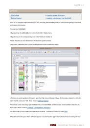
<strong>WellCAD</strong> Workspace<br />
If you start <strong>WellCAD</strong> an empty <strong>WellCAD</strong> workspace will appear on your screen.<br />
The workspace is equipped with a Frame control menu, Title bar, Tool bar, Status<br />
bar, Minimize and Maximize buttons and Restore button for the workspace window.<br />
The information contained within the Title bar, Menu bar, and Status bar will vary<br />
according to the type of active document. The Tool bar will remain the same,<br />
however, certain functions may or may not be enabled according to the active<br />
document type.<br />
Close button<br />
Restore button<br />
Minimize button<br />
Tool Bar and Title Bar<br />
The Tool bar provides quick access to the more common commands using the<br />
mouse. Some of the icons are enabled only if the context is right, e.g. Print is not<br />
accessible if the active document is not in presentation mode. The Tool bar is<br />
composed of separate components, which can be added or removed from the Tool<br />
bar individually.
BOOK 1 - WELLCAD BASICS - 3<br />
The Title bar displays the name of the program (<strong>WellCAD</strong>) and the name of the<br />
active document window.<br />
Displaying or hiding the Title bar<br />
From the View menu check or uncheck the option Title Bar.<br />
Enabling or disabling components of the Tool bar<br />
From the View > Toolbars menu, check or uncheck the desired Tool bar<br />
component. You could also use one of the available shortcuts.<br />
1.2 Borehole Documents<br />
The borehole document is the general worksheet to generate log charts. It stores and<br />
graphically displays the imported or interactively added data. File I/O operations,<br />
graphical editing and printing is carried out on documents. A header and trailer<br />
section can extend each document.<br />
<strong>WellCAD</strong> supports MS Windows multi document interface (MDI), which means<br />
that you can have more than one document open at the same time. Each document<br />
will open in its own window and will be listed in the Window menu.<br />
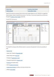
Document window<br />
Control Menu<br />
Borehole Document<br />
Title Bar<br />
Borehole Document Title<br />
Zone<br />
Borehole Document Data<br />
Area<br />
When a document is active, commands that you choose from the Menu bar or the<br />
Tool bar affect the document or the information and items contained in it. The<br />
borehole document is saved in its own file carrying the file name extension *.WCL.<br />
Borehole Document within <strong>WellCAD</strong> workspace
4 - BOOK 1 - WELLCAD BASICS<br />
www.alt.lu<br />
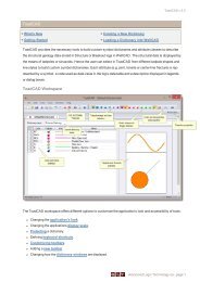
Header Element 1<br />
Header Element 2<br />
Data and TitleZone<br />
Trailer Element 1<br />
Trailer Element 2<br />
This example shows the different elements a Borehole Document is made of (Header, Titles, Data, Footer)<br />
1.2.1 Loading and Saving Borehole Documents<br />
Saving a WCL file:<br />
Borehole documents are saved as *.WCL files using the Save (CTRL + S) and<br />
Save As… options from the File menu. All down hole data hosted by the borehole<br />
document as well as the chart layout information will be saved in the *.WCL file.<br />
You can also select the Close (CTRL + F4) option from the File menu and you<br />
will be prompted to save the borehole document before the document closes.<br />
Saving a WCL in a previous file format:<br />
Borehole Document<br />
Depending on the version number of <strong>WellCAD</strong> WCL files are saved in a special<br />
format. In general <strong>WellCAD</strong> is backward compatible, which means an older file<br />
format can always be opened with a newer version of <strong>WellCAD</strong>. But if you try to<br />
load e.g. a v4.4 format with a <strong>WellCAD</strong> version 4.3, the loading will fail due to an<br />
unknown file format.
1.2.1.1 Reader Module<br />
BOOK 1 - WELLCAD BASICS - 5<br />
You can save a WCL file in the previous format by following the steps outlined<br />
hereafter. Note, that if you have used new log types or settings, which are unknown<br />
to the previous version, the file export into the previous version may fail.<br />
▪ From the File menu select Export > Single File.<br />
▪ From the file extension drop down list choose either <strong>WellCAD</strong> v4.1, v4.2 or<br />
<strong>WellCAD</strong> v4.3.<br />
▪ Click the Save button.<br />
Loading WCL files:<br />
1.2.1.2 Automation Module<br />
Borehole documents can be reloaded and displayed in the <strong>WellCAD</strong> workspace<br />
using the Open (CTRL + O) command from the File menu. The standard<br />
Windows file open dialog box will appear to let you browse for the desired *.WCL<br />
file. Alternative ways to open a borehole document file in the <strong>WellCAD</strong> workspace<br />
are to double click the file name in the Windows Explorer or simply drag the file from<br />
the Explorer into the <strong>WellCAD</strong> workspace.<br />
(You can for example load one of the sample documents contained in the Samples<br />
folder located in the installation directory of <strong>WellCAD</strong>.)<br />
The <strong>WellCAD</strong> Reader is a free data viewer for <strong>WellCAD</strong> *.WCL files. To create files<br />
that can be read by the data viewing application the Reader Module must be<br />
activated on your <strong>WellCAD</strong> license.<br />
The Automation Module allows users who have this module activated on their<br />
license to access methods and properties of various objects exposed by <strong>WellCAD</strong>.<br />
E.g. methods like FileImport, ApplyTemplate or SaveAs can be accessed in external<br />
program code. It also allows users to write Visual Basic scripts (*.VBS) to automate<br />
routine tasks in <strong>WellCAD</strong>. The Automation entry in the File menu is a convenient<br />
shortcut to run such VBS scripts on a borehole document. Due to the complexity of<br />
the Automation Syntax a separate manual has been written. Please contact ALT or<br />
visit the ALT homepage (www.alt.lu) to learn how to retrieve a copy.
6 - BOOK 1 - WELLCAD BASICS<br />
1.2.2 Creating a new Borehole Document<br />
www.alt.lu<br />
To begin with a new blank borehole document, click the New (CTRL + N)<br />
option from the File menu. The New document dialog box will appear.<br />
Document<br />
templates<br />
Current directory<br />
containing document<br />
templates<br />
New document dialog box to open a blank document<br />
Display styles for<br />
template list<br />
Document<br />
Depth Range<br />
The dialog provides a list of document types that can be created. Besides an empty,<br />
blank borehole document it is possible to load a document template of a previously<br />
created log chart. Document templates provide already a complete chart layout that<br />
can be populated with data. Templates will be explained in detail in 1.4.4<br />
Templates.<br />
Select the Blank borehole document option from the list and click OK to open a<br />
blank borehole document in the <strong>WellCAD</strong> workspace. The next step would be to<br />
load data into the document and arrange its layout.<br />
<strong>WellCAD</strong> Borehole documents are created automatically if you import data from a<br />
file (e.g. *.CSV, *.LAS or *.LIS). Data import, export and log chart formatting are<br />
explained in 1.3.2 Basic Log Editing.
1.2.3 Draft, Presentation and Print Preview Modes<br />
1.2.3.1 Presentation Mode<br />
1.2.3.2 Draft Mode<br />
BOOK 1 - WELLCAD BASICS - 7<br />
If an existing borehole document has been opened in the <strong>WellCAD</strong> workspace, it<br />
can be displayed in three different modes: Presentation, Draft and Print Preview.<br />
In presentation mode the <strong>WellCAD</strong> borehole document window displays the log<br />
chart in a WYSIWYG (What You See Is What You Get) mode. The document is<br />
displayed with header, trailer, title and data section with width, height and all scales<br />
very close to the printed result. Modifications with respect to header and title display<br />
can be made using the Header and Titles options in the View menu.<br />
Presentation mode is the preferred mode for report presentation fine-tuning.<br />
Please note that on computers with Windows 7 operating system deviations from a<br />
true WYSIWYG presentation of the borehole document may be observed. In order<br />
to adjust the display scale to show the true units on screen go to Tools > Options<br />
> Display Scale.<br />
Display Scale dialog box to map screen unit to true units<br />
In order to map screen units to true units hold a ruler against the screen and drag<br />
the displayed scale (place the cursor in the displayed scale, hold down the left mouse<br />
button and move the mouse) so that both scales show the same distances. Ensure<br />
that the unit selected from the drop down list corresponds to the units or you<br />
reference (e.g. ruler).<br />
In draft mode the width of the document is scaled to fit into the workspace window.<br />
Horizontal scrolling is not possible. The document is split into two horizontal panes,<br />
separating the log title zone from the data display area. Header and trailer are not<br />
shown on screen.
8 - BOOK 1 - WELLCAD BASICS<br />
1.2.3.3 Print Preview Mode<br />
www.alt.lu<br />
Draft mode is the preferred mode for log data editing and processing.<br />
You can switch from presentation to draft mode by selecting the Draft option from<br />
the View (CTRL + D) menu or click on .<br />
In Draft mode the View menu option Auto Adjust Splitter is available. If this<br />
option is enabled the splitter bar dividing log handles from data area is automatically<br />
positioned below the bottom most handle and the upper window is adjusted in<br />
height to displays all log handles. This option can be turned off and the user can<br />
shift the splitter bar to a new position if the title area covers too much space.<br />
In print preview mode the borehole document window displays a scaled image of<br />
the document, as it will print. This non-editable mode is intended to provide a final<br />
check of the document before printing it.<br />
To print preview a document, select Print Preview from the File menu or click the<br />
. As printing (and print previewing) is not possible for a document being in draft<br />
mode an automatic conversion to presentation mode takes place prior to the print<br />
previewing.<br />
1.2.4 Document Handling<br />
Each window can be moved, resized and scrolled as known from other Microsoft<br />
Windows compatible software (e.g. WORD, EXCEL).<br />
You can also organize multiple windows within the <strong>WellCAD</strong> workspace using the<br />
following options from the Window menu:<br />
New Window to create a new instance of the active window.<br />
Close All to exit all windows.<br />
Cascade to arrange all open windows in a cascaded manner.<br />
Tile Horizontally, Tile Vertically to arrange all windows to appear resized in<br />
horizontal or vertical order.<br />
Arrange Icons to arrange minimized windows.<br />
Nevertheless we would like to outline some actions you can perform on borehole<br />
documents that you might find useful.
1.2.4.1 Switching between documents<br />
1.2.4.2 Splitting a document<br />
BOOK 1 - WELLCAD BASICS - 9<br />
An active borehole document will have a highlighted Title Bar. To switch to another<br />
document you can either:<br />
▪ Select the new window name from the list in the Window menu.<br />
▪ From the control menu choose Next or use the shortcut CTRL + F6.<br />
▪ To make a previous window active use the shortcut CTRL + SHIFT + F6.<br />
When working on large documents it is often convenient to split the window into<br />
smaller panes in order to view all relevant information on screen at the same time.<br />
Horizontal Split<br />
Vertical Split<br />
Borehole document split into different panes<br />
Each borehole document window in presentation mode contains a horizontal and<br />
vertical split box.<br />
Vertical Split<br />
Box<br />
Horizontal<br />
Split Box<br />
To split a window into panes click and drag the split box to the desired position.<br />
Alternatively you can choose Split from the Window menu and click at the split<br />
position in the document.
10 - BOOK 1 - WELLCAD BASICS<br />
1.2.4.3 Jump to a particular depth<br />
1.3 Logs<br />
www.alt.lu<br />
Single log<br />
Document combining<br />
many logs to a composite<br />
display<br />
To join split windows simply drag the vertical split box to the left or right window<br />
limit and the horizontal split box to the top or bottom window limit.<br />
It is important to understand that multiple panes within a document window merely<br />
provide alternative views (although independently scrollable) of the parent<br />
document. They are not separate independent documents.<br />
To jump to a specific depth or time within your borehole document choose the<br />
Goto Depth option from the Edit menu or press the shortcut keys CTRL + G.<br />
Enter the desired depth or date/time you want to jump to.<br />
In order to store, display and organize down hole data of different formats in a user<br />
friendly and at all times accessible way, <strong>WellCAD</strong> deals with data containers of<br />
distinct formats – so called Logs. Logs are the key elements of a borehole document.<br />
A borehole document with a single Log (data container) on the left and populated with logs of different types on<br />
the right.<br />
Logs are created automatically when data is imported from files. The type of log is<br />
chosen according to the information provided by the imported file or the user will<br />
be asked to select a log type. Logs can also be created from scratch:<br />
� Open the Edit > Insert New Log menu<br />
� Select the log type you want to create from the list provided
BOOK 1 - WELLCAD BASICS - 11<br />
Usually the Main Settings dialog box of the new log is displayed next<br />
To see the numerical data contained in a log the Tabular Editor providing a<br />
spreadsheet of the actual data set can be called up. Additionally the user can also<br />
observe the data values of a selected log in the Status Bar of the borehole window<br />
while moving the mouse over the data set.<br />
1.3.1 Log Types and Their Characteristics<br />
An overview of all log types contained in <strong>WellCAD</strong>, their main purpose, data format<br />
and display styles, is given hereafter. A more extensive description of log types<br />
including their display settings is given in Appendix A.<br />
The following list provides for each log type:<br />
- A short description of the log’s characteristics and purpose of use.<br />
- The format of the data container. This format corresponds also to the ASCII<br />
file import /export format.<br />
- An overview of the main data presentation styles of the log.<br />
1.3.1.1 Well / Formula Log<br />
Description:<br />
Single point data sampled at a constant rate. The Well Log is used to display any<br />
kind of equally sampled geophysical data as curve (e.g. Gamma Ray, Density,<br />
Resistivity, Porosity, Transit Time). Well Log data is generally imported from LAS,<br />
LIS, DLIS or ASCII files (*.txt, *.csv) but can also be generated interactively (e.g.<br />
grain size curve in core description). Formula Logs are calculated curves using one<br />
or more Well Logs as data source. They are dynamically linked to Well Logs.<br />
Data Format:<br />
Depth, Data<br />
E.g.
12 - BOOK 1 - WELLCAD BASICS<br />
1.3.1.2 Mud Log<br />
www.alt.lu<br />
Display Styles:<br />
Description:<br />
Well Log data is always displayed as single curve<br />
Single point data sampled at a non-constant rate. The Mud Log data type handles<br />
any depth to value based data. Imported from LAS, LIS, DLIS or ASCII files (*.txt,<br />
*.csv) or generated interactively, they are used to display data such as DST data, bit<br />
penetration rates or core recovery data.<br />
Data Format:<br />
Depth, Data<br />
E.g.
Display Styles:<br />
1.3.1.3 Depth Column Log<br />
BOOK 1 - WELLCAD BASICS - 13<br />
Mud Log data can be displayed as bar, line, symbol or a combination of the former styles with the value<br />
displayed as string.<br />
Description:<br />
The Depth Column Log deals with single point data at a non-constant sample rate.<br />
Its data is displayed as a depth axis. The log can be used to handle different depth<br />
systems (e.g. MD, TVD) but allows generation of elevation or date/time axis, too.<br />
Data is generally imported from files or entered by the user. The <strong>WellCAD</strong> Depth<br />
Matcher and Deviation Process tools are able to generate a Depth Column Log.<br />
Data Format:<br />
Depth, Data<br />
E.g.
14 - BOOK 1 - WELLCAD BASICS<br />
1.3.1.4 Interval Log<br />
www.alt.lu<br />
Display Styles:<br />
Description:<br />
Depth Column Log data presented as: Depth axis, date/time axis<br />
The Interval Log handles single value per depth range data. It is possible that<br />
consecutive intervals overlap each other. Data can be imported from ASCII files<br />
(*.txt, *.csv) or generated interactively. It is, besides others, used to display blocked<br />
curve or pumping test data.<br />
Data Format:<br />
TopDepth, BottomDepth, Data<br />
E.g.
1.3.1.5 Marker Log<br />
Display Styles:<br />
Description:<br />
BOOK 1 - WELLCAD BASICS - 15<br />
Interval Log data presented as: Bar, Segment, Bar Edge Line and Classified Bar<br />
The Marker Log handles single point data. It can be used to store and display<br />
markers such as formation tops, major/minor contacts, unconformities, etc.. Its<br />
main purpose is to allow an auto correlation and automatic insertion of surfaces in<br />
the multi well module.<br />
Data can be imported from ASCII files or is manually entered by the user.<br />
Data Format:<br />
Depth, Name, Comment, Contact<br />
E.g.
16 - BOOK 1 - WELLCAD BASICS<br />
1.3.1.6 Comment Log<br />
www.alt.lu<br />
Display Styles:<br />
Description:<br />
Marker Log displaying data in Top, Surface and Marker style<br />
The Comment Log handles text in boxes, where a top and bottom depth defines the<br />
upper and lower limit of each box. Comment Logs are used to handle any kind of<br />
descriptive text within a borehole document (e.g. lithology descriptions).<br />
Data can be imported from ASCII files or is manually entered by the user.<br />
Data Format:<br />
TopDepth, BottomDepth, Text<br />
E.g.
1.3.1.7 CoreDesc Log<br />
Display Styles:<br />
Description:<br />
BOOK 1 - WELLCAD BASICS - 17<br />
Comment Log data can be presented in different font styles ant orientations<br />
The Core Description Log deals with interval data and is used to present the<br />
occurrence of a certain event over a depth range. The type of event (e.g. fossil type<br />
or drilling bit used) appears as graphical symbol that is loaded from a predefined but<br />
customizable library. In addition abundance and dominance of the feature shown<br />
can be stored and displayed.<br />
Data is generally imported from ASCII files or can be entered by the user.<br />
Data Format:<br />
TopDepth, BottomDepth, Symbol Code, Abundance,<br />
Dominance<br />
E.g.
18 - BOOK 1 - WELLCAD BASICS<br />
1.3.1.8 Lithology Log<br />
www.alt.lu<br />
Display Styles:<br />
A Core Description Log where the symbol indicates the type of feature, the line style reflects abundance and<br />
dominance is shown in the arrow tip.<br />
Description:<br />
Lithology Logs have been designed to display information about lithology,<br />
sedimentary structure etc. as box filling graphical patterns loaded from user created<br />
libraries (see LithCAD). Top and bottom contact styles can be assigned to each<br />
lithology box. The same log type can be used to display non repeated (not box<br />
filling) symbols in order to indicate lithology accessories, qualifiers etc..<br />
Often two or more lithology logs are superimposed to allow a complex lithology in a<br />
single track.<br />
Data Format:<br />
TopDepth, BottomDepth, Code, Hardness, TopContact,<br />
BottomContact<br />
E.g.
1.3.1.9 Strata Log<br />
Display Styles:<br />
BOOK 1 - WELLCAD BASICS - 19<br />
Lithology Log with box filling repeated graphical pattern (left) and non-repeated symbol ( right).<br />
Description:<br />
The Strata (Stratigraphy) Log has been developed to handle and display chrono- or<br />
litho-stratigraphy columns (e.g. System, Series and Stage) in a single log column.<br />
Manually entered text or text and color/pattern fill loaded from libraries can be<br />
displayed in boxes limited by column width and Top and Bottom Depth. Any<br />
number of columns can be handled. If text found in adjacent boxes is equal it will be<br />
merged and displayed as single box.<br />
Top and Bottom Contact styles can be assigned to each box. In order to highlight<br />
important zones (e.g. a reservoir) the user can allow contact style lines to be drawn<br />
across the entire borehole document.<br />
Data Format:<br />
TopDepth, BottomDepth, DataCol1, DataCol2,…,DataColN,<br />
TopContact, BottomContact<br />
E.g.
20 - BOOK 1 - WELLCAD BASICS<br />
www.alt.lu<br />
Display Styles:<br />
1.3.1.10 Stacking Pattern Log<br />
Strata Log with three columns. Data displayed as plain text (left) and text / color fill combined (right).<br />
Description:<br />
The Stacking Pattern log can be used to display trends within certain depth intervals<br />
such as coarsening or fining in grain size. Data values are represented by the means<br />
of geometrical figures (triangle and square). Besides Top and Bottom Depth the data<br />
format requires a normalized value (0 to 1) describing the width of the symbol at top<br />
and bottom of the interval.
Data Format:<br />
BOOK 1 - WELLCAD BASICS - 21<br />
TopDepth, BottomDepth, TopWidth, BottomWidth<br />
E.g.<br />
Display Styles:<br />
Two Stacking Pattern Logs showing different cycles of coarsening and fining (triangles) with areas of stagnation<br />
(squares). The right log highlights the box boundaries to allow correlation with lithology log intervals.
22 - BOOK 1 - WELLCAD BASICS<br />
1.3.1.11 OLE Log<br />
www.alt.lu<br />
Description:<br />
OLE is the acronym for Object Linking and Embedding. OLE is an application<br />
integration technology that can be used to share information between OLE<br />
compatible applications. In <strong>WellCAD</strong>, embedded and linked OLE objects (such as<br />
photographs, EXCEL charts, WORD documents) are handled by the OLE Log.<br />
The data consists of individual OLE objects each with a top and bottom depth.<br />
Since <strong>WellCAD</strong> version 4.2 the OLE Log can also be used to display pictures (e.g.<br />
JPEG) as Non-OLE objects. Compared to the RGB Log the OLE Log consumes<br />
fewer resources when handling large quantities of data. A picture is not converted<br />
into RGB intensity values but is stored in its original size. The user can set the<br />
default behavior of the OLE Log in the Default Settings.<br />
Data can be inserted manually or loaded from ASCII files. E.g. to import a series of<br />
core photographs simply import an ASCII file providing top and bottom depth and<br />
the path to the picture file as OLE Log.<br />
Data Format:<br />
TopDepth, BottomDepth, OleObject<br />
E.g.<br />
Display Styles:<br />
OLE Log showing an embedded EXCEL sheet and a thin section picture.
1.3.1.12 Full Wave Sonic Log<br />
Description:<br />
BOOK 1 - WELLCAD BASICS - 23<br />
FWS Log (Full Waveform Sonic) data is a two dimensional array of floating point<br />
values. One dimension consists of depth, sampled at a constant rate, the second<br />
dimension usually consists of time in �s, sampled at a constant rate, too. Thus, for<br />
each depth increment the log holds a data trace sampled in time. The FWS log is<br />
most commonly used to store and display full waveform sonic data but can also<br />
used to display borehole radar data, slowness or T2 distribution curves. The<br />
horizontal dimension can be “misused” and must not necessarily correspond to time<br />
in �s all the time.<br />
Data Format:<br />
Depth, Data1, Data2, Data3, … ,DataN<br />
E.g.<br />
Display Styles:<br />
FWS Log data presented as Wiggle, b/w VDL and color VDL.
24 - BOOK 1 - WELLCAD BASICS<br />
1.3.1.13 VSP Log<br />
www.alt.lu<br />
Description:<br />
The VSP (Vertical Seismic Profile) Log handles a two dimensional array of floating<br />
point data. One dimension consists of depth, sampled at a constant rate, the second<br />
dimension is a series of station names (e.g. geophones). Data traces are displayed<br />
along the vertical (depth) axis. The log can be used to display synthetic seismograms<br />
or seismic profiles as well.<br />
Data Format:<br />
Depth, RX1, Rx2, Rx3, … ,RxN<br />
E.g.<br />
Display Styles:<br />
VSP Log with data presented as Wiggle, Variable Area, b/w VDL and color VDL
BOOK 1 - WELLCAD BASICS - 25<br />
1.3.1.14 Image Log / Image Log Float 2 / Image Log Float 4<br />
Description :<br />
In general the Image Log handles an array of data where one dimension consists of<br />
equally sampled depth and the second dimension of radial equally sampled data<br />
values (one data point every x degree of an arc). The Image Log stores and displays<br />
acoustic scanner data (e.g. amplitude, travel time, thickness) as well as multi finger<br />
caliper or FMI data. Three different types of Image Logs exists each of them storing<br />
the data using a different data type.<br />
The Image Log Integer stores all values as unsigned integer (two bytes), which<br />
means that all values are between 0 and 65535. This is sufficient for acoustic scanner<br />
travel time and amplitude measurements or other data where no negative or decimal<br />
numbers occur. Image Log Float 2 (two bytes) and Image Log Float 4 (four bytes)<br />
types store data as floating point values, which allows proper handling of negative<br />
and decimal numbers.<br />
Data Format:<br />
Depth, Amp1, Amp2, Amp3, … , AmpN<br />
E.g.<br />
Display Styles:<br />
The Image Log supports three different display styles. Data displayed in Color<br />
Image style is presented as false color image where each data value is mapped to a<br />
color value according to a user customizable color palette. The Shifted Curve style<br />
divides the log track into equal intervals and draws all data columns as individual<br />
curves using the left border of each interval as zero baseline. All data columns are<br />
drawn as superimposed curves if the Stacked Curve style has been set.
26 - BOOK 1 - WELLCAD BASICS<br />
1.3.1.15 RGB Log<br />
www.alt.lu<br />
Image Log displayed in Color Image (left), Shifted Curve (mid) and Stacked Curve (right) style.<br />
Description:<br />
The RGB Log is used to display bitmap data such as optical televiewer images, core<br />
photographs, video snapshots etc.. Data is stored in a two dimensional array of RGB<br />
(Red, Green, Blue) intensity triplets. One dimension consists of depth, sampled at a<br />
constant rate, and the second dimension of radial equally sampled data values (one<br />
data point every x degree of an arc). Thus, for each depth increment there is a data<br />
set associated, which represents the full (or partial) coverage of a borehole wall or<br />
core circumference.<br />
Data Format:<br />
Depth, RGB 1, RGB 2, RGB 3, … , RGB N<br />
E.g.
1.3.1.16 Analysis Log<br />
Display Styles:<br />
BOOK 1 - WELLCAD BASICS - 27<br />
The RGB Log data is displayed as bitmap according to resolution and color<br />
information provided by the data values.<br />
Description:<br />
RGB Log display of optical televiewer data<br />
Analysis logs are used to present the composition of lithology or balance between<br />
different components displaying each element according to its quantity (in percent)<br />
as graphical pattern. Data is stored in a two dimensional array, where the first<br />
dimension consist of depth, sampled at a constant rate, and the second dimension<br />
holds the series of percentage values belonging to the different elements. The user<br />
can define the number and type of elements to be handled.<br />
Graphical patterns are user definable and their storage is organized by the means of<br />
lithology dictionaries. Lithology dictionaries can be created, edited and maintained<br />
using LithCAD.<br />
Data Format:<br />
Depth, Data1, Data2, Data3, … , DataN<br />
E.g.
28 - BOOK 1 - WELLCAD BASICS<br />
www.alt.lu<br />
Display Styles:<br />
1.3.1.17 Percentage Log<br />
Description:<br />
The Analysis Log supports three different data display styles.<br />
Fixed Bar style: A bar of fixed height is drawn for each depth point.<br />
Dynamic Bar style: A bar is drawn from one to the next depth point.<br />
Line style: Data points belonging to the same element are connected and displayed<br />
as curve, where the area between the curves is filled with a graphical pattern<br />
reflecting the type of element.<br />
Analysis Log data presented as Fixed Bar, Dynamic Bar and Line.<br />
The only difference between Analysis and Percentage Log is, that the depth<br />
increments for the Percentage log do not have to be constant. This results in<br />
variable bar thickness when the Dynamic Bar display style has been chosen.<br />
Data Format:<br />
Depth, Data1, Data2, Data3, … , DataN<br />
E.g.
1.3.1.18 Structure Log<br />
Display Styles:<br />
Description:<br />
BOOK 1 - WELLCAD BASICS - 29<br />
Percentage Log data shown in Fixed Bar, Dynamic Bar and Line style<br />
The Structure log can be used to pick and store planar features like joints and<br />
fractures interactively and record depth, dip angle, azimuth (dip direction), aperture<br />
and structure classes. You can also import the data from ASCII files. Please note<br />
that the data format differs from earlier versions of the Structure Log.<br />
Data Format:<br />
Depth, Azimuth, Dip, Aperture, Class1, Class2, Class3…<br />
E.g.<br />
Display Styles:<br />
The data stored in the Structure Log can be displayed in<br />
Projection Style: The great circle produced by the intersection of dipping plane and<br />
borehole is “unrolled” and appears as sinus curve.
30 - BOOK 1 - WELLCAD BASICS<br />
www.alt.lu<br />
W<br />
S<br />
N<br />
E<br />
N E S W N<br />
Unrolled great circle appears as sinus curve.<br />
Tadpole Style: Data is displayed as tadpole style arrow plot. The body of the<br />
tadpole with respect to the horizontal log scale shows the amount of dip, while the<br />
tadpole vector line indicates the azimuth (dip direction). Different tadpole colors<br />
and shapes are used to differentiate structure classes.<br />
Slab Core Projection Style: The intersection line between the dipping plane and a<br />
virtual vertical plane of distinct orientation (e.g. North to South) is displayed.<br />
Structure Log in Projection, Tadpole and Slab Core Projection style.
1.3.1.19 Breakout Log<br />
Description:<br />
BOOK 1 - WELLCAD BASICS - 31<br />
The Breakout log can be used to pick vertical features such as borehole wall<br />
breakouts and tensile fractures interactively from an image. The recorded data is<br />
depth (determined from the center of the picked feature), azimuth (position on the<br />
borehole wall in deg), tilt (inclination of the breakout axis from the borehole axis),<br />
length, opening angle in degree and one or multiple attributes. You can also import<br />
the data from ASCII files.<br />
Data Format:<br />
Depth, Azimuth, Tilt, Length, Opening, Class1, Class2,<br />
Class3…<br />
E.g.<br />
Display Styles:<br />
The data stored in the Breakout Log can be displayed as<br />
Projection Style: A line tracing or polygon framing the breakout as in the oriented<br />
and unrolled image of the borehole wall. The horizontal scale is from 0 to 360 deg.<br />
Symbol Style: The picked breakout is displayed as tadpole. The body of the tadpole<br />
with respect to the horizontal log scale shows the azimuth position. If the tadpole<br />
has been created with a vector line (in ToadCAD) it will indicate the tilt component.<br />
It is optional to display the opening angle as a horizontal bar. Different tadpole<br />
colors and shapes can be used to differentiate between breakout classes.<br />
Breakout Log in Projection and Symbol style.
32 - BOOK 1 - WELLCAD BASICS<br />
1.3.1.20 Bio Log<br />
www.alt.lu<br />
Description:<br />
Biostratigraphic Logs (short: Bio Logs) are used to display count rates of distinct<br />
features (e.g. fossils) per depth interval. The log stores and displays the count rate<br />
(floating point number) of a user-defined number of different features for each<br />
depth interval.<br />
Data Format:<br />
TopDepth, BottomDepth, Nature, Val1, Val2, … ,ValN<br />
E.g.<br />
Display Styles:<br />
Bio Log: Count rates presented in vertical and horizontal bar style (left and mid). To show only the occurrence<br />
of a certain feature a (user defined) symbol can be drawn (right).
1.3.1.21 Engineering Log<br />
Description:<br />
BOOK 1 - WELLCAD BASICS - 33<br />
The Engineering Log can be used to show construction and completion details of a<br />
well. Logs can be presented side by side to depict a diary of construction or drilling<br />
events. Objects such as different casing, cementation, gravel pack, water and more<br />
can be combined and displayed.<br />
Four different kinds of symbol classes are supported:<br />
- Drill Items, they are characterized by a top depth, bottom depth and an external<br />
diameter. They present the drill hole itself.<br />
- Solid Items, these are cylindrical items which occupy a volume in the borehole<br />
(such as a packer). A top depth, bottom depth, an external diameter and a radial<br />
position within the hole describe them.<br />
- Hollow Items are cylindrical and occupy a volume in the borehole with an<br />
internal space that can be filled with any other liquid or solid item. A typical<br />
example is a casing. A top and bottom depth, an external diameter, an internal<br />
diameter and a radial position in the hole characterize hollow items.<br />
- Liquid Items fill all accessible borehole volume within a given depth range from<br />
a given injection point (e.g. cement or water). A top depth, bottom depth,<br />
injection point and radial position describe liquid items.<br />
Data Format:<br />
Item, TopDepth, BottomDepth, Position, External<br />
Diameter, Internal Diameter, Injection Depth<br />
E.g.
34 - BOOK 1 - WELLCAD BASICS<br />
1.3.1.22 Shading Log<br />
www.alt.lu<br />
Display Styles:<br />
Engineering Log with drill item (borehole), hollow item (casing) and liquid items (cement, water).<br />
Description:<br />
The Shading Log is no real log type, as it contains no own data. Shading logs use<br />
one or two Well Logs to fill the area between two curves, curve and log border or<br />
curve and user defined limit with a solid color.<br />
Display Styles:<br />
Shading Log used to fill the area between two curves (left), between track border and curve (mid) and between<br />
fixed limit and curve (right).
1.3.1.23 Polar & Rose Log<br />
Description:<br />
BOOK 1 - WELLCAD BASICS - 35<br />
The Polar & Rose Log is dynamically linked to a Structure or Breakout Log. Its<br />
purpose is to display a summary of the structure or breakout data from a distinct<br />
depth interval in various diagrams such as polar projection plots, dip and azimuth<br />
histograms, rose diagrams, vector plots or Woodcock diagrams. The only data stored<br />
in the Polar & Rose Log is the top and bottom of the depth interval where the<br />
structure or breakout data has been taken from and a text comment. Multiple<br />
diagrams of different depth intervals can be displayed within the same log.<br />
Data Format:<br />
TopDepth, BottomDepth, Description<br />
E.g.<br />
Display Styles:
36 - BOOK 1 - WELLCAD BASICS<br />
1.3.1.24 Cross Section Log<br />
www.alt.lu<br />
Polar & Rose Log diagrams: Polar Projection plot (left), Rose Diagram (mid left), Dip Histogram (mid<br />
right), Max Horizontal Stress direction (right, Vector plot (lower left) and Woodcock diagram (lower right)).<br />
Description:<br />
The Cross Section Log can be used to display cross sections of the borehole cylinder<br />
using caliper (or travel time) information at a certain depth or from a depth interval.<br />
The Log must be linked to an Image Log providing the caliper information. Only<br />
top and bottom depth of the cross section intervals are stored.<br />
Data Format:<br />
TopDepth, BottomDepth<br />
E.g.
1.3.1.25 3D Log<br />
Display Styles:<br />
Description:<br />
BOOK 1 - WELLCAD BASICS - 37<br />
Cross Section Log data: Superimposed measurements (left), average of measurement (right)<br />
The 3D Log displays a three dimensional image of the borehole cylinder using<br />
caliper information to model the shape of the cylinder and amplitude information to<br />
map colors to the cylinder surface. The log must be linked to Image or Well Logs in<br />
order to retrieve the caliper and amplitude data. The 3D Log itself does not store<br />
any data.<br />
Display Styles:<br />
3D Log display as fully rendered cylinder (left) or as wire frame (right)
38 - BOOK 1 - WELLCAD BASICS<br />
1.3.2 Basic Log Editing<br />
www.alt.lu<br />
The following paragraphs will describe some fundamental operations that can be<br />
carried out on logs. Knowledge about how to select, position or rename a log is<br />
essential for working with <strong>WellCAD</strong>. More specific information on how to create a<br />
lithology column, filter and resample data can be found in 1.5 Working with Logs.<br />
Details about the functionality of <strong>WellCAD</strong> add-on modules can be found in the<br />
relevant books.<br />
All log types have a title zone – or log handle – that displays the name of the log and<br />
other properties of the log. It acts as a handle for selecting, moving, sizing or scaling<br />
the log within the borehole window.<br />
Log title<br />
(log handle)<br />
Log data area<br />
1.3.2.1 Selecting Logs in a Borehole Document<br />
Before any action can be carried out on a log or its data, the log(s) must be selected.<br />
To select a log simply click once onto its log handle. The handle color becomes<br />
inverted to indicate the selected status.<br />
Log not selected<br />
Selected log<br />
If you want to select multiple logs hold the CTRL key pressed while clicking on the<br />
log handles.<br />
To deselect a log, hold down the CTRL and click on the handle of the selected log.<br />
You can also click outside a log (without pressing the CTRL key), but this will<br />
deselect all multiple selected logs as well.
BOOK 1 - WELLCAD BASICS - 39<br />
An alternative way to select or deselect logs is provided by the Tracks Selection<br />
dialog box.<br />
Selected log names from the list<br />
To call up this dialog box click the icon or choose the Select option from the<br />
Edit > Select Tracks menu. Click on the log names in the list to select the<br />
corresponding logs. Hold the CTRL or SHIFT keys down to allow multiple<br />
selections.<br />
Note:<br />
If you select multiple logs you might have noticed that the first log selected gets a<br />
red frame around its handle. This becomes important if document layout tools are<br />
used to arrange the logs within the borehole document. The first log selected will be<br />
used as a reference to adjust track width, title height and position of all other<br />
selected logs.<br />
Selecting hidden log titles:<br />
Sometimes log titles are hidden by the user. In order to display these hidden log<br />
titles select View > Show all titles or press the key combination<br />
CTRL + SHIFT + A.<br />
1.3.2.2 Creating and Deleting Logs<br />
Logs can be created in various ways. They will be created automatically for you if<br />
data is imported from a file. The log type created will be chosen either automatically<br />
according to the type of data imported or the user can select the type of log himself,<br />
as it is for the import of ASCII data.<br />
But the user can create empty logs directly in the borehole document and populate<br />
them with data (e.g. lithology patterns or descriptive text) afterwards. To create a<br />
new empty log:
40 - BOOK 1 - WELLCAD BASICS<br />
www.alt.lu<br />
� Insert a new borehole document or load an existing one.<br />
� Select Insert New Log … from the Edit menu.<br />
� Select the log type from the list.<br />
Select the type of log to<br />
be inserted from the<br />
menu.<br />
Depending on your selection it will be either the Main Settings dialog box that<br />
pops up requesting information such as log title, log position and presentation styles,<br />
or it will be another dialog boxes prompting for logs to be specified that will be used<br />
as data source (e.g. you can create a new Image Log from multiple Well Logs).<br />
Details for each log type can be found in Appendix A.<br />
To delete an existing log:<br />
� Select the log(s) you want to delete.<br />
� Press the DELETE key on your keyboard, select Edit > Delete from the<br />
menu or click the icon.<br />
Another way to delete a log is to<br />
� Right click onto the log handle and select Delete from the appearing flying<br />
menu.
1.3.2.3 Naming Logs<br />
Right click on log handle and<br />
select delete to destroy the log<br />
BOOK 1 - WELLCAD BASICS - 41<br />
If you just want to erase the data from a log without removing it from the<br />
document:<br />
� Right click on the log title(s) from which you want to erase the data.<br />
� From the context menu that opens select the Clear Contents option.<br />
You can change the title of a log within the Main, Base and Title Settings dialog<br />
boxes. (All of these dialog boxes are explained in detail further down.)<br />
� Double click onto a log handle to call up the Main Settings dialog box for that<br />
particular log.<br />
� Enter the new log name into the Title edit box.<br />
You can also select the log and click the icon (or CTRL + B) for the Base<br />
Settings or the icon for the Main Settings dialog box (or CTRL + M). Simply<br />
enter the new log name in the Title edit box.<br />
Click the icon (or CTRL + T) to display the Title Settings dialog box on<br />
screen.<br />
Select the Title part<br />
Click on Text to change<br />
the log name
42 - BOOK 1 - WELLCAD BASICS<br />
www.alt.lu<br />
� From the Display Settings list click on the Title part to select it.<br />
� Click the Text button next and enter the new log name into the appearing edit<br />
box.<br />
Note:<br />
1.3.2.4 Positioning Logs<br />
Logs can be linked to each other to act as a data server or they are used in<br />
calculations. Therefore each log title is used as a unique identifier for that<br />
particular log. You cannot have two or more logs with the same title within the same<br />
borehole document even if they differ in log type. <strong>WellCAD</strong> changes the log title<br />
automatically and adds an extension like #1 or #2 to avoid having twice the same<br />
log title. If you would like to display equal names please display the Comment and<br />
hide the Title display.<br />
Log titles can be renamed automatically during file import or when applying a<br />
template using an Alias Template. You will learn about Alias Templates in the<br />
corresponding chapter.<br />
You can force log names to be renamed using the Alias Table (see 1.4.2 Data<br />
Import). From the Edit menu select Rename Logs. An editor window will open<br />
listing all current log titles of your borehole document in the left column. Click into<br />
the corresponding cell in the New Name column to set a new title. Click the Use<br />
Aliases button to change the names according to the currently loaded (Tools ><br />
Options > Alias Table) Alias Table.<br />
Logs can be positioned anywhere on the borehole document. They may also overlap<br />
each other. You can enter a left and right position value in the Main, Base and<br />
Title Settings dialog box or you can use your mouse pointer to interactively change<br />
the position and width of a log.<br />
You can switch on a snap option to allow a more convenient positioning of logs. In<br />
combination with the short cuts from the Layout Toolbar you should be able to<br />
arrange logs very fast.<br />
Snap<br />
To enable the snap option:<br />
� Select Ruler bar settings… from the View menu.<br />
Or<br />
� Ensure the Ruler Bar is displayed at the top of your borehole window.<br />
� If not: Select the Ruler Bar option from the View menu.
Tick to enable snap to<br />
specified multiple of the<br />
unit<br />
Select the unit you want<br />
the horizontal position<br />
to be measured in<br />
BOOK 1 - WELLCAD BASICS - 43<br />
� Double click the Ruler Bar or Right click on it and select Settings.<br />
The Ruler bar settings dialog box opens. Select the units you want to measure your<br />
horizontal position in and tick the Enable snap option. Enter a number into the<br />
Column Position Snap edit box to set the snap step.<br />
Sizing Logs<br />
If you move the mouse pointer close to the left or right edge of a log handle the<br />
pointer changes its shape to a cross with arrow tips on the horizontal arms .<br />
� Now click and drag the side of the log to its new position.<br />
If the cursor changes to a cross<br />
with arrow tips, click and drag<br />
the edge of the log to its new<br />
position<br />
Note:<br />
You can also use the Layout Toolbar to easily make multiple logs the same size.
44 - BOOK 1 - WELLCAD BASICS<br />
www.alt.lu<br />
Moving logs<br />
When moving the mouse pointer into the center of the log handle of a log the<br />
cursor changes to a bold black arrow .<br />
� Now click and drag the entire log track to any position on the borehole<br />
document. The width of the log track will be maintained.<br />
If the cursor changes to an arrow<br />
shape, click and drag the log to its<br />
new position<br />
If you want to move multiple logs at the same time, select them and hold down the<br />
Shift key. Click into the center of one of the log handles and drag it to the desired<br />
position. When releasing the mouse button all selected logs will move to align left<br />
with the dragged log and they will adjust their width to match the one of the dragged<br />
log.<br />
Note:<br />
1.3.2.5 Layout Toolbar<br />
The Document Layout Bar<br />
provides short cuts to most<br />
commonly used layout operations<br />
You can also use the Layout Toolbar to easily move and align logs relative to each<br />
other.<br />
The Document Layout Bar provides a selection of tools, which allow the user to<br />
easily move and size logs relative to a reference log. Operations such as Make Same<br />
Width, Align Side By Side or Insert After will be mostly used when arranging log<br />
within the borehole document.<br />
You can select all document layout options from the View > Document Layout<br />
menu, but all tools are also assembled in a tool bar, which allows much faster access.
To display the Document Layout Bar:<br />
BOOK 1 - WELLCAD BASICS - 45<br />
� Select View > Toolbars > Document Layout Bar or press the short-cut<br />
CTRL + 7.<br />
You may have noticed that if logs are selected the first log chosen is surrounded by a<br />
red frame. The red-framed log handle is used as reference (or master log) for all the<br />
operations explained below. E.g. if multiple logs are selected and you click on Make<br />
Same Width all logs will be become of the same width as the master log.<br />
Making same width / height<br />
Select all the logs for which you want the title box to become the same width /<br />
height as the reference log. Ensure that the log you want to use as reference has<br />
been selected first and is surrounded by a red frame.<br />
Click on the icon to make the log title boxes the same width.<br />
Before making logs the<br />
same width<br />
After making logs the<br />
same width<br />
Before making log titles the<br />
same height<br />
Click on the icon to make all log title boxes the same height.
46 - BOOK 1 - WELLCAD BASICS<br />
www.alt.lu<br />
After making log titles the<br />
same height<br />
Before aligning logs left / right<br />
After aligning logs left<br />
After aligning logs right<br />
Align left / right / side-by-side<br />
To align a selection of logs with the left or right border of the reference log click the<br />
icon to align them left or the icon to align them right. Or click to<br />
superimpose the selected log(s) to the master log.<br />
If you want to align the selection of logs side-by-side, click on to align all logs<br />
right of the master log. The logs will be lined up in the order they were selected.<br />
Before aligning logs<br />
side-by-side
After aligning logs<br />
side-by-side<br />
Insert before / after<br />
BOOK 1 - WELLCAD BASICS - 47<br />
Select your logs and click the icon to insert the selection left of (in front of) the<br />
reference log. Click the icon to insert the selection right of (behind) the master<br />
log. The document width will be increased automatically if there is insufficient space<br />
to place the logs.<br />
Auto Fit<br />
Before Auto Fit<br />
Click the icon to remove all gaps between logs and adjust the document width so<br />
that the right border is lined up with the right most log border. This process is<br />
independent from the selection of logs.<br />
After Auto Fit: gaps are<br />
removed and document width<br />
has been decreased<br />
If you do not want to decrease the document width you can select the Move Left<br />
option from the View > Document Layout menu. (This option has no icon in the<br />
tool bar.)<br />
Stretch<br />
If you want to remove all gaps between logs and stretch all logs so that they fit into<br />
the document you have to select the Stretch option from the View > Document<br />
Layout menu. All logs will be resized relative to their original with.
48 - BOOK 1 - WELLCAD BASICS<br />
www.alt.lu<br />
Before applying Stretch<br />
After applying Stretch (independent of<br />
log selection)<br />
After applying Stretch Selection (stretch<br />
only between Master and Log 2)<br />
If you want to stretch logs to fit into the limits given by the most left and most right<br />
log border found in a selection of logs, you can use the Stretch Selection option<br />
from the View > Document Layout menu.<br />
Move up / down<br />
You can alter the vertical order of the logs by using the move up or down icons<br />
. Please note that this option is available only for a single log selected and if logs<br />
are stacked.<br />
Note:<br />
Before (left) and after (right) moving the selected log up<br />
The order of superimposed logs can be important as it defines the order of painting.<br />
The first log painted is the one at the top. If you want to cover parts of a Lithology
BOOK 1 - WELLCAD BASICS - 49<br />
Log with an opaque color of a curve shading (Well Log), you should ensure that the<br />
log handle of the Lithology Log is on top of the log handle of the Well Log.<br />
Grouping Logs<br />
The Grain Size log has been moved down (right)<br />
in order to allow the white shading to cover the lithology.<br />
Multiple logs can be combined to form a group. A group title (handle) allows<br />
handling the group like a single log in terms of positioning and resizing.<br />
A group formed by multiple logs
50 - BOOK 1 - WELLCAD BASICS<br />
1.3.2.6 Slicing and Merging Logs<br />
www.alt.lu<br />
To build a group:<br />
� Select the logs you would like to group.<br />
� Click the icon in the Layout Bar and select the Group option from the<br />
�<br />
drop down list.<br />
The group title settings dialog box appears which allows setting a title and a<br />
comment similar to the log title.<br />
Once a group has been build you can arrange the logs within the group as usual. To<br />
add a log to an existing group:<br />
� Select the group and afterwards the log you want to add.<br />
� Click the icon in the Layout Bar and select the Add To Group option<br />
from the drop down list.<br />
The group control in the Layout Bar can also be used to remove a selected log from<br />
a group or to destroy the group (ungroup).<br />
If you want to copy the title settings from one log to another you can use the Copy<br />
Title Settings option from the Edit menu. Select the source log first and the target<br />
log(s) afterwards.<br />
Logs can be sliced, which means that the user can split the data set at a certain depth<br />
and generate new logs for each resulting subset. On the other hand the other can<br />
merge logs, which means multiple data sets can be joined to form a single log.<br />
To merge an existing log:<br />
� Select the logs you want to slice.<br />
� Right click on the log handle and from the popup menu select the Slice at …<br />
option.<br />
Or<br />
� From the Edit menu choose Slice logs at… .<br />
Enter depth at which<br />
the data set will be split
1.3.2.7 Depth Shifting Logs<br />
BOOK 1 - WELLCAD BASICS - 51<br />
The Logs Slice At dialog pops up. Enter the depth at which you want to split the<br />
data set.<br />
Specify what should be<br />
created<br />
Next the Log Slice Options dialog comes up asking whether to keep the original<br />
log or to delete it after the subsets have been created. The user can decide to<br />
generate a log containing the upper part of the split data set and/or generate a log<br />
for the lower subset of the data.<br />
Top and Bottom log<br />
generated after slicing<br />
Log 1<br />
In order to apply a constant shift in depth to one or more logs:<br />
� Select the logs you want to shift.<br />
� Right click on a log handle and select Shift by… from the popup menu.<br />
Or<br />
� Select Shift logs by… from the Edit menu.
52 - BOOK 1 - WELLCAD BASICS<br />
www.alt.lu<br />
Enter depth span to<br />
entire data set shift up<br />
or down<br />
1.3.2.8 Merging Equal Items<br />
Enter the depth span by which you want to shift the data set. As depth is counted<br />
positive when going downwards, you will have to enter a positive value to shift your<br />
data set down, a negative number to shift the data upwards.<br />
A copy of the original log (data set) will be generated and added to the borehole<br />
document containing the shifted data.<br />
A constant depth shift has been<br />
applied and a shifted copy of the<br />
original log has been inserted<br />
Note:<br />
This process applies a constant shift only. In order to depth match a data set against<br />
a given reference – and apply non-linear shifts – you have to use the Depth<br />
Matcher tool (1.7.1 Depth Matching).<br />
If log types dealing with interval data – Litho, Comment, CoreDesc and Interval<br />
Logs – are used, data values of adjacent intervals might be equal. To merge all<br />
intervals with equal data together, choose the Merge Log Items command from<br />
the Edit menu.
1.3.2.9 Extending Logs<br />
1.3.2.10 Cut, Copy and Paste Logs<br />
BOOK 1 - WELLCAD BASICS - 53<br />
Equal lithology data(left) has been merged (right)<br />
Well and Analysis Logs store data only for a defined depth range. In order to add<br />
data points the user has to extend the depth range.<br />
� Right click on the log handle and select Extend from the popup menu.<br />
� Enter the new top and/or bottom depth value to extend the log to the top<br />
and/or bottom.<br />
The new depth intervals will be populated with No Data (NULL) values and depth<br />
information according to the depth sample rate of the log.<br />
Logs can be copied (or cut) from one borehole document and pasted into another<br />
document. The target document can be a <strong>WellCAD</strong> borehole document or a<br />
document from another application such as EXCEL or Word.<br />
When you copy data, <strong>WellCAD</strong> duplicates the information and places a copy onto<br />
the Windows Clipboard. When data is cut, <strong>WellCAD</strong> removes the original data from<br />
the active document and places it onto the clipboard.<br />
To copy or cut logs:<br />
� Select the logs you want to copy.<br />
� From the menu bar choose Edit > Copy (Edit > Cut) or right click on a log<br />
handle and from the popup menu select Copy (Cut). You could also press the<br />
key combination CTRL + C (CTRL + X) or click the<br />
To paste logs:<br />
icon ( ).<br />
� Activate the document you want to paste the data to.<br />
� If it is a <strong>WellCAD</strong> document you can select Edit > Paste or use the short cut<br />
CTRL + V. You can also click the icon.
54 - BOOK 1 - WELLCAD BASICS<br />
www.alt.lu<br />
For other than <strong>WellCAD</strong> documents the process to paste log data might vary.<br />
You can also copy data from other applications into <strong>WellCAD</strong> using the Windows<br />
Clipboard. E.g. Select a Depth and a Data column in EXCEL. In EXCEL choose<br />
Edit > Copy. In <strong>WellCAD</strong> go to Edit>Paste Special and select the Text option.<br />
Select Paste…<br />
... as Text<br />
Your data will be copied from EXCEL into the Windows Clipboard, which will be<br />
used as buffer.<br />
The Text File Import Wizard will pop up and guide you through the import<br />
options (see 1.4.2.2 TXT, CSV and ASCII Import).<br />
Drag’n Drop Data between <strong>WellCAD</strong> Documents:<br />
Single or multiple selected logs can be copied or cut and pasted between borehole<br />
documents by drag and drop. Conceptually drag and drop is like using the clipboard<br />
with cut or copy and paste, but it leaves the clipboard unchanged and is a more<br />
efficient way of moving data between documents.<br />
To cut and paste a single log from one document to another using drag and drop:<br />
� Ensure that the two documents are visible.<br />
� Click on the log Handle and continue holding down the mouse button.<br />
� Drag the log from one borehole window into the other. Releasing the<br />
mouse button completes the move.<br />
To copy and paste a single log from one document to another using drag and drop:<br />
� Ensure the two documents are visible.<br />
� Click on the log Handle and continue holding down the mouse button.
BOOK 1 - WELLCAD BASICS - 55<br />
� Press the CTRL key and drag the log from one borehole window to the<br />
other. Releasing the mouse button completes the move.<br />
Similarly multiple logs can be dragged and dropped if multiple logs are selected.<br />
Note that the SHIFT and CTRL keys have a different meaning while performing a<br />
log selection or a drag-drop operation:<br />
� While performing a log selection, i.e. Click on a log Handle:<br />
Simple click selects the log, eventually deselecting all previously selected<br />
logs.<br />
CTRL + Click toggles the log selection, leaving the rest of the selection<br />
unchanged.<br />
SHIFT + Click leaves the selection unchanged.<br />
� While performing a drop operation, i.e. releasing the mouse button over a<br />
possible drop area:<br />
Simple Drop or SHIFT + Drop moves the selected logs to the drop area.<br />
CTRL + Drop copies the selected logs to the drop area.<br />
The Clipboard<br />
The clipboard is a Microsoft Windows built in feature that applications use to<br />
exchange data. It can be perceived as a shared buffer. <strong>WellCAD</strong> is capable of<br />
copying four different families of Borehole Document information to the clipboard.<br />
<strong>WellCAD</strong> Borehole Logs Native Binary Format<br />
Although this format completely describes the data and the way it is presented in<br />
<strong>WellCAD</strong>, it can only be read and written by <strong>WellCAD</strong> itself. It is the preferred<br />
format used to copy and paste data within <strong>WellCAD</strong>, e.g. from one borehole<br />
document to another, or within the same document. This format is used to copy a<br />
selection of single or multiple logs.<br />
Graphical Formats<br />
<strong>WellCAD</strong> can copy a bitmap or a metafile to the clipboard. It is graphical copy of<br />
the Borehole Document as is appears on the screen. This allows you to paste an<br />
image to a graphical application such as Paintbrush, Word, Microsoft Publisher,<br />
Corel Draw etc. This format is used to copy documents in their entirety, i.e.<br />
containing all logs.
56 - BOOK 1 - WELLCAD BASICS<br />
www.alt.lu<br />
Text Formats<br />
<strong>WellCAD</strong> is capable of reading and writing various text based clipboard formats<br />
including TXT, CSV, WA* (see 1.4.2.2 TXT, CSV and ASCII Import). As for the<br />
text format the clipboard format is the same as the equivalent ASCII file format.<br />
This format is used to copy a selection of single or multiple logs.<br />
OLE Object Format<br />
1.3.2.11 Interactively Inserting Data<br />
1.3.2.12 Erasing all data from a log<br />
<strong>WellCAD</strong> supports the exchange of data using the OLE Data Object format. This<br />
format allows linking and embedding OLE objects into OLE enabled applications,<br />
to produce compound documents. <strong>WellCAD</strong> can export its documents as OLE<br />
objects (i.e. <strong>WellCAD</strong> is an OLE server) and import other applications OLE<br />
objects (i.e. <strong>WellCAD</strong> is an OLE container. This format is used to copy <strong>WellCAD</strong><br />
Borehole documents in their entirety or single OLE Logs containing OLE objects. ).<br />
For more details about these features, refer to 1.7.4 Embedding Borehole<br />
Documents.<br />
Most log types allow interactive insertion of data points. That means you can use<br />
your mouse in combination with your keyboard to “draw” data points directly into<br />
the data view of the borehole document. You can also enter data into a spreadsheet<br />
using the tabular editor. In any case the log you are going to edit must be selected.<br />
If and how data can be inserted depends on the log type. Details for each log type<br />
can be found in Appendix A. As a general rule of thumb you should remember the<br />
following:<br />
- Data can be edited only if a log is selected.<br />
- To insert data press the SHIFT key and use your mouse.<br />
- To delete data use your mouse while the CTRL key is pressed.<br />
You can easily delete all data from a log:<br />
� Right click on the title of the log from which you want to erase all data. You can<br />
also select multiple logs and right click on one of the selected log titles to erase<br />
data from multiple logs.<br />
� From the context menu select Clear Contents.<br />
This will remove all data from the log(s) without deleting the log(s) itself.
1.3.2.13 Comparing Log Data – The Tracking Bar<br />
BOOK 1 - WELLCAD BASICS - 57<br />
The Tracking Bar is a tool to view and compare data values of multiple logs<br />
originating from the same depth in a window floating on top of the borehole<br />
document. As the mouse cursor is moved along the borehole document the actual<br />
depth position will be determined and used to refresh the values displayed in the<br />
Tracking Bar.<br />
Tracking Bar showing values of multiple Logs at cursor depth<br />
The Tracking Bar can easily be displayed by pressing the key combination CTRL+9<br />
or selecting the Tracking Bar entry from the View > Toolbars menu. If you select<br />
the log titles before the box will already be filled with your selection.<br />
The bar is docked to the bottom of the borehole document by default. If you wish<br />
to make it floating on top of your borehole document simply drag or double click<br />
the left or right border to undock the bar. If you wish to have it docked again simply<br />
double click on the frame of the window.<br />
Adding a log:<br />
The easiest way to add logs to the Tracking Bar is having the logs selected prior to<br />
calling up the bar (i.e. select one or multiple logs and press CTRL+9).<br />
If you wish to add a log to an existing display simply click into the next free cell in<br />
the Log column in order to display a drop down list with all log titles available.<br />
To change to another log simple click in the corresponding cell in the Log column<br />
and pick a new log title.<br />
Removing one or multiple logs:<br />
To remove a single log from the list select the row and hit the Delete key.<br />
To clear the entire list right click into the list and select Remove all logs.
58 - BOOK 1 - WELLCAD BASICS<br />
1.3.2.14 The Tabular Editor<br />
www.alt.lu<br />
As already mentioned, logs are container to store and present log data according to<br />
the log type in a borehole document as curve, pattern, bar, etc.. The data stored in a<br />
log can be viewed and edited in a spreadsheet using the Tabular Editor.<br />
Tabular Editor view of Well, Interval and CoreDesc Log<br />
The format in which the Tabular Editor shows the log data corresponds to the data<br />
format of the log type. If you want to import data from an EXCEL sheet or an<br />
ASCII file, ensure you provide the data in the same format as you can see in the<br />
Tabular Editor.<br />
The Tabular Editor view is displayed in separate windows for each log and the<br />
information displayed in the tables is dynamically linked to the log. In other words,<br />
if you edit values in the Tabular Editor view the changes will immediately be<br />
reflected in the graphical display of the borehole document and vice versa. The<br />
depth information is always displayed in same units as the current depth scale of the<br />
Borehole Document.<br />
The appearance of the tabular editor can be changed in the default settings. Open<br />
the Tools > Options menu and choose Tabular Editor from the tree control.<br />
Make your selection of font style and background color for the spread sheet header<br />
and columns. You can pick different background colors for editable and not editable<br />
cells.<br />
To open a Tabular Editor:<br />
� Select the log for which you want to call up the Tabular Editor.<br />
� Click the icon, press CTRL+E or choose Tools > Tabular Editor…. You<br />
can also right click on the log handle and select Editor… from the popup menu.<br />
The Tabular Editor window can be handled as the Borehole Document window in<br />
terms of resizing, scrolling and splitting. You can use the options from the
1.3.2.15 Find and Replace data<br />
BOOK 1 - WELLCAD BASICS - 59<br />
Windows menu to easily arrange Borehole Document and Tabular Editor windows<br />
on your screen.<br />
Most of the cell values can be edited. Nevertheless there are some exceptions. For<br />
log types requiring a constant depth sampling rate you cannot edit the depth values.<br />
In case depth values are editable <strong>WellCAD</strong> automatically corrects the new<br />
information to keep an order of increasing depth.<br />
To edit values:<br />
� Click the cell you want to edit and type in the new value. If the value is based<br />
on a dictionary (e.g. lithology codes) its contents will be shown and you can<br />
pick a new value from the drop down list.<br />
� Press the Enter key or Click into another cell to confirm the change.<br />
To insert a new data row:<br />
� Click where you want to insert a new row.<br />
� From the Row menu select Insert before or Insert after to add a new data<br />
row.<br />
Or<br />
� Hold down the SHIFT key and click between two rows (or above the first row<br />
and below the last row) when the mouse pointer changes to an insert symbol.<br />
Default depth values will be provided. The options to insert a new data row are only<br />
enabled for log types, which do not require a constant depth sample rate. For these<br />
log types the allocated data range must be extended (see Basic Log Editing – Extend<br />
Logs).<br />
To delete a data row:<br />
� Click the row you want to delete.<br />
� From the Row menu select Delete to remove the entire data row.<br />
Or<br />
� Hold down the CTRL key and click the row you want to delete when the<br />
mouse pointer appears as delete symbol.<br />
To find and replace data values within a log, display the log’s data in the Tabular<br />
Editor. From the Edit menu select the Find/Replace option or press the short cut<br />
key CTRL + H. The following dialog box will open:
60 - BOOK 1 - WELLCAD BASICS<br />
1.3.2.16 Converting Logs<br />
1.3.2.17 The Undo Button<br />
www.alt.lu<br />
In the first line of the dialog enter the value you would like to replace. The second<br />
line should contain the new value. The example shown in the dialog box above<br />
replaces the lithology code 1288 by the string Sst. Use the Replace or Replace All<br />
button to alter only the current or all data values. If the Match entire cell contents option<br />
is not checked the “Find” algorithm will look for the specified part of the data value<br />
only and will only replace this part of the value. E.g. finding Sand and replacing it by<br />
S will find the value SandStone. After replacing it the new value will be Sstone.<br />
Most logs can be converted to other log types in order to use different presentation<br />
styles and data format. E.g. a Mud Log can be converted into a Well Log in order to<br />
perform calculations with the formula parser or a Lithology Log can be converted<br />
into a Comment Log to get a quick lithology description column in text format.<br />
� Select the log you want to convert.<br />
� Open the Edit > Convert Log To menu.<br />
� Click the log type you want to convert to (not possible conversions are grayed).<br />
The conversion options for each log type are explained in Appendix A.<br />
Since <strong>WellCAD</strong> version 4.2 an optional Undo functionality is supported. As the<br />
Undo functionality may slow down the workflow when dealing with large data<br />
volumes (i.e. a memory copy needs to be made for each Undo step) the Undo can<br />
be switched on or off. This can be done on the Undo tab in the Tools > Options<br />
dialog.
BOOK 1 - WELLCAD BASICS - 61<br />
Check the Enable Undo… option to activate the functionality. It is turned off by<br />
default. You can also adjust the number of undo levels and the amount of memory<br />
allocated during the recording steps. Change these settings only if your computer is<br />
equipped with enough memory (the above settings are use on a computer with 1 GB<br />
RAM).<br />
To Undo or Redo an action use the corresponding icons from the toolbar or<br />
entries in the Edit menu. The short-cut keys CTRL+ Z (Undo) and CTRL+Y<br />
(Redo) are supported as well.<br />
1.3.3 Log Settings<br />
Three different kinds of settings can be applied to a log. Settings, which are<br />
common to all log types, such as track border style, position or background color,<br />
are assembled in the Base Settings. Each log type supports different presentation<br />
styles for its data. These settings are controlled by the Main Settings. The options<br />
provided by the Main Settings dialog boxes differ from log type to log type. Title<br />
Settings are the third type of settings we can apply to a log. They are purely related<br />
to the layout and appearance of the title zone (handle) of each log.<br />
1.3.3.1 Base Settings<br />
The settings common to all log types are edited through the Log Base Settings<br />
dialog box.<br />
The Base Settings dialog box offers the same options to all log types.
62 - BOOK 1 - WELLCAD BASICS<br />
www.alt.lu<br />
There are different ways to access the Base Settings dialog box:<br />
�<br />
Or<br />
Select the log(s) and click the icon or press CTRL + B.<br />
�<br />
Or<br />
Right click on the log handle and select Settings > Base Settings… from the<br />
popup menu.<br />
� Select the log(s) and choose Log Settings > Base Settings… from the View<br />
menu.<br />
The following options can be set:<br />
Title:<br />
The edit box shows the current title (unique identifier) of the log. To alter the title,<br />
simply enter the new name of the log. Be aware that <strong>WellCAD</strong> adds an extension in<br />
case another log with the same title already exists.<br />
Set the new log name in the Title box.<br />
Position:<br />
You can set the left and right position of the log track in selected units. The default<br />
unit displayed is the one set for the Ruler Bar (see 1.3.2.4 Positioning Logs).<br />
Set the left and right limits of the log border and select the unit you want the position to be measured in.
General settings:<br />
Check to hide the depth grid<br />
display<br />
Entire data display can be hidden<br />
BOOK 1 - WELLCAD BASICS - 63<br />
Mask horizontal grid:<br />
Tick this option to avoid the depth grid lines (horizontal lines) to be drawn.<br />
Log with depth grid lines (left) and without (right)<br />
Mask contacts:<br />
Check this option if you want to hide the contact line crossing the log track.<br />
Contact crossing all tracks<br />
Selected log tracks with contact hidden<br />
Hide the display of contacts<br />
Hide the display of the log<br />
handle<br />
Data cannot be interactively<br />
edited when checked
64 - BOOK 1 - WELLCAD BASICS<br />
www.alt.lu<br />
Hide title display:<br />
If the user wants to hide only the display of the log title the Hide title display<br />
option should be checked. This option is particularly useful if multiple logs are<br />
superimposed to generate a complex presentation of the same parameter.<br />
Hidden titles (log handles) can temporarily be made visible – only visible log handles<br />
can be selected – using the Show all titles option from the View menu. You can<br />
also click on to select a track.<br />
Hide data display:<br />
A borehole document stores all data contained in the logs – even if the logs are<br />
hidden. To keep a copy of the original data set in the document without displaying<br />
the data you can hide the title and data display. To hide the data display, check the<br />
Hide data display option.<br />
Lock log data:<br />
Most log types in <strong>WellCAD</strong> allow interactive edition of the data. This can be<br />
performed using the Tabular Editor or directly with in the data view using the<br />
mouse. To avoid inadvertently editing and corrupting your data, you can check the<br />
Lock log data option.<br />
Border:<br />
In order to alter the appearance of the log track border the user has the option to<br />
select the line color, style and thickness from the drop down lists. In some cases it<br />
might be required to disable the display of the track borders. Uncheck the Display<br />
border option and the track border will be hidden.<br />
Log track borderlines can be changed in color, line style and thickness.
1.3.3.2 Main Settings<br />
Background:<br />
BOOK 1 - WELLCAD BASICS - 65<br />
Applying a colored background can highlight important log tracks. Select a color<br />
from the Color drop down list and check the Use colored background option to<br />
fill the entire track with a solid color.<br />
Log without background color (left) and with background (right).<br />
To alter the display styles for each log, the Main Settings dialog box, which can be<br />
accessed for each log must be used.<br />
The Main Settings offer data presentation styles. Selectable options depend on log type.<br />
To call up the Main Settings dialog box:<br />
� Double click on the log handle.<br />
Or<br />
� Select the log(s) and click the icon, press CTRL + M or select Log Settings<br />
> Main Settings… from the View menu.
66 - BOOK 1 - WELLCAD BASICS<br />
1.3.3.3 Title Settings<br />
www.alt.lu<br />
Or<br />
� Right click the log handle and select Settings > Main Settings…from the<br />
popup menu.<br />
As the layout and the options available in the Main Settings dialog box vary for each<br />
log type we will explain each dialog box along with the log type it belongs to in<br />
Appendix A. Nevertheless there are two options, which are common to all log types:<br />
Title:<br />
Changing the title in the Main Settings is the same as it is in the Base Settings.<br />
Position:<br />
Controlling the left and right position of the log border is the same as in the Base<br />
Settings.<br />
The layout of the log title box can be changed using the Title Settings dialog box.<br />
Title Settings allow changing the appearance of the log title. The options are common to all log types.<br />
To open the Title Settings dialog box:<br />
�<br />
Or<br />
Select the log(s) and click the icon or press CTRL + T.<br />
� Right click on the log handle and select Settings > Title Settings… from the<br />
popup menu.
BOOK 1 - WELLCAD BASICS - 67<br />
Or<br />
� Select the log(s) and choose Log Settings > Title Settings… from the View<br />
menu.<br />
The entire log handle can be subdivided into three different areas.<br />
Log title zone with unique<br />
identifier of the log<br />
Log properties zone displays additional<br />
information depending log type<br />
Title: Displays the name of the log, which is also used as unique identifier of the log<br />
within the Borehole Document.<br />
Comment: Can be used to display some additional text on multiple lines.<br />
Properties: Displays additional details (e.g. data unit, low and high scale values, line<br />
style preview) depending on the log type.<br />
The total size of the log handle can be controlled with the Box Height and<br />
Horizontal Position options. While the position of the Left and Right border of<br />
the log handle control its width, one can set the total height of the handle by<br />
entering a Box Height value in selected units.<br />
Sets the left and right position of<br />
the log<br />
Optional multi line<br />
text can be displayed<br />
in the comment zone<br />
Displays the log handle with a<br />
frame of selected style<br />
Sets the total height of the log<br />
handle Fills the log title box<br />
with a background<br />
color
68 - BOOK 1 - WELLCAD BASICS<br />
www.alt.lu<br />
Check the box to display the<br />
zone in log handle<br />
Click on “Title”, “Comment” or<br />
“Properties” to select the corresponding<br />
zone for editing.<br />
The Box Frame option allows the user to draw a frame around the log handle.<br />
Log handle with and without Box Frame<br />
Access to each of the three areas is possible through the Display settings list<br />
control.<br />
In order to enable the display of an area check the corresponding box in the Part<br />
column. The height of each individual area within the given box frame can be set<br />
through the Top and Bottom parameter. Click into the corresponding cell to change<br />
the value. To change the unit in which the Top and Bottom are measured in, click<br />
the corresponding cell in the Unit column.<br />
Text, font style and text orientation can be changed for each of the three areas<br />
separately.<br />
� First click on Title, Comment or Properties in the Part column of the list<br />
control to select a certain area for editing.<br />
� Click the Text button to change the title or type in a comment text. Click the<br />
Font button to call up the standard font settings dialog to alter the type, size<br />
and color of the font used in the particular area. Click the Orientation button<br />
to set the orientation of the text within the area.<br />
All your settings are shown in the preview window.
1.3.3.4 Copy Settings between Logs<br />
BOOK 1 - WELLCAD BASICS - 69<br />
Once you are happy with the layout of your log handle you can save the settings to<br />
apply them later to another log. Only the layout will be stored. Text for title or<br />
comments is not saved. Click the Save as Defaults button to store the layout.<br />
If you want to recall saved layout information, click the Load Defaults button.<br />
Independent from using the Log Title Settings the user can select two or more logs<br />
and copy the title settings from the master to all other selected logs. The master log<br />
is the one that has been selected first and is usually market with a red frame. To<br />
copy the log title settings:<br />
� Select the log with the settings to copy first.<br />
� Hold down the CTRL key while selecting the logs that will receive the new<br />
settings.<br />
� From the Edit menu select the Copy Title Settings command.<br />
Sometimes it is necessary to copy main, base and/or title settings between logs. This<br />
can be achieved by<br />
� selecting the log providing the settings first<br />
� hold down the CTRL key and select the logs receiving the settings<br />
� Right Click on a title to open the context menu and select Settings > Copy<br />
Settings<br />
� Make your selection of copy options and click OK.<br />
Alternatively you can select the Copy Settings option from the Edit menu.<br />
The Copy Settings dialog box opens.<br />
If all selected log types are of the same type all copy options are available. Has a mix<br />
of log types been selected copying of the Main Settings is not possible.
70 - BOOK 1 - WELLCAD BASICS<br />
1.3.3.5 Log History<br />
www.alt.lu<br />
Click the column header to<br />
sort by Date, Log or Action<br />
The Log History is an audit trail stored with each log. The type of action and the<br />
processing parameters applied to a log are stored along with a date/time stamp. At<br />
any time the Log History for one or more logs can be displayed on screen in a<br />
separate window.<br />
Log History for a single log<br />
To display the Log History select one or multiple logs and choose Show Log<br />
History from the View menu or press the shortcut key CTRL + SHIFT + H.<br />
You can sort your list of history items when clicking on the corresponding column<br />
header.<br />
You can not add or delete single rows or parts of the history. It will be updated<br />
automatically. If you wish, you can erase the entire history using the Clear button in<br />
the Log History window. This might be useful if you give a <strong>WellCAD</strong> file to a<br />
client and you want to hide processing steps and formulas applied. On the other<br />
hand, if you want to document the processing steps applied to your data in a report,<br />
you can export the Log History into a *.TXT file using the Export button.
1.4 Basic Document Editing<br />
1.4.1 Depth Axis<br />
BOOK 1 - WELLCAD BASICS - 71<br />
Each borehole document contains a depth reference axis. Though the depth axis has<br />
some properties with a log in common (e.g. moving, sizing, display of the settings<br />
dialog box) it is no log because the depth axis contains no data and it cannot be<br />
deleted.<br />
Depth axis is display<br />
reference<br />
Same data set displayed with two different depth scales<br />
Please not the while using the vertical scroll bar a little tool-tip will display the depth<br />
corresponding to the mid of the scroll bar handle. The length of the scroll bar<br />
handle represents the portion of the well currently displayed on screen.<br />
Purpose of the depth axis is to provide a reference for all displayed log data. Thus to<br />
alter the scale of the borehole document data display (e.g. 1:50, 1:100,…) or the<br />
displayed depth unit, the Depth Settings dialog must be opened. To do so:<br />
� Double click the depth axis handle or press the keys CTRL + A.<br />
Or<br />
� Right click the depth axis handle and select Settings > Main Settings from the<br />
popup menu.<br />
Or<br />
� Click the icon or select Depth Settings > Main Settings from the View<br />
menu.
72 - BOOK 1 - WELLCAD BASICS<br />
www.alt.lu<br />
Unit:<br />
Depth Settings dialog box to control the depth<br />
reference axis of the borehole document<br />
<strong>WellCAD</strong> allows the display of log data in different units. The most common ones<br />
are meter and feet, but also second, millisecond and date/time can be handled.<br />
To toggle the depth axis from meter to feet simply select the new unit from the drop<br />
down list.<br />
The Reverse option allows displaying an elevation axis instead of a depth axis.<br />
Usually depth is counted positive downwards. With the Reverse option checked the<br />
depth is counted and displayed negative downwards. If the option is checked this<br />
will also effect the depth handling in all other parts of <strong>WellCAD</strong> (Tabular Editor,<br />
Status Bar, data export and import, …).<br />
The number of digits displayed for each depth string in the depth axis can be set in<br />
the Decimal places edit box. A maximum of 5 digits can be displayed, which<br />
corresponds to one-millimeter accuracy if the depth unit meter has been selected or<br />
1/1000 of a foot if feet have been chosen.<br />
Depth units set to meter, feet and date/time
BOOK 1 - WELLCAD BASICS - 73<br />
Note: Internally all data is stored in meter (or second if time needs to be handled).<br />
<strong>WellCAD</strong> handles the data display and depth (time) management accordingly if any<br />
other unit has been chosen.<br />
More information on how to deal with date/time-based data is given in the data<br />
import chapter.<br />
Horizontal Grid:<br />
To alter the appearance of the horizontal grid lines you have to define a Spacing<br />
first. The Spacing is measured in units set for the depth axis and is simply a<br />
reference interval for which the frequency of major and minor grid lines as well as<br />
the number of major/minor depth indicators (depth strings) can be set.<br />
Spacing set to 2<br />
Major grid line<br />
Minor grid line<br />
E.g. if a depth scale of 1:200 meters has been chosen with a Spacing set to 2, then<br />
the displayed spacing interval will be every 2 meters. If the depth units are changed<br />
to feet, then the Spacing value of 2 will correspond to an interval of 2 feet.<br />
The user can toggle the display of major and/or minor grid lines using the Major &<br />
minor, Major, None options.<br />
More detailed settings for major and minor grid lines are accessible with the<br />
<strong>Advanced</strong> button.<br />
Scale:<br />
A scale of 1:100 means that the data acquired over an interval of 100 units (e.g. 100<br />
m depth) will be displayed on 1 unit (e.g. 1 m) of paper (or screen).<br />
Enter a new scale value into the corresponding edit box of the Depth Settings<br />
dialog or right click on the depth axis handle and pick one of provided values from<br />
the pop up menu.
74 - BOOK 1 - WELLCAD BASICS<br />
www.alt.lu<br />
Position:<br />
The depth axis column can be moved, positioned and resized the same way a log can<br />
be. Enter numbers for the Left and Right position of the column border in selected<br />
units.<br />
Date / Time:<br />
The Date / Time Format Settings dialog box is accessible only if the selected<br />
Unit is set to date/time. It provides further settings to control the display format<br />
of date and time stamps.<br />
Date / Time Format Settings dialog box<br />
Date:<br />
From the Format drop down list select the desired format for your date strings. If<br />
you want to display a date stamp every 12 hours you should enter a value of 720 in<br />
to the corresponding edit box.<br />
Time:<br />
Select the desired format for your time strings from the Format drop down list.<br />
GMT offset:<br />
To display your data corrected for a certain GMT offset enter the required value in<br />
the corresponding edit box. If the data stored corresponds to 6 a.m. GMT and you<br />
want to display a data/time string in GMT+1 enter a value of 60.<br />
Time Zero:<br />
If date/time data is handled in a Depth Log the data values stored correspond to<br />
seconds. You can use the Time Zero to define the initial date and time of your data<br />
column. E.g. the progress in depth during a drilling operation is monitored. For each
BOOK 1 - WELLCAD BASICS - 75<br />
measured depth the time in seconds since beginning of the drilling is stored in the<br />
Depth Log. The Time Zero would be set to date and time corresponding to the<br />
beginning of the drilling in order to read real dates and times from the displayed axis<br />
(see 1.7.3 Using Time Based Data).<br />
<strong>Advanced</strong>:<br />
The <strong>Advanced</strong> Depth Settings dialog box provides further settings to control the<br />
appearance of major / minor horizontal and vertical grid lines.<br />
<strong>Advanced</strong> Settings dialog box<br />
Items Count:<br />
For each Horizontal Grid Spacing set, the user can define the number of<br />
indicators (depth strings), major grid lines and minor grid lines to be displayed.<br />
Usually one indicator and one major line is displayed per spacing.<br />
2 major and 4 minor subdivisions (left) and 1 major and 8 subdivisions (right)
76 - BOOK 1 - WELLCAD BASICS<br />
www.alt.lu<br />
Depth Column Ticks:<br />
Depth Ticks are little extensions of the depth grid lines into the depth axis. The user<br />
has the choice to display these ticks on the left, right or on both sides of the depth<br />
axis column. Select the desired option from the drop down list.<br />
Ticks displayed on both, left and no side of the depth axis column<br />
Background:<br />
If the depth axis is superimposed to other log types it enhances the readability of<br />
depth strings when displaying them on an opaque background.<br />
Without (left) and with opaque background enabled (right)<br />
Major / Minor Grid Lines:<br />
Major and minor depth grid line thickness and color settings can be selected from<br />
the corresponding drop down lists. In addition the appearance style of major and<br />
minor tick marks can be chosen.<br />
Font:<br />
Displays the standard Font selection dialog box. Choose a font for the depth strings<br />
which are shown within the depth axis.<br />
To jump to a particular depth in your Borehole Document use the Go To option<br />
from the Edit menu.
1.4.2 Data Import<br />
BOOK 1 - WELLCAD BASICS - 77<br />
<strong>WellCAD</strong> imports data from a wide range of file formats. The following paragraphs<br />
describe the import methods for a selection of common file types. To detect the<br />
format of a file <strong>WellCAD</strong> relies strictly on the files extension (e.g. .LAS, .DLIS,<br />
.TXT).<br />
If a data set is imported into <strong>WellCAD</strong> a new borehole document will be created to<br />
host the incoming data. From <strong>WellCAD</strong> v4.3 onward data can be imported directly<br />
into an already existing borehole document.<br />
To import a single file<br />
� open the File > Import menu<br />
� select the Single File option<br />
Select File → Import to import data sets<br />
The Open dialog box will be displayed. From the drop down list choose the type of<br />
file you wish to import. Select the filename and click OK to begin the import.<br />
An alternative would be to drag the file you wish to import directly from your file<br />
explorer into the <strong>WellCAD</strong> workspace.<br />
Please note the difference between using the File > Open command to load a<br />
<strong>WellCAD</strong> Borehole Document file (.WCL) and using the File > Import option to<br />
import a data set that will be hosted in a Borehole Document.<br />
Import of data into an active document<br />
Since the release of <strong>WellCAD</strong> v4.3 data from files can be directly imported into an<br />
already open and active borehole document. Further more the incoming data can be<br />
directly copied to and merged with the existing data set if log title and log type<br />
correspond.
78 - BOOK 1 - WELLCAD BASICS<br />
www.alt.lu<br />
To import data into a current document:<br />
� Open the File > Import into current document menu. This option becomes<br />
available if a borehole document (WCL file) is already open.<br />
� Select the Single File or Multiple Files option.<br />
� The Open dialog will be displayed. Proceed with the selection of the import<br />
format as described above.<br />
Select File > Import into current document<br />
To merge incoming and existing data:<br />
During the import of data into the current document a message box will be<br />
displayed asking you whether to automatically merge incoming and existing data.<br />
Merging data is only possible if incoming and existing data share the same log type<br />
and log title. To ensure that consistent log titles are used see the paragraph about the<br />
application of alias tables.<br />
Import of a WCL file into the current borehole document<br />
Please note that it is also possible to import an entire borehole document into<br />
another document the same way. In the Open dialog box select <strong>WellCAD</strong><br />
Borehole Files (*.WCL) from the drop down list and choose the WCL to import.<br />
Please note that the automated merging of data columns works only if incoming and<br />
existing log type and log title are the same.
To use an alias table during import of data<br />
BOOK 1 - WELLCAD BASICS - 79<br />
Log titles in <strong>WellCAD</strong> are unique identifiers of the data container (i.e. the log). They<br />
allow templates to copy settings to the correct log or formulas to find the right data<br />
source for computations. Also the automated upload of data to databases often<br />
depends on consistent use of the log title.<br />
When data files are imported the title of the new <strong>WellCAD</strong> log depends on the<br />
mnemonics (channel names) of the imported file. This often leads to a mismatch of<br />
imported and expected titles – expected titles would be the standardized names. As a<br />
consequence the user would be required to check and eventually rename the log<br />
titles each time a new data file was imported.<br />
Since <strong>WellCAD</strong> v4.3 so called Alias Tables can be created by the user. Alias<br />
Tables contain standard Names and for each of these standardized names a list of<br />
possible Aliases can be defined. Whenever, during import of a data file, the<br />
imported data channel name corresponds to one of the Aliases it will be renamed to<br />
the standard name and set as the new log title.<br />
The following screen shot shows a sample of an Alias Table:<br />
Whenever a data channel with the mnemonic GR, GRDE or GAMMA] is imported<br />
the resulting log title in <strong>WellCAD</strong> for this data will be set to Gamma Ray. A data<br />
channel CADE will result in a log title Caliper.<br />
A new entry mentioning the original mnemonic will be added to the log history,<br />
whenever renaming occurs.<br />
Enabling the use of an Alias Table:<br />
The use of Alias Tables is optional. To enable the use of Alias Tables:<br />
� Open the Tools > Options… dialog box.<br />
� In the tree control click the Alias Table entry.
80 - BOOK 1 - WELLCAD BASICS<br />
www.alt.lu<br />
Editing the alias table and settings options for application<br />
The Alias Table dialog box will be displayed. By default the Alias information will be<br />
stored and loaded in/from the Alias Table.ini file contained in the<br />
...<strong>WellCAD</strong>\Program folder under the installation path of <strong>WellCAD</strong>. It is up to the<br />
user to manage and maintain multiple alias tables stored in different *.ini files (for a<br />
description of the format see below), but only one table can be used at a time. To<br />
switch between Alias Tables (i.e. between *.ini files) click the Browse button and<br />
select the new *.ini file. To combine the contents of multiple files click the Add<br />
from… button and select the *.ini from which you want to import the information.<br />
The content of the Alias Table file is displayed in the list control. Each row shows<br />
the expected Name, which is the standard name to be used in the <strong>WellCAD</strong><br />
borehole document and the Alias names, a single or a comma separated list of<br />
names that will be searched when importing a data file. Whenever the imported<br />
channel name corresponds to an alias, this name will be reset to the expected name.<br />
If a conflict of names is detected (e.g. an Alias is listed twice for two different<br />
Names) a warning symbol will be displayed in front of the rows in question.<br />
Adding a new Alias:<br />
The last free row of the list control can be used to add a new entry. Simply click in<br />
the Name or Alias cell to add information. For more comfortable editing click the<br />
little button displayed at the end of a selected Alias cell to display an editor window.<br />
Removing an Alias:<br />
Right click on the entry you would like to remove and select Remove Row from the<br />
context menu.
BOOK 1 - WELLCAD BASICS - 81<br />
Use Alias Table options:<br />
Alias Tables can be applied when importing data, when loading templates or at any<br />
time when using the Edit > Rename Logs option. For the first two cases the use is<br />
optional and can be enabled by checking the corresponding boxes in the Use Alias<br />
Table field.<br />
For the application of templates several additional options can be set:<br />
Keep existing log name – The alias table will be applied in the background to match<br />
current log title and expected name from the template. But current log titles will not<br />
be overwritten.<br />
Use log name from template – If the current log title appears in the alias list or<br />
corresponds to the expected name it will be set to the name used by the template.<br />
Use log name from alias table – If the current log title appears in the alias list it will be<br />
set to the expected name after the template has been applied.<br />
Format of the Alias Table:<br />
Alias Table *.ini files can be edited using a simple text editor such as Wordpad. The<br />
file consists of three sections [AliasOption], [Alias] and [DefaultUnit].<br />
[AliasOption] contains the general options for the application of alias tables that can<br />
be set in the Use Alias Table section of the dialog box. They should not be edited by<br />
hand.<br />
[Alias] contains the expected name to alias correspondence. The format is:<br />
ExpectedName = Alias 1, Alias 2, Alias 3, …, Alias N<br />
[DefaultUnit] contains alias names and a corresponding unit string. As some alias<br />
names may be a composition of mnemonic and unit string (e.g GR[api])the user can<br />
define the <strong>WellCAD</strong> unit string associated with an alias in this section. E.g. setting<br />
GR[api]= api would force the unit string of the log to be set to api after GR[api] was<br />
renamed to the expected name.<br />
A sample of an Alias Table *.ini file is shown below:<br />
[AliasOption]<br />
ImportRenameLog=yes<br />
TemplateUseAlias=no<br />
TemplateRenameLog=no<br />
ImportFileUsingAliasTable=yes<br />
ApplyTemplateUsingAliasTable=yes<br />
RenameLogApplyingTemplate=ChangeFromTemplate
82 - BOOK 1 - WELLCAD BASICS<br />
1.4.2.1 LAS Import<br />
www.alt.lu<br />
[Alias]<br />
Gamma=GR, Gam, GR[api]<br />
Caliper=CAL, CAL[mm]<br />
…<br />
[DefaultUnit]<br />
GR[api]=api<br />
CAL[mm]=mm<br />
…<br />
The Log ASCII Standard (LAS) file format has been developed and promoted by<br />
the Canadian Well Logging Society. For more details of the format refer to the<br />
CWLS homepage (www.cwls.org).<br />
<strong>WellCAD</strong> currently supports the import of LAS files up to version 2.0.<br />
To import a LAS file choose File > Import > Single File and select the file type<br />
LAS Files (*.LAS).<br />
A LAS file contains header information and as you will learn in paragraph 1.4.3<br />
Header and Trailer the <strong>WellCAD</strong> header can be filled with this information. It is<br />
assumed that the <strong>WellCAD</strong> header contains the necessary slots to host the header<br />
data. At import time <strong>WellCAD</strong> will try to match the header entries of the LAS file<br />
with header fields of the current Borehole Document header. The following dialog<br />
box is displayed to allow matching of header words.
List of data channels contained<br />
in the LAS file<br />
BOOK 1 - WELLCAD BASICS - 83<br />
In the <strong>WellCAD</strong> Header Form section (lower right) select the header from you<br />
would like to use.<br />
The Name, Description and Value columns show the information coming from<br />
the file header. The Header Field column is populated from the selected <strong>WellCAD</strong><br />
header. In order to transfer the header information (Value) from the file header to<br />
<strong>WellCAD</strong> the header labels used in <strong>WellCAD</strong> (i.e. the Title of the dynamic text<br />
fields defined when designing the header in HeadCAD) must match. You can click<br />
into a cell in the Header Field column in order to select from the labels available in<br />
the <strong>WellCAD</strong> header.<br />
To exclude header information from being imported simply remove the check mark<br />
in front of the row (or use the Deselect All button).<br />
Click the Skip Header button to pass over the header information import.<br />
The next dialog box displayed lists the contents of the LAS file.<br />
From the Logs To Import list the user can select the data channels he would like to<br />
import and can restrict the depth interval from which the data will be read.<br />
Once the users clicks the OK button one Well Log or Mud Log will be created for<br />
each data channel. The type of log created depends on whether the incoming data<br />
has been sampled at a constant rate or not. If the Step field of the LAS header has<br />
been set to zero, the incoming data will always be imported as Mud Log. If the Step<br />
entry is not zero, <strong>WellCAD</strong> will perform a scan of the data and compares the<br />
imported depth of two consecutive data values with the sample rate specified in the<br />
LAS header to guarantee a constant step. If a mismatch is detected a warning<br />
message will be displayed to inform the user that the data will be imported as Mud<br />
Log instead as Well Log.
84 - BOOK 1 - WELLCAD BASICS<br />
1.4.2.2 TXT, CSV and ASCII Import<br />
www.alt.lu<br />
File content preview<br />
Any ASCII file containing data in column-delimited format can be imported as long<br />
as the order of columns corresponds to the one requested by a <strong>WellCAD</strong> log type.<br />
Files with *.TXT, *.CSV or *.ASC extension will be recognized and handled as<br />
ASCII files.<br />
As mentioned in 1.3.2.10 Cut, Copy and Paste Logs column delimited data can<br />
also be imported from the Windows Clipboard where it has been buffered when<br />
copied out of an application like EXCEL.<br />
Importing an ASCII file<br />
� Open the File > Import > Single File menu<br />
� From the File Open dialog choose Text Files (*.TXT, *.CSV, *.ASC) as<br />
file type extension<br />
You can also open the corresponding file by dragging it from the file explorer into<br />
the <strong>WellCAD</strong> workspace.<br />
Pasting data from the Clipboard<br />
� Assuming ASCII data has been copied to the Windows Clipboard select<br />
Edit > Paste Special<br />
� Choose the Paste and Text option.<br />
The Paste Special option is available for an active Borehole Document only.<br />
In any case the Text File Import Wizard will open providing some guidance<br />
through the different import options.<br />
Step 1 of the Text File Import Wizard
BOOK 1 - WELLCAD BASICS - 85<br />
Preview:<br />
The preview shows only a part of the contents of the ASCII data set that will be<br />
imported. It is used to reflect changes that are made regarding column delimiters<br />
and skipped lines.<br />
Column Delimiter:<br />
All data in the ASCII data set must be arranged in columns. To separate the<br />
columns from each other delimiters are used which depend on the application that<br />
generated the ASCII file.<br />
In Step 1of the Text File Import Wizard the user has the possibility to set the type<br />
of delimiter that corresponds to the one used in the incoming data set. The preview<br />
window indicates if the right delimiter has been set. Attention must be paid to<br />
delimiters used to separate the words in a title string and delimiters used to separate<br />
the data columns.<br />
Skip Lines:<br />
In case lines preceding the data set must be skipped, the user can enter the number<br />
of lines into the corresponding field.<br />
Click the Next button to proceed to Step 2 of the Import Wizard.<br />
Titles:<br />
Step 2 of the Text File Import Wizard<br />
Specify the first two lines of the ASCII file should be read. If the first line of the file<br />
should be used as log titles mark the first check box. If the second line lists the log<br />
units, mark the second check box.
86 - BOOK 1 - WELLCAD BASICS<br />
www.alt.lu<br />
Import:<br />
If point data (depth-value pairs) is imported into Mud, Interval or Well Logs the<br />
user can enable the Allow multiple logs option. This option assigns one Mud,<br />
Interval or Well Log to each data column found in the data set (the Interval Log<br />
assumes the first two columns of the ASCII data set to be top and bottom depth).<br />
Single Log Import<br />
If the Allow multiple logs option stays disabled the following final dialog box is<br />
presented to the user.<br />
Step 3 of the Text File Import Wizard for single log import<br />
Log Type:<br />
The Log Type drop down list allows selecting the log type that corresponds to the<br />
incoming order and format of columns. If you do not remember the format of a<br />
certain log type refer to Appendix A or open a log of the same type in the <strong>WellCAD</strong><br />
Tabular Editor. If your data set does not correspond to the requested format you<br />
can use a text editor or EXCEL to add the missing columns or to rearrange the<br />
column order. Note: The Well Log type assumes a constant sampling rate. The data<br />
column is build from the bottom to the top. During data import expected sampling<br />
step (determined from top and bottom depth in the file and the number of data<br />
points) and sampling step read from the file are compared. If these do not match the<br />
data will be imported into a Mud Log type to avoid a depth shift at the top.<br />
Axis:<br />
As long as you are dealing with only a single depth axis – the master depth axis – in<br />
a borehole document, you leave the Default Depth option. The drop down control<br />
lists each Depth Column Log contained in the Borehole Document that could be<br />
used as a depth axis. The following example explains how you could use the Axis<br />
settings: Imagine you have a borehole document with a master depth axis
BOOK 1 - WELLCAD BASICS - 87<br />
representing MD (Measured Depth) and containing an additional Depth Column<br />
Log showing a TVD (True Vertical Depth) axis. This means, that all data points of<br />
the Borehole Document are still internally stored using the master depth values. The<br />
data of the TVD Depth Column Log could be used to stretch the data display in a<br />
way, that the TVD axis becomes a linear axis and it could also be used to display<br />
TVD depth values in Tabular Editor and Status Bar, but this does not change the<br />
fact, that all data points are saved against MD internally. All depth values of an<br />
ASCII file imported using the Text File Import Wizard with the Axis option set to<br />
Default Depth (which means the documents master axis) will be read directly<br />
transferred to master depth (MD in our example) values. Imagine you would like to<br />
import an ASCII file that contains a TVD depth column and e.g. some structure<br />
picks. The Axis control shows two entries – Default Depth and TVD- according to<br />
master depth axis and Depth Column Log in your document. The selection of<br />
Default Depth would result in displaying the structure data at a wrong depth, as the<br />
import algorithm would read the ASCII files depth column (TVD) directly as master<br />
depth values (MD). The correct selection in the Axis drop down would be TVD. In<br />
this case the import algorithm reads a TVD depth value from the ASCII file and<br />
converts it to a master depth value according the MD-TVD correspondence stored<br />
in the borehole documents TVD column. This way the incoming structure data will<br />
be stored with a correct master depth value. If a depth axis other than the Default<br />
Axis is used and data that was sampled at a constant rate is imported using a log type<br />
requesting a constant sample rate, you might be prompted to resample your data.<br />
Import Unit:<br />
The import algorithm must know the unit of the imported depth (or time) numbers<br />
to transfer them correctly into the Borehole Document. If the depth column of the<br />
ASCII file has been recorded in feet, select feet from the Import Unit drop down.<br />
If the recorded depth values are in meter select the meter option.<br />
Reversed axis:<br />
If the incoming depth columns counts the depth negative downwards, the user has<br />
to check the Reversed axis option in order to import the data correctly. Please note<br />
that this option is independent from whether the <strong>WellCAD</strong> depth axis is displayed<br />
reversed (as elevation axis) or not. The use must specify whether the incoming data<br />
is reversed (in the sense of <strong>WellCAD</strong>) or not.
88 - BOOK 1 - WELLCAD BASICS<br />
www.alt.lu<br />
Selection of the reference column<br />
used for the master depth axis of<br />
the document<br />
Multiple Log Import<br />
If the Allow multiple logs option has been enabled the following dialog box is<br />
presented to the user next.<br />
Step 3 of the Text File Import Wizard for multiple log import<br />
Reference Selection:<br />
The former Preview window has been changed into a control listing all channels<br />
contained in the ASCII file. Channel name, a preview of a single data value and the<br />
data format is displayed. The user can click a cell in the Format column to select<br />
whether the channel’s data corresponds to a depth, data or date/time column.<br />
Click a cell in the format column<br />
to change the data format.
Click to select the channels to<br />
import.<br />
BOOK 1 - WELLCAD BASICS - 89<br />
If depth or date/time format has been chosen the user can place a check mark in<br />
front of the channels name to indicate that the corresponding data will be imported<br />
as the Borehole Documents master depth (time) axis. Only one column set to depth<br />
format can be used as reference column. Details about time based data import are<br />
given in 1.7.3 Using Time Based Data. All channels having a format other than<br />
data will be imported as Depth Column Log. Channels of data format can be<br />
imported as either Well Log or Mud Log.<br />
Data type:<br />
Select whether your data columns of the incoming ASCII file should be imported as<br />
Well or Mud Log. Note: The Well Log type assumes a constant sampling rate. The<br />
data column is build from the bottom to the top. During data import expected<br />
sampling step (determined from top and bottom depth in the file and the number of<br />
data points) and sampling step read from the file are compared. If these do not<br />
match the data will be imported into a Mud Log type to avoid a depth shift at the<br />
top.<br />
GMT Offset:<br />
You can correct incoming time data for a GMT offset. If your time data has been<br />
recorded in GMT + 1 and you want to store the data in <strong>WellCAD</strong> as GMT you will<br />
have to enter a value of 60 (minutes).<br />
Click Next to proceed with Step 4 – the final step if no date/time pairs need to be<br />
handled.<br />
Step 4 of the Text File Import Wizard for multiple log import
90 - BOOK 1 - WELLCAD BASICS<br />
1.4.2.3 RD file import<br />
www.alt.lu<br />
Import Selection:<br />
Place a check mark in front of each channel you would like to import. The channel<br />
chosen to become the master axis of the Borehole Document must be imported and<br />
cannot be unchecked. The ** symbol in the format column indicates the reference<br />
axis that has been selected in the former step of the wizard.<br />
The purpose of the Axis, Import Unit and Reversed axis settings have been<br />
explained in detail above in Single Log Import.<br />
ALT Raw Data files are produced by the ALT Logger data acquisition system and<br />
have the file extension *.RD.<br />
At import time <strong>WellCAD</strong> needs to rationalize the RD data and extracts only data<br />
according to its needs. <strong>WellCAD</strong> therefore places some constraints on the import<br />
function with the following two assumptions. <strong>WellCAD</strong> assumes the same tool for<br />
the entirety of the file and a constant depth based sampling rate. <strong>WellCAD</strong> takes the<br />
depth of the first record as the start depth and the depth of the last record as the<br />
end depth, and then divides by the number of records minus one, to calculate the<br />
constant sampling rate.<br />
When importing RD files <strong>WellCAD</strong> will display various messages according to the<br />
task that it is carried out in the Status bar. The stages of importation are:<br />
� <strong>WellCAD</strong> scans the *.RD file for header information first. If a header<br />
cannot be found and if the option Warn if no header found in the ALT<br />
Logger default settings dialogue box (see below) is checked, a warning<br />
message is displayed. In this case <strong>WellCAD</strong> will use the default borehole<br />
document header form as specified in the Tools>Options>Header<br />
section.<br />
� <strong>WellCAD</strong> looks in the RD file for the sampler record (could be more than<br />
one) set in the file by the logging engineer every time he changes the<br />
sampling mode. The sampler record helps to properly reconstruct the<br />
depth data of the file and helps with interpolation if needed. Two situations<br />
are possible: If the sampler is found all is OK. If the sampler is not found,<br />
a warning message will be shown only if Warn if no sample record found<br />
in the ALT Logger default settings dialogue box (see below) is checked. If<br />
this is the case and the file import is continued, <strong>WellCAD</strong> will assume a<br />
constant depth sample rate and interpolates the depth data as mentioned<br />
previously.<br />
� <strong>WellCAD</strong> looks in the RD file for the tool configuration file (.TOL file).<br />
The tool configuration file contains all the information relating to the
BOOK 1 - WELLCAD BASICS - 91<br />
configuration and operation of a particular tool type and describes the data<br />
produced from the tool. A copy of the TOL file is placed in the RD file<br />
every time you commence data acquisition with the logging system. If the<br />
TOL file is found <strong>WellCAD</strong> may prompt you with the option to use this<br />
file or to use an external file (if for instance, the original calibrations are<br />
wrong). This prompt will only occur if the Always use internal TOL file<br />
option is not checked in the ALT Logger default settings dialogue box (see<br />
below). If <strong>WellCAD</strong> cannot find the TOL file or the named external file<br />
then a default one will be assumed. The minimum information required<br />
from the TOL file includes the name of the tool driver. The default driver<br />
name is given in the ALT Logger default settings dialogue box.<br />
For further information concerning tool drivers refer to the ALT Logger operations<br />
manual. According to the selected driver, various other options will be prompted at<br />
import time. For example if the ABI40 driver has been selected you will have the<br />
options to orient the raw data at import time to either magnetic north or the<br />
borehole high side. Different data subsets can be loaded like 1 st and/or 2 nd echo<br />
images, thickness images, Full Waveform traces, deviation and temperature as well<br />
as various slow channels.<br />
ALT Logger Default Settings<br />
Open the ALT Logger Default Settings from the Tools > Options menu and select<br />
the Alt Logger tab.<br />
Default settings for ALT Logger *.RD file import
92 - BOOK 1 - WELLCAD BASICS<br />
1.4.2.4 TFD file import<br />
www.alt.lu<br />
Default driver:<br />
Select the default driver from the drop down list. Recent versions of the import<br />
algorithm read the driver directly from the TOL file contained in the *.RD data set<br />
so that the Default driver settings are no longer relevant.<br />
Warn if no header found:<br />
If this option is enabled a warning message is displayed if no header information can<br />
be read from the *.RD file and the borehole document default header is used<br />
instead.<br />
Warn if no Sampler record found:<br />
With the option checked the user would be warned if sampling information were<br />
not available. The data is assumed to be recorded at a constant sample rate if one<br />
continues the file import.<br />
Always use internal TOL file:<br />
A tool configuration file (*.TOL) file is stored within each *.RD data set.<br />
Nevertheless a dialog box pops up each time a *.RD file is imported asking the user<br />
whether he wants to use an external *.TOL file or not. To disable this behavior and<br />
always use the tool configuration stored in incoming *.RD file, check the Always<br />
use internal TOL file option.<br />
Deviation channels filter:<br />
In order to filter the incoming data channels from the orientation devices build into<br />
the FAC/ABI and OBI probes the user can set the filter length measured in number<br />
of data points (see also 1.5.6 Filtering Logs).<br />
TFD is the extension of data files output by the ALT Logger 8.1 and MATRIX data<br />
acquisition system. TFD stands for Tagged Field Data and is a more advanced and<br />
user friendly file format compared to *.RD files. A description of details would be<br />
beyond the scope of this <strong>WellCAD</strong> manual. Please refer to the corresponding<br />
technical documentation about ALT Logger and MATRIX.<br />
To import a *.TFD file into <strong>WellCAD</strong> select Import > Single File from the File<br />
menu and pick the *.RD, *.TFD option.
Preview of the embedded<br />
configuration file.<br />
BOOK 1 - WELLCAD BASICS - 93<br />
The first dialog box that pops up during the data import allows to select another<br />
than the embedded TOL file. Please note that for the latest QL probe TOL file are<br />
no longer used. They have been replaced by configuration files defining a stack of<br />
tools. To see details of the embedded configuration file click the Details button. If<br />
you wish to load your data using an external configuration file click the Change<br />
button and specify the TOL file or for the new QL tools create the new stack in the<br />
Logger Suite software and use the Toolstack.descr file.<br />
After clicking OK you will get a chance to allow depth or time resampling of your<br />
data during import. Enter the desired sampling step into the corresponding field in<br />
the Sampling Mode section. To alter the depth or time range of the imported data<br />
you are allowed to enter new From and To values into corresponding fields of the<br />
Range section. The min and max values are displayed for your information next to<br />
the edit boxes.<br />
Depth resample option for<br />
incoming data.<br />
Import data from a user<br />
defined depth interval.
94 - BOOK 1 - WELLCAD BASICS<br />
1.4.2.5 Picture import<br />
www.alt.lu<br />
The imported log titles are a combination of the Producer of the data (e.g. Tool,<br />
Logger or a specific process like DtPickUp) and the channel name (as specified in<br />
TOL file or automatically assigned by tool or processor). A typical log title could be<br />
Tool.Amplitude1 or DtPickUp.Rx1-dt. These log titles are called the Long Names.<br />
Multi Channel names or display names may be imported and displayed as comment.<br />
The log title still carries the long name.<br />
By setting the UseShortNameForLog=TRUE entry in the [TFDImport] section<br />
of the <strong>WellCAD</strong>.ini file the user can force a Short Name to be set as log title. This<br />
will basically skip the Producer in the log title. E.g. Tool.Amplitude1 becomes<br />
Amplitude1 and DtPickUp.RX1-dt becomes Rx1-dt.<br />
If only a single picture needs to be<br />
imported open the File > Import ><br />
Single File menu and select the Bitmap<br />
Files …file extension. A dialog box will<br />
open to set the import options. If the<br />
selected file name contains numbers the<br />
last two numbers of the file title are<br />
interpreted as top and bottom depth<br />
independent from the string separating the two numbers. An appropriate depth unit<br />
must be selected in the import dialog box.<br />
Further a selection must be made whether to import the picture into an RGB or<br />
OLE Log container. The OLE log stores the picture in its original (compressed)<br />
format along with a top and bottom depth (e.g. core photographs) and consumes<br />
less memory to store the data. If the picture needs to be converted to data points (24<br />
bit RGB color values) the RGB Log is the container of choice (e.g. 3D core scans).<br />
When clicking on OK the picture will be imported into the selected log type (see the<br />
Appendix for details about the RGB and OLE Logs).<br />
Must multiple files be imported and stitched together (e.g. core photographs) the<br />
user can select the Selected Files or Picture file list option from the File ><br />
Import > Multiple Files menu.
Selected Files:<br />
BOOK 1 - WELLCAD BASICS - 95<br />
Ensure the file extension is set to Core Image Files (*.TIF, …). Select the files<br />
you would like to import from the Open dialog box. Hold the CTRL key down and<br />
click on the file names for a multiple selection.<br />
The Multiple Pictures Import dialog opens next.<br />
The import algorithm will try<br />
to detect the information<br />
about the top and bottom<br />
depth in the file title of each<br />
picture file. The Top depth<br />
and Bot depth columns will<br />
be filled with values of the last<br />
two numbers contained in the<br />
file title. The user must set the<br />
unit these numbers<br />
correspond to. If the top and<br />
bottom depth must be<br />
corrected the user can simply<br />
click into the corresponding cells and enter the desired value. After clicking on OK<br />
the files will be imported one by one and merged together into a single RGB or<br />
OLE Log depending on the selection made in the dialog box. As RGB Logs may<br />
consume a lot of resources an alternative way of displaying pictures is using the<br />
OLE Log.<br />
Picture file list:<br />
The user can import a file list which speeds up the import of multiple pictures<br />
enormously. Create a simple text file of the following format and save it as *.txt file.<br />
From the File > Import > Multiple Files menu select the Picture file list option.<br />
Top Depth, Bottom Depth, Path and File.<br />
E.g.<br />
127.75 136.81 C:\Temp\photo1.jpg<br />
136.81 145.59 C:\Temp\photo2.jpg<br />
145.59 148.97 C:\Temp\photo3.jpg<br />
A dialog box similar to the one for the Selected Files import will be displayed.<br />
When importing the picture file list each of the files listed will be imported and<br />
merged into an RGB or OLE log covering the specified depth range.
96 - BOOK 1 - WELLCAD BASICS<br />
1.4.2.6 AppleCore file import<br />
1.4.2.7 DLIS import<br />
www.alt.lu<br />
<strong>WellCAD</strong> supports the import of AppleCore ASCII outputs. Open the File ><br />
Import > Single File menu and select the AppleCore Ascii Files (*.ascii) extension.<br />
Ensure your file has the extension *.ascii. Select it and click OK. The file import<br />
dialog opens next and provides the following options:<br />
Merge consecutive data: If marked consecutive intervals of equal data will be<br />
imported as a single large interval. E.g. if consecutive beds of the same lithology are<br />
imported they will be imported as a single lithology interval.<br />
Header: Select the header file (*.WCH) that will be attached to your new borehole<br />
document. If the title of the dynamic text field matches the header mnemonics at<br />
the beginning of your ASCII file (e.g. DAT or LGR) the corresponding information<br />
will be loaded into the <strong>WellCAD</strong> header.<br />
Template: Specify the template file (*.WDT) that will be applied to the imported<br />
data. Ensure the pattern and symbol libraries included in the template contain the<br />
codes imported from your AppleCore file.<br />
The DLIS file format is a proprietary file format of the API (American Petroleum<br />
Institute). Refer to “Recommended Practices for Exploration and Production Data<br />
Digital Interchange” API Recommended Practice 66, V2 Second edition, June 1996<br />
for further details of their file format. To use DLIS file import facilities, you must<br />
own the <strong>WellCAD</strong> LIS import add-on module.<br />
To import a DLIS file open the File menu and select Import > Single File. From<br />
the File Open dialog box choose the DLIS file type (*.DLIS).<br />
A DLIS file may encapsulate multiple logical files. <strong>WellCAD</strong> scans the DLIS file to<br />
find all logical files and prompts the user to select one if multiple files are contained.<br />
Afterwards the Import DLIS header dialog opens allowing the selection of a<br />
<strong>WellCAD</strong> header form to match the DLIS header key words.
BOOK 1 - WELLCAD BASICS - 97<br />
The DLIS Header preview displays the entire set of header information found in the<br />
DLIS file (or selected logical file). When creating the preview all header entries are<br />
checked where the DLIS header Name matches the <strong>WellCAD</strong> header key words<br />
(Header Form Field). The user can place a check mark in front of a row and click in<br />
the corresponding cell in the Header Form Field column to select an appropriate<br />
<strong>WellCAD</strong> header key word from the drop down control.<br />
The name of the actual <strong>WellCAD</strong> header file (*.WCH) is shown in the drop down<br />
control in the lower right edge of the dialog box. Use the Browse button to navigate<br />
to a new folder containing header (*.WCH) files and select a header from the drop<br />
down control to exchange the actual header. Only one header can be used per<br />
import.<br />
Use the buttons on the right of the dialog box to quickly select or deselect the<br />
header items. Click on Import Selection to import selected DLIS header items into<br />
the <strong>WellCAD</strong> header and continue the import. Clicking on Cancel will abort the file<br />
import.<br />
(To skip the import of header items and continue the import, click the Deselect All<br />
button followed by Import Selection.)<br />
The Import DLIS file dialog opens next. A list of all channels ready to import is<br />
shown. Set or remove the check marks for the channels you want to import or skip.<br />
Channels are identified by their Mnemonic (which will be imported as log title) and a<br />
Description. When creating the import channel list a suggestion for a <strong>WellCAD</strong> Log<br />
Type is given. The user may change the Log Type for a selected channel (check<br />
mark must be set) with a click into the corresponding cell in the Log Type column.<br />
The drop down control lists all possible alternatives.
98 - BOOK 1 - WELLCAD BASICS<br />
1.4.2.8 LIS import<br />
www.alt.lu<br />
The Dim. And Memory columns provide information about the number of data<br />
columns contained in the channel (e.g. 12 FMI button rows) and the memory size<br />
that will be occupied and can not be edited. If necessary the user can force the<br />
imported dataset to be resampled. Click in the corresponding cell in the Resampling<br />
column and select the resample factor.<br />
Click on Import Selection to start the data import or hit the Cancel button to<br />
abort the import.<br />
The LIS file format is a proprietary file format of the Schlumberger Company.<br />
Refer to Schlumberger for further details of their file format. To use LIS and TIFF<br />
encapsulated LIS file import facilities, you must own the <strong>WellCAD</strong> LIS import addon<br />
module.<br />
To import a LIS file open the File menu and select Import > Single File. From the<br />
File Open dialog box choose the LIS file type (*.LIS).<br />
LIS files consist of one or multiple Tape images. Tape images incorporate File<br />
images and each File image is made up of Mnemonics.<br />
The first dialog box displayed allows the selection of the tape image. The Reel<br />
Header and Tape Images fields provide previews of the header information<br />
contained in the LIS file. In the Tape Images field click on the tape image you<br />
would like to import. Click OK to continue.
BOOK 1 - WELLCAD BASICS - 99<br />
<strong>WellCAD</strong> displays the Select a file image dialog box. Tape and File image header<br />
information is shown and a File image can be selected. Click OK to continue.<br />
If no default <strong>WellCAD</strong> header has been set (Tools > Options) a warning message<br />
will be displayed at this stage. Following the selection of a File image the Select<br />
Logs dialog will be displayed. Listed are all channels which can be imported into<br />
<strong>WellCAD</strong>. Place a check mark in front of the channel you would like to import.<br />
Once checked you can click into the cell in the Log Type column to change the type<br />
of data container used in <strong>WellCAD</strong>.
100 - BOOK 1 - WELLCAD BASICS<br />
1.4.2.9 WITSML import<br />
www.alt.lu<br />
Please note that the <strong>WellCAD</strong>.ini file contains a flag to switch between two different<br />
LIS file loading algorithms. In [LisImport] set the Loader=internal flag to use the<br />
most recent algorithm. Use Loader=lis.dll to use an older algorithm.<br />
WITSML stands for Wellsite Information Transfer Standard Markup Language and<br />
is a file format for well data based on XML. Further details about WITSML and a<br />
full description of the format can be found on www.witsml.org.<br />
As of now <strong>WellCAD</strong> supports the following data objects: well and � ellbore, which<br />
contain only data for the <strong>WellCAD</strong> header document. wellLog, log, trajectory and<br />
formationMarker are data objects imported as logs. Each of these objects comes as<br />
a separate file carrying the file extension *.XML. The syntax of these files should be<br />
strictly compliant with the WITSML v1.3.1 Data Schema Specifications published by<br />
the ENERGISTICS consortium and the WITSML Special Interest Group.<br />
To import WITSML files into <strong>WellCAD</strong>:<br />
� From the File menu select Import > Single File or Import > Multiple<br />
Files > Selected Files. If multiple files are selected each file might<br />
contain a different data object. All data objects sharing the same Well and<br />
Wellbore names (i.e. and ) will be<br />
automatically merged and imported into the same Borehole Document.<br />
� Data from the WITSML well and � ellbore data objects will be imported<br />
into the Borehole Document header if the selected default header (can be<br />
defined under Tools > Options) contains compatible header words.<br />
� If header data is going to be imported the following dialog box will open:
BOOK 1 - WELLCAD BASICS - 101<br />
The dialog lists the WITSML file header data labels and values in the<br />
Name and Value columns. Please not that the labels are preceded by the<br />
name of the data object (i.e. well_... and wellbore_...) to identify their origin.<br />
The Header Field column contains the corresponding <strong>WellCAD</strong> header<br />
labels. During initialization of the dialog box it will be checked if WITSML<br />
labels (Name) and <strong>WellCAD</strong> header label (Header Field) match. If this is<br />
not the case the Header Field cell stays empty. In this case set a<br />
checkmark in front of the WITSML label and click into the corresponding<br />
Header Field cell to select an alternative <strong>WellCAD</strong> header label.<br />
To use another then the default header click the Browse button and make<br />
you selection.<br />
Below is a short section from a WITSML file containing the well data<br />
object.<br />
The corresponding header in <strong>WellCAD</strong> showing the label and imported<br />
value looks like the following.
102 - BOOK 1 - WELLCAD BASICS<br />
1.4.3 Header and Trailer<br />
www.alt.lu<br />
A header and trailer section can extend a borehole document. Header and trailer are<br />
created and stored as separate objects within HeadCAD (*.WCH files), but once<br />
attached to a borehole document they build one entity with the document and are<br />
saved and reloaded within the *.WCL file. HeadCAD is a stand-alone application<br />
that is shipped with each <strong>WellCAD</strong> package and comes with its own manual. There<br />
you will learn how to design a header/trailer, insert legends and spread sheets.<br />
Header Element 1<br />
Header Element 2<br />
Data and TitleZone<br />
Trailer Element 1<br />
Trailer Element 2<br />
Borehole document with multi-part header and trailer<br />
Each new borehole document opens with a default header attached. Which header is<br />
loaded as default can be set in the Header tab of the Tools Options dialog box<br />
accessible from Tools > Options…. Browse for the desired *.WCH header file in<br />
the Default Borehole Document Header section.<br />
Composing a header/trailer section<br />
Borehole Document<br />
To remove or add header/trailer parts (*.WCH files) select the View > Header and<br />
Trailer… option. The Header and Trailer Editor will appear.
Switch between header and<br />
trailer section<br />
List of elements within the<br />
current section<br />
Add, remove or change the<br />
order of elements<br />
BOOK 1 - WELLCAD BASICS - 103<br />
Header and trailer composition<br />
To be able to switch between header and trailer sections click to access the trailer<br />
section and for the header section. Each element in the list corresponds to a<br />
*.WCH file that was created with HeadCAD. You can click the check box next to the<br />
element’s name to hide the display. To remove an element click on the element first<br />
to select it and click the Delete button afterwards. To add a new element to the<br />
header/trailer, click on Add and browse for the new *.WCH file to be loaded. The<br />
new elements will be added to the bottom of the list. If you want to change the<br />
order of appearance, select the element you want to move (click on it) and use the<br />
Up or Down buttons to shift the selected element. Header and trailer elements will<br />
be attached to the borehole document in the same order as they appear on the list.<br />
<strong>WellCAD</strong> Header Editor<br />
<strong>WellCAD</strong> provides a build in header/trailer editor. Please note that the <strong>WellCAD</strong><br />
header editor and HeadCAD are two different applications.<br />
The header editor can be used to load and save header forms as well as to fill<br />
dynamic text fields and table objects with data.<br />
To access the header editor click or select Tools > Header editor… (CTRL +<br />
H). If the active borehole document contains multiple header/trailer elements the<br />
user will be prompted to select a specific element to be opened in the editor.<br />
The header editor comes up in a separate window.
104 - BOOK 1 - WELLCAD BASICS<br />
www.alt.lu<br />
Header Editor specific<br />
menu bar<br />
Currently selected<br />
header/trailer element<br />
<strong>WellCAD</strong> Header Editor window<br />
The header editor window, when active, provides a menu bar, which is different<br />
from the menu bar for active borehole documents.<br />
In order to zoom and rotate the displayed header component for a more convenient<br />
text filed editing, select View > Zoom or View > Rotate from the menu. To enter<br />
information, simply click the field you want to edit and type the new text.<br />
You can replace the displayed header component by another one that will be read<br />
from a *.WCH file. Select Open from the Form menu and browse for the new<br />
*.WCH file to load. <strong>WellCAD</strong> will transfer all entered information to the new header<br />
where dynamic text fields in replaced and new header match. Dynamic text fields are<br />
identified by a unique title. If these identifiers match, the data will be transferred<br />
(refer to the HeadCAD manual for more information).<br />
If you wish to save a header component as a *.WCH file you can do so from the<br />
header editor as well. Select the Save as… option from the Form menu and specify<br />
the file name to save the current header component.
Empty dynamic<br />
text fields<br />
Interactively<br />
entered text<br />
Entering information into header and trailer<br />
BOOK 1 - WELLCAD BASICS - 105<br />
Depending on their design, header/trailer can contain dynamic text fields that allow<br />
you to enter text information directly. Legends and bitmaps must already be entered<br />
at the design stage of the header in HeadCAD. If set up properly legends will adapt<br />
their contents according to the log they refer to.<br />
Fraction of the default ALT borehole document header<br />
With the borehole document being in Presentation Mode click into the header/trailer<br />
dynamic text field. The text field becomes active and a insert prompt appears. You<br />
can type in your text now.<br />
As some of the dynamic text fields appear in different orientation or the font size is<br />
very small – the header/trailer is displayed in true print scale – it might be more<br />
convenient to enter your text information in a separate editor – the <strong>WellCAD</strong><br />
Header Editor.<br />
Static Table Objects<br />
Dynamic text fields are not the only objects that can be edited. There are also Static<br />
Table Objects (spreadsheets) that can be filled with text within the header editor.<br />
Static Table Objects get their data imported from files or copied and pasted from<br />
another application (e.g. EXCEL) or a Borehole Document. The Static Table Object<br />
itself (in other words the empty data container) must be placed when the header is<br />
designed. A header can be created in HeadCAD.
106 - BOOK 1 - WELLCAD BASICS<br />
www.alt.lu<br />
Static Table Object displaying stratigraphic information<br />
As already said, data cannot be edited directly within the table object. Data must be<br />
imported or pasted.<br />
� Open the header element containing the static table object in the<br />
<strong>WellCAD</strong> Header Editor.<br />
� Right Click on the table object to display the Flying Menu<br />
Data can be copied from a Borehole Document or an application like EXCEL to<br />
the Windows clipboard. It is for example possible to select a Strata Log within a<br />
Borehole Document and copy and paste its data directly into a Static Table Object.<br />
You could also select Northing, Easting and TVD channels, resample them while<br />
copying the data to the clipboard (e.g. getting values every 10m) and paste them into<br />
the table object.<br />
If you have data waiting in the Windows Clipboard to be pasted select the Paste<br />
option from the flying menu. To import data columns from an ASCII file (*.ASC,<br />
*.TXT or *.CSV) select Import. In any case the Static Table Text Import dialog<br />
box pops up.
BOOK 1 - WELLCAD BASICS - 107<br />
Dialog box to handle the import of column delimited ASCII data into table object.<br />
Column delimiter:<br />
Select the delimiter separating the data columns from each other.<br />
Skip lines:<br />
To skip lines preceding the data you would like to import, enter a number in the<br />
corresponding text field.<br />
Titles:<br />
Specify if there are titles and units that must be retained using the Next line is titles<br />
and Following line is units controls. If no titles are imported <strong>WellCAD</strong> will use<br />
default titles (Col1, Col2, Col3,…).<br />
The number of columns within the static table will be automatically set to the<br />
number of imported data columns.<br />
Hiding the header/trailer display<br />
In order to hide the appearance of the entire header and trailer section you can<br />
uncheck the View > Header option (CTRL+SHIFT+E). This option is also useful<br />
to prevent the header/trailer from being printed or exported as graphic file. Please<br />
note that no header/footer is shown when the Borehole Document is displayed in<br />
Draft mode (see 1.2.3.2 Draft Mode).
108 - BOOK 1 - WELLCAD BASICS<br />
1.4.4 Templates<br />
1.4.4.1 Creating a template<br />
www.alt.lu<br />
A <strong>WellCAD</strong> Document Template file (*.WDT) stores the entire layout of a<br />
Borehole Document – this includes the header and footer as well as all logs (title,<br />
position, formulas, lithology libraries, classifications, contact styles and display<br />
settings). What is not saved in a template file is data.<br />
If the CoreCAD & Wellsite module is used the *.WDT template file is able to store<br />
the entire setup of the CoreCAD workspace as well.<br />
In general, templates can be used in two different ways:<br />
� Creating a new Borehole Document based on a template and adding the<br />
data to existing log columns afterwards.<br />
� Loading the data first and applying a template to quickly arrange the log<br />
columns and get a printable Borehole Document.<br />
The first way might be the preferred way for those using CoreCAD or users who<br />
want to generate large composite log charts. The second way might be useful for<br />
those who want to arrange the data imported from a single file (e.g. importing a LAS<br />
file, applying a template to arrange the layout and printing the result on a routine<br />
basis) quickly. Both ways of template application can be combined and loading and<br />
applying a template to an existing Borehole Document is possible at all time.<br />
In any case a template file must have been created before.<br />
A template is created from an existing Borehole Document. Creation of the first<br />
template usually starts with a Blank Borehole Document (File > New). Afterwards<br />
the logs are inserted via file import or as empty logs from the Edit > Insert New<br />
Log menu. The logs are positioned and their presentation styles are set.<br />
Classifications, symbol libraries and contact dictionaries are loaded. Once the desired<br />
layout of the Borehole Document has been achieved, a template can be saved. To<br />
do so:<br />
� Click on Save Template in the View menu.<br />
� The file Save As dialog box opens. Enter a file name and click OK.<br />
The document template file is saved with an *.WDT extension. Older versions of<br />
<strong>WellCAD</strong> supported a different kind of template file, the layout template. Layout<br />
templates were saved with an *.WCT extension and can still be saved and loaded for<br />
compatibility reasons only. We recommend not using the layout templates (*.WCL)<br />
anymore and save document templates (*.WDT) instead.
BOOK 1 - WELLCAD BASICS - 109<br />
1.4.4.2 Using a Template to create a new Borehole Document<br />
You can start your work to generate a log chart using a new Borehole Document<br />
that already contains the chart’s framework. The framework includes empty logs,<br />
header/trailer and the preferred layout. Data can be inserted into this framework<br />
either interactively – e.g. when describing a core – or it can be loaded from files. The<br />
corresponding data columns can be merged one by one.<br />
To create a new Borehole Document based on a template:<br />
� Open <strong>WellCAD</strong><br />
Document<br />
templates<br />
Current directory<br />
containing document<br />
templates<br />
� Click the New (CTRL + N) option from the File menu. The New<br />
document dialog box will appear.<br />
New document dialog box provides access to document templates.<br />
The Type of new document ... window shows the default entries Blank Borehole<br />
document and Blank Field document followed by a list of document templates<br />
which can be used to create a new Borehole Document. The document templates<br />
are taken from the folder that is displayed in the Template directory field. To<br />
change the location, click the Browse button. The Type of new document ... list<br />
will be refreshed.<br />
If you select a document template and click the OK button a new Borehole<br />
Document will be created with a chart framework setup according to the<br />
information derived from the document template. As no data exists in the new<br />
Borehole Document no depth information is available. Usually the vertical extension<br />
of a document is derived from the maximum depth range that the data contained in
110 - BOOK 1 - WELLCAD BASICS<br />
www.alt.lu<br />
the document covers. Nevertheless, even without data, the Depth range option in<br />
the New document dialog box allows to set the range of a visible depth interval. If<br />
the Borehole Document has already been created and you want to change the visible<br />
depth range, click the Depth range option from the View menu or simply press<br />
CTRL + R.<br />
The next step would be to populate each log of the document with data. This can be<br />
done interactively using the data edition methods explained for each log in<br />
“Appendix A” or in “1.5 Working with Logs”.<br />
If data is imported from files you should use the File > Import Into Current<br />
Document otherwise a new borehole document will be created. The automated<br />
merging of data columns only works if log types and log title of existing and<br />
incoming logs are the same. If you have to copy logs between documents and merge<br />
logs you can do the following:<br />
� Select the log(s) you want to copy.<br />
� Click the Copy option from the Edit menu ( , CTRL+C).<br />
� Activate the document containing the chart framework and click Paste<br />
option from the Edit menu ( ,, CTRL+V).<br />
You could also “Cut’n Paste” or “Drag’n Drop” the logs (see 1.3.2.10 Cut, Copy<br />
and Paste Logs).<br />
To transfer the data from the copied logs into the corresponding log columns<br />
derived from the template:<br />
� Select the target log (that is the log within the chart framework).<br />
� Press the CTRL key and select the source log (that is the one containing<br />
the data) next.<br />
� Right click on one of the selected log handles.<br />
� From the Flying Menu select the Merge option. The Merge Logs dialog<br />
pops up. (If this option is not available ensure the two selected logs are of<br />
the same type.)<br />
� Do not check the Output as a new log option and click OK. All data will<br />
be transferred into the target log and the source log will be removed from<br />
the document.
Enabled when data<br />
overlap must be handled<br />
Force creation of new log<br />
with data sets combined<br />
For overlapping area use:<br />
BOOK 1 - WELLCAD BASICS - 111<br />
Merge Logs dialog box<br />
The merge option in general allows combining the data of two logs (e.g. the data sets<br />
of two logging runs covering different depth intervals). Three options are provided<br />
if the depth ranges of the logs overlap. The data of Log 1 could be used in the<br />
overlapping area, the data of Log 2 could be used or average values from Log 1 and<br />
Log 2 could be inserted. If no overlap can be detected this option is grayed.<br />
Merge options:<br />
If the Output as a new log is not checked, all data will be transferred from Log 2<br />
to Log 1 if Log 1 has been selected first and Log 2 selected afterwards. Therefore<br />
the order of log selection is important. Log2 will automatically be removed from the<br />
document.<br />
If the Output as a new log is checked a new log will be created hosting the new<br />
combined data set. Log 1 and Log 2 will stay unchanged.<br />
Since <strong>WellCAD</strong> v4.3 it is also possible to import data files or entire <strong>WellCAD</strong><br />
documents (WCL files) into an active borehole document. Details about this feature<br />
have already been explained in chapter 1.4.2 Data Import. During the import you<br />
can decide to create a set of new logs or to merge data automatically where log type<br />
and log title are the same.<br />
1.4.4.3 Applying a Template to an existing Borehole Document<br />
This method of applying a template rearranges the layout of an existing document<br />
and adds additional logs if the user wants to. Unlike for the creation of a new<br />
Borehole Document from a template, header and footer forms are not loaded from<br />
the template and stay unchanged.
112 - BOOK 1 - WELLCAD BASICS<br />
www.alt.lu<br />
Do as described below to apply a template to an existing document:<br />
� With your document open select the Apply Template option from the<br />
View menu.<br />
� Use the file Open dialog box to find and load the desired document<br />
template file (*.WDT).<br />
� The Template dialog box pops up. Make the selection according to your<br />
needs and click OK.<br />
Template dialog box<br />
Replace header and trailer from template:<br />
If you want to copy the header / trailer from your template to the current borehole<br />
document replacing the existing header and trailer, check this option. If your<br />
incoming header / trailer contains dynamic text objects and the titles match those of<br />
the existing header the data will be copied to the new header / trailer.<br />
Add new logs from template:<br />
The number of logs contained in the template file might differ from the number of<br />
logs that can be arranged in the in the Borehole Document. E.g. a LAS file<br />
containing a Caliper, Gamma Ray and Transit Time channels was imported. The<br />
template contains a Lithology column and Formula Logs in addition to Caliper,
BOOK 1 - WELLCAD BASICS - 113<br />
Gamma Ray and Transit Time. If the Add new logs from template is checked the<br />
new layout will be applied to Caliper, Gamma Ray and Transit Time channels, a new<br />
Lithology Log will be created according to the template information and the new<br />
Formula Logs will be created as well. If the formula logs use Caliper, Gamma Ray or<br />
Transit Time as source logs data values will be computed automatically.<br />
If the Add new logs from template option stays unchecked, the new logs are not<br />
created and gaps occur in the Borehole Document where the new logs would have<br />
been placed.<br />
Add new annotation layers from template:<br />
Whether an annotation layer is created from a template or not depends on the Add<br />
new annotation layers from template settings. If the option is checked annotation<br />
layers are created according to the information provided by the template (see also<br />
1.6 Annotations).<br />
Apply display settings to annotations:<br />
Each annotation layer stores a set of default presentation settings for the annotation<br />
and engineering symbols. To apply these defaults to an existing annotation layer<br />
when loading a template the Apply display settings to annotations option must<br />
be checked.<br />
Keep existing charts in the document:<br />
If you have cross-plot charts stored within your current document, you can decide<br />
whether they will be overwritten with the information coming from the template<br />
(option not checked) or not (option checked).<br />
Add new charts from template:<br />
If you want to add cross-plots stored within the template to your current borehole<br />
document check this option.<br />
The display settings of a particular log stored in the template can only be applied to<br />
a log in the Borehole Document if the log type and the log titles are the same. Each<br />
log found in the document will be compared to the logs of the same type contained<br />
in the template. If the titles match the new display style will be applied. If not, the<br />
following dialog box pops up.
114 - BOOK 1 - WELLCAD BASICS<br />
www.alt.lu<br />
The user will be informed that one or more logs (listed in the left column), which<br />
exists in the current Borehole Document, could not be found in the template. The<br />
user can select an alternative log from the template by clicking into the<br />
corresponding cell in the Log (Template) column.<br />
Template Alias Table:<br />
For a general explanation about the use of Alias Templates see the chapter 1.4.2<br />
Data Import. Below are the options provided in Template dialog box with respect<br />
to the application of Alias Tables.<br />
Keep existing log name – The alias table will be applied in the background to match<br />
current log title and expected name from the template. But current log titles will not<br />
be overwritten.<br />
Change log name to the name from the template – If the current log title appears in the alias<br />
list or corresponds to the expected name it will be set to the name used by the<br />
template.<br />
Change log name to the name from the alias table – If the current log title appears in the<br />
alias list it will be set to the expected name after the template has been applied.<br />
1.4.4.4 Editing a Document Template<br />
Already existing Borehole Document Templates can be edited in two ways. You can<br />
follow the steps to create a new template – loading data, applying the existing<br />
template, modifying the layout and saving a new template – or you can load the<br />
WDT file into the <strong>WellCAD</strong> workspace using the File > Open command. The<br />
WDT file opened will behave exactly like a Borehole Document. New logs can be<br />
created, the layout changed and even data can be imported. The only limitation is<br />
that you cannot save a template (View > Save Template) with the same name.
1.4.5 Data Export<br />
BOOK 1 - WELLCAD BASICS - 115<br />
<strong>WellCAD</strong> provides a graphical display of the digital data stored within a Borehole<br />
Document. When exporting data the user has to distinguish between exporting the<br />
graphical presentation as a picture and exporting the digital data belonging to each<br />
log in ASCII or binary format. The user has to decide further whether to export<br />
different data channels merged into a single file (e.g. LAS or LIS) or to create a<br />
single file for each data channel.<br />
Export of graphics<br />
Export of log data<br />
<strong>WellCAD</strong>:<br />
Data & Graphics<br />
Graphic and data files can be exported<br />
The following paragraphs will concentrate on exporting a picture of the log chart<br />
and on how to create LAS and composite/individual ASCII (WA*, TXT, CSV,<br />
ASC) files.
116 - BOOK 1 - WELLCAD BASICS<br />
1.4.5.1 Exporting a picture of the Graphical Presentation<br />
www.alt.lu<br />
Creating a file containing a picture of the log chart can be accomplished in two ways.<br />
To create a picture file you can export in one of the following formats:<br />
� Windows Bitmap (*.BMP),<br />
� JPEG File ( *.JPG),<br />
� Graphics Interchange Format File (*.GIF),<br />
� Tag Image File (*.TIF),<br />
� Portable Network Graphics File (*.PNG),<br />
� Windows Enhanced Meta File (*.EMF) or<br />
� CGM File (*.CGM).<br />
To do so:<br />
� Ensure that no log is selected.<br />
� Go to the File >Export >Single File menu.<br />
� Select the desired file format and extension.<br />
In any case the user will be prompted to enter the depth interval over which the<br />
picture will be generated. It is also possible to select the resolution for the image.<br />
The user can choose from screen, 72, 144, 300, 600 and 1200 dpi. With increased<br />
resolution more memory will be consumed to generate the image.<br />
The CGM file export algorithm is based on the Larson EMF to CGM converter. To<br />
view and print CGM files a free tool can be downloaded from the Larson homepage<br />
(www.cgmlarson.com). By default CGM files are exported using the PIP –<br />
Petroleum Industry Profile.<br />
One can also use the Windows clipboard as a buffer for a picture of the log chart<br />
before pasting it into the target application. To copy the graphic presentation to the<br />
clipboard:<br />
� Ensure no log is selected.<br />
� Go to the Edit menu and select Copy (or press CTRL+C ).<br />
� Activate the target application – the application you want to paste the<br />
image to – and select Paste (or press CTRL+V).<br />
� Depending on the application you are pasting to you will be prompted for<br />
the depth interval and resolution to export.
1.4.5.2 Generating a LAS File<br />
BOOK 1 - WELLCAD BASICS - 117<br />
<strong>WellCAD</strong> can save data in Log ASCII Standard (LAS) version 2.0 and 3.0. Ensure<br />
no log is selected. Depending on which version of the LAS format will be generated<br />
only Well Logs can be exported (LAS v2.0) or a variety of logs like Well, Mud,<br />
Litho, Comment, Structure and Interval Logs can be exported (LAS v3.0).<br />
� Go to the File >Export >Single File menu.<br />
� In the file export dialog box select LAS Files (*.LAS) as file type.<br />
� The LAS Export dialog box will open.<br />
LAS file export options<br />
The export options dialog box allows selecting from the list of Logs those who will<br />
be exported into the LAS file. Depending on the selected LAS version more or less<br />
log types are supported. To provide a certain order of data channels in the file<br />
deselect all logs in the Logs To Export list and select them in the order they should<br />
be exported.<br />
To export data of a limited depth range only, specify the upper and lower limit in the<br />
Depth Interval fields. For a LAS 3 export also the column delimiter can be set.<br />
When exporting into LAS 2, the Well Logs selected for export might differ in their<br />
sampling rate. As all data channels within the LAS file are required to use the same<br />
sampling rate (“STEP” entry in the “~WELL INFORMATION” block of the LAS<br />
header) the possibility to set a common sampling interval for the Well Log data is<br />
given in the Sampling Rate field.<br />
When exporting LAS 3 each log will be exported into its own Data Section Set. E.g.<br />
Well, Mud, Analysis, Image or Structure Logs will be exported into Log Data<br />
Sections. Lithology, CoreDesc, Comment, Marker, Strata or Interval Logs will use<br />
the Top Data Sections as its format complies very well with all the interval data<br />
types in <strong>WellCAD</strong>.
118 - BOOK 1 - WELLCAD BASICS<br />
www.alt.lu<br />
In the Options field the user can select whether the information contained in the<br />
<strong>WellCAD</strong> header should be transferred to the LAS file “~PARAMETER<br />
INFORMATION” section or not. Independent if the Export Header Info option<br />
is set or not, the export algorithm will try to fill the “~WELL INFORMATION”<br />
block of the LAS header automatically. In order to match <strong>WellCAD</strong> header words to<br />
the labels used in the “~WELL INFORMATION” block click the button next<br />
to the Export Header Info string. An editor window will open allowing to choose from<br />
the <strong>WellCAD</strong> header words (click into the corresponding cell in the Header Field<br />
column). The mnemonics shown in the Name column are the default entries for the<br />
LAS header described by the Canadian Well Logging Society.<br />
If more than five data channels are selected the data for each sample point will be<br />
written on multiple lines – also known as Wrap mode. This behavior can be enabled<br />
or disabled with the Enable Wrap option.<br />
For a full description of the LAS format please visit the homepage of the Canadian<br />
Well Logging Society (CWLS) www.cwls.org.<br />
1.4.5.3 Exporting Data in ASCII Format<br />
Exporting data in ASCII format implies writing the data column delimited into an<br />
ASCII file. The different extensions – TXT, CSV, ASC and WA*- refer to different<br />
column delimiters used (e.g. TXT files are comma or Tab separated, CSV, ASC and<br />
WA* use a comma) or a slight difference may exist in the data layout. An ASC files<br />
contains an additional blank line after title and unit line. The <strong>WellCAD</strong> ASCII<br />
(WA*) is a native <strong>WellCAD</strong> format. The third letter in the file extension refers to a<br />
particular log type and will automatically be recognized when imported into<br />
<strong>WellCAD</strong> – which means the log type will automatically be chosen.<br />
To export one particular data channel (the data of a single log):<br />
� Select the log that should be exported.<br />
� Go to the File >Export >Single File menu.<br />
� In the File Export dialog box two file types are offered. Select either the<br />
TXT or WA* file type. Besides the file extension there will be no<br />
difference in the file format. The advantage of the WA* format is that the<br />
log type will automatically be chosen when importing the data. Importing a<br />
TXT file requires the Text File Import Wizard to be run.<br />
To export multiple logs into separate WA* files:
BOOK 1 - WELLCAD BASICS - 119<br />
� Select the logs that should be exported even if they are not of the same log<br />
type.<br />
� Go to the File >Export >Multiple Files menu.<br />
� The File Export dialog opens. Do not set any file type or name. Simply<br />
click OK.<br />
One WA* will be created for each selected log. The file name will be the same as the<br />
log title.<br />
The format of the files created with one of the above methods is the same as shown<br />
in the Tabular Editor of <strong>WellCAD</strong> when the corresponding data channel is opened<br />
there (see 1.3.2.14 The Tabular Editor). The same format is required when<br />
importing an ASCII file into <strong>WellCAD</strong>.<br />
To export multiple logs in a single file:<br />
� Have no or more than one log selected.<br />
� Go to the File >Export >Single File menu.<br />
� Choose either *.TXT, *.ASC or *.CSV as file type and provide a file<br />
name.<br />
� Click on OK and the Text File Export dialog box opens.<br />
Text file export options<br />
The Log Selection list shows all logs that can be combined and exported in a single<br />
ASCII file. A selection of logs can be made from the list.
120 - BOOK 1 - WELLCAD BASICS<br />
1.4.6 Printing<br />
1.4.6.1 Print Setup<br />
www.alt.lu<br />
The Depth section provides the option to limit the depth interval from which the<br />
data will be exported. Additionally, if a Depth Column Log that can be used as<br />
Depth Scale (see 1.7.2 Handling Different Depth Systems) is contained in the<br />
Borehole Document, one can select this Depth Column Log from the System drop<br />
down list to export the data using a different depth system. If the master depth axis<br />
corresponds to Measured Depth (MD) and a Depth Column Log with True Vertical<br />
Depth (TVD) information exists the user would have the choice to export the<br />
selected data channels with reference to MD or TVD.<br />
Two Export Modes are available. The user can export all data channels using the<br />
same constant sampling rate or the values can be read and exported from distinct<br />
depth locations, which are provided by a reference log. E.g. core permeability values<br />
have been determined from plug samples. The values are stored in a Mud Log with<br />
the depth values corresponding to the plug positions. Gamma Ray and Density<br />
values are available from a wireline logging run. To create a file with Gamma Ray<br />
and Density values at the plug positions the Permeability log can be used as<br />
reference log providing the corresponding depth values. All logs handling point data<br />
(Well- , Mud-, Percentage-, Analysis- and Depth Logs) can be used.<br />
To summarize the different ASCII data export options we look at a Lithology Log.<br />
Selecting the log and using the File > Export> Single File option will allow the<br />
user to generate a TXT or WAL file of the following format:<br />
Top Depth, Bottom Depth, Pattern Code, Hardness, Top<br />
contact, Bottom contact<br />
If the Lithology Log has not been selected and the File > Export> Single File<br />
option is used the user can export a TXT file using a constant depth sampling rate.<br />
The lithology would be exported in the following format:<br />
Depth, Pattern Code<br />
If a reference log is used to provide the depth positions the exported data will be of<br />
the format Depth, Pattern Code as well.<br />
Before printing you should ensure that an appropriate Windows Printer Driver is<br />
installed on your computer and that the correct driver has been set up for your<br />
printer.<br />
Printer Setup options depend upon your operating system. In any case you should<br />
be able to select your printer from a list and set printer specific properties. If you
1.4.6.2 Page Setup<br />
BOOK 1 - WELLCAD BASICS - 121<br />
want to create PDF files the corresponding driver to create the file (e.g. Adobe<br />
Acrobat) should be shown in the printer list.<br />
You can access the print setup options from the File menu.<br />
Windows XP Style Print Setup dialog box<br />
We advise to select a printer before setting up the Borehole Document for printing<br />
as different printers may have diverse printable areas.<br />
To open the Borehole Page Settings dialog box choose the Page Settings option<br />
from the File menu.<br />
Setting up the Borehole Document for printing.<br />
In the Document Size section you can control the width of the Borehole<br />
Document (which is the width of the log chart). Margins must be added separately<br />
(see below). When changing the Width all logs in the Borehole Document will be
122 - BOOK 1 - WELLCAD BASICS<br />
www.alt.lu<br />
Set the depth intervals to be<br />
printed.<br />
proportionally adjusted to accommodate the new document width. In principle two<br />
different approaches to create a log chart can be distinguished: You can arrange the<br />
logs in the document using relative measures for the log column position, which is<br />
setting the left and right border of each log in percent. The final document width is<br />
set as a last step. Or, the you can set the final document width first and uses absolute<br />
measures (millimeter or inches) to position the logs inside the frame. Attention, the<br />
document width might change automatically if logs are automatically arranged sideby-side<br />
using the Layout Toolbar (see 1.3.2.5 Layout Toolbar).<br />
The Height of the document is automatically determined and is the sum of Header,<br />
Log Chart and Trailer. Margins, as set below, are not included.<br />
The Options section allows control on whether the document header/trailer section<br />
will be printed and if the log title section will be output at top or bottom of the<br />
printout. A change of these settings will be reflected on screen if the Borehole<br />
Document is displayed in Presentation mode. The user could also use the View ><br />
Header and View > Titles options to achieve the same result. To print the log<br />
titles on each page during Sheet printing select the corresponding options.<br />
In order to print selected depth intervals the user can choose the User Defined<br />
option in the Depth Range field. Click into the from and to cells and type in the<br />
desired depth values limiting the printed intervals. The printout will show a bar<br />
across the printout indicating the gap between depth intervals. Note, the height of<br />
the bar does not correspond to the true depth scale used to display the log data – it<br />
is a non-scaled gap. Anyway, the height of the bar is set in tenth of millimeters and<br />
can be changed in the <strong>WellCAD</strong>.ini file. Simply add or change the GapHeight<br />
parameter in the [Print]section. The text ”Unscaled Gap” will be shown by<br />
default. To avoid showing the label set the GapText parameter in the <strong>WellCAD</strong>.ini<br />
to “FALSE”.<br />
Print Preview with titles printed on top and bottom. Two depth intervals are output separated by a “non scaled<br />
gap”.
1.4.6.3 Print Preview and Print<br />
BOOK 1 - WELLCAD BASICS - 123<br />
Click on the Margins button to add a blank border to your document. Note that<br />
your printer might add another default printer margin. Changing the margin width<br />
does not influence the width of your Borehole Document (Frame Width).<br />
Margin Settings dialog box.<br />
If you want to print on continuous paper (e.g. fanfold or roll paper) you must check<br />
the Fanfold option in the Paper section independent what settings you have set for<br />
the printer driver. In order to print page wise, select the Sheet option. Only when<br />
printing page by page the position of the page numbering can be set.<br />
Before sending your document to the printer you can use the Print Preview option<br />
from the File menu (or press the icon) to get an impression on how the final<br />
printout would look like. If you get the warning that your document is outside the<br />
printable area check that Frame Width plus Margins lay within the printable area.<br />
This area might be smaller than the actual paper size because your printer might<br />
require and add a default margin.<br />
To commence printing choose the Print option from the File menu. A dialog box<br />
will allow to set-up a printer. Again, we recommend to set-up the printer prior to<br />
setting up the Borehole Document. Click the icon on the tool bar to start<br />
printing immediately using the selected printer.
124 - BOOK 1 - WELLCAD BASICS<br />
1.5 Working with Logs<br />
The previous chapters discussed how to import data and arrange the log columns to<br />
get a printable log chart. We also learned that each log displayed on screen hosts<br />
numerical data. This chapter will explain how this data can be used in formulas and<br />
processes to derive new data columns. The creation of lithology and stratigraphic<br />
columns will be explained as well.<br />
1.5.1 Formula Parser<br />
www.alt.lu<br />
Text box to compose the<br />
formula.<br />
Logs available to be used in<br />
formula.<br />
The Formula Parser enables you to build and manage your own algorithms to<br />
correct, compensate or interpret Well Log data. Data from multiple Well Logs can<br />
be used in combination with constants and functions to compute new data, which is<br />
stored in a so-called Formula Log. The Formula Log is a special kind of Well Log,<br />
dynamically recalculated each time the formula or its source data changes. Formulas<br />
are saved as part of the Document Template and come up as Formula Log if the<br />
template is loaded.<br />
To start the Formula Parser click the icon or insert a new Formula Log from<br />
the Edit > Insert New Log menu.<br />
Functions available to be used<br />
in formula.<br />
Info box providing short<br />
explanations.<br />
Formula Parser Dialog Box: Allows creation of own formulas<br />
Constants, Operators, Logs and Functions are the key elements a formula is made<br />
of.
BOOK 1 - WELLCAD BASICS - 125<br />
Constants<br />
A constant is any fixed number, e.g. 1, 3.1415 or –18.5238.<br />
Operators<br />
Legal operators, in the order of precedence, are:<br />
^ exponent e.g. 2 ^ 3 = 8<br />
/ divide e.g. 2 / 3 = 0.666667<br />
* times e.g. 2 * 3 = 6<br />
- minus e.g. 2 – 3 = -1<br />
+ plus e.g. 2 + 3 = 5<br />
The operator precedence order may be modified using parenthesis.<br />
Logs<br />
Well Log or Formula Log data can be referred to into a formula by enclosing their<br />
log title exactly as it appears in the log handle in brackets. E.g. {GR} – {Grmin}<br />
subtracts data from the log Grmin from the log GR.<br />
The Formula Parser provides a special built-in data column referred to by<br />
{DEPTH}, which returns the current depth.<br />
When a formula is applied to a log the log’s depth sampling rate is used to retrieve<br />
the data values and output the result in a Formula Log. If more than one log with<br />
different sampling rates are involved, the minimum sample interval will be taken.<br />
Functions<br />
A list of all functions available is given in Appendix D.<br />
While composing a formula a short explanation about syntax and use of the formula<br />
is given in the Formula Parser dialog box.<br />
The use of the Formula Parser is best explained looking at the simplified example of<br />
computing the density-based porosity in a shaly limestone context given by<br />
�<br />
RHOB<br />
�<br />
�<br />
RHO<br />
�<br />
�<br />
� RHO<br />
ma<br />
ma<br />
� RHOB � �<br />
� � �V<br />
� RHO � �<br />
f � �<br />
sh<br />
�<br />
�<br />
RHO<br />
�<br />
�<br />
� RHO<br />
ma<br />
ma<br />
� RHO<br />
� RHO<br />
sh<br />
f<br />
��<br />
��<br />
��<br />
��
126 - BOOK 1 - WELLCAD BASICS<br />
www.alt.lu<br />
where:<br />
ΦRHOB = porosity from density log (pu)<br />
RHOma = matrix density (gr/ccm)<br />
RHOB = log density (gr/ccm)<br />
RHOf = density of pore fluid (gr/ccm)<br />
RHOsh = shale density (gr/ccm)<br />
Vsh = shale volume which is given through:<br />
V sh<br />
where:<br />
� � �<br />
�<br />
� � � � 0.<br />
33 2<br />
�<br />
�<br />
GRlog<br />
�GRmin<br />
�<br />
2�<br />
�<br />
�<br />
�1<br />
GRmax<br />
�GRmin<br />
�<br />
�<br />
�<br />
�<br />
�<br />
GRlog = gamma ray log (observed values)<br />
GRmax = maximum gamma ray reading (shale response)<br />
GRmin = minimum gamma ray reading (clean formation)<br />
The task is best completed in two steps. The shale volume is calculated first and<br />
porosity is computed in a second step referring to the Vsh results.<br />
Assuming that the Well Logs named GR and RHOB are contained in our Borehole<br />
Document the following formula must me typed in to calculate the shale volume:<br />
0.33 * 2^(2*( ({GR}-Min({GR}) / (Max({GR})-Min({GR})) ) ) -1)<br />
The functions Min() and Max() as well as the reference to the GR log {GR} can<br />
easily be inserted into the formula with a double click on the corresponding item in<br />
the Logs respectively Functions list. Enter Vsh as name for the resulting Formula<br />
Log into the Log Title box.
Formula for Vsh<br />
BOOK 1 - WELLCAD BASICS - 127<br />
Formula Parser Dialog Box with Vsh formula created<br />
Click OK to create a new Formula Log named Vsh containing the computed values.<br />
Next we compose the formula for the porosity. We assume that RHOf = 1,<br />
RHOma=2.71 and RHOsh = 2.65. The following formula must be entered:<br />
( (2.71 – {RHOB}) / (2.71 – 1) ) – {Vsh} * ( (2.71 – 2.65) / (2.71 – 1) )<br />
Note that the formula includes the formerly computed Formula Log Vsh. Name the<br />
log PHI and click on OK to create a new Formula Log.<br />
Source logs track 1 and 2 and the computed curves in track 4 and 5
128 - BOOK 1 - WELLCAD BASICS<br />
www.alt.lu<br />
To get access to the formula of a Formula Log again:<br />
� Right Click on the log handle.<br />
� From the pop up menu select Settings > Formula.<br />
� The Formula Parser dialog box opens again.<br />
If you want to save your formula simply click the Store button. To recall a saved<br />
formula use the Browse button. If you have your formulas stored in another than<br />
the Formula.ini file the popping up dialog allows you to load your formulas from<br />
another source (*.ini file).<br />
Formula preview<br />
List of formulas contained in<br />
*.ini file<br />
Currently chosen source of<br />
formulas<br />
Dialog box to select and load a formula.<br />
1.5.2 Lithology Columns<br />
When reading chapter 1.3.1 Log Types and Their Characteristics you were<br />
introduced to log types handling symbols and patterns in their data display:<br />
Lithology -, Analysis-, Percentage-, Stratigraphic- and CoreDesc Logs. The symbols<br />
and patterns used in these log types can express lithology, accessories, sedimentary<br />
structures, qualifiers or fossils – just to name a few of them.
Code recorded as data, it refers to<br />
a symbol or pattern.<br />
BOOK 1 - WELLCAD BASICS - 129<br />
Examples of log types dealing with symbols and patterns: Litho Log (repeated patterns), Litho Log (nonrepeated<br />
patterns), CoreDesc Log and Analysis Log<br />
All of these logs have in common that they do not store the actual pattern or symbol<br />
as data but an alphanumeric code.<br />
Sample of Lithology Log data. A code refers to a lithology pattern.<br />
This code is used to find a certain symbol or pattern in a separate library and display<br />
it on screen. The log types mentioned above have always one, and only one, pattern<br />
library attached, which is stored together with the log’s data. If necessary, a new<br />
library can be loaded using the log’s Main Settings. Doing so, the user must be aware<br />
that the already stored symbol codes might become meaning less afterwards as they<br />
do not refer to a valid pattern anymore.<br />
The pattern libraries, also referred to as litho dictionaries, can be created in<br />
LithCAD, a special pattern editor application that is usually installed together with<br />
<strong>WellCAD</strong>. Library files carry the extension *.LTH. LithCAD provides all tools<br />
necessary to design and build customized lithology patterns and to store and<br />
organize them in libraries. Each pattern within a library is uniquely identified
130 - BOOK 1 - WELLCAD BASICS<br />
1.5.3 Using Contact Styles<br />
www.alt.lu<br />
through an alphanumeric code set by the user. In addition, a description can be<br />
given to each pattern. For more details about LithCAD please refer to the LithCAD<br />
User’s Guide. The Dictionaries folder in the <strong>WellCAD</strong> installation directory usually<br />
contains numerous predefined library files (*.LTH) that can be loaded into Lithology<br />
Logs.<br />
One has to distinguish between repeated patterns and non-repeated symbols.<br />
Repeated pattern (left) and non- repeated symbol (right)<br />
Repeated patterns use a generic cell, which is repeated as long as a region or box is<br />
completely covered. A non-repeated symbol is displayed once at a distinct position.<br />
Both types can be designed in LithCAD, stored in .LTH library files and displayed in<br />
the litho log types. Most of the time repeated patterns are used to show lithology or<br />
sedimentary structures, but can also be used to express rock color or chrono<br />
stratigraphic data. Non-repeated symbols are mostly used as qualifiers, accessories,<br />
fossils, etc.. The Lithology, Analysis, Percentage and Stratigraphic Log types are<br />
normally used with repeated patterns. A CoreDesc Log is used with non-repeated<br />
symbols.<br />
To learn how to insert new lithology logs and insert patterns and symbols please<br />
refer to the corresponding paragraphs in Appendix A.<br />
The top and bottom boundaries of lithology beds and boxes of the stratigraphic log<br />
are graphically presented as straight lines. To present the box limits in a more<br />
significant manner to reflect i.e. a certain contact type between lithology beds,<br />
major/minor tops or unconformities a Contact Dictionary can be designed or<br />
loaded from a file (*.CDT).
BOOK 1 - WELLCAD BASICS - 131<br />
Example of different contacts between lithology beds<br />
Contact styles are organized in libraries (dictionaries) and referred to by a code<br />
similar to lithology patterns. The user can set up its own library or load an already<br />
existing library file (*.CTD).<br />
Enter the library name<br />
� Click the Define button in the Contact Dictionary field of the Main<br />
Settings dialog box for Lithology or Stratigraphic Logs.<br />
� The Contact Dictionary dialog box will open.<br />
Click to add new contact<br />
Contact Dictionary dialog box<br />
Click to load existing library<br />
(*.CTD) file.<br />
� Enter a name for your new dictionary into the Dictionary Name text box.<br />
� Click on the Add button to create a new contact and add it to the<br />
Contacts list.<br />
� Select the new contact (click on it) and press the Settings button to open<br />
the Contact Settings dialog box.
132 - BOOK 1 - WELLCAD BASICS<br />
www.alt.lu<br />
Set contact appearance details<br />
Contact Settings dialog box<br />
Name:<br />
Set an alphanumeric code that identifies your contact style uniquely. This code will<br />
be saved as part of the log data.<br />
Description:<br />
You can set a descriptive text for your contact that will appear in the Contacts list<br />
of previous dialog box.<br />
Color:<br />
Select a color for your contact style from the drop down list.<br />
Style:<br />
Select one of the 24 different line styles that you would like to use. Please note that<br />
the very first option in the drop down list displays no line. It can be used to create a<br />
“no contact” style.<br />
Width:<br />
Set the thickness of the contact line.<br />
Cross Document:<br />
Specify if the contact line should be drawn across the entire Borehole Document or<br />
not.<br />
Back in the Contact Dictionary dialog box the user can press the Save As button<br />
to store the contact style information in a file. Contact dictionary files carry the<br />
extension *.CTD. Use the Load button to retrieve already saved information.
BOOK 1 - WELLCAD BASICS - 133<br />
Contact Dictionary dialog boxes showing different libraries for bedding and stratigraphic contacts<br />
As contact styles may or may not cross the entire borehole document, the Base Settings of<br />
each log allows hiding the display of contacts in the log track.<br />
1.5.4 Color Palette Design<br />
Some log types (Image, FWS, VSP, Well,<br />
Mud and Interval Logs) display their data<br />
using a pre defined color palette. You can<br />
design these palettes on your own.<br />
If data is displayed in color variable density<br />
(Color vdl) mode, the color palette used can<br />
be loaded or designed by you. Click the<br />
Palette button to open the Palette Editor<br />
in the Main Settings of the log or click the<br />
in the tool bar.<br />
When designing a new color palette you can<br />
decide whether to assign the colors to the<br />
Data Limits (i.e. the low and high scale<br />
values defined for the log) or to the bin number of the palette (1 to 64). To create a<br />
new palette:<br />
� Within the color Palette Editor click on Clear. This will remove all the<br />
current entries from the palette bar. Next select a color from the list that<br />
you wish to use.
134 - BOOK 1 - WELLCAD BASICS<br />
www.alt.lu<br />
� Move the mouse pointer into the palette bar, hold down the SHIFT key<br />
and click on it. You can tie the color to a specific value (absolute value of<br />
the log or bin number) by entering the “position” into the edit box next to<br />
the Use Data Limit string. Please note that when changing the low/high<br />
scale values of your log the palette limits are updated automatically.<br />
� When placing your cursor on a color slot in the palette the cursor changes<br />
to a double sided arrow. Left click to select the color slot. You can change<br />
the assigned position in the edit box or you can drag (hold down the left<br />
mouse button) the color to a new position.<br />
� To delete an entry simply hold down the CTRL key and left click onto the<br />
color slot you want to remove.<br />
� Repeat the steps to create a full color spectrum.<br />
The palette bar can hold up to 64 different colors (slot 1 to 64). Not all slots have to<br />
be filled. Color values will be interpolated between slots filled by the user.<br />
Click the Store button to save your palette design in the Palette.ini file (or any other<br />
*.ini file that contains your palettes).<br />
To reload a palette click the<br />
Browse button and select a<br />
palette from the drop down list.<br />
You can also specify the source<br />
file containing all the palette<br />
designs and select the desired<br />
palette from the Palette list. The<br />
*.ini file specified under Palettes<br />
File is used for storing your own Load and existing palette design from the specified *.ini file<br />
design as well.<br />
You can design your color palette directly in the *.ini file. If you open e.g. the<br />
Palette.ini file you will find entries of the following format:<br />
Palette1=0,0,0,128,32,128,0,0,63,255,255,0<br />
Palette2=0,0,0,0,63,218,218,218<br />
Each palette is defined through the slot number (zero based index) and three values<br />
giving the Red, Green and Blue intensity. E.g. a palette reaching from red to blue<br />
would be defined as follows:<br />
Palette#=0,255,0,0,63,0,0,255
1.5.5 Setting up Classifications<br />
BOOK 1 - WELLCAD BASICS - 135<br />
Classification allows the subdivision of a logs data range into separate intervals<br />
(classes). Each class is defined by a name (class name) and a high and low cut off<br />
value. Vertical grid lines are drawn according to the classification settings. The log<br />
handle shows the class names. Classification has no effect on the data.<br />
Classification shown in log handle<br />
and vertical grid<br />
It might be necessary to extend the vertical size of the log handle to fully display the<br />
class names. The displayed class names are part of the log handle Properties area.<br />
Font size and style for the Properties can be modified in the Log title settings dialog<br />
box.<br />
Classification is available for Well (and Formula) logs, Mud logs and Interval logs<br />
only.<br />
To add classification to a log:<br />
� Click the Define button to open the Classifier Dictionary dialog box.<br />
� To load an existing classification template click the Load… button.<br />
If no classification template has been loaded, you will start with an empty list.
136 - BOOK 1 - WELLCAD BASICS<br />
www.alt.lu<br />
� Type the title of your template into the Dictionary Name box at the top of the<br />
dialog box.<br />
� Next click the Add button or right click into the name column of the Classifiers<br />
list control and select Insert row after from the popup menu.<br />
� Click on the new name, low or high value just inserted to edit the values.<br />
� Proceed inserting new rows using the right click menu or Add button.<br />
To store your classification template for later use in other logs click on Save as….<br />
The file extension for classification template files is *.cct.<br />
Once finished close the dialog box and ensure the Display classification option<br />
has been enabled in the Main Settings dialog box to get the classification displayed<br />
on screen.<br />
1.5.6 Filtering Logs<br />
<strong>WellCAD</strong> allows filtering of Well, Image and FWS Logs in order to remove spikes<br />
and reduce noise. The filter options for Image and FWS Logs are part of the Image<br />
Processing and FWS Processing modules. This paragraph will explain the filter<br />
options available for Well Logs.<br />
To access the filter for a Well Log:<br />
� Select the Well Log you want to filter.<br />
� From the Process > Common menu select the Filter Logs option. (The<br />
option is available only if a single Well Log has been selected.)<br />
� The Filter dialog box will pop up.<br />
Options to filter a single Well Log
BOOK 1 - WELLCAD BASICS - 137<br />
The following options are available:<br />
Filter Width:<br />
Each filter type uses the data of a user-defined data window to calculate the new<br />
filtered value. The data point to be filtered is centered in the window. The Filter<br />
Width is set in number of data points. After processing the center value the filter<br />
window will be moved one sample and the new center value will be processed.<br />
Filter Type:<br />
Three different filter types are available. Choose the Moving Average to compute<br />
an average value from all the values in the defined filter window and set it as the new<br />
data, filtered point. The Weighted Average option sets a weighted average value,<br />
calculated from the filter window, as new data point. If the Median filter will be<br />
applied the data values within the filter window will be sorted and the median (the<br />
data point at 50%) will be taken as new data value.<br />
The following example shows the three filter types applied with 87 being the current<br />
data point and a filter width of 5.<br />
Moving Average:<br />
Weighted Average:<br />
Median:<br />
85 �<br />
90 � 87 �125�<br />
88<br />
� 95<br />
5<br />
1�85<br />
� 2�<br />
90 � 3�<br />
87 � 2�125<br />
�1�<br />
88<br />
� 96<br />
9<br />
Median(<br />
85,<br />
87,<br />
88,<br />
90,<br />
125)<br />
� 88<br />
Depth Range:<br />
The data from a selected or the entire depth range of the log can be filtered.<br />
A new Well Log will be output as result of the filter process, holding the set of<br />
filtered data values.
138 - BOOK 1 - WELLCAD BASICS<br />
1.5.7 Interpolating Log Data<br />
www.alt.lu<br />
Some datasets may contain areas with NULL data. <strong>WellCAD</strong> provides the<br />
Interpolate Logs process to run a linear interpolation between non-null data points<br />
and compute missing data. The maximum gap over which the interpolated data is<br />
calculated can be set by the user.<br />
Example data showing the interpolation results for different maximum interpolation gaps<br />
In order to run the process select one or<br />
more Well or Mud Logs and choose<br />
Interpolate Logs… from the Process ><br />
Common menu. The Log Interpolation<br />
dialog box opens. Only one parameter, the<br />
maximum allowable gap for the data<br />
interpolation, can be set. Gaps larger than<br />
the specified interval will not be processed.<br />
Maximum gap parameter in Log<br />
Interpolation dialog box<br />
1.5.8 Resample Logs<br />
The sample rate of Well Logs and Image Logs can be altered using the Resample<br />
Process. Select one or more Well or Image Logs and choose Resample Logs from<br />
the Process > Common menu. The output of the process is a new log containing<br />
the filtered data.<br />
Depending on the log types that have been selected one of the following dialog<br />
boxes opens.
BOOK 1 - WELLCAD BASICS - 139<br />
Dialog box with resample options for Image Logs<br />
For Image Logs the following options are available:<br />
Radial Sample:<br />
Choose a factor to up- or down-sample the Image Log data in radial direction. E.g.<br />
to double the number of data points select a factor of ½ from the drop down list.<br />
Interpolated data values will be inserted. To reduce the number of radial data points<br />
select a factor that is larger than 1.<br />
Increasing the number of radial data values can be applied before displaying e.g. 4arm<br />
caliper measurements as 3D Log.<br />
Depth Sample:<br />
A reduction of the number of depth samples in the Image Log can be achieved<br />
when selecting a sample factor larger than 1 from Depth Sample drop down list.<br />
An up-sample option is not available.<br />
Dialog box with resample options for Well Logs<br />
For Well Logs the following options are available:
140 - BOOK 1 - WELLCAD BASICS<br />
www.alt.lu<br />
Resample with a constant sample rate:<br />
In order to up- or down-sample the data in the selected Well Log(s) enter a new<br />
sample rate into the corresponding edit box. If necessary interpolated data values<br />
will be inserted.<br />
Use sample rate of a reference log:<br />
Sometimes it might be required to extract data from a Well Log at distinct depth<br />
locations (e.g. positions where plugs from a core were taken and detailed core<br />
analysis results are available) and store the results in a new Mud Log. The process<br />
will create a new Mud Log with depth positions being derived from a reference log.<br />
The reference can be selected from the corresponding drop down list. Mud or<br />
Percentage Logs can be chosen. As the requested depth location could fall between<br />
two samples of a Well Log the user has the option whether to take the nearest value<br />
or get an interpolated value.<br />
Well Log to resample<br />
Reference Log<br />
Resulting Mud Log<br />
Reference Log (left) provides the depth positions at which data from the original log (middle) will be extracted<br />
and saved into new Mud Log (right)<br />
1.5.9 Creating Blocked Curves<br />
This process allows calculation of statistical values, such as average, standard<br />
deviation, minimum and maximum, of Log data for given depth intervals. The<br />
results are output either as text (Comment Log) or graphics (Interval or Percentage<br />
Log) depending on the input log type. The intervals of calculation are read from a<br />
reference log or can be entered by the user. Any log dealing with depth intervals –<br />
storing a top and a bottom depth as data – can be used as reference log.
BOOK 1 - WELLCAD BASICS - 141<br />
Lithology Log (left) and composition for each formation as result of an average computation using the Block<br />
Process. Results are output as Percentage Log and Comment Log<br />
To block a log select the Block Process option from the Process > Common<br />
menu. A dialog box opens and provides options for blocking mode and input<br />
channels.<br />
Blocking Process Options
142 - BOOK 1 - WELLCAD BASICS<br />
www.alt.lu<br />
Blocked Log:<br />
Select the log to be processed from the drop down list. Depending on the log type<br />
different Blocking Modes become available.<br />
Block Reference:<br />
Determine the channel that provides the depth intervals. Any log handling interval<br />
data – Lithology Logs, Comment Logs, Interval Logs etc. – are listed. You can also<br />
type in a numerical value indicating a constant depth interval in units of the current<br />
depth axis. If a Marker Log has been chosen the interval will be set from marker to<br />
marker.<br />
Options:<br />
Two output options exist for the processing results. If a graphical presentation for<br />
the data has been selected a new Interval or Percentage Log will be created,<br />
depending on the processed log type. If a text output has been chosen a Comment<br />
Log will be generated.<br />
Average Gas content for each lithology bed output as graphic and text<br />
Blocking Mode:<br />
Tick the type of statistic value that you would like to compute from your data.<br />
Depending on the type of the source log the supported modes may vary. For Well,<br />
Mud and Interval Logs all options become available. For all other log types only the<br />
Maximum, Minimum and Average option can be selected.
BOOK 1 - WELLCAD BASICS - 143<br />
If Well, Mud or Interval Logs have been chosen a new Interval Log will be created<br />
for the graphical output. For all remaining logs a Percentage Log will be created for<br />
the graphical output. If a text output has been chosen, a Comment Log will be<br />
created. The displayed text is usually a combination of the name of the statistical<br />
parameter and the computed value.<br />
Please note that the Average for a Lithology log is the output of the composition over<br />
the computation interval. Thicknesses of equal elements will be summarized and<br />
expressed in percentage and total thickness. If Maximum or Minimum has been<br />
selected the type and thickness of the component with the smallest / largest<br />
cumulative value will be output.<br />
Where available the Normalized Sum option divides the sum of all data values over<br />
the reference interval by the interval length. With the Area option selected each data<br />
value will be multiplied by the sample step and all segments in the reference interval<br />
added to compute the area under the curve.<br />
Processing Parameter:<br />
If the Resolution parameter is not zero a transition zone at the top and bottom of<br />
each process interval will be created. The width of this zone is ½ of the Resolution<br />
set. Data points lying in the transition zone are assumed to be affected by the<br />
neighboring intervals and are excluded from the computation.<br />
Transition zone<br />
Interval of calculation<br />
Values lying in the transition zone (1/2 Resolution) are skipped<br />
In case no data can be found in the interval of calculation the process either<br />
interpolates between the nearest values at top and bottom of the interval, the min or<br />
max of the nearest value is taken or no value is output. The user can select the<br />
desired behavior from the corresponding drop down list.
144 - BOOK 1 - WELLCAD BASICS<br />
1.5.10 Zonation of Logs<br />
The zonation process is based on Ward´s method<br />
of hierarchical cluster analysis. The input data<br />
consists of one or multiple logs that the user<br />
selects. After standardization of the log data to<br />
ensure that each data set has equal influence on<br />
the zonation an iterative process will commence.<br />
Starting by treating each observation as a single<br />
zone the Euclidean distances between the<br />
observations available in each iteration step will be<br />
calculated. The pair with the closest distance<br />
difference will be selected as a composite zone and<br />
treated as a single observation during the following<br />
iteration step. The iteration continues until the<br />
user specified number of zones has been reached.<br />
www.alt.lu<br />
The example to the right has been created from<br />
four input logs (Gamma Ray, Density, P Slowness<br />
and Neutron Porosity) for 5, 10, 20 and 40 zones.<br />
To start the process select Process > Common<br />
> Zonation. A dialog box will open allowing to<br />
specify the input logs (Well Logs) and the number<br />
of zones to fit.<br />
Zonation options dialogue
1.5.11 Correcting Data for Borehole Conditions<br />
BOOK 1 - WELLCAD BASICS - 145<br />
Several factors such as borehole size or the presence of casing influence the<br />
recording of count rates and the amount of registered events. In addition the deadtime<br />
of the detector system must be taken into account and the counts corrected<br />
before interpreting / calibrating the data.<br />
The Common > Process > Borehole Condition Correction process has been<br />
designed for total gamma and spectral gamma measurements but can also be applied<br />
to other types of measurements (e.g. to correct density or neutron data).<br />
Log: Select the log (Well, Mud, Interval or FWS Log) containing the data to be<br />
corrected.<br />
Dead Time: The dead-time of a detector is the short period following the detection<br />
of a count or pulse, during which no other counts can be detected. It is a recovery<br />
period of the crystal or tube. Knowing the dead-time t of the measurement system<br />
the corrected count rate N can be computed from the measured count rate n:<br />
N = n / (1 – nt)<br />
(see Serra, O. & L., 2004, “Well Logging – Data Acquisition and Applications”, Serra Log)<br />
Check the Dead Time option and enter the dead time in microseconds if you<br />
would like to correct your data.<br />
Correction Factors: Counting rates are attenuated to different degrees by hole-fluid<br />
and any mud cake, tubing, casing, cement, decentralization of the tool etc. that may<br />
be present. Correction charts providing factors or equations to compute correction<br />
values are available from tool manufacturers. In order to apply a series of different<br />
factors over defined depth intervals you can extend the Correction Factors list<br />
control:
146 - BOOK 1 - WELLCAD BASICS<br />
www.alt.lu<br />
Right click on a factor column header to open a context menu providing the<br />
following options:<br />
Add New Factor – will add a new column to the list.<br />
Remove Factor – deletes the column from the list.<br />
Rename Factor – allows setting the column title.<br />
To enter a correction factor simply set the top and bottom of the depth interval over<br />
which you would like to apply the correction first (e.g. top and bottom of the cased<br />
section). You can type in a number or use the key words top and bottom to determine<br />
the top and bottom of the log automatically. Click in the cell of the factor column.<br />
The Formula dialog box will open (see 1.5.1 Formula Parser for details on how to<br />
use the control in the dialog box). In the Formula line enter the factor read from a<br />
chart or compose a formula using a reference to e.g. a caliper log to compute a<br />
dynamic correction factor. The equation to be entered could be determined using<br />
the <strong>WellCAD</strong> cross-plot module. Plot correction factors against hole size and use<br />
the regression tool to find a relationship.<br />
All correction factors – constant or computed – will be multiplied with the raw value<br />
read from the selected log at the end to determine and output a corrected value.<br />
As dead-time and correction factors are often tool specific you can store all<br />
parameters in a configuration file (*.ini) by clicking on the Save button. To reload a<br />
configuration click the Load button and select the desired *.ini file.<br />
When opening the Borehole Corrections Dialog box the last parameters used are<br />
reloaded.<br />
1.5.12 Computing Well Deviation Data<br />
The Common > Process > Borehole Deviation menu contains three different<br />
tools to compute:<br />
- Borehole Azimuth, RBR (High-Side), and Tilt from magnetometer and<br />
accelerometer (inclinometer) readings.<br />
- Easting, Northing and TVD using borehole azimuth and tilt as input<br />
channels.<br />
- Closure Distance, Closure Angle and Dog Leg Severity (DLS) from<br />
borehole azimuth, tilt, Northing and Easting.
Note:<br />
1.5.12.1 Azimuth and Tilt<br />
BOOK 1 - WELLCAD BASICS - 147<br />
Azimuth is the borehole azimuth, the angle from magnetic north to the horizontal<br />
projection of the tool (borehole) axis (if we assume that tool axis and borehole axis<br />
can be seen as parallel).<br />
RBR is the angle from the high side of the tool (borehole) to the position on the<br />
tool where the first data point of each scanned circle is recorded.<br />
Tilt is the inclination of the well measured from the vertical axis (TVD) in degree<br />
(Tilt = 0� vertical well, Tilt = 90� horizontal well).<br />
This process uses the magnetometer and accelerometer (inclinometer) data recorded<br />
by the orientation device to compute an Azimuth, RBR (High-Side) and Tilt<br />
channel. The input data must be calibrated and with the following units:<br />
- Magnetometer in [�T]<br />
- Accelerometer in [g]<br />
- Inclinometer in [deg]<br />
Select the Azimuth And Tilt option from the Process > Common > Borehole<br />
Deviation menu. The following dialog box pops up.<br />
Set the input channels for azimuth and tilt computation
148 - BOOK 1 - WELLCAD BASICS<br />
www.alt.lu<br />
Magnetometers:<br />
You can select the input channels for the computation from the corresponding drop<br />
down lists. <strong>WellCAD</strong> assumes that the magnetometer data is calibrated in micro<br />
Tesla units. Ensure the selected components correspond to the required orientation<br />
of the reference axis system. A sketch of the required axis orientation is given in the<br />
Axis System field. It is a right-handed system with the z-axis pointing out of the<br />
borehole (up).<br />
If the sign of the incoming data must be reversed click the little button to the right<br />
of the drop down list to toggle the sign.<br />
Inclinometer / Accelerometer:<br />
Choose whether the input channels contain Accelerometer or Inclinometer data.<br />
Next select the input channels and ensure the components correspond to the<br />
reference axis orientation. <strong>WellCAD</strong> assumes that the inclinometer data is calibrated<br />
in degrees.<br />
Marker position:<br />
The Marker Position is the angle between the first point of recording and the y-axis.<br />
If we think about an acoustic televiewer the marker position would be the angle<br />
between the position on a circle where first measurement was made and the y-axis.<br />
The Marker Position value is only used for the calculation of the RBR values.<br />
Tool X<br />
First Trace<br />
MP – Marker Position<br />
Tool Y<br />
Illustration of tool axis system given by the orientation device and marker position<br />
For ALT’s FAC, ABI and OBI tools the marker position can be retrieved from the<br />
tool’s *.TOL file.
1.5.12.2 Easting, Northing and TVD<br />
BOOK 1 - WELLCAD BASICS - 149<br />
Using borehole azimuth and tilt data as input (Well or Mud Logs) one can compute<br />
coordinates for the north and east direction of the borehole path as well as the true<br />
vertical depth (TVD). The outputs of this process are Well or Mud Logs containing<br />
the computed data values.<br />
The computed data can be visualized in typical well deviation diagrams using the<br />
Deviation Module for <strong>WellCAD</strong>.<br />
Typical display of output channels in Deviation Module for <strong>WellCAD</strong><br />
Select the Northing, Easting And TVD process from the Process > Common ><br />
Borehole Deviation. The following dialog box will open:<br />
Easting, Northing, TVD calculation options
150 - BOOK 1 - WELLCAD BASICS<br />
www.alt.lu<br />
Deviation Channels:<br />
Select the input channels for borehole azimuth and borehole tilt from the<br />
corresponding drop down lists. Borehole azimuth must be measured clockwise from<br />
Magnetic or True North in degrees. Tilt is the inclination of the well measured from<br />
the vertical axis (TVD) in degree (Tilt = 0� vertical well, Tilt = 90� horizontal well).<br />
Units:<br />
Choose the units in which the coordinates for Northing, Easting and TVD are<br />
measured. Possible options are meters and feet.<br />
TVD:<br />
The initial value for the TVD channel can be set to the top depth of the input<br />
channel (Tilt). Tick the Top Depth Of Source Log option. If you want the initial<br />
value to be zero or any other value, tick the Depth option and enter the desired<br />
value.<br />
The process will output a Well Log with the data being MD (measured depth) and<br />
TVD (calculated). The TVD data can also be output as Depth Column Log. Tick<br />
the corresponding option in the dialog box.<br />
Method:<br />
Choose one of the three algorithms to compute the coordinates:<br />
Classic Tangential: Coordinates are calculated<br />
from azimuth and tilt at the current position<br />
(A). The next point of calculation (B’) is<br />
reached stepping one sample rate (dL) in the<br />
direction of the tangent calculated in point A.<br />
One has to consider that the well path between<br />
A and B may be curved and an error is made.
Balanced Tangential: Coordinates of point B’<br />
are calculated by moving one half of a sample<br />
rate (dL) along the tangent calculated from<br />
Azimuth and Tilt at the former position (A)<br />
and next moving one half of a sample rate into<br />
the direction calculated from Azimuth and Tilt<br />
measured at B.<br />
Radius Of Curvature: The coordinates of B’<br />
are calculated by incrementally approaching the<br />
Azimuth and Tilt angles beginning with the<br />
values measured at A and ending with the<br />
values measured at B – it is an integration along<br />
the well path.<br />
BOOK 1 - WELLCAD BASICS - 151<br />
Detailed information about the algorithm can be found in Walstrom, J.E. et al.: “A<br />
Comparison of Various Directional Survey Models and an Approach To Model<br />
Error Analysis”. Journal of Petroleum, <strong>Technology</strong> 24, August 1972<br />
Azimuth Correction:<br />
The value set in the edit box for a magnetic declination correction will be subtracted<br />
from the incoming azimuth values. Assumed the azimuth channel provides an<br />
azimuth with respect to magnetic north the computed Northing and Easting<br />
coordinates use True North as reference. Magnetic declination must be inserted as<br />
clockwise measured angle from Magnetic North to True North. E.g. let us assume a<br />
magnetic declination of 10 deg West (sometimes given as –10 degrees). The value<br />
that must be inserted into the edit box is 10.<br />
Estimation of uncertainty:<br />
If you check this option and set the values for the accuracy of the azimuth and tilt<br />
recordings, two additional Well Logs will be output. The uncertainty at each point<br />
can be depicted as ellipse, with the most probable value being the mid point of the<br />
ellipse. The amount of uncertainty is reflected by the size of the ellipse – the<br />
extension of the long and short axis defining the ellipse. The two Well Logs will<br />
contain the computed length of the two axis of the error ellipse for each<br />
measurement point. As the algorithm is based on a probabilistic approach you will<br />
get less uncertainty the more orientation measurements have been made.
152 - BOOK 1 - WELLCAD BASICS<br />
1.5.12.3 Closure Distance, Closure Angle and DLS<br />
www.alt.lu<br />
For each depth sample of the Northing and Easting coordinates calculated with the<br />
former process a Closure Distance (or drift) from the TVD axis and a Closure Angle<br />
(or Drift Direction) in [deg] can be calculated and output in a Well or Mud Log.<br />
Units of the Closure Distance values are the same as for Northing and Easting.<br />
Additionally a channel containing the curvature – also known as Dog Leg Severity –<br />
is computed. The units are [deg/100ft] or [deg/30m]<br />
Northing axis<br />
Easting axis<br />
Well Path<br />
Explanation of Closure Angle and Closure Distance for a well path shown in a Bulls Eye view.<br />
To open the options dialog box and start this process select the Closure Distance,<br />
Angle And DLS process from the Process > Common > Borehole Deviation<br />
menu. The following options dialog box opens:<br />
Options dialog for Closure and DLS calculation
BOOK 1 - WELLCAD BASICS - 153<br />
Input Channels:<br />
Select the appropriate input channels from the drop down lists. Well and Mud Logs<br />
are listed.<br />
1.5.13 Spectral Gamma Processing<br />
Data from spectral gamma tools can either be imported into <strong>WellCAD</strong> using the<br />
*.TFD file import, a special file format output by the MATRIX logging system, or<br />
loaded from an ASCII file. The spectrum data should be imported into a FWS Log<br />
type in order to allow a spectrum display and support the conversion of counts to<br />
energy.<br />
A number of processes have been implemented to work with spectrum data. These<br />
processes are explained in the following paragraphs and can be accessed from the<br />
Process > Spectral Gamma menu.<br />
1.5.13.1 Stack Spectra<br />
Gamma ray emission is a random process and count rates generally vary about a<br />
mean value. Counts must be accumulated over a period of time and averaged in<br />
order to obtain a reasonable estimate of the mean.<br />
The Stack Spectra process creates a new FWS Log containing at each depth or time<br />
sample an average spectrum computed from the actual trace, the N/2 traces<br />
preceding and the N/2 traces succeeding the actual trace. N corresponds to the<br />
number of stacks and must be entered by the user. The following figure illustrates<br />
the principle of the Stack Spectra process.<br />
N / 2 Trace<br />
.<br />
.<br />
.<br />
Actual Trace N + 1 traces � Average Trace<br />
.<br />
.<br />
.<br />
N / 2 Trace<br />
E.g. the process can be applied to a static measurement, where the spectral gamma<br />
probe was held over a certain time at a constant depth in the center of an enriched<br />
zone within a calibration pit. The stacking rate should be chosen high enough to
154 - BOOK 1 - WELLCAD BASICS<br />
www.alt.lu<br />
Log containing the<br />
recorded spectra<br />
User specified stack rate<br />
and preview of the<br />
stacked time / depth<br />
interval.<br />
Preview of stacked and<br />
current trace at scroll bar<br />
position<br />
include all traces recorded at this position over the time and to produce an output<br />
with reduced statistical noise and clear characteristic peaks.<br />
1.5.13.2 Borehole Condition Corrections<br />
Stack Spectra dialog box<br />
Please refer to 1.5.10 for an explanation of the functionality as both processes are<br />
the same.
1.5.13.3 Drift Correction<br />
Spectrum a temperature T1<br />
Spectrum a temperature T2<br />
Temperature channel<br />
used to identify and<br />
compute amount of<br />
peak shift.<br />
List of logged in<br />
stations.<br />
User picked<br />
characteristic peaks to<br />
determine and correct for<br />
peak shifts.<br />
BOOK 1 - WELLCAD BASICS - 155<br />
Temperature gradients within the crystal or tube may results in peak shifts. The drift<br />
correction process is a simple algorithm that can be used to correct for this. The idea<br />
of the process is described in the following figure.<br />
T1<br />
T2<br />
P1<br />
P1<br />
The position of up to two characteristic peaks (P1 and P2) at two or more different<br />
temperaturesare selected by the user. For each trace the amount of shift is calculated<br />
according to the temperature change. The count data is shifted within the trace<br />
accordingly. If only a single characteristic peak the entire trace will be shifted, if two<br />
peaks have been chosen per trace constant shifts are applied for the data before P1<br />
and after P2. Between the peaks the shift is calculated from original peak position<br />
and shifts for P1 and after P2.<br />
P2<br />
P2<br />
Drift Correction dialog box<br />
Calculated shift
156 - BOOK 1 - WELLCAD BASICS<br />
1.5.13.4 Total Counts & Statistic<br />
www.alt.lu<br />
User selects parameter to<br />
be determined.<br />
Statistic values can be<br />
determined from entire<br />
trace or user defined<br />
window.<br />
1.5.13.5 Process Total Gamma Data<br />
This process allows extraction of the total count (sum of all values), minimum,<br />
maximum, mean or median value from the entire trace or a user defined window.<br />
The output will be a Well Log for each option chosen.<br />
Spectrum Statistics dialog box showing current trace and extraction window<br />
Use the scroll bar to scan the spectrum data set specified in Spectrum Log.<br />
Checking the Channel option will toggle the horizontal axis to display non<br />
calibrated or calibrated values.<br />
If you have checked the Total Counts option a cumulated count rate determined<br />
from the specified range (trace or window) will be output.<br />
After correcting the raw count rates of a total gamma measurement for borehole<br />
conditions different from those of the calibration pit (see 1.5.10 ) you can apply the<br />
calibration and convert e.g. counts into grade of ore.<br />
Therefore a calibration coefficient (e.g. K-Factor) or a calibration equation (e.g.<br />
derived from a count rate versus ore grade cross-plot of the calibration pit data)<br />
must be known.
BOOK 1 - WELLCAD BASICS - 157<br />
Log: Select the log containing the corrected count rate.<br />
K-Factor: Click into the edit box to open the Formula dialog box. Enter a number<br />
or compose a formula (see 1.5.1 Formula Parser). The factor specified in the<br />
formula line will be multiplied with the data values of the selected log. In case the<br />
equation contains a reference to the selected log the final multiplication will be<br />
skipped. E.g. the equations 2*0.00001028 and 2*0.00001028*{GAMM-Corrected} for<br />
the sample shown in the dialog box above will give the same result.<br />
As the calibration coefficients or equations are tool specific you can store the<br />
information in a configuration file (e.g. same *.ini file used for the borehole<br />
condition factors). Click the Save button to store the calibration information in the<br />
*.ini of you choice or use the Load button to reload the information. By default the<br />
last used parameters are loaded when opening the dialog box.<br />
1.5.13.6 Process Spectral Gamma Data<br />
Before the spectral gamma data can be interpreted a calibration model must be set<br />
up (see 1.5.13.7 Window Based Model). The model contains information about the<br />
energy windows to be evaluated (stripping factors), conversion factors to be applied<br />
(e.g. to convert count rates into concentration or weight percent of an element) and<br />
remarks describing the probe and conditions under which the probe was calibrated.<br />
Calibration models are saved as a binary file carrying the extension *.SGM (Spectral<br />
Gamma Model).<br />
SGM files should be generated and delivered by the tool supplier as the data<br />
contained is the tool specific master calibration. Once the user opens a model file<br />
(*.SGM) in the Process Spectral Gamma dialog box, details about model name,<br />
type of process and remarks are displayed.<br />
To process a data using an existing model file:
158 - BOOK 1 - WELLCAD BASICS<br />
www.alt.lu<br />
� Select Process Spectral Gamma Data from Process > Common ><br />
Spectral Gamma.<br />
� The process tries to reload the last used model file. If it cannot be found<br />
the user will be informed.<br />
� The Spectral Gamma Model Processing dialog box will open.<br />
Log, containing the data<br />
to process.<br />
Information about the<br />
type of model and<br />
remarks on the<br />
calibration data.<br />
SGM model file loaded into Spectral Gamma model Processing dialog<br />
From the drop down list in the Input section, select the log that contains the data<br />
you would like to process and use the Load Model button to find another model<br />
file.<br />
Currently two types of models, both saved in SGM files, can be processed. Models<br />
of type Output counts per energy window contain the low and high limits of<br />
energy windows only and will extract the total counts per energy window and output<br />
the result in separate Well Logs. You will also get the standard deviation for each<br />
window.<br />
If a model of type Spectrum stripping using energy window is contained in the<br />
SGM file a calibration of the count rates per energy window will be applied<br />
according to the calibration coefficients stored in the model file. One Well Log will<br />
be created per calibration model used for the master calibration. The values are<br />
output in calibrated units (e.g. pCi/g, Bq/g or ppm). If the model was setup to contain<br />
conversion factors from calibration units into other units (e.g. conversion from<br />
pCi/g to ppm or %) new Well Logs containing the converted values will be generated<br />
as well. E.g. a model file created at a KUT calibration pit with three different<br />
enriched zones of KUT concentrations/decay rates provided in pCi/g will output<br />
three Well Logs containing K, U and Th concentrations in pCi/g determined from
1.5.13.7 Window Based Model<br />
BOOK 1 - WELLCAD BASICS - 159<br />
the model information and measured data set. For further information about the<br />
window based model refer to 1.5.13.7 Window Based Model.<br />
Theory of calibration and computation of elemental content<br />
The natural spectral gamma tool calibration involves the measuring of the counting<br />
rates in different enriched zones of a calibration pit. For each zone the<br />
concentration of radioactive isotope must be known. The counting rates are read out<br />
of designated energy windows of the recorded spectrum. From the known<br />
concentrations and measured counting rates a set of calibration coefficients can be<br />
computed. These are applied later to the counting rates measured in the field to<br />
determine a concentration of isotopes.<br />
Calibration:<br />
The counting rate in window i and when the tool is placed in zone j is called W ij .<br />
For a KUT (Potassium, Uranium and Thorium) calibration model these counting<br />
rates are related to the contents of K j , U j , Th j by the linear equations:<br />
W � a K � bU<br />
� c Th<br />
ij<br />
i<br />
j<br />
Where K j , U j , Th j are known (actually it is the concentrations of daughter products<br />
or isotopes that are known, e.g. K-40, Ra-226 and Th-232) and W ij is measured.<br />
Assuming 3 enriched zones and 3 energy windows we will get 9 coefficients a i , b i<br />
,c i which can be computed from the 3 equations system:<br />
Wi1 ai<br />
K1<br />
� biU1<br />
� ci<br />
i<br />
� Th (Zone 1)<br />
Wi 2 aiK<br />
2 � biU<br />
2 � ci<br />
� Th (Zone 2)<br />
Wi3 ai<br />
K3<br />
� biU<br />
3 � ci<br />
� Th (Zone 3)<br />
The determination of these 9 coefficients (if 5 energy windows would be used there<br />
would be 15 coefficients) can be considered as the master calibration of the tool.<br />
The coefficients are combined in a calibration matrix:<br />
� a<br />
�<br />
K<br />
� �a<br />
�<br />
� a<br />
1<br />
2<br />
3<br />
b<br />
b<br />
b<br />
1<br />
2<br />
3<br />
j<br />
1<br />
2<br />
3<br />
c1<br />
�<br />
�<br />
c2<br />
�<br />
c �<br />
3 �<br />
i<br />
j
160 - BOOK 1 - WELLCAD BASICS<br />
www.alt.lu<br />
Computation of the contents of elements:<br />
We will look at the elements K, U, and Th again. A set of equations can be written<br />
as follows:<br />
W � a K � bU<br />
� c Th � r<br />
i<br />
Where:<br />
K, U and Th are the elemental concentrations in the formation,<br />
r i is a factor representing the statistical error,<br />
W i is the count rate from window i and<br />
i<br />
ai , bi and ci are the calibration coefficients (for windows i) obtained from the<br />
master calibration described before.<br />
It is then possible to solve by the least square method, obtaining an equation:<br />
n<br />
n<br />
2<br />
�ri�� i�1<br />
i�1<br />
i<br />
i<br />
i<br />
( W � a K � bU<br />
� c Th)<br />
i<br />
i<br />
i<br />
i<br />
2<br />
� R<br />
where coefficients are optimized in such a way as to minimize R 2 .<br />
Creating a model to output window count rates<br />
In this type of model a number of energy windows will be defined. When the model<br />
is applied to a data set the count rates extracted from the specified windows will be<br />
output in separate Well Logs.<br />
To create the model:<br />
� Open a blank Borehole Document. As you do not refer to any calibration<br />
data it is not necessary to open a document with data.<br />
� Select Process > Common > Spectral Gamma > Window Based<br />
Model to open the Model Properties dialog box.<br />
2
Remarks Tab<br />
Model Design Tab<br />
Window list<br />
BOOK 1 - WELLCAD BASICS - 161<br />
Energy Window Based Model Properties dialog box<br />
� <strong>WellCAD</strong> will try to load the last model you worked on. Click on the New<br />
Model button located in the lower right corner to start with a blank model.<br />
� Set a Model Name to identify your model.<br />
� Click the Add button in the Energy Window field to get a new entry to the<br />
list. The Select Energy Window dialog opens.<br />
Select a window from the drop down list or define a new one<br />
New<br />
Model<br />
� You can check the Select Default option and use the drop down list to<br />
select a pre-defined window stored in the <strong>WellCAD</strong>.ini file. If you want to
162 - BOOK 1 - WELLCAD BASICS<br />
www.alt.lu<br />
define your own window check the Define Window option and enter<br />
Name, Low and High Limit. To add your definition to the repository click<br />
Save Default. This will create a new entry (e.g.<br />
EnergyWindow1=K,1320,1575) in the <strong>WellCAD</strong>.ini file<br />
[SpectralGamma] section.<br />
� Click OK to close the window selection dialog box.<br />
Recommended Energy Window Ranges (IAEA):<br />
Potassium K-40 (@1460 keV) 1370 – 1570 keV<br />
Uranium B-214 (@1765 keV) 1660 – 1860 keV<br />
Thorium Tl-208 (@2614 keV) 2410 – 2810 keV<br />
Total Count 400 – 2810 keV<br />
The numbers you enter for the low and high limits must not correspond to energy<br />
values necessarily. They could be the channel numbers if the data for which this<br />
model is used for is not energy calibrated.<br />
Repeat the steps described above to add all the windows you need. To add remarks<br />
or comments to the model select the Remarks tab and type in your text. To create a<br />
new line press CTRL + Enter.<br />
Remarks Tab<br />
Enter remarks and comments for the current model
BOOK 1 - WELLCAD BASICS - 163<br />
The information entered in the Remarks tab will be shown when a model is loaded<br />
into the Spectral Gamma Model Processing dialog box (see 1.5.13.6 Process<br />
Spectral Gamma Data).<br />
When finished click the Save Model button located in the lower right edge of the<br />
Model Properties dialog box. This will save a *.SGM file that can be loaded and<br />
applied using the Process Spectral Gamma Data from Process > Common ><br />
Spectral Gamma.<br />
Creating a model based on calibration spectra<br />
In this type of model you will define a number of energy windows and use the<br />
spectra measured in the enriched zones of a calibration pit and their known<br />
concentration of elements to compute a set of calibration coefficients. These<br />
coefficients will be stored inside the model file. The theory of calibration has already<br />
been covered at the beginning of this chapter.<br />
Each enriched zone is referred to as a Calibration Reference in <strong>WellCAD</strong>. For a<br />
successful computation of calibration coefficients it is necessary that the number of<br />
energy windows is at least equal to the number of Calibration References used. The<br />
number of elements per Calibration Reference must equal the total number of<br />
Calibration References used in the model. E.g. for a KUT model referring to a<br />
calibration pit with three enriched zones (Calibration References) each of the<br />
Calibration References must contain three elements. The number of energy windows<br />
must be at least three. This model building process has been designed to ensure that<br />
the equation system determined from the users input is always valid.<br />
To create a new model based on calibration spectra:<br />
� Load the Borehole Document (*.WCL) file containing the spectra from the<br />
calibration pit measurement. If you do not have this data set you might<br />
continue with the topic below Creating a model based on count rates.<br />
� From Process > Common > Spectral Gamma choose the Window<br />
Based Model option. The Model Properties dialog will open trying to<br />
reload the last model you worked on.<br />
� Click on the New Model button to start from scratch.<br />
� Enter a Model Name and use the Add button in the Energy Window<br />
section to setup a list of windows from which the count rates will be<br />
extracted. The previous paragraph (Creating a model to output window<br />
count rates) described the steps of entering windows.
164 - BOOK 1 - WELLCAD BASICS<br />
www.alt.lu<br />
Windows selected for the model<br />
� In the Model Properties dialog box click the Add Element button located<br />
in the upper right edge of the dialog box next. This will open the Insert<br />
New Element dialog.<br />
Select new element dialog box<br />
Select an entry from the drop down list or enter a new name into the edit box of the<br />
control. The information listed is read from the <strong>WellCAD</strong>.ini file [SpectralGamma]<br />
section. You can add your customized entries to the <strong>WellCAD</strong>.ini when clicking the<br />
Save Default button. If you wish to convert your spectral gamma process output<br />
into other units than the calibration units, you may enter the conversion factor into<br />
the corresponding edit box.<br />
Commonly used weight percent conversion factors:<br />
1 pCi (K-40)/g = 0.1195 wt-%K<br />
1 pCi (Ra-226)/g = 2.997 wt-ppm eU
Log containing the<br />
measurements (spectra)<br />
from the enriched zone.<br />
Preview of spectra and<br />
energy windows.<br />
BOOK 1 - WELLCAD BASICS - 165<br />
1 pCi (Ra-226)/g = 3.534 wt-ppm eU3O8<br />
1 pCi (Th-232)/g = 9.159 wt-ppm (eTh)<br />
Click on Next to open the Edit Calibration Reference dialog box. Use the drop<br />
down control in the Reference Spectrum section to select the log (FWS Log type)<br />
containing your measurements from the first enriched zone tested.<br />
Source data selection and spectrum preview of the Edit Caliper Reference dialog box<br />
Number of<br />
stacks applied<br />
on the fly<br />
The scroll bar next to the preview allows scanning the source data in time or depth<br />
and updating the preview with the current spectrum. If the Number of stacks is<br />
greater one, the stacked trace will be displayed in the preview as well. The windows<br />
as defined previously in the main window will show up in the preview as well. Each<br />
window displays the count rate determined from the stacked spectrum.<br />
The spread sheet below the spectrum view allows insertion of the known<br />
concentration of the selected element and its unit.
166 - BOOK 1 - WELLCAD BASICS<br />
www.alt.lu<br />
Insert the concentration and unit for the selected element<br />
Click on Finish to get back to the Model Properties dialog box updating the<br />
spectrum preview there.<br />
You can add another element to the model by clicking on Add Element button.<br />
This will create a new Calibration Reference. You will be asked to select or define<br />
the new element, selecting a spectrum and inserting the known concentrations for<br />
the second enriched zone and complete the model by inserting the missing<br />
concentration for the first enriched zone. The following figures summarize the<br />
workflow for three elements:<br />
1 st element (e.g. K):<br />
Reference 1(new)<br />
� A single element in the first Calibration Reference.
2 nd element (e.g. U):<br />
BOOK 1 - WELLCAD BASICS - 167<br />
Reference 2 (new) Reference 1<br />
� A new Calibration Reference to be filled with the known concentration of<br />
the two elements handled in the model. The already existing reference<br />
must be completed with the concentration of the 2 nd element.<br />
3 rd element (e.g. Th):<br />
Reference 3 (new) Reference 1 Reference 2<br />
� A third new Calibration Reference and looping through existing references<br />
to complete the concentration information.<br />
This way we ensure the number of elements handled by the model corresponds to<br />
the number of tested calibration standards (enriched zones).<br />
You can toggle the preview in the Model Properties dialog box to display the<br />
calibration spectrum chosen for each Calibration Reference (enriched zone or tested<br />
standard) by selecting the corresponding entry from the Calibration Reference drop<br />
down list.
168 - BOOK 1 - WELLCAD BASICS<br />
www.alt.lu<br />
Spectrum view in the Model Properties dialog box<br />
If you wish to edit the selected calibration spectrum and concentration information<br />
click on the Edit Spectrum button.<br />
Click on the Save Model button to store your settings in an *.SGM file. The<br />
calibration coefficients will be computed when saving the model.<br />
Display of Sensitivity Coefficients:<br />
The sensitivity coefficients of the calibration matrix, which will be stored as part of<br />
the model, are displayed in the lower left edge of the Model Properties dialog box.<br />
The coefficients displayed in the screen shot above would be applied for a<br />
determination of the concentration values the following way:
Where<br />
�WK<br />
� � C<br />
� � �<br />
�WU<br />
� � K � � C<br />
� � �<br />
�WTh<br />
� �C<br />
�<br />
�<br />
�<br />
�<br />
�<br />
BOOK 1 - WELLCAD BASICS - 169<br />
with<br />
WK, U, Th correspond to the corrected counts of the K, U and Th windows,<br />
K as the calibration matrix and<br />
CK, U, Th being the concentrations to compute.<br />
Please Note: The sensitivity coefficients can be edited manually (click into the cell<br />
and change the value) but as the coefficients are usually determined from a reference<br />
spectrum you will loose the link to the calibration reference.<br />
Creating a model based on count rates<br />
It might happen that you do not have access to the calibration spectrum data<br />
anymore but you have the window count rates and window limits archived<br />
somewhere. In this case you can create a complete calibration model as well.<br />
Follow the steps as described above:<br />
� Start with an empty document and choose the Process > Common ><br />
Spectral Gamma → Window Based Model option.<br />
� Define the energy windows.<br />
K<br />
U<br />
Th<br />
� a<br />
�<br />
K � �a<br />
�<br />
� a<br />
� Add elements and fill in the concentrations for the Calibration References<br />
but do not select any reference spectrum.<br />
� In the Model Properties dialog box the Edit Count Rate button become<br />
available.<br />
1<br />
2<br />
3<br />
b<br />
b<br />
b<br />
1<br />
2<br />
3<br />
c1<br />
�<br />
�<br />
c2<br />
�<br />
c �<br />
3 �
170 - BOOK 1 - WELLCAD BASICS<br />
www.alt.lu<br />
No Reference Spectrum<br />
Edit Count Rate option<br />
becomes available<br />
Model Properties with Edit Count Rate button active<br />
� Click the Edit Count Rate button and enter the known count rates for all<br />
the energy windows and currently selected Calibration References. Repeat<br />
the process for all remaining Calibration References.<br />
Edit Count Rate dialog box to enter count rates manually<br />
� Click the Save Model button to save your settings and create a *.SGM file.<br />
Editing an existing model<br />
To edit a model file open an empty Borehole Document or load the document<br />
containing the measurements from the calibration pit.<br />
Select the Process > Common > Spectral Gamma → Window Based Model<br />
option and click the Load Model button in the Model Properties dialog box.<br />
Please note that the model stores the stacked reference spectrum from which your<br />
window count rates were extracted. Even if you have a blank borehole document<br />
you might get a reference spectrum displayed.
1.5.14 Hole Volume Calculation<br />
BOOK 1 - WELLCAD BASICS - 171<br />
Select the Calibration Reference you would like to edit from the corresponding drop<br />
down control and click on Edit Spectrum.<br />
You will be able to select a new log containing the reference spectra, select the<br />
spectrum by browsing the data set using the scroll bar and edit the concentration<br />
values and units.<br />
Edit Spectrum dialog box<br />
This process is used to calculate the volume of an entire hole or just for an annulus<br />
(e.g. between casing and borehole wall). It can be found in the Process > Common<br />
menu. Select the Volume Calculation option to open the first step of the Volume<br />
Calculation Wizard.<br />
Hole volume calculation wizard – Step1
172 - BOOK 1 - WELLCAD BASICS<br />
www.alt.lu<br />
Method:<br />
It is possible to calculate the volume of an entire hole (Hole volume). If this option<br />
has been chosen, only the borehole diameter (Volume Diameter – External) needs<br />
to be defined.<br />
If the option Annular volume has been chosen, the volume calculated using the<br />
internal diameter (Volume Diameter – Internal) will be subtracted from the<br />
volume calculated using the external diameter.<br />
The terms external and internal diameter are used in the following sense: If the<br />
annular volume between casing and borehole wall is calculated the external diameter<br />
refers to the diameter between the borehole walls and the internal diameter refers to<br />
the casing outer diameter.<br />
Depth:<br />
Set the depth range for which the selected volume will be computed. The total<br />
minimum and maximum depth limits of the hole are shown next to the edit boxes.<br />
Direction:<br />
Select if the volume is calculated from bottom to top or from top to bottom of the<br />
hole.<br />
Volume Diameter:<br />
Data from Well and Image logs can be used as input channel. Select the logs from<br />
the corresponding drop down list and set appropriate units. It is also possible to<br />
enter a constant value directly into the controls edit box. If an Image Logs is used as<br />
input channel the values stored in the log are assumed to be radius values. Well Log<br />
data and constant values are assumed to be diameters. The Internal diameter refers<br />
to the internal diameter of the annulus, while the External diameter corresponds to<br />
the external diameter of the annulus.<br />
Click the Next button to proceed with the next step of the Volume Calculation<br />
Wizard. It allows you define the way of data output.
Unit:<br />
BOOK 1 - WELLCAD BASICS - 173<br />
Hole volume calculation wizard – Step2<br />
Select the unit in which you want to express the computed volume. Click on the unit<br />
control to select from the list of volume units.<br />
Tick Marks:<br />
If checked the Tick Mark output generates a Mud log in fixed bar style. The bars<br />
created are of three different lengths. A bar is shown as soon as the cumulated<br />
volume reaches one of the quantities set in the small tick every, medium tick<br />
every and large tick every edit boxes. E.g. if a small bar is shown for each cu.ft<br />
reached (a medium bar for 10 cu.ft and a large bar for 100 cu.ft) one can determine<br />
the volume for any depth interval by simply counting the bars.<br />
Data values and scale of the generated Mud Log have no meaning. Volume can be<br />
counted from the number of bars.<br />
Volume output in bar style<br />
Large, medium and<br />
small bars allow<br />
counting of volume
174 - BOOK 1 - WELLCAD BASICS<br />
www.alt.lu<br />
Numerical:<br />
The Numerical output generates a comment log showing a string representing the<br />
cumulated volume at the current depth position. To change the output interval in<br />
current depth units insert a new value into the edit box available in the Numerical<br />
section.<br />
Numerical output of cumulated volume<br />
Curve:<br />
The Curve output generates a Well log showing a curve of the cumulated volume. A<br />
curve display shows rapid changes in volume more clearly.<br />
Cumulated volume represented by curve<br />
Numbers give<br />
cumulated volume<br />
Curve shows<br />
cumulated volume
Interval:<br />
Select a log dealing with depth intervals (e.g.<br />
Lithology Log, Strata Log) or type in a numerical<br />
value indicating a constant depth interval in units<br />
of the current depth axis to output a new Interval<br />
Log containing the volume per depth interval.<br />
Save As Default:<br />
To remember the settings made in the last two<br />
wizard steps for future process calls, click the<br />
Save As Default button.<br />
BOOK 1 - WELLCAD BASICS - 175<br />
1.5.15 Using the Statistics Bar<br />
Certain applications require deriving and comparing statistical parameters of<br />
multiple logs. Creating new logs for each parameter using the Block Process would<br />
be too much work. The Statistics Bar provides a convenient shortcut to retrieve the<br />
statistical information for multiple intervals drawn in a borehole document and to<br />
combine them in a single spread-sheet like display.<br />
To display the Statistic Bar open the View menu, point to Toolbars and select<br />
Statistics Bar. As an alternative you may use the short-cut key combination<br />
CTRL+8. The bar, consisting of a large list control display, is docked to the bottom<br />
of the borehole document by default. If you wish to making it floating on top of<br />
your borehole document simply drag the left or right border to undock the bar. If<br />
you wish to have it docked again simply double click on the frame of the window.<br />
Statistics Bar docked at the bottom of the document<br />
Volume per lithology bed interval
176 - BOOK 1 - WELLCAD BASICS<br />
www.alt.lu<br />
When the Statistics Bar is displayed it has besides a top and bottom depth column<br />
no other parameters to display.<br />
Add / Edit Parameters:<br />
Click on the Edit Parameters icon. A new dialog box will be displayed.<br />
Statistics Information dialog box to edit and select input logs and parameters to be computed<br />
To add a new log and parameter click into the next free cell in the Log column to<br />
display a drop down list and select a log. By default the interval Average is preselected.<br />
You can choose a different statistical parameter by clicking into the cell in<br />
the Parameter column (the range of available parameters depends on the input log<br />
type).<br />
To display advanced options check the corresponding box at the bottom of the<br />
dialog box. You can specify the resolution (in units of the current depth axis) of the<br />
tool that measured the parameter to take shoulder effects into account when<br />
calculating the statistical parameters (i.e. the calculation interval will be reduced by<br />
half the resolution at top and bottom.)<br />
The Value column allows specification of a value that will be set if the computation<br />
interval does not contain any data. The options are Interpolated (inserts a value<br />
interpolated between the nearest neighbors), Nearest Min or Max and No Data.<br />
To remove an entry from the list simply select the row and press the Delete key.
Inserting intervals:<br />
After selecting the statistical parameters you<br />
can insert intervals anywhere on the borehole<br />
document. These intervals do not require a<br />
log to be inserted first. Drawing the intervals<br />
is very similar to inserting litho beds or<br />
comment log boxes. Ensure no log is<br />
selected. Hold down the SHIFT key and<br />
drag the mouse to insert an interval (current<br />
depth displayed in the Status Bar), drag the<br />
upper or lower limit of the interval with your<br />
mouse to adjust the limits.<br />
BOOK 1 - WELLCAD BASICS - 177<br />
You can also click the Add row icon to<br />
add a new row and enter the top and bottom limits of the interval manually.<br />
Clicking the Add rows from… icon allows selection of a reference log. A log of<br />
type Lithology, Comment, Strata, Interval or Core Desc can be chosen. For each<br />
interval found in the reference log a new interval will be created in the Statistic bar.<br />
Intervals are displayed as shaded areas on screen as long as the Statistics Bar is<br />
displayed. (The selected parameters remain in the bar for the lifetime of the window.<br />
But they will not be stored within the WCL file.)<br />
For each interval one row in the list control of the Statistics Bar will be inserted. If<br />
you want the displayed parameters being equally spread across the width of the bar,<br />
right click on the column header and choose Show all parameters.<br />
Depending on the input log type one or multiple columns may be created. If, for<br />
example, the average of a Lithology Log is computed one column for each lithology<br />
component will be created. The calculated value is the percentage of the cumulative<br />
thickness of this component within the interval.<br />
Export of statistical data:<br />
Click the Export Statistics icon. An ASCII file with *.TXT extension will be<br />
created containing all the information shown in the Statistic Bar separated by<br />
commas.<br />
Deleting intervals:<br />
Hold down the CTRL key and click into an interval to remove it. You can also select<br />
rows in the list control and click the Remove selected rows icon.
178 - BOOK 1 - WELLCAD BASICS<br />
1.6 Annotations<br />
www.alt.lu<br />
The annotation tool provides the necessary functionality to add floating comments<br />
and pictures to the Borehole Document. Annotations are displayed on top of the<br />
data. An annotation could be a single arrow or line, a text box, picture or a callout.<br />
Annotations are not tied to a log and contain no data. Nevertheless, to offer a<br />
certain level of annotation organization, one can insert different layers of<br />
annotations, which can be hidden and displayed separately. E.g. one layer could<br />
contain personal comments, which could be hidden when printing, a second layer<br />
could contain important remarks that must be contained in the printout.<br />
Picture<br />
annotation<br />
Example of a document with multiple text and one picture annotation. The annotations are used to describe<br />
the Velocity Analysis process for a client and highlight the occurrence of a major fracture.<br />
1.6.1 Inserting and Editing Annotations<br />
To be able to add Annotations to your document, the Annotation Bar must be<br />
visible in your <strong>WellCAD</strong> workspace. The Annotation Bar grants access to the<br />
different annotation objects.<br />
Annotation Bar<br />
Text box<br />
annotation
To display the Annotation Bar:<br />
� Press CTRL + 5<br />
BOOK 1 - WELLCAD BASICS - 179<br />
Or<br />
� Select the Annotation Bar option from the View > Toolbars menu.<br />
Please note that the bar might have a different layout if the CoreCAD & Wellsite<br />
add-on module for <strong>WellCAD</strong> is not activated.<br />
To insert a new annotation:<br />
� Press the button in the tool bar. It sets the Borehole Document to<br />
Annotation Mode, which means that only annotation objects in the current<br />
layer can be edited. Log data edition is disabled. Press the button again to<br />
disable the Annotation Mode. The name and status of current annotation<br />
layer is shown in the drop down control in the Annotation Bar<br />
. If no other annotation layer has been inserted before,<br />
the first click on the button will add a default layer named<br />
“Comments”. The status symbols indicate that layer is displayed (<br />
for a hidden layer) and the annotations are editable (<br />
disabled).<br />
for edition<br />
�<br />
(If you select the Annotate option form the Edit menu the Annotation<br />
Bar will be displayed and the document set to Annotation Mode.)<br />
Press the button corresponding to the annotation object you want to insert:<br />
single arrow, text box, picture, text callout, picture callout.<br />
� Move the mouse pointer to the position where you want to insert the<br />
annotation. Click and drag a line or box depending on the annotation.<br />
Please note that for arrows and callouts the position you clicked with your<br />
mouse is the location the arrow points to (or begin of the arrow).<br />
� The option settings dialog box for a particular annotation opens. Adjust<br />
the presentation settings and click OK. You will notice that the settings<br />
you made will be remembered. The next time you insert the same<br />
annotation type the options dialog boxes is initialized with the last settings<br />
you made.
180 - BOOK 1 - WELLCAD BASICS<br />
1.6.1.1 Arrow Annotation<br />
www.alt.lu<br />
To edit an existing annotation:<br />
� Press the button<br />
� Double Click on the annotation symbol for which you want to alter the<br />
presentation settings. You can also Right Click on the symbol and select the<br />
Settings option from the flying menu that pops up.<br />
� Click on an annotation to select it.<br />
A selected annotation can be resized, moved to a different location, deleted<br />
(e.g. press DELETE key) or copied and pasted (e.g. use CRTL+C and<br />
CTRL+V).<br />
When editing an arrow annotation a dialog box with three different tabs opens. The<br />
Line and Arrow tabs allow changing the display properties of the symbol. The<br />
Layer tab simply reports the status of the annotation layer the symbol belongs to.<br />
Line options<br />
Handle to<br />
resize the<br />
annotation<br />
Allows changing the<br />
color, style and thickness<br />
of the line
Begin is where you clicked<br />
to draw the arrow.<br />
1.6.1.2 Text and Picture Box<br />
BOOK 1 - WELLCAD BASICS - 181<br />
Options for the begin and end style of the arrow<br />
When editing a text or picture annotation a multi layered dialog box opens. For a<br />
text box the Text tab provides a simple edit box in which multi line text can be<br />
entered. To change alignment and font style open the Font tab.<br />
Type in or Copy’n Paste<br />
the text to be displayed<br />
Text editor tab<br />
Change style and size for<br />
begin and end style of<br />
arrow
182 - BOOK 1 - WELLCAD BASICS<br />
www.alt.lu<br />
Set the alignment of the<br />
text.<br />
Click to open the standard<br />
Windows font selection dialog<br />
box.<br />
If text needs to be displayed<br />
rotated, enter the corresponding<br />
angle<br />
Font tab – change alignment and press the Font button to display the standard Windows font selection dialog<br />
box<br />
When a picture box is inserted the Bitmap tab appears. Click the Browse button to<br />
load a picture in Bitmap (*.BMP), JPEG (*.JPG), *.GIF or Tif (*.TIF, *.TIFF)<br />
format.<br />
Bitmap tab – load the picture to display in the box<br />
Background, Border and Size tabs are explained in<br />
1.6.1.4 Background, Borders and Size.
1.6.1.3 Callout Annotation<br />
BOOK 1 - WELLCAD BASICS - 183<br />
The text or picture call out is a combination of an arrow and text (picture) box. Thus<br />
when inserting a new callout a dialog box with Text (Bitmap), Line and Arrow<br />
tabs opens. The settings were already explained above.<br />
1.6.1.4 Background, Borders and Size<br />
Text callout (left) and Picture callout (right)<br />
When changing the settings for text, picture and callout annotations the options<br />
dialog boxes may contain Background, Border and Size tabs:<br />
Background:<br />
An opaque or transparent<br />
background fill of a user-defined<br />
color and fill style can be set. Click<br />
the color drop down for more<br />
colors.<br />
Border:<br />
Tick the Display Border option to<br />
draw a frame around your text or<br />
picture box. Color, line style and<br />
thickness the frame can be altered<br />
as well.<br />
Size:<br />
Choose the Fixed size option if the<br />
vertical and horizontal extension of<br />
the box should stay the same when<br />
depth scale is changed or document<br />
width is altered.
184 - BOOK 1 - WELLCAD BASICS<br />
www.alt.lu<br />
If the option is set to Dynamic the box will be stretched according to the change in<br />
Borehole Document width and height.<br />
1.6.2 Managing Annotation Layers<br />
As already mentioned in the introduction of this chapter, annotations can be<br />
organized in different layers in order to hide their display when it is appropriate. You<br />
can also lock a layer and prevent the contained symbols from being edited.<br />
Adding an additional Annotation Layer<br />
� Select Insert New Annotation Layer from the Edit menu and enter the<br />
name of the new layer in the dialog box that opens.<br />
Or<br />
� Select the Annotation Layer Settings option and use the New button in<br />
the dialog box that pops up.<br />
Use the drop down list from the Annotation Bar to select a particular layer. You<br />
have to switch to Annotation Mode first before you can access the drop down<br />
control.<br />
Select the layer that you<br />
want to edit.<br />
The drop down control displays also the status of the selected layer. The light bulb<br />
icon indicates whether the layer is displayed ( ) or hidden ( ). The selected<br />
annotation layer can be edited if the lock icon is highlighted (<br />
settings of an annotation layer:<br />
). To change the<br />
� Open the View menu and select the Annotation Layer Settings option.<br />
A dialog box pops up listing all layers and allowing adding new ones as well as<br />
changing the name, displaying and lock status. Click in the corresponding cell to edit<br />
the value.
List of existing<br />
layers<br />
Click to alter<br />
status<br />
1.7 <strong>Advanced</strong> Techniques<br />
1.7.1 Depth Matching<br />
1.7.1.1 Starting the Depth Matcher<br />
BOOK 1 - WELLCAD BASICS - 185<br />
Annotation Layer Settings dialog box<br />
Controls to add,<br />
delete and rename<br />
layers<br />
The Depth Matcher tool provides the necessary functionality to perform non-linear<br />
depth shifts for a selected number of logs against a reference log. E.g. the reference<br />
data set could be a wireline log against which data of other logging runs are matched<br />
or a core description will be matched against a Gamma Ray measurement chosen to<br />
be the reference. During the depth matching process the selected data will be<br />
shifted, compressed and stretched according to user defined anchor points.<br />
To start the depth matching tool go to the Tools menu and choose Depth<br />
Matcher. Alternatively you can click the icon in the toolbar. At first a dialog box<br />
will be displayed to select one or multiple reference logs and the data columns you<br />
would like to process (i.e. shift).
186 - BOOK 1 - WELLCAD BASICS<br />
www.alt.lu<br />
Select the depth reference<br />
Make the selection of logs that<br />
will be depth match processed<br />
Depth Matcher reference log selection.<br />
The Depth Matcher comes up in its own window displaying the reference log(s) on<br />
the left in a separated area. The remaining part of the window displays the Borehole<br />
Document with all logs in selected status that have been chosen to be processed.<br />
Now anchor points must be set to indicate where the depth matching takes place.<br />
Depth Matcher Window: Reference log (left) and logs to shift are select
1.7.1.2 Creating Anchor Points<br />
Link lines connect the points<br />
where depth will be matched.<br />
Only the section up to the<br />
horizontal link line will be<br />
shifted<br />
BOOK 1 - WELLCAD BASICS - 187<br />
Anchor points are represented through link lines. To draw a single link line, point at<br />
a feature on the reference log. Click and simultaneously drag the mouse to the<br />
corresponding feature on the log to be depth matched. Release the mouse button. A<br />
link or correlation line will be created.<br />
Single link line drawn between features to depth match. After commencing the depth matching process the line<br />
would appear horizontal.<br />
The above example shows a single link line between a gamma ray peak and a clay<br />
rich layer. After depth matching the gamma ray peak will still be at the same depth<br />
position but all logs selected for processing will be shifted up to match the new<br />
depth given through the link line (the link line will be horizontal). Note that the<br />
entire log section will be shifted up. If you want to exclude a section from being<br />
depth matched limit it by horizontal link lines as shown below. Horizontal link lines<br />
can be created by holding down the ALT key when dragging the line.<br />
Everything above the horizontal link line will not be shifted.<br />
Deleting link lines<br />
To delete a link line simply press the CTRL key and click the line you want to<br />
remove. To remove all of them select the Remove all links option from the Edit<br />
menu.
188 - BOOK 1 - WELLCAD BASICS<br />
www.alt.lu<br />
Inserting link lines using a ghost<br />
Another method to set link lines is using the ghost. Point at the top of the feature<br />
on the reference log. Press the Shift key. Drag the mouse to form a rectangle<br />
encompassing the feature of interest. Release the mouse button but do not release<br />
the Shift key. Move the mouse pointer into the rectangle and drag the reference<br />
features ghost over to the log to be depth matched. Position the ghost over the log<br />
and release the mouse button. Two link lines representing the top and the bottom of<br />
the reference feature will now be in place.<br />
Press the Shift key and drag a frame.<br />
Release the mouse button, but do not release the Shift key. Click inside the frame and drag it.<br />
Release mouse and Shift key. Two link lines will be created.<br />
Creating link lines from a Depth Log<br />
Having the reference depth in one column and the corresponding depth of another<br />
system in the data column of a Depth log, this information can be used to create<br />
link lines. A typical example would be having Log Depth and Core Depth already in<br />
a Depth log column.<br />
When opening a new Depth Matcher, in the New Depth Matcher dialog box, select<br />
the title of the Depth Log as reference log. When the Depth Matcher Window is<br />
active, choose Links from Depth Log from the Edit menu. <strong>WellCAD</strong> will create<br />
as many links as rows are in the Depth log data.
Common link lines and their effect on the data<br />
Constant Shift:<br />
Data Stretch:<br />
Data Squeeze:<br />
1.7.1.3 Commencing the Depth Matching Process<br />
BOOK 1 - WELLCAD BASICS - 189<br />
Once all anchor points are in place open the Edit menu and select the Match all<br />
links option. The Borehole Document will be updated. Not only the data display<br />
will show the applied shifts but also the data will have altered depth positions now.<br />
Data will be re-sampled during the process if necessary.<br />
Creating a new Depth column to track the shifts<br />
It is possible to create a new Depth log to show a depth axis displaying the original<br />
(non shifted) depth of the processed data tracks. E.g. a driller’s depth column could<br />
be created to be available after the entire core description has been processed to<br />
match a calibrated depth (e.g. logger’s depth).<br />
The following steps must be performed:<br />
� Start the Depth Matcher and make your selection of reference and logs to<br />
process.<br />
� Set your anchor points as described above.<br />
Data interval will be shifted by<br />
a constant amount<br />
Data interval will be stretched<br />
between the link lines.<br />
Remaining sections will be<br />
shifted up and down respectively<br />
Data interval will be squeezed<br />
between the link lines.<br />
Remaining sections will be<br />
shifted down and up respectively
190 - BOOK 1 - WELLCAD BASICS<br />
www.alt.lu<br />
� Select Insert Match Links and insert New Depth Log from the Edit<br />
menu.<br />
� Close the Depth Matcher window.<br />
A new Depth log has been created containing all the shift marks created through<br />
setting the anchor points.<br />
The data can be compared against two depth axes now.<br />
Two depth columns: The new reference (e.g. loggers depth) and the original reference for the shifted logs (e.g.<br />
drillers depth) are shown in the log chart.<br />
You will notice that only the document’s master depth axis is displayed linear – the<br />
equidistant horizontal depth grid lines belong to the master depth axis. The created<br />
Depth log might show stretched or squeezed sections.<br />
Example of document’s master<br />
depth axis and Depth log<br />
showing the stretched and<br />
squeezed sections caused by the<br />
depth matching process.<br />
Linear master depth axis (left) and depth column generated from Depth log
BOOK 1 - WELLCAD BASICS - 191<br />
If you want the Depth log to be displayed as linear axis right click on its log title and<br />
select Use as depth scale from the pop-up menu. Please note that this option is<br />
not available if your Depth Log contains depth reversals.<br />
There might be cases when the behavior of the Depth Matching tool must be<br />
reversed. E.g. a depth encoder was not set correctly during logging. The data is<br />
imported into <strong>WellCAD</strong> covering a depth range from 0 to 50m. The original range is<br />
0 to 150m. You would add a depth log to the document and setting the data 0, 0 and<br />
50, 150. Afterwards you would start the Depth Matcher tool, selecting the Depth log<br />
as reference and create your link lines from the Depth log. After matching all the<br />
links the data will be stretched according to the interval given in the Depth log. To<br />
get the right behavior the <strong>WellCAD</strong>.ini file should contain the following entry:<br />
[DepthMatcher]<br />
ReversedDepthLog=FALSE<br />
The same flag should be set if you want to invert a previously performed depth<br />
matching process. Choose the new depth log that was created during the depth<br />
matching process as reference and re-create the link lines before starting the depth<br />
matcher in reversed direction.<br />
1.7.2 Handling Different Depth Systems<br />
The <strong>WellCAD</strong> Borehole Document is capable to display and manage multiple depth<br />
axes. Besides the master depth axis, which is always present in a document, the user<br />
can insert additional Depth logs and have them displayed has linear depth axis. A<br />
possible scenario would be having measured depth (MD) and true vertical depth<br />
(TVD) displayed in the same document. A TVD channel can be computed using the<br />
borehole deviation process described in 1.5.12.2 Easting, Northing and TVD. It is<br />
also possible that a Depth log is created as result of the depth matching process or<br />
depth information is simply imported from a file.<br />
To use a Depth log as linear depth scale:<br />
� Right click on the log handle (log title) of the Depth log.<br />
� A pop-up menu opens.<br />
� The Use as depth scale option is available in the menu if the log does not<br />
contain depth reversals, which means the data values in the Depth log are<br />
in increasing order from top to bottom.<br />
� Select the Use as depth scale option.
192 - BOOK 1 - WELLCAD BASICS<br />
www.alt.lu<br />
After choosing another depth axis as reference the entire data display will be<br />
updated to take the new linear depth into account. You can right click on the master<br />
depth axis title and select the corresponding option to use it as current scale again.<br />
The depth column being the current reference of the Borehole Document shows the<br />
depth scale in its log title zone (e.g. 1:100, 1:5000, …).<br />
Master axis is document reference (left). Depth log “TVD” is document reference (right). Note the horizontal<br />
depth grids always line up with the current depth axis.<br />
It is not only the data display that changes. The numbers in the depth column<br />
displayed in the tabular editor belong to the current depth axis. If we display the<br />
Tabular Editor for the Tilt curve shown in the above sample, the depth numbers<br />
represent MD or TVD depending on which axis is used as current depth scale.
BOOK 1 - WELLCAD BASICS - 193<br />
Tilt with MD values (left) and same data set with TVD values displayed after depth reference was changed.<br />
Impacts on copying and pasting data<br />
When copying logs between Borehole Documents (e.g. using the short cuts<br />
CTRL+C and CTRL+V) it is always the master depth that will be used as reference<br />
independent of the current depth scale set. E.g. even if a Depth log with TVD is<br />
used as the current depth scale the data copied to another Borehole Document will<br />
keep the original master depth (e.g. MD). This way we ensure that the master depth<br />
is equal in both Borehole Documents. If log data is pasted into an application<br />
outside <strong>WellCAD</strong> (e.g. EXCEL) the depth will always correspond to the currently<br />
selected depth column (e.g. MD or TVD).<br />
When pasting data into a Borehole Document that contains at least one Depth log<br />
in addition to the master depth axis, the user will be asked to specify which of the<br />
depth columns of the new document corresponds to the original master depth axis –<br />
independent of the current depth scale selection. E.g. a core porosity log is copied<br />
out of a Borehole Document that used Core Depth as master axis. The log is pasted<br />
into a Borehole Document that contains wireline logs using Logger’s Depth as<br />
master axis and has an additional Depth log column with Core Depth. A dialog is<br />
displayed listing the master depth axis (by default named Depth) and the Core<br />
Depth log in a drop down control. You have to choose the Core Depth column<br />
because the master axis of the Borehole Document the core porosity log is copied<br />
from represents Core Depth.
194 - BOOK 1 - WELLCAD BASICS<br />
www.alt.lu<br />
C<br />
O<br />
R<br />
E<br />
D<br />
E<br />
P<br />
T<br />
H<br />
Copy’n Paste<br />
When copying and pasting data between documents with different master depth axes the user has to choose the<br />
right depth reference.<br />
The depth values of the core porosity log from the example above will be converted<br />
to Logger’s depth using the depth correspondence data stored in the Core Depth<br />
log.<br />
Impacts on data import and export<br />
When selecting a single log and exporting it as a *.TXT or *.WA* file, the depth<br />
values written into the file will correspond to the currently selected depth scale of<br />
the Borehole Document. The same happens if multiple *.WA* files are exported. If<br />
none or multiple logs have been selected and are exported as *.TXT file the dialog<br />
that opens allows setting the depth reference explicitly. A other file formats use the<br />
Borehole Document’s master depth by default.<br />
When importing ASCII data using the Text File Import Wizard (see 1.4.2.2 TXT,<br />
CSV and ASCII Import) the last step allows setting the depth reference of the<br />
incoming data. E.g. if core analysis data recorded in Driller’s Depth is imported and<br />
the Borehole Document contains a Logger’s Depth master axis and a Driller’s<br />
Depth log you can select from a drop down list the correct depth reference. Please<br />
note that it might be necessary to resample the incoming data in order to maintain a<br />
constant sampling rate.<br />
L<br />
O<br />
G<br />
G<br />
E<br />
R’<br />
S<br />
D<br />
E<br />
P<br />
T<br />
H<br />
C<br />
O<br />
R<br />
E<br />
D<br />
E<br />
P<br />
T<br />
H
Select the depth reference that<br />
corresponds to the incoming<br />
data.<br />
Data must be re-sampled if the<br />
selected depth reference in the<br />
Borehole Document is not<br />
linear.<br />
1.7.3 Using Time Based Data<br />
BOOK 1 - WELLCAD BASICS - 195<br />
Text File Import Wizard allows to select the correct depth reference if the information is available as Depth log<br />
within the Borehole Document.<br />
Besides managing different depth references in a single Borehole Document using<br />
Depth logs it is possible to have a time axis as well. The date/time values can be<br />
handled in the document’s master axis as well as in a separate Depth log. Switching<br />
between depth and time reference is possible as long as the axis contains no<br />
reversals – just right click on the log title and select the Use as depth scale option.<br />
You could think about a Borehole Document reporting a drilling process. This log<br />
chart would have a date/time axis next to a MD and TVD depth axis.
196 - BOOK 1 - WELLCAD BASICS<br />
1.7.3.1 Importing Time Based Data<br />
www.alt.lu<br />
A sample of a log chart reporting a drilling process. The master axis is time with additional Depth logs<br />
showing MD, TVD and Bit-Depth.<br />
A Date/Time axis can be handled like a Depth axis. Data can also be exported with<br />
a date/time column using Copy’n Paste or one of the ASCII file export options.<br />
The only way to get time-referenced data into a Borehole Document is by importing<br />
an ASCII file and using the Text File Import Wizard.<br />
To start the import, simply drag a text file (*.TXT, *.CSV, *.ASC) into the <strong>WellCAD</strong><br />
workspace. Alternatively you can open the File menu and select Import > Single<br />
File.<br />
� Step 1 one of the Text File Import Wizard will open.
BOOK 1 - WELLCAD BASICS - 197<br />
Step 1 of the Text File Import Wizard<br />
Column delimiters<br />
Select the column delimiter that corresponds to the delimiter used in the text file.<br />
The preview allows to control, if the correct delimiter has been chosen and the<br />
columns are delimited properly.<br />
Skip lines<br />
If leading lines of the file should not be imported type in the number of lines that<br />
should be skipped when the file is imported.<br />
� Click on the Next button to open Step 2 of the Text File Import Wizard.<br />
Step 2 of the Text File Import Wizard
198 - BOOK 1 - WELLCAD BASICS<br />
www.alt.lu<br />
Click to select the appropriate<br />
date/time format.<br />
Titles<br />
If the first line to import contains the log titles, mark the Next line is titles box to<br />
automatically set the title of the imported logs in <strong>WellCAD</strong>. If the second line to<br />
import contains the unit’s mark the Following line is units box to add the units to<br />
the log title when the file is imported. The preview updates the column header<br />
corresponding to the selection that has been made.<br />
Import<br />
To import multiple logs at the same time mark the Allow multiple logs box<br />
(possible for Well and Mud logs only). This option must be set if the text file<br />
contains e.g. date and time information that is merged to a single depth axis (depth<br />
column log) after import.<br />
� Click on the Next button to proceed to Step 3.<br />
Step 3 of the Text File Import Wizard<br />
Reference Selection (preview)<br />
The preview has become a control now. The first column contains a control (box)<br />
to select which of the logs (log title shown in column 2 and a data sample shown in<br />
column 3) will be used as document reference axis. Only logs with a format (column<br />
4) other than Data can be chosen as reference. Click into the Format column on the<br />
format string to open a drop down control that allows the selection of different<br />
formats.
BOOK 1 - WELLCAD BASICS - 199<br />
The menu contains multiple formats to specify a depth axis, data log or data/time<br />
axis. If you select Depth, you will import the numerical values corresponding to that<br />
column as a <strong>WellCAD</strong> Depth log (or as master depth axis if it has been chosen as<br />
reference). A selection of Data will trigger an import as <strong>WellCAD</strong> Well log or Mud<br />
log. UNIX Time indicates that the numerical data of the column corresponds to<br />
seconds since 01 Jan 1970 at 00:00:00h and will be imported as <strong>WellCAD</strong> Depth log<br />
(or reference axis) but it will be displayed as date/time string on the borehole<br />
document. All other formats describe time and date where<br />
hh hours<br />
mm minutes<br />
ss seconds<br />
ss.s seconds with milliseconds after decimal point<br />
DD numerical value day<br />
MM numerical value of month (1-12)<br />
MMM three letter abbreviated name of month (jan, feb, mar, apr…)<br />
MMMM full name of month (January, February, March, April…)<br />
YY year without century as decimal number (00 – 99)<br />
YYYY year with century as decimal number (1970 – 2038).<br />
If a date or time format is not listed you can type in your own format using the<br />
characters explained above in the edit box of the drop down menu. The delimiter<br />
used should not vary within a format string. The new format you typed in will be<br />
stored in the <strong>WellCAD</strong>.ini file in section [CustomDateTime] and field<br />
DateTimeF#=.<br />
Please note that only one data column can be chosen as reference axis except for<br />
date and time, which will be merged into a single axis.<br />
Data type<br />
Columns of the format Data will be imported as Mud logs or Well logs depending<br />
on the settings made in this control.<br />
GMT offset<br />
The value specified as GMT offset will be subtracted from date/time channels<br />
imported (UNIX time channels are not corrected) to ensure that imported data is<br />
internally stored as GMT. When displaying the data a GMT offset can be added to<br />
retrieve the correct date/time display.
200 - BOOK 1 - WELLCAD BASICS<br />
www.alt.lu<br />
� Click on Next to open Step 4<br />
Step 4 of the Text File Import Wizard<br />
Import Selection<br />
Select the logs you want to import. Logs not marked will be excluded from import.<br />
The channel (s) chosen as reference (indicated by ** title **) cannot be unselected.<br />
Depth Scale<br />
In case you want your data imported against another than the master reference axis,<br />
select the corresponding Depth log from the drop down list. Select the unit<br />
corresponding to the channels imported with format Depth from the Import Unit<br />
control.<br />
� Click on Finish to start the import.<br />
Note: If more than one date/time pair could be build, a fifth step must be opened to<br />
define the date/time pairs.<br />
1.7.3.2 Date / Time Specific Presentation Settings<br />
The Date/Time specific settings are options of the document’s master axis and the<br />
Depth log. They can be found in the Main Settings dialog box of the respective axis<br />
or log.
BOOK 1 - WELLCAD BASICS - 201<br />
Date/Time options in the Depth settings dialog box<br />
Unit<br />
If you want date/time strings to be displayed, date/time should be selected in the<br />
Unit control. If another unit has been selected only depth or time values are<br />
displayed.<br />
Horizontal Grid<br />
A step of “1” corresponds to one second if date/time or second has been chosen as<br />
unit. Ensure you set the scale accordingly.<br />
Scale<br />
The scale options available depend on the settings made for the unit. The scale<br />
shown in the dialog box sample above is set to 1 hour per meter of plot.<br />
Date/Time button<br />
Further settings are available if your click on the Date/Time button:
202 - BOOK 1 - WELLCAD BASICS<br />
www.alt.lu<br />
Detailed Date/Time presentation settings.<br />
The sample date and time information shown in this dialog box corresponds to the<br />
actual date and time of your system clock.<br />
Date<br />
Select the format you want the date strings to be displayed in from the Format<br />
control. To set the frequency for the date string to be displayed, enter a value into<br />
the corresponding text field.<br />
Time<br />
Select the time format you want to display from the Format control.<br />
GMT offset<br />
The specified value will be added to the time that is displayed on screen.<br />
Time Zero<br />
Time is counted in seconds and stored as floating point value inside <strong>WellCAD</strong>. To<br />
avoid touching the limits of the floating-point data type, the seconds are added to a<br />
time zero position. The time zero is by default set to the first value found in the<br />
document but can be altered using the corresponding text fields. Changing the<br />
values will shift the data. For your orientation, the original time zero set at import<br />
time is displayed at the bottom of the dialog box.<br />
Please note that the lowest value that can be set for the time zero is the 1 Jan 1970,<br />
00:00:00h.
BOOK 1 - WELLCAD BASICS - 203<br />
Orientation<br />
To adjust the orientation of date/time strings within the track click on the<br />
Orientation button.<br />
1.7.4 Embedding Borehole Documents<br />
Applications that support object linking and embedding (OLE) fall into two<br />
categories:<br />
1. Applications whose documents can be embedded or linked as an object into other<br />
documents are called servers, e.g. MS Paint.<br />
2. Applications that can embed objects in their documents are called containers e.g.<br />
MS Word and MS Excel.<br />
Applications can be one or the other, or both such as <strong>WellCAD</strong>.<br />
When you embed an object an independent copy of the object file is stored within<br />
the container document. In this case changes can be made to the embedded object<br />
without changing the data in the original server data file.<br />
When you link an object the original data of the object remains with the server<br />
application. It is linked to the container application by its file reference. As you make<br />
changes to a linked object you are therefore making changes to the original servers<br />
data file and vice versa.<br />
E.g. a core photograph could be embedded within <strong>WellCAD</strong> or it can only be linked<br />
to <strong>WellCAD</strong>. The later case will have the effect that the core photograph will not be<br />
saved within the Borehole Document’s *.WCL file<br />
The OLE container capabilities of <strong>WellCAD</strong> are discussed in “Appendix A – OLE<br />
Log”.<br />
Depending upon the container application capabilities, a <strong>WellCAD</strong> Borehole<br />
Document can be linked and embedded in a number of different ways.
204 - BOOK 1 - WELLCAD BASICS<br />
1.8 Creating Cross-Plots<br />
www.alt.lu<br />
The cross-plot functionality has been completely revised compared to <strong>WellCAD</strong><br />
versions older than <strong>WellCAD</strong> 4.1. Nevertheless, old cross-plot documents stored in<br />
*.WCC files can still be opened, but can not benefit from the enhanced capabilities<br />
of the new cross-plot module, which is integrated in the Borehole Document and<br />
saved as *.WCL file.<br />
Please note that the new cross-plot capabilities are part of all <strong>WellCAD</strong> versions<br />
released after 4.1 Basic versions. For users of older versions the upgrade to<br />
<strong>WellCAD</strong> 4.1 or to <strong>WellCAD</strong> 4.1 including the cross-plot module is optional.<br />
A number of tutorials is available guiding through different aspects of the cross-plot.<br />
The following paragraphs explains the cross-plot features in a more general manner.<br />
Since <strong>WellCAD</strong> v 4.4 Cross Plots are part of a general chart tool. Besides cross plots<br />
you can also create Polar & Rose diagrams in a similar workspace. For the latter<br />
functionality to be accessible the Structure & Image Processing add-on module<br />
needs to be activated on your license. Details about creating Polar & Rose diagrams<br />
can be found in Book 3 – Image Module.<br />
1.8.1 Charts and Plots<br />
To create a cross-plot, first open the <strong>WellCAD</strong> Borehole Document (*.WCL) file<br />
that contains your data. You can create many different cross-plot charts for the data<br />
contained in one Borehole Document. You can not create a cross-plot with data<br />
coming out of multiple Borehole Documents. If you want to create a multi-well<br />
cross-plot you have to assemble the data in a single document first.<br />
The following figure shows a Gamma Ray vs. Density cross-plot chart. This chart is<br />
made out of three different plots, where each plot corresponds to the data of one<br />
well. You could see a plot as the data series providing the data for a chart. For each<br />
plot the symbol, color and depth range for the cross-plot can be selected<br />
individually. The different plots share a single X- and Y-axis in the chart.
BOOK 1 - WELLCAD BASICS - 205<br />
Cross-plot chart (left) is made out of three plots (data series)<br />
Your cross-plot charts are saved as part of the Borehole Document (*.WCL file) that<br />
contains the data sources. If a Borehole Document containing one or more cross-<br />
plot charts has been loaded and you click on the icon to start the cross-plot tool,<br />
a dialog box will open listing all contained charts by title.<br />
Select one of the stored cross-plot charts to create it.<br />
Use the Remove button to delete cross-plot information from your Borehole<br />
Document.<br />
In case your borehole document does not contain any charts (or you click on the<br />
New button in the above dialogue box) the following dialogue box will open.
206 - BOOK 1 - WELLCAD BASICS<br />
1.8.1.1 Creating a new cross-plot<br />
www.alt.lu<br />
No charts are contained in the document. The dialog provides option to create new blank charts or create a<br />
chart from a template.<br />
Cross-plot charts are also stored within Borehole Document template files (*.WDT)<br />
and can be applied as an option when the template is reloaded. If you wish to start a<br />
chart from scratch, button.<br />
Nevertheless it is possible to save a separate Chart Template File (*.CHT)<br />
containing the skeleton of the cross-plot only. If such templates can found under the<br />
path specified in the Templates directory edit box shown in the above dialogue<br />
box they will become accessible from the list as well. More information about the<br />
use of chart templates will be given later in this chapter.<br />
To create a new cross-plot chart:<br />
� Open the borehole document containing your data.<br />
� Select Tools > Crossplot or click on the icon in the toolbar.<br />
� The Chart Settings (Step 1) dialog box will open. Select the Blank<br />
Crossplot option (or one of the templates) and continue with Next.
1.8.1.2 Chart Settings<br />
Chart Title<br />
Existing plots (data series)<br />
Plot Title<br />
Selection of plot data<br />
1.8.1.3 Color and Symbol Classification<br />
BOOK 1 - WELLCAD BASICS - 207<br />
� The Chart Settings (Step 2) dialog box will open.<br />
Chart Settings dialog box (2): Set up plots (data series)<br />
� Set the chart Title that will identify your chart (edit box on the left). It will<br />
be used as default title when printing the chart or saving it as a template.<br />
� The Plots list shows all data series which are already part of your chart.<br />
You can Add a new one or Remove existing ones using the corresponding<br />
buttons. At least one plot must be defined to show a cross-plot chart. The<br />
check mark next to the plot name indicates whether the plot is shown in<br />
the chart or if its display is hidden.<br />
� Each plot can be identified through the title set in the Cross Plot tab. In<br />
the Logs section select the logs you want to cross plot. For the X and Y<br />
component you can select any Well, Formula, Mud, Depth Column,<br />
Interval, Image Log or the Master Depth Axis.<br />
� For the Color and Symbol component selection of a Well, Formula, Mud,<br />
Depth Column, Interval, Litho, Analysis, Percentage, Comment, Strata,<br />
Image Log and Master Depth Axis is possible. If no selection has been<br />
made you can only set a constant color or symbol for the points crossplotted.<br />
The Color and Symbol components allow definition of a classification scheme.<br />
Click the Define button to open the Classification Settings for the color or
208 - BOOK 1 - WELLCAD BASICS<br />
www.alt.lu<br />
Classification list.<br />
Click to add a new row to<br />
the classification list.<br />
Uncheck if you do not want<br />
to display points outside the<br />
classification range.<br />
symbol component. The classification list becomes active if a log has been selected<br />
for the corresponding component.<br />
Color classification for a Well Log (left) and Litho Log (right)<br />
� Click the Add button to insert a new row into the classification list.<br />
Depending on the log type you can either enter a low and high value<br />
(e.g. for Well or Mud Logs) or click in the Name column and pick a<br />
category from the drop down list.<br />
� To assign a color or symbol, click in the corresponding cell in the<br />
Color (or Symbol) column and make your selection from the drop<br />
down list.<br />
� If you are dealing with a<br />
log handling lithology<br />
patterns (e.g. lithology log)<br />
you can use the Auto Fill<br />
option, which inserts a<br />
row for each category<br />
found in the log using the<br />
associated color of the<br />
pattern as default color<br />
component. For logs<br />
dealing with numerical<br />
values the following dialog<br />
box pops up.
1.8.1.4 Depth Range Selection<br />
BOOK 1 - WELLCAD BASICS - 209<br />
In order to display the data points in a different color derived from a<br />
color palette, set the Low and High values of the data range and<br />
specify the number of color classes you would like to see. E.g. for a<br />
value range of 0 to 200 and 50 classes the frequency between color<br />
changes is 4.<br />
� In the Default Settings section you can define whether points falling<br />
outside the classification are shown using a defined color or if they are<br />
not plotted at all (option unchecked).<br />
� To store a classification scheme click the Save As button – a *.CCD<br />
(Chart Classification Dictionary) file will be created – and use the<br />
Load button to retrieve a classification scheme. Classification<br />
information is also saved in chart templates.<br />
For each plot the depth interval from which the cross plotted data points originate,<br />
can be set in the Depth Range tab of the Chart Settings.<br />
Depth Range selection for each plot<br />
Besides using the Maximum depth range determined from the source logs you have<br />
the choice to enter a customized From and To value or pick a depth section from a<br />
log (From Log) such as a Strata Log or Comment Log. You are allowed to select<br />
only a single interval provided by a log.<br />
It is also possible to change the depth range interactively in the Log Overview<br />
window (see below).
210 - BOOK 1 - WELLCAD BASICS<br />
1.8.2 The Cross-Plot Workspace<br />
www.alt.lu<br />
The cross-plot workspace is mainly composed of three elements:<br />
Cross-Plot Chart<br />
Cluster Statistics<br />
1.8.2.1 Cross-Plot Chart<br />
� Cross-Plot Chart<br />
� Log Overview (Logs Bar)<br />
� Cluster Statistic (Cluster Bar)<br />
Cross-Plot Workspace<br />
Log Overview<br />
The Cross-Plot Chart shows the cross-plot data points as specified in the Chart<br />
Settings. If you want to retrieve the settings, double click somewhere in the chart<br />
area or select View > Plot Settings.<br />
To edit the X- and Y-axis labels and scale double click on the corresponding axis or<br />
select View > X / Y Axis Settings.
1.8.2.2 Log Overview<br />
Axis Settings<br />
BOOK 1 - WELLCAD BASICS - 211<br />
Axis Settings dialog box<br />
The Axis Settings dialog box allows setting the axis Title and adjustment of the<br />
min and max scale values. A Reversed Axis displays the labels ascending from the<br />
right to the left (respectively from the top to the bottom).To change the layout of<br />
the Grid click the Settings button.<br />
The fonts for axis labels and axis title can be changed using the options accessible<br />
through the Title Font and Label Font buttons.<br />
Please note: Axis titles are not automatically updated if the components (logs)<br />
specified in the Chart Settings change.<br />
A chart can be further equipped with a single chart title (Edit > Add Title), legends<br />
providing information about plotted components (Edit > Add Plot Legend) and<br />
data clusters (Edit > Add Cluster Legend) and Annotations (pick the tools from<br />
the Annotation Bar). Details about the chart layout are given in.<br />
The logs overview is a tool bar attached to the cross-plot chart and can be toggled<br />
on/off using View > Toolbars > Logs Bar or simply using the shortcut CTRL<br />
+ 9.<br />
The Logs Bar shows all the logs selected as X,Y, Color and Symbol component. If<br />
data clusters have been created a Percentage Log showing the location of clustered<br />
points (if a pattern has been assigned to the cluster) is displayed as well. The depth<br />
range for the cross plotted data points is indicated by a red shaded area.<br />
For each plot an individual preview is created. You can use the controls at the<br />
bottom of the preview to browse the tabs.
212 - BOOK 1 - WELLCAD BASICS<br />
www.alt.lu<br />
Preview Tools such as Highlight<br />
and Zoom<br />
Cross plotted logs and depth<br />
range<br />
One log preview is created for<br />
each plot.<br />
Logs Bar provides overview of plotted logs<br />
Data shown in the logs preview can not be edited. Nevertheless some powerful<br />
utensils are assembled in a tool bar at the top of the preview.<br />
Highlight Tool<br />
Log Preview tools<br />
Percentage Log created from<br />
clustered data points in the crossplot<br />
chart.<br />
This tool allows interactively selecting a depth interval and highlighting the selected<br />
points in the cross-plot chart. The highlighted points can easily be identified as they<br />
appear slightly increased and compared to the points outside the selected interval<br />
they keep their color.
BOOK 1 - WELLCAD BASICS - 213<br />
Highlight interval (left) and corresponding points in the cross-plot chart (right)<br />
To insert a Highlight interval:<br />
� Click the icon to switch on the highlight mode.<br />
� Move the cursor into the logs preview.<br />
� Hold down the SHIFT key and drag the mouse to open a box.<br />
� To highlight another interval simply hold down the SHIFT key again and<br />
drag a box. (Only one interval can be highlighted at a time.)<br />
� To leave the Highlight mode simple click on the icon again.<br />
The highlight tool can be particularly useful to identify clouds of data points which<br />
can be clustered in a next step. Note, the highlight tool can only be applied to the<br />
logs preview. If you wish to select points from the cross-plot and highlight them in<br />
the logs preview, use the cluster method explained in 1.8.3 Building Data Clusters.<br />
Cluster to Borehole<br />
As already mentioned earlier, a new Percentage Log is created in the logs preview if<br />
at least one cluster has been created in the cross-plot chart.<br />
To add this Percentage log to the borehole document and make it part of the log<br />
chart, click the icon.<br />
Please note that the log copied to the borehole document is not updated if clusters<br />
are deleted or added afterwards (see also 1.8.3 Building Data Clusters).
214 - BOOK 1 - WELLCAD BASICS<br />
www.alt.lu<br />
Zoom Options<br />
The zoom options can be applied to the logs preview as well as to the cross-plot<br />
chart. It depends on where you click with your mouse or drag the zoom window.<br />
To create a Zoom Window and enlarge the section within the window, click the<br />
icon to enable the option. Move your cursor into the logs preview or cross-plot<br />
chart and drag the mouse to open a rectangle. You have to click the icon again if you<br />
wish to zoom in further.<br />
Drag the mouse to open the zoom window<br />
To toggle between the current and former zoom status, select the icon and click<br />
into logs preview or cross-plot chart next.<br />
Select the icon and click into the preview or chart to zoom out to the maximum<br />
depth range respectively the maximum X and Y scale determined from the log max<br />
and min values.<br />
If you click the Zoom Depth Range icon the preview will show the entire<br />
selected depth range (red shaded area).<br />
Depth Range Selection<br />
Right click on the red shaded area in the Logs Preview and select Depth Range from<br />
the context menu. Adjust your depth range using the option displayed in the<br />
dialogue box (same options as in 1.8.4.1 Depth Range Selection).
1.8.2.3 Cluster Statistics<br />
1.8.3 Building Data Clusters<br />
BOOK 1 - WELLCAD BASICS - 215<br />
You also extend or decrease the depth range interactively by placing your cursor on<br />
top of the upper or lower limit of the red shaded area. Once your cursor shape<br />
changes to a double sided vertical arrow hold the left mouse button down drag your<br />
mouse.<br />
The Cluster Bar provides for each cluster (see 1.8.3 Building Data Clusters) the<br />
following statistical information for the data points falling into the cluster frame:<br />
� Total count of points in the cluster.<br />
� Fraction of the number of points in the cluster in relation to the total<br />
number of points in the cross-plot.<br />
� The Min, Max and Ave (arithmetic mean) values of the X and Y<br />
component data values in the cluster.<br />
� Geometric Mean of clustered points for X and Y component.<br />
� Harmonic Mean of clustered points for X and Y component.<br />
� Standard Deviation of clustered points for X and Y component.<br />
If a pattern from a lithology dictionary has been assigned to a cluster the graphical<br />
pattern and its name are shown in the first two columns of the Cluster Bar.<br />
You can right click on a row in the Cluster Bar to open a flying menu that allows<br />
removal of the cluster (Delete) and export of the displayed information using Copy<br />
and paste (e.g. into Microsoft EXCEL) or Export into an ASCII file. The statistics<br />
as shown in the Cluster Bar can be exported but it is also possible to export the<br />
clustered data points.<br />
A cluster is an interactively created subset of data points from the cross-plot chart.<br />
Clusters can be used to create litho classes and show them in the Borehole<br />
Document as Lithology Log. They can also be used as “interactive filter” allowing<br />
the user to exclude points when adding a regression line to a data set.<br />
Before building clusters you should open the Cluster Settings dialog box.<br />
Cluster Settings<br />
� Open the cluster settings from the menu View > Cluster Settings or click<br />
the icon in the toolbar.
216 - BOOK 1 - WELLCAD BASICS<br />
www.alt.lu<br />
Cluster Settings dialog box<br />
� You can set a Title that identifies your clusters when saved into a<br />
Crossplot Chart Cluster (*.CCC) file. Use the Save as and Load button to<br />
store and reload clusters.<br />
� In the Pattern Dictionary section click the Change button to load a<br />
Lithology Dictionary (*.LTH) file containing the patterns you would like to<br />
assign to each cluster. You can create clusters without having a dictionary<br />
loaded but you do not get a default naming of your clusters as these are<br />
automatically determined from the assigned pattern.<br />
� The frame of your cluster is always visible if you have the cluster mode<br />
enabled. If your chart is not in cluster mode it depends on the Display<br />
Clusters flag if the display is hidden or not.<br />
� Even if you assign a pattern to each cluster you do not display the pattern<br />
within the cluster if the Fill Clusters option is unchecked.<br />
� If you fill your clusters you have the choice to fill it with the graphical<br />
pattern or the Associated Color of each pattern (set in LithCAD).<br />
Cluster with pattern fill (left) and without (right)
Creating a Cluster<br />
� Move your cursor to the cross-plot chart.<br />
BOOK 1 - WELLCAD BASICS - 217<br />
� While holding down the SHIFT key click with the left mouse button to set<br />
points of a polygon encircling the points you wish to cluster.<br />
� After setting the last point release the SHIFT key and move the mouse to<br />
automatically close the cluster frame.<br />
Insert a cluster by holding down the SHIFT key and clicking to set the edge points of a polygon<br />
For each cluster a new row will be added to the Cluster Bar (see 1.8.2.3 Cluster<br />
Statistics).<br />
To assign a color or pattern fill to the cluster (a<br />
litho dictionary must already be loaded; open the<br />
Cluster Settings to load a dictionary) double click<br />
into the new cluster frame or right click and choose<br />
Cluster Settings. Assign a name and choose<br />
from a solid color fill or assign a pattern.<br />
To delete a cluster, simply hold down the CTRL key and click into the<br />
corresponding cluster or right click on the corresponding row in the Cluster Bar and<br />
choose the Delete option.
218 - BOOK 1 - WELLCAD BASICS<br />
www.alt.lu<br />
Creating a Percentage Log from data clusters<br />
With the first cluster created a new Percentage Log appears in the Logs Preview<br />
(Logs Bar) displaying the litho class chosen for the cluster at depth positions<br />
determined from the clustered data points.<br />
Simple clustering (left) and display of litho classes in a Percentage Log (left)<br />
The Percentage Log contains one component for each cluster. If two cluster frames<br />
overlap the components will be mixed 50:50. A more sophisticated approach for this<br />
problem might be released in a future <strong>WellCAD</strong> version. The current behavior has<br />
been implemented to simply identify areas with overlapping clusters.<br />
If you wish to create a copy of the Percentage Log shown in the logs preview and<br />
add it to the underlying Borehole Document click the icon located in the tool<br />
bar on top of the logs preview. If you change or add clusters in the cross-plot<br />
afterwards these changes will not be updated in the Percentage Log copied to the<br />
borehole document as no dynamic link exists.
1.8.4 Adding Regression<br />
1.8.4.1 Regression Types<br />
BOOK 1 - WELLCAD BASICS - 219<br />
You can add regression lines to the cross-plot chart, individual plots, classified<br />
points or a data cluster. To do so:<br />
� Select Edit > Add Regression from the menu. The Regression Settings<br />
dialog box opens.<br />
Regression Settings dialog box<br />
In the Type tab you can set a title identifying the regression object or <strong>WellCAD</strong> will<br />
add a default title for you.<br />
If you click on the drop down control for the regression Type you will get a list of<br />
supported regression options. Together with the different fitting Criteria you will<br />
have the following regression options:<br />
� Linear fit (Y on X, X on Y and RMA (Reduced Major Axis)).<br />
Calculates the least squares fit for a line represented by the formula:<br />
y � mx � b<br />
where m is the slope and b is the intercept.<br />
� Second, Third and Fourth order Polynomial fit (Y on X and X on Y).<br />
Calculates the least squares fit through points by using the following equation:<br />
where b and c1 … c4 are constants.<br />
2 3<br />
y � b � c1x<br />
� c2<br />
x � c3x<br />
�<br />
c<br />
4<br />
x<br />
4
220 - BOOK 1 - WELLCAD BASICS<br />
www.alt.lu<br />
� Logarithmic fit (Y on X, X on Y and RMA (Reduced Major Axis)).<br />
Calculates the least squares fit through points by using the following equation,<br />
Y<br />
Y on X<br />
RMA<br />
y c log x � b<br />
� 10<br />
where c and b are constants and log10 is the base 10 logarithm function.<br />
� Exponential fit (Y on X, X on Y and RMA (Reduced Major Axis)).<br />
Calculates the least squares fit through points by using the following equation,<br />
bx<br />
y � ce<br />
where c and b are constants and e is the base of the natural logarithm.<br />
� Power fit (Y on X, X on Y and RMA (Reduced Major Axis)).<br />
Calculates the least squares fit through points by using the following equation,<br />
where c and b are constants.<br />
b<br />
y � cx<br />
The following figure illustrates the difference between Y on X, X on Y and RMA<br />
regression for a linear fit.<br />
X on Y<br />
X<br />
Comparison of different regression criteria.
1.8.4.2 Regression Data Source<br />
1.8.4.3 Regression Display Options<br />
BOOK 1 - WELLCAD BASICS - 221<br />
The Data Source tab of the Regression<br />
Settings dialog box provides a tree<br />
control listing all plots, classifications<br />
and clusters available in the cross-plot<br />
chart.<br />
By checking the plots (listed by their<br />
given plot title) and clusters (name<br />
derived from assigned lithology pattern)<br />
you can specify which data points will be<br />
considered by the regression algorithm.<br />
In the example shown in the figure<br />
above all points from Plot 1 and Plot 2 Regression Settings Data Source selection<br />
falling into Cluster 1 will be taken into<br />
account. If color and/or symbol classifications have been applied to the data a<br />
further level will be available in the tree control allowing the restriction of cross<br />
plotted points down to a single class.<br />
The different tools in the Options tab<br />
allow settings with respect to the<br />
presentation of the regression line and<br />
its details. Note that the Legend<br />
options are only available in the Print<br />
Layout view explained in the Layout<br />
and Formatting paragraph.<br />
The Pen color, style and width settings<br />
determine the appearance of the<br />
regression line. Its length, usually limited<br />
through the lowest and highest data<br />
point taken into account, can be<br />
extended using the Extend controls.<br />
Settings related to the presentation of the<br />
regression line.<br />
The Legend section (only in the Print<br />
Layout view) contains a number of options that can be hidden or displayed in the<br />
legend belonging to a certain regression line. E.g. the display of the equation<br />
determined from the least squares fit can be displayed or hidden. An example is<br />
shown below.
222 - BOOK 1 - WELLCAD BASICS<br />
www.alt.lu<br />
Line Style<br />
Display Type<br />
Equation<br />
R 2 value as a measure<br />
of the quality of<br />
correlation<br />
Regression Legend<br />
Once the regression line is displayed in the cross-plot chart you can double click on<br />
the line to retrieve the Regression Settings again. Double clicking on the<br />
regression legend will open the Regression Legend Settings dialog box which<br />
allows settings related to the appearance of the legend object (frame, background<br />
and font style).<br />
Double click line for<br />
Regression Settings<br />
Double click for<br />
Legend Settings<br />
Cross-plot chart with regression<br />
Regression Title<br />
Data Source
BOOK 1 - WELLCAD BASICS - 223<br />
Right click on the regression line to open a flying menu. Besides accessing the<br />
Regression Settings and the option to Delete a regression object you can trigger the<br />
generation of a new Formula Log based on the equation determined from the<br />
regression.<br />
1.8.4.4 Creating a new Formula Log from a regression equation<br />
The following example shows a cross-plot of a porosity log versus true porosity<br />
measured on core plugs. A linear regression has been applied.<br />
A right click on the regression line brought up a flying menu with the option Add<br />
Formula to Borehole. Selecting this option the Formula dialog box opens with the<br />
equation determined from the cross-plot already entered.<br />
Cross-plot with Formula settings dialog box opened on top<br />
A click on OK created a new Formula Log with porosity log counts calibrated to<br />
true porosity.<br />
1.8.5 Layout and Formatting<br />
Besides using the cross-plot workspace to analyze the data on screen it is important<br />
to allow the layout of the chart to be arranged nicely and the chart to be equipped<br />
with titles, legends and annotations.
224 - BOOK 1 - WELLCAD BASICS<br />
www.alt.lu<br />
Click on the Print Layout icon in the Chart Bar. Your cross plot will be<br />
displayed in a print preview like window. You can add titles, annotation and legend<br />
and move and resize each of the objects (i.e. cross-plot, title, legends and<br />
annotations). If you click on an object it will be selected, indicated by a frame with<br />
handles to resize the object.<br />
Handles to<br />
resize<br />
Drag the vertical or<br />
horizontal axis to<br />
resize the plot area<br />
Cross-plot chart selected in Print Layout. Dragging the handles on the frame allow resizing.<br />
If you drag the handles of the frame you can resize the entire object. The cross-plot<br />
chart allows in addition to drag the X- and Y-axis adjusting the plot size. If necessary<br />
the font sizes will automatically adjusted to avoid truncation of strings.<br />
Under the File menu use the Print Setup and Page Setup options to define page<br />
size and margins.<br />
1.8.5.1 Adding and formatting legends and titles<br />
The View menu contains options to add a main title, plot legend and cluster legend.<br />
For each regression line a regression legend can be displayed. Along with the<br />
annotation tool the cross-plot chart can be filled with supplementary information in<br />
addition to the cross-plotted data points.
Annotation<br />
Clusters Legend<br />
Plot Legend<br />
Chart Title<br />
Chart Title<br />
BOOK 1 - WELLCAD BASICS - 225<br />
Regression Legend<br />
Cross-plot chart with title, legends and annotations.<br />
Use Edit > Add Title to get the title object displayed on the cross-plot chart. At<br />
first the Title Settings dialog will open with the chart title preset as specified in the<br />
Chart Settings dialog box (see 1.8.1.2 Chart Settings). Other options of the Title<br />
Settings allow modifications of the title box layout and font style.
226 - BOOK 1 - WELLCAD BASICS<br />
www.alt.lu<br />
Title Settings dialog box<br />
Once the title is displayed the Title Settings dialog box can be retrieved when<br />
double clicking on the title, or right click on it and select Settings from the flying<br />
menu.<br />
To delete the title use the Delete option from the flying menu (right click on the<br />
title) or select the title and hit the Delete key on your keyboard.<br />
Only one chart title can be inserted. The Annotation tool can be used to add subtitles.<br />
A selected title box can be positioned anywhere in the view by dragging it to its new<br />
position and its size can be altered using the handles displayed on the frame<br />
surrounding the selected object. The font size will automatically adjust if the box is<br />
to small to display the string at its original font size.<br />
Handles to resize the title<br />
box
Plot Legend<br />
BOOK 1 - WELLCAD BASICS - 227<br />
The Plot Legend displays information about the different data series plotted and<br />
color / symbol classifications applied. The following figure shows an example of a<br />
porosity versus permeability cross-plot legend with different plots and<br />
classifications.<br />
To add a Plot Legend select Edit > Add Plot Legend.<br />
Plot title<br />
Data Series<br />
Classification<br />
Example of a Plot Legend<br />
Plot Legend layout settings can be altered when double clicking on the legend.<br />
Alternatively you can right click on the legend and select the Settings option from<br />
the flying menu.<br />
A selected legend box can be positioned anywhere in the view by dragging it to its<br />
new position and its size can be altered using the handles displayed on the frame<br />
surrounding the selected object. The font size will automatically be adjusted if the<br />
box is to small to display the legend strings at its original font size as selected in the<br />
Legend Settings.<br />
Clusters Legend<br />
If you wish to include the information displayed in the Cluster Bar at the bottom of<br />
the cross-plot workspace, select Edit > Add Clusters Legend. At first the Cluster<br />
Legend Settings dialog box will open. Besides making settings related to the layout<br />
of the legend box you can select which statistical information from the Cluster Bar is<br />
displayed in the legend.
228 - BOOK 1 - WELLCAD BASICS<br />
www.alt.lu<br />
Selection of<br />
information displayed<br />
in the legend<br />
Cluster Legend Settings dialog box<br />
Once the legend is displayed the settings dialog box can be retrieved when double<br />
clicking on the legend, or right click on it and select Settings from the flying menu.<br />
A selected legend box can be positioned anywhere in the view by dragging it to its<br />
new position and its size can be altered using the handles displayed on the frame<br />
surrounding the selected object. The font size will automatically be adjusted if the<br />
box is to small to display the legend strings at its original font size as selected in the<br />
Legend Settings.<br />
Regression Legend<br />
The option to insert a regression legend is part<br />
of the Regression Settings. To get display<br />
the regression settings dialog box double click<br />
on the regression line. To retrieve the layout<br />
settings, double click on the legend.<br />
Regression legends can be positioned and<br />
resized as other legends as well.<br />
Regression Legend settings
1.8.5.2 Inserting Annotations<br />
BOOK 1 - WELLCAD BASICS - 229<br />
The annotation tools are the same as for the Borehole Document. Arrows, strings,<br />
bitmaps and callouts can be added to your cross-plot chart. As opposed to the<br />
Borehole Document no annotation layers need to be created first.<br />
Display the Annotation Bar or Annotation MiniBar selecting the corresponding<br />
option from View > Toolbars (or press CTRL + 5 respectively CTRL + 6).<br />
Details of the annotation tools can be found in 1.6 Annotations.<br />
1.8.5.3 Printing and graphic file export<br />
Once you have setup the cross-plot chart, extended it with annotations and adjusted<br />
its layout, you have basically two options to output the graphics:<br />
� Use File > Export to create a Bitmap (*.BMP), JPEG (*.jpg), Windows<br />
Enhanced Metafile (*.EMF) or other graphic file format.<br />
� Use File > Print Setup, Page Setup and Print to define the print page<br />
size and send the cross-plot to a printer for a hardcopy or printer driver to<br />
create a *.PDF.<br />
Page Setup<br />
The Page Setup option allows to<br />
add margins on each side of the<br />
cross-plot. E.g. if you wish to print<br />
only on the upper half of an A4<br />
sheet, set the Bottom margin to<br />
140mm.<br />
1.8.5.4 Using cross-plot chart templates<br />
Page Setup dialog box<br />
It is possible to save a template of your cross-plot chart into a separate Chart<br />
Template File (*.CHT). Please note that this is different from saving your cross-plot<br />
charts as part of a Borehole Document template file.<br />
A Chart Template stores only the layout and setup information of your current<br />
cross-plot chart. No data or information about the borehole document or other
230 - BOOK 1 - WELLCAD BASICS<br />
www.alt.lu<br />
Chart Templates<br />
Folder containing<br />
Chart Templates<br />
charts is stored. You save a Chart Template using the View > Save Chart<br />
Template option with your cross-plot window being active.<br />
Chart Templates store data series (log title and type but no data) and the entire<br />
layout including title, legends and annotations. Cluster and regressions are part of<br />
the *.CHT file as well.<br />
Chart Templates can not be applied to an existing chart as opposed to applying a<br />
document template to an existing borehole document. The intended way to use the<br />
Chart Template is to create a new cross-plot chart from it. To do so:<br />
� Open the Borehole Document (*.WCL file) containing the source data.<br />
� Open the cross-plot tool using Tools > Crossplot or clicking the<br />
icon.<br />
� In the Chart Settings dialog box use the Browse button to locate the<br />
folder containing your Chart Template. Select the desired template from<br />
the list afterwards. (If your *.WCL file contains already a cross-plot, select<br />
the New option in the dialog box that opens to get the Chart Settings<br />
displayed.)<br />
Selecting a template in the first step of the Chart Settings<br />
� When clicking Next <strong>WellCAD</strong> will try to establish a link to the logs of the<br />
Borehole Document and load data into the cross-plot based on the data<br />
series information (log title and log type) stored in the Chart Template.
Appendix A<br />
APPENDIX A - 231<br />
The following pages provide a summary of all Log types used in <strong>WellCAD</strong>. Their<br />
characteristics are described as well as presentation settings (main settings) and<br />
interactive editing methods.
232 - APPENDIX A<br />
Well / Formula Log<br />
www.alt.lu<br />
Description:<br />
The Well Log handles single point data sampled at a constant rate. It is used to<br />
display any kind of equally sampled geophysical data as curve (e.g. Gamma Ray,<br />
Density, Resistivity, Porosity, Transit Time). Well Log data is generally imported<br />
from LAS, LIS, DLIS or ASCII files (*.txt, *.csv) but can also be generated<br />
interactively (e.g. grain size curve in core description).<br />
The sampling rate of a Well Log is automatically set when data is imported from a<br />
file. It is recalculated from the number of data points and the distance between the<br />
top and bottom depth. If a Well Log is created from scratch the user will be asked to<br />
provide the sampling interval.<br />
An option to re-sample a selected Well Log can be found in the Process ><br />
Common menu.<br />
Formula Logs are calculated curves using one or more Well Logs as data source.<br />
They are dynamically linked to Well Logs and the log type specific settings are the<br />
same.<br />
Data Format:<br />
E.g.<br />
Depth, Data
Display Styles:<br />
Well Log data is always displayed as single curve.<br />
Inserting a new Well Log:<br />
Well Log curve<br />
APPENDIX A - 233<br />
Well Logs are automatically created when importing data sets from LAS, LIS, DLIS<br />
or ASCII files. Formula logs are usually the output of the Formula Parser (see 1.5.1<br />
Formula Parser). To create an empty Well Log that can be filled with data using one<br />
of the interactive methods described below do the following:<br />
� Open the Edit > Insert New Log menu.<br />
� Select the Well Log option.<br />
A dialog box asking for sampling rate, default value and depth interval pops up.<br />
Provide depth interval, sampling rate to initialize a Well Log<br />
This information is needed to initialize the Well Log and allocate the necessary<br />
resources. If necessary, the depth range can be extended using the Extend option
234 - APPENDIX A<br />
www.alt.lu<br />
from flying menu or Edit > Extend Logs. The Default Value can be any value<br />
including the “No Data” (NULL) value. The “No Data” value must be defined in<br />
the Default Settings of the Well Log prior to inserting a new log.<br />
Next the Main Settings dialog box will be displayed.<br />
Formula Logs can be created from the Edit > Insert New Log menu as well. The<br />
Formula Parser will be displayed instead of the Main Settings (see 1.5.1 Formula<br />
Parser).<br />
Main Settings:<br />
Well Log Settings dialog box<br />
Title:<br />
Enter the title that identifies the log. The title will be displayed in the Title area of<br />
the log handle.<br />
Unit:<br />
Enter the unit that corresponds to the stored data set. The unit string appears in the<br />
Properties area of the log handle, assumed the Properties area is large enough (or the<br />
font size small enough) to display the entire string.
APPENDIX A - 235<br />
Scale:<br />
The horizontal scale of the Well Log column can be changed by editing the numbers<br />
in the min and max edit boxes. The values displayed next to the edit boxes show<br />
the total minimum and maximum value of the data set.<br />
The scale values chosen will be displayed in the Properties area of the log handle if<br />
the size of the area is large enough.<br />
Linear / Logarithmic:<br />
To change the horizontal scale of the Well Log column from linear to logarithmic,<br />
click on the corresponding radio button. The vertical grid frequency of a Well Log in<br />
logarithmic mode is controlled by the decades option. To graphically represent the<br />
data correctly and to avoid log wrap the order of the magnitude between minimum<br />
and maximum scale value has to be taken into account. A log with a minimum of 8<br />
and a maximum of 250 covers two decades (3 – 30 and 30 – 300). <strong>WellCAD</strong> sets the<br />
scale limits as follows: The maximum scale value that has been entered is rounded<br />
up to a multiple of the highest power of ten (e.g. 250 will be rounded up to 300).<br />
Then the number of decades is used to calculate the minimum value (e.g. if the max.<br />
is 300 and decades is 2 the min. will be 3). The values will be set automatically<br />
without replacing the entries of max and min scale.<br />
Overwrite depth grids:<br />
If this option is checked the grid lines belonging to the log will be covert by the<br />
curve and the opaque shading if one has been chosen.<br />
Reverse:<br />
Grid lines on top (left) and grid lines overwritten by the curve (right)<br />
Normally the curve is drawn with increasing values from left to right. If the<br />
Reversed option has been selected the curve is drawn with the values increasing
236 - APPENDIX A<br />
www.alt.lu<br />
from right to left. Also the scale values in the Properties area of the log handle will<br />
be swapped.<br />
Curve with normal scale (left) and reversed scale (right)<br />
Display curve backup:<br />
To display the curve backup (wrap around) check this option.<br />
Curve with backup (left) and without curve wrap around displayed (right)<br />
Grid:<br />
In order to display vertical grid lines the user has the option to display major and<br />
minor grid lines. Tick the corresponding Major and Minor check box to toggle the<br />
display. To define the grid step simply enter a number into the Major and Minor<br />
edit boxes.<br />
Click the Settings… button to access the Grid Lines Settings dialog box.
Select the presentation style<br />
for each grid line type<br />
APPENDIX A - 237<br />
The user can select the grid line Style, thickness (Weight) and Color for each grid<br />
type separately. The grid step can be set in the Spacing field.<br />
Pen:<br />
The appearance of the curve can be changed in Color, line Style and line Width. To<br />
do so, select the new parameter from the corresponding drop down list.<br />
In some cases it might be possible that different line styles appear always as solid<br />
line or differences in line thickness (Weight) cannot be seen. One reason for this<br />
behavior can be the settings of your graphic card, in particular the selected<br />
resolution or optimization settings.<br />
Shading:<br />
Shading a Well Log triggers <strong>WellCAD</strong> to fill the area between log border and curve<br />
with a solid color or the colors derived from a palette. The curve will be drawn in<br />
black. The shading color corresponds to the selected Pen color. For gradient color<br />
shading the shading colors will automatically derived from the selected color palette<br />
(the pen color will still be used for the curve). From the Pos. drop down list choose<br />
whether you want to shade the area left or right of the curve. A selection of none<br />
disables the shading.<br />
The Type drop down list offers three different kinds of shading methods:<br />
- Opaque: The shading color covers everything that is below. Other log data will<br />
be covered if it is drawn before and the Overwrite Depth Grids option has<br />
been selected. The order of drawing can be seen from the order of log titles.<br />
The one on top is drawn first, the one at the bottom will be drawn last.
238 - APPENDIX A<br />
www.alt.lu<br />
Log 1 is drawn first<br />
Log 2 is drawn next<br />
Log 3 is drawn on top<br />
- Transparent: The shaded area appears translucent. Grid lines shine through as<br />
well as curves. If two transparent shading colors are superimposed a third color<br />
will be composed automatically.<br />
- Combined: In combined shading mode the area between two curves can be<br />
shaded. To do so, select both logs and call up the Main Settings Dialog box.<br />
Enable shading for both logs and set the shading type to Combined. Click OK<br />
and set a Pen color (shading color) for each of the two logs.<br />
- Horiz. / Vert. Gradient: In horizontal gradient shading mode the area<br />
between log border and curve will be shaded with a color determined from<br />
current data value and selected color palette. The range of color values in the<br />
color palette represents the range of data values between the Low and High<br />
scale values set. Horizontal and vertical is the direction in which the color<br />
gradient is applied.<br />
Click the Palette button to open the Palette Editor (see 1.5.4 Color Palette<br />
Design).
Classification:<br />
APPENDIX A - 239<br />
Classification allows the subdivision of a logs data range into separate intervals<br />
(classes). Refer to 1.5.5 Setting up Classifications for details about how to set up a<br />
classification for your log.<br />
Position:<br />
You can set the left and right position of the log track in selected units. The default<br />
unit displayed is the one set for the Ruler Bar (see 1.3.2.4 Positioning Logs).<br />
Set the left and right limits of the log border and select the unit you want the position to be measured in.<br />
Filter:<br />
The Filter function enables you to smooth your log data display on a moving<br />
average basis. By selecting a filter width of 5, <strong>WellCAD</strong> will filter the log curve using<br />
a moving average of five subsequent data points. The display of spiky data can be<br />
smoothed.<br />
This filter does not change the data itself, it is applied “on the fly” when the data is<br />
displayed on screen and leaves the original data untouched. The Process ><br />
Common menu offers filter algorithms that will create a new, filtered data set.<br />
Editing Methods:<br />
The Well Log can be edited interactively. To do so the log must be selected and not<br />
locked (see 1.3.3.1 Base Settings). As soon as the mouse pointer is in the data area of<br />
the log the cursor shape changes to a pen symbol. If the user clicks and drags the<br />
mouse a curve is drawn and corresponding data points are generated. The sampling<br />
rate set for the Well Log influences the roughness of the curve significantly. The<br />
smaller the sampling interval, the smoother the curve comes out. Block input of data<br />
is possible when holding the SHIFT key down while dragging the mouse (SHIFT<br />
+ CTRL and drag to snap to nearest starting point). To erase data the CTRL key<br />
must be pressed while dragging the mouse.
240 - APPENDIX A<br />
www.alt.lu<br />
drag, SHIFT + drag, CTRL + drag<br />
Well Log data can also be edited using the tabular editor. How to use he tabular<br />
editor is described in (1.3.2.14 The Tabular Editor). Note that the depth values of a<br />
Well Log cannot be edited in order to maintain a constant sampling rate.<br />
Flying Menu:<br />
Right click on the log handle to display the Flying Menu.<br />
Well Log Flying Menu<br />
The following options are available:<br />
Settings:<br />
Get access to Base, Main and Title Settings of the log. If it is a Formula Log one<br />
can access the Formula Editor as well.<br />
Editor:<br />
Opens the tabular editor of the log.<br />
Cut:<br />
Copies the data to the clipboard and removes the data set from the borehole<br />
document.
APPENDIX A - 241<br />
Copy:<br />
Copies the data set to the clipboard so that it can be pasted into a borehole<br />
document or an application like MS Excel.<br />
Clear Contents:<br />
Erases all data from the log without removing the log from the document.<br />
Delete:<br />
Removes the log and its data from the borehole document.<br />
Slice at:<br />
Splits the data set into upper and lower part.<br />
Shift by:<br />
Performs a constant depth shift of the entire data set.<br />
Extend:<br />
You can extend the data range of the Well Log and allocate the necessary resources<br />
to store the data. No Data values will be inserted by default.<br />
Conversion to other log types:<br />
A Well Log can be converted to a Mud Log data type. To do so select the Convert<br />
Log To option from the Edit menu and choose Mud Log.<br />
If the Well Log has a classification it can be converted to a Litho Log. One litho<br />
pattern can be assigned to each class.<br />
Default Settings:<br />
Default settings are used in <strong>WellCAD</strong> when creating a new Well Log (either<br />
automatic when importing data or manually by the user).<br />
To display the Default Settings dialog box select Tools > Options and click the<br />
Well Log entry under the Logs knot.
242 - APPENDIX A<br />
www.alt.lu<br />
Well Log default settings<br />
Possible options the user can set are:<br />
Position:<br />
Set the default position of a new inserted Well Log defining its left and right border.<br />
NULL value:<br />
Enter a value that is used to indicate and handle absent data values. Most commonly<br />
–999 or –999.25 are used.<br />
Palette:<br />
Click the Palette button to open the Palette Editor (see 1.5.4 Color Palette<br />
Design).<br />
Major and Minor Grid Lines:<br />
Set line style, weight and color you want to use as default for the vertical grid lines.
Mud Log<br />
Description:<br />
APPENDIX A - 243<br />
The Mud Log data type handles any depth to value based data. Imported from LAS,<br />
LIS, DLIS or ASCII files (*.txt, *.csv) or generated interactively, the Mud Log is<br />
used to display data such as DST data, bit penetration rates or core recovery data.<br />
The depth sample rate does not have to be constant.<br />
Data Format:<br />
E.g.<br />
Display Styles:<br />
Depth, Data<br />
Each data value is represented as bar or symbol. The horizontal extend of the bar or<br />
horizontal position of the symbol reflects the data value. Different line types can be<br />
used to interconnect data points.<br />
Mud Log data can be displayed as bar, line, symbol or a combination of the former styles with the value<br />
displayed as string
244 - APPENDIX A<br />
www.alt.lu<br />
Inserting a new Mud Log:<br />
Mud Logs are automatically created when importing data sets from LAS, LIS, DLIS<br />
or ASCII files. To create an empty Mud Log do the following:<br />
� Open the Edit > Insert New Log menu.<br />
� Select the Mud Log option.<br />
The Main Settings dialog box is displayed next.<br />
Main Settings:<br />
Mud Log Settings dialog box<br />
Title:<br />
Enter the title that identifies the log. The title will be displayed in the Title area of<br />
the log handle (see 1.3.3.3 Title Settings).<br />
Unit:<br />
Enter the unit that corresponds to the stored data set. The unit string appears in the<br />
Properties area of the log handle, assumed the Properties area is large enough (or the<br />
font size small enough) to display the entire string.
APPENDIX A - 245<br />
Scale:<br />
The horizontal scale of the Mud Log column can be changed by editing the numbers<br />
in the min and max edit boxes. The values displayed next to the edit boxes show<br />
the total minimum and maximum value of the data set.<br />
The scale values chosen will be displayed in the Properties area of the log handle if<br />
the size of the area is large enough.<br />
Linear / Logarithmic:<br />
To change the horizontal scale of the Mud Log column from linear to logarithmic,<br />
click on the corresponding radio button. The vertical grid frequency of a Mud Log in<br />
logarithmic mode is controlled by the decades option. To graphically represent the<br />
data correctly and to avoid log wrap the order of the magnitude between minimum<br />
and maximum scale value has to be taken into account. A log with a minimum of 8<br />
and a maximum of 250 covers two decades (3 – 30 and 30 – 300). <strong>WellCAD</strong> sets the<br />
scale limits as follows: The maximum scale value that has been entered is rounded<br />
up to a multiple of the highest power of 10 (e.g. 250 will be rounded up to 300).<br />
Then the number of decades is used to calculate the minimum value (e.g. if the max.<br />
is 300 and decades is 2 the min. will be 3). The values will be set automatically<br />
without replacing the entries of max and min scale<br />
Overwrite depth grids:<br />
If this option is checked the grid lines belonging to the log will be covert by the<br />
displayed data.<br />
Grid lines on top (left) and grid lines overwritten by the curve (right)<br />
Reverse:<br />
Normally the data is displayed with increasing values from left to right. If the<br />
Reversed option has been selected the curve is drawn with the values increasing<br />
from right to left. Also the scale values in the Properties area of the log handle will<br />
be swapped.
246 - APPENDIX A<br />
www.alt.lu<br />
Select the presentation style<br />
for each grid line type<br />
Grid:<br />
In order to display vertical grid lines the user has the option to display major and<br />
minor grid lines. Tick the corresponding Major and Minor check box to toggle the<br />
display. To define the grid step simply enter a number into the Major and Minor<br />
edit boxes.<br />
Click the Settings… button to access the Grid Lines Settings dialog box.<br />
The user can select the grid line Style, thickness (Weight) and Color for each grid<br />
type separately. The grid step can be set in the Spacing field.<br />
Style:<br />
Mud Log data can be presented in many ways. The following figures will show all of<br />
them. Combinations of display styles are possible.<br />
Fixed Bar (left) and Fixed Bar with polarity (right)<br />
In Fixed Bar style each data point is represented as bar of discrete thickness. You<br />
can change the thickness of the bar from 0.1 to 5 mm. If the data is displayed with
APPENDIX A - 247<br />
polarity positive data values extend to the right and negative values to the left of the<br />
zero level.<br />
Dynamic Bar (left) and Dynamic Bar with polarity (right)<br />
In Dynamic Bar style upper and lower limits of adjacent data points are linked to<br />
form a continuous dynamic bar. If the data is displayed with polarity positive data<br />
values extend to the right and negative values to the left of the zero level.<br />
As data is represented as bar of a certain height, you can set the point of depth<br />
correspondence (e.g. top, middle or bottom of bar) clicking the <strong>Advanced</strong> Button<br />
(see explanation further down).<br />
BarEdge Line (left) and Standard Line (right)<br />
The Bar Edge Line style links data points together to form a line, which is the<br />
envelope of the dynamic bar style. When data is displayed in Standard Line style all<br />
data points are connected to form a continuous interpolated line (similar to a Well<br />
Log curve). The thickness of the line drawn in Bar Edge and Standard style can be<br />
changed in the adjacent edit box. Simply enter a number that corresponds to the line<br />
thickness in tenths of millimeter.
248 - APPENDIX A<br />
www.alt.lu<br />
Symbol style (left) and Value style (right)<br />
Select a symbol (disk, square, triangle,…) from the Symbol drop down list that you<br />
want to display at the position that corresponds to each data value. You can also<br />
pick a symbol color. Each data value can be shown as a text string if the Value<br />
option is checked. The Value style must be combined with one of the remaining<br />
display styles.<br />
<strong>Advanced</strong>:<br />
Clicking the <strong>Advanced</strong> button allows you setting the data point position for the bar<br />
styles. The two figures below illustrate the problem for a data point recorded at a<br />
depth of 1.<br />
Data point position set to<br />
middle of the bar<br />
Data point position set to<br />
bottom of the bar<br />
Select the option from the <strong>Advanced</strong> Settings dialog box that best fits your needs.<br />
For a Fixed Bar style the mid option might be appropriate while for the Dynamic<br />
Bar the top or bottom might be the best choice. Symbols are always drawn at the
APPENDIX A - 249<br />
correct depth. A combination of Symbol and bar style might help finding<br />
appropriate best data point position.<br />
Classification:<br />
Classification allows the subdivision of a logs data range into separate intervals<br />
(classes). Refer to 1.5.5 Setting up Classifications for details about how to set up a<br />
classification for your log.<br />
Position:<br />
You can set the left and right position of the log column in selected units. The<br />
default unit displayed is the one set for the Ruler Bar (see 1.3.2.4 Positioning Logs).<br />
Set the left and right limits of the log border and select the unit you want the position to be measured in.<br />
Pen Color:<br />
The color of bars and lines representing the data can be changed. To do so, select<br />
the new color from the corresponding drop down list.<br />
Shading:<br />
Shading a Mud Log triggers <strong>WellCAD</strong> to fill the area between log border and line<br />
with a solid color. The curve will be drawn in black. The shading color corresponds<br />
to the selected Pen color. From the Pos. drop down list choose whether you want<br />
to shade the area left or right of the curve. A selection of none disables the shading.<br />
The Type drop down list offers three different kinds of shading methods:<br />
- Opaque: The shading color covers everything underneath. Other log data will<br />
be covered if it is drawn before and the Overwrite Depth Grids option has<br />
been selected. The order of drawing can be seen from the order of log titles.<br />
The one on top of the title stack is drawn first, the one at the bottom will be<br />
drawn last.
250 - APPENDIX A<br />
www.alt.lu<br />
Log 1 is drawn first<br />
Log 2 is drawn next<br />
Log 3 is drawn on top<br />
- Transparent: The shaded area appears translucent. Grid lines shine through as<br />
well as curves. If two transparent shading colors are superimposed a third color<br />
will be composed automatically.<br />
- Combined: In combined shading mode the area between two curves can be<br />
shaded. To do so, select both logs and call up the Main Settings Dialog box.<br />
Enable shading for both logs and set the shading type to Combined. Click OK<br />
and set a Pen color (shading color) for each of the two logs.<br />
- Horiz. / Vert. Gradient: In horizontal gradient shading mode the area<br />
between log border and curve will be shaded with a color determined from<br />
current data value and selected color palette. The range of color values in the<br />
color palette represents the range of data values between the Low and High<br />
scale values set. Horizontal and vertical is the direction in which the color<br />
gradient is applied.<br />
Click the Palette button to open the Palette Editor (see 1.5.4 Color Palette<br />
Design).
Editing Methods:<br />
APPENDIX A - 251<br />
The Mud Log can be edited interactively either with the mouse or by adding and<br />
changing data points in the tabular editor. The edition of values – depth and data<br />
value – in the tabular editor is explained in 1.3.2.14 The Tabular Editor. Adding and<br />
deleting data points using the mouse can be done the following way.<br />
Inserting a data point:<br />
� Select the Mud Log you want to edit.<br />
� Move the mouse pointer into the log column and press the SHIFT key.<br />
� The mouse pointer changes to a “data insert” shape. Position the tip of the<br />
pointer at the position you want to insert a new data point. Observe the<br />
Status Bar for the coordinates of the pointer position (depth and value).<br />
� Left Click to insert and record a data point.<br />
Deleting a data point:<br />
� Select the Mud Log.<br />
� Move the mouse pointer into the log column and press the CTRL key.<br />
� Left Click on the data point you want to delete.<br />
Changing depth and value of an existing data point:<br />
� Select the Mud Log.<br />
� Move the mouse pointer to the data point you wish to alter.<br />
� If the mouse pointer changes its shape to a horizontal or vertical arrow left<br />
click and drag the mouse to alter the data value or depth position.<br />
Drag the border to change data value (left) or depth position (right)
252 - APPENDIX A<br />
www.alt.lu<br />
Flying Menu:<br />
Right click on the log handle to display the Flying Menu.<br />
Mud Log Flying Menu<br />
The following options are available:<br />
Settings:<br />
Get access to Base, Main and Title Settings of the log.<br />
Editor:<br />
Opens the tabular editor of the log.<br />
Cut:<br />
Copies the data to the clipboard and removes the data set from the borehole<br />
document.<br />
Copy:<br />
Copies the data set to the clipboard so that it can be pasted into a borehole<br />
document or an application like MS Excel.<br />
Delete:<br />
Removes the log and its data from the borehole document.<br />
Clear Contents:<br />
Erases all data without removing the log from the document.<br />
Slice at:<br />
Splits the data set into upper and lower part.
Shift by:<br />
Performs a constant depth shift of the entire data set.<br />
Conversion to other log types:<br />
APPENDIX A - 253<br />
The Mud Log can be converted to Well Log, Comment Log, Stacking Pattern Log<br />
and Depth Column Log. Select the log to convert and use one of the conversion<br />
option from the Edit > Convert Log To menu.<br />
Mud Log to Well Log:<br />
The Mud Log can be converted to a Well Log. The following dialog box will open:<br />
The Well Log requires a<br />
constant sampling rate.<br />
Choose whether an interpolation between data<br />
points is performed or not.<br />
As the Well Log data type requires a constant sampling rate you have to set a value<br />
for the depth-sampling interval. In addition you can choose whether an interpolation<br />
between data points is performed during re-sampling the data or not.<br />
If Do not interpolate is selected data points from the Mud Log will be taken when<br />
their depth matches the new depth of the Well Log determined by the sample rate.<br />
The Tolerance parameter allows finding the nearest value in the Mud Log within<br />
the range depth +/- Tolerance. If the closest Mud Log value is outside the tolerance<br />
limits a NULL value will be set.<br />
Use previous data repeats the last data while Interpolate performs a linear<br />
interpolation between the nearest Mud Log data points.
254 - APPENDIX A<br />
www.alt.lu<br />
Mud Log to Comment Log:<br />
Each data value is converted into a text string and displayed in a text box.<br />
Mud Log (left) converted to Comment Log (right)<br />
Mud Log to Depth Column Log:<br />
When selecting the Depth Column Log (short: Depth Log) as conversion option the<br />
following Conversion Options dialog box comes up.<br />
Select the type of data stored in<br />
the Mud Log<br />
As the Depth Log displays depth and time in different units you must specify the<br />
type of data currently handled in the Mud Log. E.g. if the data of the Mud Log is a<br />
depth in feet you have to select the depth in [ft] option in order to convert the data<br />
correctly and get a depth column axis in feet displayed.<br />
Possible options for the incoming data are: depth in [m], depth in [ft], time in<br />
[sec], time in [ms], time in [�s] and no special type.
APPENDIX A - 255<br />
Mud Log to Litho Log:<br />
When a classification has been defined the Mud Log can be converted into a Litho<br />
Log. A dialog box opens allowing to assign a litho pattern to each class.<br />
Default Settings:<br />
Default settings are applied when creating a new Mud Log (either automatic when<br />
importing data or manually by the user).<br />
To display the Default Settings dialog box select Tools > Options and click the<br />
Mud Log entry under the Logs knot.<br />
Mud Log default settings<br />
Defaults can be set concerning data display style, data point position (depth to bar<br />
correspondence), color palette and log position. The options have already been<br />
introduced in the description of the Main Settings further above.
256 - APPENDIX A<br />
Depth Column Log<br />
www.alt.lu<br />
Description:<br />
The Depth Column Log (short: Depth Log) deals with any depth to value based<br />
data. Data points are displayed as depth axis. The log can be used to handle different<br />
depth systems (e.g. MD, TVD) but also allows generation of elevation or date/time<br />
axis.<br />
Data Format:<br />
E.g.<br />
Display Styles:<br />
Inserting a new Depth Log:<br />
Depth, Data<br />
Depth Column Log data presented as: Depth axis, date/time axis<br />
Depth Logs are automatically created when importing data sets from ASCII files or<br />
they are created as output of the Depth Matching and Borehole Deviation<br />
processes. To create an empty Depth Log that can be filled with data using one of<br />
the interactive methods described below do the following:
� Open the Edit > Insert New Log menu.<br />
� Select the Depth Column Log option.<br />
The Main Settings dialog box is displayed next.<br />
Main Settings:<br />
Depth Log Settings dialog box<br />
APPENDIX A - 257<br />
Name:<br />
Enter the title of the depth column log. If conflicts with existing log titles occur (e.g.<br />
the name ‘Depth’ is already used by the master depth axis) hide the title and use the<br />
comment to display the log name (see: 1.3.3.3 Title Settings).<br />
Unit:<br />
Enter the unit that corresponds to the stored data set. Depth log data is displayed as<br />
depth axis (in feet or meter) or as a date/time axis.<br />
Reverse:<br />
Tick this option if you want to display an elevation axis where the values are counted<br />
negative downwards as opposed to the standard depth display in <strong>WellCAD</strong> where<br />
the values are counted and displayed positive downwards.
258 - APPENDIX A<br />
www.alt.lu<br />
A depth log with the Reverse flag set can still be selected as reference axis.<br />
Decimal places:<br />
Enter the number of decimals to be displayed in the depth string. Valid numbers are<br />
0 to 5.<br />
Horizontal Grid:<br />
To alter the appearance of the horizontal grid lines you have to define a Spacing<br />
first. The Spacing is measured in units set for the depth axis and is simply a<br />
reference interval for which the frequency of major and minor grid lines as well as<br />
the number of major/minor depth indicators (depth strings) can be set.<br />
Spacing set to 2<br />
Major grid line<br />
Minor grid line<br />
E.g. if a depth scale of 1:200 meters has been chosen with a Spacing set to 2. The<br />
displayed spacing interval will be every 2 meters. If the depth units are changed to<br />
feet, then the Spacing value of 2 will correspond to an interval of 2 feet.<br />
The user can toggle the display of major and/or minor grid lines using the Major &<br />
minor, Major, None options.<br />
More detailed settings for major, minor grid lines and the frequency of depth marker<br />
can be accessed when clicking the <strong>Advanced</strong> button.<br />
Scale:<br />
A scale of 1:100 means that the data acquired over an interval of 100 units (e.g. 100<br />
m depth) will be displayed on 1 unit (e.g. 1 m) of paper (or screen).<br />
Enter a new scale value into the corresponding edit box of the Depth Log Settings<br />
dialog. If the Link scale to master depth option is enabled the actual scale settings<br />
of the master depth axis (see: 1.4.1 Depth Axis) are applied.<br />
If you check the Link scale to master option the depth scale is determined from<br />
the Master Depth axis when making the Depth Log the reference axis of the<br />
borehole document (right click on log title and choose Use As Depth Scale).
APPENDIX A - 259<br />
Position:<br />
The depth axis column can be moved, positioned and resized the same way a log can<br />
be. Enter numbers for the Left and Right position of the column border in selected<br />
units.<br />
Standard depth scale / Display every:<br />
The main purpose of the Depth Log is to display a depth / time axis. You will<br />
recognize that even if only one data point is available a complete axis will be<br />
displayed with strings displayed according to the Horizontal Grid settings. In order<br />
to display a string for every data point (or every 2nd , 3rd , etc.) that really exists in your<br />
data set, you have to check the Display every option. Set a number other than 1if<br />
you want to display only every 2nd , 3rd ,… data point of the record set.<br />
One possible application of this option would be displaying seismic travel times<br />
(stored as Depth Log data) at distinct depth locations such as the borders of<br />
stratigraphic sequences.<br />
Date / Time:<br />
The Date / Time Format Settings dialog box is accessible only if the selected<br />
Unit is set to date/time. It provides further settings to control the display format<br />
of date and time stamps.<br />
Date / Time Format Settings dialog box
260 - APPENDIX A<br />
www.alt.lu<br />
Date:<br />
From the Format drop down list select the desired format for your date strings. If<br />
you want to display a date stamp every 12 hours you should enter a value of 720 in<br />
to the corresponding edit box.<br />
Time:<br />
Select the desired format for your time strings from the Format drop down list.<br />
GMT offset:<br />
To display your data corrected for a certain GMT offset enter the required value in<br />
the corresponding edit box. If the data stored corresponds to 6 a.m. GMT and you<br />
want to display a data/time string in GMT+1 enter a value of 60.<br />
Time Zero:<br />
If date/time data is handled in a Depth Log the data values stored correspond to<br />
seconds. You can use the Time Zero to define the initial date and time of your data<br />
column. E.g. the progress in depth during a drilling operation is monitored. For each<br />
measured depth the time in seconds since beginning of the drilling is stored in the<br />
Depth Log. The Time Zero would be set to date and time corresponding to the<br />
beginning of the drilling in order to read real dates and times from the displayed axis<br />
(see 1.7.3 Using Time Based Data).<br />
<strong>Advanced</strong>:<br />
The <strong>Advanced</strong> Depth Settings dialog box provides further settings to control the<br />
appearance of major / minor horizontal and vertical grid lines.<br />
<strong>Advanced</strong> Settings dialog box
APPENDIX A - 261<br />
Items Count:<br />
For each Horizontal Grid Spacing set, you can define the number of indicators<br />
(depth strings), major grid lines and minor grid lines to be displayed. Usually one<br />
indicator and one major line is displayed per spacing.<br />
2 major and 4 minor subdivisions (left) and 1 major and 8 subdivisions (right)<br />
Depth Column Ticks:<br />
Depth Ticks are little extensions of the depth grid lines into the depth axis. The user<br />
has the choice to display these ticks on the left, right or on both sides of the depth<br />
axis column. Select the desired option from the drop down list.<br />
Ticks displayed on both, left and no side of the depth axis column<br />
Background:<br />
If the depth axis is superimposed to other log types it enhances the readability of<br />
depth strings when displaying them on an opaque background.<br />
Without (left) and with opaque background enabled (right)
262 - APPENDIX A<br />
www.alt.lu<br />
Major / Minor Grid Lines:<br />
Major and minor depth grid line thickness and color settings can be selected from<br />
the corresponding drop down lists. In addition the appearance style of major and<br />
minor tick marks can be chosen.<br />
Font:<br />
Displays the standard Font selection dialog box to choose a font for the depth<br />
strings shown within the depth axis.<br />
Editing Methods:<br />
The Depth Column Log can only be edited interactively in the tabular editor (see<br />
1.3.2.14 The Tabular Editor).<br />
Flying Menu:<br />
Right click on the log handle to display the Flying Menu.<br />
Depth Log Flying Menu<br />
The following options are available:<br />
Settings:<br />
Get access to Base, Main and Title Settings of the log.<br />
Editor:<br />
Opens the tabular editor of the log.
APPENDIX A - 263<br />
Cut:<br />
Copies the data to the clipboard and removes the data set from the borehole<br />
document.<br />
Copy:<br />
Copies the data set to the clipboard so that it can be pasted into a borehole<br />
document or an application like MS Excel.<br />
Delete:<br />
Removes the log and its data from the borehole document.<br />
Slice at:<br />
Splits the data set into upper and lower part.<br />
Shift by:<br />
Performs a constant depth shift of the entire data set.<br />
Use as depth scale:<br />
If the depth column log data set does not contain depth reversals the Use as depth<br />
scale option becomes accessible. By choosing this option one can switch from the<br />
master depth axis being the linear axis and depth reference of the displayed data to<br />
the Depth Log becoming the linear depth axis. The data displayed will be stretched<br />
and/or squeezed accordingly. Even if the Status Bar and Tabular Editor show the<br />
new depth values the stored data has not been altered and still corresponds to the<br />
master depth axis. To reverse the process one can right click on the master depth axis<br />
and choose the Use as depth scale option from the master depth axis flying menu.<br />
This feature is useful if the user wants to generate a print out with a linear MD axis<br />
on one document and a linear TVD axis on another document. One could also<br />
think about borehole documents handling core depth and logger depth or depth and<br />
time side by side.<br />
Conversion to other log types:<br />
The Depth Log can be converted into a Mud Log in order to access the<br />
presentation styles of Mud Logs.<br />
Default Settings:<br />
Default settings are applied when creating a new Depth Column Log (either<br />
automatic when importing data or manually by the user). These settings are shared<br />
with the Master Depth Axis.
264 - APPENDIX A<br />
www.alt.lu<br />
Depth Log default settings<br />
Defaults can be set concerning scale, grid display style and appearance of depth ticks<br />
as already explained in the Main Settings further above. The Vertical Grid Color<br />
is used as default for all log type which have no individual grid settings as Well or<br />
Mud Logs have.
Interval Log<br />
Description:<br />
APPENDIX A - 265<br />
The Interval Log handles single value data per depth interval. It is possible that<br />
consecutive intervals overlap each other. Data can be imported from ASCII files<br />
(*.txt, *.csv) or entered interactively. The Interval Log can be used, besides others, to<br />
display blocked curves, pump tests or grain size data.<br />
Data Format:<br />
E.g.<br />
Display Styles:<br />
TopDepth, BottomDepth, Data<br />
Interval Log data presented as: Bar, Segment, Bar Edge Line and Classified Bar
266 - APPENDIX A<br />
www.alt.lu<br />
Inserting a new Interval Log:<br />
Interval Logs are automatically created when importing data sets from ASCII files.<br />
To create an empty Interval Log that can be filled with data using one of the<br />
interactive methods described below do the following:<br />
� Open the Edit > Insert New Log menu.<br />
� Select the Interval Log option.<br />
The Main Settings dialog box is displayed next.<br />
Main Settings:<br />
Title:<br />
Interval Log Settings dialog box<br />
Enter the title that identifies the log. The title will be displayed in the Title area of<br />
the log handle (see 1.3.3.3 Title Settings).<br />
Unit:<br />
Enter the unit that corresponds to the stored data set. The unit string appears in the<br />
Properties area of the log handle, assumed the Properties area is large enough (or the<br />
font size small enough) to display the entire string.
APPENDIX A - 267<br />
Scale:<br />
The horizontal scale of the Interval Log column can be changed by editing the<br />
numbers in the min and max edit boxes. The values displayed next to the edit boxes<br />
show the total minimum and maximum value of the data set.<br />
The scale values chosen will be displayed in the Properties area of the log handle if<br />
the size of the area is large enough.<br />
Linear / Logarithmic:<br />
To change the horizontal scale of the Mud Log column from linear to logarithmic,<br />
click on the corresponding radio button. The vertical grid frequency of a Mud Log in<br />
logarithmic mode is controlled by the decades option. To graphically represent the<br />
data correctly and to avoid log wrap the order of the magnitude between minimum<br />
and maximum scale value has to be taken into account. A log with a minimum of 8<br />
and a maximum of 250 covers two decades (3 – 30 and 30 – 300). <strong>WellCAD</strong> sets the<br />
scale limits as follows: The maximum scale value that has been entered is rounded<br />
up to a multiple of the highest power of 10 (e.g. 250 will be rounded up to 300).<br />
Then the number of decades is used to calculate the minimum value (e.g. if the max.<br />
is 300 and decades is 2 the min. will be 3). The values will be set automatically<br />
without replacing the entries of max and min scale<br />
Overwrite depth grids:<br />
If this option is checked the grid lines belonging to the log will be covert by the<br />
displayed data.<br />
Grid lines on top (left) and grid lines overwritten by the data (right)<br />
Grid:<br />
In order to display vertical grid lines you have the option to display major and minor<br />
grid lines. Tick the corresponding Major and Minor check box to toggle the display.<br />
To define the grid step simply enter a number into the Major and Minor edit boxes.<br />
Click the Settings… button to access the Grid Lines Settings dialog box.
268 - APPENDIX A<br />
www.alt.lu<br />
Select the presentation style<br />
for each grid line type<br />
The user can select the grid line Style, thickness (Weight) and Color for each grid<br />
type separately. The grid step can be set in the Spacing field.<br />
Style:<br />
Bar / Bar With Polarity:<br />
Bar (left) and Bar With Polarity (right)<br />
Data is displayed as a bar with the vertical extension of the bar given by top and<br />
bottom depth and the horizontal extension defined by the data value. If the data is<br />
displayed with polarity positive data values extend to the right and negative values to<br />
the left of the zero level.
Classified Bar:<br />
Classified Bar style<br />
APPENDIX A - 269<br />
This option is accessible only if a classification scheme for the data is applied (see<br />
Classification below). For each depth interval the corresponding classification<br />
column is filled with the chosen color.<br />
Bar Edge Line:<br />
Bar Edge Line<br />
If data is drawn in Bar Edge style only the edges of the bar representing the data are<br />
connected by a line. Only if the bars (depth intervals) stick to each other a<br />
continuous line is shown.
270 - APPENDIX A<br />
www.alt.lu<br />
Segment:<br />
Segment style<br />
In Segment style the edges of the bar representing the data are connected by a line.<br />
The shape of the beginning and end of the line can be modified to display e.g. an<br />
arrow tip (see Segment below). This way the start and end point of the depth<br />
interval can be highlighted.<br />
Segment:<br />
Segment Settings dialog box<br />
Various shapes can be assigned to the start and end point of the depth interval if the<br />
data display style has been set to Segment. The type of shape can be selected from<br />
the corresponding drop down lists, its width and height measured in tenth of<br />
millimeters can be defined in the corresponding edit boxes.<br />
Pen:<br />
The appearance of the lines can be changed in Color, line Style and line Width. To<br />
do so, select the new parameter from the corresponding drop down list.
APPENDIX A - 271<br />
In some cases it might be possible that different line styles appear always as solid<br />
line or differences in line thickness (Weight) cannot be seen. One reason for this<br />
behavior can be the settings of your graphic card, in particular the selected<br />
resolution or optimization settings.<br />
Shading:<br />
Shading an Interval Log triggers <strong>WellCAD</strong> to fill the area between log border and<br />
line with a solid color if the data display style in Bar Edge. The shading color<br />
corresponds to the selected Pen color. From the Pos. drop down list choose<br />
whether you want to shade the area left or right of the line. A selection of none<br />
disables the shading.<br />
The Type drop down list offers three different kinds of shading methods:<br />
- Opaque: The shading color covers everything that is below. Other log data will<br />
be covered if it is drawn before and the Overwrite Depth Grids option has<br />
been selected. The order of drawing can be seen from the order of log titles.<br />
The one on top is drawn first, the one at the bottom will be drawn last.<br />
-<br />
Log 1 is drawn first<br />
Log 2 is drawn next<br />
Log 3 is drawn on top<br />
- Transparent: The shaded area appears translucent. Grid lines shine through as<br />
well as curves. If two transparent shading colors are superimposed a third color<br />
will be composed automatically.<br />
- Combined: In combined shading mode the area between two curves can be<br />
shaded. To do so, select both logs and call up the Main Settings Dialog box.<br />
Enable shading for both logs and set the shading type to Combined. Click OK<br />
and set a Pen color (shading color) for each of the two logs.<br />
- Horiz. / Vert. Gradient: In horizontal gradient shading mode the area<br />
between log border and curve will be shaded with a color determined from<br />
current data value and selected color palette. The range of color values in the<br />
color palette represents the range of data values between the Low and High<br />
scale values set. Horizontal and vertical is the direction in which the color<br />
gradient is applied.
272 - APPENDIX A<br />
www.alt.lu<br />
Click the Palette button to open the Palette Editor (see 1.5.4 Color Palette<br />
Design).<br />
Position:<br />
You can set the left and right position of the log column in selected units. The<br />
default unit displayed is the one set for the Ruler Bar (see 1.3.2.4 Positioning Logs).<br />
Set the left and right limits of the log border and select the unit you want the position to be measured in.<br />
Classification:<br />
Classification allows the subdivision of a logs data range into separate intervals<br />
(classes). Refer to 1.5.5 Setting up Classifications for details about how to set up a<br />
classification for your log.<br />
Editing Methods:<br />
The Interval Log can be edited interactively in Tabular Editor as well as on screen<br />
with your mouse.<br />
To add, edit or delete data points using the tabular editor refer to 1.3.2.14 The<br />
Tabular Editor for more details.<br />
To insert a new data point using your mouse, do the following:
APPENDIX A - 273<br />
Inserting data:<br />
� Select the Interval Log you want to edit.<br />
� Move the mouse pointer into the log column and press the SHIFT key.<br />
� The mouse pointer changes to a “data insert” shape. Position the tip of the<br />
pointer at the position you want to insert a new data interval. Observe the<br />
Status Bar for the coordinates of the pointer position (depth and value).<br />
� Left click and drag to insert and record a data interval. With a single click you<br />
will insert a bar of a default height.<br />
Deleting data:<br />
� Select the Interval Log.<br />
� Move the mouse pointer into the log column and press the CTRL key.<br />
� Left click on the data point you want to delete.<br />
Changing depth and value of an existing data interval:<br />
� Select the Interval Log.<br />
� Move the mouse pointer to the data point you wish to alter.<br />
� If the mouse pointer changes its shape to a horizontal or vertical arrow left<br />
click and drag the mouse to alter the data value or depth position.<br />
Flying Menu:<br />
Drag the border to change data value (left) or depth position (right)<br />
Right click on the log handle to display the Flying Menu.
274 - APPENDIX A<br />
www.alt.lu<br />
Interval Log Flying Menu<br />
The following options are available:<br />
Settings:<br />
Get access to Base, Main and Title Settings of the log.<br />
Editor:<br />
Opens the tabular editor of the log.<br />
Cut:<br />
Copies the data to the clipboard and removes the data set from the borehole<br />
document.<br />
Copy:<br />
Copies the data set to the clipboard so that it can be pasted into a borehole<br />
document or an application like MS Excel.<br />
Delete:<br />
Removes the log and its data from the borehole document.<br />
Clear Contents:<br />
Erases all data from the log without removing the log from the document.<br />
Slice at:<br />
Splits the data set into upper and lower part.<br />
Shift by:<br />
Performs a constant depth shift of the entire data set.
Conversion to other log types:<br />
APPENDIX A - 275<br />
The Interval Log can be converted into a Mud Log. As data from a depth interval<br />
will be converted to a point depth the user will have to make some conversion<br />
settings.<br />
Conversion of Interval to Mud Log data<br />
Value:<br />
As it is allowed that data intervals overlap each other in the Interval Log you have to<br />
specify whether the minimum, maximum or average value found in the overlap will<br />
be converted.<br />
Attach Depth To:<br />
A decision must be made regarding the depth as well. Does the new Mud log depth<br />
point correspond to the Top, Middle or Bottom of the Interval Log data interval?<br />
Default Settings:<br />
Interval Log (track 1) and three possible conversions to<br />
Mud Log (track 2,3 and 4)<br />
Default settings are applied when creating a new Interval Log (either automatic<br />
when importing data or manually by the user).<br />
To display the Default Settings dialog box select Tools > Options and click the<br />
Interval Log entry under the Logs knot.
276 - APPENDIX A<br />
www.alt.lu<br />
Interval Log default settings<br />
Defaults can be set concerning the log position, color palette, vertical grid lines and<br />
the minimum thickness allowed to display. The latter is useful to retrieve a default<br />
bar height when inserting data interactively with a simple click instead of dragging<br />
the mouse. In addition, depth intervals can not be smaller than the Min. Thickness<br />
when data is interactively inserted.
Comment Log<br />
Description:<br />
APPENDIX A - 277<br />
The Comment Log handles text in boxes, where a top and bottom depth is used to<br />
define each boxes extension. Comment Logs are used to handle any kind of depth<br />
related descriptions within a borehole document (e.g. lithology descriptions, remarks<br />
etc.).<br />
Data can be imported from ASCII files or is manually entered by the user.<br />
Data Format:<br />
E.g.<br />
Display Styles:<br />
TopDepth, BottomDepth, Text<br />
Comment Log data can be presented in different font styles and orientations
278 - APPENDIX A<br />
www.alt.lu<br />
Inserting a new Comment Log:<br />
Comment Logs are automatically created when importing data sets from ASCII files.<br />
To create an empty Comment Log that can be filled with data using one of the<br />
interactive methods described below do the following:<br />
� Open the Edit > Insert New Log menu.<br />
� Select the Comment Log option.<br />
The Main Settings dialog box is displayed next.<br />
Main Settings:<br />
Comment Log Settings dialog box<br />
Title:<br />
Enter the title that identifies the log. The title will be displayed in the Title area of<br />
the log handle (see 1.3.3.3 Title Settings).<br />
Box Style:<br />
Pinches are little marks displayed to indicate the recorded depth interval while the<br />
box allocated to display the entire text is larger. The Box Style option lets the user<br />
define on which side of the text box pinches appear. Pinches are set automatically if<br />
the Allow Pinches option is enabled. Otherwise the text box is not adjusted to<br />
display the entire string and text might be cropped.
Format:<br />
APPENDIX A - 279<br />
From left to right: Pinches left, centered, right, none and Pinches not allowed<br />
The difference between Plain Text and Rich Text (RTF) is that text can be<br />
formatted inside each text box individually if the RTF option is enabled. The text<br />
editor is very similar to the MS WordPad. In Plain Text only the font style for the<br />
entire log can be set.<br />
Plain Text (left) and Rich Text (right)<br />
Position:<br />
You can set the left and right position of the log column in selected units. The<br />
default unit displayed is the one set for the Ruler Bar (see 1.3.2.4 Positioning Logs).<br />
Set the left and right limits of the log border and select the unit you want the position to be measured in
280 - APPENDIX A<br />
www.alt.lu<br />
Repeat Text:<br />
The user can enable the option to repeat the display of text within a text box at<br />
distinct intervals measured in millimeter (e.g. the name of a reservoir zone is<br />
displayed in a single Comment Log box that covers multiple printed pages. To<br />
display the name on each printed page the Repeat Text option could be enabled.).<br />
Font:<br />
Opens the standard Font selection dialog box to choose the font for the text display<br />
(in Plain Text).<br />
Orientation:<br />
Define the way each text string is positioned within a box.<br />
Allows changing the orientation of text within the text box<br />
Depth Indicator:<br />
Allow small depth marker strings to be displayed at the top and/or bottom of each<br />
box.<br />
Depth Marker<br />
Specify if depth indicators should appear on top and/or bottom of each text box
Editing Methods:<br />
APPENDIX A - 281<br />
Comment Log data can be edited interactively in the Tabular Editor (see 1.3.2.14<br />
The Tabular Editor) as well as in the log column itself. Adding and deleting text<br />
boxes using the mouse can be done in one of the following ways.<br />
Inserting a text box:<br />
� Select the Comment Log you want to edit.<br />
� Move the mouse pointer into the log column and press the SHIFT key.<br />
� The mouse pointer changes to a “data insert” shape. Position the tip of the<br />
pointer at the position you want to start inserting a new text box. Observe<br />
the Status Bar for the coordinates of the pointer position (depth).<br />
� Left Click and drag the mouse to insert a new text box and record interval<br />
top and bottom.<br />
Inserting Text:<br />
� Select the Comment Log you want to edit.<br />
� Move the mouse pointer into the log column. Once you are on top of a<br />
text box your cursor symbol changes to a pen.<br />
� Left click to display the text editor that lets you edit your descriptions.<br />
Note that the layout and functionality of the text editor depends on the text<br />
format selected (Plain Text or Rich Text).<br />
Plain Text editor (left). The Rich Text editor (right) provides additional text formatting options.<br />
Deleting a data point:<br />
� Select the Comment Log.<br />
� Move the mouse pointer into the log column and press the CTRL key.
282 - APPENDIX A<br />
www.alt.lu<br />
� Left Click on the text box you want to delete.<br />
Changing the depth of an existing box:<br />
� Select the Comment Log.<br />
� Move the mouse pointer to the top or bottom border of the box.<br />
� If the mouse pointer changes its shape to a vertical arrow left click and drag<br />
the mouse to alter the data value or depth position.<br />
Auto completion of words:<br />
Click if cursor changes shape and drag to extend the depth interval.<br />
You can enable the text auto completion under Tools > Options > Logs > Comment Log.<br />
All words the user types into the text boxes are stored in a dictionary. As soon as the user<br />
typed the first three characters of a word <strong>WellCAD</strong> will suggest the words beginning<br />
with the same first three characters found in the dictionary for auto completion. The<br />
suggestions are displayed as a tick mark. Simply press the enter key to accept a<br />
suggestion otherwise continue typing.<br />
Flying Menu:<br />
Right click on the log handle to display the Flying Menu.<br />
Comment Log Flying Menu
APPENDIX A - 283<br />
The following options are available:<br />
Settings:<br />
Get access to Base, Main and Title Settings of the log.<br />
Editor:<br />
Opens the tabular editor of the log.<br />
Cut:<br />
Copies the data to the clipboard and removes the data set from the borehole<br />
document.<br />
Copy:<br />
Copies the data set to the clipboard so that it can be pasted into a borehole<br />
document or an application like MS Excel.<br />
Delete:<br />
Removes the log and its data from the borehole document.<br />
Clear Contents:<br />
Erases all data from the log without removing the data container from the<br />
document.<br />
Slice at:<br />
Splits the data set into upper and lower part.<br />
Shift by:<br />
Performs a constant depth shift of the entire data set.<br />
Conversion to other log types:<br />
Abilities to convert the Comment Log to Stratigraphic (Strata), Marker, Lithology<br />
and Stacking Pattern Log exist.<br />
Comment Log to Strata Log:<br />
Each text box of the Comment Log will be converted into a text box of the Strata<br />
Log. If neighboring boxes share their top or bottom border and have equal content<br />
they will be displayed as a single text box and the text string is displayed once except<br />
the Repeat Text option had been set.
284 - APPENDIX A<br />
www.alt.lu<br />
Comment Log to Marker Log:<br />
The text of the Comment Log boxes will be copied as marker name to the new<br />
Marker Log taking the box top depth as marker depth.<br />
Comment Log to Lithology Log:<br />
When converting a Comment Log to a Lithology Log <strong>WellCAD</strong> tries to find an<br />
exact match between the text string of each box and the name of a Lithology<br />
Pattern. Only the currently selected default Lithology Pattern library is searched. If<br />
no exact match can be found the text string is compared to the code of the<br />
Lithology Patterns next. If still no correspondence can be found, an empty box will<br />
be created.<br />
Comment Log to Stacking Pattern Log:<br />
A successful conversion depends on the exact match between the text string of each<br />
box and the entries for RetrogradationPattern, ProgradationPattern and<br />
AggradationPattern set in the <strong>WellCAD</strong>.ini file. The defaults are:<br />
RetrogradationPattern=Retrogradation<br />
ProgradationPattern=Progradation<br />
AggradationPattern=Aggradation<br />
Default Settings:<br />
Default settings are applied when creating a new Comment Log (either automatic<br />
when importing data or manually by the user).<br />
To display the Default Settings dialog box select Tools > Options and click the<br />
Comment Log entry under the Logs knot.<br />
Comment Log default settings
APPENDIX A - 285<br />
Defaults can be set concerning text style, format, orientation and log position. The<br />
options have already been introduced in the description of the Main Settings<br />
further above.<br />
The Thickness parameter allows the definition of a Default and a Minimum box<br />
thickness. If you click only once to insert a new text box the height of the box will<br />
be the Default thickness. When changing the height of a text box the smallest<br />
extension of the box that can be reached is given by the Minimum thickness.<br />
When the Auto Complete option is enabled all words typed into the comments<br />
boxes will be stored into the dictionary file specified under the path shown in the<br />
edit box. If necessary an alternative file can be created and selected. As soon as the<br />
user typed the first three characters of a word <strong>WellCAD</strong> will suggest the words<br />
beginning with the same first three characters for auto completion.
286 - APPENDIX A<br />
Marker Log<br />
www.alt.lu<br />
Description:<br />
The Marker Log handles single point data. It can be used to store and display<br />
markers such as formation tops, major/minor contacts, unconformities, etc.. Its<br />
main purpose is to allow an auto correlation and automatic insertion of surfaces in<br />
the multi well module.<br />
Data Format:<br />
Depth, Name, Comment, Contact<br />
E.g.<br />
If you want to use the Marker Log later as auto correlation reference in the Multi<br />
Well Module you should ensure the Name is used as unique identifier and that equal<br />
marker names are used in all the wells.<br />
Display Styles:<br />
The Marker Log allows the display of data in three different ways:<br />
Current depth<br />
Marker name (identifier)<br />
Marker comment<br />
Top, Surface and Marker.
Inserting a new Marker Log:<br />
APPENDIX A - 287<br />
Marker Logs are automatically created when importing data sets from an ASCII or<br />
*.WAY file. You can also create a Marker Log through conversion of Strata or<br />
Comment Logs. To create an empty Marker Log that can be filled with data using<br />
one of the interactive methods described below do the following:<br />
To create a new Marker Log:<br />
� Open the Edit > Insert New Log menu.<br />
� Select the Marker Log option.<br />
The Marker Log Main Settings dialog will open.<br />
Main Settings:<br />
Title:<br />
Enter the title that identifies the log. The title will be displayed in the Title area of<br />
the log handle.<br />
Position:<br />
Set the position of the left and right border of the log column. Even though the<br />
preferred unit can be selected the position of a log column will be saved as a relative<br />
position compared to the actual document width (e.g. always 10% of the document<br />
width).<br />
Style:<br />
The Marker Log allows the display of data in three different ways:<br />
Top, Surface and Marker.
288 - APPENDIX A<br />
www.alt.lu<br />
When displayed as Top the actual depth, name and comment of the marker will be<br />
displayed on three different lines – depth on top of the chosen marker line style and<br />
name and comment below.<br />
When the Surface style has been chosen, the actual depth and name of the marker<br />
will be display on top of the selected marker line. The comment will be displayed<br />
below.<br />
Displaying the data in Marker style shows the actual depth and Name on the depth.<br />
No marker line will be displayed. Users who want an easy way to put depth<br />
referenced remarks on a log column might prefer this display style.<br />
The horizontal position of the text can be chosen from the Text Alignment drop<br />
down box. Possible options are Left, Center and Right.<br />
If the text of adjacent markers would overlap, the lower marker will be shifted down<br />
displaying a line (pinch) pointing to the correct depth. By selecting one of the<br />
options provided in the Pinches drop down box the position of the pinches can be<br />
set. If None is selected no pinches will be displayed but overlapping markers will<br />
not be shifted either.<br />
Display Options:<br />
The user can select which of the three marker details – actual depth (derived from<br />
actual depth scale), name or comment – is displayed, by checking the corresponding<br />
option. Further the font style for each of the details can be set independently.<br />
Contact Dictionary:<br />
When the Style has been set to Top or Surface a line will be displayed at the markers<br />
depth. The line style can be pre-defined and stored in Contact Dictionaries (see 1.5.3<br />
Using Contact Styles).
Name Dictionary:<br />
APPENDIX A - 289<br />
The user can create a library of e.g. formation names and pick the appropriate<br />
marker name from the library rather then typing them in for different wells. This<br />
ensures also that the auto correlation process within the Multi Well module would<br />
run successfully as it interconnects markers with the same name. The name libraries<br />
can be created using the LithCAD application and will be saved in *.LTH files. Only<br />
the Code of the “Litho Pattern” will be used to derive the markers name. The<br />
Description will be displayed when using a legend in the document header. The “Litho<br />
Pattern” or associated color is not used.<br />
Editing Methods:<br />
Marker Log data can be edited interactively in the Tabular Editor as well as in the<br />
log column itself. Adding and deleting markers using the mouse can be done in one<br />
of the following ways.<br />
Inserting a marker:<br />
� Select the Marker Log you want to edit.<br />
� Move the mouse pointer into the log column and press the SHIFT key.<br />
� The mouse pointer changes to a “data insert” shape. Position the tip of the<br />
pointer at the position where you want to insert a new marker and left<br />
click. Observe the Status Bar for the coordinates of the pointer position<br />
(depth).<br />
� Move the mouse pointer onto the marker. Once you are on top of the<br />
marker box your cursor symbol changes to a pen.<br />
� Left click to display the Edit Marker Log dialog box.
290 - APPENDIX A<br />
www.alt.lu<br />
Select or enter marker<br />
name (identifier)<br />
Enter Comment<br />
� In the Name field enter the name of the marker or select one from the<br />
attached library (name dictionary) using the drop down box. As marker<br />
names will be used for autocorrelation in the multi well module the user<br />
should handle a marker name as unique identifier within a document.<br />
If you want to enter further information about the marker, use the Comment field.<br />
The line displayed for Tops and Surfaces can only be selected from an attached<br />
contact dictionary. The dictionary holds all the information about line style, color,<br />
thickness and whether the line crosses the entire document or not. (see 1.5.3 Using<br />
Contact Styles)<br />
Deleting a data point:<br />
� Select the Marker Log.<br />
� Move the mouse pointer into the log column and press the CTRL key.<br />
� Left Click on the marker you want to delete.<br />
Changing the depth of an existing marker:<br />
� Select the Marker Log.<br />
� Move the mouse pointer on top of the marker.<br />
Select Contact<br />
� If the mouse pointer changes its shape to a vertical arrow left click and<br />
drag the mouse to alter the depth position.
Flying Menu:<br />
Settings:<br />
Get access to Base, Main and Title Settings of the log.<br />
APPENDIX A - 291<br />
Editor:<br />
Opens the tabular editor of the log.<br />
Cut:<br />
Copies the data to the clipboard and removes the data set from the borehole<br />
document.<br />
Copy:<br />
Copies the data set to the clipboard so that it can be pasted into a borehole<br />
document or an application like MS Excel.<br />
Delete:<br />
Removes the log and its data from the borehole document.<br />
Clear Contents:<br />
Erases all data without removing the log from the document.<br />
Slice at:<br />
Splits the data set into upper and lower part.<br />
Shift by:<br />
Performs a constant depth shift of the entire data set.
292 - APPENDIX A<br />
www.alt.lu<br />
Conversion to other log types:<br />
The Marker Log can be converted into a Comment Log or Strata Log with a single<br />
column. During the conversion process only the marker name will be transferred as<br />
comment respectively as strata text. In case of a conversion to a Strata Log the<br />
contact styles will be copied as well. The top depth of the Comment and Strata Log<br />
data intervals corresponds to the marker depth. The bottom depth is determined<br />
from the following marker position. In case the last marker in the log is converted,<br />
top and bottom depth of the Comment or Strata interval are the same.<br />
Default Settings:<br />
Default settings are applied when creating a new Marker Log (either automatic when<br />
importing data or manually by the user).<br />
To display the Default Settings dialog box select Tools > Options and click the<br />
Marker Log entry under the Logs knot.<br />
Marker Log default settings<br />
Defaults can be set concerning Contact and Name dictionary, display options,<br />
display styles and log position. The options have already been introduced in the<br />
description of the Main Settings further above.
CoreDesc Log<br />
Description:<br />
APPENDIX A - 293<br />
The Core Description Log (short: CoreDesc Log) deals with interval data and<br />
visualizes the occurrence of certain features within a given depth range. A code<br />
refers to the symbol that will be displayed in the borehole document. Further,<br />
classification can be applied in terms of Abundance (reflected by the line style) and<br />
Dominance (shown as different arrow tips).<br />
Data is generally imported from ASCII files or entered by the user.<br />
Data Format:<br />
TopDepth,<br />
Dominance<br />
E.g.<br />
BottomDepth, Symbol Code, Abundance,<br />
Display Styles:<br />
Symbol identifying the feature<br />
(e.g. fossil)<br />
Line style and end point shape<br />
reflecting abundance and<br />
dominance<br />
CoreDesc Log data showing the occurrence of a certain feature (symbol) within a depth range. Different line<br />
styles and arrow tips refer to Abundance and Dominance classes.
294 - APPENDIX A<br />
www.alt.lu<br />
The Abundance and Dominance values have the following meaning:<br />
Abundance:<br />
Dominance:<br />
Rare (1), Moderate (3),Common (5), Abundant (7), Pervasive (9)<br />
Inserting a new CoreDesc Log:<br />
Undifferentiated (0), Minor (1),Major (2)<br />
CoreDesc Logs can be created when importing ASCII data. Most of the time they<br />
will be created as empty logs and populated with data interactively (e.g. using<br />
CoreCAD, the digital core description add-on module for <strong>WellCAD</strong>).<br />
To create a new CoreDesc Log:<br />
� Open the Edit > Insert New Log menu.<br />
� Select the CoreDesc Log option.<br />
The CoreDesc Log main settings dialog pops up.
Main Settings:<br />
Title:<br />
Core Description Log Settings dialog box<br />
APPENDIX A - 295<br />
Enter the title that identifies the log. The title will be displayed in the Title area of<br />
the log handle.<br />
Symbol Dictionary:<br />
The symbols representing the observed features are taken from a previously loaded<br />
library. Each data point of a CoreDesc Log contains a code that refers to a particular<br />
pattern in the library. Library files have the extension .LTH and can be created using<br />
the LithCAD application, which is installed with <strong>WellCAD</strong>. LTH libraries are also<br />
used in Lithology, Analysis and Percentage Logs to display for example graphical<br />
patterns of lithology, minerals or sedimentary structure. The code that is recorded<br />
and stored as data of the CoreDesc Log, refers to a particular symbol within the<br />
library. A default library is loaded if a new CoreDesc Log is created (see Default<br />
Settings below).<br />
To load a new symbol library<br />
� Click the Change button.<br />
� Use the file open dialog box to browse to the folder containing your<br />
symbol libraries and load the desired file. (<strong>WellCAD</strong> sample libraries can be<br />
found in the …\<strong>WellCAD</strong>\Dictionaries folder of the installation<br />
directory.)<br />
<strong>WellCAD</strong> will search the new library to find a symbol that matches exactly the code<br />
stored as data of the CoreDesc Log. If no corresponding symbol can be found only<br />
the lines representing Abundance and Dominance are displayed.
296 - APPENDIX A<br />
www.alt.lu<br />
Symbol found (left), no symbol (right)<br />
After a library has been loaded into a CoreDesc Log its information is saved<br />
together with the log. In case a library has been modified in LithCAD and the user<br />
wants to apply the changes to the log, the corresponding LTH file must be reloaded<br />
to become part of the CoreDesc Log.<br />
Symbol Scale:<br />
Symbols are designed having a fixed size. The option to increase or decrease the size<br />
of a symbol is useful when changing the size and scale of a borehole document. Use<br />
the Symbol Scale drop down list or simply enter a number into the text field to<br />
increase or decrease the size of the displayed symbol. A value of 100% corresponds<br />
to the original size.<br />
Symbols scaled to 100%, 150% and 200%<br />
Hide Symbol Background:<br />
If a CoreDesc Log is superimposed to other logs (e.g. Lithology Logs) or a color fill<br />
is used as background of the log column, the symbol can be highlighted when hiding<br />
the symbol background.
Background hidden (right) to enhance readability of symbol<br />
APPENDIX A - 297<br />
Position:<br />
You can set the left and right position of the log column in selected units. The<br />
default unit displayed is the one set for the Ruler Bar (see 1.3.2.4 Positioning Logs).<br />
Endpoint Size:<br />
The height and width of the symbol marking the extension of the interval can be<br />
altered separately. To do so a number measuring the end point size in tenth of<br />
millimeters must be entered in the corresponding fields.<br />
Editing Methods:<br />
The CoreDesc Log can be edited interactively. The Tabular Editor allows setting the<br />
Top and Bottom depth as well as a Code referring to the symbol and Abundance<br />
and Dominance values (see 1.3.2.14 The Tabular Editor).<br />
To edit a CoreDesc Log using your mouse do the following:<br />
Inserting a new data interval:<br />
� Select the CoreDesc Log you want to edit.<br />
� Move the mouse pointer into the log column and press the SHIFT key.<br />
� The mouse pointer changes to a “data insert” shape. Position the tip of the<br />
pointer at the position you want to start inserting a new data interval.<br />
Observe the Status Bar for the coordinates of the pointer position (depth<br />
and value).<br />
� Left Click and drag the mouse to span a new interval and record interval top<br />
and bottom.<br />
� The Select a symbol dialog pops up.
298 - APPENDIX A<br />
www.alt.lu<br />
Contents of the currently<br />
attached symbol library<br />
All symbols contained in the currently loaded library are displayed and the user<br />
can pick the one that he wants to display. In addition the ratings for<br />
Abundance and Dominance can be set.<br />
Changing the symbol or rating:<br />
� Select the CoreDesc Log you want to edit.<br />
� Move the mouse pointer into the log column. Once you are on top of a<br />
data interval the shape of the cursor changes to a vertical, horizontal or<br />
crossed arrow symbol.<br />
� Right click to display the Select a symbol dialog that lets you change the<br />
symbol, abundance and dominance parameters.<br />
Deleting a data point:<br />
� Select the CoreDesc Log.<br />
� Move the mouse pointer into the log column and press the CTRL key.<br />
� Left Click on the item you want to delete.<br />
Changing the depth of an existing item:<br />
� Select the CoreDesc Log.<br />
� Move the mouse pointer to the top or bottom border of the data interval.<br />
� If the mouse pointer changes its shape to a vertical arrow left click and drag<br />
the mouse to alter the depth span.
To re-position the entire interval:<br />
� Move the mouse pointer into the middle of the data interval.<br />
APPENDIX A - 299<br />
� If the mouse pointer changes its shape to a crossed arrow left click and drag<br />
to change the vertical or horizontal position of the item.<br />
Flying Menu:<br />
Settings:<br />
Changing vertical extension (left) and position of entire interval (right)<br />
Get access to Base, Main and Title Settings of the log.<br />
Editor:<br />
Opens the tabular editor of the log.<br />
Cut:<br />
Copies the data to the clipboard and removes the data set from the borehole<br />
document.
300 - APPENDIX A<br />
www.alt.lu<br />
Copy:<br />
Copies the data set to the clipboard so that it can be pasted into a borehole<br />
document or an application like MS Excel.<br />
Delete:<br />
Removes the log and its data from the borehole document.<br />
Clear Contents:<br />
Erases all data without removing the log from the document.<br />
Slice at:<br />
Splits the data set into upper and lower part.<br />
Shift by:<br />
Performs a constant depth shift of the entire data set.<br />
Sort:<br />
Select sorting criteria and direction<br />
Symbols can be sorted in horizontal direction within the log column. Either the<br />
assigned Abundance value can be used to sort and display the symbols from left to<br />
right with increasing (decreasing) abundance or the symbol code can be chosen as<br />
sorting criteria.<br />
Not sorted (left) and sorted by Abundance (right)
APPENDIX A - 301<br />
When sorting is performed the vertical position of the data interval stays unchanged<br />
while the horizontal position is changed. The symbols will be spread equally across<br />
the entire with of the log column.<br />
Conversion to other log types:<br />
The CoreDesc Log can be converted into an Interval Log or split up into other Core<br />
Desc Logs. One Interval Log can be created for each category (symbol) used in the<br />
CoreDesc Log. Only the depth information and the Abundance values are<br />
converted.<br />
Select the category for which a new log will be created<br />
CoreDesc Log data (left) and the conversion of Abundance to Interval Logs for each category<br />
When converting to CoreDesc logs one new Core Desc log will be created for each<br />
type of symbol used in the log.
302 - APPENDIX A<br />
www.alt.lu<br />
Default Settings:<br />
Default settings are applied when creating a new CoreDesc Log (either automatic<br />
when importing data or manually by the user).<br />
To display the Default Settings dialog box select Tools > Options and click the<br />
CoreDesc Log entry under the Logs knot.<br />
Defaults for the position of the log and the symbol library can be set. To change the<br />
default symbol library, type in a valid path to an .LTH file or click the Browse<br />
button to select a file. To set a default for the Abundance and Dominance values<br />
select the desired value from the drop down lists. You can also set the name of a<br />
default item.
Lithology Log<br />
Description:<br />
APPENDIX A - 303<br />
Lithology Logs (short: Litho Logs) have been designed to display information about<br />
lithology, sedimentary structure etc. using box filling graphical patterns loaded from<br />
user-defined libraries (refer to the LithCAD User’s Guide for details on how to<br />
setup a library). Top and bottom contact styles can be assigned to each lithology<br />
box. The same log type can be used to display non repeated (not box filling) symbols<br />
in order to indicate lithology accessories, qualifiers etc..<br />
For each data point of a Lithology Log a code is recorded that refers to a particular<br />
graphical pattern in the attached library.<br />
Often two or more lithology logs are superimposed to allow a complex lithology to<br />
be displayed in a single track (e.g. dominant lithology and accessories).<br />
Data Format:<br />
Top Depth, Bottom Depth, Pattern Code, Hardness, Top<br />
contact, Bottom contact<br />
E.g.<br />
Display Styles:<br />
Repeated Pattern: A generic<br />
cell is repeated until the box is<br />
filled<br />
Lithology Log with box filling repeated graphical pattern (left) and non-repeated symbol (right).<br />
Non Repeated Pattern:<br />
A single symbol is drawn<br />
at each data point.
304 - APPENDIX A<br />
www.alt.lu<br />
Inserting a new Lithology Log:<br />
Lithology Logs are created when importing ASCII data. If the Text File Import<br />
Wizard is used the log type must be set to Lithological Log in the last step in order<br />
to import the data correctly.<br />
Lithology Logs are also inserted as empty logs and populated with data interactively.<br />
CoreCAD, the digital core description add-on module for <strong>WellCAD</strong>, can also be<br />
used to fill Lithology Log columns.<br />
To create a new Lithology Log:<br />
� Open the Edit > Insert New Log menu.<br />
� Select the Lithological Log option.<br />
The Lithology Log main settings dialog will pop up.<br />
Main Settings:<br />
Lithology Log Settings dialog box<br />
Title:<br />
Enter the title that identifies the log. The title will be displayed in the Title area of<br />
the log handle.<br />
Pattern Dictionary:<br />
The patterns representing different lithology or accessory symbols will be taken<br />
from a previously loaded library. Each data point of a Lithology Log contains a code<br />
that refers to a particular pattern in the library. Library files have the extension .LTH<br />
and can be created using the LithCAD application, which is usually installed with
APPENDIX A - 305<br />
<strong>WellCAD</strong>. LTH libraries are also used in CoreDesc, Analysis and Percentage Logs<br />
to display for example graphical patterns of lithology composition, minerals or<br />
sedimentary structure. A default library is loaded if a new Lithology Log is created<br />
(see Default Settings below).<br />
To load a new symbol library<br />
� Click the Change button.<br />
� Use the file open dialog box to browse to the folder containing your<br />
symbol libraries and load the desired file. (<strong>WellCAD</strong> sample libraries can be<br />
found in the …\<strong>WellCAD</strong>\Dictionaries folder of the installation<br />
directory.)<br />
Using the associated color: When designing a lithology pattern in LithCAD the user<br />
has the possibility to define a solid color independent from the pattern itself. The<br />
solid color can be used instead of the lithology pattern to fill a litho bed if required.<br />
When working on a scale where graphical patterns become hard to distinguish a<br />
solid color fill might be more meaningful. Also, when printing large Borehole<br />
Documents, a solid color fill using the associated color might provide a better<br />
performance. Tick the Use Associated Color option to switch from graphical<br />
pattern to solid color filling.<br />
Hiding the symbol background: It is common practice to superimpose Lithology<br />
Logs showing non-repeated symbols (e.g. lithology accessories) to Lithology Logs<br />
using repeated patterns (e.g. dominant lithology). To get the symbols display<br />
enhanced the user can check the Hide Symbol Background option. Symbols will<br />
no longer be drawn with a transparent background and will cover the information<br />
already in place.<br />
Left: Symbols drawn on top of repeated pattern. Right: Same Symbols drawn on top of repeated pattern with<br />
option to hide the background enabled.<br />
Symbol Scale: Symbols and patterns are created of a fixed size in LithCAD. To<br />
increase or decrease the size of the displayed pattern or symbol without recreating<br />
the library, the user can select a new scale factor from the Symbol Scale drop down<br />
list or simply enter a new scale value. A value of 100% reflects the original size.
306 - APPENDIX A<br />
www.alt.lu<br />
Symbol shown in three different scales<br />
Position:<br />
You can set the left and right position of the log column in selected units. The<br />
default unit displayed is the one set for the Ruler Bar (see 1.3.2.4 Positioning Logs).<br />
Bed Style:<br />
If you look at the data format of a Lithology Log you will notice that a Hardness<br />
value can be recorded. It is usually a value between 0 and 1. If the Bed Style<br />
parameter is set to another value than Full, the Hardness parameter is used to<br />
determine the width of a pattern filled bed. This way normalized rock hardness, a<br />
confidence index or any other information related to the lithology bed can be<br />
shown.<br />
Bed Style set to Full, Right, Both and Left<br />
Style:<br />
All lithology data is confined to beds that have a top depth and a bottom depth. A<br />
lithology log in Primary style always displays the top and bottom bed boundaries<br />
graphically as a straight line or with a user assigned contact line style.<br />
With the Lithology Log in secondary style (non primary) the graphical representation<br />
of bed limits is skipped. Further, non-repeated symbols are not clipped if their size<br />
exceeds the bed extension.
Primary: Bed limits and<br />
contact lines shown for<br />
repeated pattern<br />
Primary: Bed limits shown for<br />
non- repeated symbol<br />
Difference between Primary and Secondary lithology style<br />
APPENDIX A - 307<br />
The Style is usually set to Primary if basic or dominant lithology is displayed. Nonrepeated<br />
symbols such as qualifiers or accessories are best displayed with the<br />
Primary Style option not set (secondary style).<br />
Contact Dictionary:<br />
If lithology beds are displayed in Primary style the top and bottom boundaries of a<br />
bed are graphically displayed as a straight line. It is possible to change the line style<br />
to indicate a certain type of contact between adjacent lithology beds. Top and<br />
bottom contact style will be stored as part of the data as well.<br />
Contact<br />
Example of different contact styles between adjacent lithology beds<br />
Secondary: Bed limit display<br />
skipped for repeated pattern<br />
Secondary: Bed limit display<br />
skipped for non-repeated<br />
symbol<br />
Contact styles are organized in libraries (dictionaries) and referred to by a code<br />
similar to lithology patterns. Refer to 1.5.3 Using Contact Styles for more details on<br />
how to create a contact dictionary
308 - APPENDIX A<br />
www.alt.lu<br />
Editing Methods:<br />
The Lithology Log can be edited interactively either in the Tabular Editor or directly<br />
in the Borehole Document using the mouse. Rows with Top and Bottom Depth,<br />
Code, Hardness, Top and Bottom contact style can by added to the spreadsheet<br />
view of the Tabular Editor (see 1.3.2.14 The Tabular Editor). To edit data using the<br />
mouse do the following:<br />
Inserting a new bed with a repeated pattern:<br />
� Select the Lithology Log you want to edit.<br />
� Move the mouse pointer into the log column and press the SHIFT key.<br />
� The mouse pointer changes to a “data insert” symbol. Position the tip of<br />
the pointer at the position you want to start inserting a new lithology bed.<br />
Observe the Status Bar displaying the depth at the mouse pointer position.<br />
If you want to snap the starting point of the bed to the nearest existing<br />
litho bed, press the SHIFT + CTRL key and position your mouse pointer<br />
in the vicinity of the neighboring litho bed.<br />
� Left Click and drag the mouse to span a new bed and record interval top and<br />
bottom.<br />
Left Click and Drag to insert a new bed. Only SHIFT key pressed (left) and SHIFT + CTRL key<br />
pressed to enable snap (right).<br />
� Click into the new bed. You are in the bed if the mouse pointer is displayed<br />
as a hammer. A dialog box showing thumbnails of all lithology patterns<br />
contained in the loaded library opens.<br />
� Click on a pattern to select it and fill the lithology bed. Besides selecting a<br />
pattern fill the user can apply a contact style to the top and bottom of the<br />
lithology bed. If a contact dictionary has been defined and the Primary style
Select a pattern that will be used to<br />
fill the lithology bed.<br />
Select top and/or bottom contact<br />
style. Primary style must be<br />
enabled.<br />
APPENDIX A - 309<br />
has been enabled the user can pick a style from the corresponding down<br />
lists.<br />
List of patterns contained in currently loaded libraries.<br />
To ease navigation and alignment of bed boundaries with features observed in other<br />
data columns, you can enable a cross hair cursor by clicking on the icon or using<br />
the CTRL + L shortcut.
310 - APPENDIX A<br />
www.alt.lu<br />
Cross Hair Cursor assists in bed<br />
alignment.<br />
Press CTRL+L to toggle the cursor mode.<br />
Changing bed boundaries and hardness:<br />
� Select the Lithology Log.<br />
� Move the cursor into the proximity of the bed boundary you want to<br />
change.<br />
� If the cursor changes to a double-sided arrow, click and drag the bed limit to<br />
its new position. Note that bed boundaries will snap to each other<br />
automatically if they are close enough.<br />
To change the hardness expressed by the litho bed width the Bed Style must be set<br />
to another value then Full. Simply move the mouse pointer to the vertical bed limit<br />
and click and drag the boundary if the cursor changes to a horizontal double-sided<br />
arrow.<br />
Changing vertical and horizontal extend of a litho bed<br />
Inserting a new non-repeated symbol:<br />
As we will position the symbols with a single mouse click (there is no need to drag a<br />
box) it is more convenient to select the type of symbol from the Litho Bar (see<br />
Appendix B) prior to inserting the symbol.
Litho Bar attached to<br />
<strong>WellCAD</strong> Workspace<br />
Ensure the Primary style in the logs Main Settings is disabled.<br />
APPENDIX A - 311<br />
� Select the Litho Bar option from the View > Toolbars menu to display<br />
the toolbar.<br />
� Select the Lithology Log you wish to edit. The Litho Bar shows the entire<br />
contents of the loaded library. To setup the appearance of the Litho Bar go<br />
to Tools > Options and look for the Litho Bar tab.<br />
� Select a symbol from the Litho Bar.<br />
<strong>WellCAD</strong> Workspace with Litho Bar attached<br />
� Move your mouse pointer into the Lithology Log column (the log is still<br />
selected).<br />
� Click at the position you want to insert the symbol (do not drag).<br />
Inserting symbols at a point depth will be recorded as data with top and bottom<br />
depth having the same value.<br />
Moving a symbol:<br />
� Select the Lithology Log.<br />
� Move your mouse pointer to the symbol you want to move.
312 - APPENDIX A<br />
www.alt.lu<br />
� If the cursor changes to a crossed arrow shape, click and drag the symbol to<br />
its new position.<br />
Deleting a symbol or pattern filled litho bed:<br />
� Select the Lithology Log you wish to edit.<br />
� Press the CTRL key and simply click on the litho bed or symbol that you<br />
Flying Menu:<br />
want to remove. The mouse pointer shows a shape if you are able to<br />
delete an item.<br />
Lithology Log Flying Menu<br />
The following options are available:<br />
Settings:<br />
Get access to Base, Main and Title Settings of the log.<br />
Editor:<br />
Opens the tabular editor of the log.<br />
Cut:<br />
Copies the data to the clipboard and removes the data set from the borehole<br />
document.<br />
Copy:<br />
Copies the data set to the clipboard so that it can be pasted into a borehole<br />
document or an application like MS Excel.<br />
Clear Contents:<br />
Erases all data without removing the log from the document.
Delete:<br />
Removes the log and its data from the borehole document.<br />
Slice at:<br />
Splits the data set into upper and lower part.<br />
Shift by:<br />
Performs a constant depth shift of the entire data set.<br />
Conversion to other log types:<br />
APPENDIX A - 313<br />
The Lithology Log type can be converted into a Strata, Comment, CoreDesc or<br />
Stacking pattern Log. Choose the desired option from the Edit > Convert Log To<br />
menu.<br />
Lithology Log to Comment Log:<br />
As a lithology pattern designed in LithCAD carries not only a code but also a text<br />
description it is possible to convert the depth information and descriptive text of<br />
each pattern into a Comment Log box.<br />
Lithology column and its direct conversion to text.<br />
Lithology Log to Strata Log:<br />
A Strata Log containing a single column will be created with litho beds converted to<br />
text boxes. The text shown corresponds to the pattern code and the pattern itself is<br />
used for the background.
314 - APPENDIX A<br />
www.alt.lu<br />
Lithology Log to CoreDesc Log:<br />
Each pattern is converted into the characteristic CoreDesc data display. The<br />
conversion might be used to recover the depth information and edit the log data to<br />
display more meaningful symbols afterwards.<br />
Lithology Log to Stacking Pattern Log:<br />
The Stacking Pattern Log deals with three different shapes representing<br />
Retrogradation (increasing trend), Progradation (decreasing trend) and Aggradation<br />
(no change in trend). The <strong>WellCAD</strong>.ini file allows assigning a lithology pattern to<br />
each of the trend shapes:<br />
[StackLog]<br />
RetrogradationPattern=Coarse<br />
ProgradationPattern=Fine<br />
AggradationPattern=Equal<br />
The names set for the pattern identification should correspond to the description<br />
(not the code) of a lithology pattern to achieve a successful conversion.<br />
Default settings:<br />
Default settings are applied when creating a new Lithology Log (either automatic<br />
when importing data or manually by the user).<br />
To display the Default Settings dialog box select Tools > Options and click the<br />
Litho Log entry under the Logs knot.
Pattern Dictionary:<br />
Lithology Log default settings<br />
APPENDIX A - 315<br />
Define the default library of lithology patterns that will be used each time a new<br />
Lithology Log is created.<br />
Contact Dictionary:<br />
Define the default contact style library that will be used with a new Lithology Log.<br />
Bed Style:<br />
If you want to see the hardness value reflected in the litho bed width, select another<br />
option than Full.<br />
Default Bed:<br />
Set up the parameters – default vertical bed extension, hardness value and a code -<br />
for a default bed. When you insert a lithology bed with a single click in will have the<br />
default extension.<br />
Min. Bed Thickness:<br />
You cannot make a lithology bed smaller than the limits given by the minimum bed<br />
thickness.
316 - APPENDIX A<br />
Strata Log<br />
www.alt.lu<br />
Description:<br />
The Strata (Stratigraphic) Log has been developed to handle and display chrono or<br />
litho-stratigraphic columns (e.g. System, Series and Stage) in a single log column.<br />
Manually entered text or text and color/pattern fill loaded from libraries can be<br />
displayed in boxes limited by column width and Top and Bottom Depth. Any<br />
number of columns can be handled. If text found in adjacent boxes is equal it will be<br />
merged and displayed as single box.<br />
Top and Bottom Contact styles can be assigned to each box boundary. In order to<br />
highlight important zones (e.g. reservoir top/bottom) the user can allow contact<br />
style lines to be drawn across the entire borehole document.<br />
Data Format:<br />
TopDepth, BottomDepth, DataCol1, DataCol2,…,DataColN,<br />
TopContact, BottomContact<br />
E.g.<br />
The first two columns – top and bottom depth – are followed by a user-defined<br />
number of stratigraphic data columns. Two columns containing information about<br />
the top and bottom contact style complete each data row. When the data is<br />
displayed cells with equal information will be shown as one text box.
Display Styles:<br />
APPENDIX A - 317<br />
Strata Log with three columns. Data displayed as plain text (left) and text / color fill combined (right).<br />
Inserting a new Strata Log:<br />
Strata Logs are created automatically when ASCII data is imported. The import<br />
algorithm tries to determine the number of strata columns needed from the number<br />
of incoming data columns. A new Strata Log can also be the result of the conversion<br />
from Lithology or Comment Log. Last but not least the user can create an empty<br />
Strata Log and populate it with data as described under Editing Methods.<br />
To create a new Strata Log:<br />
� Open the Edit > Insert New Log menu.<br />
� Select the Strata Log option.<br />
The Strata Log Settings dialog box opens.
318 - APPENDIX A<br />
www.alt.lu<br />
Main Settings:<br />
Title:<br />
Strata Log Settings dialog box<br />
Enter the title that identifies the log. The title will be displayed in the Title area of<br />
the log handle. Note that the titles for each column must be set in the column<br />
settings.<br />
Strata Log Title<br />
Strata Column Title<br />
Log and column titles
APPENDIX A - 319<br />
Column Settings:<br />
The list control shows all strata columns currently handled in the log. Use the Add<br />
and Delete button to create or remove columns. If you want to change the relative<br />
width of the columns – e.g. having column one twice the width of column two –<br />
click into the corresponding cell in the Relative Width field and change the value<br />
(e.g. set a value of 2 for column one and a value of 1 for column two).<br />
Select one or more strata columns and click the Settings button to set column<br />
details (see below).<br />
Display Options:<br />
The information displayed in each box of the Strata Log can be either text, a<br />
background fill or the combination of both. Tick the corresponding Display Text<br />
and Display Background options. A background is only available if a Strata<br />
Dictionary (it is the same as a lithology dictionary) has been loaded. Please note that<br />
the text of a box must exactly match the code of a pattern in the library to display a<br />
background pattern. In other words, the text displayed corresponds always to the<br />
code of the background pattern loaded from the library (*.lth file).<br />
Display options: Plain Text or text with background fill.
320 - APPENDIX A<br />
www.alt.lu<br />
Strata Log<br />
Contact (not crossing the<br />
document)<br />
Contact (crossing the<br />
document)<br />
Position:<br />
You can set the left and right position of the log column in selected units. The<br />
default unit displayed is the one set for the Ruler Bar (see 1.3.2.4 Positioning Logs).<br />
The total width of the log given through the Position values is subdivided to display<br />
the strata columns according to their relative width.<br />
Contact Dictionary:<br />
The top and bottom boundaries of each box in a strata column are graphically<br />
presented as straight lines. To present the box limits in a more significant manner to<br />
reflect i.e. major/minor tops or unconformities a Contact Dictionary can be<br />
designed or loaded. Refer to 1.5.3 Using Contact Styles for more details.<br />
Example of a Borehole Document with Strata Log displaying different contact styles<br />
Strata Dictionary:<br />
The text displayed in a strata box can either be a string typed in from the user or it<br />
can be text picked from a library along with a pattern or color fill for the box<br />
background. These library file are the same as the ones for the Lithology Log and<br />
carry the extension *.LTH. Remember that within LithCAD you can create whatever<br />
pattern you want. The text displayed in the strata box is the code set for a pattern.<br />
Refer to the LithCAD User’s Guide to learn how to create patterns and libraries.
APPENDIX A - 321<br />
Left: Strata column with plain text that was typed in. Middle and right: Text and background fill (associated<br />
color and pattern) picked from library.<br />
To define or change the library file:<br />
� Click the Change button and select a *.LTH file from the File Open dialog<br />
box.<br />
Using the Associated Color: When designing a lithology pattern in LithCAD the<br />
user has the possibility to define a solid color independent from the pattern itself.<br />
To switch from a pattern fill to a color fill tick the corresponding option.<br />
Settings:<br />
To change the details for one or more selected columns, click the corresponding<br />
items in the Column Settings list to select them. Click the Settings button to open<br />
the Column Settings dialog box.<br />
Strata Log Settings dialog box
322 - APPENDIX A<br />
www.alt.lu<br />
Title:<br />
Enter the title of the column. This option is only available if a single column was<br />
selected.<br />
Text:<br />
As the height of a single text box can be very large (covering multiple pages of the<br />
printed log chart) the text string display can be repeated in order to show the<br />
information at least once per page. If this option is off the text string will be shown<br />
only once per box at a position determined from the Orientation settings. The<br />
frequency of repetition is set in millimeters.<br />
String repeated<br />
String repeated (left) and displayed once per box (right)<br />
Box Style:<br />
Each box limit given through the top and bottom depth values is displayed as a line.<br />
If the space necessary to display the text string within a box exceeds the limits<br />
defined through top and bottom depth, so called pinches will be displayed to<br />
indicate the true limits. Pinches can be displayed according to the Box Style settings.
Box Style set to Center, Left, Right and None<br />
APPENDIX A - 323<br />
Font:<br />
Display the standard Font Settings dialog box to alter the settings of the text font.<br />
Orientation:<br />
Define the way each text string is positioned within a box.<br />
Allows changing the orientation of text within the text box<br />
Depth Indicator:<br />
Allow little depth marker strings to be displayed at the top and/or bottom of each<br />
box.
324 - APPENDIX A<br />
www.alt.lu<br />
Editing Methods:<br />
Depth Marker<br />
Strata Log data can be edited interactively in the Tabular Editor (see 1.3.2.14 The<br />
Tabular Editor) or in each box of the log columns. Adding and deleting text boxes<br />
using the mouse can be done in one of the following ways.<br />
Inserting a text box:<br />
� Select the Strata Log column you want to edit.<br />
� Move the mouse pointer into the log column and press the SHIFT key.<br />
� The mouse pointer changes to a “data insert” shape. Position the tip of the<br />
pointer at the position you want to start inserting a new text box. Observe<br />
the Status Bar for the coordinates of the pointer position (depth).<br />
� Left Click and drag the mouse to insert a new text box and record interval<br />
top and bottom.<br />
Remember that the box size in the different columns depend on each other. A<br />
hierarchical order will be followed in a way that a box in the second column must be<br />
a sub section of a box in the first column and so on.
Inserting Data:<br />
Click to insert free<br />
text<br />
Click to show contents of<br />
loaded Strata Dictionary.<br />
Hierarchical order in box height maintained.<br />
� Select the Strata Log column you want to edit.<br />
APPENDIX A - 325<br />
Box sizes follow<br />
hierarchical order<br />
� Move the mouse pointer into the log column. Once you are on top of a<br />
text box your cursor symbol changes to a pen.<br />
� Left click to display the Edit Strata Log dialog box that allows you to insert<br />
a new string into the Content text box or to select text and pattern from<br />
the previously loaded *.LTH library (see “Strata Dictionary” above).<br />
If a contact dictionary is available choose the desired top or bottom<br />
contact style from the Contacts drop down lists.<br />
Insert free text or select text and background fill from the drop down list.
326 - APPENDIX A<br />
www.alt.lu<br />
Deleting a data point:<br />
� Select the Strata Log column.<br />
� Move the mouse pointer into the log column and press the CTRL key.<br />
� Left Click on the text box you want to delete.<br />
Changing the depth of an existing box:<br />
� Select the Strata Log column.<br />
� Move the mouse pointer to the top or bottom border of the box.<br />
� If the mouse pointer changes its shape to a vertical arrow left click and drag<br />
the mouse to alter the data value or depth position.<br />
Flying Menu:<br />
Click if cursor changes shape and drag to extend the depth interval.<br />
Strata Log Flying Menu
APPENDIX A - 327<br />
The following options are available:<br />
Settings:<br />
Get access to Base, Main and Title Settings of the log.<br />
Editor:<br />
Opens the tabular editor of the log.<br />
Cut:<br />
Copies the data to the clipboard and removes the data set from the borehole<br />
document.<br />
Copy:<br />
Copies the data set to the clipboard so that it can be pasted into a borehole<br />
document or an application like MS Excel.<br />
Delete:<br />
Removes the log and its data from the borehole document.<br />
Clear Contents:<br />
Erases all data without removing the log from the document.<br />
Slice at:<br />
Splits the data set into upper and lower part.<br />
Shift by:<br />
Performs a constant depth shift of the entire data set.<br />
Conversion to other log types:<br />
All or just a selection of Strata Log columns can be converted to a Comment or<br />
Marker Log. To do so:<br />
� Select the Strata Log to convert.<br />
� From the Edit>Convert Log To menu select the Comment Log option.<br />
� When converting to a Comment Log make your selection of columns to<br />
convert from the dialog box that pops up.
328 - APPENDIX A<br />
www.alt.lu<br />
Select the Strata Log columns to convert<br />
For a conversion to a Marker Log only the information from the last column and<br />
the top depth of the intervals will be copied to the new log. E.g. for a Strata Log<br />
with System, Group and Formation columns only the data from the Formation column<br />
will be converted.<br />
Default Settings:<br />
Defaults can be set for the library file containing the backfill patterns and<br />
corresponding text strings as well as for a contact style dictionary. In addition the<br />
start up position for a new Strata Log can be pre-defined.
Stacking Pattern Log<br />
Description:<br />
APPENDIX A - 329<br />
The Stacking Pattern log can be used to display trends within certain depth intervals<br />
such as coarsening or fining in grain size. Data values are represented by the means<br />
of geometrical figures (triangle and square). Besides Top and Bottom Depth the data<br />
format requires data values between 0 and 1, describing the width of the symbol at<br />
top and bottom of the interval.<br />
Data Format:<br />
TopDepth, BottomDepth, TopWidth, BottomWidth<br />
E.g.<br />
Display Styles:<br />
Each data point consists of a top and bottom depth with corresponding data values<br />
(between 0 and 1). As shown below the data values control the width of the symbol<br />
representing the direction of the trend.
330 - APPENDIX A<br />
www.alt.lu<br />
Two Stacking Pattern Logs showing different cycles of coarsening and fining (triangles) with areas of stagnation<br />
(squares). The right log highlights the box boundaries to allow correlation with lithology log intervals.<br />
Inserting a new Stacking Pattern Log:<br />
Stacking Pattern Logs are created when ASCII data is imported. If the Text File<br />
Import Wizard is used the Stacking Pattern Log type must have been chosen in the<br />
last step of the wizard. Besides that inserting a new Stacking Pattern log is possible<br />
from the Edit > Insert New Log menu. In this case the Main Settings dialog will<br />
pop up next. Populate the log with data using the interactive editing methods<br />
explained below.<br />
Main Settings:<br />
Stacking Pattern Log Settings dialog box
APPENDIX A - 331<br />
Title:<br />
Enter the title that identifies the log. The title will be displayed in the Title area of<br />
the log handle.<br />
Color:<br />
Use the Color Picker to set a new color for the trend symbols.<br />
Position:<br />
You can set the left and right position of the log column in selected units. The<br />
default unit displayed is the one set for the Ruler Bar (see 1.3.2.4 Positioning Logs).<br />
Frame:<br />
Select the line thickness in which the frame of the symbol will be drawn.<br />
Unchecking the Draw Pattern Limit option will prevent drawing the interval<br />
boundaries.<br />
Editing Methods:<br />
Trend symbols drawn with (left) and without (right) pattern limit lines.<br />
The Stacking Pattern Log can be edited interactively either using the mouse directly<br />
in the data column or using the tabular editor. The general handling of the tabular<br />
editor is explained in 1.3.2.14 The Tabular Editor.<br />
To edit the data directly in the data column, the following methods can be used.
332 - APPENDIX A<br />
www.alt.lu<br />
Inserting data:<br />
� Select the Stacking Pattern Log to edit.<br />
� Move the mouse pointer into the log column and hold down the SHIFT<br />
key.<br />
� The mouse pointer changes to a “data insert” shape. Position the tip of the<br />
pointer at the position you want to insert a new data interval. Observe the<br />
Status Bar for the coordinates of the pointer position (depth and value).<br />
� Left click and drag to insert and record a depth interval. Release the SHIFT<br />
key.<br />
� By default the square symbol is displayed – the top and bottom width<br />
values being equal. Click inside the symbol to change the symbol. To<br />
change the top or bottom width of the symbol use one of the methods<br />
explained below.<br />
Deleting data:<br />
� Select the Stacking Pattern Log.<br />
� Move the mouse pointer into the log column and press the CTRL key.<br />
� Left click on the data interval you want to delete.<br />
Changing depth and value of an existing data interval:<br />
� Select the Stacking Pattern Log.<br />
� Move the mouse pointer into the vicinity of the interval boundary you<br />
want to change.<br />
� If the mouse pointer changes its shape to a vertical arrow left click and drag<br />
the mouse to alter the depth interval.<br />
Alter the depth interval
APPENDIX A - 333<br />
Changing top and bottom width values of an existing data interval:<br />
� Select the Stacking Pattern Log.<br />
� Move the mouse pointer into the vicinity of one of the symbol’s edges or<br />
the mid point of the left or right side.<br />
� If the mouse pointer changes to a double-sided horizontal arrow left click<br />
and drag to change the symbols shape and alter the top or bottom width<br />
value accordingly. The status bar provides information about the current<br />
position.<br />
Flying Menu:<br />
Edit top and bottom width value<br />
Stacking Pattern Log Flying Menu<br />
The following options are available:<br />
Settings:<br />
Get access to Base, Main and Title Settings of the log.<br />
Editor:<br />
Opens the tabular editor of the log.
334 - APPENDIX A<br />
www.alt.lu<br />
Cut:<br />
Copies the data to the clipboard and removes the data set from the borehole<br />
document.<br />
Copy:<br />
Copies the data set to the clipboard so that it can be pasted into a borehole<br />
document or an application like MS Excel.<br />
Clear Contents:<br />
Erases all data without removing the log from the document.<br />
Delete:<br />
Removes the log and its data from the borehole document.<br />
Slice at:<br />
Splits the data set into upper and lower part.<br />
Shift by:<br />
Performs a constant depth shift of the entire data set.<br />
Conversion to other log types:<br />
The Stacking Pattern Log can be converted to Well, Mud, Comment and Lithology<br />
Log.<br />
Stacking Pattern Log to Well Log:<br />
When converting a Stacking Pattern Log to a Well Log the user has to specify a<br />
sampling rate first. Afterwards a new Well Log will be created containing<br />
interpolated top and bottom width data from the stacking pattern intervals. Please<br />
note that the values will be output in percent (e.g. 0.1 becomes 100).<br />
Stacking pattern Log to Mud Log:<br />
When converting a Stacking Pattern Log into a Mud Log each top and bottom<br />
depth value of the stacking pattern interval will become a data point of the new Mud<br />
Log. Please note that the data values will be output in percent (e.g. 0.1 becomes<br />
100).<br />
Stacking pattern Log to Comment Log:<br />
Converting a Stacking Pattern Log into a Comment Log results in a text box for<br />
each stacking pattern interval. A description of the symbol is given as well as the<br />
data values at top and bottom of the interval in percent.
Conversion of stacking pattern intervals into text boxes<br />
APPENDIX A - 335<br />
The strings for the description are taken from the <strong>WellCAD</strong>.ini file [StackLog]<br />
section and can be replaced by another string. The symbols are referred to as:<br />
AggradationTerm<br />
ProgradationTerm<br />
RetrogradationTerm<br />
Stacking Pattern Log to Lithology Log:<br />
The <strong>WellCAD</strong>.ini file [StackLog] section allows setting a lithology pattern code<br />
for each symbol (AggradationPattern, ProgradationPattern and<br />
RetrogradationPattern). These codes will be compared against the content<br />
of the default lithology library when the stacking pattern intervals are converted to<br />
lithology intervals. If the code matches a pattern from the library the lithology box<br />
will be filled. The hardness value corresponds to the difference between top and<br />
bottom width value.
336 - APPENDIX A<br />
www.alt.lu<br />
Default Settings:<br />
Conversion of stacking pattern intervals to lithology intervals<br />
Defaults can be set for symbol, color and log position. These parameters were<br />
explained in the Main Settings. Additionally a Minimum Pattern Thickness value,<br />
measured in units of the current depth axis, can be specified which is the smallest<br />
extension a symbol could have. Keeping the smallest symbol at a size that it is still<br />
visible in the Borehole Document prevents from having “ghost data”. Use the Top<br />
Width and Bottom Width values to control the shape of the default pattern<br />
inserted with each mouse drag.
OLE Log<br />
Description:<br />
APPENDIX A - 337<br />
OLE is the acronym for Object Linking and Embedding. OLE is an application<br />
integration technology that can be used to share information between OLE<br />
compatible applications. In <strong>WellCAD</strong>, embedded and linked OLE objects (such as<br />
photographs, EXCEL charts, WORD documents) are handled by the OLE Log.<br />
The data consists of individual OLE objects each with a top and bottom depth.<br />
Since <strong>WellCAD</strong> version 4.2 the display of pictures (e.g. JPG, GIF, BMP etc.) is<br />
handled internally unless the user explicitly wants the pictures to be handled as OLE<br />
objects. This can be defined in the logs default settings. Handling pictures internally<br />
skips the dependency on external software to display the pictures and provides a<br />
resource friendly alternative to the RGB Log when handling large volumes of<br />
pictures. When importing a picture use File > Import simply select the OLE Log<br />
when prompted.<br />
Data can also be inserted manually or loaded from ASCII files. E.g. to import a<br />
series of core photographs (picture file list) simply import an ASCII file providing<br />
top and bottom depth and the path to the picture file as OLE Log (see also 1.4.2.5<br />
Picture import).<br />
Data Format:<br />
E.g.<br />
TopDepth, BottomDepth, OleObject
338 - APPENDIX A<br />
www.alt.lu<br />
Display Examples:<br />
OLE Log showing an embedded EXCEL sheet and a thin section picture.<br />
Inserting a new OLE Log:<br />
A new OLE Log can be inserted using the Edit > Insert New Log option. The<br />
Main Settings dialog will pop up. After setting the log title and confirming with the<br />
OK button the Insert Object dialog box will be displayed. It allows you to create a<br />
new OLE object or to access already existing ones.<br />
Creating and embedding a new OLE object<br />
Select the Create New option and select the type of object you would like to create<br />
and embed from the Object Type list. The new object is automatically activated<br />
“in-place”, if the object server supports in-place activation, or the new OLE object<br />
will open in its own application window.<br />
Insert and embed a new OLE object
Tool Bar and Menu Bar from<br />
EXCEL<br />
New EXCEL Worksheet<br />
activated in-place.<br />
APPENDIX A - 339<br />
The following screen shot shows an EXCEL sheet activated within a Borehole<br />
Document.<br />
OLE log with a new embedded object (here an EXCEL Worksheet)<br />
Embedding an OLE object from an existing file<br />
Select the Create From File option and specify the path to the file.<br />
You can either embed or link an OLE object. If an object is embedded the file is<br />
saved within the Borehole Document. If a link has been created only the file path is<br />
saved.
340 - APPENDIX A<br />
www.alt.lu<br />
A core photograph was embedded from a JPG file<br />
It is also possible to import OLE information from an ASCII file using the Text File<br />
Import wizard. In this case the incoming data must be of the right format and the<br />
OLE Log type must be selected in the last step of the import wizard. The latter<br />
method is often used to import a sequence of core photographs into <strong>WellCAD</strong>. An<br />
ASCII file with top and bottom depth and the path to the bitmap in each data row<br />
must be imported in that case.<br />
Another way to create a new OLE Log is to paste an object from the Windows<br />
clipboard. Once an object has been copied to the clipboard, open the Edit menu in<br />
<strong>WellCAD</strong> and select the Paste option. Select Paste Special if you want to select the<br />
data format to paste. Depending on how the server application can place data on the<br />
clipboard you can choose from various options.<br />
To import a picture file list using the Text File Import Wizard see 1.4.2.5 Picture<br />
import.
Main Settings:<br />
Title:<br />
OLE Log Settings dialog box<br />
APPENDIX A - 341<br />
Enter the title that identifies the log. The title will be displayed in the Title area of<br />
the log handle.<br />
Position:<br />
You can set the left and right position of the log column in selected units. The<br />
default unit displayed is the one set for the Ruler Bar (see 1.3.2.4 Positioning Logs).<br />
Editing Methods:<br />
The OLE Log can be edited using the Tabular Editor as well as the mouse. The<br />
general handling of the tabular editor is explained in 1.3.2.14 The Tabular Editor. If<br />
a new data row is inserted the Insert Object dialog box explained above will be<br />
displayed.<br />
Inserting a new object using the mouse:<br />
� Select the OLE Log to edit.<br />
� Move the mouse pointer into the log column and hold down the SHIFT<br />
key.<br />
� The mouse pointer changes to a “data insert” shape. Position the tip of the<br />
pointer at the position you want to insert a new data interval. Observe the<br />
Status Bar for the coordinates of the pointer position (depth and value).<br />
� Left click and drag to insert and record a depth interval. Release the SHIFT<br />
key.
342 - APPENDIX A<br />
www.alt.lu<br />
� The Insert Object dialog box explained above will open to embed a new<br />
or existing OLE object.<br />
Note: In order to place OLE objects with the log at discrete intervals the Tabular<br />
Editor can be used. The editor automatically recalculates the top and bottom limits<br />
to have the objects interval stick to each other. To avoid this behavior dummy<br />
intervals must be inserted.<br />
Flying Menu:<br />
OLE Log Flying Menu<br />
The following options are available:<br />
Settings:<br />
Get access to Base, Main and Title Settings of the log.<br />
Editor:<br />
Opens the tabular editor of the log.<br />
Cut:<br />
Copies the data to the clipboard and removes the data set from the borehole<br />
document.<br />
Copy:<br />
Copies the data set to the clipboard so that it can be pasted into a borehole<br />
document or an application like MS Excel.<br />
Clear Contents:<br />
Erases all data without removing the log from the document.<br />
Delete:<br />
Removes the log and its data from the borehole document.
Slice at:<br />
Splits the data set into upper and lower part.<br />
Shift by:<br />
Performs a constant depth shift of the entire data set.<br />
APPENDIX A - 343
344 - APPENDIX A<br />
Full Wave Sonic Log<br />
www.alt.lu<br />
Description:<br />
FWS Log (Full Waveform Sonic) data is a two dimensional array of floating point<br />
values. One dimension consists of depth, sampled at a constant rate, the second<br />
dimension usually consists of time in �s, sampled at a constant rate, too. Thus, for<br />
each depth increment the log holds a data trace sampled in time. The FWS log is<br />
most commonly used to store and display full waveform sonic data but can also<br />
used to display spectral gamma, borehole radar data, slowness or T2 distribution<br />
curves. The horizontal dimension can be “misused” and must not necessarily<br />
correspond to time in �s all the time. When importing FWS data from an ASCII file<br />
the user can set calibrate the data corresponding to the equation y � a � bx ,<br />
where a is an offset and b is the horizontal sampling step.<br />
Data Format:<br />
E.g.<br />
Display Styles:<br />
Depth, Data1, Data2, Data3, … ,DataN<br />
FWS Log data presented as Wiggle, b/w VDL and color VDL.
Inserting a new FWS Log:<br />
APPENDIX A - 345<br />
The only way to create a FWS Log is through file import. Various file formats are<br />
supported. It is important for the processing of FWS data that during import the<br />
time sampling rate is set correctly (measured in [�sec]). To check which time<br />
sampling rate has been set open the Tabular Editor after your log has been created<br />
and check the column titles. A default value for the time sampling rate can be set in<br />
the FWS Log Default Settings.<br />
Main Settings:<br />
Full Wave Sonic Log Settings dialog box<br />
Title:<br />
Enter the title that identifies the log. The title will be displayed in the Title area of<br />
the log handle.<br />
Unit:<br />
Insert the units of the amplitude scale. E.g. if spectral gamma data is handled in a<br />
FWS Log container the unit could be counts or counts per second. Changing this<br />
value has no effect on the data.<br />
Amplitude Scale:<br />
Adjust the low and high values of the signal amplitude to enhance the display of the<br />
sonic traces on screen.
346 - APPENDIX A<br />
www.alt.lu<br />
Trace Scale:<br />
You can set the upper (Max) and lower (Min) limits of the horizontal scale (time,<br />
energy, channels depending on nature of data) and have a distinct interval out of the<br />
entire trace displayed. You can also set a Unit string for the horizontal axis. E.g. for<br />
a sonic trace it would be [µsec], for an energy spectrum it could be [keV].<br />
Amplitude (vertical) scale and unit as well as Trace (horizontal) scale and unit displayed in log title<br />
Check the Display Grids option to draw vertical grid lines using the specified step.<br />
Display As:<br />
Sonic data traces can be displayed as Wiggle lines, black and white variable density<br />
line (B/W vdl) or you can color code the amplitudes and display the traces as Color<br />
vdl.<br />
Wiggle line (left), B/W vdl (middle) and Color vdl display<br />
Shading:<br />
If the wiggle line display has been chosen for the data display you can shade the<br />
positive and negative amplitudes with different colors. Additionally you can shift the<br />
base line (Zero Line), which is usually at zero, so shading will be applied to the
APPENDIX A - 347<br />
upper and lower parts of the base line. To shift the base line enter a positive or<br />
negative number into the corresponding text box.<br />
Upper and Lower amplitude shaded differently<br />
Position:<br />
You can set the left and right position of the log column in selected units. The<br />
default unit displayed is the one set for the Ruler Bar (see 1.3.2.4 Positioning Logs).<br />
Pen:<br />
Choose the color and style of the wiggle line that is used to display the data. The<br />
color selected is independent from the shading color.<br />
Palette:<br />
If data is displayed in color variable density (Color vdl), the color palette used can<br />
be loaded or designed by you. Click the Palette button to open the Palette Editor<br />
(see 1.5.4 Color Palette Design).<br />
Editing Methods:<br />
Amplitude values of the FWS can be altered in the Tabular Editor. Other interactive<br />
editing methods are not supported.<br />
Flying Menu:<br />
FWS Log Flying Menu
348 - APPENDIX A<br />
www.alt.lu<br />
The following options are available:<br />
Settings:<br />
Get access to Base, Main, Title and Palette Settings of the log.<br />
Editor:<br />
Opens the tabular editor of the log.<br />
Cut:<br />
Copies the data to the clipboard and removes the data set from the borehole<br />
document.<br />
Copy:<br />
Copies the data set to the clipboard so that it can be pasted into a borehole<br />
document or an application like MS Excel.<br />
Delete:<br />
Removes the log and its data from the borehole document.<br />
Clear Contents:<br />
Erases all data without removing the log from the document.<br />
Slice at:<br />
Splits the data set into upper and lower part.<br />
Shift by:<br />
Performs a constant depth shift of the entire data set.<br />
Conversion to other log types:<br />
The FWS Log can be converted into one of the Image Log data types or into a VSP<br />
Log. Select the Convert Log To option from the Edit menu.
Default Settings:<br />
APPENDIX A - 349<br />
Defaults can be set for data display style, color palette and position. These<br />
parameters were explained in the Main Settings. Additionally a default value for the<br />
time sampling rate can be set. This value is used if no other information for the time<br />
sampling rate is available during file import. Setting the correct time sampling is<br />
critical if FWS is going to be processed using the FWS Processing Module (add-on<br />
for <strong>WellCAD</strong>).<br />
The Min cell dimension is only used when data is displayed in wiggle line style.<br />
You will notice that the display of data traces is skipped the higher the inserted value<br />
is. This parameter can be altered if the data traces can no longer be distinguished on<br />
screen or if you notice an impact on the performance when redrawing the data on<br />
screen.
350 - APPENDIX A<br />
VSP Log<br />
www.alt.lu<br />
Description:<br />
The VSP (Vertical Seismic Profile) Log handles a two dimensional array of floating<br />
point data. One dimension consists of depth sampled at a constant sample rate the<br />
second dimension is a series of station names (e.g. geophones), each data point has a<br />
certain amplitude value that is displayed along a vertical trace. The log can be used to<br />
display synthetic seismograms or seismic profiles as well.<br />
Data Format:<br />
E.g.<br />
Display Styles:<br />
Depth, RX1, Rx2, Rx3, … ,RxN<br />
VSP Log with data presented as Wiggle, Variable Area, b/w VDL and color VDL
Inserting a new VSP Log:<br />
APPENDIX A - 351<br />
The only way to create a VSP Log is through file import. Various file formats are<br />
supported.<br />
Main Settings:<br />
VSP Log Settings dialog box<br />
Title:<br />
Enter the title that identifies the log. The title will be displayed in the Title area of<br />
the log handle.<br />
Amplitude Scale:<br />
You can limit the high value of the amplitude displayed in your seismic trace by<br />
changing the max value. If you want to reverse the amplitude display so that<br />
positive amplitudes deflect to the left instead to the right you can do that by<br />
checking the corresponding Reverse Amplitude option. When displaying the data<br />
using the False Color style an option to display the amplitude in logarithmic scale<br />
become available.<br />
Trace Order:<br />
The display of each data trace can be repeated according to the Repeat Factor in<br />
order to achieve a denser data display. To reverse the order of trace display –
352 - APPENDIX A<br />
www.alt.lu<br />
starting with the first station on the right of the track – check the Reverse Trace<br />
Order option.<br />
Grid:<br />
Enable the Display Grids option and set a display frequency in number of stations<br />
to display vertical grid lines.<br />
Style:<br />
Four different display styles exist:<br />
In Wiggle mode the amplitudes are outlined using the pen style settings. Left or<br />
right of the amplitude can be color shaded using the Variable Area style. A variable<br />
density display can be achieved in Grey Shade and False Color style. The latter one<br />
allows application of a user define color palette.<br />
Wiggle, Variable Area, Grey Shade and False Color display styles<br />
Shading:<br />
When displaying the data in Variable Area style the left or the right half of the<br />
amplitudes can be shaded using the currently selected pen color.<br />
Position:<br />
You can set the left and right position of the log column in selected units. The<br />
default unit displayed is the one set for the Ruler Bar (see 1.3.2.4 Positioning Logs).<br />
Pen:<br />
The selected style for the drawing pen is used when the data is displayed in Wiggle<br />
or Variable Area style.<br />
Palette:<br />
If data is displayed in False Color mode, the color palette used can be loaded or<br />
designed by you. Click the Palette button to open the Palette Editor (see 1.5.4<br />
Color Palette Design).
Editing Methods:<br />
APPENDIX A - 353<br />
VSP Logs do not support interactive editing of their data. You can change the<br />
amplitude values using the Tabular Editor.<br />
Flying Menu:<br />
VSP Log Flying Menu<br />
The following options are available:<br />
Settings:<br />
Get access to Base, Main, Title and Palette Settings of the log.<br />
Editor:<br />
Opens the tabular editor of the log.<br />
Cut:<br />
Copies the data to the clipboard and removes the data set from the borehole<br />
document.<br />
Copy:<br />
Copies the data set to the clipboard so that it can be pasted into a borehole<br />
document or an application like MS Excel.<br />
Clear Contents:<br />
Erases all data without removing the log from the document.<br />
Delete:<br />
Removes the log and its data from the borehole document.
354 - APPENDIX A<br />
www.alt.lu<br />
Slice at:<br />
Splits the data set into upper and lower part.<br />
Shift by:<br />
Performs a constant depth shift of the entire data set.<br />
Conversion to other log types:<br />
A conversion of each station trace into a Well Log is possible ad well as a<br />
conversion of the entire VSP Log into a FWS Log. Select the VSP Log you would<br />
like to convert and chose the Convert Log To option from the Edit menu.<br />
When converting to a Well Log you can select a subset of stations you would like to<br />
convert.<br />
Default Settings:<br />
Defaults can be set for position, data display style and color palette. All parameters<br />
were explained in the Main Settings. The Min cell dimension is only used when<br />
data is displayed in wiggle line style. You will notice that the display of data traces is<br />
skipped the higher the inserted value is. This parameter can be altered if the data<br />
traces can no longer be distinguished on screen or if you notice an impact on the<br />
performance when redrawing the data on screen.
APPENDIX A - 355<br />
Image Log / Image Log Float 2 / Image Log Float 4<br />
Description:<br />
In general the Image Log handles an array of data where one dimension consists of<br />
equally sampled depth and the second dimension of radial equally sampled data<br />
values (one data point every x degree of an arc). The Image Log stores and displays<br />
acoustic scanner data (e.g. amplitude, travel time, thickness) as well as multi arm<br />
caliper or FMI data. Three different types of Image Logs exists each of them storing<br />
the data using a different data type.<br />
The Image Log Integer stores all values as unsigned integer (two bytes), which<br />
means that all values are between 0 and 65535. This is sufficient for acoustic scanner<br />
travel time and amplitude measurements or other data where no negative or decimal<br />
numbers occur. Image Log Float 2 (two bytes) and Image Log Float 4 (four bytes)<br />
types store data as floating point values, which allows proper handling of negative<br />
and decimal numbers.<br />
Data Format:<br />
E.g.<br />
Depth, Amp1, Amp2, Amp3, … , AmpN
356 - APPENDIX A<br />
www.alt.lu<br />
Display Styles:<br />
Image Log displayed in Color Image (left), Shifted Curve (middle) and Stacked Curve (right) style.<br />
Inserting a new Image Log:<br />
Image Logs are automatically created when files are imported. During the import of<br />
DLIS files the type of Image Log (integer, float 2 or float 4) can be specified. Other<br />
import algorithms create the integer type Image Log by default. To check which type<br />
of Image Log you are working on, simply open the Main Settings dialog box. The<br />
dialog box title states the type of log.<br />
It is also possible to create a new Image Log using the Insert New Log command<br />
from the Edit menu. The Logs Selection dialog opens listing all Well Logs<br />
contained in your Borehole Document. The new Image Log, which is always of type<br />
float 4, will be created from your selection of Well Logs. E.g. you want to display a 4<br />
arm caliper measurement for which you have 4 Well Logs in your document. In the<br />
Logs Selection dialog box select the corresponding Well Logs. As you have 4 Logs<br />
you will get 4 data traces in the Image Log (at 0°, 90°, 180° and 270°). The logs are<br />
taken in the order as they are listed in the Logs Selection dialog box which<br />
corresponds to the order the logs were added to the Borehole Document. To<br />
change the order in the Borehole Document use the Move Up / Down option<br />
from the Layout Bar (see 1.3.2.5 Layout Toolbar).
Main Settings:<br />
Title:<br />
Select the Well Logs from which you create the new Image Log<br />
Image Log Settings dialog box<br />
APPENDIX A - 357<br />
Enter the title that identifies the log. The title will be displayed in the Title area of<br />
the log handle.<br />
Unit:<br />
The unit string as displayed in the title zone of the log.
358 - APPENDIX A<br />
www.alt.lu<br />
Amplitude Scale:<br />
Set the low and high scale of the amplitude values. Total minimum and maximum of<br />
the dataset are displayed for your orientation next to the text fields.<br />
Special Value Color:<br />
To highlight distinct values in your data display (e.g. the No Data value) you can<br />
define special values and define a color for each of them. The color selected should<br />
be one that is not already in the selected color palette that is used for all other<br />
values.<br />
To add a special value:<br />
� Right Click in the Special Value Color control.<br />
� From the pop-up menu select Add Value.<br />
� Click in the Special Value Color control and enter a new value into the<br />
text field.<br />
� Click the color field to open a color picker.<br />
Position:<br />
You can set the left and right position of the log column in selected units. The<br />
default unit displayed is the one set for the Ruler Bar (see 1.3.2.4 Positioning Logs).<br />
Style:<br />
The Image Log supports three different display styles. Data displayed in Color<br />
Image style is presented as false color image where each data value is mapped to a<br />
color value according to a user customizable color palette.<br />
False Color Data Display
APPENDIX A - 359<br />
The Shifted Curve style divides the log track into equal intervals and draws all data<br />
columns as individual curves using the left border of each interval as zero baseline.<br />
Shifted Curve Data Display<br />
All data columns are drawn as superimposed curves if the Stacked Curve style has<br />
been set.<br />
Shifted Curve Data Display<br />
Reference:<br />
Usually the left hand side of the log track is used as reference for the data (e.g. 0°,<br />
High Side or North) and is the position of the first data point. To reverse the data<br />
display and have the reference on the opposite track border, check the Reverse<br />
option.<br />
E.g. an acoustic scanner tool scans the inside of the borehole wall. The Image Log<br />
displays the data starting with 0° on the left. The data is presented as if seen from<br />
the inside of the hole. A core scanner image would display the data as if seen from<br />
the outside of the hole if the left track border would be used as reference, too. To
360 - APPENDIX A<br />
www.alt.lu<br />
compare both results we should enable the Reverse option for one of the two<br />
Image Logs to have both images being an inside or outside view. Note that only the<br />
data display is inverted, not the data. The Mirror process of the Image & Structure<br />
Processing Module changes also the data.<br />
Palette:<br />
If data is displayed in False Color mode, the color palette used can be loaded or<br />
designed by you. Click the Palette button to open the Palette Editor (see 1.5.4<br />
Color Palette Design).<br />
Editing Methods:<br />
The amplitude values of an Image Log can be edited in the Tabular Editor. Further<br />
interactive edition of the Image Log is not possible.<br />
Flying Menu:<br />
Image Log Flying Menu<br />
The following options are available:<br />
Settings:<br />
Get access to Base, Main, Title and Palette Settings of the log.<br />
Editor:<br />
Opens the tabular editor of the log.<br />
Cut:<br />
Copies the data to the clipboard and removes the data set from the borehole<br />
document.
APPENDIX A - 361<br />
Copy:<br />
Copies the data set to the clipboard so that it can be pasted into a borehole<br />
document or an application like MS Excel.<br />
Delete:<br />
Removes the log and its data from the borehole document.<br />
Clear Contents:<br />
Erases all data without removing the log from the document.<br />
Slice at:<br />
Splits the data set into upper and lower part.<br />
Shift by:<br />
Performs a constant depth shift of the entire data set.<br />
Conversion to other log types:<br />
The Image Log can directly be converted into an RGB Log using the color<br />
information of the actual loaded color palette. To convert the log select the Convert<br />
Log To option from the Edit menu.<br />
You can also convert the Image Log into Well Logs. An options dialog box allows<br />
selecting at which Image Log traces will be converted into Well Logs. A Starting<br />
point can be set as well as an Increment. An increment of 10 would output a Well<br />
Log every 90° for a 40 finger caliper measurement but a Well Log every 28.8° for a<br />
288 point acoustic scan.<br />
Select Starting a point and Increment for the conversion of Image Log data to Well Logs.
362 - APPENDIX A<br />
www.alt.lu<br />
Default Settings:<br />
Defaults for position, color palette and reference can be set. The parameters were<br />
already explained. The Image Log Data Divisor is no longer used.
RGB Log<br />
Description:<br />
APPENDIX A - 363<br />
The RGB Log is used to display bitmap data such as optical televiewer images, core<br />
photographs, video snapshots etc.. Data is stored in a two dimensional array of RGB<br />
(Red, Green, Blue) intensity triplets. One dimension consists of depth, sampled at a<br />
constant rate, and the second dimension of radial equally sampled data values (one<br />
data point every x degree of an arc). Thus, for each depth increment there is a data<br />
set associated, which represents the full (or partial) coverage of a borehole wall or<br />
core circumference.<br />
Data Format:<br />
E.g.<br />
Display Styles:<br />
Depth, RGB 1, RGB 2, RGB 3, … , RGB N<br />
The RGB Log data is displayed as bitmap according to resolution and color<br />
information provided by the data values.<br />
RGB Log display of optical televiewer data
364 - APPENDIX A<br />
www.alt.lu<br />
Inserting a new RGB Log:<br />
RGB Logs are automatically generated when files are imported. RGB Logs are also<br />
created as result of the conversion from Image Logs to RGB Logs.<br />
Main Settings:<br />
Title:<br />
RGB Log Settings dialog box<br />
Enter the title that identifies the log. The title will be displayed in the Title area of<br />
the log handle.<br />
Position:<br />
You can set the left and right position of the log column in selected units. The<br />
default unit displayed is the one set for the Ruler Bar (see 1.3.2.4 Positioning Logs).<br />
Reference:<br />
Usually the left hand side of the log track is used as reference (e.g. as 0°, High Side<br />
or North) and is the position of the first data point that is drawn. To reverse the<br />
data display and have the reference of the right hand side of the log track, check the<br />
Reverse option.<br />
Editing Methods:<br />
The data values of an RGB log can be edited using the Tabular Editor only. Direct<br />
interactive data edition tools are not supported.
Flying Menu:<br />
RGB Log Flying Menu<br />
APPENDIX A - 365<br />
The following options are available:<br />
Settings:<br />
Get access to Base, Main and Title Settings of the log.<br />
Editor:<br />
Opens the tabular editor of the log.<br />
Cut:<br />
Copies the data to the clipboard and removes the data set from the borehole<br />
document.<br />
Copy:<br />
Copies the data set to the clipboard so that it can be pasted into a borehole<br />
document or an application like MS Excel.<br />
Clear Contents:<br />
Erases all data without removing the log from the document.<br />
Delete:<br />
Removes the log and its data from the borehole document.<br />
Slice at:<br />
Splits the data set into upper and lower part.<br />
Shift by:<br />
Performs a constant depth shift of the entire data set.
366 - APPENDIX A<br />
www.alt.lu<br />
Conversion to other log types:<br />
It is possible to convert RGB Log traces into Well Logs or to create a new Image<br />
Log from the RGB information.<br />
Converting an RGB Log to Well Logs:<br />
RGB Log to Well Log conversion<br />
From the Edit menu select the Convert Log To > Well Log option and set a<br />
starting point and increment in the dialog box that opens. Each RGB Log trace at<br />
the position given through Starting point and Increment will be converted into a<br />
Well Log. The values set as data are the total color amplitude values calculated from<br />
the RGB intensity:<br />
A total<br />
�<br />
R<br />
2<br />
� G<br />
2<br />
� B<br />
Converting an RGB Log into an Image Log:<br />
From the Edit menu select the Convert Log To option. Select the type of Image<br />
Log you would like to create – integer, float 2 or float 4.<br />
The next dialog box asks you whether you want to convert all color intensities or<br />
only the Red, Green or Blue one.<br />
2
RGB Log to Image Log conversion<br />
APPENDIX A - 367<br />
The values set as data are the total color amplitude values calculated from the RGB<br />
intensity:<br />
Default Settings:<br />
A total<br />
�<br />
R<br />
2<br />
� G<br />
2<br />
� B<br />
The only default options that can be set are the position of the log and if the<br />
reference of the data display is the left or right track border. All parameter were<br />
already explained in the Main Settings.<br />
2
368 - APPENDIX A<br />
Analysis Log<br />
www.alt.lu<br />
Description:<br />
Analysis logs are used to present the composition of lithology or balance between<br />
different components displaying each element according to its quantity (in percent)<br />
as graphical pattern. The Data is stored in a two dimensional array, where the first<br />
dimension consist of depth, sampled at a constant rate, and the second dimension<br />
holds the series of percentage values belonging to the different elements. The user<br />
can define the number and type of elements to be handled.<br />
Graphical patterns are user definable and their storage is organized by the means of<br />
lithology dictionaries. Lithology dictionaries can be created, edited and maintained<br />
using LithCAD.<br />
Data Format:<br />
E.g.<br />
Depth, Data1, Data2, Data3, … , DataN<br />
Note that the numbers express a percentage of a certain component. The column<br />
titles are the codes referring to a particular display pattern in the attached pattern<br />
library.<br />
Display Styles:<br />
The Analysis Log supports three different data display styles.<br />
Fixed Bar style: A bar of fixed height is drawn for each depth point.<br />
Dynamic Bar style: A bar is drawn is drawn from one to the next depth point.
APPENDIX A - 369<br />
Line style: Data points belonging to the same element are connected and displayed<br />
as curve, where the area between the curves is filled with a graphical pattern<br />
reflecting the type of element.<br />
Analysis Log data presented as Fixed Bar, Dynamic Bar and Line.<br />
Inserting a new Analysis Log:<br />
Analysis Logs can be created through ASCII file import where each column<br />
following the depth will be read as a component. You can also use the Insert New<br />
Log option from the Edit menu.<br />
Create new Analysis Log from Well Logs<br />
The Insert New Analysis Log dialog box provides two options: Creating the log<br />
from existing Well Logs or starting with a blank data container. If you want to fill in<br />
your data interactively select the New option and specify the number of
370 - APPENDIX A<br />
www.alt.lu<br />
components you would like to handle, the depth sampling rate and startup depth<br />
range. For the startup your log data will be set to equal amounts of the selected<br />
components.<br />
If you have already one Well Logs per component in your borehole document<br />
containing the fraction data, select the Logs option and click on the logs from<br />
which you would like to copy the data into the new Analysis Log. Depth range and<br />
sampling rate will automatically be determined from the source logs.<br />
Click OK and the Main Settings dialog box will open next to let you specify how the<br />
components are displayed.<br />
Main Settings:<br />
Analysis Log Settings dialog box<br />
Title:<br />
Enter the title that identifies the log. The title will be displayed in the Title area of<br />
the log handle.<br />
Unit:<br />
Set the unit string that will appear in the log title zone.<br />
Scale:<br />
Set the scale low and high value. Usually you will use 0 to 100 but as you might get<br />
normalized values (0 to 1) or other values you can alter the scale accordingly.<br />
Grid:<br />
Set the details for the appearance of vertical grid lines.
Style:<br />
APPENDIX A - 371<br />
The Analysis Log can present its data in three different styles – Dynamic Bar,<br />
Fixed Bar and Line. For all display styles you can choose whether you want to<br />
show lines separating the components from each other or not. Check the Display<br />
Border Lines option if you want to see them.<br />
Dynamic Bar:<br />
Dynamic Bar style<br />
The upper and lower limits of adjacent data points are linked together to form a<br />
continuous dynamic bar. Please have a look to the <strong>Advanced</strong> settings to know if the<br />
data points depth belongs to the top, middle or bottom of the bar.<br />
Depending on your sample rate and document depth scale the bars appear as very<br />
small lines only.<br />
Fixed Bar:<br />
Fixed Bar style<br />
Each data point is displayed as a fixed discrete bar. The thickness of the bar can be<br />
defined and may be changed from 0.1 to 5.0 mm thickness by entering the<br />
corresponding value (measured in mm/10) into the edit box. Please have a look to
372 - APPENDIX A<br />
www.alt.lu<br />
the <strong>Advanced</strong> settings to know if the data points depth belongs to the top, middle<br />
or bottom of the bar.<br />
Depending on your sample rate and document depth scale the bars appear as very<br />
small lines only.<br />
Line Style:<br />
Line style<br />
The Line style may be best suited for an Analysis Log with a small sample rate. Data<br />
points are linked together by a continuous line to form well log type curves. The<br />
thickness of the line is user defined and may be changed from 0.1mm to 1.0mm<br />
thickness. As for the fixed bar style, the number in the text box is in tenths of a<br />
millimeter.<br />
Display Border Lines:<br />
Uncheck this option if you want to hide the black line separating the components.<br />
Position:<br />
You can set the left and right position of the log column in selected units. The<br />
default unit displayed is the one set for the Ruler Bar (see 1.3.2.4 Positioning Logs).<br />
<strong>Advanced</strong>:<br />
Set the data point position
APPENDIX A - 373<br />
Clicking the <strong>Advanced</strong> button allows setting the data point position for the bar<br />
styles. The two figures below illustrate the problem for a data point recorded at a<br />
depth of 1.<br />
Data point position set to<br />
middle of the bar<br />
Data point position set to<br />
bottom of the bar<br />
Select the option from the <strong>Advanced</strong> Settings dialog box that best fits your needs.<br />
For a Fixed Bar style the mid option might be appropriate while for the Dynamic<br />
Bar the top or bottom might be the best choice. Symbols are always drawn at the<br />
correct depth.<br />
Components:<br />
Load the pattern dictionary and assign a pattern to each component<br />
The Analysis Log displays its data by the means of lithology patterns similar to the<br />
Lithology Log (see 1.5.2 Lithology Columns).
374 - APPENDIX A<br />
www.alt.lu<br />
Select the library (*.LTH file) that contains your lithology patterns using the Change<br />
button. If you want to display a solid color fill using the color associated with a<br />
particular pattern, check the Use Associated Color option.<br />
The Analysis Components list shows a field for each data channel in your log.<br />
Select the one for which you want to define the display pattern. Simply click into the<br />
corresponding cell in the list. Click on the Modify button next and select a pattern<br />
from the library. Continue until all components have a pattern assigned.<br />
If you want to add a component to your log, click the Add button and modify the<br />
new entry. Clicking the Remove button allows to delete a component. Note:<br />
Existing data will not change when adding or removing components. New<br />
components will be inserted with a default value of 0%.<br />
Editing Methods:<br />
You can edit the percentage values of the Analysis Log in the Tabular Editor (see<br />
1.3.2.14 The Tabular Editor). If you prefer inserting data interactively using the<br />
mouse the Analysis Log offers different methods depending on the display style<br />
chosen.<br />
Inserting Data Points:<br />
The Analysis Log deals with a constant sample rate. This is the reason why you<br />
cannot simply click somewhere in the log column and have a data point inserted. A<br />
depth range must be defined first. The Analysis Log fills the interval with No Data<br />
values (-999.25) using the sample rate determined from the data that existed when<br />
the log was created (either imported from a file or created through Well Logs).<br />
To define a depth range:<br />
� Select the Analysis Log.<br />
� From the Edit menu select the Extend Logs option or right click on the<br />
log title and select Extend from the flying menu.<br />
Extend log with constant sample rate
APPENDIX A - 375<br />
Adjust the depth range of your log. No Data values will be filled in automatically.<br />
Editing Data In Dynamic Or Fixed Bar Style:<br />
If your log contains only NULL data (No Data values) you will not see any bar.<br />
Select the log and move your cursor into the log column and point to the left log<br />
border where you want to show composition. Your mouse pointer will change to a<br />
double-sided horizontal arrow. Click and drag the mouse to the right. You will see<br />
the first component appear. Drag until the entire track is filled with the first<br />
component (100%).<br />
Insert 100 % of the first component<br />
Now move your cursor to the right log border. Click and drag the first component<br />
to the left. The second component appears from the right. Observe the Status Bar,<br />
which displays the percentage for the second component. Release your mouse<br />
button when you reached the desired value.<br />
Drag from the right to insert the second component<br />
Point to the right log border again and start dragging the third component keeping<br />
an eye on the status bar.
376 - APPENDIX A<br />
www.alt.lu<br />
Drag the third component from the right<br />
Continue until the last component becomes visible.<br />
Editing Data In Line Style:<br />
Select the log and move your cursor into the log column and point to the left log<br />
border where you want to the show composition. Your mouse pointer will change<br />
to a pen symbol. Click and drag the mouse to the right. You will see the first<br />
component appear. Drag until the entire track is filled with the first component<br />
(100%).<br />
Insert 100 % of the first component<br />
Now point to the right log border and drag to the left to insert the second<br />
component. Keep an eye on the Status Bar that displays the current percentage value<br />
filled with the second component.<br />
Drag from the right to insert the second component
APPENDIX A - 377<br />
Continue inserting the remaining components using the free hand pen. The smaller<br />
the sample rate of the log is the smoother the curve will appear. But note that a<br />
small sample rate will also increase the file size significantly.<br />
Note: The Status Bar of the <strong>WellCAD</strong> Workspace will display the volume<br />
percentage of adjacent components while editing the data.<br />
Flying Menu:<br />
Analysis Log Flying Menu<br />
The following options are available:<br />
Settings:<br />
Get access to Base, Main, Title and Component Settings of the log.<br />
Editor:<br />
Opens the tabular editor of the log.<br />
Cut:<br />
Copies the data to the clipboard and removes the data set from the borehole<br />
document.<br />
Copy:<br />
Copies the data set to the clipboard so that it can be pasted into a borehole<br />
document or an application like MS Excel.<br />
Delete:<br />
Removes the log and its data from the borehole document.<br />
Clear Contents:<br />
Erases all data without removing the log from the document.
378 - APPENDIX A<br />
www.alt.lu<br />
Slice at:<br />
Splits the data set into upper and lower part.<br />
Shift by:<br />
Performs a constant depth shift of the entire data set.<br />
Extend:<br />
The user can extend the data range of the log and allocate the necessary resources to<br />
store the data. No Data values (-999.25) will be filled in automatically.<br />
Conversion to other log types:<br />
You can convert the Analysis Log into a Percentage Log or Lithology Log.<br />
Additionally you can create a Well log from each component. Select the desired<br />
conversion option from the Edit > Convert Log To menu.<br />
Conversion to Lithology Log:<br />
A single Lithology Log will be created. <strong>WellCAD</strong> extracts from each depth sample<br />
the dominant component (the one with the highest percentage) and creates the<br />
corresponding beds in the output log. You can select the components to be included<br />
in the new log from the option dialog.<br />
Select the components that will be taken into account during the conversion to a Lithology Log
Default Settings:<br />
APPENDIX A - 379<br />
The default pattern library can be defined as well as the log position and preferred<br />
data display style. Set the defaults for the data point position in the Attach Depth<br />
To field. Major and minor grid details can also be set. All parameters were discussed<br />
in the Main Settings paragraph.
380 - APPENDIX A<br />
Percentage Log<br />
www.alt.lu<br />
Description:<br />
The only difference between Analysis and Percentage Log is, that the depth<br />
increments for the Percentage log do not have to be constant. This results in<br />
variable bar thickness when the Dynamic Bar display style has been chosen.<br />
Data Format:<br />
E.g.<br />
Display Styles:<br />
Depth, Data1, Data2, Data3, … , DataN<br />
Percentage Log data shown in Fixed Bar, Dynamic Bar and Line style<br />
Inserting a new Percentage Log:<br />
Percentage Logs can be created through ASCII file import where each column<br />
following the depth will be read as a component. You can also use the Insert New<br />
Log option from the Edit menu. In this case you will have to specify the number of<br />
components you would like to handle in the log. The Main Settings dialog will be<br />
displayed next.
Main Settings:<br />
Title:<br />
Percentage Log Settings dialog box<br />
APPENDIX A - 381<br />
Enter the title that identifies the log. The title will be displayed in the Title area of<br />
the log handle.<br />
Unit:<br />
Set the unit string that will appear in the log title zone.<br />
Scale:<br />
Set the scale low and high value. Usually you will use 0 to 100 but as you might get<br />
normalized values (0 to 1) or other values you can alter the scale accordingly.<br />
Grid:<br />
Set the details for the appearance of vertical grid lines.<br />
Style:<br />
The Percentage Log can present its data in three different styles – Dynamic Bar,<br />
Fixed Bar and Line. For all display styles you can choose whether you want to<br />
show lines separating the components from each other or not. Check the Display<br />
Border Lines option if you want to see them.
382 - APPENDIX A<br />
www.alt.lu<br />
Dynamic Bar:<br />
Dynamic Bar style<br />
The upper and lower limits of adjacent data points are linked together to form a<br />
continuous dynamic bar. Please have a look to the <strong>Advanced</strong> settings to know if the<br />
data points depth belongs to the top, middle or bottom of the bar.<br />
Fixed Bar:<br />
Fixed Bar style<br />
Each data point is displayed as a fixed discrete bar. The thickness of the bar can be<br />
defined and may be changed from 0.1 to 5.0 mm thickness by entering the<br />
corresponding value (measured in mm/10) into the edit box. Please have a look to<br />
the <strong>Advanced</strong> settings to know if the data points depth belongs to the top, middle<br />
or bottom of the bar.
Line Style:<br />
Line style<br />
APPENDIX A - 383<br />
In Line style the data points are linked together by a continuous line to form well log<br />
type curves. The thickness of the line is user defined and may be changed from<br />
0.1mm to 1.0mm thickness. As for the fixed bar style, the number in the text box is<br />
in tenths of a millimeter.<br />
Display Border Lines:<br />
Uncheck this option if you want to hide the black line separating the components.<br />
Position:<br />
You can set the left and right position of the log column in selected units. The<br />
default unit displayed is the one set for the Ruler Bar (see 1.3.2.4 Positioning Logs).<br />
<strong>Advanced</strong>:<br />
Clicking the <strong>Advanced</strong> button allows setting the data point position for the bar<br />
styles. The two figures below illustrate the problem for a data point recorded at a<br />
depth of 1.
384 - APPENDIX A<br />
www.alt.lu<br />
Data point position set to<br />
middle of the bar<br />
Data point position set to<br />
bottom of the bar<br />
Select the option from the <strong>Advanced</strong> Settings dialog box that best fits your needs.<br />
For a Fixed Bar style the mid option might be appropriate while for the Dynamic<br />
Bar the top or bottom might be the best choice. Symbols are always drawn at the<br />
correct depth.<br />
Components:<br />
Load the pattern dictionary and assign a pattern to each component<br />
The Percentage Log displays its data by the means of lithology patterns similar to<br />
the Lithology Log (see 1.5.2 Lithology Columns).<br />
Select the library (*.LTH file) that contains your lithology patterns using the Change<br />
button. If you want to display a solid color fill using the color associated with a<br />
particular pattern, check the Use Associated Color option.
APPENDIX A - 385<br />
The Analysis Components list shows a field for each data channel in your log.<br />
Select the one for which you want to define the display pattern. Simply click into the<br />
corresponding cell in the list. Click on the Modify button next and select a pattern<br />
from the library. Continue until all components have a pattern assigned.<br />
If you want to add a component to your log, click the Add button and modify the<br />
new entry. Clicking the Remove button allows to delete a component. Note:<br />
Existing data will not change when adding or removing components. New<br />
components will be inserted with a default value of 0%.<br />
Editing Methods:<br />
You can edit the data values of the Percentage Log in the Tabular Editor (see<br />
1.3.2.14 The Tabular Editor). If you prefer inserting data interactively using the<br />
mouse the Percentage Log offers different methods depending on the display style<br />
chosen.<br />
Inserting Data Points:<br />
� Select the log you want to edit.<br />
� Move your mouse pointer to the depth you want to insert a new data point.<br />
See the Status Bar displaying the mouse coordinates.<br />
� Press the Shift key and click to insert a new bar or data point. If you display<br />
the data in Line style you will need to insert two data points at the very<br />
beginning to see the data (line between two points).<br />
Data points can be inserted anywhere in the log column.<br />
Deleting Data Points:<br />
� Select the log and press the CTRL key.<br />
� Click on the data point you would like to remove.<br />
Editing Data In Dynamic Or Fixed Bar Style:<br />
To edit the percentage value of each component<br />
� Select the log.<br />
� Move your cursor to the border between two components. The mouse<br />
pointer is displayed as a double-sided horizontal arrow now.
386 - APPENDIX A<br />
www.alt.lu<br />
� Click and drag border and move it to its new position. The Status Bar<br />
displays the actual position within the log column.<br />
If you data is displayed in Fixed Bar style you can change the depth position of a<br />
bar.<br />
� Select the log.<br />
� Move your cursor to the top or bottom of the bar. The mouse pointer is<br />
displayed as double-sided vertical arrow.<br />
� Click and drag the bar to its new depth position.<br />
Editing Data In Line Style:<br />
� Select the log.<br />
� Move your cursor to the data point you would like to edit. Your mouse<br />
pointer will be displayed as a pen.<br />
� Click and drag the data point to its new position.<br />
Note: The Status Bar of the <strong>WellCAD</strong> Workspace will display the volume<br />
percentage of adjacent components while editing the data.
Flying Menu:<br />
Percentage Log Flying Menu<br />
APPENDIX A - 387<br />
The following options are available:<br />
Settings:<br />
Get access to Base, Main, Title and Component Settings of the log.<br />
Editor:<br />
Opens the tabular editor of the log.<br />
Cut:<br />
Copies the data to the clipboard and removes the data set from the borehole<br />
document.<br />
Copy:<br />
Copies the data set to the clipboard so that it can be pasted into a borehole<br />
document or an application like MS Excel.<br />
Delete:<br />
Removes the log and its data from the borehole document.<br />
Clear Contents:<br />
Erases all data from the log without removing the log from the document.<br />
Slice at:<br />
Splits the data set into upper and lower part.<br />
Shift by:<br />
Performs a constant depth shift of the entire data set.
388 - APPENDIX A<br />
www.alt.lu<br />
Conversion to other log types:<br />
You can convert the Percentage Log into an Analysis Log or Lithology Log.<br />
Additionally you can create a Mud Log from each component. Select the desired<br />
conversion option from the Edit > Convert Log To menu.<br />
Conversion to Lithology Log:<br />
A single Lithology Log will be created. <strong>WellCAD</strong> extracts from each depth sample<br />
the dominant component (the one with the highest percentage) and creates the<br />
corresponding beds in the output log. You can select the components to be included<br />
in the new log from the option dialog.<br />
Select the components that will be taken into account during the conversion to a Lithology Log<br />
Default Settings:<br />
The Percentage Log uses the same default parameters set for the Analysis Log.
APPENDIX A - 389<br />
The default pattern library can be defined as well as the log position and preferred<br />
data display styles for data and grid lines. Set the defaults for the data point position<br />
in the Attach Depth To field. All parameters were discussed in the Main Settings<br />
paragraph.
390 - APPENDIX A<br />
Structure Log<br />
www.alt.lu<br />
Description:<br />
The Structure log can be used to pick structure/fracture data interactively and<br />
record depth, dip angle, azimuth (dip direction), true aperture and structure classes.<br />
You can also import the data from ASCII files. Since <strong>WellCAD</strong> version 4.2 the user<br />
can define its own structure ranking scheme. To be compatible with older versions<br />
of the Structure Log the former Type and Description data columns will<br />
automatically be converted into Type and Description attribute classes.<br />
Note that most of the features offered by the Structure Log are part of the Image &<br />
Structure Processing add-on module for <strong>WellCAD</strong>.<br />
Data Format:<br />
E.g.<br />
Depth, Azimuth, Dip, Class, Description<br />
Note, that the data values for the Type, Condition, Form, Opening classes<br />
displayed in the example above are the codes referring to a particular structure class<br />
and symbol in the corresponding Category Dictionaries created in ToadCAD. These<br />
codes are strings and do not have to be numerical codes as in older version of<br />
<strong>WellCAD</strong>.<br />
Display Styles:<br />
The data stored in the Structure Log can be displayed in one of three different styles.<br />
Projection Style: The great circle produced by the intersection of dipping plane and<br />
borehole is “unrolled” and appears as sine curve. To represent the apparent aperture<br />
the curve is filled with hatching.
W<br />
S<br />
N<br />
E<br />
APPENDIX A - 391<br />
N E S W N<br />
Unrolled great circle appears as sine curve.<br />
Tadpole Style: Data is displayed as tadpole style arrow plot. The body of the<br />
tadpole with respect to the horizontal log scale shows the amount of dip, while the<br />
tadpole vector line indicates the azimuth (dip direction). Different tadpole colors<br />
and shapes are used to differentiate structure classes.<br />
Slab Core Projection Style: The intersection line between the dipping plane and a<br />
virtual vertical plane of distinct orientation (e.g. North to South) is displayed.<br />
Structure Log in Projection, Tadpole and Slab Core Projection style.
392 - APPENDIX A<br />
www.alt.lu<br />
Inserting a new Structure Log:<br />
You can import structure data from an ASCII file of the format that is shown in the<br />
Tabular Editor for this log type. If you want to pick structure interactively, you can<br />
insert a new Structure Log from the Edit > Insert New Log menu.<br />
You have also the option to create a new Structure Log from existing Well or Mud<br />
Logs containing Azimuth, Dip and Aperture (in [m]) data or to start with a blank<br />
data container. Make your selection from the following dialog box that opens before<br />
proceeding with the Main Settings.<br />
Note: To insert a new Structure Log and pick structural events interactively you<br />
need the Image & Structure add-on module activated on your <strong>WellCAD</strong> license.<br />
Main Settings:<br />
Structure Log Settings dialog box<br />
Title:<br />
Enter the title that identifies the log. The title will be displayed in the Title area of<br />
the log handle.
Additional Attributes:<br />
APPENDIX A - 393<br />
To describe or rank the picked structure the user can define his own attribute classes<br />
(e.g. Type, Condition, Form, …). The attributes of each class can be read out of<br />
individual libraries (*.tad file) that can be designed in the ToadCAD application or<br />
being entered “on the fly”. You can also setup attribute classes without having a<br />
library attached. There is no restriction in the number of attribute classes that can be<br />
used. An individual data column is created for each attribute class.<br />
The check box in front of the class name of the Additional Attributes list is used<br />
to define the primary attribute class for the Structure Log. E.g. if tadpoles and<br />
sinusoids should display shape and color derived from the Type class, check the box<br />
of the corresponding class. The data display depends on the class that has been<br />
selected as the primary one. To alter or delete an attribute class select the attribute<br />
first and click the Delete or Settings button. Select an attribute class by clicking on<br />
the class name. To insert a new attribute class click the Add button at the bottom of<br />
the Additional Attributes list.<br />
List of current attributes.<br />
The one used for data display<br />
is checked.<br />
Click to add a new attribute<br />
class.<br />
The Attribute Settings dialog will open allowing you to set a name for the new<br />
class. To attach a library file (*.tad) click the Change button and browse for the *.tad<br />
file containing the attributes for this class.
394 - APPENDIX A<br />
www.alt.lu<br />
Aperture Units:<br />
Select the units in which the aperture will be measured and stored as data. Possible<br />
options are [mm] and [in/10]. Please note that the apparent aperture will be<br />
displayed on screen while the true aperture will be recorded as data.<br />
Pen Width:<br />
To enhance the visibility of the sinus curves on screen or print out, select an<br />
appropriate thickness for the lines drawn. This parameter has no influence on the<br />
structure ranking and is not recorded as such.<br />
Position:<br />
You can set the left and right position of the log column in selected units. The<br />
default unit displayed is the one set for the Ruler Bar (see 1.3.2.4 Positioning Logs).<br />
Style:<br />
Select whether you want to display your data in Projection, Tadpole and Slab Core<br />
style. For interactive picking of structural events the Projection style offering the<br />
ability to fit a sine curve interactively might be the best choice. For interpretation<br />
purposes the Tadpole or Slab Core styles offer a better overview.
Caliper button:<br />
Structure Log in Projection, Tadpole and Slab Core Projection style.<br />
APPENDIX A - 395<br />
Click the Caliper button to access a dialog box with detailed settings important for<br />
the correct acquisition of dip data.<br />
Structure projection style settings dialog box<br />
The accurate caliper settings are important if you want to derive the correct dip<br />
angle from your interactively fitted sine curve.
396 - APPENDIX A<br />
www.alt.lu<br />
The following sketch shows the relationship between caliper and dip angle:<br />
�z<br />
Sine curve fitted to unrolled borehole wall<br />
cal<br />
��<br />
�z �z<br />
scan (left). A sketch of a borehole with intersecting structure and the relation between dip angle (�), caliper<br />
(cal) and from sine curve derived �z is shown on the right.<br />
�z<br />
The dip angle � is linked to the caliper through: tan � � . Therefore you can<br />
cal<br />
either enter an estimated constant caliper value into the Fixed To edit box or you<br />
use a caliper channel using the Using Log option. Whichever option you choose<br />
the values must be in inches or millimeter as indicated by the Caliper Unit field.<br />
When changing the caliper information you will be asked whether you want to<br />
recalculate all dip angle values. If you choose Yes all dip data values will be changed.<br />
If your selection is No, the data display changes according to the new caliper<br />
settings. This might result in a mismatch between observed and picked structure.<br />
To swap the references and count the azimuth angle from the right log column<br />
border instead from the left, check the Reverse option.<br />
If yo would like to enable the vertical grid display check the corresponding option.
Tadpole:<br />
Structure Tadpole style settings dialog box<br />
APPENDIX A - 397<br />
When displaying structural data in Tadpole style you can set a low and high scale<br />
value for the dip angle and whether the data is displayed on a linear or sinus scale.<br />
The latter one "stretches" the vertical grid line spacing closer to low dips and<br />
"squeezes" the grid line spacing towards high dip (equivalent to a logarithmic grid<br />
used with wireline curves). Usually the values are set from 0 to 90 degree. If the<br />
vertical gird lines are displayed, the Grid box shows the frequency with which the<br />
major and minor grid will be displayed. Click on Settings to change the grid style.<br />
Slab Core:<br />
Structure Slab Core style settings dialog box
398 - APPENDIX A<br />
Point of<br />
view<br />
www.alt.lu<br />
Borehole<br />
Plane along selected<br />
profile<br />
To display a structure log in Slab core projection mode the log must have a caliper<br />
value to work with. The effect of increasing the borehole diameter or caliper on a<br />
given intersection line is to decrease its slope. Unless corrected this will give an<br />
apparent decrease in the interpreted dip of the structure.<br />
You can use a constant caliper value to work with (Fixed To) or select a Well Log<br />
providing the necessary information from the Using Log drop down list.<br />
Select the units of your caliper (mm or inches) by choosing one of the Caliper Unit<br />
options.<br />
When changing the caliper information you will be asked whether you want to<br />
recalculate all dip angle values. If you choose Yes all dip data values will be changed.<br />
If your selection is No, the data display changes according to the new caliper<br />
settings.<br />
The following sketch illustrates what the Slab Core projection style displays.<br />
W<br />
S<br />
N<br />
Slab core projection<br />
E N<br />
S<br />
Intersection of dipping<br />
plane and borehole<br />
You can set a new profile orientation by changing the Azimuth value. See a preview<br />
of your profile in the Slab Core pane.<br />
You can change between a Full Size and a Fixed Size display of the Structure Log<br />
data in Slab Core style while clicking on the appropriate radio button.<br />
In Fixed Size style the length of the displayed intersection line is always set to 4/5<br />
of the Structure Log column width.
Editing Methods:<br />
APPENDIX A - 399<br />
New data points and already existing values can be edited using the Tabular Editor<br />
(see 1.3.2.14 The Tabular Editor). If your data is displayed in Projection or Tadpole<br />
style you can use your mouse to insert and edit data points in the log column.<br />
Editing Data in Projection Style:<br />
Usually you superimpose the Structure Log to an Image or RGB Log to pick the<br />
events seen in the images. To insert a new structure and fitting a sine wave:<br />
� Select the log.<br />
� Move your mouse pointer onto the feature you would like to pick and<br />
press the Shift key. Your cursor is displayed as a cross.<br />
� Click to set a point of the sine wave. With your Shift key still pressed<br />
continue to click until the displayed sine wave fits the observed structure.<br />
(Try setting the first points to the min and max of the observed structure.)<br />
� Release the Shift key to lock the sine wave in and derive azimuth and dip<br />
angle.<br />
To delete a sine wave:<br />
� Select the log.<br />
� Press the CTRL key and click on the sine wave you wish to delete.<br />
To measure the aperture:<br />
� Select the log.<br />
� Hold down the CTRL and SHIFT keys.<br />
� Move your mouse pointer onto a sine wave. The cursor’s shape will<br />
change.<br />
� Click and drag the sinusoid apart and fit it to the opening seen on screen.<br />
The aperture value will automatically be saved along with depth, dip and<br />
azimuth angle.
400 - APPENDIX A<br />
www.alt.lu<br />
To rank your picked features, right click on a sine wave. A structure category list<br />
derived from the available attribute classes will be displayed.<br />
Assign a value per attribute class<br />
Select a value for each attribute class by clicking into the corresponding cell and<br />
navigating through the contents of the attribute libraries using the drop down<br />
controls. You can also add a value on the fly. To do so you have to open the tabular<br />
editor and enter a value there the first time. This value will become available in the<br />
drop down list of the attribute class the next time (but it will not be part of the<br />
library.) If you want to apply the changes to all picks of the same type as the one<br />
you right clicked on, check the Change All option. Click OK to apply the changes.<br />
(Remember that you can create your own attribute libraries using ToadCAD.)<br />
If you want to insert a copy of the sine wave you fitted before:<br />
� Select the log.<br />
� Hold down the Shift key and Right click to insert a copy of the last structure<br />
fitted. The position you point to with your mouse is the minimum of the
APPENDIX A - 401<br />
sine wave that will be entered if you Right Click. Always the last structure<br />
inserted will be remembered.<br />
You can edit an existing sine wave and alter depth and azimuth position as well as its<br />
amplitude.<br />
� Select the log.<br />
� Move your mouse pointer onto a sine wave. The cursor’s shape will change<br />
depending on its position.<br />
� Click and drag the curve to alter shape and position.<br />
Change depth and azimuth (left). Changing the amplitude effects the dip angle (right).<br />
Editing Data in Tadpole Style:<br />
Please note that the presentation style of the tadpoles (color, size, vector style)<br />
corresponds to the primary attribute selected in the Structure Log main settings.<br />
To insert or delete tadpoles:<br />
� Select the log.<br />
� Hold down the Shift key and click to insert a new data point.<br />
� Press the CTRL key and click on a tadpole to delete it.<br />
To change the category settings right click on a tadpole to display the structure<br />
category list as already explained for the data editing in Projection style.<br />
You can change depth, dip angle (horizontal position of the tadpole within the log<br />
column) and azimuth angle (position the vector points to).<br />
� Select the log.<br />
� Move your mouse pointer onto a tadpole.
402 - APPENDIX A<br />
www.alt.lu<br />
� Depending on the position the cursor shape changes. Click and drag to<br />
move the entire tadpole or rotate the tadpole’s vector.<br />
Click and drag the tadpole to a new position (left), rotate the vector and change the azimuth direction (right).<br />
Flying Menu:<br />
Structure Log Flying Menu<br />
The following options are available:<br />
Settings:<br />
Get access to Base, Main and Title Settings of the log.<br />
Editor:<br />
Opens the tabular editor of the log.<br />
Cut:<br />
Copies the data to the clipboard and removes the data set from the borehole<br />
document.<br />
Copy:<br />
Copies the data set to the clipboard so that it can be pasted into a borehole<br />
document or an application like MS Excel.<br />
Delete:<br />
Removes the log and its data from the borehole document.
APPENDIX A - 403<br />
Clear Contents:<br />
Erases all data from the log without removing the log from the document.<br />
Slice at:<br />
Splits the data set into upper and lower part.<br />
Shift by:<br />
Performs a constant depth shift of the entire data set.<br />
Conversion to other log types:<br />
You can convert Structure Log data into Mud Logs – one Mud log will be created<br />
for the dip, azimuth (or dip direction) and aperture data.<br />
It is also possible to create a new Structure Log containing a subset of selected<br />
structure categories from the original Structure Log. Go to the Edit > Convert Log<br />
To menu and select the desired conversion option.<br />
For both conversion options you can determine which dip, azimuth, aperture ranges<br />
and attributes are exported. The different options should been seen as optional<br />
filters. If not checked, no filter will be applied and all attributes or dip, azimuth or<br />
aperture ranges will be transferred.<br />
Select the structure classes to convert
404 - APPENDIX A<br />
www.alt.lu<br />
Default Settings:<br />
Default settings for Attribute Dictionary and Default Name of the attribute can<br />
be made. Additionally a default constant Caliper can be set as well as a data display<br />
Style, Aperture units, Pen width, vertical grid frequency and style, log Position,<br />
slab core profile azimuth (Azimuth), Projection Reference and Slab Core Style.<br />
All parameter were already explained in the log’s Main Settings.
Breakout Log<br />
Description:<br />
APPENDIX A - 405<br />
The Breakout log can be used to pick vertical features such as borehole wall<br />
breakouts and tensile fractures interactively from an image. The recorded data<br />
contains depth (determined from the center of the picked feature), azimuth (position<br />
on the borehole wall in deg), tilt (inclination of the breakout axis from the borehole<br />
axis), length, opening angle in degree and one or multiple attributes describing the<br />
picked feature. You can also import the data from ASCII files.<br />
Data Format:<br />
Depth, Azimuth, Tilt, Length, Opening, Class1, Class2,<br />
Class3…<br />
E.g.<br />
Note, that the data values for the Type class displayed in the example above are the<br />
codes referring to a particular breakout class and symbol in the corresponding<br />
Category Dictionaries (*.TAD file) created in ToadCAD. These codes are strings<br />
and do not have to be numerical codes as in older versions of <strong>WellCAD</strong>. Please<br />
refer to the ToadCAD manual in order to learn about how to create attribute classes<br />
(Tadpole Libraries).<br />
Display Styles:<br />
The data stored in the Breakout Log can be displayed in Projection and Symbol<br />
style.<br />
Projection Style: A line tracing or a polygon framing the breakout as shown in the<br />
oriented and unrolled image of the borehole wall. The horizontal scale is from 0 to<br />
360 deg.<br />
Symbol Style: The picked breakout is displayed as tadpole. The body of the tadpole<br />
with respect to the horizontal log scale shows the azimuth position. If the tadpole<br />
has been created with a vector line (in ToadCAD) it will indicate the tilt component.
406 - APPENDIX A<br />
www.alt.lu<br />
It is optional to display the opening angle as a horizontal bar. Different tadpole<br />
colors and shapes can be used to differentiate between breakout classes.<br />
Inserting a new Breakout Log:<br />
Breakout Log data displayed in Projection and Symbol style<br />
You can import breakout data from ASCII files of the format that is shown in the<br />
Tabular Editor (*.TXT or *.WAJ files). If you want to pick breakouts interactively,<br />
you can insert a new Breakout Log from the Edit > Insert New Log menu. The<br />
Main settings dialog box will open.<br />
Note: To insert a new Breakout Log and pick linear features interactively you need<br />
the Image & Structure add-on module activated on your <strong>WellCAD</strong> license.<br />
Main Settings:<br />
Breakout Log Settings dialog box
Title:<br />
APPENDIX A - 407<br />
Enter the title that identifies the log. The title will be displayed in the Title area of<br />
the log handle.<br />
Additional Attributes:<br />
To describe or rank the picked breakout you can define your own attribute classes<br />
(e.g. Type, Condition, Form, …). The attributes of each class can be read out of<br />
individual libraries (*.tad file) that can be designed in the ToadCAD application or<br />
being entered “on the fly”. You can also setup attribute classes without having a<br />
library attached. There is no restriction in the number of attribute classes that can be<br />
used. An individual data column is created for each attribute class.<br />
The check box in front of the class name of the Additional Attributes list is used<br />
to define the primary attribute class for the Breakout Log. E.g. if tadpoles and<br />
polygons should display shape and color derived from the Type class, check the box<br />
of the corresponding class. The data display depends on the class that has been<br />
selected as the primary one. To alter or delete an attribute class select the attribute<br />
first and click the Delete or Settings button. Select an attribute class by clicking on<br />
the class name. To insert a new attribute class click the Add button at the bottom of<br />
the Additional Attributes list.<br />
List of current attributes.<br />
The one used for data display<br />
is checked.<br />
Click to add a new attribute<br />
class.<br />
The Attribute Settings dialog will open allowing you to set a name for the new<br />
class. To attach a library file (*.tad) click the Change button and browse for the *.tad<br />
file containing the attributes for this class.
408 - APPENDIX A<br />
www.alt.lu<br />
Length Units:<br />
Select the units in which the length of a breakout will be measured and stored as<br />
data. Possible options are [mm], [cm], [m], [ft], [in] and [in/10]. Please note that the<br />
apparent aperture will be displayed on screen while the true aperture will be<br />
recorded as data.<br />
The length of a breakout is the length parallel to the borehole axis<br />
Pen Width:<br />
To enhance the visibility of the lines on screen or print out, select an appropriate<br />
thickness for the lines drawn. This parameter has no influence on the breakout<br />
ranking and is not recorded as such.<br />
Position:<br />
You can set the left and right position of the log column in selected units. The<br />
default unit displayed is the one set for the Ruler Bar (see 1.3.2.4 Positioning Logs).<br />
Style:<br />
Select whether you want to display your data in Projection or Symbol style. For<br />
interactive picking of breakouts the Projection style offering the ability to fit a line<br />
or box interactively might be the best choice. For interpretation purposes the<br />
Symbol style offers a better overview.<br />
Caliper button:<br />
Click the Caliper button to access a dialog box with detailed settings important for<br />
the correct acquisition of breakout data.
Breakout projection style settings dialog box<br />
APPENDIX A - 409<br />
The accurate caliper settings are important if you want to derive the correct tilt angle<br />
and length from your interactively fitted line or polygon.<br />
To swap the references and count the azimuth angle from the right log column<br />
border instead from the left, check the Reverse option.<br />
Enable the Grid option if you would like to display vertical grid lines.<br />
Symbol button:<br />
Structure Tadpole style settings dialog box<br />
When displaying breakout data in Symbol style you can set a low and high scale<br />
value for the azimuth range. Usually the values are set from 0 to 360 degree. If the<br />
vertical gird lines are displayed adjust the frequency of major and minor grid in the<br />
corresponding edit boxes and click on Settings to adjust the grid styles.<br />
Optionally the opening angle of the breakout can be displayed as well. It will be<br />
represented by a horizontal line drawn through the tadpole. The length of the line<br />
reflects the opening angle according to the horizontal scale.
410 - APPENDIX A<br />
www.alt.lu<br />
Tadpoles with or without vector can be created and combined to libraries in<br />
ToadCAD. If a symbol has been created with a vector line the position of the vector<br />
reflects the Tilt parameter recorded in the data.<br />
Editing Methods:<br />
Usually you superimpose the Breakout Log to an Image or RGB Log to pick the<br />
events seen in the images. To insert a new breakout pick you will start fitting a line<br />
first:<br />
� Select the Breakout Log (click on the log title).<br />
� Move your mouse pointer onto the feature you would like to pick and<br />
press the Shift key. Your cursor is displayed as a cross.<br />
� Left click to set the starting point of a line. With your Shift key still pressed<br />
left click a second time at the end of the breakout.<br />
� Release the Shift key to lock the line and record azimuth, length and tilt<br />
angle.<br />
Please note: Depending on the Draw Mirror option set in the default settings of the<br />
Breakout Log (Tools →Options, Logs, Breakout Log) you will create a mirror of the<br />
line, which is shifted by 180° and recorded as well. If you want to avoid a mirror to<br />
be drawn disable the corresponding option in the logs default settings or use a right<br />
click to set the start and end points of the breakout line.<br />
Changing Length and Tilt:<br />
If the log is still selected and you move the cursor close to the start or end point of<br />
the breakout pick you can change length and tilt by dragging the points (press left<br />
mouse button and move the mouse).<br />
To measure the opening angle:<br />
� Select the Breakout Log.<br />
� Hold down the CTRL and SHIFT keys.<br />
� Move your mouse pointer onto a line. The cursor’s shape will change.<br />
� Click and drag the line apart and fit it to the opening seen on screen. The<br />
opening angle will automatically be determined and saved along with depth,<br />
tilt and azimuth angle.
To delete a breakout pick:<br />
� Select the log.<br />
APPENDIX A - 411<br />
� Press the CTRL key and click on the breakout pick you wish to delete.<br />
Flying Menu:<br />
Breakout Log Flying Menu<br />
The following options are available:<br />
Settings:<br />
Get access to Base, Main and Title Settings of the log.<br />
Editor:<br />
Opens the tabular editor of the log.<br />
Cut:<br />
Copies the data to the clipboard and removes the data set from the borehole<br />
document.<br />
Copy:<br />
Copies the data set to the clipboard so that it can be pasted into a borehole<br />
document or an application like MS Excel.<br />
Delete:<br />
Removes the log and its data from the borehole document.<br />
Clear Contents:<br />
Erases all data but does not remove the log from the document.<br />
Slice at:<br />
Splits the data set into upper and lower part.
412 - APPENDIX A<br />
www.alt.lu<br />
Shift by:<br />
Performs a constant depth shift of the entire data set.<br />
Conversion to other log types:<br />
You can convert Breakout Log data into Mud Logs – one log will be created for<br />
each of the recorded parameters (i.e. Azimuth, Tilt, Opening Angle and Tilt).<br />
It is also possible to create a new Breakout Log containing a subset of selected<br />
breakout categories from the original Log. Go to the Edit > Convert Log To menu<br />
and select the desired conversion option.<br />
For both conversion options you can determine which of the data parameters is<br />
exported. The different options should been seen as optional filters. If not checked,<br />
no filter will be applied and all attributes or tilt, azimuth, length or opening ranges<br />
will be transferred.<br />
Select the breakout classes and attributes to convert
Default Settings:<br />
APPENDIX A - 413<br />
Default settings for Attribute Dictionary and Default Name of the attribute can<br />
be made. Additionally a default constant Caliper can be set as well as a data display<br />
Style, Length units, Pen width, vertical grid frequency and styles, log Position and<br />
Projection Reference. All parameter were already explained in the log’s Main<br />
Settings. One useful option is the Breakout Mirror. With each inserted breakout a<br />
second breakout shifted by 180° and mirrored in tilt will be recorded.
414 - APPENDIX A<br />
Bio Log<br />
www.alt.lu<br />
Description:<br />
Biostratigraphic Logs (short: Bio Logs) are used to display count rates of distinct<br />
features (e.g. fossils) per depth interval referred to as taxon in this manual. The log<br />
stores and displays the count rate (floating point number) of a user-defined number<br />
of different features for each depth interval.<br />
Data Format:<br />
TopDepth, BottomDepth, Nature, Val1, Val2, … ,ValN<br />
E.g.<br />
Display Styles:<br />
Bio Log: Count rates presented in vertical and horizontal bar style (left and mid). To show only the occurrence<br />
of a certain feature a (user defined) symbol can be drawn (right).
Inserting a new Bio Log:<br />
APPENDIX A - 415<br />
Bio Logs can only be created through ASCII file import. The format must be the<br />
same as displayed in the Tabular Editor view of a Bio Log’s data.<br />
Main Settings:<br />
Bio Log Settings dialog box<br />
Title:<br />
Enter the title that identifies the log. The title will be displayed in the Title area of<br />
the log handle.<br />
Frequency Scale:<br />
Using the Frequency Scale settings you can change the minimum and maximum<br />
count rate scale values of the log as well as the scale mode from linear to<br />
logarithmic.<br />
Use min max values:<br />
Enter new low and high count rate values in the corresponding fields. The total<br />
minimum and maximum count rates of the entire data set are displayed next to the<br />
edit boxes.
416 - APPENDIX A<br />
www.alt.lu<br />
Auto set per taxon:<br />
By choosing this option the count rate scale is set for each column automatically<br />
according to minimum and maximum found in the column.<br />
Auto set per sample:<br />
By choosing this option the count rate scale is set for each row in the Tabular editor<br />
(depth sample). The scale high corresponds to the maximum value of the data row<br />
the low value is set to zero.<br />
Auto set global:<br />
The maximum count rate of all data values is determined and set as scale high value<br />
while the low value is set to zero.<br />
Using the Mode drop down list you can toggle between logarithmic and linear<br />
display style of your data.<br />
If you check the Reverse option you will reverse the scale. Low values will be on<br />
the left, right value on the right side of each taxon column. The normal orientation<br />
is with the low attached to the left hand side of the column and the high attached to<br />
the right hand side.<br />
Grid:<br />
You can group taxons using a vertical grid line as separator between groups. Enter a<br />
number into the Grid edit box and check the Display Grids option. The number<br />
you have entered corresponds to the amount of taxon names per group.<br />
Example of grid application in Bio Log
APPENDIX A - 417<br />
Position:<br />
You can set the left and right position of the log column in selected units. The<br />
default unit displayed is the one set for the Ruler Bar (see 1.3.2.4 Positioning Logs).<br />
Style:<br />
The Bio Log supports four different display styles. Each display style has its own set<br />
of settings. You can access them by clicking on the appropriate button on the right<br />
side of the dialog box.<br />
Vertical:<br />
The Vertical display style is similar to the Mud Log display styles. A count rate is<br />
represented by the horizontal extension of a bar, through the amplitude of a curve<br />
or the horizontal position of a symbol. The scale is oriented horizontally.<br />
Count rates represented by length of the bar<br />
Count rates represented by amplitude of the curve
418 - APPENDIX A<br />
www.alt.lu<br />
When opening the Vertical settings the following dialog box appears.<br />
Bio Log Vertical display style settings dialog box<br />
Style:<br />
Check the option according to the desired data display style.<br />
Pen:<br />
Set the color and line style that will be used.<br />
Shading:<br />
Apply shading to the left or right side of the curve when data is displayed in Line<br />
style.<br />
Horizontal:<br />
In Horizontal mode the count rate value is represented by the height of a box. In<br />
other words, the scale is oriented vertically.<br />
Count rates represented by height of the bar
APPENDIX A - 419<br />
When opening the Horizontal settings the following dialog box appears.<br />
Bio Log Horizontal display style settings dialog box<br />
Pen:<br />
You can set the color, style and thickness of the line representing the top of the bar.<br />
It is recommended to apply a shading in order to see the full bar.<br />
Shading:<br />
Check the Bottom option to fill the bar with the pen color.<br />
Box Height:<br />
When checking the Fixed option the data maximum value corresponds to a box<br />
height that is specified in mm/10. The box will always appear with this height even<br />
if you change the documents depth scale.<br />
If the Dynamic option has been chosen the data maximum corresponds to a box<br />
height that is measured in Borehole Document depth units. The height of the box<br />
will change with the depth scale of the Borehole Document. This will avoid having<br />
bars overlapping each other.<br />
Palette:<br />
The amplitude of count rates is displayed using a false color palette. The palette can<br />
be chosen or customized in the Palette Editor (see 1.5.4 Color Palette Design). In<br />
order to see a bar that is high enough to display the color ensure that the Min.<br />
Sample Thickness parameter in the Bio Log default settings is large enough. If you<br />
want to apply the changes you made in the default settings simply create a copy of<br />
your Bio Log (e.g. CTRL + C followed by CTRL + V).
420 - APPENDIX A<br />
www.alt.lu<br />
Symbolic:<br />
Data displayed in symbolic style appears in bars centered in the middle of the taxon<br />
column. The horizontal extension of the bar reflects the actual count rate. Each bar<br />
can be filled with a lithology pattern or symbol corresponding to a litho pattern<br />
code. The pattern code can be set in the second line of the taxon’s count rate cell in<br />
the Tabular Editor. A comment set in the third line of the count rate cell will be<br />
displayed on top of the bars.<br />
Symbolic style data display(left) and corresponding Tabular Editor format (right)<br />
When opening the Symbolic settings the following dialog box appears.<br />
Bio Log display style settings dialog box<br />
Symbol Dictionary:<br />
Select a pattern library (*.LTH file created with LithCAD) containing the symbols<br />
corresponding to your codes set in the count rate cells.<br />
Bar Width:<br />
Set the height of the bars in mm/10.
APPENDIX A - 421<br />
Style:<br />
If the Display Samples Only option is checked the data will be displayed as a left<br />
aligned bar similar to the vertical style but with the depth interval displayed beside.<br />
The symbol displayed left of the depth interval string can be controlled through the<br />
code set in the Nature column. Use one of the four following codes: DE, CO, CL<br />
or CA.<br />
Taxons Sort Order:<br />
You can sort the data within the Bio Log by choosing one of nine options from the<br />
Taxons Sort Order drop down list.<br />
Not Sorted:<br />
This is the default setting. The data appears as it is imported from the source file.<br />
Ascending / Descending first occurrence:<br />
The process sorts the columns in ascending or descending order using the first<br />
(topmost) count rate value found in each taxon column.<br />
Ascending / Descending last occurrence<br />
The process sorts the columns in ascending or descending order using the last<br />
(bottommost) count rate value found in each taxon column.<br />
Ascending / Descending name<br />
The columns are sorted in ascending or descending alphabetical order using the<br />
taxon names.<br />
Ascending / Descending frequency<br />
The columns are sorted in ascending or descending order using the total count rate<br />
of each taxon column.<br />
<strong>Advanced</strong>:
422 - APPENDIX A<br />
www.alt.lu<br />
Clicking the <strong>Advanced</strong> button allows setting the data point position for the bar<br />
styles. The two figures below illustrate the problem for a data point recorded at a<br />
depth of 1.<br />
Data point position set to<br />
middle of the bar<br />
Data point position set to<br />
bottom of the bar<br />
Select the option from the <strong>Advanced</strong> Settings dialog box that best fits your needs.<br />
For a Fixed Bar style the mid option might be appropriate while for the Dynamic<br />
Bar the top or bottom might be the best choice. Symbols are always drawn at the<br />
correct depth.<br />
Editing Methods:<br />
Except changing the data values in the Tabular Editor the Bio Log supports no<br />
other interactive editing tools. Please note that each count rate cell can contain up to<br />
three line:<br />
1st line: Count Rate<br />
2nd line: Pattern Code<br />
3rd line: Comment<br />
The values hosted in line three and three will be used in Symbolic display style only.
Flying Menu:<br />
Bio Log Flying Menu<br />
APPENDIX A - 423<br />
The following options are available:<br />
Settings:<br />
Get access to Base, Main, Title and Palette Settings of the log.<br />
Editor:<br />
Opens the tabular editor of the log.<br />
Cut:<br />
Copies the data to the clipboard and removes the data set from the borehole<br />
document.<br />
Copy:<br />
Copies the data set to the clipboard so that it can be pasted into a borehole<br />
document or an application like MS Excel.<br />
Delete:<br />
Removes the log and its data from the borehole document.<br />
Clear Contents:<br />
Erases all data without removing the log from the document.<br />
Slice at:<br />
Splits the data set into upper and lower part.<br />
Shift by:<br />
Performs a constant depth shift of the entire data set.
424 - APPENDIX A<br />
www.alt.lu<br />
Conversion to other log types:<br />
You can convert the count rates for each Bio Log taxon into a Mud Log.<br />
Additionally you can select a subset of taxons and create a new Bio Log for them.<br />
Default Settings:<br />
Select a sub set of taxons for the new Bio Log<br />
Some general parameters, which were already explained in the Main Settings can be<br />
set: Log position, default display style and color palette for the False Color style.<br />
Font and symbol dictionary can be set for the symbolic style as well as bar width and<br />
a minimum thickness for the bars in false color style.
Engineering Log<br />
Description:<br />
APPENDIX A - 425<br />
The Engineering Log can be used to show construction and completion details of a<br />
well. Logs can be presented side by side to depict a diary of construction or drilling<br />
events. Objects such as different casing, cementation, gravel pack, water and more<br />
can be combined and displayed.<br />
Four different kinds of symbol classes are supported:<br />
- Drill Items, they are characterized by a top depth, bottom depth and an external<br />
diameter. They present the drill hole itself.<br />
- Solid Items, these are cylindrical items which occupy a volume in the borehole<br />
(such as a packer). A top depth, bottom depth, an external diameter and a radial<br />
position within the hole describe them.<br />
- Hollow Items are cylindrical and occupy a volume in the borehole with an<br />
internal space that can be filled with any other liquid or solid item. A typical<br />
example is a casing. A top and bottom depth, an external diameter, an internal<br />
diameter and a radial position in the hole characterize hollow items.<br />
Liquid Items fill all accessible borehole volume within a given depth range from a<br />
given injection point (e.g. cement or water). A top depth, bottom depth, injection<br />
point and radial position describe liquid items.<br />
Data Format:<br />
E.g.<br />
Item, TopDepth, BottomDepth, Position, External<br />
Diameter, Internal Diameter, Injection Depth<br />
Please note that for the ASCII export/import the data format differs from the<br />
Tabular Editor display.
426 - APPENDIX A<br />
www.alt.lu<br />
The following sample shows the structure of a *.WAE file:<br />
GroundLevel,0.00<br />
Drill,15.00,300<br />
Drill,50.00,150<br />
Drill,90.00,150<br />
Centralizer,11.50,12.50,0,300,225<br />
PlainCasing,0.00,15.00,0,225,205<br />
Cement,1.00,15.00,13.26,130<br />
PlainCasing,0.00,35.00,0,100,70<br />
Gravel,30.00,52.00,16.88,58.5366<br />
PerforatedCasing,35.00,50.00,0,100,70<br />
Centralizer,2.50,3.50,0,300,225<br />
Shoe,14.00,15.00,0,260,225<br />
Cement,15.00,30.00,17.16,-58.5366<br />
Cement,2.00,15.00,13.04,-74.216<br />
PlainCasing,50.00,60.00,0,100,90<br />
Cement,52.00,59.60,56.16,65.5052<br />
Shoe,58.00,60.00,0,150,100<br />
PlainCasing,0.00,72.00,0,20,10<br />
Packer,68.00,70.00,0,150<br />
Packer,82.00,84.00,0,150<br />
Water,23.32,60.00,23.32,18<br />
Water,60.00,90.00,0.00,0<br />
Gauge,64.10,67.10,30.9789,17.8439<br />
Tranducer,73.25,76.15,28.5006,19.8265<br />
Gauge,77.20,80.25,27.5093,14.8699
Display Styles:<br />
APPENDIX A - 427<br />
Engineering Log with drill item (borehole), hollow item (casing) and liquid items (cement, water).<br />
Inserting a new Engineering Log:<br />
You can create an Engineering Log when importing an ASCII file and using the<br />
Text File Import Wizard. Most of the time the Engineering Log is created<br />
interactively using the Insert New Log option from the Edit menu. The Main<br />
Settings dialog box will open next.<br />
Main Settings:<br />
Core Description Log Settings dialog box
428 - APPENDIX A<br />
www.alt.lu<br />
Title:<br />
Enter the title that identifies the log. The title will be displayed in the Title area of<br />
the log handle.<br />
Diameter Scaling:<br />
The Diameter Scaling gives you the option to select a scaled width for the log<br />
column. The scaled width should be set to be greater than the widest borehole item<br />
that you intend to place in the Engineering Log. The scale values that appear on the<br />
log handle are one half (i.e. the radius) of the set diameter scaling value.<br />
Example of 100 mm diameter scaling and 80 mm<br />
For example, if the widest item is a drill hole of diameter 80 (mm) then the Diameter<br />
Scaling needs to be set at, say 100 (using the same scale units as the drill item). This<br />
will give a scale gap of 10 (mm) between the drill item and each edge of the<br />
Engineering log column.<br />
Position:<br />
You can set the left and right position of the log column in selected units. The<br />
default unit displayed is the one set for the Ruler Bar (see 1.3.2.4 Positioning Logs).<br />
Display Style:<br />
You can choose whether to display the entire well or just the left or right half of the<br />
well.
Full, Left and Right display styles<br />
APPENDIX A - 429<br />
Pattern:<br />
Choose the color and style of the background fill. You have the choice from plain<br />
color to various forms of cross-hatching. The fill is the area between the largest drill<br />
item and the log column margins, and is used to represent the ground surrounding<br />
the drill and borehole items. If you have an empty log i.e. you have not yet created<br />
the borehole itself, then the whole log column area will be filled with the style<br />
selected.<br />
Editing Methods:<br />
You can insert new items and edit existing ones using the Tabular Editor. It is also<br />
possible to interactively edit items within the log column using the mouse.<br />
Inserting And Deleting Items:<br />
When using the Tabular Editor you simply add a new row (see “1.3.2.14 The<br />
Tabular Editor”). The Select An Equipment Item dialog box opens.<br />
To insert an item interactively:<br />
� Select the log.<br />
� Move you mouse into the log column and point to the position you want<br />
to insert the new item.<br />
� Press the Shift key and click. The Select An Equipment Item dialog box<br />
opens.
430 - APPENDIX A<br />
www.alt.lu<br />
Select an item from the<br />
list to insert it<br />
Select the item you want to add to the Engineering Log<br />
If you want to delete an item simply delete the corresponding row in the Tabular<br />
Editor or select the log, hold down the CTRL key and click on the item you want to<br />
remove.<br />
Four different categories of items exist – drill, solid, hollow and fluid items. Each of<br />
them requires different fields to be filled in the data format.<br />
Drill Item:<br />
Drill items are the items, which make up the borehole itself. A bottom depth and a<br />
diameter characterize them. The drill item top depth is automatically set to the<br />
bottom depth of the drill item above it (on top of it) or, if there is none, it will be set<br />
to the surface depth. This ensures that at any given depth, only one drill item exists,<br />
and that the borehole is continuous (no non-drilled depth zones between two drilled<br />
zones). At least one drill item must exist in any engineering log.<br />
Select the Borehole Drill item from the items list and set the depth as well as the<br />
external diameter data using the Tabular Editor.
Drill Item<br />
Example of a log with three drill items<br />
APPENDIX A - 431<br />
Solid Items:<br />
Solid items are cylindrical items, which occupy a volume in the borehole that cannot<br />
be filled with any other items, liquid or solid. A typical example is a packer. A top<br />
depth, a bottom depth, an external diameter and a radial position in the borehole<br />
describe solid items. The item is centered in the hole if the radial position is set to<br />
zero.<br />
Solid Item:<br />
Packer<br />
Example of a well with a packer<br />
Hollow Items:<br />
Hollow items are cylindrical solid items, which occupy a volume in the borehole<br />
with an internal space that can be filled with any other items, liquid or solid. A<br />
typical example is a casing. A top depth, a bottom depth, an external diameter, an<br />
internal diameter and a radial position in the borehole describe hollow items.
432 - APPENDIX A<br />
www.alt.lu<br />
Hollow Item: Plain<br />
Casing<br />
Hollow Item: Perforated<br />
Casing<br />
Example of a well with two kinds of casing<br />
Fluid Items:<br />
Liquid items are items that "flow" and, within a given depth range, fill all the<br />
accessible borehole volume from an injection point onwards. A typical liquid item is<br />
water or cement. A top and bottom depth, the injection point depth and radial<br />
position describe liquid items.<br />
Liquid Item: Cement<br />
Liquid Item: Water<br />
Liquid Item: Gravel<br />
Example of a well gravel, cement and water fill<br />
Editing Items:<br />
You can edit items interactively using the mouse:<br />
� Select the log.<br />
� Click on the object you would like to edit.<br />
� Click and drag the little handles that will appear to change the position of an<br />
item.<br />
Nevertheless it might be more accurate to change the item parameters using the<br />
Tabular Editor.
Flying Menu:<br />
Engineering Log Flying Menu<br />
APPENDIX A - 433<br />
The following options are available:<br />
Settings:<br />
Get access to Base, Main and Title Settings of the log.<br />
Editor:<br />
Opens the tabular editor of the log.<br />
Cut:<br />
Copies the data to the clipboard and removes the data set from the borehole<br />
document.<br />
Copy:<br />
Copies the data set to the clipboard so that it can be pasted into a borehole<br />
document or an application like MS Excel.<br />
Delete:<br />
Removes the log and its data from the borehole document.<br />
Shift by:<br />
Performs a constant depth shift of the entire data set.
434 - APPENDIX A<br />
www.alt.lu<br />
Default Settings:<br />
You can set defaults for the background fill Pattern, log Position and Display<br />
Style as already explained in the Main Settings. The feature to change the Item<br />
Dictionary is not available yet.
Shading Log<br />
Description:<br />
APPENDIX A - 435<br />
The Shading Log is no real log type, as it contains no own data. Shading logs use<br />
one or two Well Logs to fill the area between curves, curve and log border or curve<br />
and user defined limit with a solid color.<br />
Display Examples:<br />
Shading Log used to fill the area between two curves (left), between track border and curve (mid) and between<br />
fixed limit and curve (right).<br />
Inserting a new Shading Log:<br />
The Shading Log can only be created using the Insert New Log from the Edit<br />
menu. The main settings dialog box will pop up next.<br />
It is good practice to select the log(s) you want to use as boundary for the shading<br />
first before inserting a new Shading Log. This way the left and right position of the<br />
selected log is copied and applied to the new Shading Log.<br />
Main Settings:<br />
Core Description Log Settings dialog box
436 - APPENDIX A<br />
www.alt.lu<br />
Title:<br />
Enter the title that identifies the log. The title will be displayed in the Title area of<br />
the log handle.<br />
Position:<br />
You can set the left and right position of the log column in selected units. The<br />
default unit displayed is the one set for the Ruler Bar (see 1.3.2.4 Positioning Logs).<br />
Borders:<br />
You have to define the left and right border of the shaded region. As the left or right<br />
limit the log column border, the values of a log listed in the drop down control or a<br />
constant value typed into the control can be used. At least one of the borders must<br />
be a log. It is recommended that the Shading Log and the log defining the shading<br />
border be of the same width.<br />
Shading Color:<br />
Select the color that will be used as solid shading color.<br />
Flying Menu:<br />
Shading Log Flying Menu<br />
The following options are available:<br />
Settings:<br />
Get access to Base, Main and Title Settings of the log.<br />
Editor:<br />
Opens the tabular editor of the log.<br />
Cut:<br />
Copies the data to the clipboard and removes the data set from the borehole<br />
document. The log(s) used as shading border are copied as well.
APPENDIX A - 437<br />
Copy:<br />
Copies the data set to the clipboard so that it can be pasted into a Borehole<br />
Document. The log(s) used as shading border are copied as well.<br />
Delete:<br />
Removes the log and its data from the borehole document.
438 - APPENDIX A<br />
3D Log<br />
www.alt.lu<br />
Description:<br />
The 3D Log displays a three dimensional image of the borehole cylinder using<br />
caliper information to model the shape of the cylinder and amplitude information to<br />
map colors to the cylinder surface. The log must be linked to Image or Well Logs in<br />
order to retrieve the caliper and amplitude data. The 3D Log itself does not store<br />
any data.<br />
The Image & Structure Processing add-on module must be activated on your<br />
<strong>WellCAD</strong> license in order to create a 3D Log.<br />
Display Styles:<br />
3D Log display as fully rendered cylinder (left) or as wire frame (right)
Inserting A New 3D Log:<br />
APPENDIX A - 439<br />
A 3D log can only be created using the Insert New Log option from the Edit<br />
menu. The 3D Log Components dialog box will be displayed.<br />
The appearance of the 3D borehole cylinder is a combination of geometric and<br />
color information. The shape of the cylinder is derived from the data provided as<br />
the Caliper component. The cylinder surface color is defined through the<br />
Amplitude component.<br />
Select the log to be used as the Caliper component of the 3D log from the Caliper<br />
drop down list. The combo box is pre-filled with possible choices. These are None,<br />
which means that the cylinder radius will be constant, and all Well Logs, Formula<br />
Logs and Image Logs present in the borehole document.<br />
Select the log that will be used as the Amplitude component of the 3D log from the<br />
drop down list. The combo box is pre-filled with possible choices. These are None,<br />
which means that the cylinder surface color will be constant, or Well Logs, Formula<br />
Logs and Image Logs present in the borehole document.
440 - APPENDIX A<br />
www.alt.lu<br />
3D Log with caliper and amplitude set (left), only caliper set (middle) and only amplitude set (right)<br />
Main Settings:<br />
Core Description Log Settings dialog box
Title:<br />
APPENDIX A - 441<br />
Enter the title that identifies the log. The title will be displayed in the Title area of<br />
the log handle.<br />
Projection:<br />
The 3D image of the borehole can be shown in one of three different projection<br />
styles – Perspective, 3 rd Angle and None.<br />
Perspective:<br />
The Perspective mode provides the best illusion of the third dimension. In this<br />
mode objects, which are more distant from the observer, look smaller than they<br />
actually are. The observer’s point of view is placed at the middle of the current<br />
window of the 3D log and the perspective view is converging to a distant point,<br />
which is aligned on an axis normal to the computer screen.<br />
Note: printing a 3D log in Perspective mode with a continuous paper style may lead<br />
to strange results as the observer’s point of view varies from one section of the log<br />
to another.<br />
3D Log in Perspective Projection
442 - APPENDIX A<br />
www.alt.lu<br />
3 rd Angle:<br />
The 3rd Angle mode provides a certain illusion of the third dimension while<br />
preserving the apparent size of objects, regardless of their distance from the<br />
observer. Using the 3rd angle mode parallel lines remain parallel.<br />
Note: this is the preferred mode to print in continuous paper mode<br />
3D Log in 3 rd Angle Projection<br />
None:<br />
Using the None projection mode, no illusion of the third dimension is used. The<br />
3D look relies solely on the effects of lighting and shading.<br />
3D Log without Projection applied
Frame:<br />
APPENDIX A - 443<br />
If no Frame option has been selected, only the surface of the cylinder is rendered.<br />
When Display Frame mode is checked, both the wire frame and the surface of the<br />
cylinder are rendered. If only the wire frame should be displayed check the Display<br />
Frame and Frame Only options.<br />
3D Log without frame (left), with frame displayed (middle) and frame only (right) displayed<br />
Cylinder Faces:<br />
The number of faces used to render the 3D log cylinder is controlled by the angular<br />
resolution of the component logs, whichever has the highest angular resolution.<br />
However, it is possible to control the minimum number of faces used for rendering.<br />
This can be helpful in the case when only low angular resolution data are available,<br />
for instance while rendering a 3D log based only on a 4 arm caliper together with no<br />
amplitude component. In that case, <strong>WellCAD</strong> uses an interpolation technique to<br />
increase the number of angular data points.<br />
Caliper:<br />
If the caliper component log exists the low and high scale of the caliper can be set.<br />
The minimum value corresponds to the geometrical center of the cylinder, while the<br />
maximum value corresponds to the diameter of the cylinder that would completely<br />
fill the available log column width.<br />
Amplitude:<br />
The behavior of the scaling and Palette button depends upon the type of<br />
component, which is used for the amplitude.<br />
The amplitude component is set to none:<br />
When the amplitude component is set to none, the color used to render the surface<br />
of the cylinder is constant. Therefore, the minimum and maximum values are<br />
meaningless. The Palette button is used to set the cylinder surface color.
444 - APPENDIX A<br />
www.alt.lu<br />
The amplitude component is a Well-Log:<br />
The color used to render the surface at a particular depth point, is the color<br />
extracted from a color palette corresponding to the Well-log data point at that<br />
particular depth. The color palette is a property of the 3D log itself.<br />
The minimum and maximum values are used to set the two extreme data values of<br />
the palette. The palette button starts a palette editor which can be use to edit the<br />
palette (see 1.5.4 Color Palette Design).<br />
The amplitude component is an Image Log:<br />
The colors used to render the surface of the cylinder are the same as the ones used<br />
to for the Image log data. The minimum, maximum and palette settings are shared<br />
between the amplitude log component and the 3D log. Changing any of these<br />
settings, regardless of whether this is done using the 3D log settings dialogue box or<br />
the component’s image log settings dialogue box, will affect the settings of both<br />
logs.<br />
Position:<br />
You can set the left and right position of the log column in selected units. The<br />
default unit displayed is the one set for the Ruler Bar (see 1.3.2.4 Positioning Logs).<br />
Components:<br />
The appearance of the 3D borehole cylinder is a combination of geometric and<br />
color information. The shape of the cylinder is derived from the data provided as<br />
the Caliper component. The cylinder surface color is defined through the<br />
Amplitude component.<br />
Select the log to be used as the Caliper component of the 3D log from the Caliper<br />
drop down list. The combo box is pre-filled with possible choices. These are None,<br />
which means that the cylinder radius will be constant, and all Well Logs, Formula<br />
Logs and Image Logs present in the borehole document.
APPENDIX A - 445<br />
Select the log that will be used as the Amplitude component of the 3D log from the<br />
drop down list. The combo box is pre-filled with possible choices. These are None,<br />
which means that the cylinder surface color will be constant, or Well Logs, Formula<br />
Logs and Image Logs present in the borehole document.<br />
Lightning:<br />
The illusion of the three dimensions is largely due to the effect of the lighting. The<br />
lighting effect is composed of two independent white lights. The first one is an<br />
Ambient light which illuminates the object in a non-directional manner, producing<br />
the same amount of light for all directions. The second light is a Spot light. It<br />
illuminates the object with a directional beam of light. The spot light is situated in<br />
the vertical plane containing the axis of the cylinder and the observer.<br />
The lighting settings can be changed using the 3D log lighting settings dialogue box.<br />
The amplitude of the Ambient light and of the Spot light can be controlled<br />
independently using the two intensity sliders. The maximum light intensity is<br />
produced when the slider is in the topmost position. The spot light angle is<br />
controlled with the V.pos slider. When the slider is in the middle position, the spot<br />
beam is horizontal. When the slider is in topmost position the spot beam is almost<br />
vertical, illuminating the object with a top to bottom light beam.<br />
Most often a light configuration as shown below is used.<br />
Commonly used lighting set up
446 - APPENDIX A<br />
www.alt.lu<br />
Flying Menu:<br />
3D Log Flying Menu<br />
The following options are available:<br />
Settings:<br />
Get access to Base, Main, Title and Component Settings of the log.<br />
Editor:<br />
Opens the tabular editor of the log.<br />
Cut:<br />
Copies the data to the clipboard and removes the data set from the borehole<br />
document.<br />
Copy:<br />
Copies the data set to the clipboard so that it can be pasted into a borehole<br />
document or an application like MS Excel.<br />
Delete:<br />
Removes the log and its data from the borehole document.
Default Settings:<br />
APPENDIX A - 447<br />
The default ambient and spot light intensity are numerical value ranging from 0 to 1.<br />
A value of 1 sets the light intensity to its maximum value while a value of 0 sets it to<br />
its minimum intensity. Lighting settings are part of the log main settings.<br />
Changing the memory buffer size<br />
To render the 3D object, <strong>WellCAD</strong> uses a memory buffer to hold internally the<br />
bitmap representing the scene, regardless if it is on screen or on printer. The bigger<br />
the memory buffer, the more detail of the 3D log is rendered, but remember also<br />
that more memory processing time will be used. For an average configuration, a<br />
value of 2048 KB is a good choice. For higher resolution on a more powerful<br />
machine with more RAM, the value can be increase to 5192 or even more.
Polar & Rose Log<br />
Description:<br />
APPENDIX A - 449<br />
The Polar & Rose Log is dynamically linked to a Structure or Breakout Log. Its<br />
purpose is to display a summary of dip / breakout data from a distinct depth interval<br />
in various diagrams such as polar projection plots, histograms, vector plots or rose<br />
diagrams. The only data stored in the Polar & Rose Log is the top and bottom of the<br />
depth interval where the structure / breakout data has been taken from and a text<br />
comment. Multiple diagrams of different depth intervals can be displayed within the<br />
same log.<br />
Data Format:<br />
E.g.<br />
Display Styles:<br />
TopDepth, BottomDepth, Description<br />
The display style options of the Polar & Rose Log are different for Structure Log<br />
and Breakout Log data. A short overview is given below, a more detailed discussion<br />
will be provided in the Main Settings paragraph.<br />
Structure Log:<br />
Polar Projection plot (left), Rose Diagram (mid left), Dip Histogram (mid right), Mean Azimuth & Dip<br />
(right).
450 - APPENDIX A<br />
www.alt.lu<br />
Breakout Log:<br />
Vector plot (left), Woodcock Diagram (right)<br />
Examples of a Rose Diagram - Breakout (left), Opening Angle Distribution (middle), Distribution of<br />
breakout types (right)).<br />
Inserting a new Polar & Rose Log:<br />
Even if you can create a Polar & Rose log through the ASCII file import and Text<br />
File Import Wizard they are usually created using the Insert New Log command<br />
from the Edit menu. You have to link the new log to a Structure Log, which<br />
provides the data for the polar and rose diagrams using the Polar & Rose Log<br />
Component dialog box. Depending on the number of attribute classes present in<br />
the linked source you can define and apply constraints to the data. By selecting<br />
distinct attribute classes and attribute values only a subset of data can be handled in<br />
the Polar & Rose Log. If none of the attribute classes has been selected a filter is not<br />
applied and all data is taken into account.
Main Settings:<br />
Title:<br />
Specify the data source and select from the structure categories<br />
Polar & Rose Log Settings dialog box<br />
APPENDIX A - 451<br />
Enter the title that identifies the log. The title will be displayed in the Title area of<br />
the log handle.<br />
Position:<br />
You can set the left and right position of the log column in selected units. The<br />
default unit displayed is the one set for the Ruler Bar (see 1.3.2.4 Positioning Logs).
452 - APPENDIX A<br />
www.alt.lu<br />
Box:<br />
Polar & Rose diagrams are displayed in boxes similar to Comment log or Cross<br />
Section log data. So-called pinches are displayed to point to the depth interval if the<br />
vertical extension of the box is larger than the depth interval. Note that the<br />
minimum vertical extension of a box corresponds to the log column width.<br />
Pinches can be displayed on the left, right or on both sides of the box. Select None<br />
if you want to hide box border lines completely.<br />
Box Info Options:<br />
Within each box title, depth information and legends can be displayed along with the<br />
diagram. Enable or disable an item by clicking the corresponding check box. To set<br />
the font style for all objects click the Font button.<br />
Box Title<br />
Depth Info<br />
Legend<br />
Display Type:<br />
Different types of diagrams can be chosen, each with its own set of settings below<br />
the drop down list. A short description for each display type is given next to the<br />
drop down control. Depending on the type of data to be displayed – either Structure<br />
Log or Breakout Log data – different diagram options are provided.<br />
For Structure Logs the following diagram types exist:<br />
- Polar Projection Dip / Strike<br />
- Rose Diagram Azimuth / Dip<br />
- Histogram (distribution of) Azimuth, Dip, Aperture and Attribute type<br />
- Mean Azimuth & Dip<br />
- Vector Azimuth / Dip<br />
- Woodcock
APPENDIX A - 453<br />
Polar Projection Dip:<br />
The polar dip diagram displays the polar projection of a dipping plane and its<br />
normal vector into the horizontal plane of a reference sphere. Points reflecting the<br />
tadpole categories used in the linked Structure Log represent dip directions and dip<br />
angles.<br />
Polar Projection Diagram<br />
Rose Diagram Azimuth:<br />
The rose azimuth diagram is a circular histogram in which the length of rose sectors<br />
represents the orientation and frequency of azimuth angles (dip direction angles).<br />
Azimuth Rose Diagram
454 - APPENDIX A<br />
www.alt.lu<br />
Rose Diagram Dip:<br />
The rose dip diagram is a circular histogram in which the length of rose sectors<br />
represents the orientation and frequency of dip angles.<br />
Dip Rose Diagram<br />
Histogram Azimuth:<br />
The azimuth histogram displays the count rates of azimuth angles falling into user<br />
defined azimuth angle interval classes. Each count rate is displayed on the ordinate<br />
using a color filled bar. The scale of the abscissa ranges from 0 to 360 degree. The<br />
width of each bar reflects the width of each azimuth angle interval class.<br />
Azimuth Histogram
APPENDIX A - 455<br />
Histogram Dip and Aperture:<br />
The dip histogram displays the count rates of dip angles falling into user defined dip<br />
angle interval classes. Each count rate is displayed on the ordinate using a color filled<br />
bar. The scale of the abscissa ranges from 0 to 90 degree. The width of each bar<br />
reflects the width of each dip angle interval class. A similar diagram is available for<br />
aperture.<br />
Dip Histogram<br />
Histogram Attribute:<br />
This type of histogram displays the distribution of the structure types selected in the<br />
component settings.<br />
Attribute Histogram
456 - APPENDIX A<br />
www.alt.lu<br />
Mean Dip & Azimuth:<br />
Average azimuth and average dip angle are calculated from all selected structure<br />
picks found in each depth interval covered by the Polar & Rose diagram box. The<br />
values are displayed inside a circular symbol (average azimuth on the top, average<br />
dip angle below). Additionally a vector pointing to the average azimuth is shown.<br />
Mean Azimuth & Dip display<br />
Vector Dip & Azimuth:<br />
This type of diagram provides a graphical presentation of cumulatively added unit<br />
vectors of azimuth or dip data. Adding the vectors from top to bottom (or vice<br />
versa) even small changes of structural dip or azimuth over the investigated depth<br />
interval can be visualized and detected.<br />
Vector Azimuth Plot
APPENDIX A - 457<br />
Woodcock Diagram:<br />
The Woodcock diagram can be used to characterize the overall shape of a<br />
distribution of dips.<br />
Expressing each dip direction and angle as a vector, a matrix containing the sums of<br />
squares and cross products of the direction cosines can be created. From this matrix<br />
the Eigenvectors and Eigenvalues (E1, E2, E3) are determined. The meaning of the<br />
Eigenvectors can be best understood when comparing with the concept of moments<br />
of inertia in physics. Imaging that each pole to a dip placed on the surface of a<br />
sphere would represent an equal weight. The moment of inertia of the sphere will be<br />
low about the axis that goes through a cluster of poles but high about an axis that is<br />
far away from the cluster. In general the minimum moment of inertia can be<br />
obtained for an axis passing through the average orientation, the maximum obtained<br />
90° away from the minimum along an axis corresponding to the best fit girdle.<br />
Eigenvector 1 determined from our matrix corresponds to the largest moment of<br />
inertia and estimates the pole to the best fit girdle. Eigenvector 3 corresponds to the<br />
smallest moment and estimates the centre of the densest cluster, similar to a mean<br />
direction. Eigenvector 2 corresponds to the emptiest part of the best fit girdle.<br />
The Eigenvalues E1, E2 and E3 (where E1 > E2 > E3) can be used to describe the<br />
overall shape of a distribution of poles. The K parameter - a ratio of ln(E1/E2) /<br />
ln(E2/E3) - describes the scattering of the distribution. The figure below shows a<br />
sample of a Woodcock diagram derived from the poles shown in the polar<br />
projection plot.
458 - APPENDIX A<br />
www.alt.lu<br />
For pure girdles K approaches infinity, while K approaches zero for scattered poles.<br />
If E1 >> E2 = E3 then the distribution is a pure cluster.<br />
If E3
Reference Sphere<br />
Zenith<br />
Lower Hemisphere<br />
APPENDIX A - 459<br />
Great Circle of<br />
dipping plane<br />
Angle-Equal<br />
Polar Projection<br />
Normal Vector on<br />
dipping plane<br />
Pole on lower<br />
hemisphere<br />
Display Options:<br />
Attribute: Select the attribute class from which you would like to determine the<br />
color and shape of symbols to be displayed.<br />
Check the Use average value per attribute option if you want to display a single<br />
symbol for each class reflecting the average values of dip and azimuth. A single<br />
point is drawn rather then a cloud of points.<br />
Poles: As the user can display the data as density plot (contour plot) or great circles,<br />
poles are displayed only if the corresponding Poles option has been checked.<br />
Great circles: If the great circle for each pole should be displayed the user has to<br />
check this option.<br />
D<br />
D’<br />
Area-Equal Polar<br />
Projection<br />
(D = D’)
460 - APPENDIX A<br />
www.alt.lu<br />
Grid:<br />
You can edit the maximum (dip angle) scale for the diagram in order to spread out<br />
points accumulating around the center of the diagram; the minimum scale is always<br />
set to zero. In order to display radial and circular grid lines and grid labels check the<br />
corresponding option and adjust the frequencies (step). The font style for the grid<br />
labels can be changed by clicking on the Font button.<br />
Contours: Allows the display of the data as density plot using contour lines or color<br />
palettes to indicate local maxima and minima. To select contouring algorithm and<br />
counting options click the Settings button to open the Contouring dialog box.<br />
Method:<br />
If the Schmidt option has been selected a counting circle comprising one percent of<br />
the total area is used to make density estimates at the nodes of a regular grid. The<br />
grid is contoured in in units of percent per one percent area.<br />
Using the Kamb algorithm (default) the contours represent standard deviations away<br />
from the expected density of a random sample drawn from a standard distribution.<br />
While contours derived from the Schmidt algorithm depend strongly on the sample<br />
size, Kamb’s algorithm reduces the effect of sample size on contours allowing<br />
comparison of data sets with different sample sizes.<br />
Display:<br />
For contour line display check the Contours options and choose the preferred line<br />
thickness.<br />
For a color fill derived from a selected color palette (click on Palette to design a<br />
new color scheme) check this option.<br />
Options:<br />
Smoothing: Different weighting functions can be applied when counting the data.
A - standard step function (None)<br />
B - inverse area smoothing (Area)<br />
C - inverse area squared (Inverse Area)<br />
D – exponential smoothing (Exponential)<br />
The degree of smoothing increases from A to D.<br />
APPENDIX A - 461<br />
Signif. Sigma: Number of standard deviations defining the expected count for a<br />
uniform distribution. Selecting a lower value (default and max is 3) gives a smaller<br />
counting element, more localized density estimates and less smoothing. E.g. for large<br />
scattering of data a value of 3 might be appropriate while the value can be reduced if<br />
the data tends to build a point maximum.<br />
Min. Contour: The initial contouring interval.<br />
Contour Interval: Step of the contour line intervals.
462 - APPENDIX A<br />
www.alt.lu<br />
Rose Azimuth and Rose Dip:<br />
The options for the Azimuth and Dip Rose diagrams are similar.<br />
Azimuth Rose and Dip Rose options dialog
Scale Mode:<br />
APPENDIX A - 463<br />
The scale settings control the units used for the radial axis of the rose diagram and is<br />
proportional to the number of structures having an azimuth/dip value within the<br />
same azimuth/dip window.<br />
Absolute Count: The scale unit is the absolute number of counts for all structures.<br />
Percent Of Log Total: The scale unit is a value in percent of the total number of<br />
counts in the source log.<br />
Percent Of Depth Interval: The scale unit is a value in percent of the total number<br />
of counts in the current depth interval.<br />
Enter your scale value according to the selected scale option.<br />
Counting Sector Parameter:<br />
The counting window settings control the criteria on which the histogram classes are<br />
built. The Step value is the increment in degrees between two counting sectors. The<br />
Width value defines the width of the sector around the central value (if the option<br />
Wedge Diagram has been chosen) or from one value to the next.<br />
Sectors start at 0 (left), Wedge Diagram (right)<br />
Choosing a Width larger than the Step results in overlapping sectors (double counts<br />
possible), while selecting a Width smaller than the Step causes some events not to be<br />
taken into account.<br />
Diagram Color:<br />
Select the color that will be used for the rose display.<br />
Grid Options:<br />
You can display concentric grids for the count rate or a grid showing the count<br />
sectors. In addition a vector pointing to the mean azimuth/dip direction can be<br />
displayed.
464 - APPENDIX A<br />
www.alt.lu<br />
Concentric grid (left), Sector line grid (middle), Mean vector (right)<br />
To show grid labels check the corresponding option and set up the Font style.<br />
Azimuth, Dip, Aperture and Attribute Histogram:<br />
The options for these histograms are similar (except for an additional option to<br />
select the attribute class to be taken into account for the Attribute Histogram).<br />
Histogram options dialog<br />
Search Window:<br />
Setting the count window width defines the interval in which azimuth/dip values are<br />
counted and therefore defines the width of the bars displayed in the histogram a<br />
well.
Diagram Color:<br />
APPENDIX A - 465<br />
Select a color for the histogram bars.<br />
Grid Options:<br />
You can enable vertical and horizontal grid lines and specify grid frequencies and<br />
lower and upper boundaries for the scale. If you want to show labels on both axes,<br />
check the corresponding Grid Labels option and set up a Font. Please note that<br />
some options are not applicable for the Attribute Distribution Histogram.<br />
Background Color:<br />
Select a color for the background fill of the histogram.<br />
Mean Azimuth & Dip:<br />
Mean Azimuth & Dip options<br />
Symbol:<br />
Select the Font for the mean azimuth and dip labels displayed inside the symbol.
466 - APPENDIX A<br />
www.alt.lu<br />
Vector Azimuth & Dip:<br />
Display Options:<br />
Select the attribute class from which you would like to determine the color of the<br />
arrows to be displayed. Data can be shown from Base to Top (origin of the arrow is<br />
the base) or Top to Base.<br />
Legend:<br />
Depth markers can be displayed along the vector path. Check the corresponding<br />
box and select a font if you want to use this feature. If you are dealing with a large<br />
number of data you may want to display depth markers at a specified frequency<br />
only. Switch from for all components to the every x [units]option in this case.<br />
Background Color:<br />
In order to fill the background of the diagram with a solid color select the desired<br />
color from the color picker.
Woodcock Diagram:<br />
APPENDIX A - 467<br />
Attribute:<br />
Select the attribute class from which you would like to determine the color of the<br />
points to be displayed.<br />
Options:<br />
Depth markers can be displayed along the vector path. Check the corresponding<br />
box and select a font if you want to use this feature. If you are dealing with a large<br />
number of data you may want to display depth markers at a specified frequency<br />
only. Switch from for all components to the every x [units]option in this case.<br />
Background Color:<br />
In order to fill the background of the diagram with a solid color select the desired<br />
color from the color picker.<br />
For Breakout Logs the following diagram types exist:<br />
- Rose Diagram Azimuth / Tilt<br />
- Histogram (distribution of) Azimuth, Tilt, Opening and Attribute type<br />
- Mean Tilt & SHmax (direction of max. horizontal stress component)
468 - APPENDIX A<br />
www.alt.lu<br />
Rose Diagram Azimuth for Breakout Logs:<br />
The diagram displays the distribution of breakouts, tensile fractures or other events.<br />
Important: Make your selection of how the components will be counted in the<br />
Azimuth Rose Properties dialog box (click the Options button in the Main<br />
Settings dialog box). Under Grid Options expand the Components are drop down<br />
list. Three different options – Breakouts, Tensile Fracture and Others – are<br />
provided. Depending on the selection made the picked events are interpreted<br />
differently; counting of events and display of the stress vector is applied in a<br />
different manner.<br />
Expand the drop down list and choose an option to get interpret the picks in the Breakout Log differently<br />
Breakouts: Even though the breakouts might have been picked individually from<br />
the image picks overlapping each other in depth will be counted as one breakout.<br />
The following two samples will be counted as one breakout. Average values of<br />
opening angle and tilt and the maximum length will be computed accordingly.
APPENDIX A - 469<br />
If the Breakouts option has been selected the above event will be counted as one breakout.<br />
If the vector of maximum horizontal stress is displayed we assume that the axis of<br />
the breakout is oriented perpendicular to the maximum stress direction.<br />
Tensile Fractures: Features are counted in the same manner as for the Breakouts<br />
option. When it comes to the display of the maximum horizontal stress vector it will<br />
be displayed parallel to the breakout axis<br />
Others: All events picked will be counted separately and handled accordingly when<br />
deriving the statistics. The stress vector will be display perpendicular to the derived<br />
mean direction of the breakout axis.<br />
Scale Mode: You can scale the radial axis of the diagram either to frequency or<br />
cumulative length. The direction of the stress vector might change slightly as the<br />
recordings of direction cosine and sine are averaged either by the number of<br />
measurement or by the total breakout length.<br />
The remaining display options are similar to those of the Rose Diagram for<br />
Structure Log data and have already been explained above.<br />
Rose Diagram Tilt for Breakout Logs:
470 - APPENDIX A<br />
www.alt.lu<br />
As the Tilt, the angle between the vertical breakout axis and trajectory of the<br />
borehole, is recorded with each pick the display of a Rose Diagram Tilt can be<br />
displayed. The diagram shows the distribution of title angles between -90° and 90°.<br />
As for the Azimuth angle distribution you can count the picks as Breakouts, Tensile<br />
Fractures or Other events. All other settings for the diagram are similar to the Rose<br />
Diagram Dip for Structure Logs.<br />
Histogram Azimuth / Tilt / Opening and Attribute:<br />
Four different types of bar histograms can be created showing the distribution for<br />
each of the recorded parameters in the Breakout Log. The presentation settings are<br />
similar to the bar histograms for Structure Logs, except for the way of counting the<br />
picks and the scale mode. As explained for Rose Diagram for Breakout Log the way of<br />
counting picks is different for Breakouts, Tensile Fractures and Other events.<br />
For Opening, Tilt and Azimuth angle histograms two different scale modes are<br />
available. The vertical axis shows the frequency of occurrence if the Scale Mode is
APPENDIX A - 471<br />
set to Counts. If the scale mode is set to Cumulative Length the vertical axis of<br />
the histograms is the length in meter.<br />
When displaying the distribution of attributes you can select the attribute class (i.e.<br />
the tadpole library) for which the distribution will be displayed from the Attribute<br />
drop down list.<br />
Mean Tilt & SHmax:<br />
Maximum horizontal stress direction and average tilt angle are calculated from all<br />
selected breakout picks found in each depth interval covered by the Polar & Rose<br />
diagram box. Tow different scaling methods are provided. Direction cosine and sine<br />
are averaged either by the number of measurement (Counts) or by the total<br />
breakout length (Cumulative Length). The values and vectors displayed depend<br />
on the way of counting the recorded components (count as Breakouts, Tensile<br />
Fracture or Other events) and the Scale Mode.<br />
Vector Azimuth and Tilt:<br />
Similar to the vector diagrams available for structural picks this type of diagram<br />
provides a graphical presentation of cumulatively added unit vectors of azimuth or<br />
tilt data. Adding the vectors from top to bottom (or vice versa) even small changes<br />
of breakout orientation over the investigated depth interval can be visualized and<br />
detected.
472 - APPENDIX A<br />
www.alt.lu<br />
Editing Methods:<br />
The Polar & Rose box interval can be set and a description can be added using the<br />
Tabular Editor. You can also use your mouse to insert a new box or change the<br />
position of existing ones directly in the log column.<br />
Inserting a New Box:<br />
� Select the log.<br />
� Move your mouse into the log column and hold down the Shift key.<br />
� Single click if you want a cross section at a particular point or drag to create a<br />
box covering a depth interval.<br />
To delete a box simply press the CTRL key and click into the box that you want to<br />
remove.<br />
Editing Polar & Rose Boxes:<br />
You can either enlarge or shrink the covered depth interval. To do so:<br />
� Select the log.<br />
� Move your mouse pointer into the vicinity of an interval border. If pinches<br />
are displayed point to the depth the pinches point to, not the box border.<br />
Your cursor will be displayed as double-sided vertical arrow.<br />
� Click and drag the interval limit to its new position.<br />
Changing Attribute Values (only in Polar Projection mode):<br />
� Select the log.<br />
� Move your mouse into a Polar & Rose box. Your cursor is displayed as<br />
pen.<br />
� Click and drag the mouse to encircle the poles for which you would like to<br />
change the attribute values. Once the left mouse button is released the<br />
polygon closes automatically and a dialog box to select a new attribute<br />
value will be displayed. The values displayed depend on which attribute
Flying Menu:<br />
APPENDIX A - 473<br />
class has been chosen in the Display Options. The new values will be<br />
applied to the data of the linked Structure Log.<br />
Polar & Rose Log Flying Menu<br />
The following options are available:<br />
Settings:<br />
Get access to Base, Main, Title and Component Settings of the log.<br />
Editor:<br />
Opens the tabular editor of the log.<br />
Cut:<br />
Copies the data to the clipboard and removes the data set from the borehole<br />
document.<br />
Copy:<br />
Copies the data set to the clipboard so that it can be pasted into a borehole<br />
document or an application like MS Excel.<br />
Delete:<br />
Removes the log and its data from the borehole document.
474 - APPENDIX A<br />
www.alt.lu<br />
Fill:<br />
Allows automatic population of the data column with boxes. A dialogue box will be<br />
displayed allowing the specification of the frequency at which a box will be displayed<br />
(e.g. every 10 m) and the length of the depth interval each box covers.<br />
Clear Contents:<br />
Erases all data without removing the log from the document.<br />
Slice at:<br />
Splits the data set into upper and lower part.<br />
Shift by:<br />
Performs a constant depth shift of the entire data set.
Default Settings:<br />
APPENDIX A - 475<br />
Defaults can be set for most of the parameters already discussed in the Main<br />
Settings (Display Type Options). When accessing the default settings from the<br />
Tools > Options menu some general settings are available from Logs > Polar &<br />
Rose Log. More detailed settings are available for Polar , Rose, Histogram and<br />
Vector diagrams under the corresponding knots.<br />
Besides the preferred diagram type the Box Thickness parameter defines the<br />
minimum extension a Polar & Rose box must have.<br />
All detailed settings have been explained in the main settings section of the<br />
corresponding diagram type.
476 - APPENDIX A<br />
Cross Section Log<br />
www.alt.lu<br />
Description:<br />
The Cross Section Log can be used to display cross sections of the borehole cylinder<br />
using caliper (or travel time) information at a certain depth or from a depth interval.<br />
The Log must be linked to an Image Log providing the caliper information. Only<br />
top and bottom depth of the cross section intervals are recorded.<br />
Data Format:<br />
E.g.<br />
Display Styles:<br />
TopDepth, BottomDepth<br />
Cross Section Log data: Superimposed measurements (left), average of measurement (right)
Inserting a new Cross Section Log:<br />
APPENDIX A - 477<br />
Even if you can create a Cross Section log using the ASCII file import and Text File<br />
Import Wizard they are usually created using the Insert New Log command from<br />
the Edit menu. You have to link the new log to an Image Log, which provides the<br />
cross section data – radius or travel time.<br />
Main Settings:<br />
Core Description Log Settings dialog box<br />
Title:<br />
Enter the title that identifies the log. The title will be displayed in the Title area of<br />
the log handle.<br />
Caliper Scale:<br />
The low scale value represents the center of the cross section while the high value<br />
corresponds to the maximum circle that can be drawn in the cross section box. The<br />
variations in the cross section can easily be over-scaled if the low scale value is set<br />
close to the high value.<br />
Please note that the min and max values displayed for your orientation correspond<br />
to the min and max values of the linked Image log.
478 - APPENDIX A<br />
www.alt.lu<br />
Data drawing mode:<br />
Cross sections can be displayed in two different modes. All cross sections within the<br />
depth interval can be displayed superimposed or a single average cross section circle<br />
can be calculated and shown.<br />
Cross sections with all slices within the depth interval superimposed (left) and displayed as average slice (right)<br />
When looking for the symmetry and the trend of breakouts over a certain depth<br />
interval you should display all cross section slices superimposed.<br />
Grid options:<br />
You can set an azimuth grid which displays little tick marks around the cross section<br />
circle at the user defined frequency. Cardinal points appear as a cross hair.
Cross Section with Azimuth grid enabled<br />
APPENDIX A - 479<br />
The caliper grid lines appear as concentric circles at user defined frequency. To<br />
display grid labels check the corresponding option and adjust the Font style to fit<br />
your data display.<br />
Cross Section with Caliper grid enabled<br />
Position:<br />
You can set the left and right position of the log column in selected units. The<br />
default unit displayed is the one set for the Ruler Bar (see 1.3.2.4 Positioning Logs).<br />
Pen:<br />
Define the line color and thickness in which the cross sections will be drawn.<br />
Box Style:<br />
Cross Sections are displayed in boxes similar to Comment log or Polar & Rose log<br />
data. So-called pinches are displayed to point to the depth interval if the vertical
480 - APPENDIX A<br />
www.alt.lu<br />
extension of the box is larger than the depth interval. Note that the min vertical<br />
extension of a box corresponds to the log column width.<br />
Pinches can be displayed on the left, right or on both sides of the cross section box.<br />
Select None if you want to hide box border lines completely.<br />
Circle:<br />
It is possible to display up to two reference circles within the cross section display.<br />
To highlight the occurrence of breakouts displaying a reference circle of the bit size<br />
could be useful. Additionally a shading color between reference circle and cross<br />
section could be applied.<br />
Cross section with reference circles displayed (left) and shading applied (right)<br />
Reference Circle options dialog
APPENDIX A - 481<br />
Display Internal/External:<br />
Check the appropriate option to enable the internal or external reference circle<br />
display.<br />
Radius:<br />
Set a value for the reference circle radius.<br />
Shading:<br />
Different shading modes are available. If the Inside option is checked the area<br />
between reference circle and cross-section will be shaded if the radius of the cross<br />
section is smaller than the reference radius. If you select the Outside option only<br />
areas outside of the reference circle would be shaded where the radius of the cross<br />
section is larger than the reference radius.<br />
Style:<br />
Select a shading color and style from color picker and Style control.<br />
Editing Methods:<br />
The cross section box interval can be set in the Tabular Editor. You can also use<br />
your mouse to insert a new box or change the position of existing ones directly in<br />
the log column.<br />
Inserting A New Box:<br />
� Select the log.<br />
� Move your mouse into the log column and hold down the Shift key.<br />
� Single click if you want a cross section at a particular point or drag to create a<br />
box covering a depth interval.<br />
To delete a box simply press the CTRL key and click into the box that you want to<br />
remove.<br />
Editing Cross Section:<br />
You can either enlarge or shrink the covered depth interval. To do so:<br />
� Select the log.<br />
� Move your mouse pointer into the vicinity of an interval border. If pinches<br />
are displayed point to the depth the pinches point to, not the box border.<br />
Your cursor will be displayed as double-sided vertical arrow.
482 - APPENDIX A<br />
www.alt.lu<br />
� Click and drag the interval limit to its new position.<br />
To shift the entire box to a new position by keeping the depth interval:<br />
� Select the log.<br />
� Right Click into the cross section box (into the original depth interval). Two<br />
lines will appear representing the interval. Drag it to its new position.<br />
Flying Menu:<br />
Cross Section Log Flying Menu<br />
The following options are available:<br />
Settings:<br />
Get access to Base, Main, Title and Component Settings of the log.<br />
Editor:<br />
Opens the tabular editor of the log.
APPENDIX A - 483<br />
Cut:<br />
Copies the data to the clipboard and removes the data set from the borehole<br />
document.<br />
Copy:<br />
Copies the data set to the clipboard so that it can be pasted into a borehole<br />
document or an application like MS Excel.<br />
Delete:<br />
Removes the log and its data from the borehole document.<br />
Fill:<br />
Opens the Fill dialog which allows to specify frequency (Create a section every)<br />
and interval extension (Section interval) for an automatic insertion of cross section<br />
boxes.<br />
The depth interval over which the cross section boxes will be inserted can be<br />
restricted using the user defined option.<br />
Clear contents:<br />
Removes the log and its data from the borehole document.<br />
Slice at:<br />
Splits the data set into upper and lower part.<br />
Shift by:<br />
Performs a constant depth shift of the entire data set.
484 - APPENDIX A<br />
www.alt.lu<br />
Default Settings:<br />
Defaults can be set for Position, box display Style and drawing Pen Color. These<br />
parameters were already explained in the Main Settings paragraph.
Appendix B<br />
APPENDIX B - 485<br />
The following pages provide a summary of all tool bars available in <strong>WellCAD</strong>. A<br />
short description of each short cut icon is given. Most functionality listed here has<br />
been discussed in the various chapters of Book l.
486 - APPENDIX B<br />
Tool Bar<br />
www.alt.lu<br />
(CTRL + 1)<br />
New<br />
Opens a new empty borehole document. (CTRL + N)<br />
Open<br />
Opens a saved borehole document. <strong>WellCAD</strong> displays the Open (file) dialog box to<br />
enable you to select the file of your choice. (CTRL + O)<br />
Save<br />
Saves the active document. If you have not named the document, <strong>WellCAD</strong> displays<br />
the Save As dialogue box and obliges you to type in a name. (CTRL + S)<br />
Cut<br />
Removes selected logs from the borehole document and transfers them to the<br />
clipboard. (CTRL + X)<br />
Copy<br />
Copies selected logs to the clipboard. (CTRL + C)<br />
Paste<br />
Pastes or inserts the contents of the clipboard into the current active borehole<br />
document. (CTRL + V)<br />
Undo<br />
If enabled under Tools/Options last processing steps can be undone. (CTRL + Z)<br />
Redo<br />
If enabled under Tools/Options undone processing steps can be redone. (CTRL +<br />
Y)<br />
Delete<br />
Deletes the selected logs. (DELETE)
Borehole Bar<br />
LithCAD<br />
APPENDIX B - 487<br />
Starts LithCAD, the pattern editor application for <strong>WellCAD</strong> lithology files.<br />
ToadCAD<br />
Starts ToadCAD, the tadpole editor application for <strong>WellCAD</strong> structure files.<br />
HeadCAD<br />
Starts HeadCAD, the header form editor application for <strong>WellCAD</strong>.<br />
Print<br />
Prints the active borehole document according to the page setup.<br />
Print Preview<br />
Opens a print preview of the active borehole document.<br />
Zoom<br />
Select or enter a zoom factor for your borehole document. Zooming does not have<br />
any affect on printing.<br />
About<br />
Displays the About <strong>WellCAD</strong> box showing license and software details.<br />
(CTRL + 2)<br />
Select Tracks<br />
Displays the Tracks Selection dialogue box with options to select logs.<br />
Draft / Presentation Mode<br />
Toggles the page layout mode to change between presentation and draft mode.<br />
(CTRL + D)
488 - APPENDIX B<br />
www.alt.lu<br />
Toggle cursor mode<br />
Toggles the cursor from “cross hair” to pointer. (CTRL + L)<br />
Depth Settings<br />
Displays the Depth Settings dialogue box. (CTRL + A)<br />
Log Base Settings<br />
Opens the Log Base Settings dialogue box to change log presentation features<br />
independent from log type. (CTRL + B)<br />
Log Settings<br />
Displays the log main settings dialogue box for the currently selected log(s) and log<br />
type. (CTRL + M)<br />
Log Title Settings<br />
Opens the Title Settings dialogue box which enables the user to alter the<br />
appearance of log titles. (CTRL + T)<br />
Formula<br />
Displays the Formula dialogue box. A formula editor is provided that stores and<br />
manages your own collection of formulae.<br />
Palette Settings<br />
Changes the color palette setting of an image log.<br />
Header Editor<br />
Starts the header editor for the active document. (CTRL + H)<br />
Tabular Editor<br />
Starts the Tabular editor, which allows you to view or interactively edit existing log<br />
data in a spreadsheet. (CTRL + E)
Litho Bar<br />
Depth Matcher<br />
APPENDIX B - 489<br />
Starts the Depth matcher tool for the active document to allow you to compress,<br />
stretch or depth shift your log data against a reference log.<br />
Crossplot<br />
Starts the cross plot tool of <strong>WellCAD</strong>.<br />
Dynamic 3D Borehole View<br />
Opens a new dynamic 3D view window.<br />
Deviation View<br />
Starts the Deviation Module to display well paths details.<br />
CoreCAD<br />
Starts the CoreCAD workspace for interactive core description.<br />
(CTRL + 3)<br />
The Litho Bar provides an overview of all patterns<br />
and symbols contained in a Litho Dictionary (*.LTH<br />
file). A Lithology or CoreDesc log must be selected<br />
to fill the Litho Bar with the corresponding pattern<br />
information.<br />
To speed up interactive data insertion you can select<br />
a pattern from the list and drag the data box in the<br />
log column to fill it immediately. For symbols, select<br />
on from the Litho Bar and click in the log column to<br />
insert it.<br />
Right click on the Litho Bar and you can choose<br />
from the following option:<br />
Sort By Name: Sorts all litho patterns alphabetically<br />
using the names (not codes) of the patterns.<br />
Sort By Most Used: Sorts the litho patterns and<br />
puts the ones most used in the selected log at the top of the list.
490 - APPENDIX B<br />
Pen Bar<br />
www.alt.lu<br />
Restore Original Sorting: Sorts the litho patterns using the sort code set when<br />
designing the patterns in HeadCAD.<br />
Symbols and Names: Check this option to show the symbol and names in the<br />
Litho Bar.<br />
Symbols Only: Check this option if you want to display only the patterns and skip<br />
the name display.<br />
You can define the dimension of the cell showing the patterns and symbols under<br />
Tools > Options > Litho Bar.<br />
(CTRL + 4)<br />
SHIFT key<br />
When pressed the button simulates a hold down Shift key. This is useful when<br />
inserting data interactively where it is most of the time required pressing the Shift<br />
key for data insertion.<br />
CTRL key<br />
When pressed the button simulates a hold down Control key that is usually required<br />
to delete data points.<br />
Annotation Bar and Annotation Mini Bar<br />
(CTRL + 5) or (CTRL + 6)<br />
Annotation Mode<br />
When pressed the user can add and edit annotations. The interactive editing of logs<br />
is disabled.<br />
Annotation Layer Selection<br />
Shows the status of the currently active Annotation Layer. To select a new<br />
Annotation Layer select one from the drop down list. (See 1.6 Annotations)
Engineering Symbols Settings<br />
APPENDIX B - 491<br />
Displays the editor for Engineering Symbols. Only available if the CoreCAD &<br />
Wellsite Geology add-on module is activated.<br />
Annotation Select<br />
When pressed you can select one of the annotations for copy and paste, deleting or<br />
editing.<br />
Arrow Annotation<br />
Allows inserting a new arrow annotation (see 1.6 Annotations).<br />
Text Box Annotation<br />
Allows inserting a new text box (see 1.6 Annotations).<br />
Bitmap Annotation<br />
Allows inserting a new box showing an image (see 1.6 Annotations).<br />
Text Callout Annotation<br />
Inserts a new callout with a text message attached (see 1.6 Annotations).<br />
Bitmap Callout Annotation<br />
Inserts a new callout with a text message attached (see 1.6 Annotations).<br />
Manage Custom Annotation<br />
As part of the Engineering Symbols it is possible to create custom annotation<br />
consisting of labels and text. See 1.6 Annotations for further details.<br />
Engineering Symbol Annotation<br />
Press the button and select the engineering symbol you would like to insert from<br />
the drop down list. This feature is part of the CoreCAD & Wellsite Geology module<br />
and will not be available unless activated for your license.
492 - APPENDIX B<br />
Document Layout Bar<br />
www.alt.lu<br />
(CTRL + 7)<br />
Log Grouping<br />
Multiple logs can be grouped to form logical units within a Borehole Document.<br />
This control provides access to various group functions. (See 1.3.2.5 Layout<br />
Toolbar)<br />
Make Same Width<br />
Adjusts the width of the selected log columns to be the same as the one of the<br />
master log (see 1.3.2.5 Layout Toolbar).<br />
Make Same Height<br />
Adjusts the height of the selected log columns title zone to be the same as the one<br />
of the master log (see 1.3.2.5 Layout Toolbar).<br />
Align Left<br />
Aligns all selected log columns with the left border of the master log (see 1.3.2.5<br />
Layout Toolbar).<br />
Align Right<br />
Aligns all selected log columns with the right border of the master log (see 1.3.2.5<br />
Layout Toolbar).<br />
Align Left and Right<br />
Superimposes the selected log(s) to the master log (see 1.3.2.5 Layout Toolbar).<br />
Align Side By Side<br />
Aligns all selected logs side by side to the right of the master log (see 1.3.2.5 Layout<br />
Toolbar).<br />
Insert Before<br />
Inserts the selected log columns before the master log (see 1.3.2.5 Layout Toolbar).
Insert After<br />
APPENDIX B - 493<br />
Inserts the selected log columns behind the master log (see 1.3.2.5 Layout Toolbar).<br />
Auto Fit<br />
Removes all gaps between log columns by arranging the logs side by side. The<br />
document width will be adjusted if necessary (see 1.3.2.5 Layout Toolbar).<br />
Move Up<br />
Moves the selected log one level up in the stack of logs shown in the document’s<br />
title zone (see 1.3.2.5 Layout Toolbar).<br />
Move Down<br />
Moves the selected log one level down in the stack of logs shown in the document’s<br />
title zone.
Appendix C<br />
Listed are all functions that can be used in the Formula Parser of <strong>WellCAD</strong>.<br />
APPENDIX C - 495
496 - APPENDIX C<br />
www.alt.lu<br />
Abbreviation Description Example<br />
Abs Absolute value Abs (-3.1415) = 3.1415<br />
Acos Arc Cosine (in RAD) ACos (0.5) = 1.0472<br />
Asin Arc Sine (in RAD) ASin (0.5) = 0.5236<br />
Atan Arc Tangent (in RAD) ATan (0.5) = 0.4636<br />
Atan2( , ) Arc Tangent of y/x ATan(3/2)=0.98<br />
AveInt( , , ) Arithm. Mean of depth interval AveInt({GR}, 10, 20)<br />
Ceil Round to highest integer Ceil (3.1415) = 4<br />
Clip Clips the current value to min or<br />
max of interval limits<br />
Clip({Grindex},0,1)<br />
Cos Cosine (in RAD) Cos (0) = 1<br />
Cosh Hyperbolic Cosine () Cosh(0.5) = 1.1276<br />
Deg Convert Rad to Deg Deg (3.1415) = 180<br />
Diff(A ,N ) Calculates the difference<br />
between values n/2 samples<br />
above and below the current<br />
sample of log A<br />
Diff({Temp},2)<br />
Exp e ^ x Exp (10) = 22026.4658<br />
Floor Round to lowest integer Floor (3.1415) = 3<br />
Grad(A, N) Calculates the gradient between<br />
values found n/2 sample above<br />
and below the current data point<br />
of log A.<br />
Grad({Temp},4)<br />
J0 Bessel function J0 J0(1) = 0.76520<br />
J1 Bessel function J1 J1(1) = 0.44005<br />
Ln Neperean logarithm Ln (10) = 2.3026<br />
Log Decimal logarithm Log (10) = 1<br />
LogBase(A,B) Logarithm of argument and<br />
custom base<br />
LogBase(10,2)=3.3219<br />
NEXT(A , N) Returns the value found N<br />
samples below the current depth<br />
position<br />
NEXT({Temp}, 1)<br />
PREV(A, N) Returns the value found N<br />
samples above the current depth<br />
position<br />
PREV({Temp}, 2)
Power( A, P ) Returns argument (A) raised to<br />
power (P)<br />
Power({GR},2)<br />
Round( A, P) Returns argument (A) rounded<br />
to specified precision (P)<br />
Round({CAL}, 2)<br />
Rad Convert Deg to Rad Rad (90) = 1.5708<br />
Sin Sine (in RAD) Sin (1) = 0.8415<br />
Sinh Hyperbolic Sine () Sinh(1) = 1.17520<br />
Sqrt Square root Sqrt (2) = 1.4142<br />
Tan Tangent (in RAD) Tan (0.7854) = 1<br />
Y0 Bessel function Y0 Y0(1) = 0.08826<br />
Y1 Bessel function Y1 Y1(1) = -0.78121<br />
Borehole deviation functions:<br />
NORTH(A , T, unit ) Computes the north coordinate<br />
of a well path referred to by<br />
azimuth and tilt.<br />
EAST(A ,T ,unit) Computes the east coordinate of<br />
a well path referred to by<br />
azimuth and tilt.<br />
AZI2( , , , , , ) Computes Azimuth (in deg)<br />
from calibrated accelerometer<br />
and magnetometer readings.<br />
AZI3( , , , , , , ) Computes Azimuth (in deg)<br />
from calibrated accelerometer<br />
and magnetometer readings.<br />
RBR( , ) Returns the clockwise measured<br />
angle (deg) from Highside to<br />
tool reference.<br />
TILT2( , ) Computes borehole tilt (deg)<br />
measured from the vertical.<br />
TILT3( , , ) Computes borehole tilt (deg)<br />
measured from the vertical.<br />
PROJ(N , E , N) Calculates the projection of the<br />
well path’s Northing and<br />
Easting onto a given profile of<br />
azimuth N.<br />
NORTH({AZI}, {TILT},<br />
0.3048)<br />
EAST({AZI}, {TILT}, 1)<br />
APPENDIX C - 497<br />
AZI2({AccX}, {AccY},<br />
{MagX}, {MagY}, {MagZ},<br />
-10)<br />
AZI3({AccX}, {AccY},<br />
{AccZ}, {MagX}, {MagY},<br />
{MagZ}, -10)<br />
RBR({AccX}, {AccY})<br />
TILT2({AccX}, {AccY})<br />
TILT3({AccX},{AccY},<br />
{AccZ})<br />
PROJ({Northing},<br />
{Easting}, 45)
498 - APPENDIX C<br />
www.alt.lu<br />
TVD(T, unit) Returns True Vertical Depth<br />
derived from tilt (T) in units (1<br />
= metre, 0.3048 = feet)<br />
<strong>Logic</strong>al functions:<br />
If(A,B,C) If A is true then take B else take<br />
C.<br />
TVD({Tilt}, 0.3048)<br />
If({DEPTH}>=100,{GR},<br />
NULL)<br />
AND(A,B) Returns true if A and B are true. AND({C1}>5, {P1AZ}> 90<br />
)<br />
OR(A,B) Returns true if A or B is true. OR({C1}>5, {C2}>5)<br />
NOT(A) Returns true if A is false and<br />
vice versa.<br />
NOT({C1}5,FALSE)<br />
TRUE Returns the logical value True. AND({C1}>5,TRUE)<br />
Statistical functions, which apply to the entire log:<br />
Ave Average value of log Ave ({GR})<br />
StdDev Standard deviation of log StdDev ({GR})<br />
Min Minimum value of log Min ({GR})<br />
Min2( , ) Returns the minimum of both<br />
arguments<br />
Min (75, {GR})<br />
Max Maximum value of log Max ({GR})<br />
Max2( , ) Returns the maximum of both<br />
arguments<br />
Max (75, {GR})<br />
All the above items can be combined in a complex multi-level formula.
Index<br />
3<br />
3D Log · 37, 438<br />
3D Log Main Settings · 440<br />
A<br />
About <strong>WellCAD</strong> dialog box · II<br />
Accelerometer · 148<br />
Adding a new Alias · 80<br />
Adding and formatting legends and titles · 224<br />
Add-on modules · II<br />
<strong>Advanced</strong> Depth Settings · 75<br />
Alias Table · 79<br />
Alias Table Options · 81<br />
Align left · 46<br />
Align right · 46<br />
Align side-by-side · 46<br />
ALT Logger Default Settings · 91<br />
Analysis Components Settings · 373<br />
Analysis Log · 27, 368<br />
Analysis Log Creation · 369<br />
Analysis Log Data Format · 368<br />
Analysis Log Editing · 374<br />
Analysis Log Main Settings · 370<br />
Anchor Points · 187<br />
Annotate · 179<br />
Annotation Bar · 490<br />
Annotation Layer Settings · 184<br />
Annotation Layers · 184<br />
Annotation Mini Bar · 490<br />
Annotations · 178<br />
Annular volume · 172<br />
appearance tabular editor · 58<br />
AppleCore file import · 96<br />
Apply Template · 111<br />
Arrow Annotation · 180<br />
as litho dictionaries · 129<br />
ASCII Import · 84<br />
Associated Colour · 305<br />
Auto Adjust Splitter · 8<br />
Auto Fit · 47<br />
Automation · 5<br />
Axis Settings · 211<br />
Azimuth · 147<br />
Azimuth Histogram · 464<br />
B<br />
Background · 65<br />
Base Settings · 61<br />
Basic Document Editing · 71<br />
Basic Log Editing · 38<br />
<strong>Basics</strong> · 1<br />
Bio Log · 32, 414<br />
Bio Log Creation · 415<br />
Bio Log Data Format · 414<br />
Bio Log Editing · 422<br />
Bio Log Main Settings · 415<br />
Bitmap · 116<br />
Blank borehole document · 6<br />
Block Process · 141<br />
Blocked Curves · 140<br />
Blocking Mode · 142<br />
Book 1 · 1<br />
Border · 64<br />
Borehole Bar · 487<br />
Borehole Condition Correction · 145<br />
Borehole Condition Corrections · 154<br />
Borehole Document · 109<br />
Borehole Documents · 3<br />
Box Frame · 68<br />
Box Height · 67<br />
Breakout Log · 31, 405<br />
INDEX - 499
500 - INDEX<br />
Breakout Log Creation · 406<br />
Breakout Log Data Format · 405<br />
Breakout Log Editing · 410<br />
Breakout Log Main Settings · 406<br />
Breakout Log Statistics · 467<br />
Build number · II<br />
Building Data Clusters · 215<br />
C<br />
Callout Annotation · 183<br />
Cascade · 8<br />
CGM · 116<br />
Chart Settings · 207<br />
Chart Title · 225<br />
Charts · 204<br />
Classification · 135, 239, 249, 272<br />
Classification Settings · 207<br />
Clear Contents · 56<br />
Clipboard · 55<br />
Close · 4<br />
Closure Angle · 152<br />
Closure Distance · 152<br />
Cluster · 217<br />
Cluster Bar · 215<br />
Cluster Settings · 215<br />
Cluster Statistics · 215<br />
Cluster To Borehole · 213<br />
Clusters Legend · 227<br />
Colour Palette Design · 133<br />
Comment · 67<br />
Comment Log · 16, 277<br />
Comment Log Creation · 278<br />
Comment Log Data Format · 277<br />
Comment Log Editing Methods · 281<br />
Comment Log Main Settings · 278<br />
Comparing Log Data · 57<br />
Components Settings · 444<br />
Contact Dictionary · 131<br />
Contact Styles · 130, 307<br />
Contours · 460<br />
www.alt.lu<br />
Conventions · I<br />
Convert Logs To · 60<br />
Converting Logs · 60<br />
Copy · 53, 84, 110<br />
Copy Settings · 69<br />
Copy Title Settings · 50, 69<br />
Core Description Log · 293<br />
CoreDesc Log · 17, 293<br />
CoreDesc Log Creation · 294<br />
CoreDesc Log Data Format · 293<br />
CoreDesc Log Editing · 289, 297<br />
CoreDesc Log Main Settings · 287, 295<br />
Creating a new Borehole Document · 6<br />
Creating a new Formula Log from a regression<br />
equation · 223<br />
Creating a Percentage Log from data clusters · 218<br />
Creating a template · 108<br />
Creating Logs · 39<br />
cross hair cursor · 309<br />
Cross Section Log · 36, 476<br />
Cross Section Log Creation · 477<br />
Cross Section Log Data Format · 476<br />
Cross Section Log Editing · 481<br />
Cross Section Log Main Settings · 477<br />
Cross-Plot Chart · 210<br />
Crossplot Chart Cluster (*.CCC) file · 216<br />
Cross-Plot Workspace · 210<br />
CSV Import · 54, 56, 84, 194<br />
Cut · 53, 84, 110<br />
D<br />
data container · 11<br />
Data Export · 115<br />
Data Import · 77<br />
Data Source · 221<br />
Date / Time · 74<br />
Date / Time Settings · 200<br />
Default Borehole Document Header · 102<br />
Delete · 39<br />
delete all data · 56
Deleting Logs · 39<br />
Depth Axis · 71<br />
Depth Background · 76<br />
Depth Column Log · 13, 256<br />
Depth Column Ticks · 76<br />
Depth Font · 76<br />
Depth Grid · 75<br />
Depth Log · 13<br />
Depth Log Creation · 256<br />
Depth Log Data Format · 256<br />
Depth Log from Depth Matching · 189<br />
Depth Log Main Settings · 257<br />
Depth Matching · 185<br />
Depth range · 110<br />
Depth Range Selection · 209<br />
Depth Sample · 139<br />
Depth Scale · 73<br />
Depth Settings · 71<br />
Depth Shifting · 51<br />
Depth Systems · 191<br />
deselect a log · 38<br />
Deviation Data · 146<br />
Dip Histogram · 464<br />
Display Hidden Log Titles · 39<br />
Display Scale · 7<br />
DLIS import · 96<br />
DLS · 152<br />
Document Layout Bar · 44, 492<br />
Document Template · 108<br />
Document templates · 6<br />
Document Width · 121<br />
Documents · 3<br />
Draft Mode · 7<br />
Drag’n Drop · 54<br />
Drift Correction · 155<br />
E<br />
Easting · 149, 191<br />
Editing Annotations · 178<br />
Elevation axis · 72<br />
INDEX - 501<br />
Embedding Borehole Documents · 203<br />
EMF · 116<br />
Engineering Log · 33, 425<br />
Engineering Log Creation · 427<br />
Engineering Log Data Form · 425<br />
Engineering Log Editing · 429<br />
Engineering Log Main Settings · 427<br />
Enhanced Meta File · 116<br />
Entering information into header and trailer · 105<br />
Equal Items · 52<br />
Exponential fit · 220<br />
Export · 115<br />
Export ASCII File · 118<br />
Export LAS File · 117<br />
Exporting A Picture · 116<br />
Extend Logs · 53<br />
F<br />
Fill · 474, 483<br />
Filter Type · 137<br />
Filter Width · 137<br />
Filtering Logs · 136, 138<br />
Find · 59<br />
Format of the Alias Table · 81<br />
Formula Log · 11, 232<br />
Formula Parser · 124<br />
Formula Settings · 124, 146, 157, 233, 234<br />
Frame Width · 121<br />
Full Wave Sonic Log · 23, 344<br />
Functions · 125<br />
FWS Log · 344<br />
FWS Log Creation · 345<br />
FWS Log Data Format · 344<br />
FWS Log Editing · 347<br />
FWS Log Main Settings · 345<br />
G<br />
General settings · 63<br />
Geometric Mean · 215<br />
GIF · 116
502 - INDEX<br />
Go To · 76<br />
Go to depth · 10<br />
Grouping Logs · 49<br />
H<br />
Harmonic Mean · 215<br />
HeadCAD · 102<br />
Header · 7, 82, 102<br />
Header and Trailer · 102<br />
Header Editor · 103<br />
Hide data display · 64<br />
Hide title display · 63, 64<br />
Hiding the header/trailer display · 107<br />
Highlight Tool · 212<br />
Hole Volume · 171<br />
Horizontal Grid · 73<br />
Horizontal Grid Spacing · 75<br />
I<br />
Image Log · 25<br />
Image Log · 355<br />
Image Log Creation · 356<br />
Image Log Data Format · 355<br />
Image Log Float 2 · 25<br />
Image Log Float 2 · 355<br />
Image Log Float 4 · 25<br />
Image Log Float 4 · 355<br />
Image Log Main Settings · 357<br />
Import · 77<br />
Import of a WCL file · 78<br />
Import Unit · 87<br />
Importing Time Based Data · 196<br />
Inclinometer · 148<br />
Insert after · 47<br />
Insert before · 47<br />
Insert New Annotation Layer · 178<br />
Insert New Logs · 39<br />
Inserting Annotations · 178, 229<br />
Interactively Inserting Data · 56<br />
Interval Log · 14, 265<br />
www.alt.lu<br />
Interval Log Creation · 266<br />
Interval Log Data Format · 265<br />
Interval Log Editing · 272<br />
Interval Log Main Settings · 266<br />
Items Count · 75<br />
J<br />
JPEG · 22, 116<br />
L<br />
LAS File · 117<br />
LAS Import · 82<br />
Layout And Formatting · 223<br />
Layout Toolbar · 44<br />
License Information · I<br />
License number · I<br />
Linear fit · 219<br />
LIS import · 98<br />
LithCAD · 129<br />
Litho Bar · 311, 489<br />
Litho Log Creation · 304<br />
Litho Log Data Format · 303<br />
Litho Log Editing · 308<br />
Litho Log Main Settings · 304<br />
Lithology Columns · 128<br />
Lithology Log · 18, 303<br />
Loading Borehole Documents · 4<br />
Lock log data · 64<br />
Log Overview · 211<br />
Log Settings · 61<br />
Log Types · 11, 128<br />
Logarithmic fit · 220<br />
Logs · 10<br />
Logs Bar · 211<br />
M<br />
magnetic declination · 151<br />
Magnetometer · 148<br />
Main Settings · 65<br />
Marker Log · 15, 286
Marker position · 148<br />
Mask horizontal grid · 63<br />
Mean Azimuth & Dip · 465<br />
Median · 137<br />
merge data during import · 78<br />
Merge Log Items · 52<br />
Merge Logs · 50<br />
Merge options · 111<br />
Merging Equal Items · 52<br />
Model based on calibration spectra · 163<br />
Model based on count rates · 169<br />
Model to output window count rates · 160<br />
Modules · II<br />
Move down · 48<br />
Move up · 48<br />
Moving Average · 137<br />
Moving logs · 44<br />
Mud Log · 12, 243<br />
Mud Log Creation · 244<br />
Mud Log Data Format · 243<br />
Mud Log Editing Methods · 251<br />
Mud Log Main Settings · 244<br />
Multiple Log Import · 88<br />
N<br />
Naming Logs · 41<br />
Nature · 421<br />
New · 6<br />
new cross-plot · 206<br />
New document · 6<br />
New Window · 8<br />
non-repeated symbols · 130<br />
Northing · 149, 191<br />
O<br />
OLE Log · 22, 337<br />
OLE Log Creation · 338<br />
OLE Log Data Format · 337<br />
OLE Log Editing · 341<br />
OLE Log Main Settings · 341<br />
Open · 4<br />
opening angle · 409<br />
P<br />
Page Setup · 121, 229<br />
Palette Settings · 133<br />
Paste · 53, 84, 110<br />
Paste Special · 84<br />
Pasting data from the Clipboard · 84<br />
Pattern Dictionary · 304<br />
pattern libraries · 129<br />
Pen Bar · 490<br />
Percentage Log · 28, 380<br />
Percentage Log Creation · 380<br />
Percentage Log Data Format · 380<br />
Percentage Log Editing · 385<br />
Percentage Log Main Settings · 381<br />
Picture Annotation · 181<br />
Picture import · 94<br />
Pinches · 278<br />
Plot Legend · 227<br />
Plots · 204<br />
PNG · 116<br />
point data · 11, 12, 13<br />
Polar & Rose Log · 35, 449<br />
Polar & Rose Log Creation · 450<br />
Polar & Rose Log Data Format · 449<br />
Polar & Rose Log Editing · 472<br />
Polar & Rose Log Main Settings · 451<br />
Polar Projection · 458<br />
Polynomial fit · 219<br />
Position · 62, 74<br />
Positioning Logs · 42<br />
Power fit · 220<br />
Presentation Mode · 7<br />
Previous File Format · 4<br />
Print Layout · 224<br />
Print Preview · 123<br />
Print Preview Mode · 8<br />
Print Setup · 120<br />
INDEX - 503
504 - INDEX<br />
Printing · 120<br />
Printing and graphic file export · 229<br />
Process Spectral Gamma Data · 157<br />
Process Total Gamma · 156<br />
Properties · 67<br />
R<br />
Radial Sample · 139<br />
RD file import · 90<br />
Reader Module · 5<br />
reference log · 140<br />
Reference Selection · 88<br />
Regression · 219<br />
Regression Data Source · 221<br />
Regression Display Options · 221<br />
Regression Legend · 228<br />
Regression Types · 219<br />
Removing an Alias · 80, 81<br />
Rename Logs · 42<br />
repeated patterns · 130<br />
Replace · 59<br />
Resample Logs · 138<br />
Resizing cross-plot objects · 229<br />
Reverse · 72<br />
Reversed Axis · 211<br />
RGB Log · 26, 363<br />
RGB Log Creation · 364<br />
RGB Log Data Format · 363<br />
RGB Log Editing · 364<br />
RGB Log Main Settings · 364<br />
RMA · 220<br />
Rose Azimuth · 462<br />
Rose Dip · 462<br />
Ruler Bar · 42<br />
Ruler Bar Settings · 42<br />
S<br />
Same Width · 45<br />
Save · 4<br />
Save As · 4<br />
www.alt.lu<br />
Save Template · 108<br />
Saving Borehole Documents · 4<br />
Scale · 73<br />
Scale Mode · 469<br />
Select Tracks · 38<br />
Selecting Logs · 38<br />
Sensitivity Coefficients · 168<br />
Serial number · I<br />
Settings · 61<br />
Shading Log · 34, 435<br />
Shading Log Creation · 435<br />
Shading Log Main Settings · 435<br />
Shift Logs By · 51<br />
Show all titles · 64<br />
Single Log Import · 86<br />
Sizing Logs · 43<br />
Slice Logs At · 50<br />
Slicing · 50<br />
Snap · 42<br />
Spectral Gamma · 153<br />
Splitting a document · 9<br />
Stack Spectra · 153<br />
Stacking Pattern Log · 20, 329<br />
Stacking Pattern Log Creation · 330<br />
Stacking Pattern Log Data Format · 329<br />
Stacking Pattern Log Editing · 331<br />
Stacking Pattern Log Main Settings · 330<br />
Static Table Objects · 105<br />
Statistics Bar · 175<br />
Status bar · 2<br />
Strata Log · 19, 316<br />
Strata Log Creation · 317<br />
Strata Log Data Format · 316<br />
Strata Log Editing · 324<br />
Strata Log Main Settings · 318<br />
Stratigraphy · 19<br />
Stretch · 47<br />
Structure Log · 29, 390<br />
Structure Log Creation · 392<br />
Structure Log Data Format · 390
Structure Log Editing · 399<br />
Structure Log Main Settings · 392<br />
Switching between documents · 9<br />
Symbol Style · 405<br />
T<br />
Tabular Editor · 57, 58<br />
Template Editing · 114<br />
Templates · 108<br />
Text Annotation · 181<br />
Text boxes · 16<br />
Text File Import Wizard · 84, 196<br />
TIF · 116<br />
Tile Horizontally · 8<br />
Tile Vertically · 8<br />
Tilt · 147<br />
Time Based Data · 195<br />
Title · 62, 67<br />
Title bar · 2<br />
Title Bar · 2<br />
Title Defaults · 69<br />
Title height · 45<br />
Title Settings · 66<br />
Title width · 45<br />
Titles · 7<br />
Tool Bar · 2, 486<br />
Total Counts & Statistic · 156<br />
Tracking Bar · 57<br />
Tracks Selection · 39<br />
Trailer · 102<br />
TVD · 149<br />
TXT Import · 54, 56, 84, 194<br />
U<br />
Undo · 60<br />
Unit · 72<br />
update · III<br />
upgrade · III<br />
V<br />
Vector Plot · 456, 466<br />
Version number · II<br />
Volume · 171<br />
VSP Log · 24, 350<br />
VSP Log Creation · 351<br />
VSP Log Data Format · 350<br />
VSP Log Editing · 353<br />
VSP Log Main Settings · 351<br />
W<br />
WCL · 3<br />
Weighted Average · 137<br />
Well Log · 11, 232<br />
Well Log Creation · 233<br />
Well Log Data Format · 232<br />
Well Log Editing Methods · 239<br />
Well Log Main Settings · 234<br />
<strong>WellCAD</strong> <strong>Basics</strong> · 1<br />
Window · 3<br />
Window Based Model · 159<br />
WITSML import · 100<br />
Woodcock Diagram · 457, 467<br />
Working with Logs · 124<br />
Workspace · 2<br />
X<br />
X on Y · 220<br />
Y<br />
Y on X · 220<br />
Z<br />
Zonation · 144<br />
Zoom Options · 214<br />
INDEX - 505