Breakeven extraction factors for the Merensky Reef using stope ...
Breakeven extraction factors for the Merensky Reef using stope ...
Breakeven extraction factors for the Merensky Reef using stope ...

Create successful ePaper yourself
Turn your PDF publications into a flip-book with our unique Google optimized e-Paper software.
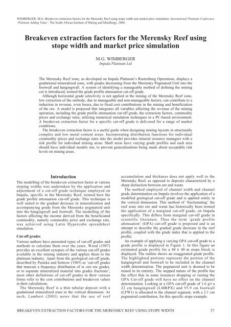
WIMBERGER, M.G. <strong>Breakeven</strong> <strong>extraction</strong> <strong>factors</strong> <strong>for</strong> <strong>the</strong> <strong>Merensky</strong> <strong>Reef</strong> <strong>using</strong> <strong>stope</strong> width and market price simulation. International Platinum Conference<br />
‘Platinum Adding Value’, The South African Institute of Mining and Metallurgy, 2004.<br />
<strong>Breakeven</strong> <strong>extraction</strong> <strong>factors</strong> <strong>for</strong> <strong>the</strong> <strong>Merensky</strong> <strong>Reef</strong> <strong>using</strong><br />
<strong>stope</strong> width and market price simulation<br />
Introduction<br />
The modelling of <strong>the</strong> breakeven <strong>extraction</strong> factor at various<br />
stoping widths was undertaken by <strong>the</strong> application and<br />
adjustment of a cut-off grade technique employed on<br />
Impala, specific to <strong>the</strong> <strong>Merensky</strong> <strong>Reef</strong>, termed here <strong>the</strong><br />
grade profile attenuation cut-off grade. This technique is<br />
well suited to <strong>the</strong> gradual decrease in mineralization and<br />
accompanying grade from <strong>the</strong> <strong>Merensky</strong> pegmatoid unit<br />
into <strong>the</strong> hangingwall and footwall. The modelling of <strong>the</strong><br />
<strong>factors</strong> affecting <strong>the</strong> income derived from <strong>the</strong> beneficiated<br />
commodity, namely commodity price and exchange rate,<br />
was achieved <strong>using</strong> Latin Hypercube spreadsheet<br />
simulation.<br />
Cut-off grades<br />
Various authors have presented types of cut-off grades and<br />
methods to calculate <strong>the</strong>m over <strong>the</strong> years. Wood (1997)<br />
provides an excellent synopsis of <strong>the</strong> various cut-off grades<br />
available in <strong>the</strong> mining industry and applies <strong>the</strong>m to <strong>the</strong><br />
platinum industry. Apart from <strong>the</strong> geological cut-off grade,<br />
described by Pasieka and Sotirow (1985) as ‘cut-off grades<br />
that truncate a frequency distribution of in situ ore grades,<br />
or to separate mineralized material into grades fractions’,<br />
most o<strong>the</strong>r definitions of cut-off grades in <strong>the</strong>ir various<br />
<strong>for</strong>ms refer to <strong>the</strong> cost contributions and breakeven values<br />
in <strong>the</strong>ir calculations.<br />
The <strong>Merensky</strong> <strong>Reef</strong> is a thin tabular deposit with a<br />
gradational mineralized zone in <strong>the</strong> vertical dimension. As<br />
such, Lambert (2003) notes that <strong>the</strong> use of reef<br />
M.G. WIMBERGER<br />
Impala Platinum Ltd<br />
The <strong>Merensky</strong> <strong>Reef</strong> zone, as developed on Impala Platinum’s Rustenburg Operations, displays a<br />
gradational mineralized zone, with grades decreasing from <strong>the</strong> <strong>Merensky</strong> Pegmatoid Unit into <strong>the</strong><br />
footwall and hangingwall. A system of identifying a manageable method of defining <strong>the</strong> mining<br />
cut is introduced, termed <strong>the</strong> grade profile attenuation cut-off grade.<br />
Although horizontal grade selectivity is not applied in <strong>the</strong> mining of <strong>the</strong> <strong>Merensky</strong> <strong>Reef</strong> zone,<br />
low <strong>extraction</strong> of <strong>the</strong> orebody, due to manageable and non-manageable <strong>factors</strong>, can contribute to a<br />
reduction in revenue, even losses, due to fixed cost contributions in <strong>the</strong> mining and beneficiation<br />
of <strong>the</strong> ore. A model is proposed that integrates all variables affecting <strong>the</strong> revenue of <strong>the</strong> mining<br />
operation, including <strong>the</strong> grade profile attenuation cut-off grade, <strong>the</strong> <strong>extraction</strong> <strong>factors</strong>, commodity<br />
prices and exchange rates, utilizing numerical simulation techniques in a PC-based environment.<br />
A breakeven <strong>extraction</strong> factor <strong>for</strong> a specific cut-off grade is delivered <strong>for</strong> a range of market<br />
conditions.<br />
The breakeven <strong>extraction</strong> factor is a useful guide when designing mining layouts in structurally<br />
complex and low metal content areas. Incorporating distribution functions <strong>for</strong> individual<br />
commodity prices and exchange rates into <strong>the</strong> model provides mineral resource managers with a<br />
risk profile <strong>for</strong> individual mining areas. Shaft areas have varying grade profiles and each area<br />
should have individual models run, to prevent generalizations being made about acceptable risk<br />
levels on mining areas.<br />
accumulation and thickness does not apply well to <strong>the</strong><br />
<strong>Merensky</strong> <strong>Reef</strong>, as opposed to deposits characterized by a<br />
sharp distinction between ore and waste.<br />
The method employed of channel width and channel<br />
grade determination on Impala involves <strong>the</strong> application of a<br />
modified geological cut-off grade and is applied solely in<br />
<strong>the</strong> vertical dimension. This method of ‘fractionating’ <strong>the</strong><br />
reef zone into ore and waste has historically been termed<br />
<strong>the</strong> application of a marginal cut-off grade, on Impala<br />
specifically. This differs from marginal cut-off grade in<br />
scientific literature. Thus <strong>the</strong> term ‘grade profile<br />
attenuation’ (GPA) cut-off grade is proposed and is an<br />
attempt to describe <strong>the</strong> gradual grade decrease in <strong>the</strong> reef<br />
profile, coupled with <strong>the</strong> grade index that is applied to <strong>the</strong><br />
profile.<br />
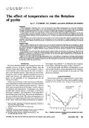
An example of applying a varying GPA cut-off grade to a<br />
grade profile is displayed in Figure 1. In this figure an<br />
estimated grade profile <strong>for</strong> a 40 x 40 m <strong>stope</strong> block is<br />
displayed. The outline shows an exaggerated grade profile.<br />
The highlighted portions represent <strong>the</strong> portion of <strong>the</strong><br />
hangingwall and footwall to be included in <strong>the</strong> channel<br />
width determination. The pegmatoid unit is deemed to be<br />
mined in its entirety. The stepped nature of <strong>the</strong> profile has<br />
<strong>the</strong> effect that in some instances dropping or raising <strong>the</strong><br />
GPA Cut-off grade will have no effect on <strong>the</strong> channel<br />
determination. Looking at a GPA cut-off grade of 1.6 g/t a<br />
22 cm hangingwall (LMRPX) and 55.9 cm footwall<br />
(LFW1) is allocated to <strong>the</strong> channel segment, with a 2.1 cm<br />
pegmatoid contribution, <strong>for</strong> this specific <strong>stope</strong> example.<br />
BREAKEVEN EXTRACTION FACTORS FOR THE MERENSKY REEF USING STOPE WIDTH 37
38<br />
Grade Profile Attenuation Cut-off Grade (g/t)<br />
4.0 3.9 3.8 3.7 3.6 3.5 3.4 3.3 3.2 3.1 3.0 2.9 2.8 2.7 2.6 2.5 2.4 2.3 2.2 2.1 2.0 1.9 1.8 1.7 1.6 1.5 1.4 1.3 1.2 1.1 1.0 0.9 0.8 0.7 0.6 0.5 0.4 0.3 0.2 0.1<br />
Channel<br />
Segment<br />
Grade (g/t)<br />
Channel<br />
Segment<br />
Width (cm)<br />
Rock<br />
Code<br />
LMRPX 10 0.23<br />
LMRPX 10 0.23<br />
LMRPX 10 0.18<br />
LMRPX 10 0.18<br />
LMRPX 10 0.27<br />
LMRPX 10 0.27<br />
LMRPX 10 0.55<br />
LMRPX 10 1.31<br />
LMRPX 10 3.14<br />
LMRPX 12 6.98<br />
LMRPG 2.1 40.66<br />
LFW 1 15.9 7.52<br />
LFW 1 10 5.41<br />
LFW 1 10 3.61<br />
LFW 1 10 2.64<br />
LFW 1 10 2.03<br />
LFW 1 10 1.64<br />
LFW 1 10 1.32<br />
LFW 1 10 0.75<br />
LFW 1 10 0.42<br />
LFW 1 10 0.25<br />
LFW 1 10 0.25<br />
LFW 1 10 0.24<br />
LFW 1 10 0.24<br />
LFW 1 10 0.18<br />
LFW 1 10 0.18<br />
LFW 1 10 0.21<br />
LFW 1 10 0.21<br />
LFW 1 10 0.17<br />
LFW 1 10 0.17<br />
LFW 1 10 0.23<br />
Figure 1. Exaggerated mean grade profile <strong>for</strong> <strong>Merensky</strong> ‘A’ <strong>Reef</strong>, showing <strong>the</strong> effect of applying an incremental grade profile attenuation<br />
index or ‘cut-off’ grade<br />
PLATINUM ADDING VALUE
Impala employs a minimum mining height of 80 cm on<br />
its conventional mining areas, with a maximum height of<br />
150 cm. Areas with a channel width of lower than 80 cm<br />
are increased to <strong>the</strong> minimum by an allowable overbreak<br />
parameter. Where <strong>the</strong> channel is in excess of 150 cm at a<br />
specific GPA cut-off grade, <strong>the</strong> channel parameters are<br />
reduced by an allowable underbreak factor. In all cases, <strong>the</strong><br />
<strong>Merensky</strong> pegmatoid unit is assumed to be mined in its<br />
entirety.<br />
Mining, beneficiation and <strong>extraction</strong> <strong>factors</strong><br />
Mining method<br />
Close to 98% of <strong>Merensky</strong> <strong>Reef</strong> areas are mined<br />
conventionally, on an up-dip breast mining method. Drives<br />
are developed in <strong>the</strong> footwall with a drive to reef middling<br />
averaging 25 m. Level spacings are in <strong>the</strong> order of<br />
45–50 m across <strong>the</strong> property, which results in back-lengths<br />
of approximately 310 m, given a reef dip of 9°. Raise line<br />
spacings are in <strong>the</strong> order of 120 m, and advance strike<br />
gullies are developed from <strong>the</strong> raise at an angle of<br />
approximately 15° above strike.<br />
Extraction factor<br />
The <strong>extraction</strong> factor, or sometimes called erroneously, <strong>the</strong><br />
<strong>extraction</strong> rate, is a lesser publicized figure which has<br />
enormous consequences <strong>for</strong> activities such as cost analysis<br />
and resource classifications. It is defined by Golenya (2002)<br />
as ‘that factor applied to an area of ground on a Half-Level<br />
and to individual blocks to estimate <strong>the</strong> mineable area after<br />
losses attributed to geological features, mining design and<br />
<strong>the</strong> ground control districts pillar configuration. The<br />
<strong>extraction</strong> factor is expressed as a percentage of what is<br />
estimated to be recoverable.’<br />
In terms of mining a reef or reef zone in <strong>the</strong> case of <strong>the</strong><br />
<strong>Merensky</strong> <strong>Reef</strong>, <strong>the</strong> <strong>extraction</strong> factor should be by all<br />
accounts divided into vertical <strong>extraction</strong> and horizontal<br />
<strong>extraction</strong> <strong>factors</strong>, since a three-dimensional block of ore is<br />
being removed. The vertical <strong>extraction</strong> factor presents a<br />
particular problem in definition on <strong>the</strong> <strong>Merensky</strong> <strong>Reef</strong>,<br />
since <strong>the</strong> channel estimates based on a specific GPA cut-off<br />
grade intrinsically defines <strong>the</strong> reef zone. A measure of <strong>the</strong><br />
overbreaks and underbreaks relative to issued parameters,<br />
resulting in a percentage channel dilution, is probably a<br />
better method to quantify <strong>extraction</strong> in <strong>the</strong> vertical sense.<br />
Stope design and <strong>the</strong> associated in-<strong>stope</strong> pillars<br />
consistently play a role in quantifying <strong>the</strong> (horizontal)<br />
<strong>extraction</strong> factor <strong>for</strong> a <strong>stope</strong> area, shaft, or project area.<br />
Pillar designs on conventional layouts rarely account <strong>for</strong><br />
more than 10% of <strong>the</strong> total area in question (L.G. Gardener,<br />
personal communication). Mechanized mining layouts,<br />
requiring higher <strong>stope</strong> widths, will alter this percentage,<br />
since larger spans would have to be supported, with a larger<br />
pillar design with depth a reasonable possibility.<br />
Geological features that contribute to losses or a decrease<br />
in <strong>the</strong> <strong>extraction</strong> factor, with <strong>the</strong> possible creation of white:<br />
areas, include <strong>the</strong> following:<br />
• Faults and shear zones—<strong>the</strong>se structural features cause<br />
ei<strong>the</strong>r reef losses through vertical displacement of <strong>the</strong><br />
reef, or create situations where large-scale collapses of<br />
<strong>the</strong> mining area occur. Such events, termed ‘falls of<br />
ground’, contribute negatively to earnings since<br />
rehabilitation costs are extremely high and conditions<br />
unsafe.<br />
• Dykes—two types of dykes occur across <strong>the</strong> property.<br />
Dolerite dykes can create losses due to <strong>the</strong> intrusion<br />
and associated horizontal displacement of <strong>the</strong> reef.<br />
Lamprophyre dykes are generally thinner than <strong>the</strong><br />
dolerites encountered, being in <strong>the</strong> order of tens of<br />
centimetres versus <strong>the</strong> metre-wide dolerite dykes, but<br />
can create severe ground control problems.<br />
Lamprophyre dykes exhibit extreme deterioration on<br />
exposure to water and air, and beam stability problems<br />
result when <strong>the</strong>se dykes advance in <strong>the</strong> direction of<br />
mining.<br />
• Potholes—<strong>the</strong> abrupt termination of available <strong>stope</strong><br />
face due to potholing causes losses of available ground.<br />
Depending of <strong>the</strong> size of <strong>the</strong> pothole, ei<strong>the</strong>r<br />
redevelopment is required, or complete abandonment<br />
of <strong>the</strong> <strong>stope</strong> or <strong>stope</strong>s. Pothole percentages vary across<br />
<strong>the</strong> property, and areas with high pothole frequencies in<br />
<strong>the</strong> order of 30 per cent of available ground are<br />
encountered.<br />
• Replacement pegmatoid zones—<strong>the</strong>se zones are<br />
generally associated with large-scale faulting and are<br />
believed to be related to <strong>the</strong> intrusion of late stage<br />
alteration fluids. The platinum content of <strong>the</strong> <strong>stope</strong> is<br />
generally unaffected, while <strong>the</strong> peak platinum marker<br />
tends to move marginally lower in <strong>the</strong> stratigraphy.<br />
Extraction rates can be negatively affected due to <strong>the</strong><br />
apparent lack of exposed reef, which would cause<br />
abandonment of stoping operations where replacement<br />
pegmatoid is encountered. Dilution percentages are<br />
also generally highest in <strong>the</strong>se areas as a result of<br />
excessive overbreak and underbreak, relative to <strong>the</strong><br />
stoping parameters.<br />
• Sills—if sills are developed sufficiently high in <strong>the</strong><br />
hangingwall, stoping may continue under certain<br />
parameter restrictions. However, massive <strong>stope</strong>,<br />
collapses have occurred in <strong>the</strong> past due to dead weight<br />
failure of insufficiently supported sills.<br />
• White areas—<strong>the</strong>se are areas created by <strong>the</strong> voluntary<br />
or involuntary abandonment of mining in a specific<br />
area. These white areas are in <strong>the</strong> most part being reinvestigated<br />
and opened up <strong>for</strong> mining again, albeit at a<br />
much higher cost than <strong>the</strong> initial mining operation<br />
would have cost. It is <strong>the</strong> percentage of ground that is<br />
left behind that makes <strong>the</strong> biggest impact on <strong>the</strong><br />
profitability of mining operations<br />
Costs<br />
Various costs are involved in <strong>the</strong> <strong>extraction</strong> and<br />
beneficiation of platinum group elements. These can be<br />
broadly classified into mining costs, processing costs,<br />
services costs, refineries costs, and selling and admin costs.<br />
Since this paper is not focused on a specific shaft or<br />
business unit within Impala, certain global assumptions<br />
about costs have been made.<br />
The costs used in <strong>the</strong> simulation model were based on<br />
projected costs <strong>for</strong> <strong>the</strong> current financial year (2003–2004),<br />
which in turn are summaries <strong>for</strong> both <strong>the</strong> <strong>Merensky</strong> and<br />
UG2. Tonnages are normalized to <strong>the</strong> target of achieving<br />
1.9 million ounces of PGEs.<br />
As with many industries, <strong>the</strong> cost of an operation or<br />
activity can be split into fixed and variable costs. Fixed<br />
costs are those costs that do not vary with an increase in<br />
production, and variable costs are those that do vary with an<br />
increase in production. Various classical economics<br />
textbooks refer to <strong>the</strong> fact that in <strong>the</strong> long term, <strong>the</strong>re are no<br />
fixed costs (Varian, 1992). Since <strong>the</strong> production projected<br />
BREAKEVEN EXTRACTION FACTORS FOR THE MERENSKY REEF USING STOPE WIDTH 39<br />
Ta<br />
Matr<br />
cutextra
40<br />
Figure 2. Layout of a typical <strong>Merensky</strong> mining layout with examples of structural features that affect <strong>the</strong> <strong>extraction</strong> factor<br />
in <strong>the</strong> model is based on an annual figure, <strong>the</strong> fixed costs<br />
are indeed fixed. Sunk costs are assumed to be those costs<br />
that have already been committed and cannot be recovered.<br />
However, confusion about <strong>the</strong> definition of what is fixed<br />
and sunk arises in a few economics texts (Baumol and<br />
Blinder, 1997). There is no distinction between <strong>the</strong>se two<br />
types of costs in this paper, and <strong>for</strong> matters of simplicity<br />
only fixed and variable costs are included. Avoidable costs,<br />
which do exist, are <strong>for</strong> all intents and purposes included in<br />
portions of fixed and variable costs, from historical<br />
projections of efficiencies.<br />
The total cost contribution to an activity is <strong>the</strong> sum of all<br />
<strong>the</strong> fixed and variable costs of all activities. Where this total<br />
cost is greater than <strong>the</strong> income generated from <strong>the</strong> sales of<br />
<strong>the</strong> platinum group metals, a loss is experienced.<br />
Conversely, a profit is yielded when <strong>the</strong> income generated<br />
exceeds <strong>the</strong> total cost of producing <strong>the</strong>se metals.<br />
<strong>Breakeven</strong> <strong>extraction</strong> factor determination<br />
The method of determining <strong>the</strong> breakeven <strong>extraction</strong> factor<br />
<strong>for</strong> a specific GPA cut-off grade involved two different<br />
models drawing on <strong>the</strong> same grade profiles, basic<br />
assumptions regarding metal splits, recoveries as well as<br />
modifying <strong>factors</strong> applied to <strong>the</strong> conversion of channel to<br />
mill widths and grades.<br />
The first method involved <strong>the</strong> construction of a profit-loss<br />
matrix, with static input variables, while <strong>the</strong> second method<br />
involved <strong>the</strong> dynamic modelling or simulation of <strong>the</strong><br />
variables, which provided a range of revenue outcomes,<br />
essentially reflecting best and worst case economic<br />
scenarios. Both methods are described in this report. A<br />
flowchart describing <strong>the</strong> steps common to both models,<br />
with <strong>the</strong> exception of <strong>the</strong> simulation of variables, is<br />
portrayed in Figure 3.<br />
An initial limiting factor on <strong>the</strong> model was that at each<br />
GPA cut-off grade, <strong>the</strong> kilograms produced must remain<br />
constant, at <strong>the</strong> maximum <strong>extraction</strong> factor applied. A<br />
decision was made not to maintain constant kilograms at all<br />
<strong>extraction</strong>s, since (a) plant kilogram fluctuations do occur,<br />
mainly as a result of a lack of tonnage from <strong>the</strong> plant, and<br />
(b) <strong>the</strong> models are designed merely as an initial<br />
investigative step, with <strong>the</strong> capacity to add on components<br />
based on requirements of management should it be<br />
required. The model could be criticized <strong>for</strong> being<br />
oversimplified, but <strong>the</strong> point is to provide some feel <strong>for</strong> <strong>the</strong><br />
character of <strong>the</strong> solutions and <strong>the</strong> sensitivity <strong>for</strong> various<br />
assumptions.<br />
Variables involved<br />
The following <strong>factors</strong> all play a pivotal rote in <strong>the</strong><br />
commercial viability of <strong>the</strong> mining of a mineral resource:<br />
• The grade of <strong>the</strong> ore being mined<br />
• The percentage splits and recoveries of <strong>the</strong> metals to be<br />
recovered from <strong>the</strong> ore<br />
• The cost of mining <strong>the</strong> ore<br />
• The cost of milling <strong>the</strong> ore<br />
• The cost of processing <strong>the</strong> milled ore<br />
• The cost of refining <strong>the</strong> metal recovered from <strong>the</strong><br />
processed matte<br />
• The cost of marketing and selling <strong>the</strong> products<br />
• The prevailing and long-term prospects of <strong>the</strong><br />
commodity prices<br />
• The prevailing and medium-term prospects of <strong>the</strong><br />
exchange rate, if <strong>the</strong> metal price is based on a <strong>for</strong>eign<br />
currency.<br />
These <strong>factors</strong> as well as <strong>the</strong> correction <strong>factors</strong> applied to<br />
convert from channel to mill, and <strong>the</strong> kilogram to ounce<br />
conversion factor were built into a spreadsheet model. For<br />
every GPA cut-off grade and <strong>extraction</strong> factor combination,<br />
a total cost and turnover figure was calculated, with <strong>the</strong><br />
resultant revenue generated. Positive revenues reflect a<br />
profitable scenario, whereas negative revenues <strong>for</strong> a<br />
particular cut-off grade and <strong>extraction</strong> factor combination<br />
reflect a loss.<br />
Static model<br />
The static model involved <strong>the</strong> specific commodity prices<br />
and exchange rates at each <strong>extraction</strong> factor and cut-off<br />
grade combination. Results of <strong>the</strong> each run were reflected<br />
in a summary profit-loss matrix, where a conditional<br />
indicator ‘PROFIT’ was returned <strong>for</strong> revenues greater than<br />
zero, and ‘LOSS’ returned <strong>for</strong> revenue less than zero. A<br />
random selection of three profit-loss matrixes is shown in<br />
Table I.<br />
PLATINUM ADDING VALUE
Figure 3. Flowchart outlining <strong>the</strong> basic steps involved in <strong>the</strong> determination of <strong>the</strong> breakeven <strong>extraction</strong> factor<br />
at varying GPA cut-off grades<br />
The profit-loss matrix portrayed in Table I, shows a<br />
‘boundary’ between <strong>the</strong> two indicator categories, which<br />
moves from <strong>the</strong> top leftmost quadrant in an apparent wave,<br />
to <strong>the</strong> bottom rightmost quadrant, as market conditions<br />
improve.<br />
The profit-loss matrices work well as a motivational tool<br />
<strong>for</strong> resources managers trying to improve <strong>the</strong> <strong>extraction</strong><br />
factor and optimization of an orebody. However, <strong>the</strong> detail<br />
behind <strong>the</strong> model is cumbersome, <strong>the</strong> various iterations<br />
necessary with <strong>the</strong> volatility of <strong>the</strong> market make long-term<br />
range assessment difficult, and <strong>the</strong> output is qualitative but<br />
indicator filtered, with no hint of relative highs or lows.<br />
Risk analysis and simulation<br />
A need to quantify <strong>the</strong> ranges in revenue due to market<br />
fluctuations, as well as to identify <strong>the</strong> contributors to <strong>the</strong><br />
greatest variation in revenue, was identified. Risk<br />
management or analysis software is one method to this<br />
achieve this goal. Palisade Corporation’s risk analysis suite,<br />
@RISK 4.5, was used due to <strong>the</strong> fact that <strong>the</strong> base model<br />
used in <strong>the</strong> static case analysis could be incorporated<br />
without modification.<br />
The word risk relates to uncertainty in <strong>the</strong> outcome of an<br />
event or decision, and in <strong>the</strong> case of <strong>the</strong> revenue calculation<br />
model, relates to <strong>the</strong> variability to <strong>the</strong> variables involved in<br />
<strong>the</strong> calculation of <strong>the</strong> revenue at varying cut-off grades and<br />
<strong>extraction</strong> <strong>factors</strong>. The range of outcomes or results is<br />
associated with probability levels. The type of risk involved<br />
in <strong>the</strong> model creation is subjective risk with <strong>the</strong> best<br />
estimate being gained from personal knowledge and filtered<br />
in<strong>for</strong>mation ga<strong>the</strong>ring techniques<br />
The technique used by @RISK is quantitative, usually<br />
referred to as simulation. Simulation is <strong>the</strong> term used where<br />
a model, such as <strong>the</strong> Revenue model developed in Excel, is<br />
calculated many times, with changing variable values, with<br />
<strong>the</strong> aim of getting a complete representation of all <strong>the</strong><br />
possible combinations of cut-off grades and <strong>extraction</strong><br />
<strong>factors</strong>.<br />
Distribution sampling<br />
Latin Hypercube is a relatively recent development in<br />
sampling techniques and was first proposed by McKay<br />
et al. (1979). It is a stratified sampling technique with a<br />
random selection of each stratum within <strong>the</strong> sampled<br />
distribution. With Latin Hypercube sampling, sample<br />
values are randomly shuffled among different variables. As<br />
sampling is <strong>for</strong>ced to represent values in each interval, it is<br />
<strong>for</strong>ced to recreate <strong>the</strong> input probability distribution. A<br />
representation of <strong>the</strong> stratification system employed by<br />
Latin Hypercube sampling is shown in Figure 4. Latin<br />
Hypercube sampling does not resample values already<br />
sampled, and <strong>the</strong> number of stratifications is equal to <strong>the</strong><br />
number of iterations. Thus, if a distribution with 200<br />
discreet values is sampled, with 1 000 iterations, some<br />
values may be sampled more than once, depending on <strong>the</strong><br />
probability attached to <strong>the</strong> value.<br />
Each variable chosen in <strong>the</strong> model is considered to be<br />
independent, and modelled accordingly, preventing any<br />
unnecessary, and potentially conf<strong>using</strong> correlation between<br />
variables. With sufficient iterations, situations where<br />
variable are indeed correlated might in fact be sampled as<br />
such, without defined correlation. Low probability variables<br />
are catered <strong>for</strong> in <strong>the</strong> sampling process by <strong>the</strong> implicit<br />
stratification across <strong>the</strong> entire distribution.<br />
Distribution sampling occurs in @RISK through <strong>the</strong><br />
allocation of a distribution descriptor function in <strong>the</strong> model.<br />
Two types of distribution functions were used in <strong>the</strong> model,<br />
viz. RiskHistogrm and RiskUni<strong>for</strong>m.<br />
BREAKEVEN EXTRACTION FACTORS FOR THE MERENSKY REEF USING STOPE WIDTH 41
Table I<br />
Profit loss matrix <strong>for</strong> various GPS cut-off grades and <strong>extraction</strong> <strong>factors</strong> at a Pt price of $865/oz, Pd price of $239/oz, Rh price of $520/oz, Ru<br />
price of $42/oz, Ir price of $85/oz, Au price of $409/oz and exchange rate of R7.16$<br />
GPA Cut-off Extraction factor<br />
grade (g/t) 100% 90% 80% 70% 60% 50% 40% 30% 20% 10%<br />
4.0 Profit Profit Profit Profit Profit Profit Profit Profit Loss Loss<br />
3.9 Profit Profit Profit Profit Profit Profit Profit Profit Loss Loss<br />
3.8 Profit Profit Profit Profit Profit Profit Profit Profit Loss Loss<br />
3.7 Profit Profit Profit Profit Profit Profit Profit Profit Loss Loss<br />
3.6 Profit Profit Profit Profit Profit Profit Profit Profit Loss Loss<br />
3.5 Profit Profit Profit Profit Profit Profit Profit Profit Loss Loss<br />
3.4 Profit Profit Profit Profit Profit Profit Profit Profit Loss Loss<br />
3.3 Profit Profit Profit Profit Profit Profit Profit Profit Loss Loss<br />
3.2 Profit Profit Profit Profit Profit Profit Profit Profit Loss Loss<br />
3.1 Profit Profit Profit Profit Profit Profit Profit Profit Loss Loss<br />
3.0 Profit Profit Profit Profit Profit Profit Profit Profit Loss Loss<br />
2.9 Profit Profit Profit Profit Profit Profit Profit Profit Loss Loss<br />
2.8 Profit Profit Profit Profit Profit Profit Profit Profit Loss Loss<br />
2.7 Profit Profit Profit Profit Profit Profit Profit Profit Loss Loss<br />
2.6 Profit Profit Profit Profit Profit Profit Profit Profit Loss Loss<br />
2.5 Profit Profit Profit Profit Profit Profit Profit Profit Loss Loss<br />
2.4 Profit Profit Profit Profit Profit Profit Profit Profit Loss Loss<br />
2.3 Profit Profit Profit Profit Profit Profit Profit Profit Loss Loss<br />
2.2 Profit Profit Profit Profit Profit Profit Profit Profit Loss Loss<br />
2.1 Profit Profit Profit Profit Profit Profit Profit Profit Loss Loss<br />
2.0 Profit Profit Profit Profit Profit Profit Profit Profit Loss Loss<br />
1.9 Profit Profit Profit Profit Profit Profit Profit Loss Loss Loss<br />
1.8 Profit Profit Profit Profit Profit Profit Profit Loss Loss Loss<br />
1.7 Profit Profit Profit Profit Profit Profit Profit Loss Loss Loss<br />
1.6 Profit Profit Profit Profit Profit Profit Profit Loss Loss Loss<br />
1.5 Profit Profit Profit Profit Profit Profit Profit Loss Loss Loss<br />
1.4 Profit Profit Profit Profit Profit Profit Profit Loss Loss Loss<br />
1.3 Profit Profit Profit Profit Profit Profit Profit Loss Loss Loss<br />
1.2 Profit Profit Profit Profit Profit Profit Profit Loss Loss Loss<br />
1.1 Profit Profit Profit Profit Profit Profit Profit Loss Loss Loss<br />
1.0 Profit Profit Profit Profit Profit Profit Profit Loss Loss Loss<br />
0.9 Profit Profit Profit Profit Profit Profit Loss Loss Loss Loss<br />
0.8 Profit Profit Profit Profit Profit Profit Loss Loss Loss Loss<br />
0.7 Profit Profit Profit Profit Profit Profit Loss Loss Loss Loss<br />
0.6 Profit Profit Profit Profit Profit Loss Loss Loss Loss Loss<br />
0.5 Profit Profit Profit Profit Profit Loss Loss Loss Loss Loss<br />
0.4 Profit Profit Profit Profit Profit Loss Loss Loss Loss Loss<br />
0.3 Profit Profit Profit Loss Loss Loss Loss Loss Loss Loss<br />
0.2 Loss Loss Loss Loss Loss Loss Loss Loss Loss Loss<br />
0.1 Loss Loss Loss Loss Loss Loss Loss Loss Loss Loss<br />
42<br />
Cumulative<br />
probability<br />
distribution<br />
stratified into<br />
five intervals<br />
1.0<br />
.9<br />
.8<br />
.7<br />
.6<br />
.5<br />
.4<br />
.3<br />
.2<br />
.1<br />
0<br />
Minimum<br />
Distribution<br />
Value<br />
Value Sampled<br />
Maximum<br />
Distribution<br />
Value<br />
Figure 4. Sampling of a cumulative distribution curve <strong>using</strong> Latin Hypercube sampling<br />
(modified from Palisade Software users, manual, 2003)<br />
PLATINUM ADDING VALUE
The <strong>for</strong>m of <strong>the</strong> RiskHistogrm function is:<br />
= RiskHistogrm (minimum,maximum,{p.1,p.2,...,p.n})<br />
which describes a histogram distribution with a range<br />
defined by <strong>the</strong> minimum and maximum values, divided into<br />
n classes, each class having a weighting p. Each weight is<br />
relative, thus weightings do not have to add up 100% with<br />
<strong>the</strong> normalizing achieved by summing all individual<br />
weights and dividing each weight by this summation.<br />
The RiskUni<strong>for</strong>m distribution function is described by:<br />
= RiskUni<strong>for</strong>m (minimum,maximum)<br />
which specifies a uni<strong>for</strong>m probability distribution with<br />
every value across <strong>the</strong> range having an equal likelihood of<br />
occurrence.<br />
The RiskHistogrm function used <strong>for</strong> <strong>the</strong> above variables is as follows:<br />
USdol2Rand RiskHistogrm (6,12.5,(0, 17, 34, 71, 173, 125, 49, 41,<br />
50, 81, 49, 57, 26, 8))<br />
Ptdoloz RiskHistogrm (400, 910, (0, 0.8, 16, 23, 19, 22, 24, 24,<br />
8, 7, 9, 18, 34, 22, 24, 45, 22, 27, 36, 51, 37, 30, 18, 17,<br />
13, 11, 25, 24, 23, 29, 18, 8, 9, 6, 4, 10, 11, 3.1, 2, 2.1,<br />
3, 0, 0, 0, 0, 0, 0, 0, 0))<br />
Audoloz RiskHistogrm (200, 430, (0, 0, 0, 0, 0, 0, 18, 111, 97,<br />
39, 49, 38, 97, 56, 22, 42, 56, 34, 36, 24, 13, 12, 0, 0))<br />
Rhdoloz RiskUni<strong>for</strong>m (400, 500)<br />
Pddoloz RiskHistogrm (150, 1075, (4, 54, 84, 45, 42, 41, 8, 92,<br />
61, 72, 34, 13, 25, 27, 3, 2, 2, 6, 7, 14, 14, 13, 8, 7, 4, 9,<br />
7, 4, 2, 2, 1, 0, 1, 7, 4, 2, 8, 13, 2))<br />
Note that <strong>the</strong> rhodium price uses a RiskUni<strong>for</strong>m Function, with minimum<br />
and maximum values of 400 and 500 US Dollars per ounce. Ru<strong>the</strong>nium<br />
and iredium were included in <strong>the</strong> model at static prices of $41/oz and<br />
$87/oz repectively<br />
<strong>Breakeven</strong> analysis<br />
Each combination of <strong>extraction</strong> rate and GPA cut-off grade<br />
was simulated in @RISK, with <strong>the</strong> variables. Considering<br />
that <strong>the</strong> model was constrained between GPA cut-off grades<br />
of 2.0 and 0.1 g/t, 200 discreet revenue distributions were<br />
produced, an example of which is contained in Figure 5.<br />
Revenue is expressed in R millions.<br />
The shape of <strong>the</strong> probability distribution has a slight<br />
positive skewness, due to <strong>the</strong> effect of <strong>the</strong> distribution<br />
shape of <strong>the</strong> commodity prices and exchange rates. This is<br />
expected to be <strong>the</strong> norm of most revenue distribution plots,<br />
Revenue (Rands)<br />
6000<br />
5000<br />
4000<br />
3000<br />
2000<br />
1000<br />
0<br />
-1000<br />
-2000<br />
100% 90% 80% 70% 60% 50% 40% 30% 20% 10%<br />
Extraction Factor<br />
as Cashin et al. (1999) points out, ‘price slumps last longer<br />
than price booms’.<br />
The process of determining <strong>the</strong> breakeven <strong>extraction</strong><br />
factor at a GPA cut-off grade analysing <strong>the</strong> revenue at<br />
varying <strong>extraction</strong> <strong>factors</strong>, while keeping <strong>the</strong> GPA cut-off<br />
grade constant. Since a range of probable revenue values is<br />
produced <strong>for</strong> each combination, <strong>the</strong> mean, 95th and 5th<br />
percentile as well as one standard deviation from <strong>the</strong> mean<br />
were chosen to regress and determine <strong>the</strong> breakeven<br />
<strong>extraction</strong> factor, or likewise <strong>the</strong> breakeven cut-off grade<br />
<strong>for</strong> a specific <strong>extraction</strong> factor.<br />
Ranges of revenue based on specific combinations of cutoff<br />
grade and <strong>extraction</strong> factor are shown in<br />
Figures 6(a)-(b) * and 7 †. All charts showing <strong>the</strong> revenue at<br />
a specific cut-off grade show a negative slope, or more<br />
specifically a decrease in revenue with a decrease in<br />
<strong>extraction</strong> factor. The situation changes radically at a cutoff<br />
grade of 0.3 to 0.1 g/t, where <strong>the</strong> range of revenue<br />
values from <strong>the</strong> 5th percentile to 1 standard deviation of <strong>the</strong><br />
mean show positive slopes, with a decrease in <strong>the</strong><br />
<strong>extraction</strong> rate. This means that less loss is made if less is<br />
mined, when market conditions are unfavourable.<br />
*(Constant GPA cut-off grade) †(Constant <strong>extraction</strong> factor)<br />
X
A point of inflection is evidenced in Figure 7 depicting <strong>the</strong><br />
range of revenues based on a specific GPA cut-off grade,<br />
due to a marked increase in defined channel width when<br />
decreasing <strong>the</strong> cut-off grade.<br />
Consolidation of results<br />
Regression and analysis of <strong>the</strong> data from <strong>the</strong> simulations<br />
enabled an <strong>extraction</strong> factor to be determined <strong>for</strong> revenue<br />
return of zero. This is taken to be <strong>the</strong> breakeven <strong>extraction</strong><br />
factor <strong>for</strong> a specific GPA cut-off grade. Results from this<br />
analysis are contained in Table II, and graphed in Figure 8.<br />
Due to <strong>the</strong> combination of high stoping heights and high<br />
associated costs, along with simulated market conditions,<br />
certain of <strong>the</strong> combinations regression return breakeven<br />
<strong>extraction</strong> <strong>factors</strong> in excess of 100%. These are removed<br />
from <strong>the</strong> results, since <strong>the</strong>se situations will always be mined<br />
at a comparative loss. It must be noted that <strong>the</strong> denotation<br />
of <strong>the</strong> -5% and -25% does not refer to negative per cent<br />
<strong>extraction</strong> <strong>factors</strong>, but <strong>the</strong> percentiles with unfavourable<br />
economic conditions, i.e. low exchange rates and low<br />
commodity prices.<br />
Under all market conditions, a decrease in <strong>the</strong> breakeven<br />
<strong>extraction</strong> factor occurs with an increase in <strong>the</strong> GPA cut-off<br />
grade. The variance in <strong>the</strong> breakeven <strong>extraction</strong> factor at<br />
varying market conditions (-5th percentile represent <strong>the</strong><br />
worst case scenario while <strong>the</strong> 95th percentile <strong>the</strong> best case<br />
scenario) decreases with an increase in <strong>the</strong> GPA cut-off<br />
grade.<br />
Variances between <strong>the</strong> mean value and <strong>the</strong> 95th<br />
44<br />
Revenue (Rands)<br />
Revenue (Rands)<br />
0<br />
-1000<br />
-2000<br />
-3000<br />
-4000<br />
-5000<br />
-6000<br />
-7000<br />
-8000<br />
100% 80% 60% 40% 20%<br />
Extraction Factor<br />
Mean, +1/-1 Standard Deviation<br />
+ 95%, - 5%<br />
Figure 6(b). Range of revenue values at varying commodity prices and exchange rates at 0.1 g/t GPA cut-off grade<br />
3000<br />
1000<br />
-1000<br />
-3000<br />
-5000<br />
-7000<br />
2 1.8 1.6 1.4 1.2 1 0.8 0.6 0.4 0.2<br />
GPA Cut-off Grade )g/t)<br />
Mean, +1/-1 Standard Deviation<br />
+ 95%, - 5%<br />
Figure 7. Range of revenue values at a 50% <strong>extraction</strong> factor with varying commodity prices and exchange rates<br />
percentile breakeven <strong>extraction</strong> factor are in <strong>the</strong> order of 20<br />
to 10 per cent, while between that of <strong>the</strong> mean and <strong>the</strong> 5th<br />
percentile ranges from 65 to 35%.<br />
Thus, at low commodity prices and a strong local<br />
currency to <strong>the</strong> US Dollar, revenue losses per mining area<br />
easily occur, should ground be abandoned due to ground<br />
conditions or bad mining practices. Given that <strong>the</strong> low-end<br />
members of <strong>the</strong> variables modelled have occurred in <strong>the</strong><br />
past three years, and that no certainty in markets exists,<br />
loss-making stoping is a distinct possibility, with low<br />
<strong>extraction</strong> of ground, or low channel grades, or both.<br />
Impala mines <strong>the</strong> <strong>Merensky</strong> <strong>Reef</strong> at an average <strong>extraction</strong><br />
factor of 64% at a GPA cut-off grade of 1.5 g/t, which is<br />
above all breakeven <strong>extraction</strong> <strong>factors</strong>, except at <strong>the</strong> -5th<br />
percentile value, representing <strong>the</strong> most negative economic<br />
conditions. Losses might be incurred per stoping area if <strong>the</strong><br />
<strong>extraction</strong> of ground drops below a mean value of 37%. If<br />
mining had to continue at <strong>the</strong> present <strong>extraction</strong> factor,<br />
profits could be achieved with an increase in <strong>the</strong> GPA cutoff<br />
grade, and <strong>the</strong> resultant dropping of channel width. The<br />
alternative is to maintain <strong>the</strong> stoping height and improve <strong>the</strong><br />
<strong>extraction</strong> of ore.<br />
Conclusions and recommendations<br />
The cut-off grade philosophy introduced is unique in that<br />
no economics play a part in its construction, and it is<br />
coupled directly to <strong>the</strong> minimum and maximum stoping<br />
heights by overbreak and underbreak parameters.<br />
PLATINUM ADDING VALUE
GPA cut-off -5% Perc <strong>extraction</strong> -25% Perc <strong>extraction</strong> Mean <strong>extraction</strong> +75% Perc <strong>extraction</strong> +95% Perc <strong>extraction</strong><br />
(g/t) factor factor factor factor factor<br />
0.1<br />
0.2 74<br />
0.3 80 55 44<br />
0.4 67 48 38<br />
0.5 98 60 44 35<br />
0.6 92 56 41 33<br />
0.7 80 52 38 31<br />
0.8 76 50 37 30<br />
0.9 94 72 47 35 28<br />
1.0 86 66 44 33 27<br />
1.1 82 65 43 32 26<br />
1.2 80 63 42 31 26<br />
1.3 77 59 39 30 25<br />
1.4 75 58 39 30 25<br />
1.5 70 55 37 28 24<br />
1.6 66 52 36 27 22<br />
1.7 64 50 35 27 22<br />
1.8 63 51 35 26 22<br />
1.9 59 48 33 25 21<br />
2.0 57 46 32 25 21<br />
Breakage <strong>extraction</strong> factor<br />
Table II<br />
Showing <strong>the</strong> breakeven <strong>extraction</strong> factor (in per cent) based on varying GPA cut-off grades<br />
100<br />
80<br />
60<br />
40<br />
20<br />
0<br />
0 0.5 1 1.5 2<br />
GPA Cut-off (g/t)<br />
Figure 8. Summary of breakeven <strong>extraction</strong> factor at various GPA cut-off grades <strong>for</strong> varying market conditions<br />
Increasing <strong>the</strong> stoping height has <strong>the</strong> indirect effect of a<br />
lowering of <strong>the</strong> GPA cut-off grade. This situation can result<br />
in losses should market conditions be unfavourable, or<br />
<strong>extraction</strong> of <strong>the</strong> ground in a <strong>stope</strong> be insufficient to cover<br />
<strong>the</strong> total fixed and variable costs associated with <strong>the</strong> mining<br />
and beneficiation of that ore.<br />
Cost contributions and market prices <strong>for</strong>m <strong>the</strong> overall<br />
basis of base case feasibilities. The ground able to be<br />
extracted from a project area must be able to cover <strong>the</strong> costs<br />
of <strong>extraction</strong> and beneficiation. Total optimization of a<br />
mine would involve achieving this aim with each and every<br />
<strong>stope</strong>.<br />
Shaft mine areas have considerable amounts of data<br />
associated with geological structures and underground<br />
sampling. Mining layouts are generally decided upon far in<br />
advance. With <strong>the</strong> advent of unfavourable economic<br />
conditions, <strong>the</strong> temptation to increase tonnage output by<br />
widening <strong>the</strong> stoping height, or decreasing <strong>the</strong> GPA cut-off<br />
grade, should be resisted. Ra<strong>the</strong>r, mining more panels, at<br />
-5% Perc<br />
<strong>extraction</strong><br />
factor<br />
-25% Perc<br />
<strong>extraction</strong><br />
factor<br />
Mean<br />
<strong>extraction</strong><br />
factor<br />
+75% Perc<br />
<strong>extraction</strong><br />
factor<br />
+95% Perc<br />
<strong>extraction</strong><br />
factor<br />
comparable mining parameters, should be implemented to<br />
increase tonnage with no negative effect on grade, and<br />
accordingly on <strong>the</strong> revenues.<br />
The practice of leaving ground behind due to difficult<br />
mining, poor advances or stoping inefficiencies is<br />
manageable, and requires close monitoring. Returning to<br />
previously mining areas to remove scattered remnants of<br />
ground leads to costly re-equipping and removal of ore.<br />
Cost analyses must take all <strong>factors</strong> into consideration,<br />
including processing costs and o<strong>the</strong>r overheads, as well as<br />
prevailing market conditions. White area mining as<br />
practised on Impala would benefit from simulation<br />
modelling, albeit with tighter constraints on <strong>the</strong> variables,<br />
to determine <strong>the</strong> optimal mining cut based on cut-off grade<br />
models.<br />
The breakeven <strong>extraction</strong> factor generated <strong>for</strong> various<br />
GPA cut-off grades must be viewed in relation to <strong>the</strong> mine<br />
design and its related pillar losses and structural domains.<br />
The generation of white areas creates short- to medium-<br />
BREAKEVEN EXTRACTION FACTORS FOR THE MERENSKY REEF USING STOPE WIDTH 45
term drops in <strong>the</strong> <strong>extraction</strong> factor. The reinvestigation and<br />
mining of <strong>the</strong>se areas should be prompted by positive<br />
changes in <strong>the</strong> economic climate, and or changes to <strong>the</strong><br />
GPA cut-off grade.<br />
46<br />
References and fur<strong>the</strong>r reading<br />
BAUMOL, W.J. and BLINDER, A.S. Microeconomics:<br />
Principles and Policy. 7th Edition. Dryden. 1997.<br />
CASHIN, P., MCDERMOTT, C.J., and SCOTT, A. The<br />
myth of co-moving commodity prices. Reserve Bank<br />
of New Zealand Discussion Paper Series. G99/9.<br />
1999.<br />
CILLIERS, B. Generalized geological succession at Impala<br />
Platinum. (Unpub. company report). Rustenburg.<br />
1998.<br />
CRUNDWELL, I.H. Introduction to Geostatistics on<br />
Impala Platinum. (Unpub. company report).<br />
Rustenburg. 2000<br />
GOLENYA, F. Standard Procedures <strong>for</strong> <strong>the</strong> Reporting of<br />
<strong>the</strong> Mines Mineral Resources and Reserves.<br />
Addendum 2. MRD/11/03 (Unpub. company report).<br />
Rustenburg. 2003.<br />
IMAN, R.L. and CONOVER, W.J. Small Sample<br />
Sensitivity Analysis Techniques <strong>for</strong> Computer<br />
Models, with an Application to Risk Assessment.<br />
Communications in Statistics: Theory and Methods A<br />
vol. 9, 1980. pp. 1749–1874.<br />
LAMBERT, S. Something <strong>for</strong> nothing? An unconventional<br />
approach to extracting three-dimensional grade<br />
in<strong>for</strong>mation from two-dimensional estimation of thin,<br />
tabular reef deposits. APCOM 2003, SAIMM. 2003.<br />
pp. 1–6.<br />
LANE, K. The economic definition of ore. Cut-off grades in<br />
<strong>the</strong>ory and practice. Mining Journal Books. London.<br />
1998.<br />
McKAY, M.D., CONOVER, W.J., and BECKMAN, R.J. A<br />
Comparison of Three Methods <strong>for</strong> Selecting Values of<br />
Input Variables in <strong>the</strong> Analysis of Output from a<br />
Computer Code. Technometrics vol. 21, 1979.<br />
pp. 239–245.<br />
PALISADE CORPORATION (2002) @ Risk 4.5 Users<br />
Manual. New York.<br />
PASIEKA, A.R. and SOTIROW, G.V. Planning and<br />
Operational Cut-off grades based on computerized net<br />
present value and net cash flow. CIM Bull. 1985.<br />
SCHOUSTRA, R.P., KINLOCH, E.D., and LEE, C.A. A<br />
Short Geological Review of <strong>the</strong> Bushveld Complex.<br />
Platinum Metals Review. Johnson Mat<strong>the</strong>y. vol. 44,<br />
no. 1, 2000. pp. 33–39.<br />
SOLOW, R.M. and WAN, F.Y. Extraction costs in <strong>the</strong><br />
<strong>the</strong>ory of exhaustible resources. Bell Journal of<br />
Economics vol.7, no. 2, 1976. pp. 359–370.<br />
STANVLIET, D.F. and HAMBIDES, F.R. Standard<br />
Sampling Procedure of Impala Platinum Limited<br />
(Unpub. company report). Rustenburg. 2001.<br />
VARIAN, H.R. Microeconomic Analysis, 3rd Edition,<br />
Norton. 1992.<br />
VILJOEN, M.J. A review of regional variations in facies<br />
and grade distribution of <strong>the</strong> <strong>Merensky</strong> <strong>Reef</strong>, Western<br />
Bushveld Complex with some mining implications.<br />
XVth CMMI Congress. Johannesburg. SAIMM. vol.<br />
3, 1994. pp. 183–194<br />
WOOD, J.A. An investigation into <strong>the</strong> impact of Cut-off<br />
grades on <strong>the</strong> risks associated with mineral<br />
exploitation in <strong>the</strong> South African platinum industry.<br />
(Unpub. M.Sc dissertation). Witwatersrand<br />
University. Johannesburg. 1997.<br />
PLATINUM ADDING VALUE