First Semester in Numerical Analysis with Julia, 2020a

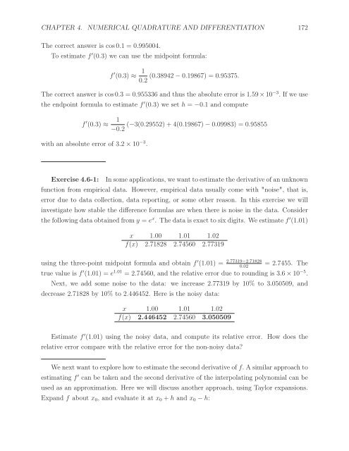
CHAPTER 4. NUMERICAL QUADRATURE AND DIFFERENTIATION 172
The correct answer is cos 0.1 =0.995004.
To estimate f ′ (0.3) we can use the midpoint formula:
f ′ (0.3) ≈ 1 (0.38942 − 0.19867) = 0.95375.
0.2
The correct answer is cos 0.3 =0.955336 and thus the absolute error is 1.59 × 10 −3 . If we use
the endpoint formula to estimate f ′ (0.3) we set h = −0.1 and compute
f ′ (0.3) ≈ 1 (−3(0.29552) + 4(0.19867) − 0.09983) = 0.95855
−0.2
with an absolute error of 3.2 × 10 −3 .
Exercise 4.6-1: In some applications, we want to estimate the derivative of an unknown
function from empirical data. However, empirical data usually come with "noise", that is,
error due to data collection, data reporting, or some other reason. In this exercise we will
investigate how stable the difference formulas are when there is noise in the data. Consider
the following data obtained from y = e x . The data is exact to six digits. We estimate f ′ (1.01)
x 1.00 1.01 1.02
f(x) 2.71828 2.74560 2.77319
using the three-point midpoint formula and obtain f ′ (1.01) = 2.77319−2.71828 =2.7455. The
0.02
true value is f ′ (1.01) = e 1.01 =2.74560, and the relative error due to rounding is 3.6 × 10 −5 .
Next, we add some noise to the data: we increase 2.77319 by 10% to 3.050509, and
decrease 2.71828 by 10% to 2.446452. Here is the noisy data:
x 1.00 1.01 1.02
f(x) 2.446452 2.74560 3.050509
Estimate f ′ (1.01) using the noisy data, and compute its relative error. How does the
relative error compare with the relative error for the non-noisy data?
We next want to explore how to estimate the second derivative of f. A similar approach to
estimating f ′ can be taken and the second derivative of the interpolating polynomial can be
used as an approximation. Here we will discuss another approach, using Taylor expansions.
Expand f about x 0 , and evaluate it at x 0 + h and x 0 − h: