First Semester in Numerical Analysis with Julia, 2020a

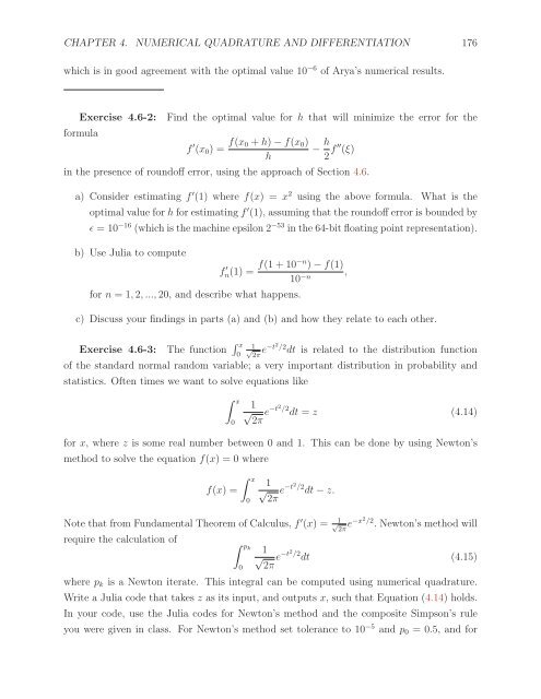
CHAPTER 4. NUMERICAL QUADRATURE AND DIFFERENTIATION 176
which is in good agreement with the optimal value 10 −6 of Arya’s numerical results.
Exercise 4.6-2: Find the optimal value for h that will minimize the error for the
formula
f ′ (x 0 )= f(x 0 + h) − f(x 0 )
− h h 2 f ′′ (ξ)
in the presence of roundoff error, using the approach of Section 4.6.
a) Consider estimating f ′ (1) where f(x) =x 2 using the above formula. What is the
optimal value for h for estimating f ′ (1), assuming that the roundoff error is bounded by
ɛ =10 −16 (which is the machine epsilon 2 −53 in the 64-bit floating point representation).
b) Use Julia to compute
f n(1) ′ = f(1+10−n ) − f(1)
,
10 −n
for n =1, 2, ..., 20, and describe what happens.
c) Discuss your findings in parts (a) and (b) and how they relate to each other.
Exercise 4.6-3: The function ∫ x
√1
0 2π
e −t2 /2 dt is related to the distribution function
of the standard normal random variable; a very important distribution in probability and
statistics. Often times we want to solve equations like
∫ x
0
1
√
2π
e −t2 /2 dt = z (4.14)
for x, where z is some real number between 0 and 1. This can be done by using Newton’s
method to solve the equation f(x) =0where
f(x) =
∫ x
0
1
√
2π
e −t2 /2 dt − z.
Note that from Fundamental Theorem of Calculus, f ′ (x) = 1 √
2π
e −x2 /2 . Newton’s method will
require the calculation of
∫ pk
0
1
√
2π
e −t2 /2 dt (4.15)
where p k is a Newton iterate. This integral can be computed using numerical quadrature.
Write a Julia code that takes z as its input, and outputs x, such that Equation (4.14) holds.
In your code, use the Julia codes for Newton’s method and the composite Simpson’s rule
you were given in class. For Newton’s method set tolerance to 10 −5 and p 0 =0.5, and for