SCOTT RIVER BASIN GRANITIC SEDIMENT STUDY ... - KRISWeb
SCOTT RIVER BASIN GRANITIC SEDIMENT STUDY ... - KRISWeb
SCOTT RIVER BASIN GRANITIC SEDIMENT STUDY ... - KRISWeb

Create successful ePaper yourself
Turn your PDF publications into a flip-book with our unique Google optimized e-Paper software.
Scanned for KRIS<br />
November<br />
1990<br />
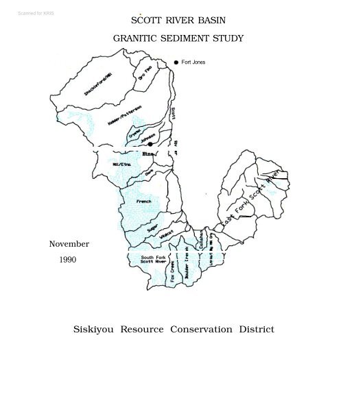
<strong>SCOTT</strong> <strong>RIVER</strong> <strong>BASIN</strong><br />
<strong>GRANITIC</strong> <strong>SEDIMENT</strong> <strong>STUDY</strong><br />
South Fork (<br />
Fort Jones<br />
Siskiyou Resource Conservation District
<strong>SCOTT</strong> <strong>RIVER</strong> WATERSHED<br />
<strong>GRANITIC</strong> <strong>SEDIMENT</strong> <strong>STUDY</strong><br />
by<br />
Sari Sommarstrom, Ph.D.<br />
and<br />
Elizabeth Kellogg<br />
Jim Kellogg<br />
of<br />
Tierra Data Systems<br />
for the<br />
SISKIYOU RESOURCE CONSERVATION DISTRICT<br />
Funding Provided by the<br />
Klamath River Basin Fisheries Task Force<br />
U.S. Fish and Wildlife Service<br />
Cooperative Agreement 14-16-001-89506<br />
November, 1990
ACKNOWLEDGEMENTS<br />
Many people gave generously of their time in helping the<br />
authors gather the data and develop the interpretations necessary<br />
for this report. Certain individuals also reviewed the draft<br />
report and offered useful suggestions (*). Sincere appreciation is<br />
extended to the following people:<br />
California Dept. of Fish and Game<br />
Dennis Maria, Ron Dotson, Jim Hopelain, Phil Baker*<br />
California Dept. of Forestrv<br />
Bob Williams, Virginia Whistler<br />
California Dept. of Transportation<br />
Al Trujillo<br />
California Dent. of Water Resources<br />
Koll Buer*, Doug Denton, Charles Ferchaud, Clyde Muir<br />
Fruit Growers Supply Company<br />
Richard Dragseth, Charles Brown<br />
North Coast Resional Water Quality Control Board<br />
Bob Klamt*<br />
Redwood National Park<br />
Danny Hagan, Bill Weaver<br />
Sierra Pacific<br />
Scott Warner<br />
U.S. Bureau of Land Management<br />
Bob Simmons<br />
U.S. Fish and Wildlife Service<br />
Ron Iverson*, Bill Brock*, Mike Stempel<br />
U.S. Forest Service<br />
Juan delaFuente*, Bernie Halterman, Tom Laurent*, Jim<br />
McGinnis, Scott Miles, Jay Power*, Dr. Leslie Reid*, Rick<br />
Svilich, Roberta Van de Water*, John Veevaert*, Jack West*<br />
U.S. Soil Conservation Service<br />
Bob Bartholomew, Joe Jahnke, Alvin Lewis, Dave Patterson*,<br />
Jan Dybdal, Nick Pappas*, Lyle Steffen*<br />
Individuals<br />
Dr. Howard Chang, Hydraulic Engineer, San Diego State Univ.<br />
Millard Coots, retired, Calif. Dept. of Fish and Game<br />
Frank Jackson, retired, Soil Conservation Service, Etna<br />
Chuck and Jim Jopson, pilots<br />
Orel Lewis, retired County Roads Commissioner and surveyor<br />
Bernita Tickner, Siskiyou County - Etna Branch Librarian<br />
Landowners along the Scott River who granted access
TABLE OF CONTENTS<br />
Page<br />
CREDITS ................................................... i<br />
ACKNOWLEDGEMENTS.......................................... ii<br />
TABLE OF CONTENTS......................................... iii<br />
ABSTRACT.................................................. viii<br />
Chapter 1. INTRODUCTION<br />
Purpose .............................................. l-l<br />
Sediment Budgets..................................... l-l<br />
Study Area........................................... l-2<br />
Precipitation ................................... l-2<br />
Runoff .......................................... l-2<br />
Topography ...................................... l-2<br />
Geology and Soils ............................... l-4<br />
Vegetation...................................... l-4<br />
Resource History..................................... l-4<br />
Early History................................... l-4<br />
Mining History.................................. l-5<br />
Timber Harvest History.......................... l-7<br />
Fire History.................................... l-7<br />
Stream Channel Modifications.................... l-8<br />
Water Use History............................... l-8<br />
References ........................................... l-9<br />
Chapter 2. UPLAND <strong>SEDIMENT</strong> SOURCES<br />
Introduction ......................................... 2-l<br />
Components of the Natural System that Impact<br />
Erosion Rates................................. 2-l<br />
Weather .................................... 2-l<br />
Topography and Hydrology................... 2-2<br />
Soils ..................................... 2-6<br />
Geology and Hydrology...................... 2-9<br />
Vegetative Cover and Effect of Land Use .... 2-11<br />
Methods.............................................. 2-16<br />
Approach Selected and Definitions............... 2-16<br />
Procedure for Roads and Skid Trails ............. 2-17<br />
Procedure for Streambanks....................... 2-20<br />
Procedures for Hillslopes, Timber Harvest Units,<br />
and Landslides............................. 2-22<br />
Sediment Yield Estimates........................ 2-26<br />
Results and Discussion............................... 2-31<br />
Roads ........................................... 2-31<br />
Skid Trails..................................... 2-33<br />
Streambanks ..................................... 2-33<br />
Sheet and Rill Erosion.......................... 2-34<br />
Soil Loss Summary............................... 2-35<br />
Sediment Storage and Yield...................... 2-39<br />
Accelerated vs. Natural Erosion and Yield ....... 2-42<br />
Grain Size Distribution......................... 2-42<br />
Needs for Further Study ......................... 2-43
References. . . . . . . . . . . . . . . . . . . . . . . . . . . . . . . . . . . . . . . . . . .<br />
Page<br />
2-45<br />
Chapter 3. <strong>SEDIMENT</strong> STORAGE AND TRANSPORT IN THE <strong>SCOTT</strong> <strong>RIVER</strong><br />
Introduction ......................................... 3-1<br />
Background........................................... 3-2<br />
Valley Geology.................................. 3-2<br />
Hydrology....................................... 3-3<br />
History of Channel Alterations .................. 3-3<br />
Commercial Sand and Gravel Extraction........... 3-9<br />
Methods.............................................. 3-9<br />
Existing Data................................... 3-9<br />
New Field Work.................................. 3-10<br />
Sediment Storage................................ 3-14<br />
Sediment Transport.............................. 3-15<br />
Results and Discussion............................... 3-17<br />
Stream Profile and Cross-Sections ............... 3-17<br />
Grain Size Composition.......................... 3-21<br />
Sediment Storage................................ 3-22<br />
Sediment Transport.............................. 3-28<br />
Comparison of Formulas ..................... 3-28<br />
Comparison of Reaches...................... 3-31<br />
Transport Processes........................ 3-32<br />
Analysis of Storage and Transport Data .......... 3-34<br />
Implications for the Future..................... 3-35<br />
Further Studies................................. 3-36<br />
References........................................... 3-37<br />
Chapter 4. IMPACTS ON SALMONID SPAWNING GRAVELS<br />
Introduction ........................................<br />
Effects of Sand and other Fine Sediments ........<br />
History of Scott River's Habitat Quality ........<br />
Stream Habitat Quality.....................<br />
Salmon and Steelhead Population............<br />
Extent of Spawning Habitat.................<br />
Methods..............................................<br />
Locations .......................................<br />
Quantitative Methods............................<br />
Transects ..................................<br />
Collection of Samples......................<br />
Analysis of Samples........................<br />
Sample Size................................<br />
Quality Indices.................................<br />
Percentage of Fines ........................<br />
Geometric Mean Diameter....................<br />
Fredle Index...............................<br />
Statistics ......................................<br />
Qualitative Methods.............................<br />
Results and Discussion...............................<br />
Sediment Size Composition.......................<br />
Statistical Evaluation..........................<br />
Quality Indices.................................<br />
Percentage Fines ...........................<br />
Historic Trends.......................<br />
4-l<br />
4-l<br />
4-3<br />
4-3<br />
4-6<br />
4-9<br />
4-9<br />
4-9<br />
4-12<br />
4-12<br />
4-12<br />
4-12<br />
4-13<br />
4-13<br />
4-13<br />
4-14<br />
4-14<br />
4-15<br />
4-15<br />
4-16<br />
4-16<br />
4-16<br />
4-17<br />
4-17<br />
4-25
Geometric Mean Diameter.................... 4-26<br />
Fredle Index............................... 4-30<br />
Visual Analysis............................ 4-32<br />
Conclusions .......................................... 4-35<br />
Use of Quality Indices .......................... 4-35<br />
Comparison of Sites............................. 4-36<br />
References........................................... 4-42<br />
Chapter 5. SUMMARY AND CONCLUSIONS<br />
Chapter 2 ............................................<br />
Chapter 3 ............................................<br />
Chapter 4 ............................................<br />
5-2<br />
5-5<br />
5-6<br />
APPENDICES<br />
A. Sediment Transport Capacity Formulas.............. A-l<br />
B. Scott River Cross-Sections ........................ B-l<br />
c. Spawning Area Grain Size Distributions ............ C-l<br />
D. Summary of Project Expenditures ................... D-l<br />
Figure<br />
LIST OF FIGURES<br />
l-l Study Area...................................... l-3<br />
l-2 Historic Map of Scott Valley, 1852 .............. l-6<br />
2-l<br />
2-2<br />
2-3<br />
2-4<br />
2-5<br />
2-6<br />
2-7<br />
2-8<br />
2-9<br />
2-10<br />
2-11<br />
Scott River Watershed Hydrology .................<br />
Scott River Watershed Granitic Geology/Soils ....<br />
Scott River Watershed Land Ownership............<br />
Scott River Watershed Roads and Skid Trails .....<br />
Scott River Watershed Earth Flows/Landslides ....<br />
Scott River Watershed Timber Harvest History....<br />
Photographs of eroded slopes, cut banks and<br />
skid trails in Study Area ..................<br />
Photographs of streambank scour, cut bank, and<br />
landslides in Study Area ...................<br />
Pie chart of annual erosion amounts by type .....<br />
Pie chart of annual erosion percentages by<br />
sub-basin ..................................<br />
Granitic sediment sources, storage and yield ....<br />
Paae<br />
2-5<br />
2-8<br />
2-15<br />
2-21<br />
2-23<br />
2-27<br />
2-29<br />
2-30<br />
2-38<br />
2-38<br />
2-44<br />
3-l Scott River - Mean monthy discharge ............. 3-4<br />
3-2 Scott River - Total discharge................... 3-5<br />
3-3 Scott River - Maximum daily discharge ........... 3-6<br />
3-4 Lower Scott River, early 1950s.................. 3-8<br />
3-5 Scott Valley watershed, reach location map ...... 3-12<br />
3-6 Stream profile, from mouth to headwaters ........ 3-18<br />
3-7 Scott River stream profile, study area .......... 3-19<br />
3-8 River classification............................ 3-20<br />
3-9 Scott River sediment and sand storage........... 3-24<br />
3-10 Scott River, Hwy.3 bridge cross-section......... 3-25<br />
3-11 Photo, Silt and debris after Dec. 1955 flood .... 3-26<br />
3-12 Photo, Reach 2 after Dec. 1964 flood ............ 3-26<br />
3-13 Changes in bed elevation at USGS Gage ........... 3-27
3-14 Scott River sediment transport capacity......... 3-33<br />
4-1<br />
4-2<br />
4-3<br />
4-5<br />
4-6<br />
4-7<br />
4-8<br />
4-9A<br />
4-9B<br />
4-10<br />
4-11<br />
4-12<br />
4-13<br />
4-14<br />
4-15<br />
4-16<br />
Table<br />
2-l<br />
2-2<br />
2-3<br />
2-4<br />
2-5<br />
2-6<br />
2-7<br />
2-8<br />
2-9<br />
2-10<br />
2-11<br />
2-12<br />
2-13<br />
2-14<br />
2-15<br />
2-16<br />
Water percolation through spawning gravel.......<br />
King salmon aerial spawning survey, Oct. 1962...<br />
Fall chinook spawners in Scott River, 1978-1989.<br />
Locations of sampling sites.....................<br />
Percent Fines - Scott River.....................<br />
Regressions of survival against Percent Fines...<br />
Relationship between fines and survival to<br />
emergence . . . . . . . . . . . . . . . . . . . . . . . . . . . . . . . . . .<br />
Upper and lower confidence intervals for steelhead<br />
fry emergence and percent fines.......<br />
Upper and lower confidence intervals for<br />
chinook salmon fry emergence...............<br />
Paae<br />
4-2<br />
4-5<br />
4-8<br />
4-11<br />
4-20<br />
4-22<br />
4-22<br />
4-23<br />
4-23<br />
Geometric mean - Scott River....................<br />
Relationship between percent embryo survival and<br />
substrate composition (dg) .................<br />
Relationship between dg and survival ............<br />
Fredle index - Scott River ......................<br />
Survival to emergence in relation to fredle (f).<br />
Visual Substrate Score..........................<br />
Spawning gravel quality in Scott Valley.........<br />
4-28<br />
4-29<br />
4-29<br />
4-31<br />
4-31<br />
4-33<br />
4-40<br />
LIST OF TABLES<br />
Major subwatersheds of western Scott River<br />
watershed with granitic soils..............<br />
Descriptive summary of watershed drainage<br />
patterns . . . . . . . . . . . . . . . . . . . . . . . . . . . . . . . . . . .<br />
Granitic soil types, erosion hazard ratings, and<br />
acreages . . . . . . . . . . . . . . . . . . . . . . . . . . . . . . . . . . .<br />
Total acres harvested on DG soils by watershed<br />
and ownership . . . . . . . . . . . . . . . . . . . . . . . . . . . . . .<br />
Road cut and fill lateral recession rate<br />
categories and descriptions................<br />
Road mileage, area, and density by watershed....<br />
Skid Trail mileage, area and density on DG......<br />
Road erosion sampling summary, 1989.............<br />
Miles of streams affected by scour . . . . . . . . . . . . .<br />
Average annual sheet and rill erosion on DG<br />
under natural and current harvest patterns.<br />
Summary of estimated soil loss by watershed and<br />
by source . . . . . . . . . . . . . . . . . . . . . . . . . . . . . . . . . .<br />
Percent of soil loss contributed by various<br />
sources for each sub-basin.................<br />
Sediment yield estimates using various delivery<br />
ratios and PSIAC method....................<br />
PSIAC sediment yield results by watershed.......<br />
Estimate of granitic sediment yield for Scott<br />
River sub-basins compared to other areas...<br />
Grain sizes of 58 sediment samples..............<br />
2-4<br />
2-4<br />
2-7<br />
2-14<br />
2-18<br />
2-19<br />
2-20<br />
2-31<br />
2-34<br />
2-35<br />
2-36<br />
2-37<br />
2-40<br />
2-41<br />
2-42<br />
2-43
3-l Scott River reach descriptions .................. 3-11<br />
3-2 Grain size classification....................... 3-13<br />
3-3 Comparison of sediment transport equations ...... 3-16<br />
3-4 Grain size composition by reach ................. 3-21<br />
3-5 Estimated volume of stored sediment by reach .... 3-23<br />
3-6 Average annual sediment transport capacity ...... 3-29<br />
3-7 Sensitivity analysis of transport equations ..... 3-30<br />
4-l<br />
4-2<br />
4-3<br />
4-4A<br />
4-4B<br />
4-5<br />
4-6<br />
4-7<br />
4-8<br />
4-9<br />
4-10<br />
4-11<br />
4-12<br />
Summary of Scott River Chinook salmon carcass<br />
recovery, 1979-1989 . . . . . . . . . . . . . . . . . . . . . . . .<br />
Locations of substrate sampling.................<br />
Substrate Characteristics and Associated Ranks<br />
for Calculation of Substrate Scores........<br />
Sediment Composition by Percentage..............<br />
Cumulative Percentage of Fine Sediments.........<br />
Predicted rates of emergence by percentage fines<br />
Historic comparison of percent fines with<br />
tributary sites, 1982 vs. 1989.............<br />
Geometric mean diameter and estimated survival..<br />
Fredle Index (f) results and estimated survival.<br />
Visual Surface Analysis - Substrate Score.......<br />
Summary of Index Mean Values....................<br />
Statistically Comparable Sites..................<br />
Ranking of Sites by Index.......................<br />
4-7<br />
4-10<br />
4-16<br />
4-18<br />
4-19<br />
4-24<br />
4-25<br />
4-27<br />
4-30<br />
4-34<br />
4-37<br />
4-38<br />
4-39
Sari<br />
<strong>SCOTT</strong> <strong>RIVER</strong> <strong>BASIN</strong> <strong>GRANITIC</strong> <strong>SEDIMENT</strong> <strong>STUDY</strong><br />
by<br />
Sommarstrom, Elizabeth Kellogg and Jim Kellogg<br />
Consultants<br />
for the<br />
Siskiyou Resource Conservation District<br />
Etna, California<br />
ABSTRACT<br />
The extent of the decomposed granitic (DG) sediment problem<br />
is examined in the Scott River watershed of Siskiyou County,<br />
California. This sand-sized sediment was previously identified to<br />
cause spawning habitat impacts for salmon and steelhead and to be<br />
an important factor constraining anadromous fish production in the<br />
Scott River, a large tributary of the Klamath River. Data was<br />
collected during 1989-90 within the 215,500 acre Study Area,<br />
which also included the Scott Valley portion of the Scott River<br />
and several tributaries. Analysis focuses on three aspects of the<br />
problem: (1) sources of granitic sediment production; (2) granitic<br />
sediment storage and transport in the Scott River; and (3) extent<br />
of impact of granitic sediment on salmon and steelhead spawning<br />
habitat in the Scott River and selected tributaries.<br />
To help analyze the large quantity of data, a Geographic<br />
Information System (GIS) database was developed of the Study Area,<br />
of which 57,000 acres (26%) are granitic soils. Soils developed<br />
from granitics are recognized as some of the most erodible. Total<br />
upland decomposed granitic erosion is estimated to be about<br />
340,450 tons per year. Road cuts constitute 40% of the amount,<br />
streambanks 23% road fills 21%, skid trails 13%, and the balance<br />
from road surfaces, other sheet and rill erosion, and landslides.<br />
For most years, sediment production in the Study Area is stored in<br />
the upper watershed. A delivery ratio of 0.21 is preferred for<br />
estimating annual sediment yield to the Scott River, based on<br />
results of a recent reservoir study in a similar area. An average<br />
yield of 71,500 tons of decomposed granitic sediment is therefore<br />
predicted to be delivered to the Scott River each year.<br />
Although the low gradient reaches of the river in Scott<br />
Valley represent a natural area of sediment deposition,<br />
considerable channel alteration of the Scott River over the years<br />
has changed its sediment storage and transport capacities. The<br />
greatest amount of sand in channel storage is in the reach between<br />
Oro Fino Creek and the State Highway 3 bridge near Fort Jones.<br />
Portions of this reach were affected by a diversion dam which<br />
acted as a sediment trap from 1958 until its removal in 1987-89.<br />
Adjustments in slope and transport capacity will continue to occur<br />
1
oth upstream and downstream until a new equilibrium is<br />
established. Sediment transport equations, while very limited in<br />
accuracy, were useful in identifying relative sediment transport<br />
between reaches and possible contributing factors. The Engelund-<br />
Hansen and Ackers-White transport equations appeared the most<br />
comparable to actual stream conditions. Prevention and<br />
rehabilitation of DG erosion in the uplands of the Scott River<br />
watershed would serve to decrease the input side of the local<br />
sediment budget and allow more of the DG sand in channel storage<br />
to get moved out over the long term.<br />
Existing and potential spawning areas were sampled for grain<br />
size composition using 238 McNeil sampler cores at 11 sites in the<br />
Scott River, and 55 cores at 6 sites in lower Etna, French and<br />
Sugar Creeks. Core samples were sieved into 7 size categories for<br />
analysis. Four quality indices were applied to the field data:<br />
percentage fines, geometric mean, fredle index, and visual<br />
substrate score. For percentage fines less than 6.3 mm, the three<br />
worst sites had amounts ranging from 82.1% to 92.7%, amounts which<br />
were greater than any reported in the literature. The relative<br />
ratings of the various indices for each site are quite consistent<br />
except for the fredle index. Quality indices best serve as<br />
relative measurements between sites and between years rather than<br />
as accurate predictors of emergent survival. The spawning gravel<br />
data developed for this study serves as a good baseline for<br />
monitoring changes in streambed composition of the Scott River and<br />
several tributaries.<br />
2
CHAPTER 1<br />
INTRODUCTION<br />
Purpose<br />
The 1985 Klamath River Basin Fisheries Resource Plan<br />
(CH2M-Hill, 1985) identified "spawning habitat sedimentation" as<br />
the second most important factor constraining anadromous fish<br />
production in the Scott Subbasin. Findings in the plan noted that<br />
decomposed granitic soils (commonly referred to as " DG") are the<br />
main source of sediment. This study was designed to better<br />
characterize the extent of the DG problem.<br />
Each of the three following objectives is the focus of<br />
successive chapters.<br />
Objectives<br />
A. Analyze watershed dynamics and determine sources of<br />
granitic sediment production in the Scott River Basin<br />
(Chapter 2).<br />
B. Determine granitic sediment storage and transport in the<br />
Scott River, within Scott Valley (Chapter 3).<br />
c. Determine the impact of granitic sediment on salmon and<br />
steelhead spawning in the Scott River and selected<br />
tributaries (Chapter 4).<br />
Each of the chapters provides new data collected during the past<br />
two years, and an analysis of the problem based on the new data.<br />
In addition, each chapter provides direction for concentrating<br />
further studies and restoration efforts.<br />
Sediment Budgets<br />
A sediment budget is the quantitative description of the<br />
movement of sediment through the landscape. To be complete, it<br />
considers the input rate or sediment production from hillslopes<br />
into the stream channels, the storage volume, and discharge rate<br />
of sediment (Swanson et al, 1982). A parallel can be seen between<br />
these elements of a sediment budget and the first two objectives<br />
of this study, which is a preliminary effort to provide some of<br />
the necessary data and analysis for a sediment budget of the Scott<br />
River. However, this study is focusing only on the decomposed<br />
granitic sediment portion of such a budget. It is also beyond the<br />
scope of the present effort to measure the actual discharge rate<br />
of sediment in the Scott River.<br />
Sediment budgets are useful in providing a measure of the<br />
relative importance of both natural and human-induced sediment<br />
sources. By identifying the major sediment sources, corrective<br />
measures can be applied to the "most beneficial points in the<br />
system" (Swanson et al, 1982).<br />
1-1
Study Area<br />
The Scott River Basin is located in south-central Siskiyou<br />
County, California, about 30 miles south of the Oregon border. The<br />
focus of this study is on the areas of the Scott River Basin that<br />
may produce decomposed granitic soils as well as the primary areas<br />
of sand deposition in the Scott River. Figure l-l represents this<br />
region of the watershed, which is located in the western,<br />
southwestern and southeastern portions of the Basin. The total<br />
area on the map is about 215,500 acres while the granitic soil<br />
types (mottled area) encompasses about 57,000 acres (26%).<br />
The sub-basins located within the study area are also<br />
indicated on the map. While other subbasins, such as Moffett<br />
Creek, may also contribute sediment, they are not sources of<br />
decomposed granitic sand and were therefore not included in the<br />
Study Area.<br />
The Study<br />
Basin (520,320<br />
Precipitation<br />
Area represents about 42% of the entire Scott River<br />
acres).<br />
The official Weather Bureau Station for the Scott Valley area<br />
is the U.S. Forest Service Ranger District Office in Fort Jones.<br />
A summary of the data (for the calendar year) follows:<br />
Station Elevation Period of Mean Season Minimum<br />
(feet) Record (inches) Maximum<br />
Fort Jones 2,747 1936-89 22.08 1949 10.05<br />
1970 35.07<br />
Two other precipitation stations, located in Etna and in Callahan<br />
(USFS Fire Station), have also collected rainfall data over the<br />
years.<br />
Precipitation data for the higher elevations have not been<br />
collected in the Study Area. Estimates, however, are available<br />
from an isohyetal map by Rantz (1968), which indicates 50 inches<br />
for the upper watershed boundary. Snowfall is common at elevations<br />
above 4000 feet throughout much of the winter (November to March).<br />
Runoff<br />
The Scott River is a principal tributary of the Klamath<br />
River. Annual discharge at the U.S.G.S. gage station below the<br />
Scott Valley averages 489,800 acre-feet. Runoff characteristics<br />
are described in detail in Chapter 3.<br />
Topography<br />
The Salmon Mountains encompass the western portion of the<br />
1-2
LOCATION MAP<br />
Figure 1-1<br />
Study Area<br />
1-3
study area, while the Scott Mountains border the south boundary<br />
and the Scott Bar Mountains border the north. The slope of the<br />
area varies from less than 2 percent in Scott Valley to over 60<br />
percent in the mountains. Elevation ranges from 2,620 feet at the<br />
Scott River at the north end of the valley to over 8,000 feet at<br />
several mountain peaks in the southwest.<br />
Geology and Soils<br />
Located within the eastern portion of the Klamath Mountains,<br />
the area's bedrock consists of metasedimentary and metavolcanic<br />
rocks of Late Jurassic and possibly Early Cretaceous Age. The<br />
alluvial fill in the valley contains unconsolidated Pleistocene<br />
and Recent deposits . An extensive area of granodioritic rock,<br />
intrusive into schists and greenstone, is exposed for about 8<br />
miles in the mountains paralleling the west side of Scott Valley.<br />
Every gradation between granite and quartz diorite occurs<br />
here. In the frequent shear zones, the granodiorite is "extremely<br />
friable and crumbles to the touch" (Mack, 1958).<br />
The granodiorite is the light-colored, coarse parent material<br />
for several DG soil types of varying depths and textures. Soils<br />
derived from granitics are noncohesive and usually highly erodible<br />
(Laake, 1979). Geology and soils are also discussed in Chapters 2<br />
and 3.<br />
Vegetation<br />
Most of the 100 square miles of valley land are under<br />
cultivation, primarily in alfalfa, grain and pasture. Riparian<br />
shrubs and trees line some portions of the stream system. In the<br />
foothills, oaks, junipers, shrubs and grasses predominate,<br />
particularly on the drier east side. Mixed conifers (mainly<br />
douglas fir, ponderosa pine, sugar pine and incense cedar) cover<br />
the upper western and southern watershed. Native hardwoods and<br />
understory shrubs are also scattered throughout the forest area<br />
(USSCS, 1972).<br />
Resource History of Scott Valley Watershed<br />
What is seen today in the Scott Valley watershed is quite<br />
different from 150 years ago. As found in other areas, certain<br />
postsettlement changes likely to have had major impacts on the<br />
nature of stream systems include beaver removal, mining,<br />
deforestation, urbanization, tillage, irrigation, channel<br />
alteration, grazing by domestic animals, and fire suppression.<br />
Identifying the changes that have occurred to the Scott River's<br />
landscape over the years of human activity is important to an<br />
understanding of what is happening today.<br />
Early History: Indians and Trappers<br />
The Shasta Tribe (Iruaitsu people) originally occupied the<br />
Scott Valley as part of their ancestral territory, sustaining<br />
1-4
themselves on acorns, deer and salmon. What impact their<br />
practices, such as burning, had on the presettlement conditions of<br />
the watershed is not known.<br />
In the 1830's the Hudson Bay trappers discovered "Beaver<br />
Valley"m and the "Beaver River? They reportedly trapped 1800<br />
beaver on both forks of the Scott River in one month. It was "the<br />
richest place for beaver I ever saw", claimed one trapper many<br />
years later. He also described the Scott Valley as all one swamp<br />
caused by the beaver dams. (Wells, 1881)<br />
While not all of the beaver were taken, this major removal<br />
likely had a significant effect on the Scott River and its<br />
tributaries. Beaver dams slow the movement of water, sediment, and<br />
streamside vegetation out of watersheds . As a result, more water<br />
is stored, the ground water is recharged, and more diverse<br />
vegetation grows along streams. Beaver ponds are also known to<br />
provide excellent habitat for young coho salmon (J. Sedell, in<br />
Bergstrom, 1985).<br />
In 1853, the earliest map of the "Scott's Valley" indicates<br />
that beaver dams were still obvious around Kidder Creek near<br />
Greenview (Figure l-2). The map also shows a defined stream<br />
channel for the Scott River rather than a marshy area of illdefined<br />
channels. In May 1855, one observer described the Scott<br />
River in the valley as "from thirty to forty yards in width, deep<br />
in many places, with a current of from five to seven miles per<br />
hour" (Metlar, 1856).<br />
Mining History<br />
Gold miners rediscovered the Scott River in 1851, beginning<br />
the settlement of the region. Within the study area, gold mining<br />
was most extensive in the South Fork of the Scott River and Oro<br />
Fino and Shackleford creeks, with lesser activity in French Creek<br />
and the East Fork. By 1856, hydraulic mining operations had made<br />
the lower Scott River near Scott Bar almost constantly "turbulent<br />
and muddy" while the Klamath River was usually "clear and<br />
transparent" (Metlar, 1856). To supply the miners over in the<br />
Salmon River country, a trail along Etna Creek going over Etna<br />
Summit was built, cutting into some DG soils. (This trail was<br />
gradually widened and eventually became a paved county road.)<br />
Floods in 1852-53, 1861, 1864, 1875, and 1880 "swept the<br />
rivers clear of all mining improvements" (Wells, 1881). In normal<br />
times, streams near placer mines were diverted into mining ditches<br />
of various capacities and lengths. Some of these ditches are still<br />
in operation (though mainly for irrigation) in the South Fork,<br />
East Fork, French Creek, Sugar Creek, and Etna Creek drainages.<br />
During the period from 1934 to about 1950, large gold dredges<br />
operated on the upper Scott River and Wildcat Creek. The largest<br />
Yuba dredge excavated to a depth of 50-60 feet below water line<br />
and processed millions of cubic yards of soil and gravel. In its<br />
wake were left tailings piles with large cobbles on top, lining<br />
1-5
I<br />
. .<br />
t . * i<br />
-- 7_- -Ti<br />
_ /At, - ----- -- ____ 5
the Scott River for about 5 miles below Callahan.<br />
Timber Harvest History<br />
Timber was originally needed for mining as well as for<br />
building purposes . Several sawmills were built in Scott Valley in<br />
1852 and 1860, with 11 mills sawing 3.5 million board feet per<br />
year by 1880. These mills were primarily located in Fort Jones,<br />
Etna, French Creek, and Kidder Creek (Wells, 1881).<br />
One of the first major roads into the "DG country" was built<br />
in 1933-34 by the California Conservation Corps, extending north<br />
to south across the upper French, Sugar, and Wildcat Creek<br />
drainages and ending up in the South Fork sub-basin. Today this<br />
unsurfaced road is referred by most as the "High C " or "C's" road.<br />
This access road provided the first opportunity for logging the<br />
higher elevations, which were still not entered until the late<br />
1950s according to U.S. Forest Service records.<br />
Logging began more intensively after World War II. In the<br />
1950s, Scott Valley's sawmill industry provided a substantial<br />
source of local income, with four mills cutting 40,000 or more<br />
board feet per day, and about 9 mills cutting 5,000 or more board<br />
feet per day (Mack, 1958). Timber harvest history data is<br />
presented and discussed in Chapter 2.<br />
Fire History<br />
Very little information about fire history is available.<br />
Although lightening-caused fires are fairly frequent in the<br />
mountains, extensive fires are not common in the study area<br />
as little volatile brush is present on the west side of the Scott<br />
Valley.<br />
The local California Dept. of Forestry office does not map<br />
past fires or keep any historical records. The only available data<br />
comes from a retired fire control officer from the Klamath<br />
National Forest, who personally recorded and published a fire<br />
history of Siskiyou County (Morford, 1984). A large map indicating<br />
the year of the largest fires was also prepared and can be seen at<br />
the County Museum in Yreka. From his book comes the following list<br />
of large fires in the study area of Scott Valley:<br />
Year Location (Township/Range/Section) Acres<br />
Burned<br />
1955 Kidder Creek - 42N/lOW:7 14,562<br />
1954 Sugar Creek - 40N/9W:ll 466<br />
1940 Etna Creek - 42N/9W:22 (41N?) 260<br />
1924 Crystal Creek - 42N/9W:5 8,900<br />
Etna Creek - 42N/lOW:32 160<br />
Kidder Creek - 42N/lOW:15,22 600<br />
l-7
By far the largest fire of record was the 1955 Kidder Creek<br />
fire, which occurred only a few months before the disastrous<br />
December 1955 flood. Adjacent portions of the Patterson Creek<br />
drainage were also burned at that time. The massive fires of 1987<br />
did not burn any significant acreage in the upper Scott River<br />
watershed.<br />
Stream Channel Modifications<br />
In addition to the beavers and mining, other human activities<br />
have altered the original stream channel shape, size and location.<br />
Chapter 3 provides an extensive discussion of stream channel<br />
changes.<br />
Water Use History<br />
Hay cutting and cattle grazing began in 1851 in Scott Valley<br />
to support the miners (Wells, 1881). Stream diversions to irrigate<br />
pastures and crops also began early. Pumping of ground water now<br />
supplements surface water sources. Water rights to Scott River<br />
surface water were adjudicated by the State of California in 1980.<br />
In 1988, the estimated agricultural water demand in the Scott<br />
Valley was about 96,400 acre-feet on 34,100 irrigated acres (C.<br />
Ferchaud, CDWR, pers. comm.).<br />
1-8
REFERENCES - CHAPTER 1<br />
Bergstrom, D. 1985. Beavers: biologists "rediscover" a natural<br />
resource. Forestry Research West, Oct. 1985: 1-5.<br />
CH2M-Hill. 1985. Klamath River Basin Fisheries Resource Plan.<br />
USDI, Bureau of Indian Affairs. Redding.<br />
Laake, R.J. 1979. California forest soils - a guide for<br />
professional foresters and resource managers and planners.<br />
Univ. Calif. Div. Ag. Sci., Publ. 4094. Berkeley, 180 p.<br />
Mack, S. 1958. Geology and ground-water features of Scott Valley,<br />
Siskiyou County, California. U.S. Geological Survey Water-<br />
Supply Paper 1462, Washington D.C., 95p.<br />
Morford, L. 1984. One hundred years of wildland fires in Siskiyou<br />
County. Privately published. Yreka, 124p.<br />
Rantz, S.E. 1967. Mean annual precipitation-runoff relations in<br />
North Coastal California, U.S. Geological Survey Prof. Paper<br />
575-D, pp. D281-D283.<br />
Swanson, F.J., R.J. Janda, T. Dunne, and D. Swanston. 1982.<br />
Sediment budgets in forested drainage basins. U.S. Forest<br />
Service, Gen. Tech. Report PNW-141, Portland. 165 p.<br />
U.S. Soil Conservation Service. 1972. Inventory and evaluation of<br />
the natural resources, Scott River Watershed, Siskiyou<br />
County, California. Siskiyou Resource Conservation District.<br />
Yreka, 73 p.<br />
Wells, H.L. 1881. History of Siskiyou County, California. D.J.<br />
Stewart & Co., Oakland (reprinted in 1971), 240p.<br />
Williams, R.S. 1852. Plot map of Scotts Valley. U.S. Army,<br />
Washington, D.C., lp.<br />
1-9
CHAPTER 2<br />
UPLAND <strong>SEDIMENT</strong> SOURCES<br />
Introduction<br />
Objective: To identify and estimate the relative importance of<br />
upland sources of granitic sediment affecting the<br />
Scott River within Scott Valley.<br />
A granitic watershed's response to land use activities is very<br />
different and sometimes unique compared to watersheds of other<br />
geologic types. Soils developed from granitics are recognized as<br />
some of the most erodible and natural erosion occurs continuously<br />
at a higher rate compared to most other soils (Anderson, 1976, for<br />
example).<br />
Because of the preliminary nature of this study the emphasis<br />
was kept to use of existing databases, aerial photoanalysis, and<br />
limited field activity to derive results. Results are reasonable<br />
estimates rather than statistically precise measures.<br />
Components of the Natural System That Impact Erosion Rates<br />
The following components of the natural environment control<br />
erosion rates in specific ways that are not always well understood.<br />
Weather<br />
Precipitation patterns. Precipitation averages are important<br />
in assessing erosion for the following reasons: 1) They reflect<br />
the potential for overland flow and runoff given equivalent slope<br />
conditions: 2) When viewed in relation to average temperatures,<br />
they represent the potential for natural cover on the landscape; 3)<br />
Despite the importance of episodic climatic events dominating the<br />
timing of sedimentation into stream channels, mean annual<br />
precipitation has been shown to be a relatively precise indicator<br />
of climatic stress on sedimentation in Northern California<br />
(Anderson, 1976); and 4) Precipitation averages tend to parallel<br />
rainfall intensities, which have a more direct impact on erosion<br />
rate.<br />
A measure of short duration precipitation intensity is the<br />
two-year, six-hour level of rainfall, which in our study area<br />
ranges from 0.95 inches at Ft. Jones (1944-1983 records, Dept. of<br />
Water Resources, 1986) to about 3.0 inches at the highest<br />
elevatio and McDonough, 1976).<br />
. The relative percentage of rain<br />
2-l
versus snow for different portions of the watershed affects erosion<br />
rates. Snow will be generally protective of the soil surface from<br />
rain, wind and dry ravel erosion, but rapid melting can increase<br />
erosion. Snowmelt can increase, decrease or delay peak flows<br />
(Harr, 1981; Harr and McCorison, 1979), depending on interacting<br />
climatic patterns, aspect, and antecedent watershed conditions. It<br />
can also affect how water is routed to stream channels.<br />
On south-<br />
facing slopes in forest openings, either natural or the result of<br />
timber harvest, the formation of density layers in the snowpack can<br />
cause delivery of water downslope into channels rather than<br />
vertically into the soil profile (Smith 1974, 1979).<br />
Forest openings affect the rate of snowmelt, hence the volume<br />
and pattern of peak flows. Sediment yields triggered by snowmelt<br />
from logging treads on granitic roads in the Idaho Batholith were<br />
less than yields triggered by rainfall by several orders of<br />
magnitude (Vincent, 1982).<br />
On the whole it is believed that snowpack at the higher<br />
elevations in our study area decreases the potential for erosion,<br />
except during rain-on-snow events which trigger large runoffs such<br />
as occurred during the 1964 flood. In a study by Anderson (1976),<br />
when rain-snow relationships are considered with using mean annual<br />
precipitation values in Northern California, an increase in<br />
precipitation by a factor of three produces only a 36 percent<br />
increase in reservoir deposition. Based on data from this same<br />
work, snow comprises about 17 percent of total precipitation at<br />
3500 ft. elevations at the latitude of our study area, 30 percent<br />
at 4500 ft., 48 percent at 5500 feet, and 68 percent at 6500 feet.<br />
Topography and Hydrology as They Impact Upslope Sedimentation<br />
Granitic landscapes are generally shaped by differential<br />
weathering, glaciation and surface processes such as shallow debris<br />
slides and dry creep (or ravel). Stream action, earthflows and<br />
slumps are typically less important than in other geologic types<br />
(Seidelman, 1984, Baldwin and de la Fuente, 1987). Landscape<br />
patterns such as slope steepness, aspect, elevation and drainage<br />
density differentially affect rates of sedimentation. These<br />
elements are discussed separately below.<br />
Slope. In equivalent climates, steep slopes can dominate<br />
erosion rates, as soil loss increases much more rapidly than runoff<br />
with slope. The angle of repose for granitic rock decreases as it<br />
decomposes (Durgin, 1977), and is determined to be about 35 degrees<br />
(70 percent) for DG soils (Lumb, 1962; Gray and Megahan, 1981).<br />
Studies have shown an increase in the occurrence of debris slides<br />
above this angle up to 42 degrees (90 percent) (Megahan, 1978).<br />
Steeper slopes tend to be bedrock and not prone to these<br />
superficial slides. Seidelman (1984) suggests that slopes over 30<br />
degrees (60 percent) be considered sensitive in weathered granitic<br />
2-2
terrain. Such slopes are often anchored by tree roots, so are<br />
quite vulnerable to timber harvest disturbance.<br />
Only about two percent of the slopes on DG in the Scott River<br />
watershed are mapped at gradients of between 60 and 90 percent (at<br />
a resolution of 1.6 acres). This does not include road cuts,<br />
cliffs, steep inner gorges and channel sides which are averaged<br />
with gentler slopes so do not show up at this elevation model<br />
resolution. In effect, there is considerably more area with 60 to<br />
90 percent slope than is found on the map.<br />
Aspect. Aspect plays a role in erosion rates. Prevailing<br />
winds during storms cause more precipitation to fall on south and<br />
west exposures. Runoff and erosion are higher due to more rainfall<br />
and less cover because these aspects also dry faster and have<br />
thinner soils. Warmer exposures are more affected by freeze-thaw<br />
cycles than cooler aspects, although amount of ground cover can<br />
complicate this pattern.<br />
Twenty-four percent of the DG area in the Scott River<br />
watershed faces between south and west.<br />
Elevation. DG soils at the upper elevations are more erodible<br />
because of coarse grain sizes more typical there. Physical<br />
weathering predominates at these elevations because of cooler<br />
temperatures, whereas chemical weathering, clay formation and flood<br />
flows are maximized at intermediate elevations so higher<br />
sedimentation rates occur there (Anderson, 1976). Higher<br />
elevations also have more snowpack protection, and more slope and<br />
streambed armoring by granitic boulders. Depth to bedrock also<br />
plays a role as debris slides are more common in granitic soil more<br />
than two feet deep (Wilson and Hicks, 1975). The mid-elevations<br />
are more eroded despite higher percentages of silt and clay and<br />
deeper soil development. This phenomenon is noticeable in the<br />
Study Area and has been documented by Colwell (1979) in the<br />
Sierras. The lower elevations (less than 3000 feet) have less<br />
erosion hazard due to lower rainfall and gentler slopes.<br />
Geomorphology (stable versus unstable landforms) can complicate<br />
elevation patterns of soil development (Tom Laurent, Klamath<br />
National Forest, pers. comm.).<br />
Drainaae pattern Table 2-l shows the major subwatersheds of<br />
the Study Area, their total area and proportion underlaid by<br />
granitic soils. Table 2-2 is a descriptive summary of drainage<br />
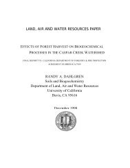
patterns by watershed. Figure 2-l depicts Study Area hydrology<br />
with watershed boundaries in black and the streams color-coded by<br />
their order. Streams were ordered based on those mapped on recent<br />
USGS 7-1/2' topographic quadrangles, using the stream order<br />
classification of Strahler (1957). The blue-line streams highest<br />
in the watershed were considered first order. We did not infer<br />
unmapped first-order streams as described by Goudie (1981).<br />
2-3
Table 2-1. Major subwatersheds of the western Scott River<br />
watershed, their total areas and proportions<br />
underlaid by granitic soils. The granitic Study Area<br />
is about 89 square miles.<br />
Total Granitic % of<br />
Area Terrain Watershed % of<br />
Watershed (Acres) (Acres) in DG all DG<br />
Shackleford/Mill 31869 2104 7 4<br />
Kidder/Patterson 39919 3311 8 6<br />
Crystal 2316 1886 81 3<br />
Johnson 4394 843 19 1<br />
Mill/Etna 17399 6495 37 11<br />
Clark 3247 1007 31 2<br />
French 20584 12984 63 23<br />
Sugar 8149 5929 73 10<br />
Wildcat 5074 1418 28 2<br />
South Fork 15115 6600 44 12<br />
Fox 4605 2857 62 5<br />
Boulder 7992 6552 82 12<br />
Little/Big Mill 5876 3138 53 6<br />
East Fork 46686 527 1 1<br />
"Callahan" 2307 1230 53 2<br />
TOTALS 215532 56881 26 100<br />
Table 2-2. Descriptive summary of watershed drainage patterns.<br />
Watershed<br />
Drainage<br />
Density<br />
Ai Aq. Mi!<br />
Shack leford/Mi l l 2.3<br />
Kidder/Patterson 2.5<br />
Crystal 1.7<br />
Johnson 2.9<br />
Mill/Etna l l 2.1<br />
Clark 2.5<br />
French 3.1<br />
Sugar 3.5<br />
Wi ldcat 3.2<br />
South Fork 2.4<br />
Fox 1.8<br />
Boulder 2.1<br />
Little/Big Mill 2.2<br />
East Fork 2.0<br />
‘Ca l ahan" 3,3.1l<br />
Entire Watershed -<br />
Length of<br />
Al l Streams<br />
(Mi les)<br />
116.0<br />
156.0<br />
6.1<br />
19.6<br />
56.6<br />
12.5<br />
100.0<br />
44. 0<br />
25.2<br />
57.6<br />
13.3<br />
26.1<br />
20.5<br />
144.0<br />
11.2<br />
809<br />
Length of<br />
Di tches<br />
(Mi les)<br />
16.6<br />
20.3<br />
5.4<br />
5.5<br />
Lt.7<br />
20.6<br />
15.7<br />
8.2<br />
10.7<br />
0.6<br />
0.7<br />
30.7<br />
2.8<br />
Length of<br />
DC Streams<br />
(Mi les)<br />
5..4<br />
8.7<br />
1.8<br />
1.7<br />
10.8<br />
1.3<br />
33.7<br />
14.0<br />
3.0<br />
19.2<br />
5.6<br />
13.6<br />
6.6<br />
1.4<br />
2.1<br />
2 - 4<br />
Gronit Ic Port ion of Uatershed<br />
Order 1 Order 2 Order 3<br />
Streams Streams Streams<br />
(Mi les) (Mi les) (Mi les)<br />
2.5<br />
5.2<br />
1.1<br />
1.0<br />
6.0<br />
1.3<br />
16.9<br />
6.4<br />
2.1<br />
9.1<br />
2.6<br />
7.0<br />
3.7<br />
0.8<br />
1.9<br />
1.4<br />
1.8<br />
0.7<br />
0.7<br />
2.5<br />
7.9<br />
1.6<br />
0.5<br />
3.6<br />
1.1<br />
3.3<br />
2.9<br />
0.6<br />
0.2<br />
1.5<br />
1.7<br />
0.4<br />
6.3<br />
2.0<br />
1.9<br />
1.5<br />
3.3<br />
29 19<br />
Order 4<br />
Streams<br />
(MI les)<br />
1.9<br />
0.2<br />
2.2<br />
1.1<br />
5<br />
Order 5<br />
Streams<br />
(Mi les)<br />
Length of<br />
Ditches<br />
(Mi les)<br />
2.4<br />
1.8<br />
0.4<br />
2.1<br />
0.4
Figure 2-1<br />
2-5<br />
<strong>SCOTT</strong> <strong>RIVER</strong> WATERSH<br />
HYDROLOGY<br />
--- - - First Order<br />
- Second Order<br />
___ Third Order<br />
- Fourth Order<br />
___ Ditches
The steep, narrow canyons that typically dissect the Study<br />
Area facilitate the movement of soil particles into the stream<br />
system. Silt-sized particles and organic debris are expected to<br />
move constantly through the system and come from throughout the<br />
watershed. Sand-sized and larger particles are washed from roads<br />
and other sources and stored as lag deposits in swales and loworder<br />
channels until the larger storms can flush the system. This<br />
process of colluvial sediment storage and periodic flushing is<br />
evident in the Scott River watershed; It has been identified<br />
elsewhere by others and noted as the source of episodic sediment<br />
pulses (Pillsbury, 1976; Dietrich and Dunne, 1978; Dietrich et al.,<br />
1982; Tsukamoto et al., 1982; Costa, 1984; Dietrich and Dorn, 1984;<br />
Rolle et al., 1987; and USDA-Forest Service, 1990).<br />
Also recognized by some workers in granitic terrain are high<br />
streambank erosion rates due partly to the erodibility of the<br />
coarse grain sizes and partly to the development of "stepped,"<br />
alluviated reaches in between areas of bedrock (Wahrhaftig, 1965;<br />
California Resources Agency, 1969; Seidelman, 1984). Transport<br />
capacity is reduced in the alluvial reaches. Low gradient,<br />
alluvial reaches vegetated with willows and alders are evident in<br />
larger Study Area watersheds below sites of serious, upper<br />
streambank erosion created by the 1964 flood, probably caused by<br />
debris torrents in the low-order, well-armored channels (see<br />
Pierson, 1977, for a discussion of debris torrents). These are<br />
clearly sites of long-term storage. Seidelman also believes<br />
aggradation in granitic streambeds to be temporary and localized,<br />
due to the predominance of sand-sized material that is relatively<br />
easily moved.<br />
Finally, Seidelman (1984) has observed the lack of interaction<br />
between soil disturbance, including inner gorge debris slides, and<br />
high stream flows in granitic terrain compared to other geologic<br />
types. He suggests that fish habitat and reservoir storage are<br />
reduced in direct proportion to volume of sediment deposited into<br />
streams (rather than a synergistic or cumulative relationship). He<br />
concludes that "it is likely that the most significant stream flow<br />
effect of soil disturbance is the interception of subsurface flow<br />
by roads incised into bedrock," instead of any effect on peak<br />
flows. This phenomenon associated with granitic roads is discussed<br />
more thoroughly later in this report.<br />
Soils<br />
Soils for the Study Area were mapped by the Soil Conservation<br />
Service on private land (USDA-SCS, 1983) and the U.S. Forest<br />
Service on public land (USDA-FS, 1982). The classification systems<br />
differ somewhat between the agencies, as can be seen in Table 2-3,<br />
where soil types, their erosion hazard ratings and acreages are<br />
listed. (The Forest Service classified soils to the family level,<br />
while the Soil Conservation Service used the series level.) The<br />
2-6
soil surveys' delineation of soils is different in some locations<br />
than that of granitic geology defined on the smaller scale, USGS<br />
Weed quadrangle geology map (1:250,000) (Wagner, 1987).<br />
Discrepancies are evident on the map, Figure 2-2.<br />
Table 2-3. Granitic soil types of the Study Area from the Soil<br />
Conservation Service and Forest Servoce surveys, their erosion<br />
hazard ratinas and acreages.<br />
Map<br />
Code Soil Type<br />
U.S.<br />
124<br />
127<br />
128<br />
130<br />
162<br />
165<br />
166<br />
189<br />
Forest Service survey:<br />
Entic Xerumbrepts-Gerle<br />
Gerle-Entic Xerumbrepts<br />
Gilligan-Chawanakee<br />
Gilligan-Holland<br />
Lithic Xerumbrepts-Rock<br />
Outcrop<br />
Nanny (glacial till)<br />
Nanny (glacial till)<br />
Teewinot-Endlich<br />
Percent<br />
Slope<br />
Erosion<br />
Hazard Acres<br />
30-90<br />
50-90<br />
30-90<br />
15-70<br />
high<br />
high<br />
high<br />
high<br />
3388<br />
11073<br />
3549<br />
8356<br />
15-90<br />
2-30<br />
30-50<br />
50-90<br />
high<br />
moderate<br />
moderate<br />
very high<br />
421<br />
5267<br />
6261<br />
11572<br />
U.S. Soil Conservation Service survey:<br />
119 Chaix-Chawanakee gravelly<br />
coarse sandy loam 5-30 mod.-high<br />
120 Chaix-Chawanakee gravelly<br />
coarse sandy loam 30-50 high<br />
121 Chaix-Chawanakee gravelly<br />
coarse sandy loam 50-70 very high<br />
693<br />
4222<br />
8280<br />
The parent material of these soil types ranges in composition<br />
from "hard granitic rock" to "soft, disintegrated decomposed<br />
granitic rock."/ Rock composition ranges from coarse-grained quartz<br />
monzonite to diorite. Soil depth typically ranges from less than<br />
10 inches on the Chawanakee and Teewinot, to more than 60 inches on<br />
glacial till or the more developed Holland type. Surface textures<br />
range from loam to very gravelly sandy loam, with most soils in the<br />
gravelly sandy loam category. The Chawanakee surface layer is less<br />
than four inches deep (one inch in the Forest Service survey).<br />
Subsoils have a greater range in texture depending on their<br />
development, from gravelly clay loams of Goldridge and Holland<br />
types, to the gravelly loamy sands of Nanny and Entic Xerumbrepts.<br />
The Teewinot soil lacks a subsoil. Chawanakee has the highest<br />
proportion of rock outcrop, typically about 25 percent of ground<br />
cover.<br />
2-7
<strong>SCOTT</strong> <strong>RIVER</strong> WATERSHED<br />
Geology<br />
Glacial deposits<br />
ILS
Geology and Hydrology<br />
Soils derived from granitics are widely agreed to be some of the<br />
most erodible of any rock type. In a northern California study<br />
based on surface aggregation ratio as a measure of erodibility,<br />
soils developed from acid igneous (granitic) rock were found to be<br />
two and one-half times more erodible than basalt (Andre and<br />
Anderson, 1961). They also produced three and one-half times more<br />
sediment to reservoirs than soils from other parent materials<br />
(Anderson, 1976).<br />
Importance of subsurface hydrology. The most important hydrologic<br />
process affecting erosion in DG soils is the subsurface, lateral<br />
flow of water at the saprolite-bedrock interface. When these flows<br />
are intercepted by forest roads the hydrology of the entire watershed<br />
can be affected. The road concentrates the water, diverting it<br />
onto fill slopes and from one stream channel to another. Overloaded<br />
channels will respond to the increased flows with what can be<br />
serious streambank erosion or downcutting, while fill slopes may<br />
gully or slough. Megahan (1972) believes this process increases<br />
total runoff volume from a watershed, but may not affect peak flows<br />
depending on how the excess is re-directed through the watershed.<br />
In his study, a single road located at the lower end of a watershed<br />
intercepted 35 percent of subsurface flows, resulting in runoff 7.3<br />
times the direct runoff from roads.<br />
Differences in stage of decomposition. An important characteristic<br />
of granitic soils is the stage of bedrock decomposition, as this<br />
affects the quantity and grain size of material available for<br />
transport. An entire spectrum of granitic weathering can occur<br />
among regions or even on the same slope. One area can have unweathered<br />
rock high on a slope to deep soils with well-developed,<br />
clay-rich subsoils on the sideslopes and toe (Durgin, 1977). Such<br />
progressions have been observed in the English Peak batholith of<br />
the Klamath Mountains (Rice et al. 1985) and is noteworthy in our<br />
Study Area with, for example, the Holland soil type when it occurs<br />
near slope toes, alluvial fans or stable landforms. Influencing the<br />
rate of parent rock decomposition are mineralogy, rock texture,<br />
porosity,fractures and joint structure. Of the four main minerals<br />
involved (quartz, biotite, plagioclase and orthoclase), biotite and<br />
plagioclase dominate the erosion process. Locally, the granodiorite<br />
is about 15 to 20 percent biotite and 60 percent sodic plagioclase<br />
(Mack, 1958). They expand by hydrolysis and oxidation, disintegrating<br />
into gruss and then sands, loamy sands or sandy loams. The<br />
quartz component remains unchanged except for disaggregation. This<br />
process occurs easiest when the minerals are in contact with soil<br />
water solutions in the zone of soil aeration (Ruxton and Berry,<br />
1957; Durgin, 1977).<br />
Within the soil profile, exposed portions of the granitic substrate<br />
that are wet only seasonally erode very slowly. Below this,<br />
typically, is a zone of weathered granite where chemical<br />
2-9
weathering predominates and more than 85 percent of the rock is<br />
weathered. Deeper is disintegrated granite where physical<br />
weathering predominates, then bedrock (Durgin, 1977; Rolle et al.<br />
1987). It is in the zone of chemical weathering in the soil<br />
profile and intermediate weathering with respect to the stage of<br />
decomposition (such gradations as can be seen on slopes or by<br />
elevation) where erosion activity is maximized.<br />
In general, differences in bedrock weathering are probably<br />
overshadowed by differences in precipitation pattern, slope<br />
steepness and internal soil drainage. This conclusion has been<br />
reached by Clayton et al. (1979) in the Idaho batholith and<br />
Seidelman (1984) for the Sierra Nevada.<br />
Surface processes. Under unburned, natural conditions,<br />
overland flow is not important compared to other erosive processes<br />
in DG terrain because of high permeability, good ground cover and<br />
the need for rapid, turbulent flow to carry the large grain sizes<br />
(Bloom, 1978). However, forest fires, road building and log<br />
skidding are activities that facilitate concentration of flows and<br />
currents in the sheetwash, hence of rills, gullies and ephemeral<br />
channels. Burned and other disturbed sites in the Scott River area<br />
frequently show evidence of turbulent, concentrated flow. However,<br />
the soil's non-cohesive grains tend to fall in on themselves (dry<br />
ravel) after some time, often erasing the tell-tale signs of these<br />
processes. Dry ravel or creep of loose particles can be an<br />
important surface process in DG soils. In an Idaho study (Megahan,<br />
1978), it was found to increase the rate of soil loss by an order<br />
of magnitude and constitute 15 percent of total loss. In the Study<br />
Area significant amounts of soil have been observed to be dislodged<br />
and moved off-slope by rainsplash on disturbed sites during even<br />
mild summer storms.<br />
Important to surface erosion processes in DG are organic<br />
matter and clay contents. Whereas clay acts as the primary binding<br />
agent in the soil, organic matter is more important in protecting<br />
the soil surface. Both are important to soil fertility and waterholding<br />
capacity. Both are selectively removed by surface erosion.<br />
For most soils, erodibility increases when organic matter<br />
decreases. For sandy soils, however, the opposite is true within<br />
the soil profile (Fink, 1970; Meeuwig, 1971). Components of the<br />
organic matter (fungal hyphae at high elevations (Tom Laurent,<br />
Klamath National Forest, pers. comm.)) coat the sand grains, making<br />
them hydrophobic and more easily disaggregated and moved off slope.<br />
This is thought to be a major limiting factor in the capacity of<br />
Sierra Nevada DG soils to absorb high-intensity summer rains<br />
(Meeuwig, 1971; Colwell, 1979; Seidelman, 1984). It has also been<br />
reported in the Shasta-Trinity National Forest (Holcomb et al.<br />
1990). This water repellancy occurs with dry soil. When the sun<br />
dries out the soil surface between storms (and the air temnerature<br />
is warm), water repellancy returns. These conditions are most<br />
common in the Spring and Fall (Tom Laurent, Klamath National<br />
2-10
Forest, pers. comm.). The higher the clay fraction of the soil,<br />
the less this is a problem as the organic matter will<br />
preferentially bond with the clay, leaving less to bond with the<br />
sand. Apparently, enough litter and duff must be maintained on DG<br />
soils to protect the soil surface, but large amounts in the soil<br />
profile can become detrimental.<br />
Slumps, earthflows, and large rotational slides are not<br />
important processes in Scott River granitics or elsewhere in<br />
granitic terrain (Megahan, 1974, Baldwin and de la Fuente, 1987).<br />
(They are important in coastal areas to the west.) Both natural<br />
and use-related slides occurring in soil material above bedrock are<br />
common, as has been observed in other DG areas (Durgin, 1977; Gray<br />
and Megahan, 1981; Rolle et al., 1987). However, Scott River<br />
debris slides are apparently less common than in neighboring<br />
granitic terrain such as the Little North Fork of the Salmon River<br />
(Jay Power, Klamath National Forest, pers. comm.). This may be due<br />
to lower rainfall.<br />
These shallow debris slides are important because they become<br />
avalanches and sometimes debris torrents during periods of high<br />
rainfall. A debris torrent mobilizes much more material than the<br />
volume of the original slide and hence is truly a "cumulative"<br />
impact (Juan de la Fuente, Klamath National Forest, pers. comm.).<br />
In the Study Area debris slides are the major component of stream<br />
upper bank erosion, and an important process in roadbank erosion<br />
(dry ravel is thought to be the primary mechanism on roads except<br />
for at stream crossings and fill failures). In some studies these<br />
slides were found to be responsible for much of the sand and larger<br />
particles delivered to reservoirs (e.g. Rolle et al., 1987) from<br />
roads and low-order channels (Costa, 1984). This process needs<br />
further evaluation in the Scott River area than could be provided<br />
by this study. Debris slide activity is affected by any increase<br />
in peak subsurface flows (which can be caused by timber harvest as<br />
it affects vegetative controls on soil moisture levels), a decrease<br />
in surface root density (also affected by timber harvest), or slope<br />
changes such as occur with road building.<br />
Vegetative Cover and the Effects of Land Use<br />
Native cover and erosion conditions. Native vegetation on<br />
granitic terrain in the Scott River area is mainly mixed conifers,<br />
including Ponderosa pine, Douglas fir, white fir, sugar pine and<br />
incense cedar. At the higher elevations there is also mountain<br />
hemlock, red fir and western white pine. Hardwoods include<br />
madrone, black oak, canyon live oak, tanoak, hazelnut and dogwood.<br />
Understory vegetation may include any of the following: pinemat<br />
manzanita, chinquapin, greenleaf manzanita, snowbrush, deerbrush,<br />
rose, currant, whiteleaf manzanita, thinleaf huckleberry,<br />
huckleberry oak, phlox, sunflower family, pink family, Adders<br />
tongue, stonecrop, Pacific trillium or swordfern.<br />
2-11
Vegetative cover protects slopes from soil loss by<br />
intercepting incoming precipitation, and then controlling soil<br />
moisture levels through transpiration and regulation of snow<br />
accumulation and melt rates. Tree roots add cohesion to granitic<br />
soils, and along with trunks anchor slopes beyond what could be<br />
supported based on soil structure alone (Anderson, 1970; Gray and<br />
Megahan, 1981; Megahan and King, 1985). Roots can provide up to 80<br />
percent of the soil shear strength in a saturated soil (O'Loughlin<br />
and Watson, 1981). An example in the Study Area of inner gorge<br />
debris flows on steep slopes possibly caused by the removal of<br />
anchoring vegetation is just below the intersection of Sugar Creek<br />
with the "High CC" road, on the north-facing bank. Additionally,<br />
vegetation provides ground cover and catchments for soil moving<br />
downslope.<br />
There are differences in DG soil erodibility under a range of<br />
vegetation types, although these differences are probably minor in<br />
the big picture of sediment impacts on fisheries. Such differences<br />
are due to differential root distribution, plant secretions,<br />
chemical make-up of decomposition products, and volume of annual<br />
litter (Wallis and Willen, 1963).<br />
Conditions under loaainq The predominant land use activity<br />
in the Study Area with respect to sediment production is timber<br />
harvest. Most roads in the area were built for and continue to be<br />
mainly used for hauling timber. The impacts of roads and timber<br />
harvest on granitic terrain hydroloqy is not as well understood as<br />
in other geologic types,<br />
watershed to recover from<br />
studies are available to<br />
Mountain batholiths.<br />
especially the ability of a granitic<br />
such disturbance. No paired watershed<br />
document these effects in the Klamath<br />
If logging activity is considered apart from road building,<br />
effects on sediment yield are important but frequently minor in<br />
comparison to other sources, especially roads. Impacts are<br />
minimized by high soil permeability and possibly a high proportion<br />
of precipitation as snow. Harvest impacts on granitic soils may<br />
become serious, however, depending on how the harvest area and skid<br />
trails relate to bedrock outcrops, streams, and compacted areas<br />
such as roads and landings and ephemeral draws. Increases in soil<br />
loss due to logging usually are at least an order of magnitude less<br />
than that from roads, and are typically a single order of magnitude<br />
or less above background loss rates. For example, Megahan et al.<br />
(1978) reported a 50 percent higher erosion rate off of treeless<br />
plots than those with seedling trees.<br />
The most important effect of logging on DG soils has to do<br />
with how it can change subsurface hydrology. The importance of<br />
vegetative cover for stabilizing granitic soils has already been<br />
discussed. Tree harvest results in an increase in soil moisture<br />
storage during the growing season. This causes a rise in small<br />
stormflow peaks, but not those of large storms (Seidelman, 1984).<br />
2-12
Further effects include reduced infiltration capacity due to<br />
compaction, increased channeling of flows on bared soil (especially<br />
skid trails), weakening of slopes anchored by vegetative material<br />
and changes in snow melt relationships in openings. These impacts<br />
are probably greatest on southwest exposures. All of these factors<br />
can increase debris slide activity especially on slopes supporting<br />
heavy timber stands (Rice et al. 1985). There may be a lag before<br />
this activity shows up depending on the rate of root decay versus<br />
new root growth--the slide hazard peaks two to ten years after<br />
disturbance on granitics (Nakano, 1971).<br />
Method of harvest. Soil loss with respect to method of<br />
harvest is directly related to the amount of soil disturbed and<br />
bared by harvest activity, especially the density of skid trails<br />
and roads required to access the timber. Megahan (1981) found<br />
tractor logging on granitics to result in 28 percent of the soil<br />
disturbed, ground cables with 23 percent, suspended cables with<br />
five percent and helicopter logging with two percent. Similarly,<br />
Swanston and Dyrness (1973) found tractor yarding in granitics to<br />
result in 35.1 percent bare soil, hi-lead in 14.8 percent and<br />
skyline in 12.8 percent. In a Trinity County study on mixed soil<br />
types, skid trails averaged four to eight percent (6-12 km/sq.km)<br />
for clearcut areas (Scott et al., 1980). Contrary to public<br />
opinion, clearcutting may be less damaging to the soil resource<br />
than other harvest methods because of lower road and skid trail<br />
densities. We estimate from aerial photos that in the Study Area<br />
about eight percent of the area harvested is in roads and skid<br />
trails.<br />
Table 2-4 shows total acres harvested by watershed and by<br />
ownership in our Study Area. Number of acres harvested is based on<br />
a compilation of California Department of Forestry; BLM and U.S.<br />
Forest Service records. The areas described are conservative<br />
because records of timber harvests were not available from before<br />
1958 on public land, and before 1974 on private land. Thirty-two<br />
percent of all DG acreage has been harvested. Figure 2-3 depicts<br />
areas of public and private land in relation to soils derived from<br />
granitics.<br />
2-13
Table 2-4. Total acres harvested on DG soils by watershed and<br />
percent of all DG harvested by ownership. Data are from 1958-1988<br />
for public lands, 1974-present for private lands. If a site was reentered,<br />
only the most-recent acreage is included.<br />
Watershed<br />
Shackleford/Mill 0<br />
Kidder/Patterson 792<br />
Crystal 1501<br />
Johnson 460<br />
Mill/Etna 2083<br />
Clark 30<br />
French 6260<br />
Sugar 2007<br />
Wildcat 553<br />
South Fork 2688<br />
Fox 2229<br />
Boulder 2519<br />
Little/Big Mill 416<br />
East Fork 312<br />
"Callahan" 337<br />
Percent Percent<br />
DG Acres DG Acres Harvested Harvested<br />
Harvested Unharvested Private Public<br />
2104<br />
2519<br />
385<br />
383<br />
4412<br />
976<br />
6724<br />
3923<br />
865<br />
3912<br />
628<br />
4034<br />
2721<br />
215<br />
894<br />
0 0<br />
94 6<br />
78 22<br />
97 3<br />
88 12<br />
100 0<br />
76 24<br />
64 36<br />
29 71<br />
46 54<br />
46 54<br />
40 60<br />
69 31<br />
72 28<br />
68 32<br />
TOTAL 22187 34695 66 34<br />
Roads. Many studies on all soil types identify road<br />
construction as the largest source of accelerated sedimentation in<br />
forest streams (for example, U.S. Environmental Protection Agency,<br />
1975). Roads intercept and divert subsurface flows, as well as<br />
concentrate and channelize surface runoff.<br />
In a study of forest<br />
soils around the Sacramento Valley basin, road-induced mass wasting<br />
was the largest source of erosion and sedimentation. Average<br />
losses were 80 tons/acre/year off the road prism, with 50<br />
tons/acre/year going to streams (USDA-Forest Service, 1983).<br />
miles of road in a granitic watershed produced almost twice the<br />
sediment yield as 14 nearby watersheds that were undisturbed in<br />
Idaho (Megahan, 1971). In Trinity County's Grass Valley Creek,<br />
roads represent about six percent of the area disturbed but<br />
produced about half of the sediment due to logging (USDA-Soil<br />
Conservation Service, 1986). Fine sediment (less than 0.85mm)<br />
accumulated in basins above natural levels when the roaded area<br />
reached 3.0 percent of the (non-granitic) watershed area. A<br />
watershed with about four percent roaded area increased<br />
sedimentation four-fold over the background rate, and a watershed<br />
with four to seven percent roaded area produced 15 to 23 percent<br />
fines in channels versus 10 percent in the background condition<br />
(Cedarholm et al., 1982). Traffic alone can increase sedimentation<br />
on roads. Any traffic will likely double sedimentation on haul<br />
2-14<br />
Two
c<strong>SCOTT</strong> <strong>RIVER</strong> WATERSHED
oads. Heavy use increased sedimentation 130-fold over an<br />
abandoned road in non-granitic terrain (Reid and Dunne, 1984).<br />
Despite the volume of data relating high rates of erosion to<br />
forest roads, Seidelman (1984) cautions against making conclusions<br />
about how this relates to watershed hydrology and sedimentation<br />
rates from one region to another. He contrasts the work in the<br />
Caspar Creek watershed in the California redwoods (Rice et al.,<br />
1979) with Coyote Creek in southern Oregon (Harr et al. 1979). In<br />
Caspar Creek with 15 percent of the area in roads, skid trails and<br />
landings, there was no related increase in large stormflow peaks.<br />
In Coyote Creek, with similar levels of disturbance, these peaks<br />
were increased. He concludes that information on processes can be<br />
transferred among regions, such as the mechanism of road<br />
interception of subsurface flows, but not on their secondary<br />
effects.<br />
Finally, historic aerial photos show most existing logging<br />
roads below the High CC road to be in place by the mid-1960%.<br />
Roads above the High CC became commonplace starting in the early<br />
1970's.<br />
Methods<br />
Approach Selected and Definitions<br />
Field inventories and construction of sediment budgets are the<br />
most widely accepted means of organizing data on erosion, sediment<br />
yield, and general health of watersheds. However, there is no<br />
universally accepted methodology for estimating and measuring the<br />
variables affecting erosion and sedimentation. Sediment models<br />
useful in the field lag far behind theoretical understanding, and<br />
there are many gaps in the theory. For this reason, we selected<br />
methods that focus on relative values rather than fixed numerical<br />
results, and that allow easy recalculation of results as better<br />
data become available or as conditions change.<br />
The multi-staged approach selected to assess erosion and<br />
sedimentation in the Study Area includes field work, aerial<br />
photointerpretation, and use of a geographical information system<br />
(GIS) for Study Area stratification, data extrapolation, and soil<br />
erosion and sediment modeling. The GIS helped organize the data<br />
pertinent to the erosion problem from various maps, and was a tool<br />
for analyzing sets of layer, polygon and attribute resource data,<br />
such as topography, geology, soils, vegetation and land use. Soil<br />
erosion modeling was conducted with the GIS and with specialized<br />
data bases developed for the purpose. This approach to evaluating<br />
soil erosion is becoming more common (Pelletier, 1985; Snell, 1985;<br />
2-16
Hessron and Shanhotez, 1988; Prato et al. 1989).<br />
Some definitions applicable to this report are appropriate<br />
before discussing methods in more detail. Weathering involves<br />
processes that affect the stage of decomposition of bedrock and<br />
parent material. Physical or chemical weathering may dominate the<br />
breakdown of granitic rock depending on elevation and position in<br />
the soil profile. Soil erodibility has to do with site-specific<br />
physical, chemical, topographic and environmental variables that<br />
affect how easily soil particles are dislocated off a slope. Soil<br />
erosion is defined as the amount of soil loss by raindrop or runoff<br />
from a particular slope. Sheet and rill erosion is a result of<br />
raindrop impact and surface water flows in sheets or rills.<br />
Channel erosion is a result of concentrated flows in gullies or<br />
streams. Sediment yield is the amount of soil erosion delivered to<br />
a watercourse. Only a portion of soil eroded off a slope is<br />
actually delivered to streams, so sediment yield is most directly<br />
related to water quality and riparian habitat changes, while<br />
erosion more directly affects site productivity.<br />
Estimates of soil erosion and sediment yield are presented in<br />
average annual terms in this report. We recognize that this<br />
approach does not reflect the importance of on-slope storage and<br />
episodic events in the process of moving sediment into the stream<br />
systems. However, short-term values contain a randomness component<br />
that can be hard to evaluate. Average annual values are used for<br />
their ease of data availability given limited sampling time, ease<br />
of comparison to other study areas, and ease of comparison among<br />
various land use categories in a single study area. As mentioned<br />
earlier, mean annual climatic values have been shown to be<br />
relatively precise indicators of at least climate's effect on<br />
sedimentation in northern California (Anderson, 1976).<br />
Procedure for Roads and Skid Trails<br />
Soil loss from roads and skid trails involves sheet, rill,<br />
channel and subsurface flows. These losses were derived directly<br />
from the field by transecting road and skid trail samples,<br />
estimating the area voided by soil loss and extrapolating results<br />
to the entire watershed (Steffen, 1983). Length and height of<br />
voided areas were assessed directly, while lateral recession rates<br />
(depth per year) were estimated using the descriptive categories<br />
shown in Table 2-5 (after Steffen, 1983). After multiplying by the<br />
density of the granitic substrate (we used 100 lbs. per cubic<br />
foot), the result is in tons per year for the length of road<br />
sampled. This method tends to somewhat overestimate actual losses,<br />
so it is necessary to be conservative in the field (Lyle Steffen,<br />
Soil Conservation Service, pers. comm.). For road surface erosion,<br />
bare road was assumed to erode a minimum of five tons/acre/year,<br />
visible rills indicated a loss of about 10 tons/acre/year and a<br />
high density of rills indicated more than 10 tons/acre/year.<br />
2-17
Table 2-5. Road cut and fill lateral recession rate categories and<br />
descriptions (after Steffen, 1983).<br />
Lateral<br />
Recession<br />
Rate<br />
(ft/yr) Category Description<br />
0.01-0.05 Slight<br />
0.06-0.15 Moderate<br />
0.16-0.30 Severe<br />
0.30+ Very<br />
Severe<br />
Some bare roadbanks but active erosion<br />
is not readily apparent. Some rills but<br />
no vegetative overhang. Ditch bottom is<br />
grass or noneroding.<br />
Roadbank is bare with obvious rills and<br />
some vegetative overhang. Minor erosion<br />
or sedimentation in ditch bottom.<br />
Roasdbank is bare with rills approaching<br />
one foot in depth. Some gullies and<br />
overhanging vegetation. Active erosion<br />
and sedimentation in ditch bottom. Some<br />
fenceposts, tree roots or culverts<br />
eroding out.<br />
Roadbank is bare with gullies, washouts,<br />
and slips. Severe vegetative overhang.<br />
Fenceposts, powerlines, trees and<br />
culverts eroded out. Active erosion and<br />
sedimentation in ditch bottom.<br />
Road surface erosion was the most difficult component of road<br />
erosion to evaluate because much judgment had to be used regarding<br />
maintenance patterns that affect visual evidence of soil movement.<br />
Main access roads such as the High CC and Blue Jay were assumed to<br />
have been graded annually. Most of these roads had been rocked<br />
within the last ten years (Jay Power, Klamath National Forest,<br />
pers. comm.). Secondary roads were generally assumed to have not<br />
been graded for at least a few years. An underestimate of<br />
maintenance activity would result in an underestimate of surface<br />
erosion on these roads.<br />
Since the scope of this project did not allow us to get a<br />
statistical sample of roads for the Study Area, an effort was made<br />
to improve sampling precision by stratifying the area into uniform<br />
units by subwatershed, level of road use, and whether the road was<br />
paved, rocked or unsurfaced. Position of the road within the<br />
watershed and whether sampled sections were on private or public<br />
land were tracked. Also recorded were number of gullies and their<br />
voided area: number and condition of stream crossings, culverts and<br />
water diversion structures: sediment yield estimates; and comments<br />
2-18
on watershed cover conditions. On skid trails, the Universal Soil<br />
Loss Equation was run for every trail mapped using the slope from<br />
the digital elevation model and assuming 50 percent ground cover<br />
(based on field observations). This was to separate sheet and rill<br />
from other types of erosion. Data were extrapolated for each<br />
subwatershed using total length of skid trails and roads in each<br />
category calculated from the GIS.<br />
Table 2-6 shows, by watershed, miles, area and density of<br />
roads. Table 2-7 depicts similar data for skid trails. Skid<br />
trails were mapped off of 1986 aerial photos (1:24,000 color IR<br />
stereo pairs) and digitized to arrive at lengths. The area in skid<br />
trails is quite conservative as those with 100 percent vegetative<br />
cover were not recorded. Average skid trail width was assumed to<br />
be ten feet (a conservation estimate based on field observations)<br />
to arrive at area in trails. Road lengths were digitized from<br />
U.S.G.S. 7-1/2 minute "preliminary" topographic quads based on<br />
early 1980's aerial photos and field checking. Estimates of area<br />
in roads are based on field data collected of road widths and<br />
heights of cuts and fills. Figure 2-4 depicts roads and skid<br />
trails.<br />
Table 2-6. Road mileage, area, and density by watershed and by<br />
granitic portion of each watershed.<br />
Watershed<br />
Road<br />
miles<br />
Road Road Road Density on Density on<br />
miles on<br />
granitics<br />
Road<br />
acres<br />
acres on<br />
granitics<br />
density<br />
(ft/acre)<br />
granitics granitics<br />
(ft/acre) (mi/sq.mi)<br />
Shackleford /Hill 153 10 764 48 25 31 3.7<br />
Kidder/Patterson 155 13 773 67 21 13 1.6<br />
Crystal 20 17 101 84 46 55 6.7<br />
Johnson 31 11 155 56 38 45 5.6<br />
Mill/Etna 75 29 372 142 23 26 3.2<br />
Clark 20 5 100 23 33 29 3.6<br />
French 119 74 594 367 31 29 3.5<br />
Sugar 41 18 202 92 26 20 2.4<br />
Wildcat 38 4 188 21 39 71 5.3<br />
S. Fk. Scott 93 20 465 99 33 27 3.3<br />
Fox 23 15 117 73 27 21 2.5<br />
Boulder 50 42 251 209 33 38 4.7<br />
Little/Big Hill 22 7 107 33 19 17 2.0<br />
East Fk. Scott 175 14 102 69 20 39 4.8<br />
"Callahan" 19 9 96 45 43 40 4.9<br />
TOTALS 1034 288 4387 1428 25 27 3.2<br />
2-19
Table 2-7. Skid trail mileage, area and density on granitic portion<br />
of each watershed.<br />
Skid trail Skid trail Density on Density on<br />
miles on acres on granitics granitics<br />
Watershed granitics granitics (ft/acre) (mi/sq.mi.)<br />
Shackleford/Mill 0 0 0 0<br />
Kidder/Patterson 6.7 8 . 1 6.5 0.8<br />
Crystal 3.3* 4.0* 10.9* 1.3*<br />
Johnson 2.4 2.9 9.6 1.2<br />
Mill/Etna 9.7 11.7 8.9 1.1<br />
Clark 2.6 3.2 16.5 2.0<br />
French 82.9 100.4 32.4 3.9<br />
Sugar 25.4 30.7 27.0 3.3<br />
Wildcat 2.1 2.6 21.2 2.7<br />
S.Fk. Scott 8.0 9.7 10.8 1.3<br />
Fox 0.2 0.28 0.33 .04<br />
Boulder 25.9 31.4 23.6 2.9<br />
Little/Big Mill 5.5 6.7 13.8 1.7<br />
East Fk. Scott 9.3 11.2 26.0 3.2<br />
"Callahan" 7.3 8.9 16.7 2.0<br />
TOTALS 191 232 17.7 2.1<br />
*Field sampling results show area currently with higher density of skid trails than other watersheds, but<br />
recent harvesting is not evident on 1986 aerial photos used for these data.<br />
Procedure for Streambanks<br />
Streams maintain an equilibrium among their slope, size of<br />
sediment particles, quantity of sediment transported, and quantity<br />
of water carried (Simons and Senturk, 1976). One of the most<br />
common causes of streambank erosion in any watershed is increased<br />
runoff from upland areas due to lack of cover.<br />
Streambank erosion was estimated by adapting the direct volume<br />
procedure described for roads, above, to aerial photo surveys and<br />
a field survey conducted by the U.S. Forest Service in 1982 and<br />
1983 (U. S. Forest Service, Klamath National Forest Scott River<br />
District, 1983). In the field survey, upper channel banks were<br />
rated for mass wasting and lower channel banks for cutting. The<br />
ratings used are described in Pfankuch (1975).<br />
Conservative area and lateral recession rates were assigned in<br />
this study to each category. For mass wasting, the values were the<br />
length of the subsample times a height of 5, 2, 1 and 0 feet for<br />
poor, fair, good and excellent categories.<br />
The lateral recession<br />
rates were 0.5, 0.3, 0.13 and 0 feet per year. Fox Creek, Boulder<br />
Creek and nearby watersheds were assigned higher values for mass<br />
wasting because vegetation cover along the streambanks sampled was<br />
2-20
anitic Soils<br />
------ Roads<br />
------- Skid Trails<br />
� Fort Jones<br />
<strong>SCOTT</strong> <strong>RIVER</strong> WATERSHED<br />
ROADS AND SKID TRAILS
frequently described as poor to fair, that is, less than 50 percent<br />
ground cover. Area of cut banks was taken directly from rating,<br />
multiplied by the sample length. Lateral recession rates were 0.5,<br />
0.3, 0.13 and 0 feet per year. The percent noneroding area and<br />
eroding area in each category for the sample was extrapolated to<br />
the length of streams in the subwatershed (multiplied by two<br />
because of the two streambanks). This work was supplemented by<br />
marking all visible areas of streambank cutting or mass wasting<br />
from historic and current aerial photos (1944 and 1955 black and<br />
white 1:24,000 pairs; 1971 and 1986 color infrared 1:24,000 pairs).<br />
A map of serious streambank erosion sites visible from aerial<br />
photos is presented in Figure 2-5, along with earthflow-slump sites<br />
(after Baldwin and de la Fuente, 1987).<br />
Limited emphasis was placed on field work for streambanks<br />
because of earlier reports that this represented<br />
"minor" component of erosion problems in the area<br />
Planning Staff, 1971).<br />
an "isolated" and<br />
(USDA-River Basin<br />
Procedures for Hillslopes, Timber Harvest Units and Landslides<br />
The USLE, modified for forest conditions in the west (Curtis<br />
et al. 1977, Dissmeyer and Foster, 1984), served as the basis for<br />
evaluating erosion off of vegetated slopes in the Study Area. We<br />
recognize the problems with the use of this model. The USLE enjoys<br />
thousands of plot years of research results (Singer et al. 1976),<br />
and many professionals and agencies have made it a standard despite<br />
its lack of data refinement for conditions in western United<br />
States. Other limitations include: threshold and temporal effects<br />
are ignored, forms of erosion besides sheet and rill are not<br />
evaluated, it is fundamentally based on tilled agricultural slopes<br />
of 20 percent or less, and, when portions of the equation are<br />
averaged over areas, results do not reflect the way variables<br />
actually interact in a watershed nor do they accurately relate<br />
sediment to its source area. Interactive effects may affect<br />
accuracy of predictions, such as that between rainfall and cover,<br />
or between surface erosion and landslides involving subsoil layers.<br />
On coarse-textured soils such as DG, there is an interaction<br />
between the transportability of particles, part of the "K" value in<br />
the USLE, and slope. In general, the "K" value for DG soils<br />
appears to underestimate actual soil erodibility. Finally, both<br />
soils and climate data are often too broad-based (and in climate's<br />
case, too much based on low-elevation stations) for the USLE to be<br />
useful on a site-specific basis for short-term predictions of<br />
actual rates.<br />
However, most workers agree that use of the USLE is<br />
appropriate for getting relative erosion rates and making planning<br />
decisions--the assignment of dollars and resources. The<br />
interaction of variables in the equation follows well-documented<br />
trends and can be used to compare potential long-term effects of<br />
2-22
<strong>SCOTT</strong> <strong>RIVER</strong> WATERSHED<br />
Earth Flows/Landslides<br />
Granitic Soils<br />
Earth Flows<br />
Eroded Stream Banks
alternate methods for managing forested areas and aid in<br />
identification of major sediment source areas (Wischmeier, 1984),<br />
the goal of this study. Good correlation between USLE predictions<br />
and experimental trough work has been documented in the Klamath<br />
National Forest (Tom Laurent, Klamath National Forest soil<br />
scientist, pers. comm.). Additionally, where it has been tested in<br />
California forests, the USLE came within 82 percent of actual<br />
values, closer than any other method (Dodge et al., 1976).<br />
The USLE takes the form A = RKLSCP. "A" is soil loss in tons<br />
per acre per year (or other units as defined by the individual<br />
study). "R" is an estimate of the effects of rainfall and runoff<br />
based on two-year, six-hour precipitation intensity records. "K"<br />
is an estimate of the soil's inherent erodibility based on<br />
experimental values from benchmark soils. "LS" is an estimate of<br />
the topographic effect of slope and slope length. "C" is the<br />
effects of canopy and ground cover on raindrop impact, and " P" is<br />
the effect of conservation practice--usually considered to be unity<br />
on forest land.<br />
We applied the USLE to Study Area lands using the GIS so the<br />
various factors could be overlaid and analyzed for every<br />
approximately 1.6-acre block of land. This was made possible by<br />
the availability of digital elevation model tapes based on the<br />
1:250,000 Weed quadrangle from the U.S. Geological Survey and<br />
Defense Mapping Agency.<br />
"R" value Erosion rates increase with tendency to large,<br />
infrequent storms. The R value was derived from rainfall intensity<br />
records (California Dept. of Water Resources, 1986; Elford and<br />
McDonough, 1976), and adjusted by elevation using an isobar map of<br />
mean annual precipitation (USDA-Soil Conservation Service, 1972).<br />
Maximum values up to 284 were lowered because of the expected<br />
percentage of precipitation falling as rain versus snow at higher<br />
elevations (Anderson, 1976). R values ranged from 24 to 150. This<br />
compares with values used for Grass Valley Creek DG areas in<br />
Trinity County ranging from 55 to 150.<br />
"K" value. Values for erodibility are adjusted by soil type<br />
and are related to factors such as texture, permeability, percent<br />
sand, organic matter content, soil structure and clay mineralogy.<br />
We used values provided by the Soil Conservation Service and Forest<br />
Service for the various soils, generally around 0.20. This was<br />
done by digitizing soil survey maps for the Study Area and<br />
assigning the appropriate K value to each polygon of soil mapped.<br />
"LS" value. Erosion rates increase exponentially with slope<br />
and slope length. Percent slope was taken directly from the<br />
digital elevation model grid cells. Slope length was taken to be<br />
uniformly 25 feet. Fifteen feet is thought to be the minimum limit<br />
to which the USLE is applicable. Slope lengths are short in<br />
2-24
forested situations, and are generally less important because there<br />
tend to be patches of duff and bare soil even in disturbed areas.<br />
The value is close to what others have reported for DG soils,<br />
although the range is zero to 100 feet. In areas of heavy ground<br />
cover or slopes between zero and five percent, the slope length is<br />
taken to be zero.<br />
"C" value. Cover values were expected to dominate the erosion<br />
process on equivalent slopes, and USLE results were expected to be<br />
most sensitive to these values. Cover is also the most important<br />
factor affected by use, so it represents the main cause of<br />
differences between potential and observed erosion.<br />
There are<br />
multiple, variable components or "subfactors" of cover in forest<br />
situations: amount of bare soil, canopy cover, soil<br />
reconsolidation, fine roots and onsite depression storage (Curtis<br />
et al. 1977). We first estimated cover values for the undisturbed<br />
forest. Field experience has shown and others have noted (USDA-<br />
Soil Conservation Service, 1986; Holcomb et al. 1990) that ground<br />
cover and root networks are naturally not as plentiful on granitic<br />
soils than in the surrounding forest. Chaix and Chawanakee soils<br />
are often bare, especially on southern and western aspects,<br />
although they commonly have a "one-inch mat of undecomposed and<br />
partially decomposed needles, leaves, twigs, bark and other organic<br />
debris" (USDA-Soil Conservation Service, 1983). A default value of<br />
15 percent bare soil was used for undisturbed forest, based on the<br />
literature and our field observations, with 25 percent on southern<br />
and western aspects, and no bare ground on slopes up to five<br />
percent. Canopy above bare soil was assumed to be 85 percent, with<br />
75 percent on southern and western aspects. Soil reconsolidation<br />
(soil generally becomes less erodible with time after disturbance)<br />
was scored at 0.45. Fine roots in the bare soil area were rated at<br />
70 percent, with 50 percent on southern and western aspects. Five<br />
percent of the soil was assumed to be in fragments more than three<br />
inches in size (see Dissmeyer and Foster, 1984, for a complete<br />
explanation of these subfactors).<br />
For forested areas disturbed by timber harvest, logging<br />
activities were divided into high-impact and low-impact categories.<br />
High-impact logging included clearcuts, selection, shelterwood and<br />
seed tree methods. Low-impact included sanitation, salvage and<br />
overstory removal. High-impact logging was assumed to leave 30<br />
percent bare ground apart from roads and skid trails (the result of<br />
our field transects), and low-impact 18 percent bare ground. (We<br />
ignored the fact that private landowners generally do not burn<br />
slash while the U.S. Forest Service does.) Both were adjusted to<br />
undisturbed values linearly over 35 years. These values are<br />
similar to those cited by Rice (1979) from various studies:<br />
selection harvesting left 28 percent (Idaho DG soils), 15.5 percent<br />
(eastern Washington), and 20.9 percent (eastern Washington);<br />
clearcuts 29.4 percent (eastern Washington), 26.1 percent (eastern<br />
Washington), and 77 percent (northern California); and ground cable<br />
18.8 percent (western Oregon), 15.8 percent (western Oregon), and 23<br />
2-25
percent (Idaho DG soils).<br />
Canopy cover values were obtained from digitized U.S. Forest<br />
Service vegetation map cover classes--the midpoints of these<br />
classes were used (USFS-Klamath National Forest, 1989). Otherwise,<br />
canopy cover over bare soil was assumed to be five percent for<br />
high-impact conditions and 20 percent for low-impact, adjusted to<br />
undisturbed values linearly over 35 years. Fine roots in bare soil<br />
areas was assumed to be 25 percent (our field work result was 15<br />
percent, Shasta County workers averaged 26 percent (cited in Berry,<br />
1983) and Mendocino County workers 34 percent (Berry, 1983)). Bare<br />
soil reconsolidation subfactor was assumed to go from 1.0 to 0.45<br />
over 35 years. Onsite depression storage was rated at 0.05.<br />
Figure 2-6 shows timber harvest patterns. About 75 percent of<br />
logging on private lands is estimated to be by tractor, and 25<br />
percent by cable (Bob Williams, California Department of Forestry,<br />
pers. comm., 1989). In addition to the sites in the Figure, aerial<br />
photos from 1955 show extensive logging at the lower elevations<br />
outside of Callahan (especially in the Little/Big Mill Creek<br />
drainage) and Etna (up through Whiskey, Johnson and Kidder creeks),<br />
and some in the French Creek drainage. More recent (post-1986)<br />
sites not shown on the map are in Crystal Creek and the Glendenning<br />
Fork of Kidder Creek.<br />
Landslides were assumed to move at a maximum rate of 0.75 feet<br />
per year to a depth of 2.5 feet.<br />
Sediment Yield Estimates<br />
Several methods were used to estimate sediment yield and these<br />
were compared to literature values. It was hoped that the<br />
redundancy would help provide some confidence to results as we have<br />
no sedimentation data from stream gages to calibrate values, and no<br />
single model has been generally accepted for sediment yield<br />
calculations.<br />
Reservoir sediment survev Reservoir sediment surveys are<br />
good sources of data for sediment yield estimates in similar<br />
watersheds because the survey integrates all the sedimentation<br />
processes occurring in the upland watershed during the period of<br />
record. Recently, a survey was completed for Antelope Reservoir in<br />
Plumas County (Dept. of Water Resources, 1990), a watershed with 64<br />
percent granitics upslope and similar rainfall (36 inches at nearby<br />
Greenville, elevation 3600 ft.) and drainage area (70.8 sq. mi.) to<br />
the subwatersheds in our Study Area. Road density is slightly<br />
lower (2.2 mi./sq. mi.) than most subwatersheds in our Study Area.<br />
Antelope Reservoir survey results indicate an average sediment<br />
yield rate of 570 tons/sq.mi./year for the period 1964-89. The<br />
Soil Conservation Service (1988) had earlier estimated total<br />
upslope erosion to be 188,100 tons per year.<br />
2-26
<strong>SCOTT</strong> <strong>RIVER</strong> WATERSHED<br />
TIMBER HARVEST
Sediment delivery ratio. Use of a sediment delivery ratio<br />
(SDR) applied to an estimate of gross erosion for a watershed can<br />
provide a first cut at sediment yield values. It is a first cut<br />
because data relating SDR's to drainage area are widely scattered.<br />
This is because there are many watershed variables besides area<br />
that relate to sediment yield (for example: shape, cover condition,<br />
channel density, slope length and complexity, and rainfall). One<br />
method for arriving at an SDR is called the slope-continuity<br />
procedure developed by Flaxman (1974)for watersheds in western<br />
United States. This method was used in the Grass Valley Creek<br />
watershed in Trinity County (USDA-Soil Conservation Service, 1986).<br />
Cross sections of primary stream channels are drawn and a ratio<br />
between producing and depositional areas determined, or steep and<br />
flat areas. This is, again, a first cut at estimating sediment<br />
yield.<br />
PSIAC method The Pacific Southwest Interagency Committee<br />
(1974) developed a generalized method appropriate for making<br />
preliminary estimates of sediment yield. The method has been<br />
adapted for forested lands in the Trinity River Basin (Dybdahl et<br />
al. 1990). It relies on nine factors for making estimates: surface<br />
geology; soils: storm frequency, duration and intensity: size of<br />
peak flow and volume per unit area; slope steepness and floodplain<br />
development; ground cover: land use including road densities:<br />
upland erosion severity: and channel and sediment transport<br />
variables. PSIAC is one of the few approaches that allows<br />
consideration of current land use. The method requires<br />
considerable judgement to apply properly, as well as development of<br />
a regional sediment yield curve. Results should be backed up with<br />
supporting evidence.<br />
Fifty-eight sediment samples were collected from road ditches,<br />
road culverts and eroding streambanks throughout the Study Area and<br />
analyzed for texture to determine the grain size of sediment<br />
entering the stream system.<br />
2-28
Eroded skid trail, Crystal Creek
al<br />
I<br />
c\l
Roads<br />
Results and Discussion<br />
The results of our road sampling erosion evaluation are shown<br />
below:<br />
Table 2-8. Road erosion sampling summary, Scott River watersheds,<br />
1989.<br />
Sample<br />
Number<br />
Paved,<br />
Rocked, or<br />
Watershed Unsurfaced<br />
1 French<br />
2 French<br />
3 French<br />
4 French<br />
5 French<br />
6 Hiner 's*<br />
7 Hiner 's*<br />
8 Hiner 's*<br />
9 N.Fk.French*<br />
10 Horse Range*<br />
11 Horse Range*<br />
12 Horse Range*<br />
13 East Boulder U<br />
14 Bould.-B.Jay R?<br />
15 Boulder/Wolf<br />
16 Wk./Grizzly<br />
17 Kidder/Shelly<br />
18 Etna<br />
19 Crystal<br />
20 Crystal<br />
21 Crystal<br />
22 Sugar<br />
23 Sugar<br />
U<br />
U<br />
U<br />
P<br />
R<br />
R<br />
U<br />
U<br />
U<br />
R<br />
U<br />
U<br />
U<br />
U<br />
U<br />
P<br />
U?<br />
R<br />
R<br />
U<br />
R<br />
*Sub-basin of French Creek<br />
Length of<br />
Sample( ft)<br />
Tons/<br />
Mile<br />
Acres/<br />
Mile<br />
Tons/<br />
Acre<br />
T/Mile<br />
Gut<br />
T/Mile<br />
Fill<br />
T/Mile<br />
Surf ace<br />
3735 762 6.10 125 476 249 38<br />
4545 1005 6.15 163 797 151 57<br />
2250 778 4.57 170 346 357 74<br />
1026 669 2.50 268 530 139 0<br />
1692 365 3.43 106 222 137 6<br />
261 506 3.82 132 243 243 0<br />
1616 203 3.42 59 42 144 20<br />
1894 761 4.12 185 429 223 22<br />
9185 614 4.53 136 414 192 8<br />
7920 518 4.32 120 347 152 19<br />
1589 1299 6.64 196 515 761 27<br />
1000 1399 6.66 210 634 845 105<br />
6773 391 3.98 98 261 119 11<br />
3879 726 5.65 128 437 278 11<br />
4946 736 4.80 153 362 307 14<br />
8612 996 5.88 169 621 294 15<br />
4838 942 5.78 163 654 224 11<br />
8136 834 3.56 235 582 202 0<br />
8892 406 3.99 102 292 107 7<br />
2606 1668 1.26 230 1196 467 5<br />
11691 861 5.36 161 595 167 5<br />
4541 1786 6.45 277 1214 517 55<br />
10044 596 5.28 113 412 133 5<br />
Average annual erosion for the entire road prism was 737 tons<br />
per mile, or 149 tons per acre. Erosion from the road surface<br />
alone averaged about 11 tons per acre. These values are within the<br />
range reported by others on granitic forest roads. A study on<br />
forest roads on a number of geologic types in the Sacramento Valley<br />
Basin (USDA-Forest Service, 1983) where erosion plots were placed<br />
near stream crossings in first- and second-order basins reported 80<br />
tons per acre of losses overall, and 103 tons per acre on granitic<br />
soils. I estimate Grass Valley Creek road evaluations to average<br />
2-3 1
about 565 tons per mile per year (USDA-SCS, 1986). The mostlygranitic<br />
Antelope Lake watershed on the East Branch North Fork<br />
Feather River in Plumas County (USDA-SCS, 1988) produced estimates<br />
of 524 tons per mile per year, with 315 tons per mile per year from<br />
the cut banks. Measurements over a seven-year period in the Silver<br />
Creek study area of the Idaho Batholith resulted in reports of 0.4-<br />
9.6 tons per mile per day, averaging 3.5 tons per mile per day<br />
(Megahan, 1974; Megahan et al. 1983). This implies an annual rate<br />
of 1278 tons per mile.<br />
Sixty-four percent of road erosion was from the cut slope,<br />
which was our highest category of soil loss from all sources at 40<br />
percent of the total (see Fig. 2-9). Erosion from the road prism<br />
constituted 62 percent of all losses. This compares with Grass<br />
Valley Creek where about 49 percent of all erosion was due to<br />
roads, even though road density (51.6 feet/acre) is higher there<br />
than in any of our Study Area watersheds, except possibly Crystal<br />
Creek (see Table 2-6). In the watershed study on the East Branch<br />
North Fork Feather River (USDA-SCS, 1988), roads were 57 percent of<br />
all erosion, with cut slopes alone comprising 36 percent of losses<br />
from all sources. In the subwatershed with granitics (Antelope<br />
Lake), roads were about 43 percent and cut banks 26 percent of all<br />
losses. In the Sacramento Basin study on forest roads on all<br />
geologic types (USDA-Forest Service, 1983), road cuts comprised 43<br />
percent of all losses, but 28 percent when stream crossings were<br />
calculated separately. Reports on watersheds on the North Coast<br />
tend to have streambank erosion as the highest category because of<br />
the predominance of mass wasting there (e.g. Anderson, 1970,<br />
Kelsey, 1989).<br />
The high values for cut banks were expected because it is the<br />
cut that intercepts the subsurface flow of water from the slopes<br />
above it. Also, cut banks generally cover more area than the fill<br />
or the road surface, are steeper, deeper, less vegetated and<br />
experience more freeze-thaw cycles with rain. The road surface is<br />
very compacted compared to the cut or fill, requiring more erosive<br />
energy to dislodge soil material. In simulated rainfall<br />
experiments conducted in the Idaho Batholith (Burroughs et al.,<br />
1984), the cutslope and ditch were found to yield eight to twelve<br />
times as much sediment as the road surface. Our sediment yield<br />
from cut banks was 26 times that of the road surface (see the<br />
section on sediment yield), but our sample ratio was raised by<br />
including paved surfaces while the Idaho study involved unsurfaced<br />
and rocked roads only.<br />
On insloped roads, material lost from the cut bank has less<br />
opportunity for storage than that of the fill, unless it is removed<br />
from the slope toe or road ditch by maintenance. Material eroded<br />
from fill slopes is often trapped behind logs and vegetative debris<br />
on the hillslope, although it was not uncommon during field work to<br />
see fill failures on outsloped roads or across from the end of an<br />
eroding skid trail, with material delivered a few to hundreds of<br />
2-32
feet into channels. Road fills were usually at least partially<br />
vegetated and had significantly better cover than cut banks.<br />
Although rocking protects the road surface, a more important<br />
benefit is that there is less disturbance of the cut bank toe<br />
because of reduced road maintenance needs (Lyle Steffen, Soil<br />
Conservation Service, pers. comm.). The cut bank is thus more<br />
likely to stabilize itself by deposition resulting in a less steep<br />
slope. A disadvantage of surface rocking is that it can cause the<br />
road to be more prone to fill failure as water has less opportunity<br />
to infiltrate the road surface and is diverted onto the fill.<br />
Skid Trails<br />
We found, conservatively, about 300 acres of skid trails on DG<br />
soils averaging about 239 tons per acre of annual soil loss, based<br />
on the same direct volume sampling procedure applied to roads. The<br />
portion of these losses due to sheet and rill erosion was<br />
approximately 12.6 tons per acre. Skid trails sampled in French<br />
Creek averaged 148 tons per acre of soil loss, while the highest<br />
rates were found in Crystal Creek, averaging 417 tons per acre for<br />
the watershed. This soil was frequently delivered to roads where<br />
it is either removed by maintenance or becomes part of the sediment<br />
delivered off road surfaces. The soil from skid trails was also<br />
seen diverted by waterbars onto hillslopes and swales, where it is<br />
either stored until flushed out by a large storm, delivered<br />
annually by ravel and sheetwash, or protected from movement<br />
downslope by ground cover conditions.<br />
Streambanks<br />
Streambanks averaged 382 tons per mile per year throughout the<br />
Study Area. Nearly three times the average was estimated for some<br />
of the watersheds near Callahan, such as Boulder and Fox creeks<br />
because of large areas of upper bank scour that remain completely<br />
unvegetated.<br />
Besides documenting the location of scoured stream channels,<br />
a look at historical aerial photos confirmed that most of this<br />
erosion was triggered by the 1964 flood. Slide Creek (a Fox Creek<br />
trinutary) was gutted earlier, as 1944 aerial photos show its banks<br />
in similar condition as today. The large gully in Paradise Hollow<br />
of French Creek watershed is barely evident in 1944 photos. It<br />
grew to nearly its current proportions with the 1964 flood, and<br />
later photos show it to be widening. The gutted streams are<br />
generally high up in their watersheds in first- or second-order<br />
channels. The bank scour appears unrelated to logging, as there<br />
had been little or no harvest activity in surrounding terrain<br />
except on Kidder Creek. The affected streams include upper Kidder<br />
and Patterson creeks, the north fork of North Fork French Creek,<br />
2-33
produce 6.8 times the natural rate excluding roads in the Klamath<br />
Mountains of southwestern Oregon. However, our values include the<br />
entire granitic watershed, not just the harvested portions.<br />
In general, sheet and rill values reported on granitics are<br />
lower than those on other geologic types (e.g. Berry, 1983) since<br />
it is not a primary mode of soil erosion in this geologic type. An<br />
exception may occur on sites disturbed such as by fire, especially<br />
when water repellancy is present (Tom Laurent, Klamath National<br />
Forest, pers. comm.). Despite the relatively low values for<br />
sediment yield from sheet and rill erosion compared to other<br />
sources (especially when water quality is the main concern), losses<br />
from this mode of erosion can be extremely important to a site's<br />
productivity for growing trees. Sheet and rill values may be<br />
underestimated due to the lack of slope data resolution for steep<br />
channel edges, cliffs and inner gorges.<br />
Table 2-10. Average annual sheet and rill erosion on DG under<br />
natural (geologic) conditions and with current timber harvest<br />
patterns.<br />
Geologic Current<br />
Sheet & Rill Sheet & Rill<br />
Watershed Tons/Acre Tons/Acre<br />
Shackleford/Mill<br />
Kidder/Patterson<br />
Crystal<br />
Johnson<br />
Mill/Etna<br />
Clark<br />
French<br />
Sugar<br />
Wildcat<br />
South Fork<br />
Fox<br />
Boulder<br />
Little/Big Mill<br />
East Fork<br />
.03<br />
.03<br />
.02<br />
.03<br />
.05<br />
.04<br />
.03<br />
.03<br />
.02<br />
.04<br />
.04<br />
.04<br />
.03<br />
.03<br />
.03<br />
.07<br />
.15<br />
.12<br />
. 10<br />
. 04<br />
. 07<br />
. 05<br />
.04<br />
. 09<br />
. 07<br />
. 09<br />
. 04<br />
. 10<br />
"Callahan" .02 .05<br />
Soil Loss Summary<br />
Table 2-11 summarizes average annual erosion rates by<br />
watershed and source, and Table 2-12 displays the same information<br />
in percent. Figures 2-9 and 2-10 depict the breakdown of totals by<br />
source and by watershed, respectively.<br />
As always in this kind of study, results should be considered<br />
reasonable estimates and in the context of reports from other<br />
studies as described above.<br />
2-35
Table 2-11. Summary of estimated soil loss by watershed and by source, in total tons.<br />
Sheet & Rill Road Cuts Road Fill Road Surface Skid Trails Streambanks<br />
Shackleford/Mill 60 294 101 5 0 933<br />
Kidder/Patterson 193 7,299 2,500 123 1,936 3,683<br />
~Crystal 265 10,471 3.366 95 1,668 811<br />
Johnson 104 3,368 1,808 225 1,209 1,093<br />
Mill/Etna 585 17,864 8,636 058 1,732 3281<br />
Clark 42 2.223 1.193 149 474<br />
French 858 31,384 15,856 1,798 14,859 14,487<br />
sugar 274 11,701 5,767 651 4.544 6.560<br />
Wildcat 57 6,203 2,724 r 267 629 478<br />
South Fork 550 21,068 10,179 483 2,347 2,788<br />
Fox 176 3,682 3.019 135 68 11,101<br />
Boulder 539 13,372 10.680 493 7,599 19,058<br />
Little/Big Mil 127 1,792 1,520 69 1,62 1 9202<br />
.<br />
East Fork 52 1,160 561 46 2,677 2,089<br />
‘Callahan’ 60 3.7 14 3.150 144 2,154 3,631<br />
Landslides Total<br />
0 7,807<br />
158 57,573<br />
120 18.301<br />
397 52,138<br />
0 14,331<br />
0 12,853<br />
Total 3,942 155.595 71,060 5.541 43,517 79,739 1,052 340.446
es-37
Road Fills 71,060<br />
Road Surface<br />
Skid Trails 43,517<br />
Tons per Year<br />
Total Annual Erosion - 340,446 Tons<br />
Figure 2-9.<br />
Figure 2-10.<br />
French 23.3<br />
Fox 5.4<br />
Clark 1.4<br />
Percent of Total<br />
2-38<br />
Road Cuts 135,595<br />
Sheet & Rill 3,942<br />
Landslides 1,052<br />
Streambanks 79,739<br />
Boulder 15.3<br />
Kidder/Patterson 4.6<br />
Shackleford/Mill 4.6<br />
‘Callahan’ 3.8<br />
East Fork 1.9<br />
Mill 4.2
The results show that if we were to spatially lump erosion<br />
over the entire Study Area, we would be getting about six tons per<br />
acre per year of loss. Soil loss tolerance for the granitic soil<br />
is generally about two tons per acre per year, and 1 ton per acre<br />
per year on the shallow Chawanakee sites. Results higher than one<br />
or two tons per acre mean the soil profile is being mined faster<br />
than soil formation rates.<br />
Sediment Storage and Yield<br />
Storage Sediment production off Study Area slopes is great<br />
enough that in most years it is stored in the upper watershed<br />
rather than transported to the Scott River. Primary storage sites<br />
appear to be hillslope swales, hillslopes outside of swales, upper<br />
stream banks, channel margins and fans, and channel bedload (see<br />
Fig. 2-11). These areas become sources of small annual amounts and<br />
large, episodic pulses of sediment.<br />
Sediment deposits in upslope swales are common throughout the<br />
Study Area. They are irregularly-shaped and often bare or with<br />
needle cover only, suggesting that deposition of soil material into<br />
storage in these swales is an ongoing process. The minimum age of<br />
these deposits can be concluded by aging new vegetation.<br />
Excavations performed by Klamath National Forest scientists in the<br />
English Peak-Batholith suggest a whole range of ages, from twenty<br />
to hundreds or thousands of years (Juan de la Fuente, Klamath<br />
National Forest, pers. comm.). Such a range may reflect the<br />
variability with which storms affect even a small area. The swale<br />
feature can be hundreds or thousands of years old with new material<br />
deposited on top of it. Recent (1974) debris slides examined in<br />
the Little North Fork of the Salmon River showed that after 16<br />
years, about nine inches of soil material were deposited in a<br />
failed portion of the swale (Tom Laurent, Klamath National Forest,<br />
pers. comm.).<br />
In almost all cases of streambank gutting, there is a<br />
downstream section populated with willows and alders where at<br />
least some of the resulting sediment has been stored along channel<br />
margins. Storage behind boulders, trees and other debris in the<br />
stream channels is generally temporary and not enough to cause more<br />
than minor bank and bottom erosion (see USDA-Forest Service, 1983).<br />
There are a few exceptions in the Boulder and Fox Creek drainages.<br />
Apparently, this form of long-term sediment storage is not as<br />
important as has been found in more coastal northern-California<br />
drainages and in the Idaho batholith (Swanson et al., 1982). In<br />
general, Study Area tributary streams are well-armored and bouldery<br />
especially in their upper reaches. A possible exception is Crystal<br />
Creek which has a bed and alluvial fan of gravel, sand and clay,<br />
compared to the more bouldery material of neighboring streams<br />
(Mack, 1958).<br />
2-39
Material eroded from fill slopes, road surfaces, skid trails<br />
and harvest sites is largely stored by the hill slopes and swales<br />
until extreme events. However, sediment from stream crossings and<br />
road cut banks (especially those with an inboard ditch) likely<br />
enters the drainage system more directly and with less lag time.<br />
Erosion from lower streambanks is expected to be exported from the<br />
system annually with a sediment yield of close to 100 percent,<br />
whereas upper banks are a long-term but persistent source with<br />
sediment yield of perhaps 35 percent.<br />
Sediment vield. If a standard sediment delivery ratio (Roehl,<br />
1962) is applied for the size of our Study Area, the average annual<br />
sediment delivered to the Scott River from upslope areas would be<br />
about 10 percent of all losses. If we calculate a sediment<br />
delivery ratio based on the Antelope Reservoir survey, where<br />
similar methods were used to estimate upslope erosion, the result<br />
is 21 percent. A sediment delivery of 55 percent was used in the<br />
SCS' Grass Valley Creek study in Trinity County, based on the<br />
proportion of watershed in gentle versus steep slopes (areas of<br />
deposition versus areas of delivery). The PSIAC method provides a<br />
means of estimating yield without using a ratio.<br />
The various<br />
methods and the resulting estimates in total tons are summarized in<br />
Table 2-13.<br />
Table 2-13. Sediment yield estimates using various delivery ratios<br />
and PSIAC method, with our preferred method highlighted.<br />
Delivery Ratio Tons/Year<br />
. 55 188,200<br />
.21 71,494<br />
. 10 34,045<br />
PSIAC 62,770<br />
The reservoir survey method is preferred, given similar<br />
climatic and watershed conditions, and implies about 1.3 ton/acre<br />
sediment delivery off of slopes to about 6 tons per acre eroded.<br />
PSIAC results were very close, and showed differential yield rates<br />
by watershed, shown in Table 2-14. The differences among<br />
watersheds are due to varying areas of gentle slopes (Shackleford,<br />
French, Wildcat, Little/Big Mill and East Fork watersheds had<br />
higher proportions of slopes less than 15 percent, so more<br />
opportunity for deposition); varying road densities and harvest<br />
activity: and differences in our subjective evaluation of upslope<br />
erosion problems.<br />
2-40
Table 2-14. PSIAC sediment yield results by watershed, in tons per<br />
square mile.<br />
Watershed Tons/Sq.ZMi.<br />
Shackleford/Mill 497<br />
Kidder/Patterson 1010<br />
Crystal 2365<br />
Johnson 3472<br />
Mill/Etna 122<br />
Clark 1177<br />
French 236<br />
Sugar 564<br />
Wildcat 1376<br />
South Fork 401<br />
Fox 1415<br />
Boulder 681<br />
Litle/Big Mill 755<br />
East Fork 2248<br />
"Callahan" 2720<br />
In the Idaho batholith there has been some work showing<br />
sediment yield to be less than ten percent of on-site road erosion<br />
in a watershed less than 300 acres in size (Megahan et al., 1983).<br />
Because of this, we would find figures higher than our preferred<br />
value to warrant lots of corroborating evidence. The sediment<br />
yield values estimated here are generally low compared to those for<br />
Grass Valley Creek in Trinity County. Estimates for Grass Valley<br />
Creek range from about 67,000 to over 200,000 tons (50,000 to<br />
150,000 cubic yards (Doug Denton, Dept. of Water Resources, Red<br />
Bluff, pers. comm., 1990), for a study area half the size of ours.<br />
Estimates for our Study Area are about the same as those for their<br />
lowest subwatershed, at about 1.3 tons per acre per year yielded<br />
(USDA-SCS, 1986). Table 2-15 depicts sediment yield results from<br />
several reservoir surveys of watersheds of similar size to our<br />
Study Area (Dendy and Champion, 1978), and estimates for Grass<br />
Valley Creek and Ashland, Oregon watersheds. The Ashland Creek<br />
results were from a study where reservoir sediment was dredged<br />
(Rolle et al. 1987). It involves a granitic watershed during a<br />
time period without extreme events.<br />
2-41
Table 2-15. Estimate of granitic sediment yield for Scott River<br />
sub-basins compared to sediment surveys for watersheds of similar<br />
size,and estimates for Grass Valley Creek and Ashland Creek.<br />
Watershed Drainage<br />
Area(Sq.Mi.)<br />
Mean<br />
Annual<br />
Tons/Sq.Mi<br />
Years of<br />
Record<br />
Scott River watersheds 89 803<br />
Little Stony Ck., Stonyford 98 443 1910-1962<br />
Stony Creek, Stonyford 197 326 1928-1960<br />
Bear River, Auburn 129 1140 1928-1935<br />
Emigrant Gap, Ashland, OR 61 466* 1925-1951<br />
Ashland Ck., Ashland, OR 19 10 1976-1987<br />
Grass Valley Ck., Trinty Co. 37 1800-4000 --<br />
*Assumes density of 100 pcf<br />
Different erosion sources have different delivery rates to<br />
channels. Presuming our erosion and overall sediment yield<br />
estimates to be reasonable, we apportioned the sediment delivery<br />
ratio among the various erosion sources, as depicted in Figure 2-<br />
9. We assumed five percent of sheet and rill erosion on<br />
hillslopes to be yielded annually, 21 % of road cut losses, 15<br />
percent for road fills, 20 percent for the road surface, seven<br />
percent for skid trails, 35 % for streambanks (mostly upper<br />
banks), and 20 percent for earthflows.<br />
Accelerated versus Natural Erosion and Sediment Yield<br />
Of the total soil eroded, about half the sheet and rill<br />
erosion and most of the streambank losses could be considered<br />
natural. This means that about 76 percent of erosion is<br />
accelerated, or caused by man's impact on the watersheds. About<br />
60 percent of sediment yield is accelerated (most of streambank<br />
erosion results in sediment yield to streams, while most of sheet<br />
and rill erosion does not).<br />
Grain Size Distribution<br />
Analysis of sediment grain size revealed no statistical<br />
difference between samples from road ditches and culverts<br />
compared to streambanks. The average percent fines (less than<br />
0.85mm) was 43 percent. This implies that an average of about<br />
31,000 tons of fine material are added to the Scott River from<br />
upland sources per year. Grain size distribution results are<br />
shown in Table 2-16.<br />
These values are similar to those reported for granitic soils in<br />
the SCS Soil Survey.<br />
2-42
Table 2-16. Grain sizes of 58 sediment samples collected from road<br />
ditches, culverts and eroding streambanks.<br />
Mean Percentages<br />
>25.0mm >12.5mm >6.3mm>4.75mm >2.36mm >.85mm
Figure 2-11.<br />
Granitic Sediment Sources<br />
340,450 Tons/Year<br />
2-44<br />
Est. Overall Sediment Yield = 21%
REFERENCES<br />
Anderson, Henry W. 1970. Relative contributions of sediment from<br />
source areas, and transport processes. Proceedings of a Symp.<br />
Forest Land Uses and Stream Environment. Oregon State Univ.,<br />
Oct. 19-20, 1970.<br />
Anderson, Henry W. 1976. Sedimentation and turbidity hazards in<br />
wildlands. In: Watershed Management. Symposium conducted by<br />
the Committee on Watershed Management of thet Irrigation and<br />
Drainage Division of the ASCE, August 11-13, Logan, Utah.<br />
ASCE, New York, NY. p. 347-376.<br />
Andre, J.E. and H.W. Anderson. 1961. Variability of soil<br />
erodibility with geology, geographic zone, elevation, and<br />
vegetation type in northern California wildlands. J. of<br />
Geophys. Res. Vol 66(10):3351-3358.<br />
Baldwin, K.S. and J.A. de la Fuente. 1987. Large quaternary<br />
landslide deposits in the central Klamath and south Cascade<br />
Mountains, California. In: Abstracts With Programs, Geological<br />
Society of America Annual Meeting, Phoenix, AZ.<br />
Baldwin, Kenneth and Juan de la Fuente. August 1987. Map entitled<br />
"Slump-Earthflow Deposits on the Klamath National Forest."<br />
Scale 1:250,000.<br />
Berry, Donald L. 1983. An Assessment of the Potential for Sheet and<br />
Rill Erosion on Disturbed Forest Land in Mendocino County,<br />
California. Mendocino County Resource Conservation District,<br />
USDA-Soil Conservation Service, Ukiah, CA.<br />
Bloom, A.L. 1978. Geomorphology - A Systematic Analysis of Late<br />
Cenozoic Landforms. Prentice-Hall, Inc. 510 p.<br />
Burroughs, Edward R., Jr., Fred J. Watts and D.F. Haber. 1984.<br />
Surfacing to reduce erosion on forest roads built in granitic<br />
soils. Symposium on Effects of Forest Land Use on Erosion and<br />
Slope Stability, University of Hawaii, Honolulu, Hawaii, May<br />
7-11, 1984.<br />
California Dept. of Water Resources. February 1981 (Rev. August,<br />
1986). Rainfall Depth-Duration-Frequency for California.<br />
California Department of Water Resources, Northern District. 1990.<br />
Antelope Reservoir Sediment Survey. Red Bluff, CA. 44 p.<br />
California Resources Agency. 1969. Task Force Report on Sediment<br />
Problems in the Trinity River, near Lewiston. 131 p.<br />
2-45
Cedarholm, C.J., L.M. Reid, B.G. Edie and E.O. Salo. 1982. Effects<br />
of forest road erosion on Salmonid spawning gravel composition<br />
and population of the Clearwater River, Washington. Proc. of<br />
a Symp. Habitat Disturbance and Recovery, January, 1981.<br />
California Trout, Inc. P.O. Box 2046, San Francisco, CA 94126.<br />
Clayton, James L. Walter F. Megahan and Delon Hampton. 1979. Soil<br />
and bedrock properties: weathering and alteration products and<br />
processes in the Idaho batholith; USDA-Forest Service Int.<br />
For. and Range Exp. Sta. Res. Pap. INT-237. Ogden Utah. 35 p.<br />
Colwell, W.L. 1979. Forest soils of California. In: California<br />
Forest Soils. University of California Division of<br />
Agricultural Sciences.<br />
Costa, J.E. 1984. Physical geomorphology of debris slides. In:<br />
Costa, J.E. and P.Jay Fleisher. Development and Applications<br />
of Geomorphology. Springer-Verlag, New York.<br />
Curtis, Neville M., Al Darrach and W.J. Sauerwein. 1977. Estimating<br />
sheet-rill erosion and sediment yield on disturbed western<br />
forest and woodlands. USDA-Soil Conservation Service Woodland<br />
Technical Note No. 10. Western Technical Service Center,<br />
Portland. 33 p.<br />
Dendy, F.E. and W.A. Champion. February 1978. Sediment Deposition<br />
in U.S. Reservoirs: Summary of Data Reported Through 1975.<br />
USDA Misc. Publ. No. 1362.<br />
Dietrich, William Eric and Ronald Dorn. 1984. Significance of thick<br />
deposits of colluvium on hillslopes: a case study involving<br />
the use of pollen analysis in the coastal mountains of<br />
northern California. J. of Geology 92:147-158.<br />
Dietrich, W.E. and T. Dunne. 1978. Sediment budget for a small<br />
catchment in mountainous terrane. Z. Geomorphol. Suppl. 29:<br />
191-206.<br />
Dissmeyer, George E. and George R. Foster. Rev. December 1984. A<br />
guide for predicting sheet and rill erosion on forest land.<br />
USDA-Forest Service Southern Region, Technical Publication R8-<br />
TP6.<br />
Dodge, Marvin, L.T. Burcham, Susan Goldhaber, Bryan McCulley and<br />
Charles Springer. October, 1976. An Investigation of Soil<br />
Characteristics and Erosion Rates on California Forest Lands.<br />
State of California, The Resources Agency, Dept. of<br />
Conservation, Div. of Forestry.<br />
Durgin, P.B. 1977. Landslides and the weathering<br />
Geol Soc. Am., Rev. Eng. Geol. 3:127-131.<br />
2-46<br />
of granitic rocks.
Dybdahl, Jan and others. 1990. Trinity River Basin Sediment Study:<br />
"PSIAC" method, working with private landowners and more. Talk<br />
given at California Salmon, Steelhead and Trout Restoration<br />
Federation conference, Humboldt State University, Arcata, CA.<br />
Feb. 23, 1990.<br />
Elford, C.R. and M.R. McDonough. 1976. The Climate of Siskiyou<br />
County. U.S. Weather Bureau and Farm Advisors Office of<br />
Siskiyou County, Yreka, CA.<br />
Fink, D.H. 1970. Water repellancy and infiltration resistance of<br />
organic film-coated soils. Soil Sci. Soc. Amer. Proc. 34:189-<br />
194.<br />
Flaxman, E.W. 1974. Slope-continuity procedure for estimating<br />
sediment delivery ratio. Unpubl. paper, Geology Library, USDA-<br />
Soil Conservation Service, Davis, CA.<br />
Goudie, A. (ed.). 1981. Geomorphological Techniques. George Allen<br />
and Unwin. 395 p.<br />
Gray , D.H. and W.F. Megahan. 1981. Forest vegetation removal and<br />
slope stability in the Idaho batholith. Interm. Forest and<br />
Range Expt. Sta. Research Paper INT-271. 23 p.<br />
Harr, R.D. 1981. Some characteristics and consequences of snowmelt<br />
during rainfall in western Oregon. J. Hydrol. 53:277-304.<br />
Harr, R.D. and F.M. McCorison. 1979. Initial effects of clearcut<br />
logging on size and timing of peak flows in a small watershed<br />
in western Oregon. Water Resour. Res. 15(1):90-94.<br />
Hessron, W. Cully and V.O. Shanhotez. May-June 1988. A geographical<br />
information system for targeting nonpoint-source agricultural<br />
pollution. J. Soil and Water Cons. 43(3):264-266.<br />
Holcomb, J., S. Miles, J. Anderson, K. Lanspa and C. Lukacic. 1990.<br />
Monitoring erosion on granitic roads. Shasta-Trinity National<br />
Forest Unpubl. manuscript. 9 p.<br />
Kelsey, Harvey M., Mary Raines, and Michael J. Furniss. 1989.<br />
Sediment Budget for the Grouse Creek Basin, Humboldt County,<br />
California. U.S. Forest Service Six Rivers National Forest,<br />
Grouse Creek Study: Technical Report No. 1.<br />
Lehre, Andre K. 1982. Sediment budget of a small coast range<br />
drainage basin in north-central California. In: Swanson,<br />
Frederick J., Richard J. Janda, Thomas Dunne and Douglas N.<br />
Swanston. August 1982. Sediment Budgets and Routing in<br />
Forested Drainage Basins. USDA-Forest Service Pacific<br />
Northwest Forest and Range Experiment Station, General<br />
Technical Report PNW-141.<br />
2-47
Loomis, John B. Jan-Feb 1989. A bioeconomic approach to estimating<br />
the economic effects of watershed disturbance on recreational<br />
and commercial fisheries. J. of Soil and Water Cons. 44(1):83-<br />
87.<br />
Lumb, P. 1962. The properties of decomposed granite. Geotechnique<br />
12:226-243.<br />
Mack, Seymour. 1958. Geology and ground-water features of Scott<br />
Valley Siskiyou County, California. U.S. Geological Survey<br />
Water-Supply Paper 1462.<br />
Meeuwig, Richard 0. 1971. Infiltration and water repellancy in<br />
granitic soils. USDA Forest Service Int. For. and Rg. Exp.<br />
Sta. Paper INT-111. 20 p.<br />
Megahan, W.F. 1972. Subsurface flow interception by a logging road<br />
in mountains of central Idaho. Nat'l. Symp. Watersheds in<br />
Transition. Amer. Water Resourc. Assoc., Proc. Ser. No.14:321-<br />
329.<br />
Megahan, W.F. 1974. Erosion over time on severely disturbed<br />
granitic soils: a model. USDA-Forest Service Int. For. and<br />
Range Exp. Sta. Res. Pap. INT-156, Ogden, Utah. 14 p.<br />
Megahan, W.F. 1978. Erosion processes on steep granitic road fills<br />
in central Idaho. Soil Sci. Soc. Amer. J. 42(2):350-357.<br />
Megahan, W.F. 1981. Effects of silvicultural practices on erosion<br />
and sedimentation in the interior west--a case for sediment<br />
budgeting. In: Interior West Watershed Management. Proc.<br />
Symp., April, 1980, Spokane, Washington State University Coop.<br />
Ext., Pullman, WA. Pp. 169-181.<br />
Megahan, W.F., N.F. Dag, and T.M. Bliss. 1978. Landslide occurrence<br />
in the western and central northern Rocky Mountain<br />
Physiographic Province in Idaho. Paper prepared for Fifth<br />
North Amer. Forest Soils Conf., Colo. State University, Fort<br />
Collins. Pp. 116-139.<br />
Megahan, Walter F. and James L. Clayton. 1983. Tracing subsurface<br />
flow on roadcuts on steep, forested slopes. Soil Sci. Soc.<br />
Amer. J. 47(6):1963-1067.<br />
Megahan, Walter F. and Peter N. King. 1985. Identification of<br />
critical areas on forested lands for control of nonpoint<br />
sources of pollution. Environmental Management 9(1):7-18.<br />
Megahan, Walter F., Kathleen A Seyedbagheri and Patrick C. Dodson.<br />
1983. Long-term erosion on granitic roadcuts based on exposed<br />
tree roots. John Wiley and Sons, Ltd.<br />
2-48
Nakano, H. 1971. Soil and water conservation functions of forest<br />
on mountainous land. Government Forest Experiment Station<br />
(Japan) , Forest Influences Division. 66 p.<br />
O'Loughlin, C.L. and A.J. Watson. 1981. Root wood strength<br />
deterioration in beech (Nothofagus fusca and N. truncata)<br />
after clearfelling. New Zealand J. of Forestry Sci. 1:183-185.<br />
Pacific Southwest Interagency Committee: 1974. Erosion and Sediment<br />
Yield Methods. USDA-Soil Conservation Service, Portland, OR.<br />
Pelletier, R.E. 1985. Evaluating nonpoint pollution using remotely<br />
sensed data in soil erosion models. J. Soil and Water Cons.<br />
July-Aug. 1985:332-335.<br />
Pfankuch, Dale J. 1975. Stream Reach Inventory and Channel<br />
Stability Evaluation: A Watershed Management Procedure. USDA-<br />
Forest Service, Northern Region, April, 1975. 26 p.<br />
Peirson, T.C. 1977. Factors controlling debris flow initiation on<br />
forested hillslopes in the Oregon Coast Range. PhD. thesis,<br />
Univ. of Seattle. 166 p.<br />
Pillsbury, N.H. 1976. A system for landslide evaluation in igneous<br />
terrain. Ph.D. thesis. Colorado State University, Fort<br />
Collins, co. 109 p.<br />
Prato, Tony, Hong-Qi Shi, Ron Rhew and Merlyn Brusian. 1989. Soil<br />
erosion and nonpoint-source pollution control in an Idaho<br />
watershed. J. Soil and Water Cons. 44(4):323-328.<br />
Reid, Leslie M. and Thomas Dunne. 1984. Sediment production from<br />
forest road surfaces. Water Resources Res. 20(11):1753-1761.<br />
Rice, Raymond M. April 1979. Sources of erosion during timber<br />
harvest. In: Robert J. Laake. California Forest Soils.<br />
University of California Div. of Agricultural Sciences<br />
Publication 4094.<br />
Rice, Raymond M. and J.R. Wallis. 1962. Logging effects on<br />
streamflow and sedimentation in a high Sierra watershed.<br />
Unpubl. Manuscript. 14 p. (Briefed in Forest Industries<br />
89(1):38-40.)<br />
Rice, Raymond M., Forest B. Tilley and Patricia A. Datzman. 1979.<br />
A watershed's response to logging and roads: South Fork of<br />
Caspar Creek, California, 1967-1976. Pacific Southwest Forest<br />
and Range Exp. Sta. Res. Pap. PSW-146. 12 p.<br />
Rice, R.M. and P.A. Datzman. 1981. Erosion associated with cable<br />
and tractor logging in northwestern California. International<br />
Assoc. of Scientific Hydrology, Publ. 132.<br />
2-49
Rice, Raymond, Norman H. Pillsbury and Kurt W. Schmidt. 1985. A<br />
risk analysis approach for using discriminant functions to<br />
manage logging-related landslides on granitic terrain. Forest<br />
Sci., 31(3):772-784.<br />
Roehl, J.W. 1962. Sediment Source Areas, Delivery Ratios and<br />
Influencing Morphological Factors. Extract of Publ. No. 59 of<br />
the IASH, Commission of Land Erosion.<br />
Rolle, Su, B.G. Hicks, Dan Sitton, Mark Prchal, Juan de la<br />
Fuente, Jon Brazier, George Badura, Harold Center and Ron<br />
Brady. August 1987. Origins and Characteristics of<br />
Sedimentation in Reeder Reservoir. USDA-Forest Service Pacific<br />
Northwest Region, Rogue River National Forest.<br />
Ruxton, B.P. and L. Berry. 1957. Weathering of granite and<br />
associated erosional features in Hong Kong. Geol. Soc. Amer.<br />
Bull. 68:1263-1291.<br />
Scott, Ralph G., Jr., Koll Y. Buer and Stephen M. James. 1980.<br />
South Fork Trinity River Watershed Study. Symp. on Watershed<br />
Management, 1980, Vol. 1. Amer. Soc. Civil Eng., Boise,<br />
Idaho, July 21-23, 1980.<br />
Seidelman, Paul, Jeffrey Borum, Robert Coats and Laurel Collins.<br />
1984(?). Land disturbance and watershed processes in Sierran<br />
granitic terrain. U.S. Dept. of Agriculture--Forest Service,<br />
Region 5 Earth Resources Monograph No. 9.<br />
Simons, D.B. and F. Senturk. 1976. Sediment Transport Technology.<br />
Water Resources Publications. Fort Collins, CO, 80422. 807 p.<br />
Singer, Michael J., G.L. Huntington and H.R. Sketchley. 1976.<br />
Erosion prediction on California rangeland: research<br />
development and needs. In: Soil Erosion: Prediction and<br />
Control. Soil and Water Conservation Society of America,<br />
Ankeny, Iowa.<br />
Smith, James L. 1974. Hydrology of warm snowpacks and their effects<br />
upon water delivery...some new concepts. In: Advanced Concepts<br />
and Techniques in the Study of Snow and Ice Resources. Nat'l.<br />
Acad. Sci., Wash., D.C. p.76-89.<br />
Smith, James L. 1979. Vegetation - Snowpack Relations. Unpublished<br />
M.S. thesis, 38 p.<br />
Snell, Elizabeth A. 1985. Regional targeting of potential soil<br />
erosion and nonpoint-source sediment loading. J. Soil and<br />
Water Cons. Nov.-Dec. 1985:520-524.<br />
2-50
Steffen, Lyle J. Nov. 14-18, 1983. Erosion and sediment yield<br />
channel evaluation workshop, Ventura, CA. USDA-Soil<br />
Conservation Service, Davis, CA. Material presented at U.S.<br />
Army Corps of Engineers Hydrologic Engineering Center, Dec.<br />
14, 1982.<br />
Strahler, A. 1957. Quantitative analysis of watershed<br />
geomorphology. Trans. American Geophysical Union, 38:913-920.<br />
Swanson, Frederick J., Richard J. Janda, Thomas Dunne and Douglas<br />
N. Swanston. August 1982. Sediment Budgets and Routing in<br />
Forested Drainage Basins. USDA-Forest Service Pacific<br />
Northwest Forest and Range Experiment Station, General<br />
Technical Report PNW-141.<br />
Swanston, D.N. and C.T. Dyrness. 1973. Stability of steep land. J.<br />
Forestry 71(5):264-269.<br />
Tsukamoto, Y., T. Ohta and H. Noguchi. 1982. Hydrological and<br />
geomorphological studies of debris slides on forested<br />
hillslopes in Japan. In: Proc, Symposium on Recent<br />
Developments in the Explanation and Prediction of<br />
Erosion and Sediment Yield. Int. Assoc. Hydrol. Sci.<br />
Publ. 137, p. 89-98.<br />
USDA-Forest Service. 1982. Soil Survey of Klamath National Forest<br />
Area, California Parts of Siskiyou County, California and<br />
Jackson County, Oregon.<br />
USDA-Forest Service Klamath National Forest. 1989. Digitized<br />
vegetation maps of Scott River District vegetation.<br />
USDA-Forest Service Klamath National Forest, Scott River<br />
District. 1983. Stream surveys for Wildcat, Etna,<br />
French, Sugar, Boulder and Fox creeks.<br />
USDA-Forest Service Pacific Southwest Region. 1990. Baldy Fire<br />
Recovery Project, Klamath National Forest Draft<br />
Environmental Impact Statement.<br />
USDA-Forest Service Pacific Southwest Region. 1990. Grider Fire<br />
Recovery Project, Klamath National Forest Final<br />
Environmental Impact Statement.<br />
USDA-Forest Service Pacific Southwest Region and Soil<br />
Conservation Service River Basin Planning Staff.<br />
1983(?) Water Quality Planning for Forest Roads,<br />
Sacramento Valley Basin, California, Special Study<br />
No. 1B Extension. San Francisco, CA.<br />
2-51
USDA River Basin Planning Staff, Soil Conservation Service and<br />
Forest Service. January 1971. Watershed Investigation Report<br />
on French Creek, Klamath River Basin, Siskiyou County,<br />
California.<br />
USDA-Soil Conservation Service. 1972. Rainfall maps for Siskiyou<br />
County.<br />
USDA-Soil Conservation Service. August 1983. Soil Survey of<br />
Siskiyou County California Central Part.<br />
USDA-Soil Conservation Service, Davis, CA. February, 1986.<br />
Sediment Study, Grass Valley Creek Watershed, Trinity<br />
County, CA.<br />
USDA-Soil Conservation Service. March 18, 1988. East Branch North<br />
Fork Feather River Erosion Inventory Problem Assessment<br />
(Draft). Davis, CA.<br />
Vincent, K.R. 1982. Runoff and sediment yield from the tread of<br />
select logging road segments in response to rainstorms and<br />
snowmelt. In: Amer. Geomorph. Field Group Field Trip<br />
Guidebook, 1982 conference, Pnedale, Wyoming. L. Leopold<br />
(ed.). 139 p.<br />
U.S. Environmental Protection Agency. 1975. Logging roads and<br />
protection of water quality: U.S. Environmental Protection<br />
Agency, Region X Water Division, Seattle, WA.<br />
Wahrhaftig, C. 1965. Stepped topography of the southern Sierra<br />
Nevada, California. Geol. Soc. Amer. Bull., 76:1165-1190.<br />
Wallis, James R. and Donald W. Willen. 1963. Variation in<br />
dispersion ratio, surface aggregation ratio and texture of<br />
some California surface soils as related to soil forming<br />
factors. International Assoc. Scientific Hydrology, Vol.<br />
8(4):48-58.<br />
Wilson, Sandra A. and B.G. Hicks. March 1975. Slope Stability and<br />
Mass Wasting in the Ashland Creek Watershed. U.S. Forest<br />
Service, Rogue River National Forest Materials and<br />
Geological Engineering. Unpublished manuscript, 66 p.<br />
Wischmeier, W.H. 1984. In answer to the question "Does the USLE<br />
have a use on rangeland?". J. Soil and Water Cons. March-<br />
April, 1984.<br />
2-52
CHAPTER 3<br />
<strong>SEDIMENT</strong> STORAGE AND TRANSPORT<br />
INTRODUCTION<br />
Objective: To determine sediment storage and transport<br />
in the mainstem Scott River within Scott Valley<br />
This study is the first analysis to be done of sediment<br />
storage or transport capacity in the Scott River. Other stream<br />
systems in Northern California, such as Redwood Creek and the<br />
Trinity, Van Duzen and Sacramento Rivers, have had extensive<br />
analyses performed in recent years ( Kelsey, et al, 1981;<br />
Fredericksen, Kamine and Associates, 1980; Kelsey, 1980; CDWR,<br />
1984). Geologists seek to quantify almost every aspect of sediment<br />
transport and storage in a drainage basin when performing a<br />
comprehensive sediment budget (Swanson, et al, 1982). As a<br />
preliminary evaluation, this chapter's intent is to develop an<br />
approximate volume and size of sediment in channel storage and an<br />
approximate transport rate of sediment through the Scott River.<br />
Concern is focused on the heavy sedimentation by granitic sand of<br />
the salmon and steelhead spawning habitat of the mainstem Scott<br />
River.<br />
Chapter 2 evaluated the hillslope sources, rates, and amounts<br />
of decomposed granitic (DG) sediment production in each sub-basin<br />
of the Scott Valley. Only a portion of the eroded material ends<br />
up in the stream system annually. Once deposited in the steeper<br />
reaches of the tributaries, the sediment usually becomes<br />
transported downstream quite rapidly (Beschta, 1987). Certain<br />
sites within the lower gradient reaches (i.e., upper streambanks,<br />
channel margins and fans, and channel bedload) are where most of<br />
the sediment deposition occurs. The amount yielded to the Scott<br />
River from its tributaries was estimated to be 21% of the total<br />
granitic sediment production in the basin, for an average annual<br />
yield of 71,500 tons.<br />
One needs to know what happens to sediment after it enters<br />
the river to be able to evaluate the effects of altered sediment<br />
input or channel transport capacity (L. Reid, USFS, pers. comm.).<br />
Where the sediment ends up depends on the volumes and grain sizes<br />
introduced to the stream, the sediment transport capacity and<br />
competence, and the "opportunities for detention" along the<br />
stream. Competency is defined as the largest grain a stream can<br />
move as bedload of the stream, which varies according to<br />
streamflow. Capacity implies the maximum amount of debris of a<br />
given size that a stream can carry as bedload, and is dependent<br />
upon stream gradient, discharge, and caliber of the load<br />
(Morisawa, 1968).<br />
3-1
Background<br />
An understanding of both natural and artificial factors<br />
affecting the behavior of the Scott River is important background<br />
for interpreting the present sediment transport and storage<br />
conditions.<br />
Valley Geology<br />
Since the hillslope geology was described in the previous<br />
chapter, a brief discussion of the valley's geology is the focus<br />
in this chapter. The valley alluvium is composed of older<br />
deposits from the Pleistocene age and of younger fill of Recent<br />
age (Mack, 1958). The older alluvium is exposed mainly at the edge<br />
of the valley near Callahan, Quartz Valley, Etna Creek, and French<br />
Creek. Old alluvial fans were formed by Shackleford and Etna<br />
Creeks and, where exposed, have been mined extensively for gold.<br />
Most of the valley fill consists of Recent alluvium from (1)<br />
stream channel and flood plain deposits, and (2) alluvial-fan<br />
deposits. Thickness ranges from a few feet at the valley margins<br />
to probably more than 400 feet in the center of Scott Valley where<br />
it is widest.<br />
According to the U.S. Geological Survey's geology study of<br />
the valley area, the composition of the alluvial deposits varies<br />
greatly (Mack, 1958). The west side tributaries from Etna north to<br />
Quartz Valley have built large "bouldery and cobbly " alluvial<br />
fans, and their channel deposits contain differing amounts of<br />
granitic bouldery debris: Patterson Creek contains about 20%,<br />
Kidder Creek about 10%, and Etna Creek about 40% granitic<br />
material. In contrast, the Crystal Creek fan is not as bouldery<br />
nor as large as the fans deposited by the others and is composed<br />
almost entirely of granitic gravel, sand and clay. This deposit<br />
becomes impermeable throughout much of its extent because of the<br />
high clay content derived from the weathering of feldspar in the<br />
granodioritic bedrock of the Crystal Creek area. The western<br />
alluvial fan deposits become less coarse as they move downslope,<br />
with fine sand, silt and clay predominating near the toe of the<br />
fans.<br />
In the floodplain between Etna and Fort Jones, the alluvium<br />
contains highly permeable sand and gravel in beds averaging as<br />
much as 5 feet in thickness, alternating with beds of clay which<br />
range from several inches to several feet thick. This depositional<br />
sequence probably reflects the constant shifting of the Scott<br />
River during the alluviation of the valley, where lenses of sand<br />
and gravel were deposited in old channels which are included<br />
within and extend through clayey sediments of flood-plain origin<br />
(Mack, 1958).<br />
During much of the early evolution of the Scott River, it was<br />
an actively degrading stream which was cutting down in response to<br />
intermittent regional uplift. Former ridges in the valley between<br />
the western tributaries were eroded and the channels gradually<br />
changed. Eventually, the Scott River and its tributaries began to<br />
3-2
aggrade their course. During the Recent epoch, the Scott River<br />
channel migrated to the east side of the valley.<br />
Hydrology<br />
Hydrologic characteristics of the Scott River are derived<br />
from 45 years of data (1942 to 1987) at the U.S. Geological<br />
Survey's gage station located less than a mile downstream of Scott<br />
Valley (River mile 20.5).Figure 3-1 illustrates the mean monthly<br />
discharge at this station. On the average, the months of November<br />
through May have the highest discharge and are quite comparable.<br />
Snowmelt runoff contributes to late spring flows, which explains<br />
why the runoff remains high during lower precipitation. Flows<br />
decline during June and July and remaining low from August until<br />
October.<br />
Annual comparisons are found in Figures 3-2 and 3-3. While<br />
the average annual discharge is 489,800 acre-feet per year, the<br />
yearly totals have varied from a low of 54,200 acre-feet (a-f) in<br />
water year 1977, to a high of 1,083,OOO a-f in 1974. Other high<br />
runoff years were 1958, 1956, and 1983. The highest maximum daily<br />
discharges do not necessarily coincide with these highest runoff<br />
years. The flood of December 1964 had the highest daily discharge<br />
of 39,500 cubic feet per second (cfs), followed by the floods of<br />
1974 at 30,900 cfs and 1955 at 30,200 cfs. However, the maximum<br />
peak discharge, or the highest instantaneous value, of record was<br />
54,600 cfs on 12/22/64, and the next highest was 36,700 cfs on<br />
l/16/74.<br />
Before the period of record at the USGS station, the flood of<br />
1861 was the largest one mentioned in historical accounts. Helley<br />
and LaMarche (1973) determined from geological and botanical<br />
evidence in the Scott River canyon below the valley that the 1861<br />
and 1955 floods were of equal magnitude though less severe than<br />
the 1964 flood. However, they also found that the 1964 flood was<br />
exceeded by an earlier flood that occurred about 1600 and that<br />
llfloods of the 1964 magnitude have occurred in the more recent<br />
past.<br />
The tributaries have only short gaging records or none at<br />
all, although some are gaged during the summer by the State<br />
Watermaster for adjudication monitoring. The only suspended<br />
sediment data collected on the Scott River was for four dates<br />
during the 1955-56 water year (USGS, 1960). No local bedload<br />
sampling has been conducted.<br />
History of Channel Alterations<br />
Alterations have been made in the Scott River's shape and<br />
location through both natural and artificial means. As described<br />
in Chapter 1,the removal of the beaver population from the Scott<br />
Valley in the 1820s was the first unnatural change in the<br />
landscape. The 1861 flood, in combination with mining debris,<br />
caused the upper Scott River to alter its course from the west<br />
side to the east side of the valley downstream of Callahan<br />
3-3
3.4<br />
Sd3<br />
J<br />
Figure 3-1
3-5<br />
1<br />
--I<br />
co<br />
d<br />
c7<br />
0<br />
Figure 3-2
(s~u=sno~L)<br />
S63<br />
Figure 3-3
(Jackson, 1963). This historic channel is still apparent on aerial<br />
photos, as are the "oxbow" patterns of abandoned channels<br />
throughout the valley.<br />
Mining activities have left a strong imprint throughout the<br />
Scott River watershed. Placer mining in the South Fork, Oro Fino,<br />
and Shackleford/Mill drainages probably removed many tons of soil<br />
from the streambanks in the late 1800s (Wells, 1880; 0. Lewis,<br />
pers. comm.) . "Mining silt" from hydraulic mining above Callahan<br />
(South Fork, and Grouse Creek) was a significant problem in the<br />
upper Scott River in 1934, according to fishery biologists<br />
surveying the area (CDFG, 1934; Taft and Shapovalov, 1935).<br />
Large gold dredges also transformed the upper river area<br />
during the period 1934 to about 1948. In the early 1940s, at least<br />
4 bucket or dragline dredges were operating in the upper valley.<br />
Large quantities of "gravel" were washed: 800,000 cubic yards from<br />
one operation along Wildcat Creek in 1940; 245,000 cubic yards<br />
from another company along the main Scott in 1941 (Averill, 1946).<br />
For washing, 10,000 gallons per minute of water were pumped from a<br />
pond at the largest operation, whose dredge operated 24 hours per<br />
day and had a capacity of 210,000 cubic yards per month. The pond<br />
supposedly collected the wash water, except when the dredge worked<br />
the active stream channel. All that is left today at these dredger<br />
sites are 25 foot high tailings piles for about 5 miles from Sugar<br />
Creek to Callahan. Since a dredge tailing pile is usually<br />
deposited in reverse order of the original alluvial deposits above<br />
bedrock, cobbles are found on the surface (Ahnert, 1990).<br />
Downstream effects may still be present also.<br />
At the turn of the century, the river channel at the northern<br />
end of Scott Valley was very winding and heavily vegetated with<br />
cottonwood and willow. The valley often became a lake during high<br />
water (Jackson, 1963; 0. Lewis, pers. comm.). To bring this land<br />
into agricultural production, landowners removed the "brush" and<br />
straightened the channel. The middle portions of the river also<br />
were altered for flood control. At the request of the County, the<br />
Corps of Engineers came to work in the valley in the summer of<br />
1938, clearing much of the riparian vegetation, straightening the<br />
channel in places, and constructing levees in portions of the<br />
river from Horn Lane to past Fort Jones (Reaches 7 to 3) (0.<br />
Lewis, pers. comm.). Floods followed in 1938-39 and 1940-41,<br />
causing extensive bank erosion. Aerial photographs of the valley<br />
from 1944 reveal large sections of river with little or no<br />
riparian vegetation, as well as a very wide channel (600 to 900<br />
feet) near the mouth of Oro Fino Creek (Reaches 2 and 3). This<br />
area looks very similar today (Figures 3-4 and 3-5).<br />
Over the years, landowners have put in pilings, revetments<br />
and rock riprap to protect the streambanks. Following major<br />
floods, debris and "coarse bedload material" have been removed<br />
from problem areas of the stream and the channel reshaped.<br />
Proposals to construct additional levees along the main stem were<br />
determined to be economically infeasible in 1967 (McCreary<br />
Koretsky, 1967). The most recent channel straightening was done in<br />
3-7
3-8<br />
. .<br />
I’<br />
: -i<br />
;‘_ 3,.<br />
._ B.
the early 1980s in the lower mile or so of Kidder Creek, just<br />
above its confluence with the Scott River.<br />
Another type of alteration was the construction of two<br />
diversion dams by the Scott Valley Irrigation District, one at<br />
Young's Dam (Reach 8 and 9) in 1917, and another at the mouth of<br />
Moffett Creek below Fort Jones (Reach 3) in 1956-57. The upper one<br />
was washed out in the 1955 and 1964 floods and was rebuilt with<br />
sheet piling in 1965. The lower dam was partially removed in 1987<br />
and completely removed in 1989 (M. Bryan, SVID, pers. comm.).<br />
While the diversion dams do not store water, they have trapped<br />
sediment and thereby altered the stream gradient above and below<br />
the structures.<br />
Commercial Sand and Gravel Extraction<br />
A factor affecting the sediment budget is the extraction of<br />
sand and gravel in the mainstem Scott and its upper tributaries.<br />
Only one commercial operation is presently located within the main<br />
channel of the Scott River; it is downstream of Fort Jones below<br />
the mouth of Moffett Creek. The operator reported the removal of<br />
30,768 tons (about 25,000 cubic yards) through gravel bar skimming<br />
in 1989, but the quantity varies each year according to the demand<br />
(E, Schoonmaker, pers. comm.). Sand production at this site is<br />
greater than the market demand, although the commercial quality is<br />
very good. Commercial and county operations are also located on<br />
Kidder Creek near Greenview, and in the tailings pile outside of<br />
the main channel near Callahan.<br />
The calculation of sediment storage and transport requires<br />
specific information about the river: channel morphology, channel<br />
gradient, grain size distribution of sediment, and flow regimes.<br />
In addition to current data, historic data is needed if trends are<br />
to be evaluated.<br />
Existing Data<br />
Historic cross-sections of the Scott River and its<br />
tributaries were sought by examining bridge records of the<br />
Siskiyou County Road Department and the California Dept. of<br />
Transportation (CalTrans). No blueprints could be found for any of<br />
the existing County bridges crossing the Scott River, most of<br />
which were built following the 1955 and 1964 floods. Since these<br />
structures were constructed by the County under emergency<br />
conditions, streambed elevations were probably not accurately<br />
determined and the drawings would likely not be useful (0. Lewis,<br />
pers. comm.) . However, blueprint copies were obtained of some of<br />
the existing State Highway 3 bridges from CalTrans' Redding Office<br />
archives. These include the following, with bridge number and year<br />
constructed: Scott River near Fort Jones (#2-57)-1956, Kidder<br />
Creek (#2-56).1956, Patterson Creek (#2-38).1963, East Fork Scott<br />
River (#2-185).1978.<br />
3-9
Aerial photos of the Scott Valley from August 1944 were<br />
available at a scale of 1"=660'0 for evaluation of channel width.<br />
On-site photos were also available from the Soil Conservation<br />
Service for various locations for the period from the early 1950s<br />
to 1965.<br />
New Field Work<br />
New field work included the surveying of a total of 12 new<br />
cross-sections: one at each of the seven bridges crossing the<br />
Scott River from Callahan to the Meamber Bridge as well as five<br />
other sites between the bridges. Bridges were selected because<br />
they provide reasonably permanent sites which can be easily<br />
accessed and monitored, whereas non-permanent sites on private<br />
land can become inaccessable or lost in future years. However,<br />
bridge sites have certain limitations due to possible scour or<br />
constriction effects. An important concern is how representative<br />
the bridge sites are for the reaches being evaluated. While the<br />
bridges all had revetted banks, these banks were continuous with<br />
rock riprap placed for streambank erosion control along much of<br />
the banks of the Scott River. The bridge sites were not always<br />
typical of the stream width in each reach, particularly in the<br />
most meandering reaches where the range in width could be great.<br />
However, performing accurate cross-sections at each change in<br />
width, as suggested by Chang (1988) and Reid (pers. comm.), within<br />
the 34 mile long study area of the Scott River was beyond the<br />
scope of this study.<br />
Additional sites on the river were also surveyed where needed<br />
to better define and analyze reaches for sediment transport (e.g.,<br />
north end of valley; below the forks near Callahan). These nonbridge<br />
cross-section sites were marked on each streambank with<br />
steel rebar so they could be located for remeasurement. All survey<br />
work was conducted by a local engineering technician from the USDA<br />
Soil Conservation Service, using standard SCS methods. Field notes<br />
for each site can be found in the SCS office in Etna.<br />
As noted in Table 3-1, the surveyed cross-sections became the<br />
downstream and upstream boundaries of defined reaches, which were<br />
then used for sediment storage and transport analyses. Each<br />
reach was of a different length, ranging from 2.0 to 6.3 miles,<br />
with an average length of 3.5 miles. Water levels during the low<br />
flow period of July through September 1989 were used to calculate<br />
the slope of each reach. Figure 3-5 describes the location and<br />
number of each cross-section and reach. In addition, crosssections<br />
were also made for baseline purposes at the State Highway<br />
3 bridges on the East Fork and South Fork of the Scott River.<br />
Grain Size Composition<br />
Streambed grain size composition was measured using a McNeil<br />
bed sampler in various locations but always at riffle or run<br />
sites. Both the surface and subsurface layers of the streambed<br />
3-10
Table 3-1<br />
Scott River Reach Descriptions<br />
Reach # Cross- River Length Site Water Slope<br />
Section Mile (miles) Location Elev. (Ft/Mi)<br />
9<br />
10<br />
10<br />
11<br />
1 21.2<br />
2 24.4<br />
3 29.6<br />
4 32.6<br />
5 34.7<br />
6 39.1<br />
7 41.1<br />
8 43.9<br />
9A 45.7<br />
9B 46.0<br />
49.6<br />
55.9<br />
3.2<br />
5.2<br />
3.0<br />
End of<br />
Valley<br />
Meamber<br />
Bridge<br />
Scott v.<br />
Ranch<br />
Hwy. 3<br />
Bridge<br />
2635.38'<br />
2656.00'<br />
2683.86'<br />
2704.20'<br />
6.44<br />
5.39<br />
7.79<br />
2.1<br />
Island Rd.<br />
Bridge<br />
2712.55'<br />
3.98<br />
4.4<br />
Eller Ln.<br />
Bridge<br />
2732.26'<br />
6.38<br />
2.0<br />
Rancho del<br />
Sol Bridge<br />
2745.28'<br />
6.51<br />
2.8 6.30<br />
2762.93'<br />
Horn Lane<br />
Bridge<br />
Young's<br />
Dam-below<br />
Young's<br />
Dam-above<br />
1.8 11.40<br />
2783.45'<br />
0.3<br />
2795.84'<br />
3.6 15.60<br />
Fay Lane<br />
Bridge<br />
2851.99'<br />
6.3 40.48<br />
3-11<br />
Below Fks.<br />
at Callahan<br />
3107.04'
Figure 3-5<br />
\<br />
'( / /<br />
\<br />
?<br />
<strong>SCOTT</strong> VALLEY WATERSHED \<br />
Reach Location Map )<br />
Scale 1:187,500<br />
Adapted from SCS, 1972<br />
REACH 1 \<br />
cf-<br />
REACH 4<br />
c Kidder Ck.<br />
c---QaAA. REACH<br />
6<br />
/J&&n Ck. REACH 7<br />
I<br />
< REACH 8<br />
) REACH 9<br />
REACH 10
were sampled down to 6 inches to a maximum diameter of 6 inches,<br />
applying the methods described in Chapter 4. Only in the upper<br />
reach was material found larger than 6 inches. Randomized Wolman<br />
pebble counts (Wolman, 1954) were not attempted because several of<br />
the reaches are predominantly sand and the subsurface composition<br />
was also of concern. Pools were not sampled because they were<br />
quite infrequent in certain reaches or were too deep to sample.<br />
Since only riffles were sampled, the resulting sediment<br />
characterization or index only represents the riffles in each<br />
reach and not the entire sediments in the channel.<br />
Sieves of six different mesh sizes were used to develop seven<br />
size distributions, primarily in the gravel and sand categories.<br />
Table 3-2 defines particle size classification, which can vary<br />
depending on the system is used. For example, other granitic<br />
bedload sediment studies have analyzed for diameters up to 6.35<br />
mm, although this size is technically larger than "sand" (Bjornn<br />
et al, 1977; Stowell et al, 1983). The sediment terminology in<br />
Table 3-2 for stream substrate materials comes from Lane, 1947, as<br />
described in Platts et al, 1983.<br />
Streambed sediment samples were taken in each reach except<br />
for Reaches 6 and 8. No tributaries entered at these reaches.<br />
Similar slopes were sufficient to allow the grain size composition<br />
of Reach 5 to also be used for Reach 6, while surface similarities<br />
of the sample site in Reach 7 were the basis for using the same<br />
grain size results for Reach 8.<br />
Table 3-2<br />
Grain Size Classification<br />
Classification Particle diameter size Selected<br />
millimeters inches Sieve Size<br />
Large cobbles 256-128 10-5<br />
Small cobbles 128-64 5-2.5<br />
Course gravel 64-16 2.5-0.6 25mm<br />
Medium gravel 16-8 0.6-0.3 12.5,6.35mm<br />
Fine gravel 8-4 0.3-0.16 4.75mm<br />
Very fine gravel 4-2 0.16-0.08 2.36mm<br />
Very course-course sand 2-0.5 0.85mm<br />
Medium sand 0.5-0.25<br />
Fine-very fine sand 0.25-0.062<br />
Silts 0.62-0.004<br />
Clays 0.004-0.00024<br />
One problem in accurately measuring sand movement is that<br />
sand is transported as both bed load and as suspended load, with<br />
most of the sand grains carried in suspension near the bottom of<br />
the water column (Morisawa, 1968). Suspended load grains are<br />
nearly always less than 0.5 mm in diameter (Dunne and Leopold,<br />
1978), which is finer than much of the decomposed granitic sand<br />
found in the Scott River. As a result, suspended sediment and<br />
3-13
turbidity sampling were rejected as useful measurements of sand<br />
movement. Sampling of the bedload was not attempted for several<br />
reasons. Most bedload movement occurs at high velocities, which in<br />
the Scott River would require special bed-load samplers to<br />
accommodate peak flows ranging from 5,000 to 54,000 ft /sec 3 (cfs).<br />
Chang (1988) observes that the dynamic processes involved in<br />
sediment transport will yield different rates at the same location<br />
at the same time and cautions that "sampling bed load is a<br />
difficult operation that requires experienced operators to obtain<br />
reliable results". Even such experienced samplers as the<br />
California Dept. of Water Resources are reluctant to rely on<br />
bedload sampling data for use in sediment transport analyses due<br />
to the inaccuracies of the results (K. Buer, CDWR, pers. comm.).<br />
Beschta (1987) also complains about the "relatively<br />
unsophisticated nature" of bedload measurement techniques, which<br />
cause attempts at calibrating existing bedload equations with<br />
'observed' data to be of "limited utility?<br />
Sediment Storage<br />
The following data were used to estimate the alluvial<br />
sediment storage for each reach:<br />
0 USGS topographic maps at 7.5 minute (1:24,000) scale;<br />
0 Surveyed cross-section data for cross-sections at the end<br />
of each reach - 1989;<br />
0 Recent color IR aerial photographs at various scales:<br />
1:40,000 (magnified 8X); 1:12,000.<br />
0 Results of sieve analyses for bed material.<br />
Volumes for each reach were calculated for the deposits in<br />
the active and semi-active channels. The active channel is defined<br />
here as the area where sediment is transported during moderate<br />
annual flows and contains little or no vegetation. Semi-active<br />
channels are those mobilized during peak flows every 1 to 5 years<br />
and have some annual or shrubby vegetation. Since the bankfull<br />
capacity of the Scott River is exceeded about once in every three<br />
years, all deposits within the banks fall into these two<br />
categories (McCreary Koretsky 1967). Deposits above the banks<br />
within the flood plain could not estimated as they tend to be<br />
plowed back into the fields.<br />
First, the area of deposits within the stream channel were<br />
evaluated from aerial photos and topo maps and planimetered for<br />
size. Next, the depth above the thalweg was determined from the<br />
average of the two cross-sections at each end of the reaches<br />
(excluding the streambank portion). The area of each reach was<br />
multiplied times the average depth to determine the volume in<br />
cubic yards. To translate to weight, the volumes in the reaches<br />
determined to be predominantly sand from grain size analysis<br />
(reaches 3 and 4) were multiplied by 1.35 tons per cubic yard<br />
(100 lb per cubic foot), moderately sandy Reaches 5 and 6 by 1.50<br />
3-14
tons/cu.yd. (110 lb/cu.ft.) and the rest of the reaches by 1.62<br />
tons /cu. yd. (120 lb/cu.ft.), since these are the ranges of bulk<br />
densities common to sand and gravel bed streams (CDWR, 1984;<br />
E.Schoonmaker, Contractor's Sand & Gravel, pers. comm.)<br />
The depth of the transportable sediment in storage below the<br />
thalweg is difficult to measure. One indicator of depth is the<br />
stability of the rock riprap projects along the streambanks which<br />
are engineered by the Soil Conservation Service. Since about 1960,<br />
these boulder-size rocks have been placed in trenches from 3 to 4<br />
feet below the streambed at the edge of the channel at various<br />
locations in the valley (except Reach 10) and most have withstood<br />
high water flows to date, with some settling (A. Lewis, SCS, pers.<br />
comm.). If the streambed was moving at the edge of the channel at<br />
this depth, the rocks would have been undermined and fallen into<br />
the channel.<br />
Another indicator is the depth of bridge pier footings. The<br />
County Engineer in charge of bridge construction after the 1955<br />
flood recollects that the footings were about 25 feet below the<br />
bed at Meamber Bridge and about 10 feet below for Horn Lane (0.<br />
Lewis, pers. comm.). These bridges survived the 1964 flood. Scour<br />
occurs at high flows at bridge piers, which could exaggerate the<br />
depth of bedload movement (Chang, 1988).<br />
Sieve analysis results were applied to the sediment<br />
quantities in each reach to estimate the quantity of sand-size or<br />
smaller sediment (% finer than 2.36mm sieve).<br />
Sediment Transport<br />
The following<br />
capacities:<br />
data were used to estimate sediment transport<br />
Streamflow data for USGS stream gages: Scott River near<br />
Fort Jones and Moffett Creek near Fort Jones;<br />
Map of Scott Valley showing locations of cross-sections<br />
and reaches within the study area;<br />
Surveyed cross-section data for cross-sections at the end<br />
of each reach;<br />
Results of sieve analyses for bed material;<br />
Photos of the river for each reach.<br />
flow duration curve was prepared for the Scott River at the<br />
USGS gaging station near Fort Jones (RM 20.5). Runoff multipliers<br />
were determined for each reach using basin areas, precipitation,<br />
and the differences in runoff between the two gages. Sediment<br />
sizes from the sieve data were plotted and D50's (i.e., median<br />
grain size) were determined for the bed sediment for each reach.<br />
3-15
Cross-sections were plotted and interpolated cross-sections<br />
were estimated for various flows to represent the hydraulic<br />
characteristics of each reach. Slopes of each reach were<br />
determined from the surveyed water surface elevations at the ends<br />
of each reach. Manning's roughness (n) was estimated from site<br />
photos and from similar sites. For example, Trinity River studies<br />
of sandy reaches have used n=0.03 (Frederickson, Kamine, and<br />
Assoc., 1980). Velocity was estimated for each reach using<br />
Manning's equation, with the hydraulic radius (R) assumed to be<br />
0.95 times the depth (they are about equal in wide channels)<br />
(Morisawa, 1968; Dunne and Leopold, 1978).<br />
To calculate potential annual sediment transport capacity,<br />
the flow duration curve was divided into several increments. An<br />
average flow was used to represent each increment. Hydraulic<br />
characteristics and a sediment transport rate were calculated for<br />
each increment. The sediment transport rate was then multiplied by<br />
the period of time represented by the increment. Sediment<br />
transport capacity for the increments were summed to determine the<br />
potential annual sediment transport capacity for each reach.<br />
Three sediment transport equations were investigated:<br />
1.<br />
2.<br />
3.<br />
Meyer-Peter-Muller, "MPM" (in Gomez and Church, 1989);<br />
Engelund-Hanson, "E-H" (in Chang, 1988);<br />
Ackers-White, "A-W" (in Chang, 1988);<br />
The MPM equation in the Gomez and Church article was discovered to<br />
be incorrectly described but, after consultation with Michael<br />
Church of the University of British Columbia, was corrected.<br />
These three equations were selected for several reasons.<br />
Since no one sediment transport formula has been widely accepted<br />
or recognized as being very appropriate for practical application,<br />
it seemed best to examine formulas offering a range of results (L.<br />
Reid, USFS, personal communication). A comparison is offered in<br />
Table 3-3 below.<br />
1.<br />
2.<br />
3.<br />
Table 3-3<br />
A Comparison of the Sediment Transport Equations<br />
Meyer-Peter-Muller Engelund-Hansen Ackers-White<br />
MPM E-H A-W<br />
Bedload only Bedload and Bedload and<br />
suspended load suspended load<br />
Shear stress Stream power Stream power<br />
approach approach approach<br />
Coarse Sediment Fine sediment Fine to medium<br />
6.4 -30 mm 0.15 mm 0.04 - 4.0 mm<br />
3-16
The MPM formula is primarily designed for gravel bed streams<br />
while the E-H and A-W equations are for sand bed channels. MPM<br />
also uses shear stress in its formula, which is the tractive<br />
force, or the permissible velocity, per unit area applied to the<br />
channel boundary on which bed load moves by rolling, sliding, and<br />
sometimes saltating (Chang, 1988).<br />
All existing sediment transport formulas were derived by<br />
relying on calibration using flume and field data supposedly under<br />
steady uniform flow conditions. The formulas for the above three<br />
methods can be found in Appendix A. The common factors in each<br />
equation include velocity, slope, depth, grain size, roughness and<br />
width. Since the equations determine transport capacity in metric<br />
tons, the results were converted into short tons to allow<br />
comparisons with hillslope sediment yield and channel storage<br />
estimates.<br />
Stream Profile and Cross-Sections<br />
Results and Discussion<br />
Figure 3-6 presents the stream gradient from the river's<br />
mouth up to its headwaters, including the slope of the major<br />
tributaries to Scott Valley, as based on proximate elevations from<br />
the 7.5 minute USGS quadrangle maps. The valley represents a low<br />
gradient section between two high gradient areas. Although the<br />
upper reaches of a river are usually steeper, most rivers do not<br />
have such a lengthy "plateau" in the middle of their profiles. The<br />
lower reaches are areas of deposition and typically the flattest<br />
(Morisawa, 1968).<br />
For another perspective, a longitudinal profile based on 1989<br />
low water elevations of the Scott River from its north end (River<br />
Mile 21.2) south to Callahan (River Mile 55.9) is described in<br />
Figure 3-7. The numbered reaches, as noted in Table 3-1, are also<br />
indicated on this figure. This profile is a more accurate one for<br />
illustrating the current relative slopes of the valley reaches.<br />
Its general concave shape is the result of a number of<br />
interdependent factors, all relating to the stream seeking to<br />
maintain a balance between its capacity to move sediment and the<br />
amount and size of sediment to be moved (Morisawa, 1968).<br />
Each of the newly surveyed cross-sectional profiles is<br />
depicted in Appendix B. Channel width varies from 100 feet at<br />
Eller Lane Bridge to 725 feet at Scott Valley Ranch (RM 29.6).<br />
3-17
3-18<br />
lJ;;JI:l j3 l?i~t;ci&----______ -_----__--\. =.‘..<br />
--. L_<br />
--v \---<br />
--__<br />
‘\<br />
>iklw 13 -..* \<br />
--_ -- ‘..<br />
‘... \ -=.<br />
__---<br />
x_ 1.<br />
wt.113 ----zy--..__ i.,’<br />
-- -\<br />
--.. ‘\. ---.<br />
gJ-Jr-j I‘A --------.__,<br />
-\<br />
‘1<br />
‘1<br />
\<br />
---__ I
Figure 3-7
Most of the reaches can be described as the "sinuous point<br />
bar" type of river channel; Reaches 2 and 3 have portions that are<br />
more of the "sinuous braided" type, while Reaches 4 and parts of 5<br />
are "sinous canaliform? Figure 3-8 illustrates these various<br />
shapes (Brice, 1983 in Chang, 1988). The differences mainly are<br />
related to slope, discharge, and the silt-clay content of the<br />
banks (canaliform has the most).<br />
Figure 3-8. River Classification<br />
Nonsinuous braided<br />
Sinuous braided<br />
Sinuous point bar<br />
Sinuous canaliform<br />
3-20<br />
, Anabranched
Grain Size Composition<br />
The grain size distribution results from the 1989 sieving<br />
effort are shown in Table 3-4 (n=238). Reaches 3 and 4 contained<br />
the highest percentage of fine sediments: 65% and 51%,<br />
respectively, of less than 2.36mm. Reach 10, the most upstream<br />
site, had the coarsest sediments with 49% greater than 25.0mm.<br />
Although the grain size became finer downstream as one would<br />
expect, at Reach 2 the size began to get coarser and Reach 1 was<br />
coarser than Reach 2.<br />
A decrease in downstream grain size is an indication of<br />
either selective sorting (i.e., the stream is not competent to<br />
transport those grain sizes beyond a certain reach) or abrasion<br />
or possibly both (Morisawa, 1968; L. Reid, USFS, pers. comm.).<br />
Decomposed granitic rock breaks apart very easily.<br />
Reach'<br />
1<br />
2<br />
3<br />
4<br />
5<br />
7<br />
9<br />
10<br />
Table 3-4<br />
Grain Size Composition by Reach<br />
Dry weights (grams)<br />
Sieve Size (nun) (% Retained)<br />
>25.0 >12.5 >6.30 >4.75 >2.36 >0.85
Sediment Storage<br />
Estimated storage in the main Scott River channel above the<br />
thalweg is described for each reach and sub-reach in Table 3-5.<br />
Since each reach is of a varying length, the average stored<br />
sediment per mile is also presented. Cumulative storage from the<br />
upstream to downstream reaches is listed in the far column,<br />
amounting to approximately 10.45 million tons of sediment.<br />
Reach 2 contains the greatest amount of sediment of any of<br />
the reaches, followed by Reach 10. However, these two are also the<br />
longest reaches and a more accurate comparison between sites would<br />
be on a per mile basis. Reach 3 contains the highest quantity per<br />
mile and has slightly more than Reach 2. Not surprisingly, these<br />
reaches are the widest, ranging from about 250 to 900 feet. The<br />
smallest amount is in Reach 5, which is also the narrowest part of<br />
the river.<br />
Applying the grain size compositions to the amount of stored<br />
sediment in each reach gives an indication of the amount of sandsized<br />
sediment (
Table 3-5<br />
Estimated Volume of Stored Sediment by Reach<br />
Above the Thalweg<br />
Reach Location Volume Cumulative Volume<br />
Per Reach Per Mile (short tons)<br />
10<br />
9<br />
8<br />
7<br />
6<br />
5<br />
4<br />
3<br />
2<br />
10A Callahan to<br />
Wildcat Ck.<br />
10B Wildcat Ck.<br />
to Sugar Ck.<br />
10C Sugar Ck.to<br />
Fay Lane<br />
SubTotal<br />
9A<br />
9B<br />
9c<br />
7A<br />
7B<br />
3A<br />
3B<br />
Fay Lane to<br />
French Ck.<br />
French Ck. to<br />
Clark Ck.<br />
Clark Ck. to<br />
Young's Dam<br />
SubTotal<br />
Young's Dam<br />
to Horn Lane<br />
Horn Lane to<br />
Etna Ck.<br />
Etna Ck. to<br />
Rancho del Sol<br />
SubTotal<br />
Rancho del Sol<br />
to Eller Lane<br />
Eller Lane to<br />
Island Rd.<br />
Island Rd. to<br />
Hwy. 3 Bridge<br />
Hwy. 3 to<br />
Kidder Ck.<br />
Kidder Ck. to<br />
Scott V. Ranch<br />
SubTotal<br />
SV Ranch to<br />
Meamber Bridge<br />
983,789<br />
780,129<br />
406,055<br />
2,169,973<br />
815,270<br />
326,569<br />
405,833<br />
1,547,672<br />
344,440<br />
396,839<br />
983,789<br />
1,763,918<br />
2,169,973<br />
2,985,243<br />
3,311,812<br />
3,717,645<br />
418,636 232,576 4,136,281<br />
334,919<br />
281,386<br />
616,305<br />
483,446<br />
699,651<br />
334,677<br />
132,669<br />
1,191,564<br />
1,324,233<br />
2,750,445<br />
1B Meamber Br. to 111,396 10,456,434<br />
Shackleford Ck.<br />
1A To End of Valley 274,713<br />
1 SubTotal 386,109 120,659<br />
3-23<br />
220,109<br />
241,723<br />
159,012<br />
159,370<br />
441,411<br />
4,471,200<br />
4,752,586<br />
5,236,032<br />
5,935,683<br />
6,270,360<br />
6,403,029<br />
7,594,593<br />
528,932 10,345,038
3-24<br />
(su0!:11!:lN)<br />
SN0.L<br />
0 0<br />
Figure 3-9
20.00<br />
19.00<br />
18.00<br />
17.00<br />
16.00<br />
15.00<br />
14.00<br />
13.00<br />
12.00<br />
11.00<br />
10.00<br />
9.00<br />
8.00<br />
7.00<br />
6.00<br />
5.00<br />
4.00<br />
3.00<br />
2.00<br />
1.00<br />
0.00<br />
<strong>SCOTT</strong> <strong>RIVER</strong> - HWY. 3 BRIDGE<br />
1989 VS. 1956 Cross-sections<br />
I I I I I I I I I I I I<br />
0 40 80 120 160 200 240<br />
WIDTH (feet)<br />
cl 1989 Bed elev. + 1956 Bed Elev.
Figure 3-11, Silt and debris piled against fence<br />
(Reach 5) after Dec., 1955 flood (SCS photo)<br />
‘\ �<br />
Figure 3-12.. Upstream of Meamber Bridge (Reach 2), Feb. 1965<br />
"Thousands of yards of gravel and sand deposited here"<br />
(caption on SCS photo)<br />
3-26
As the only quantitative measure of downstream channel<br />
effect, the low-water streambed at the USGS gage station (RM 20.5)<br />
below the valley was surveyed for elevation in 1964 and in 1965.<br />
Instead of aggradation, the streambed elevation had degraded by<br />
0.1 foot (Hickey, 1969). The best explanation is that the valley<br />
"absorbed" much of the upstream sediment. In contrast, the 1955<br />
flood, which inundated much less valley land, contributed about 1<br />
foot to the streambed at the gage station (Figure 3-13). Upstream,<br />
the bed elevation at the former gage station on the East Fork<br />
Scott River above Callahan aggraded 0.4 feet, but this small<br />
change is not a significant streambed modification (Hickey, 1969).<br />
Figure 3-13<br />
Changes in Bed Elevation at USGS Gage Station, 1944-1965<br />
Scott River near Fort Jones<br />
1915 1920 1925 1930 1935 1940 1945 1950 1955 1960 1965 1970<br />
YEARS<br />
Another important storage area is the "Big Slough", which<br />
parallels the Scott River and drains the tributaries north of Etna<br />
Creek (Johnson, Crystal, Patterson creeks). It then combines with<br />
Kidder Creek before flowing into the Scott River at RM 32.3. This<br />
narrow, shallow channel becomes very sinuous above the confluence<br />
with Patterson Creek and experiences frequent overflow and ponding<br />
(McCreary Korestsky, 1967). As a result, this drainage probably<br />
deposits much of its annual sediment load in its flood plain.<br />
A USGS geology study of the Scott Valley described why these<br />
four tributaries flow north and also provided further evidence of<br />
sediment deposition in the valley over geologic time (Mack, 1958):<br />
"During flood stages, the Scott River has apparently<br />
built up broad, low natural levees sloping gently away<br />
from the channel banks toward the valley margins. The<br />
natural levee along its west side prevents the western<br />
tributary streams from entering the Scott River via the<br />
shortest distance, directly to the east. The phenomenon<br />
of deferred tributary junction has thus resulted, because<br />
the combined drainage of the western streams has been<br />
forced to flow northward parallel to the Scott River for<br />
several miles within the confines of the slough between<br />
the area of higher fans to the west and the natural levee<br />
to the east."<br />
3-27
Sediment Transport<br />
Most of the sand is moved as bedload rather than as suspended<br />
sediment, as grains that appear in suspended load are nearly<br />
always less than 0.5 mm (Dunne and Leopold, 1978). This finding is<br />
supported by the one available suspended sediment analysis on the<br />
Scott River (March 1956), where 100% of the sample was finer than<br />
0.500 mm (fine sand) and 79% was finer than 0.125 mm (silt) (USGS,<br />
1960). As can be seen from the grain size distributions of the<br />
streambed (Table 3-5, the reaches varied from 7 to 21% in the<br />
amount of bed material less than 0.85mm.<br />
Table 3-6 summarizes the hydraulic characteristics and<br />
average annual sediment transport capacity of the Scott River by<br />
reach. (The original results were in metric tons, and were<br />
converted to short tons and rounded to the nearest 1,000). The<br />
concentration column shows concentrations of sediment for the 0.2<br />
percentile flow (major flood peak) and 60 percentile flow<br />
respectively. Although the sediment transport capacities in Table<br />
3-6 are printed to several significant figures, these estimates<br />
are accurate only to within one order of magnitude.<br />
Comparison of Formulas<br />
The Engelund-Hansen and the Ackers-White equations produced<br />
very similar results and probably represent the best estimate of<br />
annual sediment transport capacity of the Scott River with the<br />
data available for this study. The Meyer-Peter-Muller equation<br />
indicated a substantially greater sediment transport capacity for<br />
each reach, although a smaller capacity would be expected for this<br />
bedload equation. Several explanations are possible why the MPM<br />
equation may have overpredicted sediment transport: 1) it needs to<br />
be calibrated to the bedload and bedload data was not available;<br />
2) it is best suited to gravel bed streams; or 3) the available<br />
grain size data were from riffle areas only and omitted cobble<br />
size (6") and larger material (primarily in Reach 10).<br />
Table 3-7 shows the results of sensitivity analyses on each<br />
equation. Effects of changes in Manning's roughness (n), bed<br />
material D50 (median grain size), and river slope upon sediment<br />
transport capacity for a high flow in Reach 1 are shown. An<br />
additional consideration not tested is the effect of cross-section<br />
geometry upon sediment transport capacity.<br />
It can be seen from this table that the roughness factor,<br />
which influences the calculation of depth and causes the stream<br />
energy to be dispersed on friction, has a strong affect on the MPM<br />
and A-W results, but none on the E-H. While MPM shows greater<br />
transport with higher roughness, A-W indicates less transport<br />
capacity. The E-H formula is greatly affected by the D50 grain<br />
size, almost doubling transport when the D50 is reduced by .005m<br />
(5mm), while the others increase somewhat. Decreasing the slope<br />
reduces the transport capacity for each of the equations.<br />
3-28
Table 3-6<br />
AVERAGE ANNUAL <strong>SEDIMENT</strong> TRANSPORT CAPACITY<br />
OF THE <strong>SCOTT</strong> <strong>RIVER</strong> BY REACH<br />
MPM Engelund-Hansen Ackers-White<br />
Reach Slope n D50 Conc. Conc. Conc.<br />
M TON PPM TON PPM TON PPM<br />
1 0.00120 0.035 0.0150 302,000 353- 51 20,000 39- 4 24,000 100 0<br />
2 0.00100 0.035 0.0125 206,000 295-107 13,000 32- 3 14,000 77- 0<br />
3 0.00130 0.033 0.0017 741,000 511-573 410,000 1065-111 184,000 224-93<br />
4 0.00075 0.030 0.0022 332,000 249-249 111,000 346- 29 84,000 123-33<br />
5 0.00085 0.030 0.0048 316,000 266-222 55,000 138- 17 94,000 131-38<br />
6 0.00123 0.033 0.0048 516,000 448-353 69,000 214- 18 78,000 150-12<br />
7 0.00119 0.035 0.0100 300,000 402-133 22,000 74- 6 23,000 121- 0<br />
8 0.00220 0.037 0.0100 955,000 877-736 88,000 338- 35 129,000 251-39<br />
9 0.00300 0.040 0.0150 884,000 1280-773 57,000 232- 21 64,000 263-27<br />
10 0.00770 0.045 0.0250 239,500 3964-3098 139,000 745- 77 150,000 651-15
Table 3-7<br />
Sensitivity Analysis of Sediment Transport Equations<br />
Reach Flow Slope Width n Depth D50 ib<br />
cfs feet M M Kg/S<br />
Meyer-Peter-Muller<br />
1 20,000 .0015 165 0.035 4.1 0.015 138.9<br />
1 20,000 .0015 165 0.040 4.4 0.015 160.9<br />
1 20,000 .0015 165 0.035 4.1 0.010 155.5<br />
1 20,000 .0015 165 0.035 4.3 0.015 115.2<br />
Engelund-Hansen<br />
1 20,000 .0015 165 0.035 4.1 0.015 89.88<br />
1 20,000 .0015 165 0.040 4.4 0.015 89.88<br />
1 20,000 .0015 165 0.035 4.1 0.010 165.11<br />
1 20,000 .0015 165 0.035 4.3 0.015 67.51<br />
Ackers-White<br />
1 20,000 .0015 165 0.035 4.1 0.015 216.90<br />
1 20,000 .0015 165 0.040 4.4 0.015 139.83<br />
1 20,000 .0015 165 0.035 4.1 0.010 241.09<br />
1 20,000 .0015 165 0.035 4.3 0.015 172.57<br />
A comparison of the results in Table 3-6 also confirms these<br />
sensitivities. In Reaches 3 and 4, for example, the E-H formula<br />
estimates a much higher transport capacity than the A-W method<br />
primarily because the grain size is so small in these reaches.<br />
Another interesting variation is the different responses of<br />
sediment concentration. MPM shows considerable sediment movement<br />
at 0.2 percentile flow (major flood peak) as well as at the lower<br />
flow (60 percent occurrence) for each reach. In contrast, A-W<br />
shows no movement and E-H shows little movement in reaches 1,2 and<br />
7 at lower flows. These latter methods indicate sediment movement<br />
occurs primarily during higher flows.<br />
Unfortunately, sediment transport capacity can only be<br />
estimated "rather crudely" with available formulas (L. Reid, USFS,<br />
pers. comm.). However, " the formulas may faithfully predict and<br />
provide an explanation for spatial variations of sediment yield<br />
and particle sorting along the stream?<br />
3-30
Comparison of Reaches<br />
While the quantitative differences among the equations may be<br />
large, the three methods reveal fairly close estimates of the<br />
relative abilities of each reach to transport sediment. Putting<br />
the results of Table 3-6 in rank order (l=highest capacity; 10=<br />
lowest) reveals the following:<br />
Reach # MPM E-H A-W<br />
1 8 9 8<br />
2 10 10 10<br />
3 4 1 1<br />
4 6 3 5<br />
5 7 7 4<br />
6 5 5 6<br />
7 9 8 9<br />
8 2 4 3<br />
9 3 6 7<br />
10 1 2 2<br />
Reach 1 has one of the lowest<br />
probably related to its low<br />
Shackleford Creek deposits its<br />
a fairly low percentage of the<br />
Table 2-14).<br />
Reach 2 appears to have the lowest capacity<br />
the reaches. The major influencing factors<br />
gradient and the larger grain size. Reach<br />
widest section of river, ranging from 700<br />
vicinity of Oro Fino Creek's confluence.<br />
abilities for sediment transport,<br />
gradient and greater grain size.<br />
sediment into this reach, which is<br />
total annual DG contribution (see<br />
for transport of all<br />
are likely the lower<br />
2 also contains the<br />
to 900 feet in the<br />
Reach 3 is a critical one for several reasons. It is the location<br />
of the deposits from two major tributaries, Kidder/Big Slough<br />
(including Patterson, Crystal and Johnson creeks), which<br />
contributes about 27% of the total annual DG load to the river,<br />
and Moffett. Reach 3 is also where sand and gravel are removed<br />
commercially, about 31,000 tons in 1989. Its high transport<br />
capacity appears to be related to its small median grain size<br />
(1.7mm), large width, small slope, and low roughness.<br />
Additionally, the diversion dam acted as a gradient control<br />
structure from 1958 to 1987-89. As a result, Reach 4 upstream has<br />
the lowest slope (.0075) of any of the reaches. With the complete<br />
removal of the dam in 1989, the river will be seeking readjustment<br />
of its equilibrium and the slope of Reach 4 will likely increase<br />
while that of Reach 3 decreases. Transport capacities will adjust<br />
similarly.<br />
Reach 5 and Reach 6 are quite similar in transport capacity<br />
well as in width and grain size. Except for MPM, the formulas<br />
not seem very affected by differences in slope or roughness.<br />
tributaries enter in these reaches.<br />
3-31<br />
z:<br />
No
Reach 7 has one of the lowest transport capacities, most likely<br />
due to its higher median grain size (10.0 mm) and lower gradient.<br />
Etna Creek deposits its sediment load in the middle of this reach,<br />
and is a relatively low contributer of DG sand.<br />
Reach 8 is where the river's gradient begins to increase, which<br />
improves the transport capacity. While the slope of Reach 9 is<br />
slightly steeper, its larger median grain size (15.0 mm) reduces<br />
the capacity for movement. Both French and Clark Creeks contribute<br />
DG sand to this reach, amounting to about 11% of the total annual<br />
DG yield to the river.<br />
Reach 10 is the steepest in the valley and known for its high<br />
velocities and unpredictable behavior for the design of bank<br />
stabilization structures (A. Lewis, SCS, pers. comm.). This reach<br />
also represents the greatest roughness and highest median grain<br />
size (25.0 mm). The majority of DG sediment (58%) is annually<br />
deposited in this reach, originating from the South and East Fork,<br />
Wildcat and Sugar Creek sub-basins. Results for Reach 10 may be<br />
skewed by the method used to sample grain size of the bedload.<br />
Although cobbles in the range of 6 to 10 inches were found in this<br />
steeper reach, the McNeil sampler's diameter was only 6 inches and<br />
therefore larger cobbles were omitted from the samples sieved in<br />
the lab. If the actual median size was therefore larger than<br />
25.0mm, the transport capacity would be lower than that estimated<br />
here.<br />
The relative magnitude of transport between reaches can also<br />
be indicated by using one of the formulas. Figure 3-14 depicts the<br />
average annual transport capacities (in short tons) of the<br />
Engelund-Hansen equation for each reach. Since stream power<br />
typically increases downstream as sediment size decreases, a<br />
"balanced" stream system graph would have transport capacity bars<br />
which gradually increased in height downstream (K. Buer, CDWR,<br />
pers. comm.). However, this graph indicates a river system out of<br />
balance, with widely fluctuating transport capabilities. Since<br />
sediment input plus storage must equal output, the Scott River<br />
system must continue to seek a balance.<br />
Transport Processes<br />
Bedload transport only occurs at significant levels during<br />
periods of storm or snowmelt runoff (Beschta, 1987). Increased<br />
velocities and turbulence will then stimulate bed load transport<br />
in a theoretical sequence of events (Jackson and Beschta, 1982):<br />
Phase I: Initial movement may consist of sand-sized particles<br />
(or finer) that were formerly deposited in pools, along channel<br />
margins or behind obstructions. The armor layer is not yet<br />
disturbed.<br />
Phase II: Disruption of the armor layer is begun following<br />
increased velocities. Relatively fine sediment within the<br />
interstices of larger particles that comprise the armor layer are<br />
3-32
0 0<br />
Figure 3-14
emoved as bottom velocities (and associated shear stresses)<br />
increase. Entrainment of bed material from riffle sections of the<br />
channel is also initiated. Velocities and turbulence are great<br />
enough to transport riffle sediments entering a pool through it to<br />
the next riffle downstream. Once the armor layer is disrupted, the<br />
finer bed sediments found below it are rapidly moved. Local scour<br />
or degradation of the bed result.<br />
An armor layer was apparent in the Scott River in the sampled<br />
riffles and runs, particularly when surface samples were compared<br />
with subsurface samples (see Chapter 4).<br />
Analysis of Storage and Transport Data<br />
The sediment transport capacity may differ from the actual<br />
sediment transport of the river because of the availability of<br />
sediment. The actual sediment transport of a river will only<br />
equal the sediment transport capacity if there is an excess of<br />
transportable sediment available. This latter situation is<br />
probably the case with certain reaches of the Scott River.<br />
A stream seeks to reach a steady state to maintain its<br />
capacity (the maximum amount of debris of a given size that a<br />
stream can carry in traction as bedload) and competence (the<br />
largest size of grain that a stream can move in traction as<br />
bedload) so that they are just equal to those required to<br />
transport the load provided. It does this by mutual adjustments in<br />
the longitudinal profile, cross-sectional morphology, and channel<br />
roughness (Morisawa, 1968). If the load is composed of fine gravel<br />
and sand and is substantially increased, the likely result will be<br />
channel aggradation, widening, and rapid shifting of channels.<br />
Areas where valley alluvium and hillslope material are mostly silt<br />
or clayey silt will probably experience channel erosion,<br />
deepening, and gullying (Dunne and Leopold, 1978).<br />
Since the transport capacity results are approximate, the<br />
sediment storage results of Table 3-5 and Figure 3-9 should not be<br />
quantitatively compared with the transport figures of Table 3-6<br />
and Figure 3-14. However, comparing the qualitative differences<br />
between the reaches suggests some connections. The high transport<br />
capacity of Reach 3 and the low capacity of Reach 2 probably have<br />
some relationship with the high storage of Reach 2. This latter<br />
area was not able to transport the amount of sediment transferred<br />
there from upstream. To adjust, the channel widened. Comparing<br />
aerial photographs from 1944, 1958, and 1974 of this area revealed<br />
that the major channel widening occurred before 1944. Between 1944<br />
and 1974, the channel width has increased about 70 feet (from 400<br />
to 470 feet). Reach 7's low transport capacity also resulted in<br />
bank erosion and widening. Between 1944 and 1974, the width<br />
increased by 130 feet at a site downstream of the mouth of Etna<br />
Creek. Although historic measurements are not available, the slope<br />
and channel roughness may also have adjusted.<br />
3-34
Implications for the Future<br />
Too much sand in the spawning gravels of the valley and in<br />
pools downstream of the valley is the complaint heard by fishery<br />
biologists (CH2M-Hill, 1985; West et al, 1990). Whether this sand<br />
can be moved out of these areas and the river "cleansed" is the<br />
question for the future.<br />
One advantage of having too much sand, as opposed to too much<br />
cobble, is that smaller particles are easier to dislodge and they<br />
travel at a slower velocity (Beschta, 1987). As transport begins,<br />
a sorting process occurs where the larger particles are<br />
essentially left behind by the finer particles. If fine particles<br />
are not contributed from upstream sources at the same rate as<br />
before, then the sediments in transport should become more coarse.<br />
"Thus" states Beschta, "only by undergoing scour, transport and<br />
deposition can stream bed gravels become 'cleansed' of the finer<br />
particle sizes. " Although fines can be winnowed from between the<br />
particles of the armor layer if gravels remain in place, the<br />
percentage of fines within the underlying gravels will likely<br />
increase (Beschta and Jackson, 1979).<br />
On the other hand, if the amount of sand supply into the<br />
river increases, the net response of the channel will be to fill<br />
pools, increase width and decrease depth. Most of the increased<br />
sand delivered to the channel, and some of the original gravel<br />
riffle material, will deposit in nonriffle stream locations,<br />
primarily pools, backwaters, and channel edges. Only when these<br />
sinks are full may sand then deposit on riffles. Riffles will be<br />
degraded and gravels increasingly smothered by deposited sands<br />
even though sediment transport rates will have increased,<br />
according to flume experiments (Jackson and Beschta, 1984).<br />
Improved riverbed sediment quality can happen over time in a<br />
severely degraded stream, as it did in the South Fork of the<br />
Salmon River, Idaho (Megahan et al, 1980). Excessive sand from<br />
logging and road activity on steep DG slopes, followed by large<br />
storms, had buried prime spawning and rearing areas in the 1950s<br />
and 1960s. The U.S. Forest Service responded by placing a<br />
moratorium on all road construction and logging activities in the<br />
watershed and implementing a variety of watershed rehabilitation<br />
practices in 1966. Monitoring revealed a decrease in percentage<br />
of sand (
Prevention and rehabilitation of DG erosion in the uplands of<br />
the Scott River watershed would serve to decrease the input side<br />
of the local sediment budget and allow more of the present DG sand<br />
in channel storage to get moved out. Such an effort is presently<br />
underway in the French Creek sub-basin by the Siskiyou Resource<br />
Conservation District and the U.S. Soil Conservation Service, who<br />
are identifying site-specific DG erosion problems and their<br />
solutions. Since roads cause 63% of the total DG erosion in the<br />
basin (see Table 2-12), focusing on the control of erosion from<br />
road cuts, fills and surfaces should be a high priority.<br />
As found in certain Idaho batholith streams, an above-average<br />
snow melt runoff may be needed to dislodge the armor layer on the<br />
riffles and allow the trapped sediment to be removed. The main<br />
limitation may be the depth of the river during high runoff to<br />
adequately remove the riffle armor layer and cleanse the pools of<br />
sand in those reaches with low banks and frequent overflow (Bjornn<br />
et al, 1977).<br />
Since the floodplain (overbank deposition) and streambanks<br />
are important storage sites of sediment, these sites need to be<br />
able to gradually release their stored sediments to maintain a<br />
balanced system. For example, streambank protection will inhibit<br />
bank erosion, thus blocking recruitment of deposited gravels<br />
(CDWR, 1984). While this alteration has become a significant<br />
problem in the Sacramento River, the magnitude in the Scott River<br />
does not seem to be critical at this time.<br />
Further Studies<br />
Further studies could provide more pieces to the sediment<br />
storage and transport part of the Scott River's sediment budget<br />
puzzle. Recommendations include:<br />
o more cross-sections to better describe the varying widths<br />
and depths of the channel, based on recent aerial photo<br />
analysis to identify representative sub-reaches;<br />
o sediment samples of uniform parts of point bars and pools,<br />
using Wolman pebble counts for each site and reach, to<br />
better characterize the channel bed surface grain size;<br />
o characterization of each reach into % riffle, pool, bar,<br />
based on large-scale aerial photos;<br />
o approximate cross-sections at the riffle sample sites;<br />
o use of scour chains or other indicator of depth of bed<br />
movement during peak runoff<br />
3-36
REFERENCES - CHAPTER 3<br />
Ahnert, G.T. 1990. Gold in dredge tailings. Calif. Mining Journal<br />
(Jan.), p.29-32.<br />
Beschta, R.L. 1987. Conceptual models of sediment transport in<br />
streams. pp.3870419 In: Thorne, C. et al (eds.), Sediment<br />
Transport in Gravel-bed Rivers. John Wiley and Sons, London.<br />
Bjornn, T.C., M.A. Brusven, M. Molnau, J. Milligan, R. Klamt, E.<br />
Chacho, C. Schaye. 1977. Transport of granitic sediment in<br />
streams and its effects on insects and fish. For. Wildlife<br />
and Range Exp. Stn., Completion Rep. Water Resource Res.<br />
Inst. Proj. B-0360IDA. Univ. Idaho, Moscow. 43 p.<br />
California Dept. of Water Resources. 1979. South Fork Trinity<br />
River watershed erosion investigation. Red Bluff. 83p.<br />
----------. 1982. South Fork Trinity River salmonid habitat<br />
enhancement studies. Northern District. Red Bluff, 175p.<br />
-----------. 1984. Middle Sacramento River spawning gravel study.<br />
Northern District. Red Bluff, 116p.<br />
Chang, H.H. 1988. Fluvial processes in river engineering. John<br />
Wiley & Sons. New York, 432P.<br />
CH2M-Hill. 1985. Klamath River Basin fisheries resource plan. U.S.<br />
Bureau of Indian Affairs, Redding CA.<br />
Dunne, T. and L. Leopold. 1978. Water in environmental planning.<br />
W.H. Freeman and Company. San Francisco, 818p.<br />
Fredericksen, Kamine and Associates. 1980. Proposed Trinity River<br />
Basin fish and wildlife management program. Appendix B:<br />
Sediment and related analysis. Final. Prepared for USDI Water<br />
and Power Resources Service. Sacramento.<br />
Gomez, B. and M. Church. 1989. An assessment of bedload sediment<br />
transport formulae for gravel bed rivers. Water Resources<br />
Research 25(6):1161-1186<br />
Hickey, J.J. 1969. Variations in low-water streambed elevations at<br />
selected stream-gaging stations in northwest California. U.S.<br />
Geological Surface Water supply paper 1870-E, Wash. D.C., 33p.<br />
Jackson, F. 1963. The Scott Valley Story. Unpublished<br />
manuscript. Etna, 10p.<br />
Jackson, W.L. and R.L. Beschta. 1984. Influences of increased sand<br />
delivery on the morphology of sand and gravel channels. Water<br />
Res. Bull. 20(4):527- 533.<br />
Kelsey, H. 1980. A sediment budget and an analysis of geomorphic<br />
process in the Van Duzen River basin, north coastal<br />
3-37
California, 1941-1975. Geol. Soc. Am. Bull, Part II, 91:1119-<br />
1216.<br />
Kelsey, H. et al. 1981. Sediment sources and sediment transport in<br />
the Redwood Creek Basin: A progress report. Redwood National<br />
Park Tech. Rept. No.3. Arcata, 114p.<br />
Mack, S. 1958. Geology and ground-water features of Scott Valley,<br />
Siskiyou County, California. U.S. Geological Survey Water-<br />
Supply Paper 1462, Wash. D.C., 98p.<br />
McCreary, Koretsky Engineers. 1967. Report on Comprehensive<br />
Planning Study - Siskiyou Soil Conservation District. San<br />
Francisco. 165p.<br />
Megahan, W.E., W.Platts, and B. Kulesza. 1980. Riverbed improves<br />
over time: South Fork Salmon. pp.380-395 In: Symposium on<br />
Watershed Management, Amer.Soc.Civ.Eng., New York<br />
Morisawa, M. 1968. Streams: their dynamics and morphology.<br />
McGraw-Hill, New York. 175p.<br />
Platts, W.S. 1990. South Fork, Salmon River: effects of sediment<br />
on habitats for salmon. pp.42043 In: R. Callaham, ed., Case<br />
Studies and Catalog of Watershed Projects in Western<br />
Provinces and States. Report 22, Wildland Res. Center,<br />
Univ.of Calif., Berkeley.<br />
Platts, W.S., Megahan, W.F., and G.W. Minshall. 1983. Methods for<br />
evaluating stream, riparian, and biotic conditions. USFS Gen.<br />
Tech. Rep. INT-138, Ogden. 70p.<br />
Stowell, R., A. Espinosa, T. Bjornn, W. Platts, D. Burns, J.<br />
Irving. 1983. Guide for predicting Salmonid response to<br />
sediment yields in Idaho Batholith Watersheds. USFS Northern<br />
and Intermountain Regions, Ogden. 95p.<br />
Swanson, F.J., R.J. Janda, T. Dunne. and D. Swanston. 1982.<br />
Sediment Budgets and Routing in Forested Drainage Basins.<br />
U.S. Forest Service Gen. Tech. Rep. PNW-141, Portland. 165p.<br />
Taft, A.C. and L. Shapovalov. 1935. A biological survey of streams<br />
and lakes in the Klamath and Shasta National Forests of<br />
California. U.S. Bur. of Fisheries, Stanford Univ., Palo<br />
Alto. 63p.<br />
U.S.<br />
U.S.<br />
Forest Service, Klamath National Forest. 1936-89.<br />
Precipitation record - Fort Jones Ranger Station, 4p.<br />
Geological Survey. 1941-1989. Stream discharge for Klamath<br />
River Basin - Station 11519500, Scott R. near Fort Jones, CA<br />
----------. 1960. Quality of surface waters of the United States,<br />
1956. Part 11. Water Supply Paper 1453. Washington, D.C.,<br />
pp. 344-345.<br />
3-38
Wells, H.L. 1881. History of Siskiyou County, California. D.J.<br />
Stewart & Co., Oakland (reprinted in 1971), 240 p.<br />
West, J.R., 0. Dix, A. Olson, M. Anderson, S. Fox, and J. Power.<br />
1990. Evaluation of fish habitat condition and utilization in<br />
Salmon, Scott, Shasta, and Mid-Klamath sub-basin tributaries,<br />
1988/1989. Klamath National Forest, Yreka. 90p.+<br />
Wolman, G.M. 1954. A method for sampling coarse river bed<br />
material. Trans. Amer. Geophysical Union 35(6):951-956.<br />
3-39
CHAPTER 4<br />
IMPACTS ON SALMONID SPAWNING<br />
Objective: Determine the impact of fine-grained sediment derived<br />
from granitic sources on Scott River salmon and steelhead<br />
spawning.<br />
The impact of granitic sand on spawning habitat has received<br />
frequent mention as a critical factor limiting the restoration of<br />
the anadromous fish populations of the Scott River system<br />
(Puckett, 1982; West, 1983; CH2M-Hill, 1985;). The low gradient<br />
section of the Scott River through the Scott Valley creates a<br />
large amount of existing and potential spawning habitat (CDFG,<br />
1965). However, this area also represents the prime area for<br />
deposition of granitic sands and other fines (less that 6.3 mm)<br />
that are delivered into the system from upstream sites. Rearing<br />
habitat (both summer and winter) is another limiting factor for<br />
Salmonid production which can be impaired by excessive sand<br />
(Klamt, 1976). While such impairment has been noted in the lower<br />
Scott River (West et al, 1990), this effect is beyond the scope of<br />
the present analysis.<br />
Effects of Sand and other Fine Sediment on Emergents<br />
Numerous studies have evaluated the effect of sand and other<br />
fine sediments on Salmonid spawning gravel. Their findings have<br />
noted three types of influences: (1) the survival of Salmonid<br />
embryos from fertilized eggs to fry emerging from the gravels;<br />
(2) the size of the emerging fry; and (3) the timing of emergence.<br />
Survival: The amount of dissolved oxygen is the major controlling<br />
factor influencing egg mortality (Wickett, 1954; Coble, 1961;<br />
Reiser and White, 1988). Large amounts of sediment can cause<br />
oxygen deficits by reducing intergravel pore space and subsurface<br />
velocities (see Figure 4-l). With low oxygen the embryo can<br />
suffocate and with low velocities it can suffer from accumulation<br />
of toxic metabolic wastes ( free carbon dioxide and ammonia)<br />
Alevins and fry have also reportedly been entrapped or "entombed;<br />
by fine sediment, preventing their emergence (Tappel and Bjornn,<br />
1983).<br />
Size: The size of fry emerging from gravels with high percentages<br />
of fines can also be affected. In one experiment, steelhead fry<br />
were slightly larger in cleaner gravels although chinook salmon<br />
fry showed no such variation in size (Tappel and Bjornn, 1983).<br />
Coho salmon fry were also reduced in size in sandy gravels<br />
(Phillips et al, 1975; Koski, 1966). In the sandy reaches of the<br />
upper Trinity River,<br />
researchers have noticed "pin-head" fry much<br />
smaller than their counterparts in gravelly reaches emerging from<br />
redds (M. Stempel, USFWS, pers. comm.). Explanations for this<br />
phenomenon vary. With smaller pore spaces, the smaller fry could<br />
be better suited for emergence since they can more easily squirm<br />
4-1
Figure 4-1<br />
Water Percolation Through Spawning Gravel.<br />
A . Water flow is unimpeded through the gravel.<br />
FLOW<br />
FLOW<br />
B. Water flow is obstructed by sands and sediment in the gravel.<br />
Source: CDFG, 1977.<br />
4-2
through the confined gravels, or the'greater environmental stress<br />
in the egg pocket could reduce growth. How the smaller size of fry<br />
affects their later survival is not known, though one would<br />
suspect they would be at a disadvantage (Tappel and Bjornn, 1983).<br />
Timinq: The timing of emergence is affected by sediment<br />
deposition. With a high level of fines, the fry emerge before the<br />
yolk sac is completely absorbed. With low fines, they emerge only<br />
after total absorption (Tappel and Bjornn, 1983).<br />
When sediment is deposited is also an important factor.<br />
During the building of a redd, the female cleans and flushes some<br />
of the fine sediments from the gravels. This initially cleaner<br />
environment in the egg pocket is critical since eggs in the early<br />
incubation period are most vulnerable. Wickett (1954) demonstrated<br />
that the embryonic stage before the complete development of the<br />
circulatory system (i.e., green egg) is almost entirely dependent<br />
on diffusion for the delivery of oxygen. After the circulatory<br />
system is developed, the embryo (i.e., eyed egg) is more tolerant<br />
of fine sediment and mortality is not as great (Reiser and White,<br />
1988).<br />
History of Scott River's Habitat Quality<br />
The poor quality of the spawning gravels in the valley<br />
portion of the Scott River is common knowledge today, but the<br />
question needs to be asked, when did the excessive sand deposits<br />
begin, or has the river always been that way?<br />
The earliest written account of salmon spawning in the Scott<br />
River is from the diary of a miner who was camped in Scott<br />
Valley on October 2nd, 1854 (Stuart, 1977):<br />
During the night we heard continual splashing in the water<br />
near where we were sleeping, and couldn't imagine what kind<br />
of animal was in the stream all night, as we had seen no sign<br />
of beavers in California...In the morning we went to the<br />
place whence came the noise and found that all that splashing<br />
in the river was caused by salmon fish, from three to four<br />
feet long, flopping and jumping in, forcing their way up the<br />
stream over the riffles where the water was not deep enough<br />
for them to swim... Upon inquiry we were told that every fall<br />
these large fish came up from the Pacific Ocean to the upper<br />
branches of all the streams as far as they can possibly go<br />
and there lay their eggs, then start back to the ocean, but<br />
most of them are so bruised and exhausted that they die on<br />
the way."<br />
Stream Habitat Ouality<br />
The California Department of Fish and Game (CDFG) has<br />
conducted various surveys of the Scott River and some of its<br />
tributaries over the years. The oldest known stream survey in the<br />
Study Area dates back to June 14, 1934. At the old Scott River<br />
bridge 1 mile south of Fort Jones (near the mouth of Kidder<br />
Creek), the stream bottom was described as "gravel", water<br />
temperature 72 F, "excellent pools and shelter" with "willows<br />
4-3
dense along shore? Noted problems were mining pollution upstream<br />
near Callahan, inadequate screening of diversions, and excessive<br />
diversion of water from two big ditches. The surveyors concluded,<br />
"from the standpoint of fish life, this section of the Scott River<br />
is badly mistreated. " Although they commented on the covering of<br />
spawning areas with mining silt in upstream locations (i.e., the<br />
East Fork and South Fork), no remarks were made about the<br />
condition of spawning gravel in the mainstem through the valley.<br />
The effect of "mining silt" on stream habitat during this<br />
period was well documented by Taft and Shapovalov (1935) in their<br />
survey of the Scott and Salmon region. Taking quantitative samples<br />
of bottom food organisms at riffles above and below sites affected<br />
by mining, they found the average number of food organisms in the<br />
samples were alwavs less in mined areas than in non-mined areas.<br />
Less food means less capacity for-rearing young steelhead and coho<br />
salmon. However, these surveyors also did not mention the quality<br />
of spawning riffles in the mainstem Scott River.<br />
With the absence of early comments about too much sand<br />
through the Scott Valley portion of the river, one could conclude<br />
that (1) it was not a problem at the time, or (2) it was less<br />
significant than all of the other noted problems and not a<br />
priority to mention, or (3) sand was not considered a problem like<br />
silt was at that time.<br />
As of 1948, however, the CDFG fishery biologist for the area<br />
had observed the sand in the river (M. coots, pers. comm.).<br />
Excessive fine sediments were also noted before the two major<br />
floods of December of 1955 and 1964. From the field notes of an<br />
aerial survey on Nov. 4, 1951, the surveyor remarked "too sandy"<br />
for the stream area from the old Fort Jones bridge (near the mouth<br />
of Kidder Creek) to Eller Lane.. A note from Feb. 11, 1955 in<br />
CDFG's files for the Scott Rivercommented about the fine gravel<br />
and silt making up the stream bed in the vicinity of Fort Jones,<br />
creating very poor spawning area for an estimated 7 miles.<br />
Similarly, a spawning survey in October 1964 above the Fort Jones<br />
bridge observed only silt and sand with "very small patches of<br />
gravel" and a "poor spawning area' for about 12 miles upstream.<br />
However, the Department indicated in a 1956 report on the Klamath<br />
River Basin (Hallock et al, 1956 in CDWR, 1964) that all of the<br />
mainstem Scott River below Callahan was a "principal king salmon<br />
spawning area".<br />
As seen in Figure 4-2, an aerial survey in October 1962 by<br />
CDFG observed king salmon spawning activity from the mouth up to<br />
Sugar Creek, with the largest concentration between the USGS gage<br />
station (River Mile (RM) 21.0) and an irrigation dam (RM 32.0).<br />
Since much of the river's bed in the Scott Valley was "composed of<br />
sand, alluvial fill, and small gravel", the biologist believed<br />
that salmon spawning activity was confined to areas where the flow<br />
velocity was great enough to expose suitable gravels (CDFG, 1962).<br />
He also thought that the former bucket dredge operation below<br />
Callahan:<br />
4-4
I<br />
Figure 4-2<br />
4-5<br />
Calif. Dept. of Fish and<br />
Game, Yreka<br />
SUGAR<br />
tkc. j_<br />
1
"has contributed at least in part to a deterioration<br />
of suitable spawning environment in the river and is<br />
still continuing. Movement of sand and fines below<br />
the dredging activity is quite evident during periods<br />
of heavy runoff. Many spawning areas have been displaced<br />
by sand."<br />
Complaints about excessive sand in the valley portion of the Scott<br />
River have continued throughout the past two decades (Lanse, 1972;<br />
CDFG, 1980; CH2M-Hill, 1985).<br />
Surveys of the tributaries also found problems with too much<br />
sand. In Etna Creek, a 1971 stream survey above the city's dam<br />
commented on areas of gravels which were "semi-compacted with<br />
large sand" and pools containing decomposed granitic sands (DG).<br />
In French Creek between the mouth and the state highway bridge, a<br />
1968 survey noted that it was "very sandy and probably not used to<br />
a significant degree by steelhead for spawning? Although<br />
"considerable amounts of DG" were mixed with gravels upstream at<br />
the Miner's Creek bridge, a warden's report observed steelhead<br />
redds containing uneyed eggs during bridge construction in April<br />
1978. Too many fines were noted in Patterson Creek's spawning<br />
gravels downstream of the highway bridge in May 1982, but good<br />
spawning gravel was observed above the bridge in May 1974.<br />
However, sand was not noted to be a serious problem in a survey of<br />
the lower 6 miles of Sugar Creek in April 1974.<br />
Below the valley, degradation of Salmonid habitat was noted<br />
by West (1984) at Jones Beach a few miles below the USGS gage<br />
station, where "gravels were loose but heavily sedimented with<br />
granitic sand? Measurements of spawning gravels at this site<br />
revealed they were composed of 41.2% sand and fine sediment<br />
smaller than 3.3mm. Moderate concentrations of fines were found<br />
at a spawning site below the Trestle Bridge, just above the<br />
river's mouth, but little influence of granitic sediment was<br />
found. However, 1989 stream survey work by the U.S. Forest Service<br />
indicated that granitic sands "heavily influence" spawning and<br />
rearing habitat throughout the lower river (West et al, 1990).<br />
Salmon and Steelhead Population<br />
Historically, the spring chinook salmon was the predominant<br />
run in the Klamath River system but this run was already greatly<br />
reduced in numbers by the early 1920s (Snyder, 1931). The earliest<br />
estimate of the number of fall-run chinook salmon in the Scott<br />
River was 5,000 spawners in 1955 (CDWR, 1960). During the 1960s<br />
decade, CDFG developed estimates based on its annual aerial counts<br />
of chinook salmon redds and adults. The average annual chinook<br />
spawning population in the early 1960s was estimated to be 8,000<br />
to 10,000 fish (CDFG, 1965; CDWR, 1965). From the available annual<br />
CDFG records, however, the number of estimated spawners ranged<br />
from 2,000 in 1965 to 5,000 in 1967, with the average over 3,000.<br />
Since 1978, CDFG has pursued a more accurate count of chinook<br />
salmon by documenting on-the-ground the number of carcasses of<br />
4-6
adult and grilse found in selected -stretches of the Scott River<br />
during each week of the run in October and November. In addition,<br />
a temporary weir is placed near the mouth of the Scott River<br />
during the run. Between 1978 and 1989, the total number of<br />
chinook salmon extrapolated from these counts has ranged from<br />
1,801 in 1984 to 8,566 in 1987 with an average of 5,636. These<br />
total figures are more comparable to the aerial estimates of total<br />
fish (adults and grilse) from the 1960s. Counting only the adults,<br />
the recent average is 3,812 fall chinook salmon with the annual<br />
population estimates for 1978-89 depicted in Figure 4-3.<br />
As part of the chinook salmon carcass count, locations of<br />
carcasses have been noted for three reaches in the valley over the<br />
past 11 years. Other reaches in the valley are not monitored due<br />
to the low numbers found or access problems (J. Hopelain, CDFG,<br />
pers. comm.) . The results are tabulated below in Table 4-l.<br />
Year<br />
Table 4-l<br />
Summary of Scott River Chinook 1 Salmon Carcass Recovery<br />
1979-1989<br />
1979 519<br />
1980 677<br />
19812 312<br />
1982 810<br />
19832 222<br />
19842 78<br />
1985 532<br />
1986 1797<br />
19873 1271<br />
19883 800<br />
1989 493<br />
Location<br />
Canyon-Meamber Plant-Pumps Sweasey-Fay TOTAL<br />
RM 20.5-25.5 RM 28.0-31.5 RM 41.0-49.5<br />
TOTAL 7511 995 2129<br />
Average 683 90 194<br />
Percent 71%<br />
114 467 1100<br />
168 171 1016<br />
13 79 4042<br />
124 507 1441<br />
49 148 41g2<br />
25 28 1312<br />
78 260 870<br />
281 442 2520<br />
120 0 13913<br />
7 5 8123<br />
16 22 531<br />
9% 20%<br />
Ave./Mile 137 26 23<br />
l/ CDFG carcass numbers represent both adults and<br />
(i.e., total carcasses examined)<br />
2/ Partial count due to high water<br />
3/ Low numbers due to low flow<br />
4-7<br />
grilse<br />
10,635<br />
970<br />
100%<br />
57
Figure 4-3. Fall chinook spawners in Scott River, 1978-1989.<br />
1978 1979 1980 1981 1982 1983 1984 1985 1986 1987 1988 1989<br />
YEAR<br />
California Dept. of Fish and Game 1990<br />
4-8
Steelhead and coho salmon estimates are much more crude, as<br />
no redd, carcass, or weir counts are available. (Their runs tend<br />
to be during the higher runoff period when visual estimates are<br />
almost impossible and weirs wash out.) In the 1960s, CDFG claimed<br />
2,000 coho salmon and 20,000-40,000 steelhead populated the Scott<br />
River in one report (CDWR, 1965) but only 800 coho and 5,000<br />
steelhead in another (CDFG, 1965). No new figures have been<br />
officially estimated since then. Some observers believe the<br />
present coho salmon population to be near the levels of the 1960s<br />
(P. Hubbell, in CH2M-Hill, 1985), while others feel they have<br />
declined considerably (J. West, USFS, pers. comm.). If the numbers<br />
of the fall-run steelhead reflect the trend of the rest of the<br />
Klamath Basin, the Scott River's steelhead population has been<br />
declining. Summer steelhead are seen only occasionally by local<br />
observers.<br />
Extent of Spawning Habitat<br />
Steelhead and coho salmon have access to more habitat than<br />
the chinook salmon by being able to go higher up the tributaries<br />
due to their smaller size and the timing of their runs during the<br />
winter runoff season. However, the larger chinook may be better<br />
able to use the cobbly substrate of the upper Scott River near<br />
Callahan. Chinook spawning habitat theoretically includes about 56<br />
miles of the mainstem Scott (from its mouth) and an unknown amount<br />
of the lower portions of some of the tributaries, such as Kelsey<br />
Creek, South and East Forks, Etna Creek, and French Creek. In<br />
1965, CDFG estimated in a report (CDWR, 1965) that coho salmon had<br />
access to 126 miles of habitat in the Scott subbasin, but a recent<br />
estimate mentions only 88 miles (CH2M-Hill 1985). Steelhead<br />
access should be similar, though current information reportedly<br />
indicates 142 miles of available habitat (CH2M-Hill, 1985).<br />
METHODS<br />
The composition of the stream channel substrate was evaluated<br />
using both quantitative and qualitative methods. To ensure<br />
adequate and equal access to each site, all measurements were<br />
taken during the lowest flow period in late August and early<br />
September 1989. Since flows during fall chinook runs of recent<br />
years had been too low to provide spawner access to much of the<br />
study area, the option of sampling redds during October and<br />
November was eliminated. In addition, the sampler could not be<br />
used in water deeper than about one foot.<br />
The purpose of using the selected methods was to provide<br />
fairly easy replicability for future monitoring of changes in the<br />
quality of spawning gravels of the Scott River.<br />
Locations<br />
Various locations within the mainstem Scott River and several<br />
of the tributaries were sampled. Factors affecting selected<br />
sampling sites were vehicle accessibility, landowner approval, and<br />
4-9
the representativeness of the site. Sample sites were sought from<br />
each of the 10 reaches described in Chapter 3 or at least in an<br />
area representative of each reach. Since Kidder Creek is an<br />
important tributary influencing a critical reach (Reach 3),<br />
additional samples were taken upstream and downstream of its<br />
confluence with the Scott. Three tributaries, Etna, French and<br />
Sugar Creeks, were sampled to provide both baseline data and to<br />
develop comparisons with substrate samples taken by CDFG in these<br />
streams in 1982. The locations of the sampling sites are<br />
identified in Table 4-2 and Figure 4-4.<br />
Table 4-2<br />
Locations of Substrate Sampling<br />
Site/Landowner River Mile Reach Number No.of Samples<br />
Scott River<br />
A- Nutting<br />
B - Tozier<br />
C - Mason<br />
D- Langford<br />
E - Anderson<br />
F- Tobias/Piersall<br />
G- Hurlimann<br />
H- Whipple<br />
I- Spencer<br />
J- Barnes<br />
K- Hayden<br />
Etna Creek<br />
El - Near Mouth<br />
E2 - At Hwy.3<br />
French Creek<br />
F1 - Near Mouth<br />
F2 - Above Hwy.3<br />
F3 - Miner's Ck. Br.<br />
Sugar Creek<br />
S1 - Above Hwy.3<br />
23.5 1 25<br />
24.5 2 20<br />
29.5 3 20<br />
32.2 3 15<br />
32.3 3 15<br />
34.7 4/5 13<br />
38.8 5 25<br />
42.5 7 50<br />
47.2 9 25<br />
49.7 10 25<br />
55.7 10 5<br />
0.1<br />
2.3<br />
0.1 -- 5<br />
0.6 -- 5<br />
1.4 -- 10<br />
0.5<br />
4-10<br />
--<br />
- -<br />
Sub-Total 238<br />
15<br />
10<br />
10<br />
TOTAL 293
End of valley<br />
LOCATION MAP<br />
Figure 4-5<br />
Locations of Sampling Sites<br />
4-11<br />
Sugar Ck. S1<br />
South Fork<br />
94<br />
ffett Ck.<br />
rt Jones
Quantitative Methods<br />
Procedures were arrived at following a review of the<br />
literature and discussions with experienced field biologists.<br />
However, it should be noted that the issues of what, where, when,<br />
and how to measure fish response to sediment levels are currently<br />
being debated (Torquemada and Platts, 1988).<br />
Transects<br />
Transects were established at each sampling site. The site<br />
was selected to include a riffle and, if possible, a portion of a<br />
run above the riffle, as these are the locations most noted for<br />
spawning habitat in the Scott River (J. West, USFS, pers. comm.).<br />
Each transect was a minimum of 150 feet long, with most 200-300<br />
feet, and one 650 feet. The width of the transects varied,<br />
extending from the flowing channel at the streambank on one side<br />
to the estimated boundary of spring flow (as determined by<br />
deposited algae) on the gravel bar side. Such an area represents<br />
the potential spawning habitat available for steelhead and often<br />
fall chinook salmon at higher flows.<br />
Rebar stakes were placed at opposite sides of the stream to<br />
locate each transect. A measuring tape stretched between the rebar<br />
was used to determine sample locations. Other transects were<br />
established at 50 foot intervals downstream of the initial one.<br />
Collection of Samples<br />
Samples were taken with a McNeil core sampler, as adapted by<br />
the CDFG's Yreka Screen Shop (McNeil and Ahnell, 1960). The<br />
diameter of the McNeil tube was six inches, which was deemed<br />
adequate for the size of the substrate in most of the study area.<br />
It also represents the largest size particles in which most<br />
salmonids will spawn (Platts et al, 1983). The core depth of six<br />
inches was sufficient to sample the depth excavated by most redds.<br />
The contents of the tube were dug by hand and placed within<br />
the sampler. The sampler's contents were then transferred to a<br />
labeled 4-5 gallon plastic bucket. After settling for 10 minutes,<br />
the water was carefully pored out of the bucket and a lid affixed.<br />
These buckets were taken to the laboratory for analysis.<br />
No attempt was made to use freeze-core samplers to preserve<br />
stratification of the gravel column (Everest et al, 1980) for<br />
several reasons: 1) expense and logistics are greater; 2) the<br />
measurement of depth level of highest egg concentration was not<br />
the objective, which is the main reason to do freeze coring<br />
(Platts, 1989).<br />
Analvsis of Samples<br />
Gravel samples were separated into 7 size classes by wet<br />
sieving. In assemblyline fashion in the laboratory, sediments were<br />
washed and shaken through six standard sieves with the following<br />
4-12
mesh sizes: 25.0 mm, 12.5 mm, 6.35 mm, 4.75 mm, 2.36 mm, and 0.85<br />
mm. The materials left in each of the sieves was measured<br />
volumetrically (the amount of displaced water) in either a 500 mL<br />
or 1000 mL graduated cylinder. The fines and water passing through<br />
the smallest screen were placed in a 1000 mL Imhoff cone. After 10<br />
minutes, the settled material often stratified into two layers or<br />
sizes and the volumes of each were recorded.<br />
Dry weights were also obtained. Sieved samples from several<br />
sites were airdried and weighed. Comparing wet weights to dry<br />
weights for the same sieve size allowed a ratio to be obtained.<br />
Conversion factors were then applied to the results of the<br />
volumetric analysis to get equivalent dry weight in grams for each<br />
sieve size as follows: 25 mm = 2.47; 12.5 mm = 2.56; 6.35 mm =<br />
2.54; 4.75 mm = 2.16; 2.36 mm = 1.98; 0.85 mm = 1.6; less than<br />
0.85 mm = 1.0.<br />
Sample Size<br />
As described by Platts et al (1983), the size of the sample<br />
at each site needs to strike a balance between the cost of<br />
sampling and the cost of making an error. The optimum sample size<br />
for the sites was therefore arrived at statistically. At the first<br />
site, 50 McNeil samples were obtained and analyzed for grain size<br />
composition as this was the number of observations recommended by<br />
McNeil and Ahnell (1960). The reliability of this sample was then<br />
evaluated using a 95% confidence interval. The margin of error was<br />
determined to be very small in comparison to the mean which meant<br />
that the sample size did not have to be so large. The sample size<br />
was dropped to 25 samples at the next site, and the confidence<br />
intervals for those samples appeared adequate to reasonably<br />
evaluate the substrate quality. For sites with more uniform<br />
substrate, 15 to 20 samples were estimated to be adequate.<br />
Five McNeil samples were randomly taken at the five (5) foot<br />
intervals across a transect at each site, with enough transects<br />
placed every 50 feet to cover the riffle and some of the run<br />
areas, Water depth was measured at each 5 foot interval.<br />
Quality Indices<br />
At least three different quantitative indices for evaluating<br />
the quality of spawning gravels for salmonids are currently used<br />
(Platts et al, 1983). These indices are developed from field data<br />
and are then each related to results of laboratory studies to<br />
estimate the survival to emergence of certain Salmonid species.<br />
A computer program using dBASE III+ software was developed to<br />
process the data and generate the numbers for each index.<br />
Percentage of Fines<br />
The most traditional indicator of gravel quality is the<br />
percentage of fines, usually based on dry weight. The definition<br />
of "fines" differs in the literature and includes diameters of<br />
4-13
0.84 mm (McNeil and Ahnell, 1964); 2.0 mm (Hausle and Coble,<br />
1976), 3.3 mm (Koski, 1966), 4.6 mm (Platts, 1968) and 6.35 mm<br />
(Bjornn et al, 1977). Another study combines two size classes -<br />
particles less than 6.4 mm of which at least 20% are less than<br />
0.84 mm (Stowell et al, 1983). The results of the dry weight (in<br />
grams) for each sieve size and the total weight of the sample<br />
allowed for the calculation of cumulative percentages for each<br />
category of fines.<br />
Geometric Mean Diameter<br />
To better evaluate the textural composition of the entire<br />
gravel sample, the geometric mean diameter (d,) is recommended as<br />
an indicator of the permeability and porosity of channel sediments<br />
(Platts et al, 1979; Shirazi et al, 1979). These researchers<br />
suggest that d is a figure which can be more readily analyzed -<br />
statistically than percent fines. The formula offered below for<br />
calculating the geometric mean does not assume a log normal<br />
distribution of all grain sizes, which may not occur in small<br />
streams, and is the preferred method (Lotspeich and Everest,<br />
1981):<br />
= (dlwl x d2w2 x.....dnwn)<br />
dg<br />
dn<br />
wn<br />
Fredle Index<br />
= midpoint diameter of particles retained on the nth<br />
sieve<br />
= decimal fraction by weight of particles retained on<br />
the nth sieve<br />
Since the geometric mean can be insensitive to changes in<br />
stream substrate composition, another evaluation procedure divides<br />
the geometric mean by a sorting coeffecient and is called the<br />
fredle (f) index (Lotspeich and Everest, 1981). It is a fair means<br />
of indirectly measuring porosity of a given gravel sample with the<br />
following assumptions: no organics, and only mineral substrate (J.<br />
Veevaert, USFS, pers.comm.) Mixtures with the same geometric mean<br />
can have varying degrees of fine and large material. If the grain<br />
size is uniform, then the sorting coefficient is 1 and the index<br />
will be the same as the geometric mean. If there is a large amount<br />
of coarse as well as fine sediment, then the coefficient will be<br />
high and the index will be lower than the geometric mean. The<br />
fredle index is calculated as follows:<br />
f = dg/So<br />
where:<br />
dg = geometric m n (see<br />
I'is<br />
sO = td75id25)<br />
d75f d25 = particle size<br />
25 percent of<br />
above)<br />
diameters at which either 75 or<br />
the sample is finer by weight<br />
A computer program was developed by Tierra Data Systems to<br />
determine the cumulative log probability curve from which the<br />
percentile values were obtained.<br />
4-14
Statistics<br />
All statistical evaluations were performed using the NCSS<br />
software (Numerical Cruncher Statistical System, Version 5.02,<br />
by Hintze (1989)). The confidence interval (C.I.) was calculated<br />
for each sample mean at the 0.5 probability level (95% confidence<br />
limit):<br />
C.I. = mean f: (t) (standard error)<br />
Analysis of variance between sites was analyzed using the Duncan's<br />
Multiple Range Test (P
Table 4-3<br />
Substrate Characteristics and Associated Ranks<br />
for Calculation of Substrate Scores<br />
(after Crouse et al, 1981)<br />
Rank Characteristic<br />
Particle type or size<br />
Organic cover (over 50% of bottom surface)<br />
< 1-2 mm<br />
2-5 mm<br />
5-25 mm<br />
25-50 mm<br />
50-100 mm<br />
100-250 mm<br />
> 250 mm<br />
Embeddedness*<br />
1 Completely embedded (or nearly so)<br />
2 3/4 embedded<br />
3 1/2 embedded<br />
4 1/4 embedded<br />
5 Unembedded<br />
* Extent to which predominant-sized particles are covered by finer<br />
sediments<br />
Sediment Size Composition<br />
RESULTS AND DISCUSSION<br />
The results of the sieve analyses are provided as dry weights<br />
(grams) for each site in Appendix C.<br />
Statistical Evaluation<br />
To indicate the reliability of the data, the 95% confidence<br />
interval (C.I.) about the sample mean is described for each<br />
measurement and the calculated indices: dry weight (Appendix C);<br />
percentage composition (Table 4-4); geometric mean (Table 4-7);<br />
and Fredle Index (Table 4-8). This interval means that there is a<br />
95% chance that the population mean falls within the identified<br />
range, or a 1 in 20 chance that it does not. For example, the<br />
fines (less than 0.85 mm) percentage data for the site at the<br />
mouth of Etna Creek (Table 4-8) indicates that there is a 95%<br />
chance that the mean of the population is between 4.7 and 8.3.<br />
For the sites with the most samples (i.e., 25-50 samples),<br />
4-16
the confidence intervals are quite small relative to the mean. For<br />
sites with fewer samples (15 or less), the intervals tend to be<br />
fairly large for some sites (e.g., Site E, Sugar Creek). Fewer<br />
samples were taken either because the site appeared quite uniform<br />
or the substrate material was very difficult to sample. At the<br />
upper site on the Scott River (Site K), only 5 samples were taken<br />
due to the large substrate yet the confidence limits were fairly<br />
small compared to the mean. This narrow interval indicates the<br />
uniform nature of the spawning substrate at that site, while the<br />
wider intervals elsewhere indicate a greater variation. For<br />
sampling most Scott River sites in the future, a sample size of 20<br />
should probably be the minimum while 25 appears optimum.<br />
Quality Indices<br />
Various quality indices have been developed during the past<br />
several decades to evaluate the effect of stream channel substrate<br />
on Salmonid survival. The purpose of these indices is to compare:<br />
(1) the index with laboratory and field studies which have<br />
estimated survival to emergence of different Salmonid species;<br />
(2) various spawning sites with one another, and (3) changes in<br />
sites over time.<br />
Percentage Fines<br />
Grain size distribution was described in Table 3-4 for the<br />
percent retained by each sieve size. To make the data comparable<br />
to other fisheries studies, the results are transformed in Table<br />
4-4! to represent the percent less than a certain sieve size.<br />
Table 4-4B gives the cumulative percentage totals of just the fine<br />
sediments. A maximum diameter of 100 mm and a mean diameter of 40<br />
nun was assumed for the material retained in the largest sieve (25<br />
mm). Figure 4-6 depicts the relative amounts of percent fines less<br />
than 6.3 mm for each reach.<br />
Percentage fines is the most traditional approach to<br />
estimating the impact on Salmonid reproduction (Platts et al,<br />
1983). Laboratory or field studies comparing percentage fine<br />
sediment to percentage emergence have been performed by Koski<br />
(1966) for coho salmon, Bjornn (1969) for steelhead and chinook<br />
salmon, Phillips et al (1975) for coho salmon and steelhead,<br />
McCuddin (1977) for steelhead and chinook, Cederholm et al (1982)<br />
for coho, Tappel and Bjornn (1983) for chinook, Hall (1984) for<br />
rainbow trout, and Reiser and White (1988) for steelhead and<br />
chinook. All of these studies have concluded that fines decrease<br />
survival, but a variety of sizes were used in defining "fines".<br />
4-17
Table 4-4A<br />
Sediment Composition by Percentage<br />
with 95% Confidence Interval (C.I.)<br />
Sieve Size (mm)<br />
Reach Site 100.0 25.0 12.5 6.30 4.75 2.36 0.85<br />
(Percent Less Than)<br />
Scott River<br />
1<br />
2<br />
3<br />
4-5<br />
5-6<br />
7-8<br />
9<br />
10<br />
Tributaries<br />
A<br />
f. C.I.<br />
B<br />
II: C.I.<br />
C<br />
t C.I.<br />
D<br />
f. C.I.<br />
E<br />
5 C.I.<br />
F<br />
& C.I.<br />
G<br />
2 C.I.<br />
H<br />
& C.I.<br />
I<br />
Ifr C.I.<br />
J<br />
t C.I.<br />
K<br />
5 C.I.<br />
El Etna-mouth 38.4 21.7 12.6 4.7 6.4 9.8 6.5<br />
& C.I. 9.7 3.1 3.3 1.9 1.7 3.1 1.8<br />
E2 Etna-Hwy 3 48.9 13.4<br />
& C.I. 7.0 3.9<br />
F1 French-mouth 40.3 13.2<br />
t C.I. 5.0 1.4<br />
51.2 12.5 9.6 2.8 4.8 11.2 8.0<br />
4.1 1.2 1.1 0.5 0.6 1.6 0.9<br />
16.5 23.2 19.1 5.9 10.5 13.6 11.1<br />
4.0 1.8 2.1 1.1 1.5 2.5 2.1<br />
31.6 17.4 14.5 4.7 8.0 12.9 11.0<br />
4.1 2.5 2.1 1.0 1.5 2.1 1.3<br />
0 2.0<br />
0 0.9<br />
2.7 3.5<br />
5.1 2.0<br />
5.3 4.5 15.5 52.5 20.1<br />
1.4 1.4 5.0 5.5 3.7<br />
11.1 6.1 19.8 36.6 19.9<br />
3.1 1.6 3.8 7.9 7.5<br />
3.2 2.8 11.9 7.4 21.8 31.3 21.6<br />
7.1 1.1 3.6 2.2 3.2 9.9 3.3<br />
4.5 20.4 18.5 6.6 13.0 19.8 17.2<br />
1.2 2.8 2.0 1.0 1.6 2.2 3.0<br />
25.2 19.9 14.7 4.9 9.4 15.3 10.5<br />
2.4 1.2 0.9 0.6 0.8 1.6 0.9<br />
38.0 15.9 9.4 3.4 6.9 14.3 12.2<br />
4.5 1.8 1.3 0.6 0.7 2.0 2.0<br />
48.9 11.6 11.4 3.2 7.1 10.4 7.4<br />
3.6 0.5 1.6 0.3 1.1 1.4 1.0<br />
49.0 12.0 8.6 3.4 7.8 13.0 6.4<br />
5.3 3.4 2.7 0.6 1.0 3.2 1.4<br />
4-18<br />
9.5<br />
0.9<br />
9.2<br />
1.2<br />
3.2<br />
0.6<br />
2.9<br />
0.9<br />
6.8<br />
0.7<br />
9.4<br />
1.5<br />
13.2<br />
3.1<br />
16.3<br />
4.3<br />
5.1<br />
1.2<br />
8.6<br />
1.0
Table 4-4A (continued)<br />
Sieve Size (nun)<br />
Reach Site 100.0 25.0 12.5 6.30 4.75 2.36 0.85<br />
(Percent Less Than)<br />
F2 French-Hwy 3 37.4 11.4 8.4 3.6 11.4 19.4 8.2<br />
t C.I. 13.0 3.0 2.6 1.4 5.6 8.1 2.4<br />
F3 French-Miner 43.8 12.8 10.4 4.2 11.6 9.4 8.2<br />
t C.I. 6.4 4.1 1.4 1.0 2.1 1.1 2.2<br />
Sl Sugar-Hwy 3 48.6 12.9 7.9 4.4 8.4 11.7 6.3<br />
& C.I. 10.7 2.2 2.3 2.6 2.8 3.9 1.7<br />
Scott River<br />
Tributaries<br />
Table 4-4B<br />
Cumulative Percentage of Fine Sediments<br />
(% less than sieve size)<br />
Site 6.3mm 4.75mm 2.36mm 0.85mm<br />
A 26.8 24.0 19.2<br />
B 41.0 35.1 24.7<br />
C 36.5 31.9 23.9<br />
D 92.7 88.2 . 72.7<br />
E 82.4 76.3 56.5<br />
F 82.1 74.7 52.9<br />
G 56.7 50.0 37.0<br />
H 40.1 35.3 25.8<br />
I 36.8 33.4 26.5<br />
J 28.2 25.0 17.9<br />
K 30.6 27.2 19.4<br />
8.0<br />
11.1<br />
11.0<br />
20.1<br />
19.9<br />
21.6<br />
17.2<br />
10.5<br />
12.2<br />
7.4<br />
6.4<br />
El 27.5 22.7 16.3 6.5<br />
E2 28.3 25.1 18.3 5.1<br />
F1 37.2 34.3 24.9 8.6<br />
F2 42.6 39.0 27.6 8.2<br />
F3 33.4 29.2 17.6 8.2<br />
S1 30.8 26.4 18.0 6.3<br />
4-19
V<br />
100<br />
90 -<br />
80 -<br />
70 -<br />
60 -<br />
50 -<br />
40 -<br />
30 -<br />
Figure 4-6<br />
PERCENT FINES - <strong>SCOTT</strong> <strong>RIVER</strong><br />
LESS THAN 6.4 mm<br />
A B C 0 E F<br />
SITE (N-S)<br />
4-20<br />
G H I J K
Studv<br />
Koski<br />
Bjornn<br />
Phillips<br />
McCuddin<br />
Cederholm<br />
Tappel/Bjornn<br />
Hall(NCASI)<br />
Reiser/White<br />
Species<br />
coho<br />
chinook, steelhead<br />
coho, steelhead<br />
chinook, steelhead<br />
coho<br />
chinook<br />
rainbow trout<br />
chinook, steelhead<br />
Size of Fines<br />
0.85 mm, 3.3 mm<br />
6.4 mm<br />
l-3 mm<br />
6.4 mm<br />
0.85 mm<br />
0.85 & 9.5mm<br />
0.80 mm<br />
0.84, 4.6mm<br />
Therefore, it is difficult to put all of these results on one<br />
graph for comparison. Regression equations were developed to find<br />
the line of best fit for each study's data and have been plotted<br />
on one graph in Figure 4-7 (Hall, 1984). As can be seen, the<br />
regressions have major differences in placement and slope which<br />
Chapman and McLeod (1987) believe can "only partly" be explained<br />
by the different categorization of fines.<br />
Since such a range exists, two studies were selected for<br />
providing examples of survival based on percentage fines. One<br />
study is by Cederholm et al (1982), which uses a particle diameter<br />
of less than 0.85 mm for coho and steelhead (Figure 4-8 ). Data<br />
were determined from an artificial stream environment. The other<br />
study by Stowell et al (1983) uses those particles less than 6.4<br />
mm, of which at least 20% are less than 0.8 mm in diameter. (All<br />
of the samples in the mainstem Scott River qualify by this<br />
definition.)<br />
A statistical analysis of the two predictive curves from<br />
Stowell et al's report reveals that they must be used only with<br />
caution since there is substantial variability in the data. To<br />
account for the uncertainty in the curves, lines indicating the<br />
95% confidence limits are important to add to any graph to be used<br />
in prediction. Figures 4-9A and 4-9B were developed by a<br />
statistician for Stowell's report for these data to provide such<br />
upper and lower confidence limits for steelhead and chinook<br />
salmon. For example, 40% sand (less than 6.4 mm) corresponds to a<br />
rate of fry emergence anywhere from 0% to 55% for chinook salmon,<br />
or from 0% to 28% for steelhead. As can be seen in Figure 4-9A,<br />
the relationship between percent survival and percent fines<br />
appear3 sigmoid rather than linear, which can explain the fairly<br />
poor r values for linear regressions (R. Klamt, pers.comm.).<br />
4-21
cn<br />
t 60<br />
E<br />
Figure 4-7. Regressions of survival against<br />
percentages of fines (Chapman, 1987, adapted Hall, 1984)<br />
T 80r<br />
A B � ? C<br />
4 Artificial Natural Artificial<br />
i Coho Coho Steelhead<br />
3 40<br />
><br />
.-<br />
? 30<br />
z<br />
0 Y= 74.4+(-3.4x)<br />
0<br />
0<br />
0 10 20 0<br />
I<br />
10 20 30 40 0<br />
I<br />
10<br />
I<br />
20 30<br />
0 I I I I<br />
Percent Fines < 0.85 diameter<br />
Figure 4-8. Relationship between fines and survival to<br />
emergence (Cederholm, 1982).<br />
4-22
Figure 4-9A. Upper and lower 95% confidence<br />
intervals on function fitted to data for<br />
steelhead fry emergence and percent fines<br />
less tha 6.4mm.<br />
Figure 4-9B. Same as above for<br />
fry emergence.<br />
Source: Stowell, et al, 1983, pp. 93-94<br />
4-23<br />
chinook salmon
Table 4-5<br />
Predicted Rates of Emergence by Percentage Fines<br />
(in percent)<br />
Stowell Cederholm<br />
Site Steelhead Chinook Steelhead Coho<br />
95% Confidence Limits<br />
Scott River<br />
A BCDEFGHIJ<br />
K<br />
Tributaries<br />
El<br />
E2<br />
F1<br />
F2<br />
F3<br />
S1<br />
O-28-57%<br />
0- 0-26%<br />
0- 3-28%<br />
o- o- ?<br />
0 -0- ?<br />
0 -0- ?<br />
0 -0- ?<br />
0- 2-26%<br />
0- 3-28%<br />
0-24-50%<br />
0-11-38%<br />
2-28-57%<br />
0-24-50%<br />
0- 2-28%<br />
0- 0-26%<br />
0- 5-32%<br />
0 -<br />
25-60-90%<br />
O-22-55%<br />
0-28-60%<br />
o- o- ?<br />
o- o- ?<br />
o- o- ?<br />
o- 4-35%<br />
O-22-55%<br />
0-28-60%<br />
25-60-90%<br />
20-52-85%<br />
25-60-90%<br />
25-60-90%<br />
0-28-60%<br />
0-16-50%<br />
10-40-75%<br />
20-52-85%<br />
42%<br />
35%<br />
35%<br />
5%<br />
15%<br />
37%<br />
33%<br />
45%<br />
50%<br />
50%<br />
52%<br />
38%<br />
38%<br />
38%<br />
50%<br />
45%<br />
36%<br />
36%<br />
8%<br />
1%<br />
5%<br />
15%<br />
40%<br />
30%<br />
45%<br />
52%<br />
52%<br />
52%<br />
42%<br />
44%<br />
44%<br />
52%<br />
As can be seen from Table 4-5, the estimates of survival vary<br />
considerably depending on the laboratory study, species, and<br />
location. This interpretation is based on the means presented in<br />
Table 4-4. If data at the ends of the the confidence limits of the<br />
mean were also used for interpretation, then the range would be<br />
even greater. It also should be noted that no experimental studies<br />
have been done with such high levels of fines (80-90% less than<br />
6.3 mm) as found at sites D-F. The highest amount evaluated in the<br />
literature appears to be 66% fines less than 6.35 mm (Bjornn et<br />
al, 1977).<br />
Although Cederholm et al found little variability between<br />
steelhead and coho salmon survival, Stowell et al, as well as<br />
others (Bjornn, 1969; McCuddin, 1977), found fairly large survival<br />
differences between steelhead and chinook salmon, with steelhead<br />
being more sensitive. In contrast, Phillips et al (1975) found<br />
coho salmon more sensitive than steelhead. Steelhead embryo<br />
survival was strongly related to substrate material less than 0.85<br />
mm and only weakly related to sediment less than 9.5 mm, while<br />
the opposite was true for the survival of chinook salmon embryos<br />
(Tappel and Bjornn, 1983). Particle sizes from 1.70 to 4.76 mm<br />
were more harmful to chinook salmon than steelhead embryos.<br />
Compared to other grain sizes, fine sediment less than 0.84 mm in<br />
4-24
diameter was also found in another study to be the most<br />
detrimental to incubating eggs and to the quality of resulting<br />
fry, although green chinook salmon eggs appeared more sensitive<br />
than green steelhead eggs (Reiser and White, 1988).<br />
By location, certain sites were definitely worse than others<br />
in terms of impacting survival of Salmonid fry. Sites D - F have<br />
predicted survival rates of 0 to 10% for all species. Sites B, C,<br />
H, I, and Fl-F3 are comparable with predicted survivals of 0 to 40<br />
percent or so. In contrast, sites A, J, K El, E2, and S1 have<br />
lesser amounts of fines and an estimated survival of 2 to 90%,<br />
with a mean of about 50-60%.<br />
Historic Trends<br />
The effects over time can only be compared at three sites at<br />
this date. In 1982, the California Dept. of Fish and Game<br />
collected McNeil samples at one site on Etna Creek (Hwy.3 bridge)<br />
and two sites on French Creek (Hwy. 3 and Miner's Creek bridges).<br />
Only the 0.85 mm sieve was used to define percent fines. As can be<br />
seen in Table 4-6 below, 1989 samples taken in comparable number<br />
and at the same sites reveal a 4.5 to 6.5 % reduction in the<br />
percentage of fines smaller than 0.85 mm. Such a variation could<br />
reflect the time of year (May 1982 vs. August 1989), normal annual<br />
fluctuation, the variability of the sampling method, or a<br />
reduction in sediment delivery. One might expect higher fines in<br />
August after deposition than during May's snowmelt runoff.<br />
However, May 1982 was a year of above average runoff. How the<br />
other sediment sizes changed cannot be known.<br />
Site<br />
Table 4-6<br />
Historic Comparison of Percent Fines<br />
with Tributary Sites, 1982 vs. 1989<br />
No. of May 1982l No. of Aug. 1989<br />
Samples >0.85mm 0.85mm
Geometric Mean Diameter<br />
The dg indicator is "assumed to be a sufficient 1st order of<br />
magnitude indicator, for it can be conveniently related to<br />
spawning success" (Shirazi et al, 1979). Table 4-7 presents the<br />
geometric mean diameters for each site, including the values for<br />
the upper and lower 95% confidence intervals. The assumption is<br />
that the larger the d % value the better the gravel quality. The<br />
relative geometric me n values for each site are depicted in<br />
Figure 4-10.<br />
Correlation of the dg e to spawning success, or the percentage<br />
embryo survival, have be n provided by several studies. Shirazi<br />
and Seim, (1981) translated the percentage data from different<br />
studies into geometric mean diameter and analyzed all of the<br />
relationships for steelhead and coho salmon on one graph (Figure<br />
4-11). Tappel and Bjornn (1983) offered some additional laboratory<br />
results for steelhead and chinook salmon (Figure 4-12). No<br />
confidence limit lines were placed on these graphs by their<br />
authors to increase the accuracy of interpretation.<br />
Comparing the geometric mean diameters from the Scott River<br />
data with these two graphs provides the survival estimates of<br />
Table 4-7. One of the first observations is that the sites change<br />
in relative quality compared to their ranking in the previous<br />
index because the total sediment composition is taken into<br />
account.<br />
Based on the Shirazi graph, no sites would have survival<br />
rates lower than 30%, which is higher than the estimates from the<br />
percentage fines index discussed above. The best sites (A, J, and<br />
S1) would have estimated survival rates of 65-70%. Based on the<br />
Tappel and Bjornn graph alone, no site would have lower than 82%<br />
survival. Therefore, all sites would rate as very good quality.<br />
Such a high rating does not seem to hold up when comparing actual<br />
substrate conditions or preferred spawning sites in the Scott<br />
River and its tributaries, as discussed previously.<br />
The major difference between the two estimates is that the<br />
Shirazi and Seim analysis of several studies showed that a dg of<br />
15 was needed for excellent (90%) survival while Tappel and<br />
Bjornn's study showed a level of 10 was needed. This latter study<br />
used gravels with identical geometric means but observed higher<br />
survival rates. The only explanation for the difference offered by<br />
Tappel and Bjornn was that the gravel mixtures had different<br />
compositions and therefore the use of the geometric mean is<br />
limited as an index of gravel quality. Similarly, Lotspeich and<br />
Everest (1981) concluded that using d alone as an indicator can<br />
lead to inaccurate conclusions about gravel quality.<br />
4-26
Reach Site<br />
Scott River:<br />
Table 4-7<br />
Geometric Mean Diameter and Estimated Survival<br />
(with 95% Confidence Interval)<br />
dg<br />
1 A 13.81 12.74 14.87<br />
B 9.64 9.43 9.85<br />
2 C 10.61 10.11 11.11<br />
3 D 7.98 7.53 8.42<br />
E 7.56 7.46 7.66<br />
4 F 8.08 7.53 8.62<br />
5-6 G 8.78 8.61 8.95<br />
7-8 H 10.03 9.81 10.26<br />
9 I 11.34 10.68 12.00<br />
10 J 13.20 12.38 14.02<br />
K 12.17 10.33 14.02<br />
Tributaries:<br />
El 12.38 10.67 14.08<br />
E2 13.19 12.13 14.26<br />
F1 9.68 8.23 11.14<br />
F2 11.07 8.88 13.27<br />
F3 11.98 10.94 13.03<br />
S1 13.29 9.54 17.05<br />
1/ Steelhead and coho salmon<br />
2/ Steelhead and chinook salmon<br />
95% C.I. %Estimated Survival<br />
Lower Upper Shirazi /1 Tappel /2<br />
4-27<br />
70%<br />
42%<br />
45%<br />
30%<br />
30%<br />
30%<br />
35%<br />
42%<br />
50%<br />
65%<br />
55%<br />
58%<br />
65%<br />
42%<br />
50%<br />
55%<br />
65%<br />
90%<br />
88%<br />
90%<br />
85%<br />
82%<br />
85%<br />
86%<br />
90%<br />
90%<br />
90%<br />
90%<br />
90%<br />
90%<br />
88%<br />
90%<br />
90%<br />
90%
4-28<br />
Figure 4-10
Figure 4-11. Relationship between percent<br />
embryo survival and substrate composition<br />
as expressed by dg (from Shirazi et al, 1981)<br />
P 40-<br />
%<br />
Li<br />
cn 20z<br />
1�<br />
/<br />
1’<br />
1’<br />
/I<br />
/<br />
t.<br />
/I<br />
1’<br />
� Chinook salmon<br />
� Steelhead<br />
t, I I I I J<br />
0” .<br />
z<br />
a 0 10 20 30<br />
Geometric mean (mm)<br />
Figure 4-12. Relationship between d<br />
of each experimental gravel mixture g<br />
and steelhead and chinook salmon embryo<br />
survival. Solid line fitted by eye to<br />
data from laboratory tests. Broken<br />
line represents curve from Shirazi (1979)<br />
(Tappel and Bjorn, 1983).<br />
4-29
Fredle Index<br />
The fredle index (f) was specifically developed to overcome<br />
the limitations of using a single measurement (percent fines or<br />
geometric mean) to describe substrate composition by providing a<br />
description of substrate porosity (Platts et al, 1983). Table 4-8<br />
describes the mean fredle index (and confidence limits), while<br />
Figure 4-13 compares the relative fredle value for each site.<br />
Table 4-8<br />
Fredle Index (f) Results with 95% Confidence Intervals<br />
and Estimated Survival Rates<br />
Fredle 95% C.I. Estimated Survival 1/<br />
Reach Site Index Lower Upper Steelhead Coho Chinook<br />
Scott River<br />
1 A 5.43 4.22 6.64 78-90%<br />
B 3.19 2.88 3.51 60-70%<br />
2 C 3.25 2.84 3.66 60-70%<br />
3 D 4.34 4.07 4.60 70-88%<br />
E 3.75 3.31 4.20 65-80%<br />
4-5 F 3.57 3.24 3.90 65-75%<br />
5-6 G 2.79 2.67 2.92 55-60%<br />
7-8 H 3.02 2.81 3.23 58-65%<br />
9 I 3.19 2.62 3.76 60-70%<br />
10 J 4.80 4.04 5.56 75-90%<br />
K 3.82 2.41 5.24 65-80%<br />
Tributaries<br />
El 5.53 3.69 7.36 78-90%<br />
E2 4.66 3.63 5.70 75-90%<br />
F1 2.78 2.10 3.46 55-60%<br />
F2 2.95 1.72 4.17 58-65%<br />
F3 3.59 3.15 4.03 65-75%<br />
S1 5.70 2.03 9.38 80-90%<br />
1/ Based on compilation by Chapman (1988)<br />
65%<br />
45%<br />
45%<br />
60%<br />
52%<br />
50%<br />
40-65%<br />
42-66%<br />
45%<br />
60%<br />
52%<br />
65%<br />
60%<br />
40-65%<br />
42-66%<br />
50%<br />
70%<br />
98%<br />
70%<br />
70%<br />
88%<br />
80%<br />
75%<br />
60%<br />
65%<br />
70%<br />
90%<br />
80%<br />
98%<br />
90%<br />
60%<br />
65%<br />
75%<br />
98%<br />
Relationships of survival as correlated with the fredle index<br />
are provided in Figure 4-14, as compiled by Chapman (1988). Based<br />
on the regression lines from Koski (1966), Tappel and Bjornn<br />
(1983), and Lotspeich and Everest (1981), estimates of survival<br />
for three species were determined for each site (Table 4-8).<br />
These survival estimates are higher than those predicted from<br />
percent fines (Table 4-5), but comparable to the geometric mean<br />
predictions for most sites for coho salmon (Table 4-7). For<br />
survival of steelhead and chinook salmon emergents, the fredle<br />
predictions are inbetween the two geometric mean predictions. The<br />
difference between coho salmon and steelhead survival at a given<br />
4-30
100<br />
6<br />
Figure 4-13<br />
FREDLE INDEX - <strong>SCOTT</strong> <strong>RIVER</strong><br />
A B C D E F G H I J K<br />
SITE (N-S)<br />
Figure 4-14<br />
2<br />
3 4 5 6 7 8 9 10<br />
Fredle index<br />
Survival to emergence in relation to the fredle index for natural coho salmon rcdds (Koski 1966)<br />
and for chinook salmon and steelhead (Tappel and Bjomn 1983) and sockeye salmon (Cooper 1965) in laboratory<br />
gravel mixes. Heavy arrows indicate the upper ends of regressions for the Tappel and Bjornn data; at higher fredle<br />
indexes. survival exceeded 90%. Regression lines for steclhcad and coho salmon are also plotted from Lotspeich<br />
and Everst (1981) for the late part of the incubation period in laboratory gravels. (Lotspeich and Everst 1981<br />
used data from Phillips et al. 1975.)<br />
4-31
"f" value may be related to differences in the cranial diameter of<br />
alevins and their relative ability to maneuver through pore spaces<br />
in gravel (Platts et al, 1983). Mean gravel size, which directly<br />
influences the fredle value, is also related to the size of<br />
spawning fish and therefore species of fish (i.e., bigger fish can<br />
spawn in bigger gravels) (Kondolf, 1988).<br />
Among the sites, the fredle index surprisingly does not<br />
predict a lower rate of survival for the obviously sandy sites D-<br />
E-F as the two other indices did. In fact, for chinook salmon, the<br />
fredle correlation indicates some of the higher rates of emergence<br />
at these sites, despite percentages of fines (less than 6.35 mm)<br />
over 80%. A graphic comparison of the fredle index for each site<br />
is found in Figure 4-13, where the taller the bar, the better the<br />
site.<br />
While the fredle index was designed to be an improved measure<br />
of spawning substrate quality, it appears to suffer from several<br />
inadequacies (Kondolf, 1988). Its sorting coefficient assumes that<br />
poorly sorted gravels are those with more interstitial fine<br />
sediment. However, poor sorting can also be derived from a small<br />
amount of particles which are much larger than the rest of he<br />
distribution. In addition, the sorting coefficient ((dT5/d # ? 2,<br />
reflects only the middle 50% distribution and is not sensiZive to<br />
changes in percentiles smaller than the 25th. Kondolf (1988) feels<br />
this "may be a serious shortcoming " because of studies (McNeil and<br />
Ahnell, 1964; Cederholm et al, 1982 and others) which identify<br />
fines less than 0.85 mm as being critical to survival. As noted<br />
before, sites D-E-F contain about 20% fines of this size.<br />
Visual Analysis<br />
The visual rating of surface substrate is summarized as a<br />
Substrate Score for each site (Table 4-9), with comparisons<br />
depicted in Figure 4-15. This score includes an evaluation of<br />
embeddedness. Site F had the lowest visual score and therefore<br />
represents the worst surface quality, along with sites D and E.<br />
Sites J and K represent the best surface areas.<br />
A statistical correlation was attempted to relate (I)<br />
substrate score with geometric mean particle size, and (2)<br />
embeddedness rating with percent fines (0.85 mm). The highest<br />
coefficient of determination was very low (r2=.29) for geometric<br />
me n. In contrast, Crouse et al (1981) found a high correlation<br />
3<br />
(r =.93) between average geometric mean and substrate score.<br />
However, their study was based on laboratory streams with<br />
substrate particle size of higher geometric means (10 to 40) than<br />
those experienced in the Scott River system.<br />
The main problem with the Substrate Score method for the<br />
Scott River is the high amount of fines. Not enough distinction<br />
can be made with the current system among many of the sites. At<br />
riffle areas, the fines are also often washed off the surface so<br />
the surface quality does not indicate the amount of fines below<br />
the surface. This factor probably explains why the statistical<br />
4-32
Figure 4-15<br />
VISUAL SUBSTRATE SCORE<br />
A B C D E F G H I J K<br />
SITE (N-S)<br />
4-33
correlation was not high between the qualitative surface<br />
evaluation and the quantitative subsurface measurement.<br />
Platts and Megahan (1975) and Megahan et al (1980) found<br />
visual estimates (the Platts ocular method) of spawning substrate<br />
to be useful for evaluating decomposed granitic sand trends in the<br />
South Fork of the Salmon River watershed in the Idaho Batholith,<br />
where the same observer has estimated the conditions over time.<br />
Other studies have found surface appearance of gravels to be<br />
"inadequate and often misleading" (Everest et al, 1981) or<br />
observed generally weak relationships between subsurface core data<br />
and surface visual data (r values below 0.29) (Torquemada and<br />
Platts, 1988). However, the latter report noted that surface sand<br />
was significantly related (p
Use of Quality Indices<br />
Quality indices for the Scott River best serve as relative<br />
measurements between sites and between years rather than as<br />
predictors of emergent survival. The variations in estimated<br />
survival are so great among the numerous studies and indices that<br />
they only validate the observation that increasing fines cause<br />
decreasing survival. However, the four indices combined may offer<br />
insight into the three dimensional properties of the spawning<br />
gravels which would be overlooked if only one was used. The visual<br />
index rates surface quality, the percentage fines index measures<br />
subsurface amounts of selected particle sizes, the geometric mean<br />
evaluates subsurface texture and thereby permeability and<br />
porosity, and the fredle index measures changes in subsurface<br />
sorting of gravels and fines.<br />
The search for a single variable as the ideal index of gravel<br />
quality has not worked for at least two reasons: (1) different<br />
investigators have used different indices, so results cannot be<br />
compared; and (2) gravel requirements differ with life stage, and<br />
the appropriate measures vary with those requirements (Kondolf,<br />
1988). For example, geometric mean may be a reasonable indicator<br />
of the spawning gravels' "framework size" for construction of a<br />
nest by a female. However, a better measure of fine sediment, such<br />
as percentage finer than some size, is needed for the incubation<br />
and emergence stages. A third reason may be the regional<br />
variability of spawning gravels and the relative ability of native<br />
stocks to adapt to local conditions. The Scott River situation is<br />
different than other streams described in the literature: it does<br />
not have the high levels of silt and clay fines (less than 0.85mm)<br />
found in many disturbed coastal streams, yet its sand is less<br />
coarse (less than 4.75mm) than the sand of the Idaho Batholith<br />
streams (less than 9.5mm). Such a variability between regions, as<br />
well as within a homogeneous area, has been noted for western<br />
Oregon streams (Adams and Beschta, 1980).<br />
One of the problems with the emergent survival relationships<br />
is that they are based on particle size as measured in the<br />
spawning area, in the laboratory troughs, or in the redd but not<br />
in the egg pocket, which may be the most sensitive and important<br />
area to measure (Chapman and McLeod, 1987). Laboratory studies of<br />
embryo survival, these researchers caution, are only useful in<br />
"assessing mechanistic responses rather than as exact analogs of<br />
nature that permit accurate assessment of quantitative biological<br />
response? As a result, Chapman advocates that survival rates<br />
should only be developed from data from an egg pocket and only<br />
applied to gravel samples taken from egg pockets. Extrapolating<br />
laboratory results to field conditions,<br />
as did Stowell et al<br />
(1983), is therefore "inappropriate". However, such narrow<br />
limitations to data development and interpretation as Chapman<br />
proposes would preclude some very useful applications of non-redd<br />
field work and quality indices.<br />
4-35
One could argue that the results of the Scott River study<br />
reflect only pre-spawning conditions and not the actual conditions<br />
of the redd or egg pocket. Redd construction is known to have a<br />
cleansing effect on the spawning site. In a study of 23 chinook<br />
salmon redds in the South Fork of the Salmon River, Idaho, postspawning<br />
measurements of subsurface sediment revealed a decrease<br />
in percentage of fine sediment (less than 6.3mm) anywhere from<br />
3.7% to 13.6% at each site. Reducing the quantity of such fines<br />
also increased the geometric mean particle size and the fredle<br />
index (Torquemada and Platts, 1988). Therefore, the Scott River<br />
measurements would have overestimated the quantity of fine<br />
sediment affecting the emergence of fry. However, post-spawning<br />
measurements in the egg pocket assumes that further deposition of<br />
fine sediment does not occur before emergence. In the Scott River,<br />
fall chinook fry would be emerging about 2 months after spawning<br />
(December through February), while winter steelhead lay their eggs<br />
during a more prolonged period, with incubation from mid-December<br />
through mid-June (Leidy and Leidy, 1984). Sediment deposition<br />
would likely occur during lower flows following runoff peaks in<br />
these months. Without evaluating local conditions within redds or<br />
egg pockets during incubation and just before emergence,<br />
conclusions cannot be made about the longevity and effectiveness<br />
of redd construction cleansing.<br />
Comparison of Sites<br />
To summarize the results of the various indices, Table 4-10<br />
presents the mean value for each site. A statistical comparison<br />
was made of the sites for three of the indices. Table 4-11<br />
describes the relationships among the Scott River sites: the<br />
marked ones are not statistically different, while the unmarked<br />
ones are significantly different (P
Table 4-10<br />
Summary of Index Mean Values<br />
Site % Fines Geo.Mean Fredle Visual<br />
Table 4-11<br />
Statistically Comparable Sites, Scott River<br />
Geometric Mean<br />
ABCDEFGHIJK<br />
A B*<br />
C<br />
D E<br />
*<br />
F **<br />
G * ***<br />
H ** *<br />
I * *<br />
J*<br />
K * **<br />
Visual Substrate Score<br />
ABCDEFGHIJK<br />
A B*<br />
c**<br />
D E<br />
*<br />
F<br />
G<br />
H***<br />
I*** *<br />
J*<br />
K*<br />
4-38<br />
Percent Fine (
Table 4-12<br />
Ranking of Sites by Index<br />
Site % Fines Geo.Mean Fredle Visual<br />
Figure 4-16. Spawning Gravel Quality in Scott Valley<br />
End of valley<br />
yFork<br />
an
in the middle (4 to 7) in quality. The third surveyed reach<br />
(Sweasey bridge to Fay Lane bridge) was used slightly less (23 per<br />
mile) and includes the area of Sites H and I, as well as carcasses<br />
drifting down from lower Etna Creek and French Creek. The two<br />
river sites ranked in the middle (4 -7) for two indices but low<br />
for the fredle index (rank 9,10), while the lower Etna Creek site<br />
(El) was one of the best sites relative to other tributary sites<br />
as well as to the river sites. Lower French Creek (site Fl) was<br />
one of the poorest of the tributary sites but in the middle in<br />
comparison to river sites.<br />
Other factors, however, confound correlations of carcass<br />
counts with quality of spawning areas. Low flows have impeded fall<br />
chinook salmon passage upstream to the middle and upper portions<br />
of the valley in some years. The diversion structure at the<br />
irrigation pumps near the mouth of Moffett Creek was a low flow<br />
barrier until its removal in 1989. Flow diversions, although<br />
reduced to supporting mainly stock watering needs during the fall<br />
and winter months, can contribute to the poor flow conditions in<br />
the lower portions of the tributaries and in areas below the main<br />
stem diversions.<br />
The spawning gravel data developed for this study provides a<br />
good baseline for future evaluation of streambed conditions in the<br />
Scott River and several of its tributaries. It is recommended that<br />
a similar gravel analysis be repeated at the same sites every five<br />
years to monitor changes in streambed composition. Research is<br />
also needed to evaluate survival to emergence in local gravels<br />
(e.g., egg pocket survival tests) in the Scott River system,<br />
rather than relying on correlations performed in the laboratory or<br />
in streams from other regions.<br />
4-41
REFERENCES -CHAPTER 4<br />
Adams, J.N. and R.L. Beschta. 1980. Gravel bed composition in<br />
Oregon coastal streams. Can. J. Fish. Aquat. Sci.<br />
37(10):1514-1521.<br />
Bjornn, T.C. 1969. Embryo survival and emergence studies, Job No.<br />
5, Federal aid in Fish and Wildlife Restoration. Job<br />
Completion Rep., Proj. F-49-R- 7. Idaho Fish and Game<br />
Dept., Boise. llp.<br />
Bjornn, T.C., M.A. Brusven, M. Molnau, J. Milligan, R. Klamt, E.<br />
Chacho, C. Schaye. 1977. Transport of granitic sediment in<br />
streams and its effects on insects and fish. For. Wildlife<br />
and Range Exp. Stn., Completion Rep. Water Resource Res.<br />
Inst. Proj. B-0360IDA. Univ. Idaho, Moscow. 43p.<br />
California Dept. of Fish and Game. 1962-82. Annual aerial King<br />
Salmon redd counts - Scott River. Unpublished data in Scott<br />
River files, Yreka.<br />
California Department of Fish and Game. 1965. California fish and<br />
wildlife plan. Vol. III, Sacramento.<br />
----------. 1977. Preliminary Scott River Waterway Management<br />
Plan. Prepared by EDAW, Inc. and CDFG. Sacramento, 150p.<br />
----------. 1979-88. Scott River chinook carcass recovery data.<br />
Unpublished summary data compiled by Jim Hopelain, Arcata.<br />
----------. 1980. Scott River Waterway Management Plan.<br />
Sacramento, 120p.<br />
California Dept. of Water Resources. 1960. Klamath River Basin<br />
Investigation. Bulletin No. 83. Sacramento.<br />
----------. 1965. North Coastal Investigation. Bulletin 136,<br />
Appendix C - Fish and Wildlife. Calif. Dept. Fish and Game,<br />
Sacramento.<br />
Cederholm, C.J., L.M. Reid, and E.O. Salo. 1982. Effects of forest<br />
road erosion on Salmonid spawning gravel composition and<br />
populations of the Clearwater River, Washington. In: Habitat<br />
Disturbance and Recovery. Proceedings of a Symposium.<br />
California Trout. San Francisco. pp.1018.<br />
CH2M-Hill, 1985. Klamath River Basin Fisheries Resource Plan.<br />
Prepared for U.S. Bur. of Indian Affairs. Redding, @ 300p.<br />
Chapman, D.W. 1988. Critical review of variables used to define<br />
effects of fines in redds of large salmonids. Trans. Amer.<br />
Fish. Soc. 117:1-21.<br />
Chapman, D.W. and K. McLeod. 1987. Development of criteria for<br />
4-42
fine sediment in the Northern Rockies ecogregion. U.S. Env.<br />
Prot. Agency 910/9-87-162, Seattle. 279p.<br />
Coble, D.W. 1961. Influence of water exchange and dissolved oxygen<br />
in redds on survival of steelhead trout embryos. Trans. Am.<br />
Fish. Soc. 90(4):469-474.<br />
Crouse, M., C. Callahan, K. Malueg, and S. Dominguez. 1981.<br />
Effects of fine sediments on growth of juvenile coho salmon<br />
in laboratory streams. Trans. Amer. Fish Soc. 110:281-286.<br />
Everest, F.H., C.E. McLemore, and J.F. Ward. 1980. An improved<br />
tri-tube cryogenic gravel sampler. US Forest Service, PNW<br />
Research Note 350, Portland, 8p.<br />
Everest, F.H., F.B. Lotspeich, W.R. Meehan. 1981. New perspectives<br />
on sampling, analysis, and interpretation of spawning gravel<br />
quality. Symp. on Acquisition and Util. of Aq. Habitat Inv.<br />
Info., Portland, pp.3239333.<br />
Hall, T.J. 1984. The effects of fine sediment on Salmonid spawning<br />
gravel and juvenile rearing habitat: a literature review.<br />
Stream Improvement Tech. Bull. 428. Nat. Council of the Paper<br />
Industry for Air and Stream Improvement, New York. 66p.<br />
Hallock, R.,D. Pelgen, and L. Fisk. 1956. Fish, game and<br />
recreation in the Klamath River Basin of California. App D in<br />
Klamath River Basin Investigation, Bulletin No.83, Calif.<br />
Dept. of Water Resources, 1964.<br />
Hausle, D.A. and D.W. Coble. 1976. Influence of sand in redds on<br />
survival and emergence of brook trout. Trans. Am. Fish. soc.<br />
105(1):57-63.<br />
Hintze, J.L. 1989. Number Cruncher Statistical System., Version<br />
5.02, (computer software), Kaysville UT<br />
Klamt, R.R. 1976. The effects of coarse granitic sediment on the<br />
distribution and abundance of salmonids in the central Idaho<br />
Batholith. M.S. Thesis, Univ. Idaho, Moscow. 85p.<br />
Kondolf, G.M. 1988. Salmonid spawning gravels: a geomorphic<br />
perspective on their size distribution, modification by<br />
spawning fish, and criteria for gravel quality. Ph.D.<br />
dissertation, The Johns Hopkins Univ., Baltimore.<br />
Koski, K.V. 1966. The survival of coho salmon from egg deposition<br />
to emergence in three Oregon coastal streams. M.S. Thesis.<br />
Oregon State Univ., Corvallis. 84p.<br />
Lanse, R.I. 1972. An estimate of the 1970-71 angler pressure and<br />
sport harvest from the Scott River, Calif. DFG, Anad. Fish<br />
Branch, Admin. Report No. 72-7 .<br />
22p.<br />
Leidy, R.A. and G.R. Leidy. 1984.<br />
4-43<br />
Life stage periodicities of
anadromous salmonids in the Klamath River Basin, Northwestern<br />
California. U.S. Fish and Wildlife Service, Sacramento. 38p.<br />
Lotspeich, F.B. and F.H. Everest. 1981. A new method for reporting<br />
and interpreting textural composition of spawning gravels.<br />
USFS Research Note PNW-369, Portland, llp.<br />
McCuddin, M.E. 1977. Survival of salmon and trout embryos and fry<br />
in gravel-sand mixtures. M.S. Thesis, Univ.Idaho, Moscow 30p.<br />
McNeil, W.J. and W.H. Ahnell. 1960. Measurement of gravel<br />
composition of salmon spawning beds. Fish Res. Inst., Univ.<br />
of Wash., Circular No. 120, 7p.<br />
McNeil, W.J. and W.H. Ahnell. 1964. Success of pink salmon<br />
spawning relative to size of spawning bed materials. USFWS,<br />
Spec. Sci. Rep. 469, Washington, D.C. 15p.<br />
Megahan, W.F., W.S. Platts, and B. Kulesza. 1980. Riverbed improves<br />
over time: South Fork Salmon. In: Symposium on Watershed<br />
Management. Vol.1, Am.Soc.Civ.Eng., New York.<br />
Phillips, R.W., R. Lantz, E. Claire, J. Moring. 1975. Some effects<br />
of gravel mixtures on emergence of coho salmon and steelhead<br />
trout fry. Trans. Am. Fish Soc. 104(3) 461-466.<br />
Platts, W.S. 1968. South Fork Salmon River, Idaho, Aquatic habitat<br />
survey with evaluation of sediment, accruement, movement, and<br />
damages. USForest Service,Payette-Boise National Forests, 134p.<br />
Platts, W.S. 1989. "Salmonid egg to alevin survival" In: Don<br />
Chapman Consultants, Monitoring BMP's and Non-Point Source<br />
Pollution. Advanced Riparian Course, Reno. March 6-10, 1989.<br />
Platts, W.S. and W.F. Megahan. 1975. Time trends in riverbed<br />
sediment composition in salmon and steelhead spawning areas:<br />
South Fork Salmon River, Idaho. In: Transactions of the 40th<br />
No. Amer. Wildlife and Nat. Res. Conf., Wildlife Management<br />
Institute, Wash. D.C. pp.2290239.<br />
Platts, W.S., Shirazi, M.A., and D. H. Lewis. 1979. Sediment<br />
particle sizes used by salmon for spawning with methods for<br />
evaluation. USEPA, Corvallis. 32p.<br />
Platts, W.S., Megahan, W.F., and G.W. Minshall. 1983. Methods for<br />
evaluating stream, riparian, and biotic conditions. USFS Gen.<br />
Tech. Rep. INT-138, Ogden. 70p.<br />
Puckett, L. 1982. Preliminary evaluation of the Scott River<br />
anadromous Salmonid fishery. Calif, Dept. of Fish and Game,<br />
Contract Services Sect., Red Bluff. 9p.<br />
Reiser, D.W. and T.C. Bjornn. 1979. Habitat requirements of<br />
anadromous salmonids. Influence of Forest and Rangeland<br />
Management on Anadromous Fish Habitat in Western North<br />
4-44
America. US Forest Service Gen Tech. Rep. PNW-96, Portland.<br />
Reiser, D.W. and R.O. White. 1988. Effects of two sediment sizeclasses<br />
on survival of steelhead and chinook salmon eggs. No.<br />
Amer. J. Fish. Mgt. 8:432-437.<br />
Shirazi, M., W. Seim, and D. Lewis. 1979. Characterization of<br />
spawning gravel and stream system evaluation. EPA Report EPA-<br />
800/3-79-109, Corvallis, OR.<br />
Shirazi, M. and W. Seim. 1981. Stream system evaluation with<br />
emphasis on spawning habitat for salmonids. Water Resources<br />
Research 17(3):592-594.<br />
Snyder, J.O. 1931. Salmon of the Klamath River, California. Calif.<br />
Dept.of Fish and Game, Fish. Bulletin No.34, Sacrament, 130p.<br />
Steel, R. and J. Torrie. 1960. Principles and procedures of<br />
statistics, with special reference to the biological sciences<br />
McGraw-Hill Book Co., New York, pp 106-131.<br />
Stowell, R., A. Espinosa, T. Bjornn, W. Platts, D. Burns, J.<br />
Irving. 1983. Guide for predicting Salmonid response to<br />
sediment yields in Idaho Batholith Watersheds. USFS Northern<br />
and Intermountain Regions, Ogden. 95p.<br />
Stuart, G. 1977. Prospecting for gold from Dogtown to Virginia<br />
City, 1852-1864. Edited by P. Phillips. Univ. Nebraska Press,<br />
Lincoln. pp.87-88.<br />
Taft, A.C. and L. Shapovalov. 1935. A biological survey of streams<br />
and lakes in the Klamath and Shasta National Forests of<br />
California. U.S. Bur. of Fisheries, Stanford Univ., Palo<br />
Alto. 63p.<br />
Tagart, J.V. 1976. The survival from egg deposition to emergence<br />
of coho salmon in the Clearwater River, Jefferson County,<br />
Washington. Thesis, Univ. of Wash., Seattle. 101p.<br />
Tappel, P.D. and T.C. Bjornn. 1983. A new method of relating size<br />
of spawning gravel to Salmonid embryo survival.<br />
N.Am.J.Fish.Mgt. 3:123-135.<br />
Torquemada. R.J. and W.S. Platts. 1988. A comparison of sediment<br />
monitoring techniques of potential use in sediment/fish<br />
population relationships. U.S.Forest Service Intermountain<br />
Research Station. Boise, 55p.<br />
West, J.R. 1983. Scott River fisheries information. Klamath<br />
National Forest, Etna. 2p.<br />
West, J.R. 1984. Enhancement of salmon and steelhead spawning and<br />
rearing conditions in the Scott and Salmon Rivers,<br />
California. In: Pacific Northwest Stream Habitat Management<br />
Workshop, Proceedings. Amer. Fish. Soc. Arcata. pp.1170127.<br />
4-45
West, J.R. 0. Dix, A. Olson, M. Anderson, S. Fox, and J. Power.<br />
1990. Evaluation of fish habitat condition and utilization in<br />
Salmon, Scott, Shasta, and Mid-Klamath sub-basin tributaries,<br />
198811989. Klamath National Forest, Yreka. 90p.+<br />
Wickett, W.P. 1954. The oxygen supply to salmon eggs in spawning<br />
beds. J. Fish. Res. Bd. Can. 11(6):933-953.<br />
4-46
CHAPTER 5<br />
SUMMARY AND CONCLUSIONS<br />
5-1
CHAPTER 2: <strong>SCOTT</strong> <strong>RIVER</strong> <strong>BASIN</strong> <strong>GRANITIC</strong> <strong>SEDIMENT</strong> SOURCES<br />
SUMMARY<br />
Soils developed from granitics are recognized as some of the<br />
most erodible. A granitic watershed's response to land use is very<br />
different and sometimes unique compared to watersheds of other<br />
geologic types.<br />
Intermediate elevations have higher sedimentation rates than<br />
higher and lower elevations, due to chemical weathering, clay<br />
formation, and higher flood flows.<br />
The angle of repose for granitic rock decreases as it<br />
decomposes, and is determined to be about 70 percent (35 degrees)<br />
for soils derived from granitic parent material.<br />
Twenty-six percent of the Study Area contains decomposed<br />
granitic soils, or about 56,900 acres.<br />
Granitic portions of the Study Area sub-basins contain about<br />
129 miles of streams including seven miles of diversion ditches.<br />
If the entire watershed is considered, there are 809 miles of<br />
streams, including 183 miles of diversion ditches.<br />
Soils derived from granitic rocks have high infiltration<br />
capacity and permeability: as a result, the most significant effect<br />
of soil disturbance on stream flow is the interception of<br />
subsurface flow by roads incised into bedrock. The road can<br />
concentrate the water and sediment coming off the cut bank,<br />
diverting it onto fill slopes and from one stream channel to<br />
another. Overloaded channels will respond to the increased flows<br />
with what can be serious streambank erosion or downcutting, while<br />
fill slopes may gully or slough.<br />
. Although roads contribute more sediment, timber harvesting on<br />
sandy loam soils can have serious impacts depending upon how ground<br />
cover in the harvest area and skid trails relate to bedrock<br />
outcrops, streams, and compacted areas such as roads, landings and<br />
ephemeral draws.<br />
. Thirty-nine percent of the granitic area has been harvested,<br />
not including site re-entries, based on data from 1958-1988 for<br />
public lands and 1974-present for private lands.<br />
. The Study Area contains about 288 miles of roads on granitics,<br />
or about 1428 acres. This represents a road density of about 27<br />
feet per acre (3.2 miles per square mile).<br />
There are, conservatively, about 191 mile of skid trails on<br />
granitics or about 232 acres. This represents a density of 17.7<br />
feet per acre (2.1 miles per square mile).<br />
s-2
Streambank road and skid trail erosion were estimated with<br />
procedures that quantified the volume of material lost per year.<br />
The USLE (Universal Soil Loss Equation) modified for forest<br />
conditions in the west served as the basis for evaluating erosion<br />
off of vegetated slopes in the Study Area. The equation was<br />
employed on a grid of 1.6 acres using a geographical information<br />
system to track the pertinent variables. Despite their<br />
limitations, these methods are appropriate for determining relative<br />
erosion rates and making planning decisions, such as the assignment<br />
of dollars and resources.<br />
Average annual erosion for the entire road prism was 737 tons<br />
per mile, or 149 tons per acre. These values are within the range<br />
reported by others on sandy loam soils.<br />
Sixty-four percent of road erosion was from the cut bank,<br />
which was our highest category of soil loss from all sources at 40<br />
percent of the total.<br />
Losses from skid trails averaged about 239 tons per acre per<br />
year. About 12.6 tons per acre of this loss was due to sheet and<br />
rill erosion.<br />
Granitic terrane streambanks average 382 tons per mile per<br />
year. Nearly three times the average streambank erosion is<br />
estimated for Boulder and Fox creeks because of large areas of<br />
upper bank scour. About 17 miles of granitic streams in the Study<br />
Area are gutted on their upper banks. In most cases, this occurred<br />
with the 1964 flood. There has been only limited revegetation of<br />
these banks since 1964, as viewed in historic and current aerial<br />
photos. The activity appears unrelated to timber harvest as it<br />
generally occurs in upper watershed areas where little if any<br />
harvesting has occurred.<br />
Losses from sheet and rill erosion on harvest sites are about<br />
double the geologic rate of erosion. These and losses from earth<br />
flows are minor in comparison to other sources.<br />
Total erosion is estimated to be about 340,450 tons per year.<br />
Road cuts constitute 40 percent of this amount, and streambanks 23<br />
percent. Individual sub-basins contribute amounts closely related<br />
to the proportion they represent of all granitics in the Study<br />
Area, with some minor variance above or below the average.<br />
. Erosion rates higher than tolerance values of one to two tons<br />
per acre mean the soil is being mined faster than it can be<br />
replaced by soil formation processes.<br />
For most years, sediment production in the Study Area is<br />
stored in the upper watershed. Primary storage sites include<br />
hillslope swales, hillslopes outside of swales, upper streambanks,<br />
channel margins and fans, and channel bedload. These areas become<br />
sources of small annual amounts and large, episodic pulses of<br />
sediment. Channel bedload appears to be a source of annual<br />
s-3
sediment rather than a site for long-term storage.<br />
. In most cases of streambank scour, there is a downstream<br />
alluvial section populated with willows and alders where at least<br />
some of the resulting sediment is stored-<br />
. An analysis of grain sizes from road ditches and streambanks<br />
suggests that of the material delivered to the Scott River, about<br />
43 percent is "fines" (less than 0.85 mm). This represents about<br />
31,000 tons per year.<br />
A delivery ratio of 0.21 is preferred for estimating sediment<br />
yield to the Scott River, based on results of a survey of Antelope<br />
Reservoir in Plumas County, which has about the same proportion of<br />
granitics as our Study Area. This would predict an average annual<br />
yield of 71,500 tons. Results of another sediment yield<br />
methodology, developed by the Pacific Southwest Interagency<br />
Committee and modified for Trinity County forests by the Soil<br />
Conservation Service, came very close to this amount. Results of<br />
reservoir surveys from other watersheds are presented for<br />
comparison, as well as estimates of sediment yield from nearby<br />
granitic watersheds.<br />
. These values suggest that about 60 percent of sediment yield<br />
is accelerated, or due to management activities of man.<br />
s-4
CHAPTER 3 - <strong>SEDIMENT</strong> STORAGE AND TRANSPORT<br />
SUMMARY<br />
As concluded by Beschta (1987), "our ability to predict<br />
sediment transport accurately is extremely limited" due to the<br />
limitations of applying observations from artificial channels to<br />
natural stream systems. However, the exercise of applying various<br />
transport equations can help recognition of patterns of sediment<br />
transport in streams and can assist in understanding why streams<br />
move sediment.<br />
o The greatest amount of sand in channel storage can be<br />
found in Reach 3, below the State Highway 3 bridge, and Reach 2,<br />
above Meamber Bridge.<br />
o Reach 3 has the highest transport capacity, while Reach 2<br />
has the lowest. Such a difference may account for the high storage<br />
found in Reach 2.<br />
1944 photos reveal that the channel width and shape of the<br />
Scott River have not changed substantially. While some widening<br />
has occurred in subsequent years, the widest sections of Reaches 2<br />
and 3 had already been formed. The 1944 channel conditions most<br />
likely reflect the work performed in 1938 by the Corps of<br />
Engineers, who removed many areas of riparian vegetation,<br />
straightened sections of channel, and constructed some levees.<br />
0 Channel straightening over the years has increased stream<br />
velocities and therefore transport capacities. As a result, the<br />
river has less opportunity to overflow its banks and deposit<br />
sediment within the flood plain.<br />
o The flood plains of the Scott River and Kidder Creek/Big<br />
Slough have stored considerable amounts of sediment from recent<br />
floods.<br />
0 Sediment transport equations, particularly Engelund-Hansen<br />
and Ackers-White, were useful in identifying relative sediment<br />
transport between reaches and possible contributing factors.<br />
o Removal of the SVID diversion dam near the confluence of<br />
Moffett Creek in 1989 will cause an adjustment in slope and<br />
therefore bedload transport for this reach and at least one<br />
upstream reach. Downstream effects (e.g., pools filled with sand)<br />
have been noticed for the past several years.<br />
o Improved riverbed sediment quality can happen over time in<br />
a stream severely degraded by DG sand, as it did in the South Fork<br />
of the Salmon River, Idaho, once sediment supply is reduced.<br />
o Prevention and rehabilitation of DG erosion in the uplands<br />
of the Scott River watershed would serve to decrease the input<br />
side of the local sediment budget and allow more of the present DG<br />
sand in channel storage to get moved out. Such an effort is<br />
5-5
presently underway in the French Creek sub-basin- by the Siskiyou<br />
Resource Conservation District and the U.S. Soil Conservation<br />
Service, who are identifying site-specific DG erosion problems and<br />
their solutions. Since roads cause 63% of the total DG erosion in<br />
the basin (see Table 2-12), focusing on the control of erosion<br />
from road cuts, fills and surfaces should be a high priority.<br />
CHAPTER 4 - SPAWNING IMPACT<br />
SUMMARY<br />
0 Existing and potential spawning sites were sampled using<br />
238 McNeil sampler cores at 11 sites in the Scott Valley portion<br />
of the Scott River, and 55 cores at 6 sites in the tributaries of<br />
Etna, French and Sugar Creeks.<br />
0 Core samples were sieved into 7 categories (less than<br />
selected sieve sizes): 100mm, 25.0mm, 12.5mm, 6.35mm, 4.75mm,<br />
2.35mm, 0.85mm.<br />
o Future gravel sampling on the Scott River should use a<br />
minimum of 20 and an optimum of 25 samples per site to<br />
minimize statistical variation.<br />
0 Four quality indices were applied to the field data: (1)<br />
Percentage Fines, less than 6.3mm and less than 0.85mm; (2)<br />
Geometric Mean of particle size; (3) fredle index; and (4) visual<br />
Substrate Score.<br />
0 The relative ratings of the various indices are quite<br />
consistent except for the fredle index.<br />
0 The fredle index should not be used alone to evaluate<br />
spawning habitat quality.<br />
0 Quality indices best serve as relative measurements<br />
between sites and between years rather than as accurate predictors<br />
of emergent survival. Predictions of fry survival for the same<br />
site ranged from 0% to 88%, depending on the index used.<br />
0 The spawning gravel data developed for this study serves<br />
as a good baseline for monitoring changes in streambed composition<br />
of the Scott River and several tributaries.<br />
0 A map indicating the relative spawning gravel quality of<br />
the Scott River and several tributaries was prepared based on the<br />
results of the quality indices. The worst section is in the area<br />
from below Moffett Creek to above the Island Road bridge.<br />
0 Scott River's spawning gravel should be monitored at least<br />
every two years, using similar procedures and the same sites.<br />
0 Research is needed on the survival to emergence of fry in<br />
the local gravels, rather than depending on survival predictions<br />
developed in the laboratory or streams from other regions.<br />
5-6
APPENDICES<br />
A. Sediment Transport Capacity Formulas.............. A-l<br />
B. Scott River Cross-Sections ........................ B-l<br />
C. Spawning Area Grain Size Distributions ............ C-l
1. Meyer-Peter-Muller Formula:<br />
APPENDIX A<br />
<strong>SEDIMENT</strong> TRANSPORT CAPACITY FORMULAS<br />
This version is from Gomez and Church (1989), as corrected:<br />
ib= vv t( v;y;$vj x D lo5 W<br />
SWV<br />
(0 � WV) w/m<br />
Where: ib= specific bedload transport rate (dry weight)<br />
Y = Depth (m)<br />
S = slope<br />
D<br />
W= = ZZthm~m)<br />
V= specific weight of water<br />
Vs= specific weight of sediment<br />
g = acceleration of gravity<br />
2. Engelund - Hansen Formula:<br />
This version is from Chang (1988):<br />
cS = 0.05 s us RS<br />
s-l ((s-l)gd)i" (s-1)d<br />
Where: C, = sediment concentration by weight<br />
U = cross-sectionally averaged velocity<br />
R = hydraulic radius<br />
3. Ackers-White Formula:<br />
:<br />
= specific gravity of sediment = 2.65<br />
= median fall diameter of the bed material<br />
This version is from Chang (1988):<br />
cS<br />
= cs d U-ll F -lm<br />
R U*??<br />
Where: c = 0.025 for d > 60<br />
= transition zxponent (0 for bed load only)<br />
I: = 0.17 for dg > 60<br />
m= 1.50 for d > 60<br />
Fg= particle mobility<br />
A-l
APPENDIX B<br />
<strong>SCOTT</strong> <strong>RIVER</strong> CROSS-SECTIONS<br />
0 Scott River Gage Station<br />
0 Scott River - End of Valley<br />
0 Scott River - Meamber Bridge<br />
0 Scott River - Scott Valley Ranch<br />
0 Scott River - Highway 3 Bridge<br />
0 Scott River - Island Rd. Bridge<br />
0 Scott River - Eller Lane Bridge<br />
0 Scott River - Rancho del Sol Bridge<br />
0 Scott River - Horn Lane Bridge<br />
0 Scott River - Below SVID Dam<br />
0 Scott River - Above SVID Dam<br />
0 Scott River - Fay Lane Bridge<br />
0 Scott River - Below Callahan<br />
0 East Fork Scott River<br />
0 South Fork Scott River
43 ,<br />
42<br />
41<br />
40<br />
39<br />
38<br />
37<br />
36<br />
35<br />
34<br />
33<br />
32<br />
31<br />
30<br />
29<br />
28<br />
27<br />
<strong>SCOTT</strong> <strong>RIVER</strong> GAGE STATION<br />
Cross-Section, 7/10/89<br />
26 I I I I I I I I I I I I I I I<br />
0 20 40 60 80 100 120 140<br />
48<br />
47<br />
46<br />
45<br />
44<br />
43<br />
42<br />
41<br />
40<br />
39<br />
38<br />
37<br />
36<br />
35<br />
WIDTH (feet)<br />
cl Bed Elev. (+2600') - Water level<br />
<strong>SCOTT</strong> <strong>RIVER</strong> - END OF VALLEY<br />
9/19/89<br />
34<br />
0 20 40 60 80 100 120 140 160<br />
WIDTH (feet)<br />
0 Bed Elev. (+2600') - Water Elcv. 9/19/89<br />
B-l<br />
f-
75<br />
74<br />
73<br />
72<br />
71<br />
70<br />
69<br />
68<br />
67<br />
ii 66<br />
.& c, 65<br />
E 64<br />
E; 63<br />
0<br />
62<br />
61<br />
60<br />
<strong>SCOTT</strong> <strong>RIVER</strong> MEAMBER BRIDGE<br />
7/10/89<br />
59<br />
58<br />
57<br />
56<br />
55<br />
--E)----<br />
54 j I I I I I I I I I 1 I I 1 I I<br />
0 40 80 120 160 200 240 280<br />
WIDTH (feet)<br />
Bed. elev.( +2600') - Water level 7/10/89<br />
<strong>SCOTT</strong> <strong>RIVER</strong> - S.V. RANCH<br />
9/1 9/89<br />
97<br />
96<br />
95<br />
94<br />
93<br />
92<br />
91<br />
90<br />
89<br />
88<br />
87<br />
86<br />
85<br />
84<br />
83<br />
82<br />
0 200 400 600<br />
WIDTH (feet)<br />
0 Bed elev.(+2600') Water level 9/19/89<br />
B-2<br />
320<br />
800
<strong>SCOTT</strong> <strong>RIVER</strong> - HWY 3 BRIDGE<br />
7/11/89<br />
0 40 80 120 160 200 240<br />
WIDTH (feet)<br />
Cl Bed elev.( +2700') - Water level 7/11/89<br />
23<br />
22<br />
21<br />
20<br />
19<br />
18<br />
17<br />
16<br />
15<br />
14<br />
13<br />
12<br />
11<br />
<strong>SCOTT</strong> <strong>RIVER</strong> - ISLAND RD. BRIDGE<br />
7/1 1/89<br />
10 1 I I I I 1 I I I I<br />
0 20 40 60 80<br />
0 Bed elev.( +2700')<br />
WIDTH (feet)<br />
- Water level 7/11/89<br />
B-3
\<br />
c,<br />
4)<br />
ifi<br />
”<br />
40<br />
39<br />
38<br />
37<br />
36<br />
35<br />
2 34<br />
s<br />
s 33<br />
E; 32<br />
31<br />
30<br />
29<br />
<strong>SCOTT</strong> <strong>RIVER</strong> - ELLER LANE BRIDGE<br />
60 80<br />
WIDTH (feet)<br />
Cl Bed elev.(+2700') - Water level 7/11/89<br />
55<br />
54<br />
53<br />
h<br />
c,<br />
:<br />
52<br />
51<br />
b<br />
v<br />
F:<br />
0<br />
50<br />
c, 49<br />
5<br />
ii 48<br />
47<br />
46<br />
<strong>SCOTT</strong> <strong>RIVER</strong> - RANCH0 DEL SOL BRIDGE<br />
7/12/89<br />
45<br />
�<br />
44 I1 I I I I1 I, , , , , , , , , , , ,<br />
0 20 40 60 80 100 120 140 160 180 200<br />
0 Bed elev.( +2700')<br />
WIDTH (f’eet)<br />
- Water level 7/12/89<br />
B-4
70<br />
69<br />
68<br />
67<br />
A c,: 66<br />
c<br />
"<br />
65<br />
c<br />
0<br />
r: 64<br />
E<br />
Gi 63<br />
62<br />
61<br />
60<br />
<strong>SCOTT</strong> <strong>RIVER</strong> - HORN LANE BRIDGE<br />
7/12/89<br />
59 I I I I I I I I I I I I I<br />
0 20 40 60 80 100 120<br />
0 Bed elev.(+2700')<br />
WIDTH (feet)<br />
- Water level 7/12/89<br />
B-5
807 ,<br />
806<br />
805 -<br />
804 -<br />
803 -<br />
802 -<br />
801 -<br />
800 -<br />
799 -<br />
798 -<br />
797 -<br />
796 -_<br />
795 -<br />
794 -<br />
0 Bed elev.(+2000')<br />
98<br />
96<br />
95<br />
-<br />
u<br />
94<br />
93<br />
ii 92<br />
6-l<br />
v 91<br />
c0 90<br />
.d<br />
42<br />
ii 89<br />
ii<br />
<strong>SCOTT</strong> <strong>RIVER</strong> - BELOW SVID DAM<br />
7/1 3/89<br />
WIDTH (feet)<br />
- Water level 7/13/89<br />
<strong>SCOTT</strong> <strong>RIVER</strong> - ABOVE SVID DAM<br />
7/l 3/89<br />
88<br />
87<br />
86<br />
85<br />
84<br />
83<br />
82<br />
0 40 80 120 160 200 240 280<br />
WIDTH (feet)<br />
Cl Bed elev.(+2700') - Water level 7/13/89<br />
B-6
61<br />
60 -<br />
59 -<br />
58 j’<br />
r\<br />
c,<br />
57 -<br />
:<br />
4-l<br />
v 56 -<br />
5 55 -<br />
$<br />
E 54 -<br />
Ei 53 -<br />
- c,<br />
al<br />
0<br />
0<br />
52 -<br />
51 -<br />
50 -<br />
19<br />
18<br />
17<br />
16<br />
15<br />
14<br />
13<br />
12<br />
11<br />
10<br />
9<br />
8<br />
7<br />
6<br />
5<br />
4<br />
<strong>SCOTT</strong> <strong>RIVER</strong> - FAY LANE BRIDGE<br />
8/31/89<br />
0 20 40 60 80 100 120 140 160 180<br />
WIDTH (feet)<br />
Bed elev.( +2800') - Water level 8/31/89<br />
0 40<br />
Bed elev.(+3100')<br />
<strong>SCOTT</strong> <strong>RIVER</strong> - BELOW CALLAHAN<br />
9/25/89<br />
80 120 160 200<br />
WIDTH (feet)<br />
- Water level 9/25/89<br />
B-7<br />
240
5<br />
z<br />
f<br />
ii<br />
29 I<br />
28<br />
27<br />
24<br />
23<br />
22<br />
21<br />
20<br />
EAST FORK <strong>SCOTT</strong> <strong>RIVER</strong><br />
7/14/89<br />
19 ; I I I I I I I I I I I I I 1 I<br />
0 20 40 60 80 100 120 140 160<br />
WIDTH (feet)<br />
0 Bed elev.(+3100’) - Water level 7/14/89<br />
32<br />
27<br />
26<br />
25<br />
24<br />
23<br />
SOUTH FORK <strong>SCOTT</strong><br />
7/14/89<br />
<strong>RIVER</strong><br />
0 20 40 60 80<br />
WIDTH (feet)<br />
100 120 140 160 180<br />
Bed elev.(+3100’) Water level 7/14/89<br />
B-8
Site<br />
APPENDIX C<br />
SPAWNING AREA GRAIN SIZE DISTRIBUTIONS<br />
Dry weight (grams)<br />
95% Confidence Interval (C.I.) Limits - Lower and Upper<br />
Amount retained by sieve size<br />
D25 D12.5 D6.3 D4.75 D2.36 DO.85 Fines<br />
Scott River - Downstream to Upstream (North to South)<br />
A- Nutting 3269<br />
C.I. Lower 2838<br />
C.I. Upper 3700<br />
B- Tozier 873<br />
C.I. Lower 662<br />
C.I. Upper 1085<br />
C- Mason 1809<br />
C.I.. Lower 1509<br />
C.I. Upper 2109<br />
D- Langford 0<br />
C.I. Lower<br />
C.I. Upper<br />
0<br />
0<br />
E -Anderson 137<br />
C.I. Lower -130<br />
C.I. Upper 405<br />
F -Tobias 193<br />
C.I. Lower -227<br />
C.I. Upper 613<br />
G -Hurliman 216<br />
C.I. Lower 150<br />
C.I. Upper 282<br />
H- Whipple 1384<br />
C.I. Lower 1241<br />
C.I. Upper 1526<br />
I -Spencer 2274<br />
C.I. Lower 1920<br />
C.I. Upper 2627<br />
J -Barnes 2867<br />
C.I. Lower 2450<br />
C.I. Upper 3284<br />
784 603 176 304 726 505<br />
702 519 131 259 580 444<br />
866 686 222 349 872 566<br />
1215 995 308 549 716 577<br />
1117 894 253 466 574 480<br />
1313 1096 363 631 857 674<br />
972 791 253 450 735 606<br />
835 711 213 371 616 529<br />
1110 871 292 530 855 682<br />
86 231 201 693 2304 890<br />
47 166 132 455 2036 737<br />
125 295 269 931 2572 1043<br />
155 489 262 880 1675 1002<br />
68 362 199 715 1267 516<br />
241 616 325 1044 2083 1487<br />
116 506 313 928 1293 902<br />
74 361 231 771 871 774<br />
159 651 395 1084 1715 1030<br />
995 875 306 612 927 806<br />
816 779 266 537 831 687<br />
1173 972 346 688 1023 924<br />
1079 800 265 515 837 569<br />
1010 749 234 467 740 520<br />
1148 850 293 563 934 617<br />
934 545 195 399 853 706<br />
819 471 154 355 709 595<br />
1049 618 237 443 996 817<br />
665 669 188 407 609 415<br />
564 551 166 345 516 375<br />
766 787 210 469 702 455<br />
C-l
Site<br />
K -Hayden 2724<br />
C.I. Lower 2271<br />
C.I. Upper 3177<br />
Tributaries<br />
El Etna-Low 2003<br />
C.I. Lower 1447<br />
C.I. Upper 2559<br />
E2 Etna-Hwy3 3530<br />
C.I. Lower 2756<br />
C.I. Upper 4304<br />
F1 French-L 2304<br />
C.I. Lower 1837<br />
C.I. Upper 2771<br />
F2 French-H3 2080<br />
C.I. Lower 1400<br />
C.I. Upper 2760<br />
F3 French-MB 2497<br />
C.I. Lower 2205<br />
C.I. Upper 2790<br />
Sl Sugar-H3 2663<br />
C.I. Lower 1.977<br />
C.I. Upper 3350<br />
Amount retained by sieve size<br />
D25 D12.5 D6.3 D4.75 D2.36 DO.85 Fines<br />
673 478 185 436 704 353<br />
447 322 144 388 577 303<br />
899 633 227 483 831 402<br />
1054 613 229 304 488 339<br />
948 466 151 244 326 239<br />
1159 761 309 364 650 439<br />
900 676 230 484 922 359<br />
738 606 186 419 730 257<br />
1060 746 273 548 1115 461<br />
727 527 170 519 878 472<br />
631 423 120 449 696 425<br />
823 630 219 588 1060 518<br />
647 493 203 628 1079 459<br />
446 290 124 305 621 319<br />
848 696 281 950 1537 598<br />
729 601 234 656 534 408<br />
469 509 168 503 435 326<br />
990 693 299 808 623 634<br />
699 295 238 456 625 341<br />
586 557 102 296 407 260<br />
811 303 375 615 844 422<br />
c-2
APPENDIX D<br />
SUMMARY OF PROJECT EXPENDITURES<br />
1989-90<br />
Salaries ............................ $42,500.00<br />
Travel/Transportation ............. ..$ 2,200.OO<br />
Overhead............................ $ 3,800.OO<br />
Supplies ............................ $ 1,500.00<br />
TOTAL . . . . . . . . . . . . . . . . . . . . . . . . . . . ... $50,000.00<br />
Funding provided by the Klamath River Basin Fisheries Task Force<br />
U.S. Fish and Wildlife Service Cooperative Agreement 14-16-001-<br />
89506<br />
D-l