1 Watts-Strogatz Model - Mathematical Sciences Home Pages
1 Watts-Strogatz Model - Mathematical Sciences Home Pages
1 Watts-Strogatz Model - Mathematical Sciences Home Pages

You also want an ePaper? Increase the reach of your titles
YUMPU automatically turns print PDFs into web optimized ePapers that Google loves.
Lecture Notes: Social Networks: <strong>Model</strong>s, Algorithms, and Applications<br />
Lecture 8: Feb 9, 2012<br />
Scribes: Farley Lai and Tina McCarty<br />
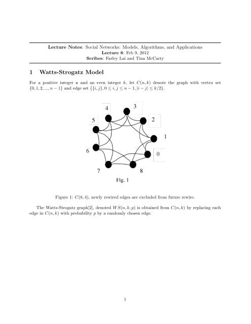
1 <strong>Watts</strong>-<strong>Strogatz</strong> <strong>Model</strong><br />
For a positive integer n and an even integer k, let C(n, k) denote the graph with vertex set<br />
{0, 1, 2, ..., n − 1} and edge set {{i, j}, 0 ≤ i, j ≤ n − 1, |i − j| ≤ k/2}.<br />
Figure 1: C(8, 4), newly rewired edges are excluded from future rewire.<br />
The <strong>Watts</strong>-<strong>Strogatz</strong> graph[2], denoted W S(n, k, p) is obtained from C(n, k) by replacing each<br />
edge in C(n, k) with probability p by a randomly chosen edge.<br />
1
Figure 2: C(P ) represents the expected clustering coefficient of W S(n, k, p). L(P ) represents the<br />
expected average path length of W S(n, k, p). It is shown that every 20 vertices receives a rewire<br />
of edges.<br />
2 Discussion<br />
Proximity. The base graph C(n, k) starts by connecting vertices that are close by. For example,<br />
Grid(n, r): vertex set {0, 1, . . . , n − 1} × {0, 1, . . . , n − 1} and edge set {(i1, j1), (i2, j2)}, where<br />
|i1 − i2| + |j1 − j2| ≤ r. An example of Grid(4, 2) is shown in Fig. 3.<br />
2
Figure 3: Grid(4, 2)<br />
It can be more abstract. Let M = (V, d) be a metric space. Consider the graph with vertex set<br />
V and edge set: {u, v : d(u, v) ≤ r}, where r is some parameter.<br />
Randomness is added in a variety of ways to achieve the same effect. Alternative Approach:<br />
start with C(n, k). To each vertex u, add an edge {u, v} with v chosen randomly.<br />
Result. This result made a lot of sense to sociologists because they believed in two types of<br />
edges:<br />
1. edges induced by homophily ⇒ base graph edges<br />
2. edges that correspond to weak ties ⇒ random edges<br />
Recall.<br />
homophily + weak ties ⇒ small world property.<br />
3
Figure 4: Alternate edges/connections may dampen the size of the set and may elongate the graph.<br />
Alternate edges/connections can also make the lengths to other edges quicker.<br />
Clustering Coefficient 1 ↑ ⇒ Average Path Length ↑<br />
Diameter. The Diameter of a Cycle Plus a Random Matching[1]. See Fig. 5. for example.<br />
1 Node based definition of clustering coefficient.<br />
4
3 Kleinberg’s Question<br />
Figure 5:<br />
<strong>Watts</strong>-<strong>Strogatz</strong> model[2] is small world. Does it also allow efficient decentralized (local) search?<br />
Example. Condider W S(n, k, p). Let s and r denote sender and receiver. The sender, knowing<br />
only r’s label, has a package that needs to be sent to r. Typical Step: node v on receiving the<br />
package, either:<br />
1. If v has a neighbor closer to r than itself, v sends the package to the neighbor closest to r.<br />
2. Otherwise, v gives up.<br />
Questions. Suppose we pick s and r randomly and perform graphic greedy routing many times:<br />
• What fraction of these experiments is successful?<br />
• What is the average path length of the successful experiments?<br />
4 Kleinberg’s <strong>Model</strong>[3]<br />
Let us use K(n, r, q, −α) to denote the graph obtained by starting with Grid(n, r) and adding<br />
random edges as follows: To each vertex u, add q random edges {u, v} with v picked out with a<br />
probability proportional to d(u, v) −α . If α = 2, then d(u, v) −α = 1/d(u, v) 2 . Fig. 6 demonstrates<br />
the model.<br />
5
Figure 6: One hop edges have higher probability to be connected than 2 or more hop edges.<br />
If α = 1, then the probability distribution is uniform such that no differentiation between near<br />
neighbors and far nodes.<br />
Results.<br />
1. For α = 0, any decentralized algorithm requires at least (n 2/3 )hops<br />
2. For α = 2, geographic greedy routing discovers paths of expected length O(log 2n)<br />
6
References<br />
Figure 7: The correlation between α and the expected path length.<br />
[1] B. Bollobs and F. R. K. Chung. The diameter of a cycle plus a random matching. SIAM J. on Discrete<br />
Mathematics, 1(3):328–333, 1998.<br />
[2] Duncan J.<strong>Watts</strong> and Steven H. <strong>Strogatz</strong>. Collective dynamics of ’small-world’ networks. Nature, 393:440–<br />
442, 1998.<br />
[3] J. Kleinberg. Navigation in a small world. Nature, 406:845, 2000.<br />
7