Prof. Dr. Wolfgang König, Prof. Dr.-Ing. Ralf ... - E-Finance Lab

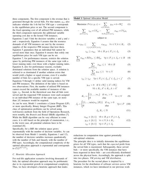
three components. The first component is the revenue that is
generated through the served bids. For that matter, yvk also
indicates whether the k-th bid for VM type v corresponds
to the equilibrium price or not. The second component is
the fixed operating cost of all utilized PM instances, while
the third component represents the additional variable
operating cost due to the hosted VM instances.
Equations 2 and 3 link the decision variables x and y and x
and z respectively. Equation 4 assures that the resource
demands of all VM instances are met by the resource
supplies of the respective PM instance that host them.
Equation 5 guarantees that an individual bid cannot be
served more than once. Equation 6 ensures that solely one
equilibrium price for each VM type can be set.
Equation 7, for performance reasons, restricts the solution
space by preferring PM instances of the same type with a
lower running index over those with a higher running index.
Equation 8, also for performance reasons, excludes
dominated solutions from the solution space. A solution is
referred to as dominated if another solution exists that
would yield a higher or equal revenue, even if a smaller
number of bids for a specific VM type is served.
Equations 9 through 11 define valid running indices for VM
and PM instances. The definition of the latter is based on
two observations: First, the number of utilized PM instances
cannot exceed the available number of instances of this
type, np. Second, in the theoretical case that all bids were
served and the requested VM instances were each assigned
to an individual PM instance of the same type, no more
than |B| instances would be required.
As can be seen, Model 1 constitutes a Linear Program (LP),
or more specifically, Binary Integer Program (BIP). This
class of optimization problems can be solved using
well-known methods from the field of Operations Research,
most notably, the Branch and Bound (B&B) algorithm [7].
While the B&B algorithm can be very efficient in some
cases, it is still based on the principle of enumeration, i. e.,
in the worst case, all potential solutions have to be
examined [8].
Specifically, for a BIP, the solution space grows
exponentially with the number of decision variables. As can
be observed from Model 1 (notably, Equations 1 and 12),
the number of decision variables increases quadratically
with the number of bids and linearly with the number of
PM types. Accordingly, the computational complexity of the
optimal allocation approach is exponential and corresponds
to O(2 |B|2 ∗|P | ).
C. Heuristic Allocation Approach
For real-life application scenarios involving thousands of
bids, the optimal allocation approach may be problematic
due to its exponential growth in computational complexity.
Thus, we have developed a heuristic approach that trades
Model 1 Optimal Allocation Model
Maximize P r(x, y, z) = �
− �
p∈P,j∈Jp
k ∗ yvk ≤
zpj ∗ CFpj −
�
1≤i≤k,p∈P,j∈Jp
v∈V,k∈Kv
�
b∈B,p∈P,j∈Jp
subject to
yvk ∗ k ∗ W v k
xbpj ∗ CVpTb
(1)
xB v i pj ∀v ∈ V, k ∈ Kv (2)
zpj ≥ xbpj ∀b ∈ B, p ∈ P, j ∈ Jp (3)
�
xbpj ∗ RDTbr ≤ RSpr ∀p ∈ P, j ∈ Jp, r ∈ R (4)
b∈B
Jp =
�
p∈P,j∈Jp
�
k∈Kv
xbpj ≤ 1 ∀b ∈ B (5)
yvk ≤ 1 ∀v ∈ V (6)
zpj ≥ zpj ′ ∀p ∈ P, j ∈ Jp, j ′ ∈ Jp, j < j ′
yvk = 0 if k ∗ W v k ≤ k ′ ∗ W v k ′
∀k ∈ Kv, k ′ ∈ Kv, k > k ′
Kv =
�
�
{1, ..., mv}
∅
if mv > 0
else
{1, ..., min(np, |B|)} if np > 0
∅ else
(7)
(8)
∀v ∈ V (9)
∀p ∈ P (10)
Jp, Kv ⊂ N (11)
xbpj ∈ {0, 1} ∀b ∈ B, p ∈ P, j ∈ Jp
yvk ∈ {0, 1} ∀v ∈ V, k ∈ Kv (12)
zpj ∈ {0, 1} ∀p ∈ P, j ∈ Jp
reductions in computation time against potentially
sub-optimal solutions.
The principle idea is to initially determine the equilibrium
prices for all VM types, such that the expected profit from
the served bids is maximized. Subsequently, these served
bids – or more specifically, the VM instances that have
been requested in these bids – are cost-efficiently distributed
across the physical hosts. Accordingly, the approach is split
into two phases, VM pricing and VM distribution.
The procedure for the second phase is inspired by a
heuristic for the distribution of software services across VM
instances, which we have introduced in our previous work