Chondrostoma nasus - Biology Centre of the Academy of Sciences of

More documents

Recommendations

Info

Water temperature (ºC) in Fischa river and Danuba river Water level Fischa river (cm) 18 16 14 12 10 8 6 4 2 0 700 600 500 400 300 200 100 Spawning area Danube 1 : 1 0 2 4 6 8 10 12 14 16 18 Water temperature (°C) in the confluence Fischa - Danube Spawning area Transition area 1 : 1 0 0 100 200 300 400 500 600 700 Water level Danube river (cm) Fig. 3. Relationship between the water temperature in the Danube River and water temperature at the spawning area in the Fischa River during spawning season (a). Relationship between the water level in the Danube River and water level at the spawning area and at the transition area in the Fischa River during spawning season (b). Pooled data of two spawning seasons. Table 1. Average water level (cm) at three sites, as well as range and variation in 2004 and 2005. 2004 2005 Spawning area (cm) Transition area (cm) Danube River (cm) Spawning area (cm) Transition area (cm) reflected peak floods during that year. The main flood peak led to a steep increase in turbidity (to approximately 10 times the average value) (Fig. 2d). (a) (b) Danube River (cm) Mean 35.9 64.0 230.7 35.9 100.6 255.0 SD 3.7 18.3 30.5 19.6 53.8 110.4 Median 35.0 55.0 228.0 31.0 80.0 274.0 Min 25.0 40.0 179.0 27.1 48.0 79.0 Max 48.0 118.0 298.0 159.4 312.0 506.0 n 70.0 70.0 70.0 65.0 65.0 65.0 mean ¼ average; SD ¼ standard deviation, Min ¼ minimum; Max ¼ maximum, n ¼ number of observations. Environmental cues in nase spawning migration In both years there was a continuous daily spawning migration in nase characterised by an oscillating pattern with several distinct peaks. In 2004, the first individuals were caught in the traps on 17 March, in 2005 recorded on 12 March. The average passage rate (±SD) between the 2 years differed significantly (Mann–Whitney U-test, P < 0.05), being 22 (±22) individualsÆday )1 in 2004 and 31 (±16) individualÆday )1 in 2005. In 2004, the highest peak of migrants was observed on 1 and 2 April (125 and 110 nase, respectively), the second highest on 13 April (56) and the third highest on 25 April (25) (Fig. 2e). The spawning migration took place to a lesser extent during the remaining sampling period. In 2005, we also observed three main migration peaks. The first immigration peak was on 16 March (48 nase), the second on 26 March (60) and the third on 7 April (81) (Fig. 2f). Highly significant correlations between daily upstream passage rate and environmental parameters like water temperature, water level and turbidity were detected (Fig. 4). In the Fischa spawning area, low water temperature (r =)0.266, P < 0.05), but especially increasing water temperature after 5 days (r = +0.430, P < 0.01), correlated significantly with the number of migrants (Fig. 4a). In 2004, a temperature increase from 5.1 to 7.0 °C in Danube and from 7.3 to 9.8 °C in the Fischa within 5 days corresponded with the trap net catch of the first four mature nase individuals. Also in the confluence (r =)0.399, P < 0.01) and in the Danube (r =)0.395, P < 0.01) low water temperatures were most significantly correlated with the migration rate. Additionally, increasing water temperature after 1 day in the confluence (r =0.273, P < 0.05) and after 3 days in the Danube (r =0.270, P < 0.05) showed significant correlation with the number of upstream migrants at the echosounder (Fig. 4b,c). At the transition area, an increased water level (r =0.424, P < 0.01) and a decreasing water level after 6 days (r =)0.299, P < 0.05) showed the highest correlations with upstream-migrating nase (Fig. 4d). In the Danube, a significant correlation was observed between an increased water level and upstream-migrating spawners (r =0.277, P < 0.05), but decreasing water level after 6 days was even more highly correlated (r =)0.312, P < 0.05) (Fig. 4e). Decreasing turbidity in the Fischa with a time lag of )6 days (r = )0.448, P < 0.01), mainly caused by decreasing water level, showed the most significant correlation with the number of upstream migrants (Fig. 4f). The water level at the spawning place and number of migrating nase were not significantly correlated. The correlation of each variable and the highest correlation of the time lags of each variable (white 507
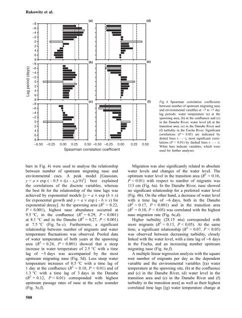
Rakowitz et al. Lag period (days) –8 –6 –4 –2 0 2 4 6 (a) (d) 8 –8 –6 –4 –2 0 2 4 6 (b) (e) 8 –8 –6 –4 –2 (c) (f) Fig. 4. Spearman correlation coefficients between number of upstream migrating nase and environmental variables at )7 to +7 day lag periods: water temperature (a) at the spawning area, (b) in the confluence and (c) 0 in the Danube River; water level (d) at the 2 transition area, (e) in the Danube River and 4 (f) turbidity in the Fischa River. Significant 6 8 –0.50 –0.25 0.00 0.25 0.50 –0.50 –0.25 0.00 0.25 0.50 Spearman correlation coefficient correlations (P =0.05) are indicated by dotted lines (……), most significant correlations (P =0.01) by dashed lines (- - - -). White bars indicate variables, which were used for further analyses. bars in Fig. 4) were used to analyse the relationship between number of upstream migrating nase and environmental cues. A peak model [Gaussian, y = a · exp ( - 0.5 · ((x - x o) ⁄ b) 2 ] best explained the correlations of the discrete variables, whereas the best fit for the relationship of the time lags was achieved by exponential models [y = a · exp (b · x) for exponential growth and y = a · exp ( - b · x) for exponential decay]. At the spawning area (R 2 = 0.22, P < 0.001), highest nase abundance occurred at 9.5 °C, in the confluence (R 2 = 0.29, P < 0.001) at 8.1 °C and in the Danube (R 2 = 0.27, P < 0.001) at 7.5 °C (Fig. 5a–c). Furthermore, a significant relationship between number of migrants and water temperature fluctuations was observed. Pooled data of water temperature of both years at the spawning area (R 2 = 0.24, P < 0.001) showed that a steep increase in water temperature of 2.5 °C with a time lag of )5 days was accompanied by the most upstream migrating nase (Fig. 5d). Less steep water temperature increases of 0.5 °C with a time lag of 1 day at the confluence (R 2 = 0.10, P < 0.01) and of 1.3 °C with a time lag of 3 days in the Danube (R 2 = 0.12, P < 0.01) corresponded with highest upstream passage rates of nase at the echo sounder (Fig. 5e,f). 508 Migration was also significantly related to absolute water levels and changes of the water level. The optimum water level in the transition area (R 2 = 0.16, P < 0.01) with respect to number of migrants was 113 cm (Fig. 6a). In the Danube River, nase showed no significant relationship for a preferred water level (Fig. 6b). On the other hand, a decrease of water level with a time lag of )6 days, both in the Danube (R 2 = 0.17, P < 0.001) and in the transition area (R 2 = 0.10, P < 0.05) was correlated with the highest nase migration rate (Fig. 6c,d). Higher turbidity (28.15 ntu) corresponded with more migrants (R 2 = 0.13, P < 0.05). At the same time, a significant relationship (R 2 = 0.07, P < 0.05) was observed between decreasing turbidity, closely linked with the water level, with a time lag of )6 days in the Fischa, and an increasing number upstream migrating nase (Fig. 6e,f). A multiple linear regression analysis with the square root number of migrants per day as the dependent variable and the environmental variables [(a) water temperature at the spawning site, (b) at the confluence and (c) in the Danube River, (d) water level in the transition area and (e) in the Danube River and (f) turbidity in the transition area] as well as their highest correlated time lags [(g) water temperature change at
Page 1 and 2: Ecology of Freshwater Fish 2008: 17
Page 3 and 4: Rakowitz et al. Materials and metho
Page 5: Rakowitz et al. all migrants in the
Page 9 and 10: Rakowitz et al. y -1 N o. of migran
Page 11 and 12: Rakowitz et al. Table 2. Summary of
Page 13: Rakowitz et al. Northcote, T.G. 198

Chondrostoma nasus - Biology Centre of the Academy of Sciences of

You also want an ePaper? Increase the reach of your titles

Delete template?

Save as template?