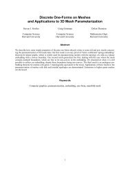
A Local/Global Approach to Mesh Parameterization

Eurographics Symposium on Geometry Processing 2008 

Pierre Alliez and Szymon Rusinkiewicz 

(Guest Editors) 

Volume 27 (2008), Number 5 

A Local/Global Approach to Mesh Parameterization 

Ligang Liu 1† Lei Zhang 1 Yin Xu 1 Craig Gotsman 2‡ Steven J. Gortler 3§ 

1 Zhejiang University, China 2 Technion, Israel 3 Harvard University, USA 

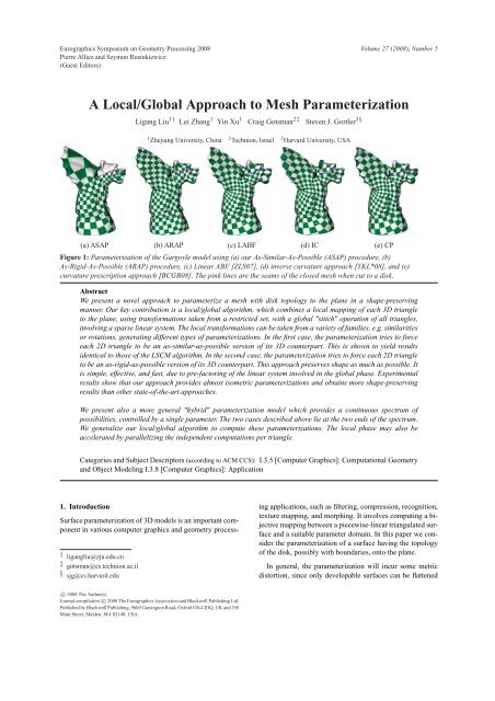
(a) ASAP (b) ARAP (c) LABF (d) IC (e) CP 

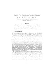
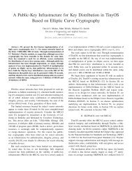
Figure 1: Parameterization of the Gargoyle model using (a) our As-Similar-As-Possible (ASAP) procedure, (b) 

As-Rigid-As-Possible (ARAP) procedure, (c) Linear ABF [ZLS07], (d) inverse curvature approach [YKL*08], and (e) 

curvature prescription approach [BCGB08]. The pink lines are the seams of the closed mesh when cut to a disk. 

Abstract 

We present a novel approach to parameterize a mesh with disk topology to the plane in a shape-preserving 

manner. Our key contribution is a local/global algorithm, which combines a local mapping of each 3D triangle 

to the plane, using transformations taken from a restricted set, with a global "stitch" operation of all triangles, 

involving a sparse linear system. The local transformations can be taken from a variety of families, e.g. similarities 

or rotations, generating different types of parameterizations. In the first case, the parameterization tries to force 

each 2D triangle to be an as-similar-as-possible version of its 3D counterpart. This is shown to yield results 

identical to those of the LSCM algorithm. In the second case, the parameterization tries to force each 2D triangle 

to be an as-rigid-as-possible version of its 3D counterpart. This approach preserves shape as much as possible. It 

is simple, effective, and fast, due to pre-factoring of the linear system involved in the global phase. Experimental 

results show that our approach provides almost isometric parameterizations and obtains more shape-preserving 

results than other state-of-the-art approaches. 

We present also a more general "hybrid" parameterization model which provides a continuous spectrum of 

possibilities, controlled by a single parameter. The two cases described above lie at the two ends of the spectrum. 

We generalize our local/global algorithm to compute these parameterizations. The local phase may also be 

accelerated by parallelizing the independent computations per triangle. 

Categories and Subject Descriptors (according to ACM CCS): I.3.5 [Computer Graphics]: Computational Geometry 

and Object Modeling I.3.8 [Computer Graphics]: Application 

1. Introduction 

Surface parameterization of 3D models is an important component 

in various computer graphics and geometry process- 

† ligangliu@zju.edu.cn 

‡ gotsman@cs.technion.ac.il 

§ sjg@cs.harvard.edu 

c○ 2008 The Author(s) 

Journal compilation c○ 2008 The Eurographics Association and Blackwell Publishing Ltd. 

Published by Blackwell Publishing, 9600 Garsington Road, Oxford OX4 2DQ, UK and 350 

Main Street, Malden, MA 02148, USA. 

ing applications, such as filtering, compression, recognition, 

texture mapping, and morphing. It involves computing a bijective 

mapping between a piecewise-linear triangulated surface 

and a suitable parameter domain. In this paper we consider 

the parameterization of a surface having the topology 

of the disk, possibly with boundaries, onto the plane. 

In general, the parameterization will incur some metric 

distortion, since only developable surfaces can be flattened

onto the plane without any distortion. Hence, the goal of parameterization 

is to find a bijective mapping which preserves 

some geometric properties of the original as much as possible, 

e.g., authalic (area-preserving) mapping, conformal 

(angle-preserving) mapping, isometric (length-preserving) 

or some combination of these. Each individual triangle may 

be easily parameterized without distortion, but then they will 

no longer fit together properly in the plane. 

Inspired by recent work on mesh deformation and modeling 

[IMH05, SA07], we formulate the parameterization 

problem as an optimization problem having both local and 

global elements. In essence, we seek for local transformations 

which minimize the distortion of each mesh triangle, 

yet require that they all fit together to a coherent 2D 

triangulation. We follow closely the method for "as-rigidas-possible" 

deformation of triangle meshes described by 

Sorkine and Alexa [SA07] for mesh editing purposes, and, 

essentially, apply the same methodology to the problem of 

mesh parameterization. 

2. Previous Work 

In the past decade, methods for triangular mesh parameterization 

have been studied extensively. We refer the interested 

reader to [FH05] and [SPR06] for a survey of the state-ofthe-art 

in parameterization research. 

The linear setting for parameterization offers the advantage 

of simplicity and validity of parameterization results. 

Based on Tutte’s barycentric mapping theorem [Tut63], Eck 

et al. [EDD ∗ 95] and Floater [Flo97] described a simple 

approach to parameterization by representing each interior 

vertex as some convex combination of its neighboring vertices. 

Depending on the precise weights used, it is possible 

to achieve a variety of effects, minimizing various distortion 

measures. The most celebrated weight recipes are 

the so-called cotangent weights [PP93], and the so-called 

mean-value weights [Flo03], which are both related to harmonic 

mappings. Unfortunately, the method of barycentric 

coordinates requires the boundary of the mesh to be fixed 

to a convex polygon in the plane, which is somewhat arbitrary, 

typically resulting in significant distortion. Lee et 

al. [LKL02] alleviated this somewhat by "padding" the mesh 

with a virtual boundary, allowing the true boundary to evolve 

to a less distorted shape. Desbrun et al. [DMA02] were 

able to generalize the method of barycentric coordinates 

so that also the boundary vertices are free, subject to socalled 

"natural" boundary conditions - some additional linear 

equations. This was shown to be equivalent to the Least- 

Squares Conformal Mapping (LSCM) method of Levy et 

al. [LPRM02], which is a least-squares approximation of the 

discrete Cauchy-Riemann equations, which define continuous 

conformal mappings. These boundary equations were 

generalized by Karni et al. [KGG05] to a larger family of 

barycentric coordinates. 

The main problem with linear free-boundary methods is 

L. Liu et al. / A Local/Global Approach to Mesh Parameterization 

that the parameterization is no longer guaranteed to be bijective, 

meaning that the resulting 2D embedding may contain 

local overlaps (also known as "triangle flips"), global overlaps, 

or even wind on itself. Karni et al. [KGG05] showed 

how to solve the more frequent problem of local overlaps in 

a postprocessing step. 

Some parameterization work focuses on directly optimizing 

the distortion metrics of length, angle or area. These 

approaches require extensive computation, since the distortion 

measures are usually highly non-linear. Hormann et 

al. [HG99] define a deformation-based MIPS energy which 

requires a non-linear solver. The compute-intensive ABF 

method of Sheffer et al. [SdS00] computes the parameterization 

in angle space, with a result minimizing angular 

distortion. The more efficient ABF++ [SLMB05] and Lin- 

ABF [ZLS07] have accelerated this method considerably. 

Other metrics are also used to guide the optimization process 

for parameterization, such as stretch. These are based 

on the singular values of the Jacobian matrix of the parameterization 

mapping [SSGH01], on the Green-Lagrange 

tensor [MYV93, ZMT05] or the synthesized distortion metric 

[YYS06]. 

Other improvements on the method of barycentric coordinates 

were proposed by Zayer et al. [ZRS05a, ZRS05b] 

and Yoshizawa et al. [YBS04], who showed how to dynamically 

adjust the barycentric weights such that the system converges 

to a parameterization minimizing stretch. 

Another approach to parameterization is inspired by recent 

advances in dimension reduction and manifold learning 

[LYD ∗ 05, ZKK02]. The basic principle is to preserve 

some geometric property like geodesic distance of a higher 

dimensional data set while embedding it in a lower dimensional 

space. For example, Chen et al. [CLZW07] introduce 

a new parameterization technique based on local tangent 

space alignment (LTSA), which tries to embed each onering 

of the mesh in some optimal manner in the plane, and 

then solves a global linear system to "stitch" the one-rings 

together to one coherent triangle mesh. In this sense, it is the 

closest to the approach we describe in this paper. 

A series of very recent works on conformal parameterizations 

by Yang et al. [YKL ∗ 08], Ben-Chen et al. [BCGB08] 

and Springborn et al. [SSP08] manipulate the curvature distribution 

on a 3D mesh, flattening it by migrating the total 

curvature so that it is distributed on only a small number of 

so-called "cone singularities". The other mesh vertices retain 

no curvature. For the case of a mesh having disk topology 

with a given boundary, this means concentrating the curvature 

on the boundary alone. In practice it amounts to computing 

new lengths for the mesh edges, so that they can be embedded 

in the plane. Once the 2D edge lengths are computed, 

the final 2D embedding is computed either by an incremental 

layout process, or by solving a simple sparse linear system 

(which happens to be identical to the LSCM process 

mentioned later in this paper, since that process reproduces 


Journal compilation c○ 2008 The Eurographics Association and Blackwell Publishing Ltd.

a planar embedding). The difference between the three methods 

is the precise algorithm used to manipulate the curvature 

distribution. These methods, although designed to minimize 

only conformal (i.e. angular) distortion, in practice produce 

parameterizations with not too much stretch. They are also 

relatively easy to compute, thus are strong contenders for use 

in conformal parameterization scenarios. 

3. Contribution 

We apply the methodology of Sorkine and Alexa [SA07] for 

mesh editing (which has its origins in a series of papers starting 

with Sorkine et al. [SCOL ∗ 04]) to the problem of mesh 

parameterization. This poses the problem as that of finding 

optimal local transformations for each individual mesh element 

from an appropriate family and then "stitching" the 

transformed triangles together to a 2D mesh. As opposed 

to [SA07], where the local transformations are applied to 

one-rings of a vertex and its neighbors, we apply the local 

transformations to individual triangles. This then becomes a 

proper finite-element discretization of an associated continuous 

problem. In this context, our contributions are: 

• For the case of local similarity transformations, our 

method is shown to be equivalent to the well known 

Least-Squares Conformal Mapping (LSCM) method 

[LPRM02]. 

• For the case of local rotational transformations, we provide 

an efficient and simple iterative "local/global" algorithm 

to solve the problem. This leads to a parameterization 

which is close to isometric and shown to be superior 

to competing algorithms. Additionally, the algorithm 

minimizes an "intrinsic" deformation energy function that 

may be expressed in terms of the singular values of the 

Jacobian of the parameterization, as is the case for many 

other distortion measures. The algorithm is shown to be 

very fast, due to pre-factoring of the linear system involved 

in the global step, and optional parallel processing 

in the local phase. 

• We propose a more general "hybrid" parameterization 

model which provides a continuous spectrum of possibilities, 

controlled by a single parameter. The two cases 

described above (similarities and rotations) lie at the two 

ends of the spectrum. The hybrid parameterization may 

also be computed using a similar local/global algorithm. 

4. The General Local/Global Approach 

If each triangle of the 3D triangle mesh were required to be 

flattened to the plane independently of the other triangles, 

this would certainly be easy. Requiring that all the flattened 

triangles fit together into one mesh with the correct orientations 

is the main challenge (see Figure 2). Obviously some 

of the triangles are going to be deformed in the process. Assume 

we allow each triangle to be deformed by some subset 

of the 2D linear transformations, in the sense that this transformation 

"does not count" as a deformation. For example, 




translations of the triangles are obviously allowed. A conformal 

parameterization would also allow each triangle to undergo 

a similarity transformation (only). An isometry would 

allow only a rotation. An authalic parameterization would 

allow only transformations with unit determinant. 

Figure 2: Parameterizing a mesh by aligning locally flattened 

triangles. (Left) Original 3D mesh; (middle) flattened 

triangles; (right) 2D parameterization. 

Assume the triangles of the 3D triangle mesh are numbered 

with t = 1 to T and the area of the 3D triangles are 

At. Assume that each 3D triangle is equipped with its own 

local isometric parameterization using a triangle in the plane 

xt = {x 0 t ,x 1 t ,x 2 t }. Our goal is to find a single parameterization 

of the entire mesh, i.e., a piecewise linear mapping from the 

3D mesh to the 2D plane, described by assigning 2D coordinates 

u to each of the n vertices. For triangle t, let us denote 

these 2D coordinates as ut = {u 0 t ,u 1 t ,u 2 t }. Given this setup, 

the mapping between xt and ut has an associated 2 × 2 Jacobian 

matrix which is constant per triangle. We denote this 

matrix at triangle t as Jt(u) to express its dependence on the 

u. It represents the linear portion of the affine mapping from 

the triangle described by xt to the triangle described by ut. 

In our method, we will also assign an auxiliary linear transformation 

(2×2 matrix) Lt to each triangle taken from some 

family of allowed transformations M (in particular, we will 

consider, in turn, M to be the similarity transformations, and 

later, the rotations). 

Define the energy of the parameterization coordinates 

u and an auxiliary set of T linear transformations L = 

{L1,..,LT } to be 

T 

E(u,L) = ∑ At �Jt(u) − Lt� 

t=1 

2 

F 

where �·� F is the Frobenius norm. Following Pinkall and 

Polthier [PP93], this energy may be rewritten in terms of the 

coordinates x and u (instead of in terms of the Jacobians) in 

an explicit form (in terms of the mesh vertex coordinates): 

E(u,L) 

= 1 T 2 

2 ∑ ∑ cot(θ 

t=1i=0 

i � 

� 

t) �(u i t − u i+1 

t ) − Lt(x i t − x i+1 

� 

� 

t ) � 2 (1) 

where θ i t is the angle opposite the edge (x i t,x i+1 

t ) in the triangle 

whose vertices are xt and superscripts are all modulo

2. Note that some of the u i t are identical, as they are shared 

by more than one triangle in the mesh. 

We would like to solve the following optimization problem: 


(u,L) = argmin (u,L) E(u,L) s.t. Lt ∈ M (2) 

Namely, find a set of n 2D coordinates u for the mesh vertices 

and T matrices L1 ,.., LT in M such that the Jacobians 

of the transformation from the given x to the u are closest to 

the Lt. 

Although we solve for both u and L, in the end we are 

interested only in u while L plays an auxiliary role only. As 

we shall see below, in many cases, the optimal u may be 

defined as that minimizing an energy function formulated in 

terms of the singular values of the Jacobians Jt(u). In the 

next sections, we will examine a number of interesting cases 

for M and relate our energy functions to those. 

4.1. Best fitting L matrix 

Suppose we are asked to approximate one 2 × 2 matrix J as 

best we can by another 2×2 matrix L, where L is taken from 

a restricted set of transformations M (we will consider in turn 

similarities and rotations) and where distance is measured 

using the Frobenius matrix norm. In other words: 

d(J,L) = �J − L� 2 

� 

F = tr (J − L) T � 

(J − L) 

This problem can be solved using Procrustes analysis 

[GD04], and its solution in general is computed using 

the Singular Value Decomposition (SVD) of J. 

In particular, using SVD, J may be written as 

J = UΣV T 

where U and V are orthonormal, and Σ is a diagonal matrix: 

� 

σ1 

Σ = 

0 

0 

σ2 

� 

We use here a "signed version" of the SVD, where the determinant 

of UV T is constrained to be positive, σ1 is positive 

and σ2 may be positive or negative. We refer to these 

σ as signed singular values. This signed version is needed 

to constrain our Procrustes solutions to exclude orientation 

reversing transformations. 

Given this decomposition, it is easy to show that the optimal 

rotation minimizing the distance d(J,L) is obtained by 

setting both singular values to 1, i.e. L = UV T . Similarly, 

the optimal similarity transform is obtained by setting both 

singular values to (σ1 + σ2)/2. See Figure 3 for examples. 

4.2. As-similar-as-possible (ASAP) mappings 

Conformal mappings are those which preserve angles, which 

are invariant under similarity transformations. Thus, in order 

to produce a conformal-type parameterization, the family 

Figure 3: Optimal Procrustes transformations: Left: source 

triangle; Right: target triangle in black, optimal similarity 

of source in red, optimal rotated version of source in green. 

M of allowed transformations should be similarities, which 

may be parameterized as all matrices of the form: 

�� 

a b 

M = 

: a,b ∈ R 

(3) 

−b a 

Thus we may represent the allowed Lt in the energy function 

(2) with the variables a = (a1,..,aT ), b = (b1,..,bT ). 

Since the x i t and θ i t are fixed, the energy function is quadratic 

in the variables a,b,u and thus may be minimized by solving 

a large sparse linear system with these variables. 

Since we try to stay close to the family of similarity 

transformations, we call this parameterization "as-similaras-possible" 

(ASAP). Appendix A proves that solving (2) 

with this M is equivalent to finding the u that minimizes 

Lévy’s conformal energy: 

T 

∑ At(σ1,t − σ2,t) 

t=1 

2 

where σ1,t and σ2,t are the signed singular values of Jt 

– the Jacobian of the t-th triangle’s transformation. Since 

the Least-Square Conformal mapping (LSCM) technique 

[LPRM02] also minimizes precisely this energy, the two 

techniques are equivalent. 

As with LSCM, for non-developable meshes, the (trivial) 

solution that collapses all of the vertices to a single point 

in the plane achieves a global minimum – zero energy. This 

can be avoided by constraining two vertices to two different 

locations in the plane. In practice, we pin down the two 

vertices most distant from each other (the diameter) in the 

mesh. 

4.3. As-rigid-as-possible (ARAP) mappings 

While conformal mappings have many nice mathematical 

properties, they are not always exactly what the application 

needs. The fact that arbitrary scaling factors may creep 

into the parameterization makes it unsuitable for applications 

which try to minimize "stretch" and preserve the proportions 

of the triangles. 

To obtain an "as-rigid-as-possible" mapping we limit the 



family of allowed local transformations to be just rotations: 

�� 

M = 

cosθ 

−sinθ 

sinθ 

cosθ 

� 

� 

: θ ∈ [0,2π) 

Or, in other words, the same as (3), only with the extra requirement 

that a 2 + b 2 = 1. 

Appendix A proves that solving (2) with this M is equivalent 

to finding the u which minimizes 

T � 

∑ At (σ1,t − 1) 

t=1 

2 + (σ2,t − 1) 2� 

This energy is similar to the Green-Lagrange energy 

� [MYV93, ZMT05], which uses terms of the form 

(σ 2 1,t − 1)2 + (σ 2 2,t − 1)2� and also produces parameterizations 

which are close to isometric. 

Alas, the extra condition on Lt in (1) means that the energy 

function may no longer be minimized by solving a linear 

system. 

4.4. Local/Global Algorithm 

To solve the minimization problem (2) for an ARAP mapping, 

we adapt the local/global algorithm of [SA07]. This 

iterates between two phases. In the first local phase, the optimal 

rotation Lt is computed per triangle, assuming the u 

are fixed. Then, in the second global phase, the Lt are assumed 

fixed, and the optimal u are solved for as a sparse 

linear system. (Recall that xt are fixed throughout the algorithm.) 

Since each step is guaranteed to reduce the energy, 

this energy will eventually converge. Additionally, since the 

matrix of the global phase is unchanged from iteration to iteration, 

it only has to be factored once and reused at each 

iteration. 

4.4.1. Local Phase 

The local phase can be solved using the SVD factorization of 

J as described in Section 4.1. Equivalently, and analogously 

to [SA07], for ARAP one can also perform the SVD factorization 

directly on the following "cross-covariance" matrix 

in place of Jt(u) 

2 

St(u) = ∑ cot(θ 

i=0 

i t)(u i t − u i+1 

t )(x i t − x i+1 

t ) T 

4.4.2. Global Phase 

For fixed Lt, the energy E(u,L) is quadratic in u. The minimum 

u can be found by setting the gradients of (1) to zero 

and solving the associated linear system. To calculate this, 

overloading the notation slightly, we rewrite the energy function 

in terms of the mesh half-edges: 




E(u,L) 

= 1 T 2 

2 ∑ ∑ cot(θ 

t=1i=0 

i � 

� 

t) �(u i t − u i+1 

t ) − Lt(x i t − x i+1 

� 

� 

t ) � 2 

= 1 � 

� 

� 

� 

2 ∑ cot(θi j) �(ui − u j) − Lt(i, j)(xi − x j) � 

(i, j)∈he 

2 

where he is the set of half-edges in the mesh, ui and xi are 

coordinates of vertices i, t(i, j) is the triangle containing the 

half-edge (i, j), and θi j is the angle opposite (i, j) in t(i, j). 

Setting the gradient to zero, we obtain the following set of 

linear equations for u. 

� 

∑ cot(θi j) + cot(θ ji) 

j∈N(i) 

� (ui − u j) 

= ∑ 

j∈N(i) 

� 

� 

cot(θi j)Lt(i, j) + cot(θ ji)Lt( j,i) (xi − x j), 

∀ i = 1,..,n. 

The entries of the associated matrix depend only on the 

geometry of the input 3D mesh. Thus this sparse matrix is 

fixed throughout the algorithm, allowing us to pre-factor it 

(e.g. with Cholesky decomposition) [GvL05, In0] and reuse 

the factorization many times throughout the algorithm in order 

to accelerate the process. This has a significant impact 

on algorithm efficiency. 

Unfortunately, stitching the triangles using a global Poisson 

equation may result in some triangles "flipping" their 

orientation especially for a highly curved surface with compact 

boundary. We solve this with a final post-processing 

phase, e.g., the "convex virtual boundary" algorithm of Karni 

et al. [KGG05]. Since in most cases, there are only a few 

flips, sprinkled throughout the parameterization, the postprocessing 

solves the flips without changing much else. 

4.5. The initial parameterization 

Our local/global algorithm requires an initial parameterization 

M to start it off. The basic requirement from the initial 

parameterization is that it be a valid embedding (contain 

no flips) reasonably close to a parameterization with not 

too much distortion, and be fast to generate. Candidates are 

the shape-preserving method [Flo97] and LSCM [LPRM02] 

as they can be computed quickly. We found the shapepreserving 

parameterization more suitable for meshes with 

one boundary, and LSCM [LPRM02] for meshes with multiple 

boundaries. The experimental results shown in Section 

6 are obtained using these initial parameterizations. 

We tested the sensitivity of our algorithm to different 

types of M’s, as mentioned above. We found that the algorithm 

is not sensitive to M at all. Figure 4 shows the progress 

of the iterative algorithm when initialized with the shapepreserving 

parameterization and LSCM. Both converge fast 

and stably. 

(4)


Initial guess 1 Iteration 3 Iterations Final result 

Figure 4: Successive iterations of the local/global ARAP algorithm. (Top) Initialized using Floater’s shape-preserving parameterization 

[Flo97]. (Bottom) Lower row: Initialized using LSCM parameterization [LPRM02]. 

5. The Hybrid Model 

Our ASAP parameterization belongs to the family of (approximately) 

conformal maps and may be computed easily 

by solving a simple linear system. However, it is not 

the most area-preserving among the conformal parameterizations, 

and, in fact, the non-linear ABF++ method preserves 

area much better, while still being approximately conformal. 

On the other hand, our ARAP parameterization preserves areas 

much better, but since it it strives to be isometric, it might 

damage the conformality in this effort. We now present an 

energy function which is a generalization of (1), which provides 

a means to generate a parameterization anywhere between 

ASAP and ARAP. The two latter are endpoints of 

the spectrum, and the result is controlled by a parameter 

λ ∈ [0,∞). 

The hybrid energy function is 

E(u,a,b) 

� 

= 

T 2 

1 

2 ∑ ∑ cot(θ 

t=1 i=0 

i � 

� 

t) �∇e i � 

� 

t� 

2 

+ λ(a 2 t + b 2 t − 1) 2 

� 

, 

where 

∇e i t = (u i t − u i+1 

� 

at bt 

t ) − 

−bt at 

� 

(x i t − x i+1 

t ). 

Setting λ=0 will be equivalent to ASAP while a very large 

value of λ will be equivalent to ARAP. Any value inbetween 

will yield an intermediate parameterization, so the 

user may control the tradeoff between conformality and 

area-preservation. 

(5) 

Solving for the parameterization coordinates u which 

minimize E(u,a,b) involves solving also for the auxiliary 

vectors of unknowns of the similarity transformations a and 

b. The value of λ indicates how much we want to force the 

similarity to be a rotation. A local/global algorithm similar to 

that we use for solving for the ARAP parameterization may 

be used here as well, i.e. iterate while alternating between 

two phases: one local and one global. Recall that x is fixed 

(derived directly from the input 3D mesh). The local phase 

keeps the parameterization coordinates u fixed and solves for 

the optimal at and bt per triangle t. Examination of (5) reveals 

that this involves solving two cubic equations in at and 

bt. Furthermore, this reduces to a single cubic equation in at, 

(Equation (B3) in Appendix B), which may be solved analytically. 

The global phase keeps both vectors a and b fixed 

and solves a global sparse linear system (similar to (4)) for 

u. Since the matrix of the linear system is fixed throughout 

all iterations, it may be pre-factored at the beginning, and 

reused in all iterations thereafter. Thus the runtime of the 

procedure is dominated by the first iteration. This makes for 

a simple and efficient algorithm. 

6. Experimental Results and Comparison 

We have applied our approach to parameterize a variety 

of 3D meshes and compared with other relevant methods. 

These include LSCM (equivalent to our ASAP method) 

[LPRM02], direct ABF++ (ABF++ without the hierarchical 

solver) [SLMB05], which we label dABF++, linear 

ABF [ZLS07], which we label LABF, inverse curvature 



ASAP (¡ =0) 

(2.05, 15.4) 

=0.0001 

(2.05, 5.74) 


=0.001 

(2.07, 2.88) 

=0.1 

(2.18, 2.14) 

ARAP ( =∞) 

(2.19, 2.11) 

LABF 

(2.12, 9.12) 

IC 

(3.09, 3.91) 

CP 

(2.29, 11.9) 

Figure 5: Isis model: Effect of λ in hybrid energy function (5) compared with results of other algorithms. Numbers in brackets 

denote angular distortion and area distortion. 

ASAP ( =0) (2.02, 2.42) 

=10 -4 (2.02, 2.31) 

ARAP (¡ =∞) (2.07, 2.04) LABF (2.05, 2.34) 

=10 -3 (2.03, 2.15) 

=10 -1 (2.07, 2.05) 

IC (2.06, 2.42) CP (2.36, 3.18) 

Figure 6: Balls model: Effect of λ in hybrid energy function (5) compared with results of other algorithms. Numbers in brackets 

denote angular distortion and area distortion. 

[YKL ∗ 08], which we label IC, and curvature prescription 

[BCGB08], which we label CP. We show some results in 

Fig. 1 and Figs. 5-8. In our algorithm, we used the sparse 

Cholesky linear solver [In0] for the global systems and the 

analytic solution to Equation (B3) for the local systems. The 

IC results were kindly provided by Yang and the CP results 

by Ben-Chen, the authors of those methods, who ran their 

own software. The results of LABF where obtained by running 

software kindly provided by Zayer. 

Computing the ASAP parameterization involves the solution 

of one sparse linear system, thus is very fast. Computing 

ARAP involves running the local/global algorithm. This 

converged in up to 10 iterations in all our experiments. Computing 

the hybrid also involves an iterative local/global algo- 



rithm, but with the local phase using the analytic solution to 

Equation (B3) instead of a simple 2 × 2 SVD operation. 

The figures show the parameterizations resulting from 

ASAP, ARAP and the hybrid method with some interesting 

values of λ. These are compared with the results of 

the other algorithms. The runtime of our local/global procedure 

is comparable to the state-of-the-art ABF++. Our local/global 

parameterization method may be applied also to 

meshes with multiple boundaries. Fig. 8 shows one such result. 

The LABF method is not applicable to such inputs. 

To quantify the parameterization distortion, we compute 

both the angle and area distortion metric defined using the 

signed singular values σ1,t and σ2,t of the Jacobians Jt for


ASAP ARAP 

dABF++ 

LABF 

IC 

Figure 7: Cow model: Comparison with other algorithms. The pink lines are the seams of the closed mesh when cut to a disk. 

Triangulations are the 2D parameterizations. 

dABF++ 

ARAP 

Figure 8: Beetle model with multiple boundaries: (Left) Direct 

ABF++. (Right) ARAP. 

each triangle, as defined in [HG99, DMK03]: 

D angle � 

= ∑ρt σ 

t 

1 t /σ 2 t + σ 2 t /σ 1 � 

t 

D area � 

= ∑ρt σ 

t 

1 t σ 2 t + 1/(σ 1 t σ 2 � 

t ) 

where the weight ρt is 

ρt = At/∑At t 

and At is the area of triangle t. The values of the distortion 

measures obtained by the various algorithms is summarized 

in Table 1. As is evident in the table, our ARAP parameterization 

consistently gives the best value of D area , at a very 

small, even insignificant, penalty in D angle . It is possible to 

significantly improve the value of D area relative to LSCM 

even by introducing a small value of λ. 

7. Discussion and Conclusion 

We have presented a novel approach to parameterization of 

3D mesh surfaces, by minimizing a very general energy 

function. We have also provided a simple and efficient local/global 

algorithm for computing these parameterizations. 

The local component of the algorithm tries to minimize distortion 

of the individual 2D triangles relative to the original 

3D mesh geometry, while the global component guarantees 

that the resulting 2D triangles fit together in a coherent 

manner. Both phases may be computed efficiently, the local 

one taking advantage of parallelism (possibly on the GPU), 

and the global one taking advantage of efficient sparse linear 

solvers with factorization. 

We have shown that our ASAP definition is equivalent 

to LSCM, while ARAP can yield more shape-preserving 

results compared with other contemporary methods. A hybrid 

model, coupled with a similar efficient local/global algorithm, 

allows to obtain parameterizations anywhere inbetween 

these two. While we have applied this method to 

parameterizing meshes with disk topology only, it seems it 

could be possible to use the same methodology for higher 

genus meshes, possibly through the use of one-forms. Positional 

constraints on some of the vertices in parameter space 

can also be imposed without complicating the algorithm, as 

these types of (hard or soft) constraints may be easily incorporated 

into the energy functions we optimize. 



CP


Table 1: Comparison of distortion measures of different parameterization methods. 

D angle 

D area 

Model 

LSCM dABF LABF IC CP ARAP LSCM dABF LABF IC CP ARAP 

Gargoyle 2.00 2.00 2.00 2.05 2.00 2.06 88.14 2.64 2.64 2.67 2.64 2.05 

Isis 2.05 2.08 2.12 3.09 2.29 2.19 15.36 8.37 9.12 3.91 11.94 2.11 

Balls 2.02 2.06 2.05 2.06 2.36 2.07 2.40 2.35 2.34 2.42 3.18 2.04 

Cow 2.01 2.01 2.01 2.46 2.01 2.03 30.09 2.19 2.22 2.51 2.18 2.03 

Beetle 2.00 2.00 - 2.02 2.00 2.01 2.08 2.09 - 2.14 2.10 2.01 

Our local/global algorithm embodies the motif "think 

globally, act locally", which is emerging as a powerful technique 

in geometry processing. This paper and others [DG07] 

have applied this to the problem of mesh parameterization 

and future work will address other applications where the 

technique may also be very effective. 

Acknowledgements 

Thanks to Yongliang Yang and Miri Ben-Chen for providing results 

of the algorithms of [YKL ∗ 08] and [BCGB08]. Thanks also 

to Hugues Hoppe for his many helpful insights on this topic. This 

work is supported by National Natural Science Foundation of China 

(grants # 60776799, 60503067). Craig Gotsman and Steven Gortler 

were partially supported by United States - Israel Binational Science 

Foundation grant # 2006089. 

References 

[BCGB08] BEN-CHEN M., GOTSMAN C., BUNIN G.: Conformal 

flattening by curvature prescription and metric scaling. Computer 

Graphics Forum 27, 2 (2008), 449–458. (Proc. Eurographics 

2008). 2, 7, 9 

[CLZW07] CHEN Z. G., LIU L. G., ZHANG Z. Y., WANG G. J.: 

Surface parameterization via aligning optimal local flattening. 

In Proc. Symposium on Solid and Physical Modeling (2007), 

pp. 291–296. 2 

[DG07] DONG S., GARLAND M.: Iterative methods for improving 

mesh parameterizations. In Proc. IEEE Shape Modeling International 

(2007), pp. 119–210. 9 

[DMA02] DESBRUN M., MEYER M., ALLIEZ P.: Intrinsic parameterization 

of surface meshes. Computer Graphics Forum 21, 

3 (2002), C209–C218. (Proc. Eurographics’02). 2 

[DMK03] DEGENER P., MESETH J., KLEIN R.: An adaptable 

surface parameterization method. In Proc. of 12th International 

Meshing Roundtable (2003), pp. 227–237. 8 

[EDD ∗ 95] ECK M., DEROSE T., DUCHAMP T., HOPPE H., 

LOUNSBERY M., STUETZLE W.: Multiresolution analysis of 

arbitrary meshes. In Proc. Siggraph’95 (1995), pp. 173–182. 2 

[FH05] FLOATER M. S., HORMANN K.: Surface parameterization: 

a tutorial and survey. In Advances in Multiresolution for 

Geometric Modeling (2005), pp. 157–186. 2 

[Flo97] FLOATER M. S.: Parameterization and smooth approximation 

of surface triangulations. Computer Aided Geometry Design 

14 (1997), 231–250. 2, 5 



[Flo03] FLOATER M.: Mean value coordinates. Computer Aided 

Geometric Design 20, 1 (2003), 19–27. 2 

[GD04] GOWER J. C., DIJKSTERHUIS G. B.: Procrustes Problems. 

Oxford University Press, 2004. 4 

[GvL05] GOLUB G. H., VAN LOAN C. F.: Matrix Computation. 

Johns Hopkins Studies in Mathematical Sciences, 2005. 5 

[HG99] HORMANN K., GREINER G.: MIPS: an efficient global 

parameterization method. In Proc. Curves and Surfaces (1999), 

pp. 153–162. 2, 8 

[IMH05] IGARASHI T., MOSCOVICH T., HUGHES J. F.: Asrigid-as-possible 

shape manipulation. ACM TOG 24, 3 (2005), 

C1134–C1141. (Proc. Siggraph’05). 2 

[In0] Intel math kernel library. http://developer.intel.com. 

5, 7 

[KGG05] KARNI Z., GOTSMAN C., GORTLER S. J.: Freeboundary 

linear parameterization of 3D meshes in the presence 

of constraints. In Proc. IEEE Shape Modeling and Applications 

(2005), pp. 268–277. 2, 5 

[LKL02] LEE Y., KIM H. S., LEE S.: Mesh parameterization 

with a virtual boundary. Computer and Graphics 26, 5 (2002), 

677–686. 2 

[LPRM02] LÉVY B., PETITJEAN S., RAY N., MAILLOT J.: 

Least squares conformal maps for automatic texture atlas generation. 

ACM TOG 21, 3 (2002), C362–C371. (Proc. Siggraph’02). 

2, 3, 4, 5, 6, 10 

[LYD ∗ 05] LIU Y. S., YU P. Q., DU M. C., YONG J. H., ZHANG 

H., PAUL J. C.: Mesh parameterization for an open connected 

surface without partition. In Proc. of Computer Aided Design 

and Computer Graphics (2005), pp. 306–312. 2 

[MYV93] MAILLOT J., YAHIA H., VERROUST A.: Interactive 

texture mapping. In Proc. Siggraph’93 (1993), pp. 27–34. 2, 5 

[PP93] PINKALL U., POLTHIER K.: Computing discrete minimal 

surface and their conjugates. Experimental Mathematics 2, 

1 (1993), 15–36. 2, 3 

[SA07] SORKINE O., ALEXA M.: As-rigid-as-possible surface 

modeling. In Proc. Eurographics Symposium on Geometry Processing 

(2007), pp. 109–116. 2, 3, 5 

[SCOL ∗ 04] SORKINE O., COHEN-OR D., LIPMAN Y., ALEXA 

M., ROESSL C., SEIDEL H.-P.: Laplacian surface editing. In 

Proc. Eurographics Symposium on Geometry Processing (2004), 

pp. 175–184. 3 

[SdS00] SHEFFER A., DE STURLER E.: Parameterization of 

faceted surfaces for meshing using angle-based flattening. Engineering 

with Computer 17, 3 (2000), 326–337. 2

[SLMB05] SHEFFER A., LÉVY B., MOGILNITSKY M., BO- 

GOMYAKOV A.: ABF++: Fast and robust angle-based flattening. 

ACM TOG 24, 2 (2005), 311–330. 2, 6 

[SPR06] SHEFFER A., PRAUN E., ROSE K.: Mesh parameterization 

methods and their applications. Foundation and Trends in 

Computer Graphics and Vision 2, 2 (2006), 105–171. 2 

[SSGH01] SANDER P. V., SNYDER J., GORTER S. J., HOPPE 

H.: Texture mapping progressive meshes. In Proc. SIGGRAPH 

’01 (2001), pp. 409–416. 2 

[SSP08] SPRINGBORN B., SCHROEDER P., PINKALL U.: Conformal 

equivalence of triangle meshes. ACM Transactions on 

Graphics 27, 3 (2008). (Proc. SIGGRAPH 2008). 2 

[Tut63] TUTTE W.: How to draw a graph. In Proc. London Mathematical 

Society (1963), pp. 743–768. 2 

[YBS04] YOSHIZAWA S., BELYAEV A. G., SEIDEL H.-P.: A 

fast and simple stretch-minimizing mesh parameterization. In 

Proc. Shape Modeling International (2004), pp. 200–208. 2 

[YKL ∗ 08] YANG Y., KIM J., LUO F., HU S., GU X.: Optimal 

surface parameterization using inverse curvature map. IEEE 

TVCG (2008). To appear. 2, 7, 9 

[YYS06] YAN J. Q., YANG X., SHI P. F.: Mesh parameterization 

by minimizing the synthesized distortion metric with the coefficient 

optimizing algorithm. IEEE Transactions on Visualization 

and Computer Graphics 12, 1 (2006), 83–92. 2 

[ZKK02] ZIGELMAN G., KIMMEL R., KIRYATI N.: Texture 

mapping using surface flattening via multidimensional scaling. 

IEEE Transactions on Visualization and Computer Graphics 8, 2 

(2002), 198–207. 2 

[ZLS07] ZAYER R., LÉVY B., SEIDEL H.-P.: Linear angle based 

parameterization. In Proc. Eurographics Symposium on Geometry 

Processing (2007), pp. 135–141. 2, 6 

[ZMT05] ZHANG E., MISCHAIKOW K., TURK G.: Featurebased 

surface parameterization and texture mapping. ACM TOG 

24, 1 (2005), 1–27. 2, 5 

[ZRS05a] ZAYER R., ROESSL C., SEIDEL H.-P.: Discrete tensorial 

quasi-harmonic maps. In Proc. IEEE Shape Modeling and 

Applications (2005), pp. 278–287. 2 

[ZRS05b] ZAYER R., ROESSL C., SEIDEL H.-P.: Setting the 

boundary free: A composite approach to surface parameterization. 

In Proc. Eurographics Symposium on Geometry Processing 

(2005), pp. 91–100. 2 

Appendix A: 

Consider minimizing the following energy function 

subject to Lt ∈ M. 

T 

E(u,L) = ∑At 

�Jt(u) − Lt� 

t=1 

2 

F 


T 

= ∑Attr 

t=1 

� (Jt(u) − Lt) T (Jt(u) − Lt) � 

(A1) 

If we define E(u) = minLE(u,L), then our optimization becomes 

minu E(u). To understand E(u), we use the fact that for a fixed u, 

the best Lt for each triangle can be expressed using Procrustes analysis. 

In particular, if by the signed SVD, Jt = UtΣtV T 

t , for Σt = 

� � 

σ1,t 0 

, then the optimal Lt is of the form Lt = UtKtV 

0 σ2,t 

T 

t , 

� � 

k1,t 0 

for Kt = 

where for the ARAP case, k1,t = k2,t = 1, 

0 k2,t 

and for the ASAP case, k1,t = k2,t = (σ1,t + σ2,t)/2. 

Substituting this in (A1), we get 

E(u) 

T 

= ∑Attr 

t=1 

� (UtΣtV T 

t −UtKtV T 

t ) T (UtΣtV T 

t −UtKtV T 

t ) � 

T 

= ∑Attr(VtΣ 

t=1 

2 t V T 

t − 2VtΣtKtV T 

t +VtK 2 t V T 

t ) 

T 

= ∑Attr(Σ 

t=1 

2 t − 2ΣtKt + K 2 t ) 

T � 

= ∑ At (σ1,t − k1,t) 

t=1 

2 + (σ2,t − k2,t) 2� 

In particular, for the ARAP case, k1,t = k2,t = 1, so 

T � 

E(u) = ∑At 

(σ1,t − 1) 

t=1 

2 + (σ2,t − 1) 2� 

. (A2) 

and for the ASAP case, k1,t = k2,t = (σ1,t + σ2,t)/2, so 

T 

E(u) = ∑At(σ1,t 

− σ2,t) 

t=1 

2 , (A3) 

which has been shown to be identical to Lévy’s conformal energy 

[LPRM02], minimized by the LSCM algorithm. 

Appendix B: 

Assume we seek a and b minimizing 

2 � 

E(a,b) = ∑wi 

�∇e 

i=0 

i�� 2 + λ(a 2 + b 2 − 1) 2 

where ∇ei = (ui − ui+1 � 

) − 

a 

−b 

b 

a 

� 

(vi − vi+1 ) and all other 

quantities are constants. 

Denote ui − ui+1 � 

∇ui x = 

∇ui y 

� 

,vi − vi+1 � 

∇vi x = 

∇vi y 

� 

. Taking 

∂E/∂a = 0 and ∂E/∂b = 0 yields: 

C1a + 2λa(a 2 + b 2 − 1) = C2 

. 

(B1) 

C1b + 2λb(a 2 + b 2 − 1) = C3 

(B2) 

where C1 = ∑ 2 i=0 wi 

� 

(∇vi x ) 2 + (∇vi y )2� , 

C2 = ∑ 2 i=0 wi 

� 

∇ui x∇vi x + ∇ui y∇vi � 

y , C3 = 

∑ 2 i=0 wi 

� 

∇ui x∇vi y − ∇ui y∇vi � 

x . 

Dividing (B1) by (B2) gives b = (C3/C2)a, and the final cubic 

equation in a: 

2λ(C2 2 +C2 3 ) 

C2 a 

2 

3 + (C1 − 2λ)a −C2 = 0 (B3) 

For the special case λ = 0 it is easy to derive the solutions 

and for the special case λ → ∞ 

a = C2 

, b = 

C1 

C3 

C1 

a = ± � 

C2 

C2 2 +C2 , b = ± � 

C3 

3 

C2 2 +C2 3

A Local/Global Approach to Mesh Parameterization

You also want an ePaper? Increase the reach of your titles

Delete template?

Save as template?