Column-Stores vs. Row-Stores - MIT Database Group

Column-Stores vs. Row-Stores: How Different Are They 

Really? 

ABSTRACT 

Daniel J. Abadi 

Yale University 

New Haven, CT, USA 

dna@cs.yale.edu 

There has been a significant amount of excitement and recent work 

on column-oriented database systems (“column-stores”). These 

database systems have been shown to perform more than an order 

of magnitude better than traditional row-oriented database systems 

(“row-stores”) on analytical workloads such as those found in 

data warehouses, decision support, and business intelligence applications. 

The elevator pitch behind this performance difference is 

straightforward: column-stores are more I/O efficient for read-only 

queries since they only have to read from disk (or from memory) 

those attributes accessed by a query. 

This simplistic view leads to the assumption that one can obtain 

the performance benefits of a column-store using a row-store: 

either by vertically partitioning the schema, or by indexing every 

column so that columns can be accessed independently. In this paper, 

we demonstrate that this assumption is false. We compare the 

performance of a commercial row-store under a variety of different 

configurations with a column-store and show that the row-store 

performance is significantly slower on a recently proposed data 

warehouse benchmark. We then analyze the performance difference 

and show that there are some important differences between 

the two systems at the query executor level (in addition to the obvious 

differences at the storage layer level). Using the column-store, 

we then tease apart these differences, demonstrating the impact on 

performance of a variety of column-oriented query execution techniques, 

including vectorized query processing, compression, and a 

new join algorithm we introduce in this paper. We conclude that 

while it is not impossible for a row-store to achieve some of the 

performance advantages of a column-store, changes must be made 

to both the storage layer and the query executor to fully obtain the 

benefits of a column-oriented approach. 

Categories and Subject Descriptors 

H.2.4 [Database Management]: Systems—Query processing, Relational 

databases 

Permission to make digital or hard copies of all or part of this work for 

personal or classroom use is granted without fee provided that copies are 

not made or distributed for profit or commercial advantage and that copies 

bear this notice and the full citation on the first page. To copy otherwise, to 

republish, to post on servers or to redistribute to lists, requires prior specific 

permission and/or a fee. 

SIGMOD’08, June 9–12, 2008, Vancouver, BC, Canada. 

Copyright 2008 ACM 978-1-60558-102-6/08/06 ...$5.00. 

Samuel R. Madden 

MIT 

Cambridge, MA, USA 

madden@csail.mit.edu 

1 

General Terms 

Nabil Hachem 

AvantGarde Consulting, LLC 

Shrewsbury, MA, USA 

nhachem@agdba.com 

Experimentation, Performance, Measurement 

Keywords 

C-Store, column-store, column-oriented DBMS, invisible join, compression, 

tuple reconstruction, tuple materialization. 

1. INTRODUCTION 

Recent years have seen the introduction of a number of columnoriented 

database systems, including MonetDB [9, 10] and C-Store [22]. 

The authors of these systems claim that their approach offers orderof-magnitude 

gains on certain workloads, particularly on read-intensive 

analytical processing workloads, such as those encountered in data 

warehouses. 

Indeed, papers describing column-oriented database systems usually 

include performance results showing such gains against traditional, 

row-oriented databases (either commercial or open source). 

These evaluations, however, typically benchmark against row-oriented 

systems that use a “conventional” physical design consisting of 

a collection of row-oriented tables with a more-or-less one-to-one 

mapping to the tables in the logical schema. Though such results 

clearly demonstrate the potential of a column-oriented approach, 

they leave open a key question: Are these performance gains due 

to something fundamental about the way column-oriented DBMSs 

are internally architected, or would such gains also be possible in 

a conventional system that used a more column-oriented physical 

design? 

Often, designers of column-based systems claim there is a fundamental 

difference between a from-scratch column-store and a rowstore 

using column-oriented physical design without actually exploring 

alternate physical designs for the row-store system. Hence, 

one goal of this paper is to answer this question in a systematic 

way. One of the authors of this paper is a professional DBA specializing 

in a popular commercial row-oriented database. He has 

carefully implemented a number of different physical database designs 

for a recently proposed data warehousing benchmark, the Star 

Schema Benchmark (SSBM) [18, 19], exploring designs that are as 

“column-oriented” as possible (in addition to more traditional designs), 

including: 

• Vertically partitioning the tables in the system into a collection 

of two-column tables consisting of (table key, attribute) 

pairs, so that only the necessary columns need to be read to 

answer a query. 

• Using index-only plans; by creating a collection of indices 

that cover all of the columns used in a query, it is possible

for the database system to answer a query without ever going 

to the underlying (row-oriented) tables. 

• Using a collection of materialized views such that there is a 

view with exactly the columns needed to answer every query 

in the benchmark. Though this approach uses a lot of space, 

it is the ‘best case’ for a row-store, and provides a useful 

point of comparison to a column-store implementation. 

We compare the performance of these various techniques to the 

baseline performance of the open-source C-Store database [22] on 

the SSBM, showing that, despite the ability of the above methods 

to emulate the physical structure of a column-store inside a rowstore, 

their query processing performance is quite poor. Hence, one 

contribution of this work is showing that there is in fact something 

fundamental about the design of column-store systems that makes 

them better suited to data-warehousing workloads. This is important 

because it puts to rest a common claim that it would be easy 

for existing row-oriented vendors to adopt a column-oriented physical 

database design. We emphasize that our goal is not to find the 

fastest performing implementation of SSBM in our row-oriented 

database, but to evaluate the performance of specific, “columnar” 

physical implementations, which leads us to a second question: 

Which of the many column-database specific optimizations proposed 

in the literature are most responsible for the significant performance 

advantage of column-stores over row-stores on warehouse 

workloads? 

Prior research has suggested that important optimizations specific 

to column-oriented DBMSs include: 

• Late materialization (when combined with the block iteration 

optimization below, this technique is also known as vectorized 

query processing [9, 25]), where columns read off disk 

are joined together into rows as late as possible in a query 

plan [5]. 

• Block iteration [25], where multiple values from a column 

are passed as a block from one operator to the next, rather 

than using Volcano-style per-tuple iterators [11]. If the values 

are fixed-width, they are iterated through as an array. 

• Column-specific compression techniques, such as run-length 

encoding, with direct operation on compressed data when using 

late-materialization plans [4]. 

• We also propose a new optimization, called invisible joins, 

which substantially improves join performance in late-materialization 

column stores, especially on the types of schemas 

found in data warehouses. 

However, because each of these techniques was described in a 

separate research paper, no work has analyzed exactly which of 

these gains are most significant. Hence, a third contribution of 

this work is to carefully measure different variants of the C-Store 

database by removing these column-specific optimizations one-byone 

(in effect, making the C-Store query executor behave more like 

a row-store), breaking down the factors responsible for its good performance. 

We find that compression can offer order-of-magnitude 

gains when it is possible, but that the benefits are less substantial in 

other cases, whereas late materialization offers about a factor of 3 

performance gain across the board. Other optimizations – including 

block iteration and our new invisible join technique, offer about 

a factor 1.5 performance gain on average. 

In summary, we make three contributions in this paper: 

2 

1. We show that trying to emulate a column-store in a row-store 

does not yield good performance results, and that a variety 

of techniques typically seen as ”good” for warehouse performance 

(index-only plans, bitmap indices, etc.) do little to 

improve the situation. 

2. We propose a new technique for improving join performance 

in column stores called invisible joins. We demonstrate experimentally 

that, in many cases, the execution of a join using 

this technique can perform as well as or better than selecting 

and extracting data from a single denormalized table 

where the join has already been materialized. We thus 

conclude that denormalization, an important but expensive 

(in space requirements) and complicated (in deciding in advance 

what tables to denormalize) performance enhancing 

technique used in row-stores (especially data warehouses) is 

not necessary in column-stores (or can be used with greatly 

reduced cost and complexity). 

3. We break-down the sources of column-database performance 

on warehouse workloads, exploring the contribution of latematerialization, 

compression, block iteration, and invisible 

joins on overall system performance. Our results validate 

previous claims of column-store performance on a new data 

warehousing benchmark (the SSBM), and demonstrate that 

simple column-oriented operation – without compression and 

late materialization – does not dramatically outperform welloptimized 

row-store designs. 

The rest of this paper is organized as follows: we begin by describing 

prior work on column-oriented databases, including surveying 

past performance comparisons and describing some of the 

architectural innovations that have been proposed for column-oriented 

DBMSs (Section 2); then, we review the SSBM (Section 3). We 

then describe the physical database design techniques used in our 

row-oriented system (Section 4), and the physical layout and query 

execution techniques used by the C-Store system (Section 5). We 

then present performance comparisons between the two systems, 

first contrasting our row-oriented designs to the baseline C-Store 

performance and then decomposing the performance of C-Store to 

measure which of the techniques it employs for efficient query execution 

are most effective on the SSBM (Section 6). 

2. BACKGROUND AND PRIOR WORK 

In this section, we briefly present related efforts to characterize 

column-store performance relative to traditional row-stores. 

Although the idea of vertically partitioning database tables to 

improve performance has been around a long time [1, 7, 16], the 

MonetDB [10] and the MonetDB/X100 [9] systems pioneered the 

design of modern column-oriented database systems and vectorized 

query execution. They show that column-oriented designs – 

due to superior CPU and cache performance (in addition to reduced 

I/O) – can dramatically outperform commercial and open 

source databases on benchmarks like TPC-H. The MonetDB work 

does not, however, attempt to evaluate what kind of performance 

is possible from row-stores using column-oriented techniques, and 

to the best of our knowledge, their optimizations have never been 

evaluated in the same context as the C-Store optimization of direct 

operation on compressed data. 

The fractured mirrors approach [21] is another recent columnstore 

system, in which a hybrid row/column approach is proposed. 

Here, the row-store primarily processes updates and the columnstore 

primarily processes reads, with a background process migrating 

data from the row-store to the column-store. This work

also explores several different representations for a fully vertically 

partitioned strategy in a row-store (Shore), concluding that tuple 

overheads in a naive scheme are a significant problem, and that 

prefetching of large blocks of tuples from disk is essential to improve 

tuple reconstruction times. 

C-Store [22] is a more recent column-oriented DBMS. It includes 

many of the same features as MonetDB/X100, as well as 

optimizations for direct operation on compressed data [4]. Like 

the other two systems, it shows that a column-store can dramatically 

outperform a row-store on warehouse workloads, but doesn’t 

carefully explore the design space of feasible row-store physical 

designs. In this paper, we dissect the performance of C-Store, noting 

how the various optimizations proposed in the literature (e.g., 

[4, 5]) contribute to its overall performance relative to a row-store 

on a complete data warehousing benchmark, something that prior 

work from the C-Store group has not done. 

Harizopoulos et al. [14] compare the performance of a row and 

column store built from scratch, studying simple plans that scan 

data from disk only and immediately construct tuples (“early materialization”). 

This work demonstrates that in a carefully controlled 

environment with simple plans, column stores outperform 

row stores in proportion to the fraction of columns they read from 

disk, but doesn’t look specifically at optimizations for improving 

row-store performance, nor at some of the advanced techniques for 

improving column-store performance. 

Halverson et al. [13] built a column-store implementation in Shore 

and compared an unmodified (row-based) version of Shore to a vertically 

partitioned variant of Shore. Their work proposes an optimization, 

called “super tuples”, that avoids duplicating header information 

and batches many tuples together in a block, which can 

reduce the overheads of the fully vertically partitioned scheme and 

which, for the benchmarks included in the paper, make a vertically 

partitioned database competitive with a column-store. The paper 

does not, however, explore the performance benefits of many recent 

column-oriented optimizations, including a variety of different 

compression methods or late-materialization. Nonetheless, the 

“super tuple” is the type of higher-level optimization that this paper 

concludes will be needed to be added to row-stores in order to 

simulate column-store performance. 

3. STAR SCHEMA BENCHMARK 

In this paper, we use the Star Schema Benchmark (SSBM) [18, 

19] to compare the performance of C-Store and the commercial 

row-store. 

The SSBM is a data warehousing benchmark derived from TPC- 

H 1 . Unlike TPC-H, it uses a pure textbook star-schema (the “best 

practices” data organization for data warehouses). It also consists 

of fewer queries than TPC-H and has less stringent requirements on 

what forms of tuning are and are not allowed. We chose it because 

it is easier to implement than TPC-H and we did not have to modify 

C-Store to get it to run (which we would have had to do to get the 

entire TPC-H benchmark running). 

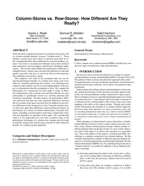
Schema: The benchmark consists of a single fact table, the LINE- 

ORDER table, that combines the LINEITEM and ORDERS table of 

TPC-H. This is a 17 column table with information about individual 

orders, with a composite primary key consisting of the ORDERKEY 

and LINENUMBER attributes. Other attributes in the LINEORDER 

table include foreign key references to the CUSTOMER, PART, SUPP- 

LIER, and DATE tables (for both the order date and commit date), 

as well as attributes of each order, including its priority, quantity, 

price, and discount. The dimension tables contain informa- 

1 http://www.tpc.org/tpch/. 

3 

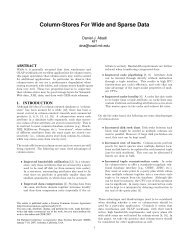
tion about their respective entities in the expected way. Figure 1 

(adapted from Figure 2 of [19]) shows the schema of the tables. 

As with TPC-H, there is a base “scale factor” which can be used 

to scale the size of the benchmark. The sizes of each of the tables 

are defined relative to this scale factor. In this paper, we use a scale 

factor of 10 (yielding a LINEORDER table with 60,000,000 tuples). 

CUSTOMER 

CUSTKEY 

NAME 

ADDRESS 

CITY 

NATION 

REGION 

PHONE 

MKTSEGMENT 

Size=scalefactor x 

30,0000 

SUPPLIER 

SUPPKEY 

NAME 

ADDRESS 

CITY 

NATION 

REGION 

PHONE 


2,000 

LINEORDER 

ORDERKEY 

LINENUMBER 

CUSTKEY 

PARTKEY 

SUPPKEY 

ORDERDATE 

ORDPRIORITY 

SHIPPRIORITY 

QUANTITY 

EXTENDEDPRICE 

ORDTOTALPRICE 

DISCOUNT 

REVENUE 

SUPPLYCOST 

TAX 

COMMITDATE 

SHIPMODE 


6,000,000 

PART 

PARTKEY 

NAME 

MFGR 

CATEGOTY 

BRAND1 

COLOR 

TYPE 

SIZE 

CONTAINER 

Size=200,000 x 

(1 + log2 scalefactor) 

DATE 

DATEKEY 

DATE 

DAYOFWEEK 

MONTH 

YEAR 

YEARMONTHNUM 

YEARMONTH 

DAYNUMWEEK 

…. (9 add!l attributes) 

Size= 365 x 7 

Figure 1: Schema of the SSBM Benchmark 

Queries: The SSBM consists of thirteen queries divided into 

four categories, or “flights”: 

1. Flight 1 contains 3 queries. Queries have a restriction on 1 dimension 

attribute, as well as the DISCOUNT and QUANTITY 

columns of the LINEORDER table. Queries measure the gain 

in revenue (the product of EXTENDEDPRICE and DISCOUNT) 

that would be achieved if various levels of discount were 

eliminated for various order quantities in a given year. The 

LINEORDER selectivities for the three queries are 1.9×10 −2 , 

6.5 × 10 −4 , and 7.5 × 10 −5 , respectively. 

2. Flight 2 contains 3 queries. Queries have a restriction on 

2 dimension attributes and compute the revenue for particular 

product classes in particular regions, grouped by product 

class and year. The LINEORDER selectivities for the three 

queries are 8.0 × 10 −3 , 1.6 × 10 −3 , and 2.0 × 10 −4 , respectively. 

3. Flight 3 consists of 4 queries, with a restriction on 3 dimensions. 

Queries compute the revenue in a particular region 

over a time period, grouped by customer nation, supplier 

nation, and year. The LINEORDER selectivities for the 

four queries are 3.4 × 10 −2 , 1.4 × 10 −3 , 5.5 × 10 −5 , and 

7.6 × 10 −7 respectively. 

4. Flight 4 consists of three queries. Queries restrict on three dimension 

columns, and compute profit (REVENUE - SUPPLY- 

COST) grouped by year, nation, and category for query 1; 

and for queries 2 and 3, region and category. The LINEORDER 

selectivities for the three queries are 1.6×10 −2 , 4.5×10 −3 , 

and 9.1 × 10 −5 , respectively.

4. ROW-ORIENTED EXECUTION 

In this section, we discuss several different techniques that can 

be used to implement a column-database design in a commercial 

row-oriented DBMS (hereafter, System X). We look at three different 

classes of physical design: a fully vertically partitioned design, 

an “index only” design, and a materialized view design. In our 

evaluation, we also compare against a “standard” row-store design 

with one physical table per relation. 

Vertical Partitioning: The most straightforward way to emulate 

a column-store approach in a row-store is to fully vertically partition 

each relation [16]. In a fully vertically partitioned approach, 

some mechanism is needed to connect fields from the same row 

together (column stores typically match up records implicitly by 

storing columns in the same order, but such optimizations are not 

available in a row store). To accomplish this, the simplest approach 

is to add an integer “position” column to every table – this is often 

preferable to using the primary key because primary keys can 

be large and are sometimes composite (as in the case of the lineorder 

table in SSBM). This approach creates one physical table for 

each column in the logical schema, where the ith table has two 

columns, one with values from column i of the logical schema and 

one with the corresponding value in the position column. Queries 

are then rewritten to perform joins on the position attribute when 

fetching multiple columns from the same relation. In our implementation, 

by default, System X chose to use hash joins for this 

purpose, which proved to be expensive. For that reason, we experimented 

with adding clustered indices on the position column of 

every table, and forced System X to use index joins, but this did 

not improve performance – the additional I/Os incurred by index 

accesses made them slower than hash joins. 

Index-only plans: The vertical partitioning approach has two 

problems. First, it requires the position attribute to be stored in every 

column, which wastes space and disk bandwidth. Second, most 

row-stores store a relatively large header on every tuple, which 

further wastes space (column stores typically – or perhaps even 

by definition – store headers in separate columns to avoid these 

overheads). To ameliorate these concerns, the second approach we 

consider uses index-only plans, where base relations are stored using 

a standard, row-oriented design, but an additional unclustered 

B+Tree index is added on every column of every table. Index-only 

plans – which require special support from the database, but are 

implemented by System X – work by building lists of (recordid,value) 

pairs that satisfy predicates on each table, and merging 

these rid-lists in memory when there are multiple predicates on the 

same table. When required fields have no predicates, a list of all 

(record-id,value) pairs from the column can be produced. Such 

plans never access the actual tuples on disk. Though indices still 

explicitly store rids, they do not store duplicate column values, and 

they typically have a lower per-tuple overhead than the vertical partitioning 

approach since tuple headers are not stored in the index. 

One problem with the index-only approach is that if a column 

has no predicate on it, the index-only approach requires the index 

to be scanned to extract the needed values, which can be slower 

than scanning a heap file (as would occur in the vertical partitioning 

approach.) Hence, an optimization to the index-only approach 

is to create indices with composite keys, where the secondary keys 

are from predicate-less columns. For example, consider the query 

SELECT AVG(salary) FROM emp WHERE age>40 – if we 

have a composite index with an (age,salary) key, then we can answer 

this query directly from this index. If we have separate indices 

on (age) and (salary), an index only plan will have to find record-ids 

corresponding to records with satisfying ages and then merge this 

with the complete list of (record-id, salary) pairs extracted from 

4 

the (salary) index, which will be much slower. We use this optimization 

in our implementation by storing the primary key of each 

dimension table as a secondary sort attribute on the indices over the 

attributes of that dimension table. In this way, we can efficiently access 

the primary key values of the dimension that need to be joined 

with the fact table. 

Materialized Views: The third approach we consider uses materialized 

views. In this approach, we create an optimal set of materialized 

views for every query flight in the workload, where the optimal 

view for a given flight has only the columns needed to answer 

queries in that flight. We do not pre-join columns from different 

tables in these views. Our objective with this strategy is to allow 

System X to access just the data it needs from disk, avoiding the 

overheads of explicitly storing record-id or positions, and storing 

tuple headers just once per tuple. Hence, we expect it to perform 

better than the other two approaches, although it does require the 

query workload to be known in advance, making it practical only 

in limited situations. 

5. COLUMN-ORIENTED EXECUTION 

Now that we’ve presented our row-oriented designs, in this section, 

we review three common optimizations used to improve performance 

in column-oriented database systems, and introduce the 

invisible join. 

5.1 Compression 

Compressing data using column-oriented compression algorithms 

and keeping data in this compressed format as it is operated upon 

has been shown to improve query performance by up to an order 

of magnitude [4]. Intuitively, data stored in columns is more 

compressible than data stored in rows. Compression algorithms 

perform better on data with low information entropy (high data 

value locality). Take, for example, a database table containing information 

about customers (name, phone number, e-mail address, 

snail-mail address, etc.). Storing data in columns allows all of the 

names to be stored together, all of the phone numbers together, 

etc. Certainly phone numbers are more similar to each other than 

surrounding text fields like e-mail addresses or names. Further, 

if the data is sorted by one of the columns, that column will be 

super-compressible (for example, runs of the same value can be 

run-length encoded). 

But of course, the above observation only immediately affects 

compression ratio. Disk space is cheap, and is getting cheaper 

rapidly (of course, reducing the number of needed disks will reduce 

power consumption, a cost-factor that is becoming increasingly 

important). However, compression improves performance (in 

addition to reducing disk space) since if data is compressed, then 

less time must be spent in I/O as data is read from disk into memory 

(or from memory to CPU). Consequently, some of the “heavierweight” 

compression schemes that optimize for compression ratio 

(such as Lempel-Ziv, Huffman, or arithmetic encoding), might be 

less suitable than “lighter-weight” schemes that sacrifice compression 

ratio for decompression performance [4, 26]. In fact, compression 

can improve query performance beyond simply saving on 

I/O. If a column-oriented query executor can operate directly on 

compressed data, decompression can be avoided completely and 

performance can be further improved. For example, for schemes 

like run-length encoding – where a sequence of repeated values is 

replaced by a count and the value (e.g., 1, 1, 1, 2, 2 → 1 × 3, 2 × 2) 

– operating directly on compressed data results in the ability of a 

query executor to perform the same operation on multiple column 

values at once, further reducing CPU costs. 

Prior work [4] concludes that the biggest difference between

compression in a row-store and compression in a column-store are 

the cases where a column is sorted (or secondarily sorted) and there 

are consecutive repeats of the same value in a column. In a columnstore, 

it is extremely easy to summarize these value repeats and operate 

directly on this summary. In a row-store, the surrounding data 

from other attributes significantly complicates this process. Thus, 

in general, compression will have a larger impact on query performance 

if a high percentage of the columns accessed by that query 

have some level of order. For the benchmark we use in this paper, 

we do not store multiple copies of the fact table in different sort orders, 

and so only one of the seventeen columns in the fact table can 

be sorted (and two others secondarily sorted) so we expect compression 

to have a somewhat smaller (and more variable per query) 

effect on performance than it could if more aggressive redundancy 

was used. 

5.2 Late Materialization 

In a column-store, information about a logical entity (e.g., a person) 

is stored in multiple locations on disk (e.g. name, e-mail 

address, phone number, etc. are all stored in separate columns), 

whereas in a row store such information is usually co-located in 

a single row of a table. However, most queries access more than 

one attribute from a particular entity. Further, most database output 

standards (e.g., ODBC and JDBC) access database results entity-ata-time 

(not column-at-a-time). Thus, at some point in most query 

plans, data from multiple columns must be combined together into 

‘rows’ of information about an entity. Consequently, this join-like 

materialization of tuples (also called “tuple construction”) is an extremely 

common operation in a column store. 

Naive column-stores [13, 14] store data on disk (or in memory) 

column-by-column, read in (to CPU from disk or memory) only 

those columns relevant for a particular query, construct tuples from 

their component attributes, and execute normal row-store operators 

on these rows to process (e.g., select, aggregate, and join) data. Although 

likely to still outperform the row-stores on data warehouse 

workloads, this method of constructing tuples early in a query plan 

(“early materialization”) leaves much of the performance potential 

of column-oriented databases unrealized. 

More recent column-stores such as X100, C-Store, and to a lesser 

extent, Sybase IQ, choose to keep data in columns until much later 

into the query plan, operating directly on these columns. In order 

to do so, intermediate “position” lists often need to be constructed 

in order to match up operations that have been performed on different 

columns. Take, for example, a query that applies a predicate on 

two columns and projects a third attribute from all tuples that pass 

the predicates. In a column-store that uses late materialization, the 

predicates are applied to the column for each attribute separately 

and a list of positions (ordinal offsets within a column) of values 

that passed the predicates are produced. Depending on the predicate 

selectivity, this list of positions can be represented as a simple 

array, a bit string (where a 1 in the ith bit indicates that the ith 

value passed the predicate) or as a set of ranges of positions. These 

position representations are then intersected (if they are bit-strings, 

bit-wise AND operations can be used) to create a single position 

list. This list is then sent to the third column to extract values at the 

desired positions. 

The advantages of late materialization are four-fold. First, selection 

and aggregation operators tend to render the construction 

of some tuples unnecessary (if the executor waits long enough before 

constructing a tuple, it might be able to avoid constructing it 

altogether). Second, if data is compressed using a column-oriented 

compression method, it must be decompressed before the combination 

of values with values from other columns. This removes 

5 

the advantages of operating directly on compressed data described 

above. Third, cache performance is improved when operating directly 

on column data, since a given cache line is not polluted with 

surrounding irrelevant attributes for a given operation (as shown 

in PAX [6]). Fourth, the block iteration optimization described in 

the next subsection has a higher impact on performance for fixedlength 

attributes. In a row-store, if any attribute in a tuple is variablewidth, 

then the entire tuple is variable width. In a late materialized 

column-store, fixed-width columns can be operated on separately. 

5.3 Block Iteration 

In order to process a series of tuples, row-stores first iterate through 

each tuple, and then need to extract the needed attributes from these 

tuples through a tuple representation interface [11]. In many cases, 

such as in MySQL, this leads to tuple-at-a-time processing, where 

there are 1-2 function calls to extract needed data from a tuple for 

each operation (which if it is a small expression or predicate evaluation 

is low cost compared with the function calls) [25]. 

Recent work has shown that some of the per-tuple overhead of 

tuple processing can be reduced in row-stores if blocks of tuples are 

available at once and operated on in a single operator call [24, 15], 

and this is implemented in IBM DB2 [20]. In contrast to the caseby-case 

implementation in row-stores, in all column-stores (that we 

are aware of), blocks of values from the same column are sent to 

an operator in a single function call. Further, no attribute extraction 

is needed, and if the column is fixed-width, these values can be 

iterated through directly as an array. Operating on data as an array 

not only minimizes per-tuple overhead, but it also exploits potential 

for parallelism on modern CPUs, as loop-pipelining techniques can 

be used [9]. 

5.4 Invisible Join 

Queries over data warehouses, particularly over data warehouses 

modeled with a star schema, often have the following structure: Restrict 

the set of tuples in the fact table using selection predicates on 

one (or many) dimension tables. Then, perform some aggregation 

on the restricted fact table, often grouping by other dimension table 

attributes. Thus, joins between the fact table and dimension tables 

need to be performed for each selection predicate and for each aggregate 

grouping. A good example of this is Query 3.1 from the 

Star Schema Benchmark. 

SELECT c.nation, s.nation, d.year, 

sum(lo.revenue) as revenue 

FROM customer AS c, lineorder AS lo, 

supplier AS s, dwdate AS d 

WHERE lo.custkey = c.custkey 

AND lo.suppkey = s.suppkey 

AND lo.orderdate = d.datekey 

AND c.region = ’ASIA’ 

AND s.region = ’ASIA’ 

AND d.year >= 1992 and d.year

performed first, filtering the lineorder table so that only orders 

from customers who live in Asia remain. As this join is performed, 

the nation of these customers are added to the joined 

customer-order table. These results are pipelined into a join 

with the supplier table where the s.region = ’ASIA’ predicate 

is applied and s.nation extracted, followed by a join with 

the data table and the year predicate applied. The results of these 

joins are then grouped and aggregated and the results sorted according 

to the ORDER BY clause. 

An alternative to the traditional plan is the late materialized join 

technique [5]. In this case, a predicate is applied on the c.region 

column (c.region = ’ASIA’), and the customer key of the 

customer table is extracted at the positions that matched this predicate. 

These keys are then joined with the customer key column 

from the fact table. The results of this join are two sets of positions, 

one for the fact table and one for the dimension table, indicating 

which pairs of tuples from the respective tables passed the 

join predicate and are joined. In general, at most one of these two 

position lists are produced in sorted order (the outer table in the 

join, typically the fact table). Values from the c.nation column 

at this (out-of-order) set of positions are then extracted, along with 

values (using the ordered set of positions) from the other fact table 

columns (supplier key, order date, and revenue). Similar joins are 

then performed with the supplier and date tables. 

Each of these plans have a set of disadvantages. In the first (traditional) 

case, constructing tuples before the join precludes all of 

the late materialization benefits described in Section 5.2. In the 

second case, values from dimension table group-by columns need 

to be extracted in out-of-position order, which can have significant 

cost [5]. 

As an alternative to these query plans, we introduce a technique 

we call the invisible join that can be used in column-oriented databases 

for foreign-key/primary-key joins on star schema style tables. It is 

a late materialized join, but minimizes the values that need to be 

extracted out-of-order, thus alleviating both sets of disadvantages 

described above. It works by rewriting joins into predicates on 

the foreign key columns in the fact table. These predicates can 

be evaluated either by using a hash lookup (in which case a hash 

join is simulated), or by using more advanced methods, such as a 

technique we call between-predicate rewriting, discussed in Section 

5.4.2 below. 

By rewriting the joins as selection predicates on fact table columns, 

they can be executed at the same time as other selection predicates 

that are being applied to the fact table, and any of the predicate 

application algorithms described in previous work [5] can be 

used. For example, each predicate can be applied in parallel and 

the results merged together using fast bitmap operations. Alternatively, 

the results of a predicate application can be pipelined into 

another predicate application to reduce the number of times the 

second predicate must be applied. Only after all predicates have 

been applied are the appropriate tuples extracted from the relevant 

dimensions (this can also be done in parallel). By waiting until 

all predicates have been applied before doing this extraction, the 

number of out-of-order extractions is minimized. 

The invisible join extends previous work on improving performance 

for star schema joins [17, 23] that are reminiscent of semijoins 

[8] by taking advantage of the column-oriented layout, and 

rewriting predicates to avoid hash-lookups, as described below. 

5.4.1 Join Details 

The invisible join performs joins in three phases. First, each 

predicate is applied to the appropriate dimension table to extract a 

list of dimension table keys that satisfy the predicate. These keys 

6 

are used to build a hash table that can be used to test whether a 

particular key value satisfies the predicate (the hash table should 

easily fit in memory since dimension tables are typically small and 

the table contains only keys). An example of the execution of this 

first phase for the above query on some sample data is displayed in 

Figure 2. 

Apply region = 'Asia' on Customer table 

custkey 

1 

region 

nation 

Asia China ... 

2 Europe France ... 

3 Asia India 

Apply region = 'Asia' on Supplier table 

suppkey region nation ... 

1 

2 

dateid 

01011997 

01021997 

01031997 

Asia Russia 

Europe Spain 

Apply year in [1992,1997] on Date table 

year 

1997 

... 

... 

1997 ... 

1997 ... 

... 

... 

... 

... 

Hash table 

with keys 

1 and 3 

Hash table 

with key 1 

Hash table with 

keys 01011997, 

01021997, and 

01031997 

Figure 2: The first phase of the joins needed to execute Query 

3.1 from the Star Schema benchmark on some sample data 

In the next phase, each hash table is used to extract the positions 

of records in the fact table that satisfy the corresponding predicate. 

This is done by probing into the hash table with each value in the 

foreign key column of the fact table, creating a list of all the positions 

in the foreign key column that satisfy the predicate. Then, the 

position lists from all of the predicates are intersected to generate 

a list of satisfying positions P in the fact table. An example of the 

execution of this second phase is displayed in Figure 3. Note that 

a position list may be an explicit list of positions, or a bitmap as 

shown in the example. 

Hash table 

with keys 

1 and 3 

probe 

= 

matching fact 

table bitmap 

for cust. dim. 

join 

Fact Table 

orderkey custkey suppkey orderdate revenue 

1 

3 

1 01011997 43256 

2 3 

2 01011997 33333 

3 2 1 01021997 12121 

4 

1 

1 01021997 23233 

5 2 2 01021997 45456 

6 1 

2 01031997 43251 

7 3 

2 01031997 34235 

1 

1 

0 

1 

0 

1 

1 

probe 

Hash table 

with key 1 

= 

1 

0 

1 

1 

0 

0 

0 

Bitwise 

And 

probe 

Hash table with 

keys 01011997, 

01021997, and 

01031997 

= 

1 

0 

0 

1 

0 

0 

0 

= 

fact table 

tuples that 

satisfy all join 

predicates 

Figure 3: The second phase of the joins needed to execute 

Query 3.1 from the Star Schema benchmark on some sample 

data 

The third phase of the join uses the list of satisfying positions P 

in the fact table. For each column C in the fact table containing a 

foreign key reference to a dimension table that is needed to answer 

1 

1 

1 

1 

1 

1 

1

Fact Table Columns 

custkey 

3 

3 

2 

1 

2 

1 

3 

suppkey 

1 

2 

1 

1 

2 

2 

2 

orderdate 

01011997 

01011997 

01021997 

01021997 

01021997 

01031997 

01031997 

1 

0 

0 

1 

0 

0 

0 

fact table 

tuples that 

satisfy all join 

predicates 

bitmap 

value 

extraction 

bitmap 

value 

extraction 

3 

1 

dateid 

01011997 

01021997 

01031997 

bitmap 01011997 

value = 

01021997 

extraction 

= 

= 

dimension table 

1 

1 

nation 

China 

France 

India 

Positions 

nation 

Russia 

Spain 

Positions 

Values 

position 

lookup 

position 

lookup 

year 

1997 

1997 

1997 

join 

= 

= 

= 

India 

China 

Russia 

Russia 

Figure 4: The third phase of the joins needed to execute Query 

3.1 from the Star Schema benchmark on some sample data 

the query (e.g., where the dimension column is referenced in the 

select list, group by, or aggregate clauses), foreign key values from 

C are extracted using P and are looked up in the corresponding 

dimension table. Note that if the dimension table key is a sorted, 

contiguous list of identifiers starting from 1 (which is the common 

case), then the foreign key actually represents the position of the 

desired tuple in dimension table. This means that the needed dimension 

table columns can be extracted directly using this position 

list (and this is simply a fast array look-up). 

This direct array extraction is the reason (along with the fact that 

dimension tables are typically small so the column being looked 

up can often fit inside the L2 cache) why this join does not suffer 

from the above described pitfalls of previously published late materialized 

join approaches [5] where this final position list extraction 

is very expensive due to the out-of-order nature of the dimension 

table value extraction. Further, the number values that need to be 

extracted is minimized since the number of positions in P is dependent 

on the selectivity of the entire query, instead of the selectivity 

of just the part of the query that has been executed so far. 

An example of the execution of this third phase is displayed in 

Figure 4. Note that for the date table, the key column is not a 

sorted, contiguous list of identifiers starting from 1, so a full join 

must be performed (rather than just a position extraction). Further, 

note that since this is a foreign-key primary-key join, and since all 

predicates have already been applied, there is guaranteed to be one 

and only one result in each dimension table for each position in the 

intersected position list from the fact table. This means that there 

are the same number of results for each dimension table join from 

this third phase, so each join can be done separately and the results 

combined (stitched together) at a later point in the query plan. 

5.4.2 Between-Predicate Rewriting 

As described thus far, this algorithm is not much more than another 

way of thinking about a column-oriented semijoin or a late 

materialized hash join. Even though the hash part of the join is expressed 

as a predicate on a fact table column, practically there is 

little difference between the way the predicate is applied and the 

way a (late materialization) hash join is executed. The advantage 

1997 

1997 

Join Results 

7 

of expressing the join as a predicate comes into play in the surprisingly 

common case (for star schema joins) where the set of keys in 

dimension table that remain after a predicate has been applied are 

contiguous. When this is the case, a technique we call “betweenpredicate 

rewriting” can be used, where the predicate can be rewritten 

from a hash-lookup predicate on the fact table to a “between” 

predicate where the foreign key falls between two ends of the key 

range. For example, if the contiguous set of keys that are valid after 

a predicate has been applied are keys 1000-2000, then instead 

of inserting each of these keys into a hash table and probing the 

hash table for each foreign key value in the fact table, we can simply 

check to see if the foreign key is in between 1000 and 2000. If 

so, then the tuple joins; otherwise it does not. Between-predicates 

are faster to execute for obvious reasons as they can be evaluated 

directly without looking anything up. 

The ability to apply this optimization hinges on the set of these 

valid dimension table keys being contiguous. In many instances, 

this property does not hold. For example, a range predicate on 

a non-sorted field results in non-contiguous result positions. And 

even for predicates on sorted fields, the process of sorting the dimension 

table by that attribute likely reordered the primary keys so 

they are no longer an ordered, contiguous set of identifiers. However, 

the latter concern can be easily alleviated through the use of 

dictionary encoding for the purpose of key reassignment (rather 

than compression). Since the keys are unique, dictionary encoding 

the column results in the dictionary keys being an ordered, contiguous 

list starting from 0. As long as the fact table foreign key 

column is encoded using the same dictionary table, the hash-table 

to between-predicate rewriting can be performed. 

Further, the assertion that the optimization works only on predicates 

on the sorted column of a dimension table is not entirely true. 

In fact, dimension tables in data warehouses often contain sets of 

attributes of increasingly finer granularity. For example, the date 

table in SSBM has a year column, a yearmonth column, and 

the complete date column. If the table is sorted by year, secondarily 

sorted by yearmonth, and tertiarily sorted by the complete 

date, then equality predicates on any of those three columns 

will result in a contiguous set of results (or a range predicate on 

the sorted column). As another example, the supplier table 

has a region column, a nation column, and a city column 

(a region has many nations and a nation has many cities). Again, 

sorting from left-to-right will result in predicates on any of those 

three columns producing a contiguous range output. Data warehouse 

queries often access these columns, due to the OLAP practice 

of rolling-up data in successive queries (tell me profit by region, 

tell me profit by nation, tell me profit by city). Thus, “betweenpredicate 

rewriting” can be used more often than one might initially 

expect, and (as we show in the next section), often yields a 

significant performance gain. 

Note that predicate rewriting does not require changes to the 

query optimizer to detect when this optimization can be used. The 

code that evaluates predicates against the dimension table is capable 

of detecting whether the result set is contiguous. If so, the fact 

table predicate is rewritten at run-time. 

6. EXPERIMENTS 

In this section, we compare the row-oriented approaches to the 

performance of C-Store on the SSBM, with the goal of answering 

four key questions: 

1. How do the different attempts to emulate a column store in a 

row-store compare to the baseline performance of C-Store?

2. Is it possible for an unmodified row-store to obtain the benefits 

of column-oriented design? 

3. Of the specific optimizations proposed for column-stores (compression, 

late materialization, and block processing), which 

are the most significant? 

4. How does the cost of performing star schema joins in columnstores 

using the invisible join technique compare with executing 

queries on a denormalized fact table where the join 

has been pre-executed? 

By answering these questions, we provide database implementers 

who are interested in adopting a column-oriented approach with 

guidelines for which performance optimizations will be most fruitful. 

Further, the answers will help us understand what changes need 

to be made at the storage-manager and query executor levels to rowstores 

if row-stores are to successfully simulate column-stores. 

All of our experiments were run on a 2.8 GHz single processor, 

dual core Pentium(R) D workstation with 3 GB of RAM running 

RedHat Enterprise Linux 5. The machine has a 4-disk array, managed 

as a single logical volume with files striped across it. Typical 

I/O throughput is 40 - 50 MB/sec/disk, or 160 - 200 MB/sec in aggregate 

for striped files. The numbers we report are the average of 

several runs, and are based on a “warm” buffer pool (in practice, we 

found that this yielded about a 30% performance increase for both 

systems; the gain is not particularly dramatic because the amount 

of data read by each query exceeds the size of the buffer pool). 

6.1 Motivation for Experimental Setup 

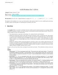
Figure 5 compares the performance of C-Store and System X on 

the Star Schema Benchmark. We caution the reader to not read 

too much into absolute performance differences between the two 

systems — as we discuss in this section, there are substantial differences 

in the implementations of these systems beyond the basic 

difference of rows vs. columns that affect these performance numbers. 

In this figure, “RS” refers to numbers for the base System X case, 

“CS” refers to numbers for the base C-Store case, and “RS (MV)” 

refers to numbers on System X using an optimal collection of materialized 

views containing minimal projections of tables needed to 

answer each query (see Section 4). As shown, C-Store outperforms 

System X by a factor of six in the base case, and a factor of three 

when System X is using materialized views. This is consistent with 

previous work that shows that column-stores can significantly outperform 

row-stores on data warehouse workloads [2, 9, 22]. 

However, the fourth set of numbers presented in Figure 5, “CS 

(Row-MV)” illustrate the caution that needs to be taken when comparing 

numbers across systems. For these numbers, we stored the 

identical (row-oriented!) materialized view data inside C-Store. 

One might expect the C-Store storage manager to be unable to store 

data in rows since, after all, it is a column-store. However, this can 

be done easily by using tables that have a single column of type 

“string”. The values in this column are entire tuples. One might 

also expect that the C-Store query executer would be unable to operate 

on rows, since it expects individual columns as input. However, 

rows are a legal intermediate representation in C-Store — as 

explained in Section 5.2, at some point in a query plan, C-Store reconstructs 

rows from component columns (since the user interface 

to a RDBMS is row-by-row). After it performs this tuple reconstruction, 

it proceeds to execute the rest of the query plan using 

standard row-store operators [5]. Thus, both the “CS (Row-MV)” 

and the “RS (MV)” are executing the same queries on the same input 

data stored in the same way. Consequently, one might expect 

these numbers to be identical. 

8 

In contrast with this expectation, the System X numbers are significantly 

faster (more than a factor of two) than the C-Store numbers. 

In retrospect, this is not all that surprising — System X has 

teams of people dedicated to seeking and removing performance 

bottlenecks in the code, while C-Store has multiple known performance 

bottlenecks that have yet to be resolved [3]. Moreover, C- 

Store, as a simple prototype, has not implemented advanced performance 

features that are available in System X. Two of these features 

are partitioning and multi-threading. System X is able to partition 

each materialized view optimally for the query flight that it is designed 

for. Partitioning improves performance when running on a 

single machine by reducing the data that needs to be scanned in order 

to answer a query. For example, the materialized view used for 

query flight 1 is partitioned on orderdate year, which is useful since 

each query in this flight has a predicate on orderdate. To determine 

the performance advantage System X receives from partitioning, 

we ran the same benchmark on the same materialized views without 

partitioning them. We found that the average query time in this 

case was 20.25 seconds. Thus, partitioning gives System X a factor 

of two advantage (though this varied by query, which will be 

discussed further in Section 6.2). C-Store is also at a disadvantage 

since it not multi-threaded, and consequently is unable to take 

advantage of the extra core. 

Thus, there are many differences between the two systems we experiment 

with in this paper. Some are fundamental differences between 

column-stores and row-stores, and some are implementation 

artifacts. Since it is difficult to come to useful conclusions when 

comparing numbers across different systems, we choose a different 

tactic in our experimental setup, exploring benchmark performance 

from two angles. In Section 6.2 we attempt to simulate a columnstore 

inside of a row-store. The experiments in this section are only 

on System X, and thus we do not run into cross-system comparison 

problems. In Section 6.3, we remove performance optimizations 

from C-Store until row-store performance is achieved. Again, all 

experiments are on only a single system (C-Store). 

By performing our experiments in this way, we are able to come 

to some conclusions about the performance advantage of columnstores 

without relying on cross-system comparisons. For example, 

it is interesting to note in Figure 5 that there is more than a factor 

of six difference between “CS” and “CS (Row MV)” despite the 

fact that they are run on the same system and both read the minimal 

set of columns off disk needed to answer each query. Clearly the 

performance advantage of a column-store is more than just the I/O 

advantage of reading in less data from disk. We will explain the 

reason for this performance difference in Section 6.3. 

6.2 Column-Store Simulation in a Row-Store 

In this section, we describe the performance of the different configurations 

of System X on the Star Schema Benchmark. We configured 

System X to partition the lineorder table on orderdate 

by year (this means that a different physical partition is created 

for tuples from each year in the database). As described in 

Section 6.1, this partitioning substantially speeds up SSBM queries 

that involve a predicate on orderdate (queries 1.1, 1.2, 1.3, 3.4, 

4.2, and 4.3 query just 1 year; queries 3.1, 3.2, and 3.3 include a 

substantially less selective query over half of years). Unfortunately, 

for the column-oriented representations, System X doesn’t allow us 

to partition two-column vertical partitions on orderdate (since 

they do not contain the orderdate column, except, of course, 

for the orderdate vertical partition), which means that for those 

query flights that restrict on the orderdate column, the columnoriented 

approaches are at a disadvantage relative to the base case. 

Nevertheless, we decided to use partitioning for the base case

Time (seconds) 

60 

40 

20 

0 

1.1 1.2 1.3 2.1 2.2 2.3 3.1 3.2 3.3 3.4 4.1 4.2 4.3 AVG 

RS 2.7 2.0 1.5 43.8 44.1 46.0 43.0 42.8 31.2 6.5 44.4 14.1 12.2 25.7 

RS (MV) 1.0 1.0 0.2 15.5 13.5 11.8 16.1 6.9 6.4 3.0 29.2 22.4 6.4 10.2 

CS 0.4 0.1 0.1 5.7 4.2 3.9 11.0 4.4 7.6 0.6 8.2 3.7 2.6 4.0 

CS (Row-MV) 16.0 9.1 8.4 33.5 23.5 22.3 48.5 21.5 17.6 17.4 48.6 38.4 32.1 25.9 

Figure 5: Baseline performance of C-Store “CS” and System X “RS”, compared with materialized view cases on the same systems. 

because it is in fact the strategy that a database administrator would 

use when trying to improve the performance of these queries on a 

row-store. When we ran the base case without partitioning, performance 

was reduced by a factor of two on average (though this 

varied per query depending on the selectivity of the predicate on 

the orderdate column). Thus, we would expect the vertical 

partitioning case to improve by a factor of two, on average, if it 

were possible to partition tables based on two levels of indirection 

(from primary key, or record-id, we get orderdate, and 

from orderdate we get year). 

Other relevant configuration parameters for System X include: 

32 KB disk pages, a 1.5 GB maximum memory for sorts, joins, 

intermediate results, and a 500 MB buffer pool. We experimented 

with different buffer pool sizes and found that different sizes did 

not yield large differences in query times (due to dominant use of 

large table scans in this benchmark), unless a very small buffer pool 

was used. We enabled compression and sequential scan prefetching, 

and we noticed that both of these techniques improved performance, 

again due to the large amount of I/O needed to process 

these queries. System X also implements a star join and the optimizer 

will use bloom filters when it expects this will improve query 

performance. 

Recall from Section 4 that we experimented with six configurations 

of System X on SSBM: 

1. A “traditional” row-oriented representation; here, we allow 

System X to use bitmaps and bloom filters if they are beneficial. 

2. A “traditional (bitmap)” approach, similar to traditional, but 

with plans biased to use bitmaps, sometimes causing them to 

produce inferior plans to the pure traditional approach. 

3. A “vertical partitioning” approach, with each column in its 

own relation with the record-id from the original relation. 

4. An “index-only” representation, using an unclustered B+tree 

on each column in the row-oriented approach, and then answering 

queries by reading values directly from the indexes. 

5. A “materialized views” approach with the optimal collection 

of materialized views for every query (no joins were performed 

in advance in these views). 

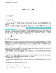
The detailed results broken down by query flight are shown in 

Figure 6(a), with average results across all queries shown in Fig- 

9 

ure 6(b). Materialized views perform best in all cases, because they 

read the minimal amount of data required to process a query. After 

materialized views, the traditional approach or the traditional 

approach with bitmap indexing, is usually the best choice. On 

average, the traditional approach is about three times better than 

the best of our attempts to emulate a column-oriented approach. 

This is particularly true of queries that can exploit partitioning on 

orderdate, as discussed above. For query flight 2 (which does 

not benefit from partitioning), the vertical partitioning approach is 

competitive with the traditional approach; the index-only approach 

performs poorly for reasons we discuss below. Before looking at 

the performance of individual queries in more detail, we summarize 

the two high level issues that limit the approach of the columnar approaches: 

tuple overheads, and inefficient tuple reconstruction: 

Tuple overheads: As others have observed [16], one of the problems 

with a fully vertically partitioned approach in a row-store is 

that tuple overheads can be quite large. This is further aggravated 

by the requirement that record-ids or primary keys be stored with 

each column to allow tuples to be reconstructed. We compared 

the sizes of column-tables in our vertical partitioning approach to 

the sizes of the traditional row store tables, and found that a single 

column-table from our SSBM scale 10 lineorder table (with 60 

million tuples) requires between 0.7 and 1.1 GBytes of data after 

compression to store – this represents about 8 bytes of overhead 

per row, plus about 4 bytes each for the record-id and the column 

attribute, depending on the column and the extent to which compression 

is effective (16 bytes × 6 × 10 7 tuples = 960 MB). In 

contrast, the entire 17 column lineorder table in the traditional 

approach occupies about 6 GBytes decompressed, or 4 GBytes 

compressed, meaning that scanning just four of the columns in the 

vertical partitioning approach will take as long as scanning the entire 

fact table in the traditional approach. As a point of comparison, 

in C-Store, a single column of integers takes just 240 MB 

(4 bytes × 6 × 10 7 tuples = 240 MB), and the entire table compressed 

takes 2.3 Gbytes. 

Column Joins: As we mentioned above, merging two columns 

from the same table together requires a join operation. System 

X favors using hash-joins for these operations. We experimented 

with forcing System X to use index nested loops and merge joins, 

but found that this did not improve performance because index accesses 

had high overhead and System X was unable to skip the sort 

preceding the merge join.



120.0 

100.0 

80.0 

60.0 

40.0 

20.0 

0.0 

Flight 1 

T T(B) MV VP AI 

Q1.1 2.7 9.9 1.0 69.7 107.2 

Q1.2 2.0 11.0 1.0 36.0 50.8 

Q1.3 1.5 1.5 0.2 36.0 48.5 

600.0 

500.0 

400.0 

300.0 

200.0 

100.0 

0.0 

Flight 3 


Q3.1 43.0 91.4 16.1 139.1 413.8 

Q3.2 42.8 65.3 6.9 63.9 40.7 

Q3.3 31.2 31.2 6.4 48.2 531.4 

Q3.4 6.5 6.5 3.0 47.0 65.5 

400.0 

350.0 

300.0 

250.0 

200.0 

150.0 

100.0 

50.0 

0.0 

Flight 2 


Q2.1 43.8 91.9 15.5 65.1 359.8 

Q2.2 44.1 78.4 13.5 48.8 46.4 

Q2.3 46.0 304.1 11.8 39.0 43.9 

700.0 

600.0 

500.0 

400.0 

300.0 

200.0 

100.0 

0.0 

Flight 4 


Q4.1 44.4 94.4 29.2 208.6 623.9 

Q4.2 14.1 25.3 22.4 150.4 280.1 

Q4.3 12.2 21.2 6.4 86.3 263.9 


250.0 

200.0 

150.0 

100.0 

50.0 

0.0 

Average 


Average 25.7 64.0 10.2 79.9 221.2 

(a) (b) 

Figure 6: (a) Performance numbers for different variants of the row-store by query flight. Here, T is traditional, T(B) is traditional 

(bitmap), MV is materialized views, VP is vertical partitioning, and AI is all indexes. (b) Average performance across all queries. 

6.2.1 Detailed Row-store Performance Breakdown 

In this section, we look at the performance of the row-store approaches, 

using the plans generated by System X for query 2.1 from 

the SSBM as a guide (we chose this query because it is one of the 

few that does not benefit from orderdate partitioning, so provides 

a more equal comparison between the traditional and vertical 

partitioning approach.) Though we do not dissect plans for other 

queries as carefully, their basic structure is the same. The SQL for 

this query is: 

SELECT sum(lo.revenue), d.year, p.brand1 

FROM lineorder AS lo, dwdate AS d, 

part AS p, supplier AS s 

WHERE lo.orderdate = d.datekey 

AND lo.partkey = p.partkey 

AND lo.suppkey = s.suppkey 

AND p.category = ’MFGR#12’ 

AND s.region = ’AMERICA’ 

GROUP BY d.year, p.brand1 

ORDER BY d.year, p.brand1 

The selectivity of this query is 8.0 × 10 −3 . Here, the vertical partitioning 

approach performs about as well as the traditional approach 

(65 seconds versus 43 seconds), but the index-only approach performs 

substantially worse (360 seconds). We look at the reasons 

for this below. 

Traditional: For this query, the traditional approach scans the entire 

lineorder table, using hash joins to join it with the dwdate, 

part, and supplier table (in that order). It then performs a sortbased 

aggregate to compute the final answer. The cost is dominated 

by the time to scan the lineorder table, which in our system requires 

about 40 seconds. Materialized views take just 15 seconds, 

because they have to read about 1/3rd of the data as the traditional 

approach. 

Vertical partitioning: The vertical partitioning approach hashjoins 

the partkey column with the filtered part table, and the 

10 

suppkey column with the filtered supplier table, and then 

hash-joins these two result sets. This yields tuples with the recordid 

from the fact table and the p.brand1 attribute of the part 

table that satisfy the query. System X then hash joins this with the 

dwdate table to pick up d.year, and finally uses an additional 

hash join to pick up the lo.revenue column from its column table. 

This approach requires four columns of the lineorder table 

to be read in their entirety (sequentially), which, as we said above, 

requires about as many bytes to be read from disk as the traditional 

approach, and this scan cost dominates the runtime of this query, 

yielding comparable performance as compared to the traditional 

approach. Hash joins in this case slow down performance by about 

25%; we experimented with eliminating the hash joins by adding 

clustered B+trees on the key columns in each vertical partition, but 

System X still chose to use hash joins in this case. 

Index-only plans: Index-only plans access all columns through 

unclustered B+Tree indexes, joining columns from the same table 

on record-id (so they never follow pointers back to the base 

relation). The plan for query 2.1 does a full index scan on the 

suppkey, revenue, partkey, and orderdate columns of 

the fact table, joining them in that order with hash joins. In this 

case, the index scans are relatively fast sequential scans of the entire 

index file, and do not require seeks between leaf pages. The 

hash joins, however, are quite slow, as they combine two 60 million 

tuple columns each of which occupies hundreds of megabytes 

of space. Note that hash join is probably the best option for these 

joins, as the output of the index scans is not sorted on record-id, and 

sorting record-id lists or performing index-nested loops is likely to 

be much slower. As we discuss below, we couldn’t find a way to 

force System X to defer these joins until later in the plan, which 

would have made the performance of this approach closer to vertical 

partitioning. 

After joining the columns of the fact table, the plan uses an index 

range scan to extract the filtered part.category column and 

hash joins it with the part.brand1 column and the part.part-

key column (both accessed via full index scans). It then hash 

joins this result with the already joined columns of the fact table. 

Next, it hash joins supplier.region (filtered through an index 

range scan) and the supplier.suppkey columns (accessed 

via full index scan), and hash joins that with the fact table. Finally, 

it uses full index scans to access the dwdate.datekey 

and dwdate.year columns, joins them using hash join, and hash 

joins the result with the fact table. 

6.2.2 Discussion 

The previous results show that none of our attempts to emulate a 

column-store in a row-store are particularly effective. The vertical 

partitioning approach can provide performance that is competitive 

with or slightly better than a row-store when selecting just a few 

columns. When selecting more than about 1/4 of the columns, however, 

the wasted space due to tuple headers and redundant copies of 

the record-id yield inferior performance to the traditional approach. 

This approach also requires relatively expensive hash joins to combine 

columns from the fact table together. It is possible that System 

X could be tricked into storing the columns on disk in sorted order 

and then using a merge join (without a sort) to combine columns 

from the fact table but our DBA was unable to coax this behavior 

from the system. 

Index-only plans have a lower per-record overhead, but introduce 

another problem – namely, the system is forced to join columns of 

the fact table together using expensive hash joins before filtering 

the fact table using dimension columns. It appears that System X is 

unable to defer these joins until later in the plan (as the vertical partitioning 

approach does) because it cannot retain record-ids from 

the fact table after it has joined with another table. These giant 

hash joins lead to extremely slow performance. 

With respect to the traditional plans, materialized views are an 

obvious win as they allow System X to read just the subset of 

the fact table that is relevant, without merging columns together. 

Bitmap indices sometimes help – especially when the selectivity 

of queries is low – because they allow the system to skip over 

some pages of the fact table when scanning it. In other cases, they 

slow the system down as merging bitmaps adds some overhead to 

plan execution and bitmap scans can be slower than pure sequential 

scans. 

As a final note, we observe that implementing these plans in System 

X was quite painful. We were required to rewrite all of our 

queries to use the vertical partitioning approaches, and had to make 

extensive use of optimizer hints and other trickery to coax the system 

into doing what we desired. 

In the next section we study how a column-store system designed 

from the ground up is able to circumvent these limitations, and 

break down the performance advantages of the different features 

of the C-Store system on the SSBM benchmark. 

6.3 Column-Store Performance 

It is immediately apparent upon the inspection of the average 

query time in C-Store on the SSBM (around 4 seconds) that it is 

faster than not only the simulated column-oriented stores in the 

row-store (80 seconds to 220 seconds), but even faster than the 

best-case scenario for the row-store where the queries are known in 

advance and the row-store has created materialized views tailored 

for the query plans (10.2 seconds). Part of this performance difference 

can be immediately explained without further experiments 

– column-stores do not suffer from the tuple overhead and high 

column join costs that row-stores do (this will be explained in Section 

6.3.1). However, this observation does not explain the reason 

why the column-store is faster than the materialized view case or 

11 

the “CS Row-MV” case from Section 6.1, where the amount of 

I/O across systems is similar, and the other systems does not need 

join together columns from the same table. In order to understand 

this latter performance difference, we perform additional experiments 

in the column-store where we successively remove columnoriented 

optimizations until the column-store begins to simulate a 

row-store. In so doing, we learn the impact of these various optimizations 

on query performance. These results are presented in 

Section 6.3.2. 

6.3.1 Tuple Overhead and Join Costs 

Modern column-stores do not explicitly store the record-id (or 

primary key) needed to join together columns from the same table. 

Rather, they use implicit column positions to reconstruct columns 

(the ith value from each column belongs to the ith tuple in the table). 

Further, tuple headers are stored in their own separate columns 

and so they can be accessed separately from the actual column values. 

Consequently, a column in a column-store contains just data 

from that column, rather than a tuple header, a record-id, and column 

data in a vertically partitioned row-store. 

In a column-store, heap files are stored in position order (the 

ith value is always after the i − 1st value), whereas the order of 

heap files in many row-stores, even on a clustered attribute, is only 

guaranteed through an index. This makes a merge join (without 

a sort) the obvious choice for tuple reconstruction in a columnstore. 

In a row-store, since iterating through a sorted file must be 

done indirectly through the index, which can result in extra seeks 

between index leaves, an index-based merge join is a slow way to 

reconstruct tuples. 

It should be noted that neither of the above differences between 

column-store performance and row-store performance are fundamental. 

There is no reason why a row-store cannot store tuple 

headers separately, use virtual record-ids to join data, and maintain 

heap files in guaranteed position order. The above observation 

simply highlights some important design considerations that would 

be relevant if one wanted to build a row-store that can successfully 

simulate a column-store. 

6.3.2 Breakdown of Column-Store Advantages 

As described in Section 5, three column-oriented optimizations, 

presented separately in the literature, all claim to significantly improve 

the performance of column-oriented databases. These optimizations 

are compression, late materialization, and block-iteration. 

Further, we extended C-Store with the invisible join technique which 

we also expect will improve performance. Presumably, these optimizations 

are the reason for the performance difference between 

the column-store and the row-oriented materialized view cases from 

Figure 5 (both in System X and in C-Store) that have similar I/O 

patterns as the column-store. In order to verify this presumption, 

we successively removed these optimizations from C-Store and 

measured performance after each step. 

Removing compression from C-Store was simple since C-Store 

includes a runtime flag for doing so. Removing the invisible join 

was also simple since it was a new operator we added ourselves. 

In order to remove late materialization, we had to hand code query 

plans to construct tuples at the beginning of the query plan. Removing 

block-iteration was somewhat more difficult than the other three 

optimizations. C-Store “blocks” of data can be accessed through 

two interfaces: “getNext” and “asArray”. The former method requires 

one function call per value iterated through, while the latter 

method returns a pointer to an array than can be iterated through directly. 

For the operators used in the SSBM query plans that access 

blocks through the “asArray” interface, we wrote alternative ver-



40.0 

35.0 

30.0 

25.0 

20.0 

15.0 

10.0 

5.0 

0.0 

Flight 1 

tICL TICL tiCL TiCL ticL TicL Ticl 

1.1 0.4 0.4 0.3 0.4 3.8 7.1 33.4 

1.2 0.1 0.1 0.1 0.1 2.1 6.1 28.2 

1.3 0.1 0.1 0.1 0.1 2.1 6.0 27.4 

60.0 

50.0 

40.0 

30.0 

20.0 

10.0 

0.0 

Flight 3 


3.1 11.0 17.3 16.0 21.4 31.9 31.9 56.5 

3.2 4.4 11.2 9.0 14.1 15.5 15.5 34.0 

3.3 7.6 12.6 7.5 12.6 13.5 13.6 30.3 

3.4 0.6 0.7 0.6 0.7 13.5 13.6 30.2 

45.0 

40.0 

35.0 

30.0 

25.0 

20.0 

15.0 

10.0 

5.0 

0.0 

Flight 2 


2.1 5.7 7.4 13.6 14.8 15.0 16.1 40.5 

2.2 4.2 6.7 12.6 13.8 13.9 14.9 36.0 

2.3 3.9 6.5 12.2 13.4 13.6 14.7 35.0 

70.0 

60.0 

50.0 

40.0 

30.0 

20.0 

10.0 

0.0 

Flight 4 


4.1 8.2 10.7 15.8 17.0 30.1 30.0 66.3 

4.2 3.7 5.5 5.5 6.9 20.4 21.4 60.8 

4.3 2.6 4.3 4.1 5.4 15.8 16.9 54.4 


45.0 

40.0 

35.0 

30.0 

25.0 

20.0 

15.0 

10.0 

5.0 

0.0 

Average 


Average 4.0 6.4 7.5 9.3 14.7 16.0 41.0 

(a) (b) 

Figure 7: (a) Performance numbers for C-Store by query flight with various optimizations removed. The four letter code indicates 

the C-Store configuration: T=tuple-at-a-time processing, t=block processing; I=invisible join enabled, i=disabled; C=compression 

enabled, c=disabled; L=late materialization enabled, l=disabled. (b) Average performance numbers for C-Store across all queries. 

sions that use “getNext”. We only noticed a significant difference 

in the performance of selection operations using this method. 

Figure 7(a) shows detailed, per-query results of successively removing 

these optimizations from C-Store, with averages across all 

SSBM queries shown in Figure 7(b). Block-processing can improve 

performance anywhere from a factor of only 5% to 50% depending 

on whether compression has already been removed (when 

compression is removed, the CPU benefits of block processing is 

not as significant since I/O becomes a factor). In other systems, 

such as MonetDB/X100, that are more carefully optimized for blockprocessing 

[9], one might expect to see a larger performance degradation 

if this optimization were removed. 

The invisible join improves performance by 50-75%. Since C- 

Store uses the similar “late-materialized join” technique in the absence 

of the invisible join, this performance difference is largely 

due to the between-predicate rewriting optimization. There are 

many cases in the SSBM where the between-predicate rewriting optimization 

can be used. In the supplier table, the region, nation, and 

city columns are attributes of increasingly finer granularity, which, 

as described in Section 5.4, result in contiguous positional result 

sets from equality predicate application on any of these columns. 

The customer table has a similar region, nation, and city column 

trio. The part table has mfgr, category, and brand as attributes of increasingly 

finer granularity. Finally, the date table has year, month, 

and day increasing in granularity. Every query in the SSBM contain 

one or more joins (all but the first query flight contains more 

than one join), and for each query, at least one of the joins is with 

a dimension table that had a predicate on one of these special types 

of attributes. Hence, it was possible to use the between-predicate 

rewriting optimization at least once per query. 

Clearly, the most significant two optimizations are compression 

and late materialization. Compression improves performance by 

almost a factor of two on average. However, as mentioned in Section 

5, we do not redundantly store the fact table in multiple sort 

12 

orders to get the full advantage of compression (only one column – 

the orderdate column – is sorted, and two others secondarily sorted 

– the quantity and discount columns). The columns in the fact table 

that are accessed by the SSBM queries are not very compressible 

if they do not have order to them, since they are either keys 

(which have high cardinality) or are random values. The first query 

flight, which accesses each of the three columns that have order to 

them, demonstrates the performance benefits of compression when 

queries access highly compressible data. In this case, compression 

results in an order of magnitude performance improvement. This 

is because runs of values in the three ordered columns can be runlength 

encoded (RLE). Not only does run-length encoding yield a 

good compression ratio and thus reduced I/O overhead, but RLE is 

also very simple to operate on directly (for example, a predicate or 

an aggregation can be applied to an entire run at once). The primary 

sort column, orderdate, only contains 2405 unique values, and so 

the average run-length for this column is almost 25,000. This column 

takes up less than 64K of space. 

The other significant optimization is late materialization. This 

optimization was removed last since data needs to be decompressed 

in the tuple construction process, and early materialization results 

in row-oriented execution which precludes invisible joins. Late 

materialization results in almost a factor of three performance improvement. 

This is primarily because of the selective predicates in 

some of the SSBM queries. The more selective the predicate, the 

more wasteful it is to construct tuples at the start of a query plan, 

since such are tuples immediately discarded. 

Note that once all of these optimizations are removed, the columnstore 

acts like a row-store. Columns are immediately stitched together 

and after this is done, processing is identical to a row-store. 

Since this is the case, one would expect the column-store to perform 

similarly to the row-oriented materialized view cases from 

Figure 5 (both in System X and in C-Store) since the I/O requirements 

and the query processing are similar – the only difference


50 

40 

30 

20 

10 

0 

1.1 1.2 1.3 2.1 2.2 2.3 3.1 3.2 3.3 3.4 4.1 4.2 4.3 AVG 

Base 0.4 0.1 0.1 5.7 4.2 3.9 11.0 4.4 7.6 0.6 8.2 3.7 2.6 4.0 

PJ, No C 0.4 0.1 0.2 32.9 25.4 12.1 42.7 43.1 31.6 28.4 46.8 9.3 6.8 21.5 

PJ, Int C 0.3 0.1 0.1 11.8 3.0 2.6 11.7 8.3 5.5 4.1 10.0 2.2 1.5 4.7 

PJ, Max C 0.7 0.2 0.2 6.1 2.3 1.9 7.3 3.6 3.9 3.2 6.8 1.8 1.1 3.0 

Figure 8: Comparison of performance of baseline C-Store on the original SSBM schema with a denormalized version of the schema. 

Denormalized columns are either not compressed (“PJ, No C”), dictionary compressed into integers (“PJ, Int C”), or compressed as 

much as possible (“PJ, Max C”). 

is the necessary tuple-construction at the beginning of the query 

plans for the column store. Section 6.1 cautioned against direct 

comparisons with System X, but by comparing these numbers with 

the “CS Row-MV” case from Figure 5, we see how expensive tuple 

construction can be (it adds almost a factor of 2). This is consistent 

with previous results [5]. 

6.3.3 Implications of Join Performance 

In profiling the code, we noticed that in the baseline C-Store 

case, performance is dominated in the lower parts of the query plan 

(predicate application) and that the invisible join technique made 

join performance relatively cheap. In order to explore this observation 

further we created a denormalized version of the fact table 

where the fact table and its dimension table are pre-joined such 

that instead of containing a foreign key into the dimension table, 

the fact table contains all of the values found in the dimension table 

repeated for each fact table record (e.g., all customer information 

is contained in each fact table tuple corresponding to a purchase 

made by that customer). Clearly, this complete denormalization 

would be more detrimental from a performance perspective in a 

row-store since this would significantly widen the table. However, 

in a column-store, one might think this would speed up read-only 

queries since only those columns relevant for a query need to read 

in, and joins would be avoided. 

Surprisingly, we found this often not to be the case. Figure 8 

compares the baseline C-Store performance from the previous section 

(using the invisible join) with the performance of C-Store on 

the same benchmark using three versions of the single denormalized 

table where joins have been performed in advance. In the first 

case, complete strings like customer region and customer nation 

are included unmodified in the denormalized table. This case performs 

a factor of 5 worse than the base case. This is because the 

invisible join converts predicates on dimension table attributes into 

predicates on fact table foreign key values. When the table is denormalized, 

predicate application is performed on the actual string 

attribute in the fact table. In both cases, this predicate application is 

the dominant step. However, a predicate on the integer foreign key 

can be performed faster than a predicate on a string attribute since 

the integer attribute is smaller. 

Of course, the string attributes could have easily been dictionary 

encoded into integers before denormalization. When we did 

13 

this (the “PJ, Int C” case in Figure 8), the performance difference 

between the baseline and the denormalized cases became much 

smaller. Nonetheless, for quite a few queries, the baseline case 

still performed faster. The reasons for this are twofold. First, some 

SSBM queries have two predicates on the same dimension table. 

The invisible join technique is able to summarize the result of this 

double predicate application as a single predicate on the foreign key 

attribute in the fact table. However, for the denormalized case, the 

predicate must be completely applied to both columns in the fact 

table (remember that for data warehouses, fact tables are generally 

much larger than dimension tables, so predicate applications on the 

fact table are much more expensive than predicate applications on 

the dimension tables). 

Second, many queries have a predicate on one attribute in a dimension 

table and group by a different attribute from the same dimension 

table. For the invisible join, this requires iteration through 

the foreign key column once to apply the predicate, and again (after 

all predicates from all tables have been applied and intersected) 

to extract the group-by attribute. But since C-Store uses pipelined 

execution, blocks from the foreign key column will still be in memory 

upon the second access. In the denormalized case, the predicate 

column and the group-by column are separate columns in the fact 

table and both must be iterated through, doubling the necessary I/O. 

In fact, many of the SSBM dimension table columns that are accessed 

in the queries have low cardinality, and can be compressed 

into values that are smaller than the integer foreign keys. When 

using complete C-Store compression, we found that the denormalization 

technique was useful more often (shown as the “PJ, Max C” 

case in Figure 8). 

These results have interesting implications. Denormalization has 

long been used as a technique in database systems to improve query 

performance, by reducing the number of joins that must be performed 

at query time. In general, the school of wisdom teaches 

that denormalization trades query performance for making a table 

wider, and more redundant (increasing the size of the table on disk 

and increasing the risk of update anomalies). One might expect 

that this tradeoff would be more favorable in column-stores (denormalization 

should be used more often) since one of the disadvantages 

of denormalization (making the table wider) is not problematic 

when using a column-oriented layout. However, these results 

show the exact opposite: denormalization is actually not very use-

ful in column-stores (at least for star schemas). This is because the 

invisible join performs so well that reducing the number of joins 

via denormalization provides an insignificant benefit. In fact, denormalization 

only appears to be useful when the dimension table 

attributes included in the fact table are sorted (or secondarily 

sorted) or are otherwise highly compressible. 

7. CONCLUSION 

In this paper, we compared the performance of C-Store to several 

variants of a commercial row-store system on the data warehousing 

benchmark, SSBM. We showed that attempts to emulate the 

physical layout of a column-store in a row-store via techniques like 

vertical partitioning and index-only plans do not yield good performance. 

We attribute this slowness to high tuple reconstruction 

costs, as well as the high per-tuple overheads in narrow, vertically 

partitioned tables. We broke down the reasons why a column-store 

is able to process column-oriented data so effectively, finding that 

late materialization improves performance by a factor of three, and 

that compression provides about a factor of two on average, or an 

order-of-magnitude on queries that access sorted data. We also proposed 

a new join technique, called invisible joins, that further improves 

performance by about 50%. 

The conclusion of this work is not that simulating a columnstore 

in a row-store is impossible. Rather, it is that this simulation 

performs poorly on today’s row-store systems (our experiments 

were performed on a very recent product release of System 

X). A successful column-oriented simulation will require some important 

system improvements, such as virtual record-ids, reduced 

tuple overhead, fast merge joins of sorted data, run-length encoding 

across multiple tuples, and some column-oriented query execution 

techniques like operating directly on compressed data, block processing, 

invisible joins, and late materialization. Some of these improvements 

have been implemented or proposed to be implemented 

in various different row-stores [12, 13, 20, 24]; however, building a 

complete row-store that can transform into a column-store on workloads 

where column-stores perform well is an interesting research 

problem to pursue. 

8. ACKNOWLEDGMENTS 

We thank Stavros Harizopoulos for his comments on this paper, 

and the NSF for funding this research, under grants 0704424 and 

0325525. 

9. REPEATABILITY ASSESSMENT 

All figures containing numbers derived from experiments on the 

C-Store prototype (Figure 7a, Figure 7b, and Figure 8) have been 

verified by the SIGMOD repeatability committee. We thank Ioana 

Manolescu and the repeatability committee for their feedback. 

10. REFERENCES 

[1] http://www.sybase.com/products/ 

informationmanagement/sybaseiq. 

[2] TPC-H Result Highlights Scale 1000GB. 

http://www.tpc.org/tpch/results/ 

tpch result detail.asp?id=107102903. 

[3] D. J. Abadi. Query execution in column-oriented database 

systems. MIT PhD Dissertation, 2008. PhD Thesis. 

[4] D. J. Abadi, S. R. Madden, and M. Ferreira. Integrating 

compression and execution in column-oriented database 

systems. In SIGMOD, pages 671–682, 2006. 

14 

[5] D. J. Abadi, D. S. Myers, D. J. DeWitt, and S. R. Madden. 

Materialization strategies in a column-oriented DBMS. In 

ICDE, pages 466–475, 2007. 

[6] A. Ailamaki, D. J. DeWitt, M. D. Hill, and M. Skounakis. 

Weaving relations for cache performance. In VLDB, pages 

169–180, 2001. 

[7] D. S. Batory. On searching transposed files. ACM Trans. 

Database Syst., 4(4):531–544, 1979. 

[8] P. A. Bernstein and D.-M. W. Chiu. Using semi-joins to 

solve relational queries. J. ACM, 28(1):25–40, 1981. 

[9] P. Boncz, M. Zukowski, and N. Nes. MonetDB/X100: 

Hyper-pipelining query execution. In CIDR, 2005. 

[10] P. A. Boncz and M. L. Kersten. MIL primitives for querying 

a fragmented world. VLDB Journal, 8(2):101–119, 1999. 

[11] G. Graefe. Volcano - an extensible and parallel query 

evaluation system. 6:120–135, 1994. 

[12] G. Graefe. Efficient columnar storage in b-trees. SIGMOD 

Rec., 36(1):3–6, 2007. 

[13] A. Halverson, J. L. Beckmann, J. F. Naughton, and D. J. 

Dewitt. A Comparison of C-Store and Row-Store in a 

Common Framework. Technical Report TR1570, University 

of Wisconsin-Madison, 2006. 

[14] S. Harizopoulos, V. Liang, D. J. Abadi, and S. R. Madden. 

Performance tradeoffs in read-optimized databases. In 

VLDB, pages 487–498, 2006. 

[15] S. Harizopoulos, V. Shkapenyuk, and A. Ailamaki. QPipe: a 

simultaneously pipelined relational query engine. In 

SIGMOD, pages 383–394, 2005. 

[16] S. Khoshafian, G. Copeland, T. Jagodis, H. Boral, and 

P. Valduriez. A query processing strategy for the 

decomposed storage model. In ICDE, pages 636–643, 1987. 

[17] P. O’Neil and G. Graefe. Multi-table joins through 

bitmapped join indices. SIGMOD Rec., 24(3):8–11, 1995. 

[18] P. E. O’Neil, X. Chen, and E. J. O’Neil. Adjoined Dimension 

Column Index (ADC Index) to Improve Star Schema Query 

Performance. In ICDE, 2008. 

[19] P. E. O’Neil, E. J. O’Neil, and X. Chen. The Star Schema 

Benchmark (SSB). http: 

//www.cs.umb.edu/ ∼ poneil/StarSchemaB.PDF. 

[20] S. Padmanabhan, T. Malkemus, R. Agarwal, and 

A. Jhingran. Block oriented processing of relational database 

operations in modern computer architectures. In ICDE, 2001. 

[21] R. Ramamurthy, D. Dewitt, and Q. Su. A case for fractured 

mirrors. In VLDB, pages 89 – 101, 2002. 

[22] M. Stonebraker, D. J. Abadi, A. Batkin, X. Chen, 

M. Cherniack, M. Ferreira, E. Lau, A. Lin, S. R. Madden, 

E. J. O’Neil, P. E. O’Neil, A. Rasin, N. Tran, and S. B. 

Zdonik. C-Store: A Column-Oriented DBMS. In VLDB, 

pages 553–564, 2005. 

[23] A. Weininger. Efficient execution of joins in a star schema. 

In SIGMOD, pages 542–545, 2002. 

[24] J. Zhou and K. A. Ross. Buffering databse operations for 

enhanced instruction cache performance. In SIGMOD, pages 

191–202, 2004. 

[25] M. Zukowski, P. A. Boncz, N. Nes, and S. Heman. 

MonetDB/X100 - A DBMS In The CPU Cache. IEEE Data 

Engineering Bulletin, 28(2):17–22, June 2005. 

[26] M. Zukowski, S. Heman, N. Nes, and P. Boncz. Super-Scalar 

RAM-CPU Cache Compression. In ICDE, 2006.

Column-Stores vs. Row-Stores - MIT Database Group

You also want an ePaper? Increase the reach of your titles

Delete template?

Save as template?