Eisenstein series in Ramanujan's lost notebook - Mathematics
Eisenstein series in Ramanujan's lost notebook - Mathematics
Eisenstein series in Ramanujan's lost notebook - Mathematics

Create successful ePaper yourself
Turn your PDF publications into a flip-book with our unique Google optimized e-Paper software.
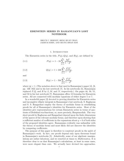
EISENSTEIN SERIES IN RAMANUJAN’S LOST<br />
NOTEBOOK<br />
BRUCE C. BERNDT, HENG HUAT CHAN,<br />
JAEBUM SOHN, AND SEUNG HWAN SON<br />
1. Introduction<br />
The <strong>Eisenste<strong>in</strong></strong> <strong>series</strong> <strong>in</strong> the title, P (q), Q(q), and R(q), are def<strong>in</strong>ed by<br />
∞�<br />
(1.1) P (q) := 1 − 24<br />
(1.2) Q(q) := 1 + 240<br />
and<br />
(1.3) R(q) := 1 − 504<br />
k=1<br />
∞�<br />
k=1<br />
∞�<br />
k=1<br />
kqk ,<br />
1 − qk k3qk ,<br />
1 − qk k5qk ,<br />
1 − qk where |q| < 1. (The notation above is that used <strong>in</strong> Ramanujan’s paper [4], [6,<br />
pp. 136–162] and <strong>in</strong> his <strong>lost</strong> <strong>notebook</strong> [7]. In his <strong>notebook</strong>s [5], Ramanujan<br />
replaced P, Q, and R by L, M, and N, respectively.) On pages 44, 50, 51,<br />
and 53 <strong>in</strong> his <strong>lost</strong> <strong>notebook</strong> [7], Ramanujan offers 12 formulas for <strong>Eisenste<strong>in</strong></strong><br />
<strong>series</strong>. All are connected with modular equations of either degree 5 or 7.<br />
In a wonderful paper [3] devoted to prov<strong>in</strong>g identities for <strong>Eisenste<strong>in</strong></strong> <strong>series</strong><br />
and <strong>in</strong>complete elliptic <strong>in</strong>tegrals <strong>in</strong> Ramanujan’s <strong>lost</strong> <strong>notebook</strong>, S. Raghavan<br />
and S. S. Rangachari employ the theory of modular forms <strong>in</strong> establish<strong>in</strong>g<br />
proofs for all of Ramanujan’s identities for <strong>Eisenste<strong>in</strong></strong> <strong>series</strong>. Most of the<br />
identities give representations for certa<strong>in</strong> <strong>Eisenste<strong>in</strong></strong> <strong>series</strong> <strong>in</strong> terms of quotients<br />
of Dedek<strong>in</strong>d eta-functions, or, more precisely, Hauptmoduls. The very<br />
short proofs by Raghavan and Rangachari depend upon the f<strong>in</strong>ite dimensions<br />
of the spaces of the relevant modular forms, and therefore upon show<strong>in</strong>g that<br />
a sufficient number of coefficients <strong>in</strong> the expansions about q = 0 of both sides<br />
of the proposed identities agree. Ramanujan evidently was unfamiliar with<br />
the theory of modular forms and most likely did not discover the identities<br />
by compar<strong>in</strong>g coefficients.<br />
The purpose of this paper is therefore to construct proofs <strong>in</strong> the spirit of<br />
Ramanujan’s work. In fact, our proofs depend only upon theorems found<br />
<strong>in</strong> Ramanujan’s <strong>notebook</strong>s [5]. Admittedly, some of our algebraic manipulations<br />
are rather laborious, and we resorted at times to Mathematica. It is<br />
therefore clear to us that Ramanujan’s calculations, at least <strong>in</strong> some cases,<br />
were more elegant than ours. We actually have devised two approaches.<br />
1
2 B. C. BERNDT, H. H. CHAN, J. SOHN, AND S. H. SON<br />
In Sections 3 and 4, we use the two methods, respectively, to prove Ramanujan’s<br />
qu<strong>in</strong>tic identities. At the end of Section 3, we prove a first order<br />
nonl<strong>in</strong>ear “qu<strong>in</strong>tic” differential equation of Ramanujan satisfied by P (q).<br />
In Section 5, we use the second approach, which is more constructive, to<br />
prove Ramanujan’s septic identities. The new parametrizations for moduli<br />
of degree 7 <strong>in</strong> Section 5 appear to more useful than those given <strong>in</strong> [1, Sect.<br />
19]. A subset of the authors plans to utilize these parametrizations <strong>in</strong> future<br />
work. Section 7 is devoted to prov<strong>in</strong>g two new first order nonl<strong>in</strong>ear “septic”<br />
differential equations for P (q).<br />
Page numbers placed after theorem numbers refer to their locations <strong>in</strong><br />
the <strong>lost</strong> <strong>notebook</strong> [7].<br />
As usual, set<br />
2. Prelim<strong>in</strong>ary Results<br />
(a; q)∞ :=<br />
Def<strong>in</strong>e, after Ramanujan,<br />
∞�<br />
(1 − aq n ), |q| < 1.<br />
n=0<br />
(2.1) f(−q) := (q; q)∞ =: e −2πiz/24 η(z), q = e 2πiz , Im z > 0,<br />
where η denotes the Dedek<strong>in</strong>d eta-function. We shall use the well-known<br />
transformation formula [1, p. 43, Entry 27(iii)]<br />
(2.2) η(−1/z) = � z/i η(z).<br />
If q = e 2πiz , Im z > 0, Q(q) and R(q) obey the well-known transformation<br />
formulas [8, p. 136]<br />
(2.3) Q(e −2πi/z ) = z 4 Q(e 2πiz )<br />
and<br />
(2.4) R(e −2πi/z ) = z 6 R(e 2πiz ).<br />
and<br />
Our proofs below depend upon modular equations. As usual, set<br />
2F1(a, b; c; x) :=<br />
(a)k :=<br />
∞�<br />
k=0<br />
Γ(a + k)<br />
Γ(a)<br />
Suppose that, for some positive <strong>in</strong>teger n,<br />
(2.5)<br />
2F1( 1<br />
2<br />
2F1( 1<br />
2<br />
1 , 2 ; 1; 1 − β)<br />
, 1<br />
2<br />
(a)k(b)k<br />
(c)kk! xk , |x| < 1.<br />
1<br />
2F1( 2 = n<br />
; 1; β)<br />
, 1<br />
2<br />
2F1( 1<br />
2<br />
; 1; 1 − α)<br />
.<br />
; 1; α)<br />
A modular equation of degree n is an equation <strong>in</strong>volv<strong>in</strong>g α and β that is<br />
<strong>in</strong>duced by (2.5). We often say that β has degree n over α. Also set<br />
(2.6) z1 := 2F1( 1 1<br />
2 ,<br />
, 1<br />
2<br />
2 ; 1; α) and zn := 2F1( 1<br />
2<br />
1 , 2 ; 1; β).
The multiplier m is def<strong>in</strong>ed by<br />
(2.7) m := z1<br />
.<br />
When<br />
and z = 2F1( 1<br />
2<br />
(2.8)<br />
(2.9)<br />
and<br />
q = exp<br />
EISENSTEIN SERIES 3<br />
�<br />
−π<br />
zn<br />
2F1( 1<br />
2<br />
, 1<br />
2<br />
2F1( 1<br />
2<br />
�<br />
; 1; 1 − x)<br />
, 1<br />
2<br />
; 1; x)<br />
1 , 2 ; 1; x), we have the “evaluations”<br />
f(−q 2 ) = √ z 2 −1/3 (x(1 − x)/q) 1/12 ,<br />
Q(q 2 ) = z 4 (1 − x + x 2 ),<br />
(2.10) R(q 2 ) = z 6 (1 + x)(1 − x/2)(1 − 2x).<br />
These are, respectively, Entries 12(iii), 13(i), and 13(ii) <strong>in</strong> Chapter 17 of<br />
Ramanujan’s second <strong>notebook</strong> [1, pp. 124, 126].<br />
Next, we record some relations from the theory of modular equations of<br />
degree 5. Set<br />
(2.11) m = 1 + 2p, 0 < p < 2,<br />
and<br />
(2.12) ρ = (m 3 − 2m 2 + 5m) 1/2 .<br />
Then [1, p. 284, eqs. (13.4), (13.5)]<br />
� �<br />
α5 1/8<br />
(2.13)<br />
=<br />
β<br />
5ρ + m2 + 5m<br />
4m2 ,<br />
(2.14)<br />
� �<br />
(1 − α) 5 1/8<br />
1 − β<br />
= 5ρ − m2 − 5m<br />
4m 2 , and<br />
Furthermore [1, p. 288, Entry 14(ii)]<br />
(2.15) 4α(1 − α) = p<br />
and<br />
(2.16) 4β(1 − β) = p 5<br />
� �<br />
β5 1/8<br />
=<br />
α<br />
ρ − m − 1<br />
� �<br />
(1 − β) 5 1/8<br />
=<br />
1 − α<br />
ρ + m + 1<br />
� �5 2 − p<br />
1 + 2p<br />
� �<br />
2 − p<br />
.<br />
1 + 2p<br />
,<br />
4<br />
.<br />
4<br />
Also, from Entry 14(iii) <strong>in</strong> Chapter 19 of Ramanujan’s second <strong>notebook</strong> [1,<br />
p. 289]<br />
(2.17) 1 − 2β = (1 + p − p 2 � �<br />
1 + p2 1/2<br />
)<br />
.<br />
1 + 2p
4 B. C. BERNDT, H. H. CHAN, J. SOHN, AND S. H. SON<br />
We also need two modular equations of degree 5 from Entry 13(iv) of<br />
Chapter 18 <strong>in</strong> Ramanujan’s second <strong>notebook</strong> [1, p. 281], namely,<br />
(2.18) m = 1 + 2 4/3<br />
� �<br />
β5 (1 − β) 5 1/24<br />
α(1 − α)<br />
and<br />
(2.19)<br />
5<br />
= 1 + 24/3<br />
m<br />
� α 5 (1 − α) 5<br />
β(1 − β)<br />
� 1/24<br />
.<br />
For Section 4, we need several modular equations of degree 7 found <strong>in</strong><br />
Entry 19(i), (ii), (iii), and (vii) of Ramanujan’s second <strong>notebook</strong> [1, pp.<br />
314-315]. Thus, if β has degree 7 over α and m is the multiplier of degree 7,<br />
(2.20) (αβ) 1/8 + {(1 − α)(1 − β)} 1/8 = 1,<br />
(2.21)<br />
(2.22)<br />
(2.23)<br />
(2.24)<br />
and<br />
(2.25)<br />
m = −<br />
7<br />
m =<br />
1 − 4<br />
� β 7 (1 − β) 7<br />
α(1 − α)<br />
� 1/24<br />
(αβ) 1/8 ,<br />
1/8<br />
− {(1 − α)(1 − β)}<br />
� �<br />
α7 (1 − α) 7 1/24<br />
1 − 4<br />
β(1 − β)<br />
(αβ) 1/8 ,<br />
1/8<br />
− {(1 − α)(1 − β)}<br />
� �<br />
(1 − β) 7 1/8 � �<br />
β7 1/8<br />
−<br />
1 − α α<br />
��<br />
= m<br />
� �<br />
α7 1/8 � �<br />
(1 − α) 7 1/8<br />
−<br />
β<br />
1 − β<br />
= 7<br />
m<br />
m − 7<br />
m<br />
1 + (αβ) 1/2 + {(1 − α)(1 − β)} 1/2�<br />
��<br />
1 + (αβ) 1/2 + {(1 − α)(1 − β)} 1/2�<br />
/2<br />
�<br />
= 2<br />
×<br />
(αβ) 1/8 − {(1 − α)(1 − β)} 1/8�<br />
�1/2 /2 ,<br />
�1/2 ,<br />
�<br />
2 + (αβ) 1/4 + {(1 − α)(1 − β)} 1/4�<br />
.<br />
3. Qu<strong>in</strong>tic Identities (First Method)<br />
Theorem 3.1 (p. 50). For Q(q) and f(−q) def<strong>in</strong>ed by (1.2) and (2.1),<br />
respectively,<br />
(3.1) Q(q) = f 10 (−q)<br />
f 2 (−q5 ) + 250qf 4 (−q)f 4 (−q 5 ) + 3125q 2 f 10 (−q5 )<br />
f 2 (−q)<br />
and<br />
(3.2) Q(q 5 ) = f 10 (−q)<br />
f 2 (−q 5 ) + 10qf 4 (−q)f 4 (−q 5 ) + 5q 2 f 10 (−q 5 )<br />
f 2 (−q) .
EISENSTEIN SERIES 5<br />
Proof. It is slightly advantageous to first prove (3.2) with q replaced by q 2 .<br />
To prove (3.2), we first write the right side of (3.2) as a function of p, where<br />
p is def<strong>in</strong>ed by (2.11).<br />
By (2.8),<br />
(3.3)<br />
q 4 f 10 (−q10 )<br />
f 2 (−q2 ) = q4 z5 52−10/3 � β(1 − β)/q5�5/6 z12−2/3 (α(1 − α)/q) 1/6<br />
= 2 −8/3 z4 5<br />
m<br />
� β 5 (1 − β) 5<br />
α(1 − α)<br />
� 1/6<br />
,<br />
where β has degree 5 over α, z1 and z5 are def<strong>in</strong>ed by (2.6), and m is the<br />
multiplier def<strong>in</strong>ed by (2.7). Us<strong>in</strong>g (2.13), (2.14), (2.12), and (2.11) <strong>in</strong> (3.3),<br />
we f<strong>in</strong>d that<br />
(3.4)<br />
q 4 f 10 (−q 10 )<br />
f 2 (−q 2 ) = 2−8/3 z4 5<br />
m<br />
= z4 5 (m − 1)4<br />
28m � ρ 2 − (m + 1) 2<br />
=<br />
16<br />
z 4 5 p4<br />
2 4 (1 + 2p) .<br />
� 4/3<br />
Similarly, from (2.8), (2.7), (2.15), (2.16), and (2.11),<br />
f 6 (−q2 )<br />
q2f 6 (−q10 )<br />
=<br />
=<br />
� �1/2 α(1 − α)<br />
m3<br />
β(1 − β)<br />
m 3<br />
� �2 2 − p<br />
=<br />
p(1 + 2p)<br />
(1 + 2p)(2 − p)2<br />
p2 (3.5)<br />
.<br />
Thus, from (3.4) and (3.5),<br />
=<br />
=<br />
= z 4 5<br />
q 4 f 10 (−q10 )<br />
f 2 (−q2 �<br />
f 12 (−q2 )<br />
) q4f 12 (−q10 ) + 10 f 6 (−q2 )<br />
q2f 6 (−q10 )<br />
z4 5p4 24 �<br />
(1 + 2p) 2 (2 − p) 4<br />
(1 + 2p) p4 z4 5<br />
24 (1 + 2p) (16 + 32p − 8p5 + 4p 6 )<br />
�<br />
1 + p5 �<br />
(−2 + p)<br />
4(1 + 2p)<br />
= z 4 5(1 − β(1 − β))<br />
= Q(q 10 ),<br />
�<br />
+ 5<br />
(1 + 2p)(2 − p)2<br />
+ 10<br />
p2 + 5<br />
where <strong>in</strong> the penultimate step we used (2.16), and <strong>in</strong> the last step utilized<br />
(2.9). This completes the proof of (3.2).<br />
To prove (3.1), we first rewrite (3.2) <strong>in</strong> terms of the Dedek<strong>in</strong>d eta-function,<br />
def<strong>in</strong>ed <strong>in</strong> (2.1). Accord<strong>in</strong>gly,<br />
(3.6) Q(q 5 ) = η10 (5z)<br />
η 2 (z)<br />
�� �12 η(z)<br />
η(5z)<br />
� � �<br />
6<br />
η(z)<br />
+ 10 + 5 .<br />
η(5z)<br />
�
6 B. C. BERNDT, H. H. CHAN, J. SOHN, AND S. H. SON<br />
We now transform (3.6) by means of (2.2) and (2.3) to deduce that<br />
or<br />
(5z/i) 5<br />
(z/i)<br />
η2 (−1/z)<br />
� �12 � � � ⎞<br />
6<br />
5z/i<br />
η(−1/z) 5z/i<br />
+ 10 � + 5⎠<br />
,<br />
η(−1/(5z))<br />
z/i η(−1/(5z))<br />
(5z) −4 Q(e −2πi/(5z) ) = η10 (−1/(5z))<br />
⎛�<br />
× ⎝<br />
η(−1/z)<br />
�<br />
z/i<br />
Q(e −2πi/(5z) )<br />
= η10 (−1/(5z))<br />
η2 �<br />
5<br />
(−1/z)<br />
5<br />
� �12 � � �<br />
6<br />
η(−1/z)<br />
η(−1/z)<br />
+ 250<br />
+ 1<br />
η(−1/(5z))<br />
η(−1/(5z))<br />
= 5 5 η10 (−1/z)<br />
η2 (−1/(5z)) + 250η4 (−1/(5z))η 4 (−1/z) + η10 (−1/(5z))<br />
η2 (−1/z)<br />
If we set q = e −2πi/(5z) and use (2.1), the last equality takes the shape (3.1),<br />
and so this completes the proof of (3.1). �<br />
Theorem 3.2 (p. 51). For f(−q) and R(q) def<strong>in</strong>ed by (2.1) and (1.3),<br />
respectively,<br />
R(q) =<br />
(3.7)<br />
and<br />
(3.8)<br />
� f 15 (−q)<br />
×<br />
R(q 5 ) =<br />
f 3 (−q 5 ) − 500qf 9 (−q)f 3 (−q 5 ) − 15625q 2 f 3 (−q)f 9 (−q 5 )<br />
�<br />
1 + 22q f 6 (−q5 )<br />
f 6 (−q) + 125q2 f 12 (−q5 )<br />
f 12 (−q)<br />
� f 15 (−q)<br />
×<br />
f 3 (−q 5 ) + 4qf 9 (−q)f 3 (−q 5 ) − q 2 f 3 (−q)f 9 (−q 5 )<br />
�<br />
1 + 22q f 6 (−q 5 )<br />
f 6 (−q) + 125q2 f 12 (−q 5 )<br />
f 12 (−q) .<br />
Proof. Our procedure is similar to that of the previous theorem. We establish<br />
(3.8) first, but with q replaced by q 2 .<br />
By (2.8), (2.7), (2.15), and (2.16),<br />
(3.9)<br />
f 15 (−q 2 )<br />
f 3 (−q 10 )<br />
z15/2 1 =<br />
16z 3/2<br />
5<br />
� α 5 (1 − α) 5<br />
β(1 − β)<br />
� 1/4<br />
= z6 1 m3/2<br />
64<br />
.<br />
�<br />
� �6 2 − p<br />
.<br />
1 + 2p<br />
�
Hence, from (3.9), (3.5), (2.7), and (2.11),<br />
(3.10)<br />
F (q) := f 15 (−q2 )<br />
f 3 (−q10 )<br />
×<br />
�<br />
= z6 1 m3/2<br />
=<br />
=<br />
EISENSTEIN SERIES 7<br />
�<br />
1 + 4q 2 f 6 (−q10 )<br />
f 6 (−q2 ) − q4 f 12 (−q10 )<br />
f 12 (−q2 )<br />
1 + 22q2 f 6 (−q10 )<br />
f 6 (−q2 ) + 125q4 f 12 (−q10 )<br />
f 12 (−q2 )<br />
� �6 2 − p<br />
64 1 + 2p<br />
�<br />
p<br />
× 1 + 4<br />
2<br />
−<br />
(1 + 2p)(2 − p) 2<br />
�<br />
p<br />
× 1 + 22<br />
2<br />
+ 125<br />
(1 + 2p)(2 − p) 2<br />
�<br />
p4 (1 + 2p) 2 (2 − p) 4<br />
�<br />
p 4<br />
(1 + 2p) 2 (2 − p) 4<br />
z6 5<br />
8m3/2 � 2 3 4 5 6<br />
4 + 8p − 6p − 6p + 9p − 5p + p �<br />
× � 4 + 8p + 12p2 + 12p3 + 9p4 + 4p5 + p6 z6 5<br />
8m3/2 (1 + p − p2 )(4 + 4p − 6p 2 + 4p 3 − p 4 )<br />
× � (1 + p2 )(4 + 8p + 8p2 + 4p3 + p4 ).<br />
Us<strong>in</strong>g (2.17) and (2.11), we can write (3.10) <strong>in</strong> the form<br />
F (q) = z 6 5(1 − 2β) 4 + 4p − 6p2 + 4p3 − p4 �<br />
4 + 8p + 8p2 + 4p3 + p4 8(1 + 2p)<br />
(3.11)<br />
= z 6 5(1 − 2β) (4 + 4p − 6p2 + 4p3 − p4 )(2 + 2p + p2 )<br />
8(1 + 2p)<br />
= z 6 5(1 − 2β) 8 + 16p + 2p5 − p6 8(1 + 2p)<br />
= z 6 �<br />
5(1 − 2β) 1 + p5 �<br />
(2 − p)<br />
8(1 + 2p)<br />
= z 6 5(1 − 2β) � 1 + 1<br />
2β(1 − β)�<br />
= z 6 5(1 − 2β)(1 − 1<br />
2β)(1 + β)<br />
= R(q 10 ),<br />
where <strong>in</strong> the antipenultimate l<strong>in</strong>e we used (2.16), and <strong>in</strong> the last l<strong>in</strong>e we used<br />
(2.10). Comb<strong>in</strong><strong>in</strong>g (3.10) and (3.11), we deduce (3.8), but with q replaced<br />
by q 2 .<br />
The proof of (3.7) is almost exactly like the proof of (3.1), but, of course,<br />
we use (2.4) <strong>in</strong>stead of (2.3). �<br />
The next two results are algebraic comb<strong>in</strong>ations of the pairs of representations<br />
<strong>in</strong> Theorems 3.1 and 3.2.
8 B. C. BERNDT, H. H. CHAN, J. SOHN, AND S. H. SON<br />
Theorem 3.3 (p. 51). Let A = Q(q) and B = Q(q 5 ). Then<br />
� A 2 + 94AB + 625B 2<br />
(3.12)<br />
Proof. Set<br />
= 12 √ �<br />
f 10 (−q)<br />
5<br />
f 2 (−q5 ) + 26qf 4 (−q)f 4 (−q 5 ) + 125q 2 f 10 (−q5 )<br />
f 2 �<br />
.<br />
(−q)<br />
(3.13) C = f 5 (−q)<br />
f(−q 5 ) , D = qf 4 (−q)f 4 (−q 5 ), and E = q f 5 (−q 5 )<br />
f(−q) .<br />
Note that<br />
(3.14) CE = D.<br />
Equalities (3.1) and (3.2) now take the shapes<br />
(3.15) A = C 2 + 250D + 3125E 2<br />
and B = C 2 + 10D + 5E 2 ,<br />
respectively, and the proposed equality (3.12) has the form<br />
(3.16)<br />
� A 2 + 94AB + 625B 2 = 12 √ 5 � C 2 + 26D + 125E 2 � .<br />
Substitute (3.15) <strong>in</strong>to (3.16), square both sides, use (3.14), and with just<br />
elementary algebra (3.16) is then verified. �<br />
Theorem 3.4 (p. 51). Let A = R(q) and B = R(q 5 ). Then<br />
� 5(A + 125B) 2 − (126) 2 AB<br />
(3.17)<br />
�<br />
f 10 (−q)<br />
= 252<br />
×<br />
�<br />
f 2 (−q5 ) + 62qf 4 (−q)f 4 (−q 5 ) + 125q 2 f 10 (−q5 )<br />
f 2 (−q)<br />
f 10 (−q)<br />
f 2 (−q5 ) + 22qf 4 (−q)f 4 (−q5 ) + 125q2 f 10 (−q5 )<br />
f 2 (−q) .<br />
Proof. We employ the notation (3.13). Equalities (3.7) and (3.8) then may<br />
be written as, respectively,<br />
(3.18) A = � C 3 − 500CD − 5 6 DE � � 1 + 22E 2 /D + 125E 4 /D 2<br />
and<br />
(3.19) B = � C 3 + 4CD − DE � � 1 + 22E 2 /D + 125E 4 /D 2 ,<br />
and the proposed equality (3.17) has the form<br />
� 5(A + 125B) 2 − (126) 2 AB = 252(C 2 + 62D + 125E 2 )<br />
(3.20)<br />
× � C 2 + 22D + 125E 2 .<br />
Square (3.20), use (3.18), (3.19), and (3.14), and simplify to verify the truth<br />
of (3.20). �<br />
Our next goal is to establish a differential equation satisfied by P (q),<br />
def<strong>in</strong>ed by (1.1). We need two lemmas.<br />
�
EISENSTEIN SERIES 9<br />
Lemma 3.5. Recall that Q(q) and R(q) are def<strong>in</strong>ed by (1.2) and (1.3),<br />
respectively. Let<br />
(3.21) u := q 1/4 f(−q)f(−q 5 ) and λ := q<br />
Then<br />
(3.22) Q(q) = u 4<br />
and<br />
(3.23) R(q) = u 6<br />
�<br />
1<br />
λ + 250 + 55 �<br />
λ<br />
�<br />
1<br />
λ − 500 − 56 � �<br />
1<br />
λ + 22 + 125λ.<br />
λ<br />
� �<br />
f(−q5 6<br />
)<br />
.<br />
f(−q)<br />
Proof. Identities (3.22) and (3.23) are obta<strong>in</strong>ed from (3.1) and (3.7), respectively.<br />
For example, by (3.1) and (3.21),<br />
� �<br />
f 6 (−q)<br />
Q(q) = qf 4 (−q)f 4 (−q 5 )<br />
= u 4<br />
�<br />
1<br />
λ + 250 + 55 �<br />
λ .<br />
qf 6 (−q5 ) + 250 + 3125q f 6 (−q5 )<br />
f 6 (−q)<br />
Lemma 3.6. Recall that f(−q) is def<strong>in</strong>ed by (2.1). Then<br />
1 +<br />
∞� kq<br />
6<br />
k=1<br />
k ∞� kq<br />
− 30<br />
1 − qk k=1<br />
5k<br />
1 − q5k �<br />
=<br />
f 12 (−q) + 22qf 6 (−q)f 6 (−q5 ) + 125q2f 12 (−q5 )<br />
f 2 (−q)f 2 (−q5 .<br />
)<br />
Lemma 3.6 is part of Entry 4(i) <strong>in</strong> Chapter 21 of Ramanujan’s second<br />
<strong>notebook</strong>, and a proof is given <strong>in</strong> [1, p. 463]. We give here a new short<br />
proof, based on Lemma 3.5.<br />
Proof. Us<strong>in</strong>g Ramanujan’s differential equations [4, eq. 30], [6, p. 142],<br />
(3.24) q dQ<br />
dq<br />
we deduce that<br />
= P Q − R<br />
3<br />
and q dR<br />
dq<br />
(3.25) Q 3 − R 2 = 3qR dQ<br />
dq<br />
From (3.22) and (3.23), we f<strong>in</strong>d that<br />
(3.26) Q 3 − R 2 = 1728 u12<br />
(3.27)<br />
dQ<br />
dq<br />
= 4u3<br />
− 2qQdR<br />
dq .<br />
,<br />
λ2 �<br />
1<br />
λ + 250 + 55 �<br />
du<br />
λ + u4<br />
dq<br />
P R − Q2<br />
= ,<br />
2<br />
�<br />
− 1<br />
+ 55<br />
λ2 �<br />
dλ<br />
dq ,<br />
�
10 B. C. BERNDT, H. H. CHAN, J. SOHN, AND S. H. SON<br />
and<br />
(3.28)<br />
dR<br />
dq<br />
= 6u5<br />
�<br />
1<br />
λ − 500 − 56 � �<br />
1<br />
λ + 22 + 125λdu<br />
λ dq<br />
− 3u6 (1 − 152λ + 5250λ2 + 250000λ3 + 1953125λ4 )<br />
2λ3 dλ<br />
�<br />
1<br />
dq<br />
+ 22 + 125λ<br />
λ<br />
Us<strong>in</strong>g (3.22), (3.23), (3.27), and (3.28) to simplify the right hand side of<br />
(3.25), we deduce that<br />
Q 3 − R 2 = 3qR dQ<br />
u<br />
− 2qQdR = 1728<br />
dq dq 10<br />
λ3 � q<br />
1<br />
+ 22 + 125λ<br />
λ dλ<br />
dq .<br />
Comb<strong>in</strong><strong>in</strong>g this last equation with (3.26) yields<br />
(3.29) q dλ<br />
dq = u2 �<br />
1<br />
λ + 22 + 125λ.<br />
λ<br />
On the other hand, by straightforward logarithmic differentiation,<br />
(3.30) q dλ<br />
�<br />
∞� kq<br />
= λ 1 − 30<br />
dq 5k ∞� kq<br />
+ 6<br />
1 − q5k k<br />
1 − qk �<br />
.<br />
k=1<br />
If we comb<strong>in</strong>e (3.29) and (3.30), we deduce Lemma 3.6. �<br />
k=1<br />
Theorem 3.7 (p. 44). Let P (q) be def<strong>in</strong>ed by (1.1). Then<br />
�� �<br />
1 + 22λ + 125λ2 − 30F (λ)<br />
(3.31) P (q) = f 5 (−q)<br />
f(−q 5 )<br />
and<br />
(3.32) P (q 5 ) = f 5 (−q)<br />
f(−q 5 )<br />
�� �<br />
1 + 22λ + 125λ2 − 6F (λ) ,<br />
where λ is def<strong>in</strong>ed <strong>in</strong> (3.21), and where F (λ) satisfies the nonl<strong>in</strong>ear, first<br />
order differential equation<br />
(3.33) 1 + 25 5<br />
λ +<br />
2 2λ F 2 (λ) = F ′ (λ) � 1 + 22λ + 125λ2 .<br />
Proof. Assume that F (λ) is def<strong>in</strong>ed by (3.31), so that (3.31) is trivially true.<br />
By (1.1) and Lemma 3.6, we have<br />
5P (q<br />
(3.34)<br />
5 ) − P (q)<br />
=<br />
4<br />
f 5 (−q)<br />
f(−q5 �<br />
1 + 22λ + 125λ2 ,<br />
)<br />
with λ def<strong>in</strong>ed by (3.21). If we substitute (3.31) <strong>in</strong>to (3.34) and solve for<br />
P (q5 ), we deduce (3.32). It rema<strong>in</strong>s to prove that F (λ) satisfies the differential<br />
equation (3.33).<br />
From (3.24), (3.22), (3.23), and (3.29), we f<strong>in</strong>d that, with the prime ′<br />
denot<strong>in</strong>g differentiation with respect to q,<br />
(3.35) P (q) = 12q u′<br />
u<br />
− 2 u2<br />
√ λ<br />
� 1 + 22λ + 125λ 2 .
EISENSTEIN SERIES 11<br />
Differentiat<strong>in</strong>g (3.35) with the help of (3.29), we deduce that<br />
(3.36)<br />
q dP<br />
dq = −u4 125λ2 − 1<br />
− 4<br />
λ<br />
u2<br />
�<br />
√ q<br />
λ<br />
u′<br />
�<br />
�1<br />
�<br />
+ 22λ + 125λ2 + 12q q<br />
u<br />
u′<br />
� ′<br />
.<br />
u<br />
Next, by us<strong>in</strong>g another differential equation of Ramanujan [4, eq. (30)], [6,<br />
p. 142],<br />
(3.37) q dP<br />
dq = P 2 − Q<br />
,<br />
12<br />
(3.22), (3.23), (3.35), and (3.36), we conclude that<br />
�<br />
(3.38) 12q q u′<br />
� ′ �<br />
− 12 q<br />
u<br />
u′<br />
�2 u<br />
= − 3 u<br />
4<br />
4 � � 2<br />
1 + 125λ + 18λ .<br />
λ<br />
We now identify Ramanujan’s function F (λ). By compar<strong>in</strong>g (3.31) and<br />
(3.35), we conclude that<br />
(3.39) F (λ) = − 2<br />
√<br />
u′ λ 1 �<br />
q + 1 + 22λ + 125λ2 .<br />
5 u u2 10<br />
Rewrit<strong>in</strong>g (3.39) <strong>in</strong> the form,<br />
(3.40)<br />
F (λ)<br />
√ λ − 1<br />
10 √ λ<br />
� 2 u′<br />
1 + 22λ + 125λ2 = − q<br />
5 u<br />
1<br />
,<br />
u2 and differentiat<strong>in</strong>g with respect to q, we deduce that<br />
− 1 u<br />
2<br />
2<br />
�<br />
1 + 22λ + 125λ2 √ F (λ) +<br />
λ λ<br />
1 dF (λ) u2 125λ<br />
√ q −<br />
λ dq 20<br />
2 − 1<br />
λ<br />
(3.41) = − 2<br />
� �<br />
q q<br />
5<br />
u′<br />
� ′<br />
1 2<br />
−<br />
u u2 u2 �<br />
q u′<br />
� �<br />
2<br />
.<br />
u<br />
Us<strong>in</strong>g (3.38) and (3.40), we may rewrite the right hand side of (3.41) and<br />
deduce that<br />
− 1 u<br />
2<br />
2<br />
�<br />
1 + 22λ + 125λ2 √ F (λ) +<br />
λ λ<br />
1 dF (λ) u2 125λ<br />
√ q −<br />
λ dq 20<br />
2 − 1<br />
λ<br />
2 1 + 18λ + 125λ2<br />
= u +<br />
40λ<br />
5<br />
2 u2 F 2 (λ) 1 + 22λ + 125λ2<br />
+ u2<br />
λ 40λ<br />
(3.42)<br />
2 1<br />
−u<br />
2λ F (λ)�1 + 22λ + 125λ2 .<br />
Simplify<strong>in</strong>g (3.42) with the use of (3.29), we deduce Ramanujan’s differential<br />
equation (3.33). �
12 B. C. BERNDT, H. H. CHAN, J. SOHN, AND S. H. SON<br />
4. Qu<strong>in</strong>tic Identities (Second Method)<br />
The alternative method to prov<strong>in</strong>g Theorems 3.1, 3.2, and 3.7 that we<br />
present <strong>in</strong> this section is more constructive than that <strong>in</strong> Section 3, but, although<br />
no less elementary, is perhaps slightly more removed from procedures<br />
that Ramanujan might have employed. On the other hand, the method here<br />
is more amenable to prov<strong>in</strong>g further theorems of this sort, especially if one<br />
does not know their formulations beforehand.<br />
We beg<strong>in</strong> by <strong>in</strong>troduc<strong>in</strong>g some simplify<strong>in</strong>g notation and mak<strong>in</strong>g some<br />
useful prelim<strong>in</strong>ary calculations. Set<br />
(4.1)<br />
(4.2)<br />
and<br />
p1 :=<br />
p2 :=<br />
(4.3) C :=<br />
� β 5 (1 − β) 5<br />
α(1 − α)<br />
� α 5 (1 − α) 5<br />
β(1 − β)<br />
� z 5 5<br />
16 √ .<br />
z1<br />
Observe that, by (2.18) and (2.19), respectively,<br />
(4.4) p1 =<br />
and<br />
(4.5) p2 =<br />
It follows that<br />
(4.6) α(1 − α) = p1p 5 2 =<br />
and<br />
(4.7) β(1 − β) = p 5 1p2 =<br />
(4.8)<br />
and<br />
(4.9)<br />
We also note that, by (4.3),<br />
S<strong>in</strong>ce, by (4.3),<br />
C 3 =<br />
z4 1<br />
162 =<br />
m5 z 4 5<br />
16 2 m =<br />
� z 15<br />
5<br />
16 3� z 3 1<br />
m − 1<br />
2 4/3<br />
m − 1<br />
2 4/3<br />
5 − m<br />
2 4/3 m .<br />
� 1/24<br />
,<br />
� 1/24<br />
,<br />
�<br />
5 − m<br />
24/3 �5 (m − 1)(m − 5)5<br />
= −<br />
m<br />
162m5 � �5 m − 1 5 − m<br />
2 4/3<br />
z 4 1<br />
16 2 (z1/z5) 5 = z5 5<br />
16 2 z1<br />
z 4 5<br />
16 2 (z1/z5) = z5 5<br />
16 2 z1<br />
= z6 5<br />
16 3<br />
24/3m = −(m − 1)5 (m − 5)<br />
162 .<br />
m<br />
1<br />
� =<br />
(z1/z3) 3<br />
= C 2<br />
= C 2 .<br />
z 6 5<br />
16 3 m √ m ,
we f<strong>in</strong>d that<br />
(4.10)<br />
z6 1<br />
163 =<br />
m6 EISENSTEIN SERIES 13<br />
z 6 1<br />
16 3 (z 6 1 /z6 5 ) = z6 5<br />
16 3 = C3 m √ m.<br />
We shall use (4.8)–(4.10) <strong>in</strong> our alternative proofs of Theorems 3.1 and 3.2.<br />
In view of (3.1), it is natural to <strong>in</strong>troduce abbreviated notation for certa<strong>in</strong><br />
quotients of eta-functions. Our goal is to represent these quotients as<br />
polynomials <strong>in</strong> the multiplier m. First, by (2.8), (4.3), (4.2), and (4.5),<br />
(4.11)<br />
r1 : = f 5 (−q 2 )<br />
=<br />
= 16C<br />
f(−q 10 ) =<br />
� z 5 5 z 3 1<br />
2 4/3√ z1z 3 5<br />
2 4/3 m3 p 2 2 = 16C<br />
= Cm(m − 5) 2 ,<br />
and, by (2.8), (4.3), (4.1), and (4.4),<br />
(4.12)<br />
r2 : = q 2 f 5 (−q 10 )<br />
=<br />
f(−q 2 )<br />
� z 5 5<br />
2 4/3√ z1<br />
� z 5 1 2 −5/3 (α(1 − α)/q) 5/12<br />
√ z52 −1/3 (β(1 − β)/q 5 ) 1/12<br />
� α 5 (1 − α) 5<br />
= q2<br />
= 16C<br />
24/3 p21 = 16C<br />
24/3 = C(m − 1) 2 .<br />
Hence, by (4.11) and (4.12),<br />
� β 5 (1 − β) 5<br />
� 1/12<br />
β(1 − β)<br />
�<br />
5 − m<br />
m3<br />
24/3 24/3 �2 m<br />
� z 5 5 2 −5/3 (β(1 − β)/q 5 ) 5/12<br />
√ z12 −1/3 (α(1 − α)/q) 1/12<br />
� 1/12<br />
α(1 − α)<br />
� �2 m − 1<br />
2 4/3<br />
(4.13) r1r2 = q 2 f 4 (−q 2 )f 4 (−q 10 ) = C 2 m(m − 5) 2 (m − 1) 2 .<br />
The follow<strong>in</strong>g lemma will be very useful.<br />
Lemma 4.1. Let<br />
g(m) := C 2<br />
�<br />
6�<br />
ckm k<br />
�<br />
.<br />
k=0<br />
If furthermore, we set, for some numbers x1, x2, and x3,<br />
then<br />
g(m) = x1r 2 1 + x2r1r2 + x3r 2 2,<br />
x1 = c6, x2 = c5 + 20c6, and x3 = c0.
14 B. C. BERNDT, H. H. CHAN, J. SOHN, AND S. H. SON<br />
Proof. S<strong>in</strong>ce, by (4.11)–(4.13),<br />
x1r 2 1 + x2r1r2 + x3r 2 2<br />
= C 2� x3 + m(25x2 − 4x3) + m 2 (625x1 − 60x2 + 6x3)<br />
+m 3 (−500x1 + 46x2 − 4x3) + m 4 (150x1 − 12x2 + x3)<br />
+m 5 (−20x1 + x2) + m 6 x1<br />
by match<strong>in</strong>g the coefficients of m k , k = 0, . . . , 6, we f<strong>in</strong>d that<br />
c0 = x3,<br />
c1 = 25x2 − 4x3,<br />
� ,<br />
c2 = 625x1 − 60x2 + 6x3,<br />
c3 = −500x1 + 46x2 − 4x3,<br />
c4 = 150x1 − 12x2 + x3,<br />
c5 = −20x1 + x2,<br />
c6 = x1.<br />
Therefore, if the system above is not overdeterm<strong>in</strong>ed, then g(m) can be<br />
expressed as a l<strong>in</strong>ear comb<strong>in</strong>ation of r2 1 , r1r2, and r2 2 . By solv<strong>in</strong>g the l<strong>in</strong>ear<br />
system of equations,<br />
c0 = x3,<br />
c5 = −20x1 + x2,<br />
c6 = x1,<br />
for x1, x2, and x3, and not<strong>in</strong>g that c1, c2, c3, and c4 are then uniquely determ<strong>in</strong>ed,<br />
we complete the proof. �<br />
We are now ready for our second proof of Theorem 3.1.<br />
Proof of Theorem 3.1. By (2.9), (4.6), and (4.8),<br />
Q(q 2 ) = z 4� �<br />
1 1 − α(1 − α)<br />
�<br />
1 +<br />
�<br />
(m − 1)(m − 5)5<br />
= z 4 1<br />
162m5 =<br />
z4 1<br />
162m5 � 2 5 5<br />
16 m + (m − 1)(m − 5) �<br />
= C 2 (m 6 + 230m 5 + · · · + 5 5 )<br />
= r 2 1 + 2 · 5 3 r1r2 + 5 5 r 2 2,<br />
upon the use of Lemma 4.1. Replac<strong>in</strong>g q 2 by q, we complete the proof of<br />
(3.1).
By (2.9), (4.7), and (4.9),<br />
EISENSTEIN SERIES 15<br />
Q(q 10 ) = z 4� �<br />
5 1 − β(1 − β)<br />
= z 4 5<br />
=<br />
�<br />
1 + (m − 1)5 (m − 5)<br />
z 4 5<br />
16 2 m<br />
16 2 m<br />
�<br />
� 16 2 m + (m − 1) 5 (m − 5) �<br />
= C 2 (m 6 − 10m 5 + · · · + 5)<br />
= r 2 1 + 10r1r2 + 5r 2 2,<br />
by an application of Lemma 4.1. Replac<strong>in</strong>g q 2 by q, we complete the proof<br />
of (3.2). �<br />
and<br />
For the proof of Theorem 3.2, it will be convenient to def<strong>in</strong>e<br />
D := m 2 − 2m + 5,<br />
E := m 2 + 2m + 5,<br />
F := m 2 + 20m − 25,<br />
G := m 2 − 4m − 1.<br />
Solv<strong>in</strong>g (4.6) and (4.7) and us<strong>in</strong>g the notation above, we deduce that<br />
(4.14) α = 1<br />
2 +<br />
�<br />
D/mF<br />
16m2 and<br />
(4.15) β = 1<br />
2 +<br />
�<br />
D/mG<br />
.<br />
16<br />
(See also [1, p. 289, eq. (14.2); p. 290, eq. (14.4)].)<br />
Us<strong>in</strong>g the notation above and Lemma 4.1, we may readily deduce the<br />
follow<strong>in</strong>g lemma<br />
Lemma 4.2. For D, E, F, and G def<strong>in</strong>ed above, for C def<strong>in</strong>ed by (4.3), and<br />
for r1 and r2, def<strong>in</strong>ed <strong>in</strong> (4.11) and (4.12), respectively, we have<br />
and<br />
C 2 DE 2 = r 2 1 + 22r1r2 + 5 3 r 2 2,<br />
C 2 F (m 4 − 540m 3 + 1350m 2 − 14 · 5 3 m + 5 4 ) = r 2 1 − 4 · 5 3 r1r2 − 5 6 r 2 2,<br />
C 2 G(m 4 − 12m 3 + 54m 2 − 108m + 1) = r 2 1 + 4r1r2 − r 2 2.
16 B. C. BERNDT, H. H. CHAN, J. SOHN, AND S. H. SON<br />
Proof of Theorem 3.2. By (2.10), (4.14), (4.10), and Lemma 4.2,<br />
R(q 2 ) = z 6 1(1 + α)(1 − α/2)(1 − 2α)<br />
�<br />
D/mF<br />
= z 6 1<br />
163m6 ( � D/mF − 24m 2 )( � D/mF + 24m 2 )<br />
z<br />
=<br />
6 1<br />
163m6 � � 2 2 4<br />
D/mF (D/m)F − 24 m �<br />
= (C 3 m √ m) � D/mF � E � m 4 − 540m 3 + 1350m 2<br />
−14 · 5 3 m + 5 4� /m �<br />
= √ C2DE 2�C 2 F (m 4 − 540m 3 + 1350m 2 − 14 · 5 3 m + 5 4 ) �<br />
�<br />
= r2 1 + 22r1r2 + 53r2 2 (r2 1 − 4 · 5 3 r1r2 − 5 6 r 2 2)<br />
�<br />
= (r2 1 + 22r1r2 + 53r2 2 )/r2 1 · r1(r 2 1 − 4 · 5 3 r1r2 − 5 6 r 2 2).<br />
Replac<strong>in</strong>g q 2 by q, we complete the proof of (3.7).<br />
By (2.10), (4.15), (4.10), and Lemma 4.2,<br />
R(q 10 ) = z 6 5(1 + β)(1 − β/2)(1 − 2β)<br />
= z 6 �<br />
D/mG<br />
5<br />
163 ( � D/mG − 24)( � D/mG + 24)<br />
= z6 5<br />
16 3<br />
� D/mG � (D/m)G 2 − 24 2 �<br />
= (C 3 m √ m) � D/mG � E � m 4 − 12m 3 +<br />
+54m 2 − 108m + 1 � /m �<br />
= √ C2DE 2�C 2 G(m 4 − 12m 3 + 54m 2 − 108m + 1) �<br />
�<br />
= r2 1 + 22r1r2 + 53r2 2 (r2 1 + 4r1r2 − r 2 2)<br />
�<br />
= (r2 1 + 22r1r2 + 53r2 2 )/r2 1 · r1(r 2 1 + 4r1r2 − r 2 2).<br />
Replac<strong>in</strong>g q 2 by q, we complete the proof of (3.8). �<br />
We now give an alternate proof of Theorem 3.7. Recall that λ is def<strong>in</strong>ed<br />
<strong>in</strong> (3.21). For convenience, def<strong>in</strong>e<br />
(4.16) H := � 1 + 22λ + 5 3 λ 2<br />
and<br />
(4.17) J := f 5 (−q)<br />
f(−q 5 ) .<br />
Then equation (3.1) can be written <strong>in</strong> the form<br />
(4.18) Q(q) = J 2 (1 + 2 · 5 3 λ + 5 5 λ 2 ),<br />
and (3.34) takes the shape<br />
(4.19) 5P (q 5 ) = P (q) + 4HJ.
Furthermore, (3.29) may be written as<br />
(4.20)<br />
EISENSTEIN SERIES 17<br />
dλ<br />
dq<br />
λHJ<br />
= .<br />
q<br />
By logarithmic differentiation, we deduce that<br />
or<br />
1 dJ<br />
J dq<br />
= 5<br />
∞�<br />
k=1<br />
(4.21) P (q) = JH + 6q<br />
J<br />
Now def<strong>in</strong>e<br />
Then, by (4.21),<br />
(−k)qk−1 −<br />
1 − qk ∞�<br />
k=1<br />
(−5k)q 5k−1<br />
1 − q 5k<br />
=<br />
1 � � 5<br />
5P (q) − 5P (q )<br />
24q<br />
=<br />
1<br />
�<br />
5P (q) −<br />
24q<br />
� P (q) + 4HJ ��<br />
= 1 � �<br />
P (q) − HJ ,<br />
6q<br />
dJ<br />
dq<br />
= J<br />
F := − q<br />
5J 2<br />
dJ<br />
dq .<br />
(4.22) P (q) = J (H − 30F )<br />
and<br />
(4.23)<br />
dJ<br />
dq = −5J 2F .<br />
q<br />
�<br />
H + 6q<br />
J 2<br />
�<br />
dJ<br />
.<br />
dq<br />
Differentiat<strong>in</strong>g (4.16) with respect to λ, we f<strong>in</strong>d that<br />
H ′ 22 + 2 · 5<br />
(λ) =<br />
3λ 2 √ 1 + 22λ + 53λ2 = 11 + 53λ H<br />
.<br />
Us<strong>in</strong>g this, (4.22), (4.23), and (4.20), we deduce that<br />
q dP<br />
dq<br />
(4.24)<br />
d � �<br />
= q J(H − 30F )<br />
dq<br />
= q dJ<br />
dλ<br />
(H − 30F ) + qJ<br />
= q<br />
dq<br />
�<br />
− 5J 2 F<br />
q<br />
d<br />
(H − 30F )<br />
dq dλ<br />
�<br />
� �<br />
λHJ<br />
(H − 30F ) + qJ (H<br />
q<br />
′ (λ) − 30F ′ (λ))<br />
= J 2 (−5F H + 150F 2 + 11λ + 5 3 λ 2 − 30λF ′ (λ)H).
18 B. C. BERNDT, H. H. CHAN, J. SOHN, AND S. H. SON<br />
On the other hand, by (4.22) and (4.18),<br />
1 � �<br />
2<br />
(4.25) P (q) − Q(q)<br />
12<br />
= 1<br />
12<br />
= J 2<br />
12<br />
� J 2 (H − 30F ) 2 − J 2 (1 + 2 · 5 3 λ + 5 5 λ 2 ) �<br />
��� �2 1 + 22λ + 53λ2 − 60F H + 30 2 F 2 − (1 + 250λ + 5 5 λ 2 �<br />
)<br />
= J 2 (−5F H + 75F 2 − 19λ − 2 · 5 3 λ 2 ).<br />
Equat<strong>in</strong>g (4.24) and (4.25) by (3.37), we arrive at<br />
F ′ (λ)H = 1 + 25 5<br />
λ +<br />
2 2λ F 2 ,<br />
which is (3.33).<br />
By (4.19) and (4.22), we deduce that<br />
P (q 5 ) = 1�<br />
� J<br />
P (q) + 4HJ = (H − 30F + 4H) = J(H − 6F ),<br />
5<br />
5<br />
which completes the proof of (3.32).<br />
Theorem 5.1. For |q| < 1,<br />
(5.1) Q(q) =<br />
�<br />
f 7 (−q)<br />
and<br />
Q(q 7 (5.2) ) =<br />
×<br />
5. Septic identities<br />
f(−q7 ) + 5 · 72qf 3 (−q)f 3 (−q 7 ) + 7 4 q 2 f 7 (−q7 )<br />
f(−q)<br />
�<br />
f 7 (−q)<br />
f(−q7 ) + 13qf 3 (−q)f 3 (−q 7 ) + 49q 2 f 7 (−q7 )<br />
f(−q)<br />
� f 7 (−q)<br />
×<br />
f(−q7 ) + 5qf 3 (−q)f 3 (−q 7 ) + q 2 f 7 (−q7 )<br />
f(−q)<br />
�<br />
f 7 (−q)<br />
f(−q7 ) + 13qf 3 (−q)f 3 (−q 7 ) + 49q 2 f 7 (−q7 )<br />
f(−q)<br />
We shall prove these identities with q replaced by q2 .<br />
For convenience, def<strong>in</strong>e<br />
(5.3)<br />
and<br />
C :=<br />
p1 := 4<br />
p2 := 4<br />
√ z1z7<br />
4<br />
,<br />
� β 7 (1 − β) 7<br />
α(1 − α)<br />
� α 7 (1 − α) 7<br />
β(1 − β)<br />
� 1/24<br />
,<br />
� 1/24<br />
.<br />
�<br />
�<br />
� 1/3<br />
� 1/3<br />
.
By (2.8), (2.7), and the def<strong>in</strong>itions above,<br />
(5.4)<br />
Furthermore,<br />
(5.5)<br />
(5.6)<br />
and<br />
r1 := f 7 (−q 2 )<br />
f(−q 14 ) =<br />
=<br />
EISENSTEIN SERIES 19<br />
�<br />
z3 1z3 7z2 �<br />
1 α7 (1 − α) 7<br />
4z 2 7<br />
= C 3 m 2 p 2 2.<br />
� z 7 1 2 −7/3� α(1 − α)/q � 7/12<br />
√ z72 −1/3� β(1 − β)/q 7� 1/12<br />
β(1 − β)<br />
�1/12 =<br />
p1p2 = 16 � αβ(1 − α)(1 − β) � 1/4 ,<br />
�<br />
z3 1z3 7<br />
4 m2 � �<br />
p2<br />
2<br />
4<br />
r2 := q 2 f 3 (−q 2 )f 3 (−q 14 ) = C 3 p1p2,<br />
(5.7) r3 := q 4 f 7 (−q14 )<br />
f(−q2 ) = C3 p21 m<br />
Thus,<br />
(5.8) r1 + 5 · 7 2 r2 + 7 4 r3 = C 3<br />
and<br />
(5.9) r1 + 13r2 + 49r3 = C 3<br />
Now def<strong>in</strong>e<br />
2 .<br />
�<br />
m 2 p 2 2 + 5 · 7 2 p1p2 + 74p2 1<br />
m2 �<br />
�<br />
m 2 p 2 2 + 13p1p2 + 49p21 m2 �<br />
.<br />
(5.10) T := (αβ) 1/8 − (1 − α) 1/8 (1 − β) 1/8 .<br />
Then, by (2.21) and (2.22),<br />
(5.11) −T =<br />
and<br />
1 − p1<br />
m<br />
(5.12) 7T = (1 − p2)m.<br />
Elim<strong>in</strong>at<strong>in</strong>g T <strong>in</strong> (5.11) and (5.12), we deduce that<br />
(5.13) mp2 + 7p1<br />
m<br />
By (2.20) and (5.10),<br />
(5.14) (αβ) 1/8 =<br />
and<br />
= m + 7<br />
m .<br />
1 + T<br />
2<br />
(5.15) (1 − α) 1/8 (1 − β) 1/8 =<br />
Thus, by (5.5),<br />
1 − T<br />
2<br />
(5.16) p1p2 = 16 � (αβ) 1/8 (1 − α) 1/8 (1 − β) 1/8� 2 = (1 − T 2 ) 2 .<br />
.
20 B. C. BERNDT, H. H. CHAN, J. SOHN, AND S. H. SON<br />
By (2.25), (5.10), (5.14), and (5.15), we deduce that<br />
m − 7<br />
� � �2 � � �<br />
2<br />
1 + T 1 − T<br />
= 2T 2 +<br />
+<br />
.<br />
m 2<br />
2<br />
Rewrit<strong>in</strong>g this, we have the follow<strong>in</strong>g lemma.<br />
Lemma 5.2. For the multiplier m, and T def<strong>in</strong>ed <strong>in</strong> (5.10),<br />
(5.17) m − 7<br />
m = 5T + T 3 .<br />
Apply<strong>in</strong>g Lemma 5.2 repeatedly, one can derive the follow<strong>in</strong>g expressions.<br />
Lemma 5.3.<br />
m 2 = 7 + m(5T + T 3 ),<br />
m 3 = (35T + 7T 3 ) + m(7 + 25T 2 + 10T 4 + T 6 ),<br />
m 4 = (49 + 175T 2 + 70T 4 + 7T 6 )<br />
1<br />
m<br />
Lemma 5.4.<br />
+m(70T + 139T 3 + 75T 5 + 15T 7 + T 9 ),<br />
= −1<br />
7 (T 3 + 5T ) + 1<br />
7 m,<br />
1 1<br />
=<br />
m2 49 (7 + 25T 2 + 10T 4 + T 6 ) + 1<br />
49 m(−5T − T 3 ).<br />
(5.18) m 2 p 2 2 + 13p1p2 + 49p2 1<br />
m 2 = (3 + T 2 ) 3 .<br />
Proof. By (5.13), (5.17), and (5.16),<br />
m 2 p 2 2 + 13p1p2 + 49p2 1<br />
m 2<br />
=<br />
=<br />
=<br />
�<br />
mp2 + 7p1<br />
�2 − p1p2<br />
m<br />
�<br />
m + 7<br />
�2 − p1p2<br />
m<br />
�<br />
m − 7<br />
�2 + 28 − p1p2<br />
m<br />
= (T 3 + 5T ) 2 + 28 − (1 − T 2 ) 2<br />
= (3 + T 2 ) 3 ,<br />
which completes the proof. �<br />
By Lemma 5.4 and (5.9), we f<strong>in</strong>d that<br />
(5.19) (r1 + 13r2 + 49r3) 1/3 = C<br />
By (5.12),<br />
�<br />
m 2 p 2 2 + 13p1p2 + 49p2 1<br />
m 2<br />
(5.20) mp2 = m − 7T.<br />
�1/3 = C(3 + T 2 ).
By Lemma 5.4, (5.20), and (5.16),<br />
(5.21)<br />
EISENSTEIN SERIES 21<br />
49p 2 1<br />
m 2 = (3 + T 2 ) 3 − (m − 7T ) 2 − 13(1 − T 2 ) 2 .<br />
With the help of Lemma 5.3, we can now express each of r1, r2, and r3 <strong>in</strong><br />
the form<br />
Lemma 5.5.<br />
f1(T ) + mf2(T ).<br />
r1 = C 3 � (49T 2 + 7) + m(T 3 − 9T ) � ,<br />
r2 = C 3 � (T 2 − 1) 2� ,<br />
r3 = C3 � � 2 4 6 3<br />
(7 + 4T − 4T + T ) + m(9T − T ) .<br />
49<br />
Proof. Use (5.4) and (5.20) to deduce the formula for r1; use (5.6) and<br />
(5.16) to prove the formula for r2; and use (5.7) and (5.21) for the formula<br />
for r3. �<br />
Lemma 5.6. For the multiplier m, and T def<strong>in</strong>ed <strong>in</strong> (5.10),<br />
(5.22) α = 1<br />
16m (1 + T )(21 + 8m − 21T + 7T 2 − 7T 3 )<br />
and<br />
(5.23) β = 1<br />
16 (1 + T )(8 − 3m + 3mT − mT 2 + mT 3 ).<br />
Proof. By (5.14) and (5.15), we deduce that<br />
� �<br />
(1 − β) 7 1/8<br />
1 − β<br />
=<br />
1 − α (1 − α) 1/8 1 − β<br />
=<br />
(1 − β) 1/8 (1 − T )/2 ,<br />
� �<br />
β7 1/8<br />
β β<br />
= =<br />
α (αβ) 1/8 (1 + T )/2 ,<br />
� �<br />
α7 1/8<br />
α α<br />
= =<br />
β (αβ) 1/8 (1 + T )/2 ,<br />
and<br />
� �<br />
(1 − α) 7 1/8<br />
1 − α<br />
=<br />
1 − β (1 − α) 1/8 1 − α<br />
=<br />
(1 − β) 1/8 (1 − T )/2 .<br />
Us<strong>in</strong>g these identities, (5.14), and (5.15) <strong>in</strong> (2.24) and (2.23), and then<br />
solv<strong>in</strong>g the l<strong>in</strong>ear equations for α and β, we obta<strong>in</strong> (5.22) and (5.23). �<br />
Lemma 5.7. Let<br />
g(T ) := C 3<br />
�<br />
3�<br />
c2kT 2k + m<br />
If<br />
k=0<br />
1�<br />
k=0<br />
g(T ) = x1r1 + x2r2 + x3r3,<br />
d2k+1T 2k+1<br />
�<br />
.
22 B. C. BERNDT, H. H. CHAN, J. SOHN, AND S. H. SON<br />
for some real numbers x1, x2, and x3, then<br />
Proof. S<strong>in</strong>ce<br />
x1 = d3 + c6, x2 = c4 + 4c6, and x3 = 49c6.<br />
(x1r1 + x2r2 + x3r3)/C 3<br />
�<br />
= 7x1 + x2 + 1<br />
7 x3<br />
� �<br />
+ 49x1 − 2x2 + 4<br />
49 x3<br />
�<br />
T 2<br />
�<br />
+ x2 − 4<br />
49 x3<br />
�<br />
T 4 + 1 6<br />
x3T<br />
49<br />
��<br />
+ m −9x1 + 9<br />
49 x3<br />
� �<br />
T + x1 − 1<br />
49 x3<br />
�<br />
T 3<br />
�<br />
,<br />
by Lemma 5.5, we deduce the follow<strong>in</strong>g equalities.<br />
c4 = x2 − 4<br />
49 x3,<br />
c6 = 1<br />
49 x3,<br />
d3 = x1 − 1<br />
49 x3.<br />
Thus, by solv<strong>in</strong>g the l<strong>in</strong>ear system above for x1, x2, and x3, we complete the<br />
proof. �<br />
We are now ready to prove Theorem 5.1.<br />
Proof of (5.1). By (2.9), (5.3), (5.22), and Lemma 5.3,<br />
Q(q 2 ) = z 4 1(1 − α + α 2 )<br />
=<br />
�√ z1z7<br />
4<br />
� 4<br />
(4 4 m 2 )(1 − α + α 2 )<br />
= C 4 (3 + T 2 )(147 + 64m 2 + 112mT − 245T 2 − 112mT 3<br />
+49T 4 + 49T 6 )<br />
= C(3 + T 2 ) · C 3�<br />
147 + 64 � 7 + m(5T + T 3 ) � + 112mT<br />
−245T 2 − 112mT 3 + 49T 4 + 49T 6�<br />
= C(3 + T 2 ) · C 3� 595 − 245T 2 + 49T 4 + 49T 6<br />
+m(432T − 48T 3 ) � .<br />
Thus, apply<strong>in</strong>g Lemma 5.7, we f<strong>in</strong>d that x1 = 1, x2 = 5 · 7 2 , and x3 = 7 4 .<br />
S<strong>in</strong>ce, by Lemma 5.5,<br />
r1 + 5 · 7 2 r2 + 7 4 r3 = C 3� 595 − 245T 2 + 49T 4 + 49T 6 + m(432T − 48T 3 ) � ,<br />
we deduce that<br />
Q(q 2 ) = C(3 + T 2 ) · (r1 + 5 · 7 2 r2 + 7 4 r3)<br />
= (r1 + 13r2 + 49r3) 1/3 (r1 + 5 · 7 2 r2 + 7 4 r3),
EISENSTEIN SERIES 23<br />
by (5.19). Thus, replac<strong>in</strong>g q 2 by q, we complete the proof of (5.1). �<br />
Proof of (5.2). By (2.9), (5.3), (5.23), and Lemma 5.3,<br />
Q(q 14 ) = z 4 7(1 − β + β 2 )<br />
=<br />
�√ �4 z1z7 44 4<br />
= C 4 (3 + T 2 )<br />
= C 4 (3 + T 2 )<br />
m2 (1 − β + β2 )<br />
�<br />
64 16<br />
+<br />
m2 m (−T + T 3 ) + 3 − 5T 2 + T 4 + T 6�<br />
�<br />
64 � 1<br />
49 (7 + 25T 2 + 10T 4 + T 6 )<br />
+ 1<br />
49 m(−5T − T 3 ) � + 16 � − 1<br />
7 (T 3 + 5T ) + 1<br />
7 m� (−T + T 3 )<br />
+3 − 5T 2 + T 4 + T 6�<br />
= C(3 + T 2 ) · C3<br />
49<br />
+m(−432T + 48T 3 ) � .<br />
� 595 + 1915T 2 + 241T 4 + T 6<br />
Thus, by Lemma 5.7, x1 = 1, x2 = 5, and x3 = 1.<br />
S<strong>in</strong>ce, by Lemma 5.5,<br />
r1 + 5r2 + r3 = C3 � � 2 4 6 3<br />
595 + 1915T + 241T + T + m(−432T + 48T ) ,<br />
we deduce that<br />
49<br />
Q(q 14 ) = C(3 + T 2 ) · (r1 + 5r2 + r3)<br />
= (r1 + 13r2 + 49r3) 1/3 (r1 + 5r2 + r3),<br />
by (5.19).<br />
Thus, upon replac<strong>in</strong>g q 2 by q, we complete the proof of (5.2). �<br />
Theorem 5.8. For |q| < 1,<br />
R(q) =<br />
(5.24) �f 7 (−q)<br />
and<br />
×<br />
f(−q7 ) − 72 (5 + 2 √ 7)qf 3 (−q)f 3 (−q 7 ) − 7 3 (21 + 8 √ 7)q 2 f 7 (−q7 )<br />
f(−q)<br />
�<br />
f 7 (−q)<br />
f(−q7 ) − 72 (5 − 2 √ 7)qf 3 (−q)f 3 (−q 7 ) − 7 3 (21 − 8 √ 7)q 2 f 7 (−q7 )<br />
f(−q)<br />
R(q 7 ) =<br />
(5.25) �f 7 (−q)<br />
×<br />
f(−q7 ) + (7 + 2√7)qf 3 (−q)f 3 (−q 7 ) + (21 + 8 √ 7)q 2 f 7 (−q7 )<br />
f(−q)<br />
�<br />
f 7 (−q)<br />
f(−q7 ) + (7 − 2√7)qf 3 (−q)f 3 (−q 7 ) + (21 − 8 √ 7)q 2 f 7 (−q7 )<br />
f(−q)<br />
We shall prove the identities with q replaced by q 2 .<br />
By straightforward calculations, we deduce the follow<strong>in</strong>g lemma.<br />
�<br />
�<br />
�<br />
.<br />
�
24 B. C. BERNDT, H. H. CHAN, J. SOHN, AND S. H. SON<br />
Lemma 5.9. If<br />
C 6<br />
�<br />
6�<br />
c2kT 2k + m<br />
k=0<br />
4�<br />
k=0<br />
d2k+1T 2k+1<br />
= (r1 + x2r2 + x3r3)(r1 + y2r2 + y3r3),<br />
for some real numbers x2, x3, y2, and y3, then<br />
c8 = x3 + y3 + x2y2 − 6<br />
72 (x2y3 + x3y2) + 24<br />
x3y3,<br />
74 c10 = 1<br />
72 (x2y3 + x3y2) − 8<br />
x3y3,<br />
74 c12 = 1<br />
x3y3,<br />
74 d1 = −126 − 9(x2 + y2) + 9<br />
72 (x2y3 + x3y2) + 18<br />
x3y3.<br />
73 Proof of (5.24). By (2.10), (5.3), (5.22), and Lemma 5.3,<br />
= z6 1<br />
=<br />
1<br />
C 6 R(q2 )<br />
(1 + α)(1 − α/2)(1 − 2α)<br />
C6 �√<br />
z1z7<br />
4C<br />
� 6<br />
m 3 4 6 (1 + α)(1 − α/2)(1 − 2α)<br />
= −75411 − 95130T 2 − 1841T 4 + 3780T 6 − 1029T 8 − 2058T 10<br />
−343T 12 + m(−82152T − 77344T 3 − 16816T 5 − 160T 7<br />
+344T 9 ).<br />
If we use Lemma 5.9 to f<strong>in</strong>d real solutions (x2, x3, y2, y3) satisfy<strong>in</strong>g x2 ≤<br />
y2, we f<strong>in</strong>d that<br />
By Lemmas 5.3 and 5.5,<br />
1<br />
C 6<br />
x2 = −7 2 (5 + 2 √ 7), x3 = −7 3 (21 + 8 √ 7),<br />
y2 = −7 2 (5 − 2 √ 7), y3 = −7 3 (21 − 8 √ 7).<br />
� r1 − 7 2 (5 + 2 √ 7)r2 − 7 3 (21 + 8 √ 7)r3<br />
× � r1 − 7 2 (5 − 2 √ 7)r2 − 7 3 (21 − 8 √ 7)r3<br />
= −75411 − 95130T 2 − 1841T 4 + 3780T 6 − 1029T 8 − 2058T 10<br />
−343T 12 + m(−82152T − 77344T 3 − 16816T 5 − 160T 7<br />
+344T 9 )<br />
= 1<br />
C 6 R(q2 ).<br />
Thus we complete the proof of (5.24) after replac<strong>in</strong>g q 2 by q. �<br />
�<br />
�<br />
�
EISENSTEIN SERIES 25<br />
Proof of (5.25). By (2.10), (5.3), (5.23), and Lemma 5.3,<br />
= z6 7<br />
=<br />
1<br />
C 6 R(q14 )<br />
(1 + β)(1 − β/2)(1 − 2β)<br />
C6 �√ �6 z1z7 46 (1 + β)(1 − β/2)(1 − 2β)<br />
4C m3 = 75411 + 505890T 2 + 470713T 4 + 157644T 6 + 18645T 8 + 498T 10<br />
−T 12 + m(−82152T − 77344T 3 − 16816T 5 − 160T 7 + 344T 9 ).<br />
If we use Lemma 5.9 to f<strong>in</strong>d real solutions (x2, x3, y2, y3) satisfy<strong>in</strong>g x2 ≥<br />
y2, we f<strong>in</strong>d that<br />
x2 = 7 + 2 √ 7, x3 = 21 + 8 √ 7,<br />
y2 = 7 − 2 √ 7, y3 = 21 − 8 √ 7.<br />
By Lemmas 5.3 and 5.5,<br />
1<br />
C6 �<br />
r1 + (7 + 2 √ 7)r2 + (21 + 8 √ �<br />
7)r3<br />
× � r1 + (7 − 2 √ 7)r2 + (21 − 8 √ �<br />
7)r3<br />
= 75411 + 505890T 2 + 470713T 4 + 157644T 6 + 18645T 8 + 498T 10<br />
−T 12 + m(−82152T − 77344T 3 − 16816T 5 − 160T 7 + 344T 9 )<br />
= 1<br />
C 6 R(q14 ).<br />
Thus we complete the proof of (5.25) after replac<strong>in</strong>g q 2 by q. �<br />
6. Septic Differential Equations<br />
In this section, we derive two new septic differential equations for P (q),<br />
def<strong>in</strong>ed <strong>in</strong> (1.1). Both <strong>in</strong>volve variations of the same variable, but one is<br />
connected with the beautiful identities <strong>in</strong> Theorem 5.1, while the other is<br />
connected with an emerg<strong>in</strong>g alternative septic theory of elliptic functions,<br />
<strong>in</strong>itially begun <strong>in</strong> a recent paper by Chan and Ong [2].<br />
Theorem 6.1. For |q| < 1,<br />
(6.1) P (q) =<br />
and<br />
(6.2) P (q 7 ) =<br />
where<br />
�<br />
f 7 (−q)<br />
f(−q7 �2/3 �(1 �<br />
2 2/3<br />
+ 13λ + 49λ ) − 28F (λ)<br />
)<br />
�<br />
f 7 (−q)<br />
f(−q7 �2/3 �(1 � 2 2/3<br />
+ 13λ + 49λ ) − 4F (λ) ,<br />
)<br />
λ = q f 4 (−q 7 )<br />
f 4 (−q) ,
26 B. C. BERNDT, H. H. CHAN, J. SOHN, AND S. H. SON<br />
and where F (λ) satisfies the nonl<strong>in</strong>ear, first order differential equation<br />
(6.3) 1 + 28 7F<br />
λ +<br />
3 2 (λ)<br />
3λ 3√ 1 + 13λ + 49λ2 = F ′ (λ) 3� 1 + 13λ + 49λ2 .<br />
For convenience, def<strong>in</strong>e<br />
and<br />
H := 3� 1 + 13λ + 49λ 2<br />
J := f 7 (−q)<br />
f(−q 7 ) .<br />
Then the identity (5.1) <strong>in</strong> Theorem 5.1 can be written <strong>in</strong> the abbreviated<br />
form<br />
(6.4) Q(q) = J 4/3 (1 + 5 · 7 2 λ + 7 4 λ 2 )H.<br />
Lemma 6.2. For |q| < 1,<br />
7P (q 7 ) = P (q) + 6H 2 J 2/3 .<br />
This lemma is Entry 5(i) <strong>in</strong> Chapter 21 of Ramanujan’s second <strong>notebook</strong><br />
[1, p. 467].<br />
Proof of Theorem 6.1. S<strong>in</strong>ce<br />
log λ = log q + 4 log f(−q 7 ) − 4 log f(−q)<br />
=<br />
∞�<br />
log q + 4 log(1 − q 7k ∞�<br />
) − 4 log(1 − q k ),<br />
k=1<br />
k=1<br />
differentiat<strong>in</strong>g both sides with respect to q, we deduce that<br />
1 dλ<br />
λ dq<br />
=<br />
∞� 1 (−7k)q<br />
+ 4<br />
q<br />
k=1<br />
7k−1<br />
1 − q7k ∞� (−k)q<br />
− 4<br />
k=1<br />
k−1<br />
1 − qk = 1<br />
�<br />
∞� kq<br />
1 − 28<br />
q<br />
7k ∞� kq<br />
+ 4<br />
1 − q7k k<br />
1 − qk �<br />
(6.5)<br />
Similarly, we deduce that<br />
Thus,<br />
1 dJ<br />
J dq<br />
= H 2 J 2/3 /q.<br />
= 7<br />
∞�<br />
k=1<br />
k=1<br />
(−k)qk−1 −<br />
1 − qk ∞�<br />
k=1<br />
=<br />
1 � � 7<br />
7P (q) − 7P (q )<br />
24q<br />
=<br />
1<br />
24q<br />
= 1 � 2 2/3<br />
P (q) − H J<br />
4q<br />
� .<br />
P (q) = J 2/3 H 2 + 4q<br />
J<br />
k=1<br />
(−7k)q 7k−1<br />
1 − q 7k<br />
�<br />
7P (q) − � P (q) + 6H 2 J 2/3��<br />
dJ<br />
dq<br />
�<br />
2/3<br />
= J H 2 + 4q<br />
J 5/3<br />
�<br />
dJ<br />
.<br />
dq
Now def<strong>in</strong>e<br />
Then<br />
EISENSTEIN SERIES 27<br />
F := − q<br />
7J 5/3<br />
dJ<br />
dq .<br />
(6.6) P (q) = J 2/3 � H 2 − 28F �<br />
and<br />
(6.7)<br />
By the fact that<br />
dJ<br />
dq = −7J 5/3F .<br />
q<br />
3H<br />
,<br />
and (6.6), (6.7), and (6.5), we deduce that<br />
q d � �<br />
P (q)<br />
dq<br />
=<br />
=<br />
d � �<br />
2/3 2<br />
q J (H − 28F )<br />
dq<br />
� �<br />
2 −1/3 dJ<br />
q J<br />
3 dq (H2 2/3 dλ d<br />
− 28F ) + qJ<br />
dq dλ (H2 =<br />
− 28F )<br />
� �<br />
2 −1/3<br />
q J<br />
3 �<br />
− 7J 5/3 �<br />
F<br />
(H<br />
q<br />
2 − 28F )<br />
+qJ 2/3<br />
�<br />
λH2J 2/3<br />
�<br />
�(H2 ′ ′<br />
) − 28F<br />
q<br />
�<br />
(H 2 ) ′ = 2HH ′ = 2(13 + 2 · 72 λ)<br />
� −7F H 2 + 4 · 7 2 F 2 + λH(13 + 2 · 7 2 λ − 42F ′ H) � .<br />
2J 4/3<br />
(6.8) =<br />
3<br />
On the other hand, by (6.6) and (6.4),<br />
1 � � 2 1<br />
P (q) − Q(q) =<br />
12<br />
12<br />
= J 4/3<br />
12<br />
� J 4/3 (H 2 − 28F ) 2 − J 4/3 (1 + 5 · 7 2 λ + 7 4 λ 2 )H �<br />
� (1 + 13λ + 49λ 2 )H − 56F H 2 + 28 2 F 2<br />
−(1 + 5 · 7 2 λ + 7 4 λ 2 )H �<br />
� −7F H 2 + 2 · 7 2 F 2 − λH(29 + 6 · 7 2 λ) � .<br />
= 2J 4/3<br />
(6.9)<br />
3<br />
Equat<strong>in</strong>g (6.8) and (6.9) and us<strong>in</strong>g (3.37), we obta<strong>in</strong><br />
F ′ (λ)H = 1 + 28 7<br />
λ +<br />
3 3λH F 2 ,<br />
which is (6.3), and by (6.6), we complete the proof of (6.1).<br />
By Lemma 6.2 and (6.6), we deduce that<br />
� P (q) + 6H 2 J 2/3 � =<br />
P (q 7 ) = 1<br />
J 2/3<br />
7<br />
7 (H2 − 28F + 6H 2 ) = J 2/3 (H 2 − 4F ),<br />
which completes the proof of (6.2). �
28 B. C. BERNDT, H. H. CHAN, J. SOHN, AND S. H. SON<br />
Theorem 6.3. Recall that P (q) is def<strong>in</strong>ed <strong>in</strong> (1.1). Let<br />
z =<br />
∞�<br />
q m2 +mn+2n2 and def<strong>in</strong>e x by<br />
(6.10)<br />
Then<br />
1 − x<br />
x<br />
m,n=−∞<br />
�<br />
1 f(−q)<br />
=<br />
7q f(−q7 �4 .<br />
)<br />
P (q) = z 2 (1 + 12F1(x)) and P (q 7 ) = z 2 (1 + 12<br />
7 F1(x)),<br />
where F1(x) satisfies the differential equation<br />
(6.11) dF1(x)<br />
dx x(1 − x) + F 2 1 (x) + 2<br />
3 F1(x) x2 + 13x 7 x(3 + x)<br />
+ = 0.<br />
7 − x + x2 9 7 − x + x2 Proof. Throughout the proof, the prime ′ denotes differentiation with respect<br />
to q.<br />
In [2, eq. (2.27)] it was shown that<br />
2 7 − 53x − 3x2<br />
(6.12) P (q) = z<br />
7 − x + x2 z′<br />
+ 12q<br />
z .<br />
Us<strong>in</strong>g the same method that was used <strong>in</strong> [2], we can also show that<br />
(6.13) P (q 7 ) = z2<br />
7<br />
3x 2 − 59x + 49<br />
7 − x + x 2<br />
12 z′<br />
+ q<br />
7 z .<br />
If we write P (q) = H + 7J and P (q 7 ) = H + J, we f<strong>in</strong>d from (6.12) and<br />
(6.13) that<br />
H = z 2<br />
Hence, we may let<br />
and J = − 4<br />
7 z2 x2 + 13x<br />
7 − x + x<br />
12 z′<br />
+ q 2 7 z .<br />
P (q) = z 2 (1 + 12F1(x)) and P (q 7 ) = z 2 (1 + 12<br />
7 F1(x)),<br />
where<br />
(6.14) F1(x) = − 1 x<br />
3<br />
2 + 13x q<br />
+<br />
7 − x + x2 z2 z ′<br />
z .<br />
Now,<br />
�<br />
q<br />
q<br />
z2 z ′ � ′<br />
z<br />
= q<br />
z2 �<br />
q z′<br />
� ′<br />
−<br />
z<br />
2<br />
z2 �<br />
q z′<br />
=<br />
�2 z<br />
1<br />
z2 � �<br />
q q z′<br />
� ′ �<br />
− q<br />
z<br />
z′<br />
(6.15)<br />
�2 z<br />
S<strong>in</strong>ce [2, eq. (2.30)]<br />
�<br />
q q z′<br />
z<br />
� ′<br />
�<br />
− q z′<br />
�2 z<br />
�<br />
− q z′<br />
� �<br />
2<br />
.<br />
z<br />
= −2z 4 x(1 − x) 2x2 − 2x − 7<br />
(7 − x + x2 ,<br />
) 2
and, by (6.14),<br />
q z′ z2<br />
=<br />
z 3<br />
we may rewrite (6.15) as<br />
�<br />
q F1(x) + 1 x<br />
3<br />
2 + 13x<br />
7 − x + x2 − z4<br />
�<br />
x2 + 13x<br />
9 7 − x + x2 �2 (6.16)<br />
EISENSTEIN SERIES 29<br />
x 2 + 13x<br />
7 − x + x 2 + z2 F1(x),<br />
� ′<br />
= 1<br />
z2 �<br />
−2z 4 x(1 − x) 2x2 − 2x − 7<br />
(7 − x + x2 ) 2<br />
− z 4 F 2 1 (x) − 2<br />
3 z4 F1(x) x2 + 13x<br />
7 − x + x 2<br />
Simplify<strong>in</strong>g (6.16) with the aid of the differentiation formula [2, Thm. 2.4]<br />
dx<br />
dq<br />
z2<br />
= x(1 − x),<br />
q<br />
we obta<strong>in</strong> Theorem 6.3. �<br />
The differential equation of Theorem 6.1 was discovered by Raghavan and<br />
Rangachari [3] and can be deduced from (6.11) by sett<strong>in</strong>g<br />
(6.17) F1(x) = − 7<br />
�� �−2 3<br />
F (λ) 1 + 13λ + 49λ2 3<br />
where λ is given <strong>in</strong> Theorem 6.1. From (6.17),<br />
(6.18)<br />
dF1 dF1 dλ<br />
=<br />
dx dλ dx<br />
= − 1<br />
�<br />
dF (λ) 1<br />
3 dλ (1 + 13λ + 49λ2 2 13 + 98λ<br />
− F (λ)<br />
) 2/3 3 (1 + 13λ + 49λ2 ) 5/3<br />
�<br />
dλ<br />
dx ,<br />
s<strong>in</strong>ce<br />
dλ 1 1<br />
= ,<br />
dx 7 (1 − x) 2<br />
by (6.10). Substitut<strong>in</strong>g (6.18) and (6.17) <strong>in</strong>to (6.11), we easily deduce the<br />
differential equation given <strong>in</strong> Theorem 6.1.<br />
References<br />
[1] B. C. Berndt, Ramanujan’s Notebooks, Part III, Spr<strong>in</strong>ger-Verlag, New York, 1991.<br />
[2] H. H. Chan and Y. L. Ong, Some identities associated with�∞<br />
m,n=−∞ qm2 +mn+2n 2<br />
,<br />
Proc. Amer. Math. Soc., to appear.<br />
[3] S. Raghavan and S. S. Rangachari, On Ramanujan’s elliptic <strong>in</strong>tegrals and modular<br />
identities, <strong>in</strong> Number Theory and Related Topics, Oxford University Press, Bombay,<br />
1989, pp. 119-149.<br />
[4] S. Ramanujan, On certa<strong>in</strong> arithmetical functions, Trans. Cambridge Philos. Soc., 22,<br />
1916, pp. 159–184.<br />
[5] S. Ramanujan, Notebooks (2 volumes), Tata Institute of Fundamental Research, Bombay,<br />
1957.<br />
[6] S. Ramanujan, Collected Papers, Chelsea, New York, 1962.<br />
[7] S. Ramanujan, The Lost Notebook and Other Unpublished Papers, Narosa, New Delhi,<br />
1988.<br />
[8] R. A. Rank<strong>in</strong>, Modular Forms and Functions, Cambridge University Press, Cambridge,<br />
1977.<br />
�<br />
.
30 B. C. BERNDT, H. H. CHAN, J. SOHN, AND S. H. SON<br />
(Berndt, Sohn) Department of <strong>Mathematics</strong>, University of Ill<strong>in</strong>ois, 1409<br />
West Green St., Urbana, IL 61801, USA<br />
(Chan) Department of <strong>Mathematics</strong>, National University of S<strong>in</strong>gapore, Kent<br />
Ridge, S<strong>in</strong>gapore 119260, Republic of S<strong>in</strong>gapore<br />
(Son) Department of <strong>Mathematics</strong>, University of Missouri, Columbia, MO<br />
65211, USA<br />
E-mail address: berndt@math.uiuc.edu<br />
E-mail address: chanhh@math.nus.edu.sg<br />
E-mail address: j-sohn@math.uiuc.edu<br />
E-mail address: son@math.missouri.edu