BLR: beacon-less routing algorithm for mobile ad hoc networks
BLR: beacon-less routing algorithm for mobile ad hoc networks
BLR: beacon-less routing algorithm for mobile ad hoc networks

Create successful ePaper yourself
Turn your PDF publications into a flip-book with our unique Google optimized e-Paper software.
Only the node with the most progress relays the packet.<br />
There<strong>for</strong>e, we are interested in the distribution of the<br />
maximum function of independent and identically distributed<br />
(referred to as i.i.d.) random variables X i ði # nÞ; where<br />
the density function of each X i is given by F XðtÞ:<br />
The distribution of the maximum of i.i.d. random<br />
variables X i with ði # nÞ is calculated as follows.<br />
F maxi#nX i ðtÞ ¼Pðmax i#nX i # tÞ ¼PðX i # t; ;i # nÞ<br />
¼ PðX 1 # t; …; X n # tÞ ¼½PðX 1 # tÞŠ n<br />
¼½F X1 ðtÞŠ n<br />
The expected value EðZÞ <strong>for</strong> a random variable Z and its<br />
distribution function F Z is given by<br />
EðZÞ ¼<br />
ð1<br />
0<br />
ð0<br />
ð1 2 FZðxÞÞdx 2 FZðxÞdx 21<br />
Together with Eqs. (6) and (7), this yields <strong>for</strong> the<br />
expected progress per hop<br />
ð<br />
Eðmaxi#nXiÞ¼ ffiffiffiffi p<br />
12=p<br />
½1 2 ðFXðtÞÞ 0<br />
n Šdt<br />
rffiffiffiffiffiffiffi<br />
p 2n<br />
< pffiffiffi<br />
12 2n þ 1<br />
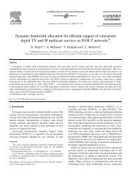
The corresponding functions <strong>for</strong> the other <strong>for</strong>warding<br />
areas are calculated analogously. In Fig. 7, the expected<br />
progress Eðmax i#nX iÞ is shown depending on the number of<br />
nodes located in the <strong>for</strong>warding area. As expected the<br />
progress of the sector is higher than <strong>for</strong> the Reuleaux<br />
triangle and the circle since the center of gravity is located<br />
farther away from the previous node. However, the different<br />
sizes of the <strong>for</strong>warding areas are not taken into account.<br />
From (4) and (8), we obtain the following function <strong>for</strong> the<br />
expected progress P; which takes into account the node<br />
Fig. 7. Expected progress vs. number of nodes.<br />
M. Heissenbüttel et al. / Computer Communications 27 (2004) 1076–1086 1083<br />
ð7Þ<br />
density n:<br />
P < X1<br />
k¼1<br />
rffiffiffiffiffiffiffi<br />
p<br />
¼ pffiffiffi<br />
12<br />
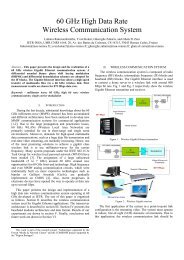
Fig. 8. Expected progress vs. number of neighbors.<br />
e 2nA FðrÞ ðnA FðrÞÞ k<br />
k!<br />
e 2nA FðrÞ X1<br />
k¼1<br />
rffiffiffiffiffiffiffi<br />
p 2k<br />
pffiffiffi<br />
12 2k þ 1<br />
ðnA FðrÞÞ k<br />
k!<br />
2k<br />
2k þ 1<br />
In Fig. 8, the expected progress P is shown as a function<br />
of the number of neighbors of a node, which is directly<br />
related to the overall node density and the transmission<br />
range r: The progress is almost the same <strong>for</strong> all <strong>for</strong>warding<br />
areas, independent of the actual number of neighbors.<br />
There<strong>for</strong>e we may conclude that the best choice <strong>for</strong> the<br />
<strong>for</strong>warding area is the circle since it gives about the same<br />
progress per hop as the other two <strong>for</strong>warding areas,<br />
independent of the actual node density, and at the same<br />
time gives by far the highest number of successful hops<br />
be<strong>for</strong>e the greedy mode fails (cp. Fig. 4).<br />
5. Per<strong>for</strong>mance considerations<br />
In this section, the concept of <strong>BLR</strong> is verified through<br />
simulations. We compare the per<strong>for</strong>mance of <strong>BLR</strong> to the<br />
well-known GPSR [12] and LAR1 [13] protocols. The<br />
protocols are implemented in QualNet [46], a discrete-event<br />
network simulator that includes detailed models <strong>for</strong> wire<strong>less</strong><br />
networking. The following scenarios are configured <strong>for</strong> the<br />
per<strong>for</strong>mance evaluation. 200 nodes are randomly placed<br />
over a 600 £ 3000 m 2 flat terrain where the simulation lasts<br />
<strong>for</strong> 900 s. The rectangular shape of the simulation area is<br />
chosen to obtain longer paths, i.e. a higher average hop<br />
count. The random waypoint mobility model is applied<br />
where the speed of the nodes is randomly chosen between 1<br />
and 40 m=s: (cp. [47]). There is one Constant Bit Rate (CBR)<br />
source which generates two 64 byte UDP packets each<br />
second. The source and destination node of the CBR flow<br />
are randomly chosen among all 200 nodes. The traffic starts