Introduction to AI Robotics.pdf
Introduction to AI Robotics.pdf
Introduction to AI Robotics.pdf

You also want an ePaper? Increase the reach of your titles
YUMPU automatically turns print PDFs into web optimized ePapers that Google loves.
I N T R O D U C T I O N T O<br />
<strong>AI</strong> ROBOTICS<br />
ROBIN R. MURPHY
<strong>Introduction</strong><br />
<strong>to</strong><br />
<strong>AI</strong><br />
<strong>Robotics</strong>
Intelligent Robots and Au<strong>to</strong>nomous Agents<br />
Ronald C. Arkin, edi<strong>to</strong>r<br />
Behavior-Based <strong>Robotics</strong>, Ronald C. Arkin, 1998<br />
Robot Shaping: An Experiment in Behavior Engineering, Marco Dorigo and Marco<br />
Colombetti, 1998<br />
Layered Learning in Multiagent Systems: A Winning Approach <strong>to</strong> Robotic Soccer,<br />
Peter S<strong>to</strong>ne, 2000<br />
Evolutionary <strong>Robotics</strong>: The Biology, Intelligence, and Technology of Self-Organizing<br />
Machines, Stefano Nolfi and Dario Floreano, 2000<br />
Reasoning about Rational Agents, Michael Wooldridge, 2000<br />
<strong>Introduction</strong> <strong>to</strong> <strong>AI</strong> <strong>Robotics</strong>, Robin R. Murphy, 2000
<strong>Introduction</strong><br />
<strong>to</strong><br />
<strong>AI</strong><br />
<strong>Robotics</strong><br />
Robin R. Murphy<br />
ABradfordBook<br />
The MIT Press<br />
Cambridge, Massachusetts<br />
London, England
© 2000 Massachusetts Institute of Technology<br />
All rights reserved. No part of this book may be reproduced in any form by any<br />
electronic or mechanical means (including pho<strong>to</strong>copying, recording, or information<br />
s<strong>to</strong>rage and retrieval) without permission in writing from the publisher.<br />
Typeset in 10/13 Lucida Bright by the author using L ATEX2".<br />
Printed and bound in the United States of America.<br />
Library of Congress Cataloging-in-Publication Data<br />
Murphy, Robin, 1957–<br />
<strong>Introduction</strong> <strong>to</strong> <strong>AI</strong> robotics / Robin R. Murphy.<br />
p. cm.—(Intelligent robotics and au<strong>to</strong>nomous agents. A Bradford Book.)<br />
Includes bibliographical references and index.<br />
ISBN 0-262-13383-0 (hc. : alk. paper)<br />
1. <strong>Robotics</strong>. 2. Artificial intelligence. I. Title. II. Series<br />
TJ211.M865 2000<br />
629.8 0<br />
6263—dc21 00-033251
To Kevin<br />
...andCarlyleRamsey,MonroeSwilley, Chris Trowell<br />
v
Brief Contents<br />
I Robotic Paradigms 1<br />
1 From Teleoperation To Au<strong>to</strong>nomy 13<br />
2 The Hierarchical Paradigm 41<br />
3 Biological Foundations of the Reactive Paradigm 67<br />
4 The Reactive Paradigm 105<br />
5 Designing a Reactive Implementation 155<br />
6 Common Sensing Techniques for Reactive Robots 195<br />
7 The Hybrid Deliberative/Reactive Paradigm 257<br />
8 Multi-agents 293<br />
II Navigation 315<br />
9 Topological Path Planning 325<br />
10 Metric Path Planning 351<br />
11 Localization and Map Making 375<br />
12 On the Horizon 435
Contents<br />
Preface xvii<br />
I Robotic Paradigms 1<br />
1 From Teleoperation To Au<strong>to</strong>nomy 13<br />
1.1 Overview 13<br />
1.2 How Can a Machine Be Intelligent? 15<br />
1.3 What Can Robots Be Used For? 16<br />
1.3.1 Social implications of robotics 18<br />
1.4 A Brief His<strong>to</strong>ry of <strong>Robotics</strong> 19<br />
1.4.1 Industrial manipula<strong>to</strong>rs 21<br />
1.4.2 Space robotics and the <strong>AI</strong> approach 26<br />
1.5 Teleoperation 28<br />
1.5.1 Telepresence 32<br />
1.5.2 Semi-au<strong>to</strong>nomous control 33<br />
1.6 The Seven Areas of <strong>AI</strong> 34<br />
1.7 Summary 37<br />
1.8 Exercises 37<br />
1.9 End Notes 39<br />
2 The Hierarchical Paradigm 41<br />
2.1 Overview 41<br />
2.2 Attributes of the Hierarchical Paradigm 42<br />
2.2.1 Strips 44<br />
2.2.2 More realistic Strips example 46<br />
2.2.3 Strips summary 52
x Contents<br />
2.3 Closed World Assumption and the Frame Problem 53<br />
2.4 Representative Architectures 54<br />
2.4.1 Nested Hierarchical Controller 54<br />
2.4.2 NIST RCS 57<br />
2.4.3 Evaluation of hierarchical architectures 59<br />
2.5 Advantages and Disadvantages 61<br />
2.6 Programming Considerations 62<br />
2.7 Summary 62<br />
2.8 Exercises 63<br />
2.9 End Notes 64<br />
3 Biological Foundations of the Reactive Paradigm 67<br />
3.1 Overview 67<br />
3.1.1 Why explore the biological sciences? 69<br />
3.1.2 Agency and computational theory 70<br />
3.2 What Are Animal Behaviors? 73<br />
3.2.1 Reflexive behaviors 74<br />
3.3 Coordination and Control of Behaviors 75<br />
3.3.1 Innate releasing mechanisms 77<br />
3.3.2 Concurrent behaviors 82<br />
3.4 Perception in Behaviors 83<br />
3.4.1 Action-perception cycle 83<br />
3.4.2 Two functions of perception 85<br />
3.4.3 Gibson: Ecological approach 85<br />
3.4.4 Neisser: Two perceptual systems 90<br />
3.5 Schema Theory 91<br />
3.5.1 Behaviors and schema theory 92<br />
3.6 Principles and Issues in Transferring Insights <strong>to</strong> Robots 97<br />
3.7 Summary 99<br />
3.8 Exercises 100<br />
3.9 End Notes 102<br />
4 The Reactive Paradigm 105<br />
4.1 Overview 105<br />
4.2 Attributes of Reactive Paradigm 108<br />
4.2.1 Characteristics and connotations of reactive<br />
behaviors 110<br />
4.2.2 Advantages of programming by behavior 112<br />
4.2.3 Representative architectures 113
Contents xi<br />
4.3 Subsumption Architecture 113<br />
4.3.1 Example 115<br />
4.3.2 Subsumption summary 121<br />
4.4 Potential Fields Methodologies 122<br />
4.4.1 Visualizing potential fields 123<br />
4.4.2 Magnitude profiles 126<br />
4.4.3 Potential fields and perception 128<br />
4.4.4 Programming a single potential field 129<br />
4.4.5 Combination of fields and behaviors 130<br />
4.4.6 Example using one behavior per sensor 134<br />
4.4.7 Pfields compared with subsumption 136<br />
4.4.8 Advantages and disadvantages 145<br />
4.5 Evaluation of Reactive Architectures 147<br />
4.6 Summary 148<br />
4.7 Exercises 149<br />
4.8 End Notes 152<br />
5 Designing a Reactive Implementation 155<br />
5.1 Overview 155<br />
5.2 Behaviors as Objects in OOP 157<br />
5.2.1 Example: A primitive move-<strong>to</strong>-goal behavior 158<br />
5.2.2 Example: An abstract follow-corridor behavior 160<br />
5.2.3 Where do releasers go in OOP? 162<br />
5.3 Steps in Designing a Reactive Behavioral System 163<br />
5.4 Case Study: Unmanned Ground <strong>Robotics</strong> Competition 165<br />
5.5 Assemblages of Behaviors 173<br />
5.5.1 Finite state au<strong>to</strong>mata 174<br />
5.5.2 A Pick Up the Trash FSA 178<br />
5.5.3 Implementation examples 182<br />
5.5.4 Abstract behaviors 184<br />
5.5.5 Scripts 184<br />
5.6 Summary 187<br />
5.7 Exercises 188<br />
5.8 End Notes 191<br />
6 Common Sensing Techniques for Reactive Robots 195<br />
6.1 Overview 196<br />
6.1.1 Logical sensors 197<br />
6.2 Behavioral Sensor Fusion 198
xii Contents<br />
6.3 Designing a Sensor Suite 202<br />
6.3.1 Attributes of a sensor 203<br />
6.3.2 Attributes of a sensor suite 206<br />
6.4 Proprioceptive Sensors 207<br />
6.4.1 Inertial navigation system (INS) 208<br />
6.4.2 GPS 208<br />
6.5 Proximity Sensors 210<br />
6.5.1 Sonar or ultrasonics 210<br />
6.5.2 Infrared (IR) 216<br />
6.5.3 Bump and feeler sensors 217<br />
6.6 Computer Vision 218<br />
6.6.1 CCD cameras 219<br />
6.6.2 Grayscale and color representation 220<br />
6.6.3 Region segmentation 226<br />
6.6.4 Color his<strong>to</strong>gramming 228<br />
6.7 Range from Vision 231<br />
6.7.1 Stereo camera pairs 232<br />
6.7.2 Light stripers 235<br />
6.7.3 Laser ranging 239<br />
6.7.4 Texture 241<br />
6.8 Case Study: Hors d’Oeuvres, Anyone? 242<br />
6.9 Summary 250<br />
6.10 Exercises 251<br />
6.11 End Notes 254<br />
7 The Hybrid Deliberative/Reactive Paradigm 257<br />
7.1 Overview 257<br />
7.2 Attributes of the Hybrid Paradigm 259<br />
7.2.1 Characteristics and connotation of reactive<br />
behaviors in hybrids 261<br />
7.2.2 Connotations of “global” 262<br />
7.3 Architectural Aspects 262<br />
7.3.1 Common components of hybrid architectures 263<br />
7.3.2 Styles of hybrid architectures 264<br />
7.4 Managerial Architectures 265<br />
7.4.1 Au<strong>to</strong>nomous Robot Architecture (AuRA) 265<br />
7.4.2 Sensor Fusion Effects (SFX) 268<br />
7.5 State-Hierarchy Architectures 274<br />
7.5.1 3-Tiered (3T) 274
Contents xiii<br />
7.6 Model-Oriented Architectures 277<br />
7.6.1 Saphira 278<br />
7.6.2 Task Control Architecture (TCA) 280<br />
7.7 Other Robots in the Hybrid Paradigm 283<br />
7.8 Evaluation of Hybrid Architectures 284<br />
7.9 Interleaving Deliberation and Reactive Control 285<br />
7.10 Summary 288<br />
7.11 Exercises 289<br />
7.12 End Notes 291<br />
8 Multi-agents 293<br />
8.1 Overview 293<br />
8.2 Heterogeneity 296<br />
8.2.1 Homogeneous teams and swarms 296<br />
8.2.2 Heterogeneous teams 297<br />
8.2.3 Social entropy 300<br />
8.3 Control 301<br />
8.4 Cooperation 303<br />
8.5 Goals 304<br />
8.6 Emergent Social Behavior 305<br />
8.6.1 Societal rules 305<br />
8.6.2 Motivation 307<br />
8.7 Summary 309<br />
8.8 Exercises 310<br />
8.9 End Notes 312<br />
II Navigation 315<br />
9 Topological Path Planning 325<br />
9.1 Overview 325<br />
9.2 Landmarks and Gateways 326<br />
9.3 Relational Methods 328<br />
9.3.1 Distinctive places 329<br />
9.3.2 Advantages and disadvantages 331<br />
9.4 Associative Methods 333<br />
9.4.1 Visual homing 334<br />
9.4.2 QualNav 335
xiv Contents<br />
9.5 Case Study of Topological Navigation with a<br />
Hybrid Architecture 338<br />
9.5.1 Path planning 339<br />
9.5.2 Navigation scripts 343<br />
9.5.3 Lessons learned 346<br />
9.6 Summary 348<br />
9.7 Exercises 348<br />
9.8 End notes 350<br />
10 Metric Path Planning 351<br />
10.1 Objectives and Overview 351<br />
10.2 Configuration Space 353<br />
10.3 Cspace Representations 354<br />
10.3.1 Meadow maps 354<br />
10.3.2 Generalized Voronoi graphs 357<br />
10.3.3 Regular grids 358<br />
10.3.4 Quadtrees 359<br />
10.4 Graph Based Planners 359<br />
10.5 Wavefront Based Planners 365<br />
10.6 Interleaving Path Planning and Reactive Execution 367<br />
10.7 Summary 371<br />
10.8 Exercises 372<br />
10.9 End Notes 374<br />
11 Localization and Map Making 375<br />
11.1 Overview 375<br />
11.2 Sonar Sensor Model 378<br />
11.3 Bayesian 380<br />
11.3.1 Conditional probabilities 381<br />
11.3.2 Conditional probabilities for P (Hjs) 384<br />
11.3.3 Updating with Bayes’ rule 385<br />
11.4 Dempster-Shafer Theory 386<br />
11.4.1 Shafer belief functions 387<br />
11.4.2 Belief function for sonar 389<br />
11.4.3 Dempster’s rule of combination 390<br />
11.4.4 Weight of conflict metric 394<br />
11.5 HIMM 395<br />
11.5.1 HIMM sonar model and updating rule 395<br />
11.5.2 Growth rate opera<strong>to</strong>r 398
Contents xv<br />
11.6 Comparison of Methods 403<br />
11.6.1 Example computations 403<br />
11.6.2 Performance 411<br />
11.6.3 Errors due <strong>to</strong> observations from stationary robot 412<br />
11.6.4 Tuning 413<br />
11.7 Localization 415<br />
11.7.1 Continuous localization and mapping 416<br />
11.7.2 Feature-based localization 421<br />
11.8 Exploration 424<br />
11.8.1 Frontier-based exploration 425<br />
11.8.2 Generalized Voronoi graph methods 427<br />
11.9 Summary 428<br />
11.10 Exercises 431<br />
11.11 End Notes 434<br />
12 On the Horizon 435<br />
12.1 Overview 435<br />
12.2 Shape-Shifting and Legged Platforms 438<br />
12.3 Applications and Expectations 442<br />
12.4 Summary 445<br />
12.5 Exercises 445<br />
12.6 End Notes 447<br />
Bibliography 449<br />
Index 459
Preface<br />
This book is intended <strong>to</strong> serve as a textbook for advanced juniors and seniors<br />
and first-year graduate students in computer science and engineering. The<br />
reader is not expected <strong>to</strong> have taken a course in artificial intelligence (<strong>AI</strong>),<br />
although the book includes pointers <strong>to</strong> additional readings and advanced<br />
exercises for more advanced students. The reader should have had at least<br />
one course in object-oriented programming in order <strong>to</strong> follow the discussions<br />
on how <strong>to</strong> implement and program robots using the structures described in<br />
this book. These programming structures lend themselves well <strong>to</strong> labora<strong>to</strong>ry<br />
exercises on commercially available robots, such as the Khepera, Nomad 200<br />
series, and Pioneers. Lego Minds<strong>to</strong>rms and Rug Warrior robots can be used<br />
for the first six chapters, but their current programming interface and sensor<br />
limitations interfere with using those robots for the more advanced material.<br />
A background in digital circuitry is not required, although many instruc<strong>to</strong>rs<br />
may want <strong>to</strong> introduce labora<strong>to</strong>ry exercises for building reactive robots from<br />
kits such as the Rug Warrior or the Handy Board.<br />
<strong>Introduction</strong> <strong>to</strong> <strong>AI</strong> <strong>Robotics</strong> attempts <strong>to</strong> cover all the <strong>to</strong>pics needed <strong>to</strong> program<br />
an artificially intelligent robot for applications involving sensing, navigation,<br />
path planning, and navigating with uncertainty. Although machine<br />
perception is a separate field of endeavor, the book covers enough computer<br />
vision and sensing <strong>to</strong> enable students <strong>to</strong> embark on a serious robot project<br />
or competition. The book is divided in<strong>to</strong> two parts. Part I defines what are<br />
intelligent robots and introduces why artificial intelligence is needed. It covers<br />
the “theory” of <strong>AI</strong> robotics, taking the reader through a his<strong>to</strong>rical journey<br />
from the Hierarchical <strong>to</strong> the Hybrid Deliberative/Reactive Paradigm for organizing<br />
intelligence. The bulk of the seven chapters is concerned with the<br />
Reactive Paradigm and behaviors. A chapter on sensing and programming<br />
techniques for reactive behaviors is included in order <strong>to</strong> permit a class <strong>to</strong> get
xviii Preface<br />
a head start on a programming project. Also, Part I covers the coordination<br />
and control of teams of multi-agents. Since the fundamental mission of a<br />
mobile robot involves moving about in the world, Part II devotes three chapters<br />
<strong>to</strong> qualitative and metric navigation and path planning techniques, plus<br />
work in uncertainty management. The book concludes with an overview of<br />
how advances in computer vision are now being integrated in<strong>to</strong> robots, and<br />
how successes in robots are driving the web-bot and know-bot craze.<br />
Since <strong>Introduction</strong> <strong>to</strong> <strong>AI</strong> <strong>Robotics</strong> is an introduc<strong>to</strong>ry text, it is impossible <strong>to</strong><br />
cover all the fine work that has been in the field. The guiding principle has<br />
been <strong>to</strong> include only material that clearly illuminates a specific <strong>to</strong>pic. References<br />
<strong>to</strong> other approaches and systems are usually included as an advanced<br />
reading question at the end of the chapter or as an end note. Behavior-based<br />
<strong>Robotics</strong> 10 provides a thorough survey of the field and should be an instruc<strong>to</strong>r’s<br />
companion.<br />
Acknowledgments<br />
It would be impossible <strong>to</strong> thank all of the people involved in making this<br />
book possible, but I would like <strong>to</strong> try <strong>to</strong> list the ones who made the most<br />
obvious contributions. I’d like <strong>to</strong> thank my parents (I think this is the equivalent<br />
of scoring a goal and saying “Hi Mom!” on national TV) and my family<br />
(Kevin, Kate, and Allan). I had the honor of being in the first <strong>AI</strong> robotics<br />
course taught by my PhD advisor Ron Arkin at Georgia Tech (where I was<br />
also his first PhD student), and much of the material and organization of this<br />
book can be traced back <strong>to</strong> his course. I have tried <strong>to</strong> maintain the intellectual<br />
rigor of his course and excellent book while trying <strong>to</strong> distill the material<br />
for a novice audience. Any errors in this book are strictly mine. David Kortenkamp<br />
suggested that I write this book after using my course notes for a<br />
class he taught, which served as a very real catalyst. Certainly the students<br />
at both the Colorado School of Mines (CSM), where I first developed my<br />
robotics courses, and at the University of South Florida (USF) merit special<br />
thanks for being guinea pigs. I would like <strong>to</strong> specifically thank Leslie Baski,<br />
John Blitch, Glenn Blauvelt, Ann Brigante, Greg Chavez, Aaron Gage, Dale<br />
Hawkins, Floyd Henning, Jim Hoffman, Dave Hershberger, Kevin Gifford,<br />
Matt Long, Charlie Ozinga, Tonya Reed Frazier, Michael Rosenblatt, Jake<br />
Sprouse, Brent Taylor, and Paul Wiebe from my CSM days and Jenn Casper,<br />
Aaron Gage, Jeff Hyams, Liam Irish, Mark Micire, Brian Minten, and Mark<br />
Powell from USF.
Preface xix<br />
Special thanks go <strong>to</strong> the numerous reviewers, especially Karen Sutherland<br />
and Ken Hughes. Karen Sutherland and her robotics class at the University<br />
of Wisconsin-LaCrosse (Kris<strong>to</strong>ff Hans Ausderau, Teddy Bauer, Scott David<br />
Becker, Corrie L. Brague, Shane Brownell, Edwin J. Colby III, Mark Erickson,<br />
Chris Falch, Jim Fick, Jennifer Fleischman, Scott Galbari, Mike Halda,<br />
Brian Kehoe, Jay D. Paska, Stephen Pauls, Scott Sandau, Amy Stanislowski,<br />
Jaromy Ward, Steve Westcott, Peter White, Louis Woyak, and Julie A. Zander)<br />
painstakingly reviewed an early draft of the book and made extensive<br />
suggestions and added review questions. Ken Hughes also deserves special<br />
thanks; he also provided a chapter by chapter critique as well as witty emails.<br />
Ken always comes <strong>to</strong> my rescue.<br />
Likewise, the book would not be possible without my ongoing involvement<br />
in robotics research; my efforts have been supported by NSF, DARPA,<br />
and ONR. Most of the case studies came from work or through equipment<br />
sponsored by NSF. Howard Moraff, Rita Rodriguez, and Harry Hedges were<br />
always very encouraging, beyond the call of duty of even the most dedicated<br />
NSF program direc<strong>to</strong>r. Michael Mason also provided encouragement,<br />
in many forms, <strong>to</strong> hang in there and focus on education.<br />
My edi<strong>to</strong>r, Bob Prior, and the others at the MIT Press (Katherine Innis,<br />
Judy Feldmann, Margie Hardwick, and Maureen Kuper) also have my deepest<br />
appreciation for providing unfailingly good-humored guidance, technical<br />
assistance, and general savvy. Katherine and especially Judy were very<br />
patient and nice— despite knowing that I was calling with Yet Another Crisis.<br />
Mike Hamil<strong>to</strong>n at AA<strong>AI</strong> was very helpful in making available the various<br />
“action shots” used throughout the book. Chris Manning provided the<br />
L ATEX2"style files, with adaptations by Paul Anagnos<strong>to</strong>poulos. Liam Irish<br />
and Ken Hughes contributed helpful scripts.<br />
Besides the usual suspects, there are some very special people who indirectly<br />
helped me. Without the encouragement of three liberal arts professors,<br />
Carlyle Ramsey, Monroe Swilley, and Chris Trowell, at South Georgia College<br />
in my small home<strong>to</strong>wn of Douglas, Georgia, I probably wouldn’t have<br />
seriously considered graduate school in engineering and computer science.<br />
They taught me that learning isn’t a place like a big university but rather a<br />
personal discipline. The efforts of my husband, Kevin Murphy, were, as always,<br />
essential. He worked hard <strong>to</strong> make sure I could spend the time on this<br />
book without missing time with the kids or going crazy. He also did a serious<br />
amount of editing, typing, scanning, and proofreading. I dedicate the<br />
book <strong>to</strong> these four men who have influenced my professional career as much<br />
as any academic men<strong>to</strong>r.
P ART I<br />
Robotic Paradigms
2 Part I<br />
Contents:<br />
Overview<br />
Chapter 1: From Teleoperation <strong>to</strong> Au<strong>to</strong>nomy<br />
Chapter 2: The Hierarchical Paradigm<br />
Chapter 3: Biological Foundations of the Reactive Paradigm<br />
Chapter 4: The Reactive Paradigm<br />
Chapter 5: Designing a Reactive Implementation<br />
Chapter 6: Common Sensing Technique for Reactive Robots<br />
Chapter 7: The Hybrid Deliberative/Reactive Paradigm<br />
Chapter 8: Multiple Mobile Robots<br />
Overview<br />
The eight chapters in this part are devoted <strong>to</strong> describing what is <strong>AI</strong> robotics<br />
and the three major paradigms for achieving it. These paradigms characterize<br />
the ways in which intelligence is organized in robots. This part of the<br />
book also covers architectures that provide exemplars of how <strong>to</strong> transfer the<br />
principles of the paradigm in<strong>to</strong> a coherent, reusable implementation on a<br />
single robot or teams of robots.<br />
What Are Robots?<br />
One of the first questions most people have about robotics is “what is a robot?”<br />
followed immediately by “what can they do?”<br />
In popular culture, the term “robot” generally connotes some anthropomorphic<br />
(human-like) appearance; consider robot “arms” for welding. The<br />
tendency <strong>to</strong> think about robots as having a human-like appearance may stem<br />
from the origins of the term “robot.” The word “robot” came in<strong>to</strong> the popular<br />
consciousness on January 25, 1921, in Prague with the first performance<br />
of Karel Capek’s play, R.U.R. (Rossum’s Universal Robots). 37 In R.U.R., an<br />
unseen inven<strong>to</strong>r, Rossum, has created a race of workers made from a vat of<br />
biological parts, smart enough <strong>to</strong> replace a human in any job (hence “universal”).<br />
Capek described the workers as robots, a term derived from the Czech
INTELLIGENT ROBOT<br />
Part I 3<br />
word “robota” which is loosely translated as menial laborer. Robot workers<br />
implied that the artificial creatures were strictly meant <strong>to</strong> be servants <strong>to</strong> free<br />
“real” people from any type of labor, but were <strong>to</strong>o lowly <strong>to</strong> merit respect.<br />
This attitude <strong>to</strong>wards robots has disastrous consequences, and the moral of<br />
the rather socialist s<strong>to</strong>ry is that work defines a person.<br />
The shift from robots as human-like servants constructed from biological<br />
parts <strong>to</strong> human-like servants made up of mechanical parts was probably due<br />
<strong>to</strong> science fiction. Three classic films, Metropolis (1926), TheDaytheEarth<br />
S<strong>to</strong>od Still (1951), and Forbidden Planet (1956), cemented the connotation that<br />
robots were mechanical in origin, ignoring the biological origins in Capek’s<br />
play. Meanwhile, computers were becoming commonplace in industry and<br />
accounting, gaining a perception of being literal minded. Industrial au<strong>to</strong>mation<br />
confirmed this suspicion as robot arms were installed which would go<br />
through the motions of assembling parts, even if there were no parts. Eventually,<br />
the term robot <strong>to</strong>ok on nuances of fac<strong>to</strong>ry au<strong>to</strong>mation: mindlessness<br />
and good only for well-defined repetitious types of work. The notion of<br />
anthropomorphic, mechanical, and literal-minded robots complemented the<br />
viewpoint taken in many of the short s<strong>to</strong>ries in Isaac Asimov’s perennial favorite<br />
collection, I, Robot. 15 Many (but not all) of these s<strong>to</strong>ries involve either<br />
a “robopsychologist,” Dr. Susan Calvin, or two erstwhile trouble shooters,<br />
Powell and Donovan, diagnosing robots who behaved logically but did the<br />
wrong thing.<br />
The shift from human-like mechanical creatures <strong>to</strong> whatever shape gets<br />
the job done is due <strong>to</strong> reality. While robots are mechanical, they don’t have <strong>to</strong><br />
be anthropomorphic or even animal-like. Consider robot vacuum cleaners;<br />
they look like vacuum cleaners, not jani<strong>to</strong>rs. And the HelpMate <strong>Robotics</strong>,<br />
Inc., robot which delivers hospital meals <strong>to</strong> patients <strong>to</strong> permit nurses more<br />
time with patients, looks like a cart, not a nurse.<br />
It should be clear from Fig. I.1 that appearance does not form a useful definition<br />
of a robot. Therefore, the definition that will be used in this book<br />
is an intelligent robot is a mechanical creature which can function au<strong>to</strong>nomously.<br />
“Intelligent” implies that the robot does not do things in a mindless, repetitive<br />
way; it is the opposite of the connotation from fac<strong>to</strong>ry au<strong>to</strong>mation. The<br />
“mechanical creature” portion of the definition is an acknowledgment of the<br />
fact that our scientific technology uses mechanical building blocks, not biological<br />
components (although with recent advances in cloning, this may<br />
change). It also emphasizes that a robot is not the same as a computer. A robot<br />
may use a computer as a building block, equivalent <strong>to</strong> a nervous system<br />
or brain, but the robot is able <strong>to</strong> interact with its world: move around, change
4 Part I<br />
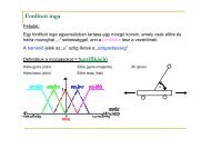
a. b.<br />
Figure I.1 Two views of robots: a) the humanoid robot from the 1926 movie<br />
Metropolis (image courtesty Fr. Doug Quinn and the Metropolis Home<br />
Page), and b) a HMMWV military vehicle capable of driving on roads and<br />
open terrains. (Pho<strong>to</strong>graph courtesy of the National Institute for Standards<br />
and Technology.)<br />
it, etc. A computer doesn’t move around under its own power. “Function<br />
au<strong>to</strong>nomously” indicates that the robot can operate, self-contained, under<br />
all reasonable conditions without requiring recourse <strong>to</strong> a human opera<strong>to</strong>r.<br />
Au<strong>to</strong>nomy means that a robot can adapt <strong>to</strong> changes in its environment (the<br />
lights get turned off) or itself (a part breaks) and continue <strong>to</strong> reach its goal.<br />
Perhaps the best example of an intelligent mechanical creature which can<br />
function au<strong>to</strong>nomously is the Termina<strong>to</strong>r from the 1984 movie of the same<br />
name. Even after losing one camera (eye) and having all external coverings<br />
(skin, flesh) burned off, it continued <strong>to</strong> pursue its target (Sarah Connor).<br />
Extreme adaptability and au<strong>to</strong>nomy in an extremely scary robot! A more<br />
practical (and real) example is Marvin, the mail cart robot, for the Baltimore<br />
FBI office, described in a Nov. 9, 1996, article in the Denver Post. Marvin is<br />
able <strong>to</strong> accomplish its goal of s<strong>to</strong>pping and delivering mail while adapting<br />
<strong>to</strong> people getting in its way at unpredictable times and locations.
PARADIGM<br />
ROBOTIC PARADIGMS<br />
Part I 5<br />
What are Robotic Paradigms?<br />
A paradigm is a philosophy or set of assumptions and/or techniques which characterize<br />
an approach <strong>to</strong> a class of problems. It is both a way of looking at the world<br />
and an implied set of <strong>to</strong>ols for solving problems. No one paradigm is right;<br />
rather, some problems seem better suited for different approaches. For example,<br />
consider calculus problems. There are problems that could be solved<br />
by differentiating in cartesian (X� Y� Z) coordinates, but are much easier <strong>to</strong><br />
solve if polar coordinates (r� ) are used. In the domain of calculus problems,<br />
Cartesian and polar coordinates represent two different paradigms for viewing<br />
and manipulating a problem. Both produce the correct answer, but one<br />
takes less work for certain problems.<br />
Applying the right paradigm makes problem solving easier. Therefore,<br />
knowing the paradigms of <strong>AI</strong> robotics is one key <strong>to</strong> being able <strong>to</strong> successfully<br />
program a robot for a particular application. It is also interesting from a his<strong>to</strong>rical<br />
perspective <strong>to</strong> work through the different paradigms, and <strong>to</strong> examine<br />
the issues that spawned the shift from one paradigm <strong>to</strong> another.<br />
There are currently three paradigms for organizing intelligence in robots:<br />
hierarchical, reactive, and hybrid deliberative/reactive. The paradigms are<br />
described in two ways.<br />
1. By the relationship between the three commonly accepted primitives<br />
of robotics: SENSE, PLAN, ACT. The functions of a robot can be divided<br />
PRIMITIVES in<strong>to</strong> three very general categories. If a function is taking in information<br />
from the robot’s sensors and producing an output useful by other functions,<br />
then that function falls in the SENSE category. If the function is<br />
taking in information (either from sensors or its own knowledge about<br />
how the world works) and producing one or more tasks for the robot <strong>to</strong><br />
perform (go down the hall, turn left, proceed 3 meters and s<strong>to</strong>p), that function<br />
is in the PLAN category. Functions which produce output commands<br />
<strong>to</strong> mo<strong>to</strong>r actua<strong>to</strong>rs fall in<strong>to</strong> ACT (turn 98 , clockwise, with a turning velocity<br />
of 0.2mps). Fig. I.2 attempts <strong>to</strong> define these three primitives in terms<br />
of inputs and outputs; this figure will appear throughout the chapters in<br />
Part I.<br />
ROBOT PARADIGM<br />
2. By the way sensory data is processed and distributed through the system.<br />
How much a person or robot or animal is influenced by what it<br />
senses. So it is often difficult <strong>to</strong> adequately describe a paradigm with just<br />
a box labeled SENSE. In some paradigms, sensor information is restricted<br />
<strong>to</strong> being used in a specific, or dedicated, way for each function of a robot;
6 Part I<br />
SENSING<br />
ORGANIZATION IN<br />
ROBOT PARADIGMS<br />
ROBOT PRIMITIVES INPUT OUTPUT<br />
SENSE<br />
PLAN<br />
ACT<br />
Sensor data Sensed information<br />
Information (sensed<br />
and/or cognitive)<br />
Sensed information<br />
or directives<br />
Directives<br />
Actua<strong>to</strong>r commands<br />
Figure I.2 Robot primitives defined in terms of inputs and outputs.<br />
in that case processing is local <strong>to</strong> each function. Other paradigms expect<br />
all sensor information <strong>to</strong> be first processed in<strong>to</strong> one global world model<br />
and then subsets of the model distributed <strong>to</strong> other functions as needed.<br />
Overview of the Three Paradigms<br />
In order <strong>to</strong> set the stage for learning details, it may be helpful <strong>to</strong> begin with<br />
a general overview of the robot paradigms. Fig. I.3 shows the differences<br />
between the three paradigms in terms of the SENSE, PLAN, ACT primitives.<br />
The Hierarchical Paradigm is the oldest paradigm, and was prevalent from<br />
PARADIGM 1967–1990. Under it, the robot operates in a <strong>to</strong>p-down fashion, heavy on<br />
planning (see Fig. I.3). This was based on an introspective view of how people<br />
think. “I see a door, I decide <strong>to</strong> head <strong>to</strong>ward it, and I plot a course around<br />
the chairs.” (Unfortunately, as many cognitive psychologists now know, introspection<br />
is not always a good way of getting an accurate assessment of<br />
a thought process. We now suspect no one actually plans how they get out<br />
of a room; they have default schemas or behaviors.) Under the Hierarchical<br />
Paradigm, the robot senses the world, plans the next action, and then acts<br />
(SENSE, PLAN, ACT). Then it senses the world, plans, acts. At each step,<br />
the robot explicitly plans the next move. The other distinguishing feature of<br />
the Hierarchical paradigm is that all the sensing data tends <strong>to</strong> be gathered<br />
in<strong>to</strong> one global world model, a single representation that the planner can use<br />
and can be routed <strong>to</strong> the actions. Constructing generic global world models<br />
HIERARCHICAL
Part I 7<br />
SENSE PLAN ACT<br />
a.<br />
PLAN<br />
SENSE ACT<br />
ACT<br />
b.<br />
PLAN<br />
c.<br />
SENSE<br />
Figure I.3 Three paradigms: a.) Hierarchical, b.) Reactive, and c.) Hybrid<br />
deliberative/reactive.<br />
turns out <strong>to</strong> be very hard and brittle due <strong>to</strong> the frame problem and the need<br />
for a closed world assumption.<br />
Fig. I.4 shows how the Hierarchical Paradigm can be thought of as a transitive,<br />
or Z-like, flow of events through the primitives given in Fig. I.4. Unfortunately,<br />
the flow of events ignored biological evidence that sensed information<br />
can be directly coupled <strong>to</strong> an action, which is why the sensed information<br />
input is blacked out.
8 Part I<br />
REACTIVE PARADIGM<br />
ROBOT PRIMITIVES INPUT OUTPUT<br />
SENSE<br />
PLAN<br />
ACT<br />
Sensor data Sensed information<br />
Information (sensed<br />
and/or cognitive)<br />
Sensed information<br />
or directives<br />
Figure I.4 Another view of the Hierarchical Paradigm.<br />
Directives<br />
Actua<strong>to</strong>r commands<br />
The Reactive Paradigm was a reaction <strong>to</strong> the Hierarchical Paradigm, and<br />
led <strong>to</strong> exciting advances in robotics. It was heavily used in robotics starting<br />
in 1988 and continuing through 1992. It is still used, but since 1992 there<br />
has been a tendency <strong>to</strong>ward hybrid architectures. The Reactive Paradigm<br />
was made possible by two trends. One was a popular movement among <strong>AI</strong><br />
researchers <strong>to</strong> investigate biology and cognitive psychology in order <strong>to</strong> examine<br />
living exemplars of intelligence. Another was the rapidly decreasing<br />
cost of computer hardware coupled with the increase in computing power.<br />
As a result, researchers could emulate frog and insect behavior with robots<br />
costing less than $500 versus the $100,000s Shakey, the first mobile robot,<br />
cost.<br />
The Reactive Paradigm threw out planning all <strong>to</strong>gether (see Figs. I.3b and<br />
I.5). It is a SENSE-ACT (S-A) type of organization. Whereas the Hierarchical<br />
Paradigm assumes that the input <strong>to</strong> a ACT will always be the result of a<br />
PLAN, the Reactive Paradigm assumes that the input <strong>to</strong> an ACT will always<br />
be the direct output of a sensor, SENSE.<br />
If the sensor is directly connected <strong>to</strong> the action, why isn’t a robot running<br />
under the Reactive Paradigm limited <strong>to</strong> doing just one thing? The robot has<br />
multiple instances of SENSE-ACT couplings, discussed in Ch. 4. These couplings<br />
are concurrent processes, called behaviors, which take local sensing<br />
data and compute the best action <strong>to</strong> take independently of what the other<br />
processes are doing. One behavior can direct the robot <strong>to</strong> “move forward 5<br />
meters” (ACT on drive mo<strong>to</strong>rs) <strong>to</strong> reach a goal (SENSE the goal), while another<br />
behavior can say “turn 90 ”(ACT on steer mo<strong>to</strong>rs) <strong>to</strong> avoid a collision
HYBRID DELIBERA-<br />
TIVE/REACTIVE<br />
PARADIGM<br />
Part I 9<br />
ROBOT PRIMITIVES INPUT OUTPUT<br />
SENSE<br />
PLAN<br />
ACT<br />
Figure I.5 The reactive paradigm.<br />
Sensor data Sensed information<br />
Information (sensed<br />
and/or cognitive)<br />
Sensed information<br />
or directives<br />
Directives<br />
Actua<strong>to</strong>r commands<br />
with an object dead ahead (SENSE obstacles). The robot will do a combination<br />
of both behaviors, swerving off course temporarily at a 45 angle <strong>to</strong><br />
avoid the collision. Note that neither behavior directed the robot <strong>to</strong> ACT with<br />
a 45 turn; the final ACT emerged from the combination of the two behaviors.<br />
While the Reactive Paradigm produced exciting results and clever robot<br />
insect demonstrations, it quickly became clear that throwing away planning<br />
was <strong>to</strong>o extreme for general purpose robots. In some regards, the Reactive<br />
Paradigm reflected the work of Harvard psychologist B. F. Skinner in<br />
stimulus-response training with animals. It explained how some animals<br />
accomplished tasks, but was a dead end in explaining the entire range of<br />
human intelligence.<br />
But the Reactive Paradigm has many desirable properties, especially the<br />
fast execution time that came from eliminating any planning. As a result,<br />
the Reactive Paradigm serves as the basis for the Hybrid Deliberative/Reactive<br />
Paradigm, shown in Fig.I.3c. The Hybrid Paradigm emerged in the 1990’s and<br />
continues <strong>to</strong> be the current area of research. Under the Hybrid Paradigm, the<br />
robot first plans (deliberates) how <strong>to</strong> best decompose a task in<strong>to</strong> subtasks<br />
(also called “mission planning”) and then what are the suitable behaviors <strong>to</strong><br />
accomplish each subtask, etc. Then the behaviors start executing as per the<br />
Reactive Paradigm. This type of organization is PLAN, SENSE-ACT (P, S-A),<br />
where the comma indicates that planning is done at one step, then sensing<br />
and acting are done <strong>to</strong>gether. Sensing organization in the Hybrid Paradigm<br />
is also a mixture of Hierarchical and Reactive styles. Sensor data gets routed<br />
<strong>to</strong> each behavior that needs that sensor, but is also available <strong>to</strong> the planner
10 Part I<br />
ARCHITECTURE<br />
ROBOT PRIMITIVES INPUT OUTPUT<br />
PLAN<br />
SENSE-ACT<br />
(behaviors)<br />
Information (sensed<br />
and/or cognitive)<br />
Sensor data<br />
Figure I.6 The hybrid deliberative/reactive paradigm.<br />
Directives<br />
Actua<strong>to</strong>r commands<br />
for construction of a task-oriented global world model. The planner may<br />
also “eavesdrop” on the sensing done by each behavior (i.e., the behavior<br />
identifies obstacles that could then be put in<strong>to</strong> a map of the world by the<br />
planner). Each function performs computations at its own rate; deliberative<br />
planning, which is generally computationally expensive may update every<br />
5 seconds, while the reactive behaviors often execute at 1/60 second. Many<br />
robots run at 80 centimeters per second.<br />
Architectures<br />
Determining that a particular paradigm is well suited for an application is<br />
certainly the first step in constructing the <strong>AI</strong> component of a robot. But that<br />
step is quickly followed with the need <strong>to</strong> use the <strong>to</strong>ols associated with that<br />
paradigm. In order <strong>to</strong> visualize how <strong>to</strong> apply these paradigms <strong>to</strong> real-world<br />
applications, it is helpful <strong>to</strong> examine representative architectures. These architectures<br />
provide templates for an implementation, as well as examples of<br />
what each paradigm really means.<br />
What is an architecture? Arkin offers several definitions in his book, Behavior-Based<br />
Robots. 10 Two of the definitions he cites from other researchers<br />
capture how the term will be used in this book. Following Mataric, 89 an<br />
architecture provides a principled way of organizing a control system. However,<br />
in addition <strong>to</strong> providing structure, it imposes constraints on the way the<br />
control problem can be solved. Following Dean and Wellman, 43 an architecture<br />
describes a set of architectural components and how they interact. This<br />
book is interested in the components common in robot architectures; these<br />
are the basic building blocks for programming a robot. It also is interested in<br />
the principles and rules of thumb for connecting these components <strong>to</strong>gether.
MODULARITY<br />
NICHE TARGETABILITY<br />
PORTABILITY<br />
ROBUSTNESS<br />
Part I 11<br />
To see the importance of an architecture, consider building a house or a<br />
car. There is no “right” design for a house, although most houses share the<br />
same components (kitchens, bathrooms, walls, floors, doors, etc.). Likewise<br />
with designing robots, there can be multiple ways of organizing the components,<br />
even if all the designs follow the same paradigm. This is similar <strong>to</strong> cars<br />
designed by different manufacturers. All internal combustion engine types<br />
of cars have the same basic components, but the cars look different (BMWs<br />
and Jaguars look quite different than Hondas and Fords). The internal combustion<br />
(IC) engine car is a paradigm (as contrasted <strong>to</strong> the paradigm of an<br />
electric car). Within the IC engine car community, the car manufacturers each<br />
have their own architecture. The car manufacturers may make slight modifications<br />
<strong>to</strong> the architecture for sedans, convertibles, sport-utility vehicles,<br />
etc., <strong>to</strong> throw out unnecessary options, but each style of car is a particular<br />
instance of the architecture. The point is: by studying representative robot<br />
architectures and the instances where they were used for a robot application,<br />
we can learn the different ways that the components and <strong>to</strong>ols associated<br />
with a paradigm can be used <strong>to</strong> build an artificially intelligent robot.<br />
Since a major objective in robotics is <strong>to</strong> learn how <strong>to</strong> build them, an important<br />
skill <strong>to</strong> develop is evaluating whether or not a previously developed<br />
architecture (or large chunks of it) will suit the current application. This skill<br />
will save both time spent on re-inventing the wheel and avoid subtle problems<br />
that other people have encountered and solved. Evaluation requires a<br />
set of criteria. The set that will be used in this book is adapted from Behavior-<br />
Based <strong>Robotics</strong>: 10<br />
1. Support for modularity: does it show good software engineering principles?<br />
2. Niche targetability: how well does it work for the intended application?<br />
3. Ease of portability <strong>to</strong> other domains: how well would it work for other<br />
applications or other robots?<br />
4. Robustness: where is the system vulnerable, and how does it try <strong>to</strong> reduce<br />
that vulnerability?<br />
Note that niche targetability and ease of portability are often at odds with<br />
each other. Most of the architectures described in this book were intended <strong>to</strong><br />
be generic, therefore emphasizing portability. The generic structures, however,<br />
often introduce undesirable computational and s<strong>to</strong>rage overhead, so in<br />
practice the designer must make trade-offs.
12 Part I<br />
Layout of the Section<br />
This section is divided in<strong>to</strong> eight chapters, one <strong>to</strong> define robotics and the<br />
other seven <strong>to</strong> intertwine both the theory and practice associated with each<br />
paradigm. Ch. 2 describes the Hierarchical Paradigm and two representative<br />
architectures. Ch. 3 sets the stage for understanding the Reactive Paradigm<br />
by reviewing the key concepts from biology and ethology that served <strong>to</strong> motivate<br />
the shift from Hierarchical <strong>to</strong> Reactive systems. Ch. 4 describes the<br />
Reactive Paradigm and the architectures that originally popularized this approach.<br />
It also offers definitions of primitive robot behaviors. Ch. 5 provides<br />
guidelines and case studies on designing robot behaviors. It also introduces<br />
issues in coordinating and controlling multiple behaviors and the common<br />
techniques for resolving these issues. At this point, the reader should be<br />
almost able <strong>to</strong> design and implement a reactive robot system, either in simulation<br />
or on a real robot. However, the success of a reactive system depends<br />
on the sensing. Ch. 6 discusses simple sonar and computer vision processing<br />
techniques that are commonly used in inexpensive robots. Ch. 7 describes<br />
the Hybrid Deliberative-Reactive Paradigm, concentrating on architectural<br />
trends. Up until this point, the emphasis is <strong>to</strong>wards programming a single<br />
robot. Ch. 8 concludes the section by discussing how the principles of the<br />
three paradigms have been transferred <strong>to</strong> teams of robots.<br />
End Note<br />
Robot paradigm primitives.<br />
While the SENSE, PLAN, ACT primitives are generally accepted, some researchers<br />
are suggesting that a fourth primitive be added, LEARN. There are no formal architectures<br />
at this time which include this, so a true paradigm shift has not yet occurred.
1 From Teleoperation To Au<strong>to</strong>nomy<br />
Chapter Objectives:<br />
Define intelligent robot.<br />
Be able <strong>to</strong> describe at least two differences between <strong>AI</strong> and Engineering<br />
approaches <strong>to</strong> robotics.<br />
Be able <strong>to</strong> describe the difference between telepresence and semi-au<strong>to</strong>nomous<br />
control.<br />
1.1 Overview<br />
Have some feel for the his<strong>to</strong>ry and societal impact of robotics.<br />
This book concentrates on the role of artificial intelligence for robots. At<br />
first, that may appear redundant; aren’t robots intelligent? The short answer<br />
is “no,” most robots currently in industry are not intelligent by any<br />
definition. This chapter attempts <strong>to</strong> distinguish an intelligent robot from a<br />
non-intelligent robot.<br />
The chapter begins with an overview of artificial intelligence and the social<br />
implications of robotics. This is followed with a brief his<strong>to</strong>rical perspective<br />
on the evolution of robots <strong>to</strong>wards intelligence, as shown in Fig. 1.1. One<br />
way of viewing robots is that early on in the 1960’s there was a fork in the<br />
evolutionary path. Robots for manufacturing <strong>to</strong>ok a fork that has focused on<br />
engineering robot arms for manufacturing applications. The key <strong>to</strong> success in<br />
industry was precision and repeatability on the assembly line for mass production,<br />
in effect, industrial engineers wanted <strong>to</strong> au<strong>to</strong>mate the workplace.<br />
Once a robot arm was programmed, it should be able <strong>to</strong> operate for weeks<br />
and months with only minor maintenance. As a result, the emphasis was
14 1 From Teleoperation To Au<strong>to</strong>nomy<br />
telemanipula<strong>to</strong>rs<br />
planetary rovers<br />
manufacturing<br />
vision<br />
1960 1970 1980 1990 2000<br />
Figure 1.1 A timeline showing forks in development of robots.<br />
<strong>AI</strong> <strong>Robotics</strong><br />
telesystems<br />
Industrial<br />
Manipula<strong>to</strong>rs<br />
placed on the mechanical aspects of the robot <strong>to</strong> ensure precision and repeatability<br />
and methods <strong>to</strong> make sure the robot could move precisely and<br />
repeatable, quickly enough <strong>to</strong> make a profit. Because assembly lines were<br />
engineered <strong>to</strong> mass produce a certain product, the robot didn’t have <strong>to</strong> be<br />
able <strong>to</strong> notice any problems. The standards for mass production would make<br />
it more economical <strong>to</strong> devise mechanisms that would ensure parts would be<br />
in the correct place. A robot for au<strong>to</strong>mation could essentially be blind and<br />
senseless.<br />
<strong>Robotics</strong> for the space program <strong>to</strong>ok a different fork, concentrating instead<br />
on highly specialized, one-of-a-kind planetary rovers. Unlike a highly au<strong>to</strong>mated<br />
manufacturing plant, a planetary rover operating on the dark side of<br />
the moon (no radio communication) might run in<strong>to</strong> unexpected situations.<br />
Consider that on Apollo 17, astronaut and geologist Harrison Schmitt found<br />
an orange rock on the moon; an orange rock was <strong>to</strong>tally unexpected. Ideally,<br />
a robot would be able <strong>to</strong> notice something unusual, s<strong>to</strong>p what it was doing<br />
(as long as it didn’t endanger itself) and investigate. Since it couldn’t be preprogrammed<br />
<strong>to</strong> handle all possible contingencies, it had <strong>to</strong> be able <strong>to</strong> notice<br />
its environment and handle any problems that might occur. At a minimum,<br />
a planetary rover had <strong>to</strong> have some source of sensory inputs, some way of<br />
interpreting those inputs, and a way of modifying its actions <strong>to</strong> respond <strong>to</strong><br />
a changing world. And the need <strong>to</strong> sense and adapt <strong>to</strong> a partially unknown<br />
environment is the need for intelligence.<br />
The fork <strong>to</strong>ward <strong>AI</strong> robots has not reached a termination point of truly au<strong>to</strong>nomous,<br />
intelligent robots. In fact, as will be seen in Ch. 2 and 4, it wasn’t<br />
until the late 1980’s that any visible progress <strong>to</strong>ward that end was made. So<br />
what happened when someone had an application for a robot which needed
1.2 How Can a Machine Be Intelligent? 15<br />
real-time adaptability before 1990? In general, the lack of machine intelligence<br />
was compensated by the development of mechanisms which allow a<br />
human <strong>to</strong> control all, or parts, of the robot remotely. These mechanisms are<br />
generally referred <strong>to</strong> under the umbrella term: teleoperation. Teleoperation<br />
can be viewed as the “stuff” in the middle of the two forks. In practice, intelligent<br />
robots such as the Mars Sojourner are controlled with some form of<br />
teleoperation. This chapter will cover the flavors of teleoperation, given their<br />
importance as a stepping s<strong>to</strong>ne <strong>to</strong>wards truly intelligent robots.<br />
The chapter concludes by visiting the issues in <strong>AI</strong>, and argues that <strong>AI</strong> is imperative<br />
for many robotic applications. Teleoperation is simply not sufficient<br />
or desirable as a long term solution. However, it has served as a reasonable<br />
patch.<br />
It is interesting <strong>to</strong> note that the two forks, manufacturing and <strong>AI</strong>, currently<br />
appear <strong>to</strong> be merging. Manufacturing is now shifting <strong>to</strong> a “mass cus<strong>to</strong>mization”<br />
phase, where companies which can economically make short runs of<br />
special order goods are thriving. The pressure is on for industrial robots,<br />
more correctly referred <strong>to</strong> as industrial manipula<strong>to</strong>rs, <strong>to</strong> be rapidly reprogrammed<br />
and more forgiving if a part isn’t placed exactly as expected in its<br />
workspace. As a result, <strong>AI</strong> techniques are migrating <strong>to</strong> industrial manipula<strong>to</strong>rs.<br />
1.2 How Can a Machine Be Intelligent?<br />
ARTIFICIAL The science of making machines act intelligently is usually referred <strong>to</strong> as artifi-<br />
INTELLIGENCE cial intelligence, or <strong>AI</strong> for short. Artificial Intelligence has no commonly accepted<br />
definitions. One of the first textbooks on <strong>AI</strong> defined it as “the study<br />
of ideas that enable computers <strong>to</strong> be intelligent,” 143 which seemed <strong>to</strong> beg the<br />
question. A later textbook was more specific, “<strong>AI</strong> is the attempt <strong>to</strong> get the<br />
computer <strong>to</strong> do things that, for the moment, people are better at.” 120 This<br />
definition is interesting because it implies that once a task is performed successfully<br />
by a computer, then the technique that made it possible is no longer<br />
<strong>AI</strong>, but something mundane. That definition is fairly important <strong>to</strong> a person<br />
researching <strong>AI</strong> methods for robots, because it explains why certain <strong>to</strong>pics<br />
suddenly seem <strong>to</strong> disappear from the <strong>AI</strong> literature: it was perceived as being<br />
solved! Perhaps the most amusing of all <strong>AI</strong> definitions was the slogan for<br />
the now defunct computer company, Thinking Machines, Inc., “... making<br />
machines that will be proud of us.”
16 1 From Teleoperation To Au<strong>to</strong>nomy<br />
THE 3D’S<br />
The term <strong>AI</strong> is controversial, and has sparked ongoing philosophical debates<br />
on whether a machine can ever be intelligent. As Roger Penrose notes<br />
in his book, The Emperor’s New Mind: “Nevertheless, it would be fair <strong>to</strong><br />
say that, although many clever things have indeed been done, the simulation<br />
of anything that could pass for genuine intelligence is yet a long way<br />
off.“ 115 Engineers often dismiss <strong>AI</strong> as wild speculation. As a result of such<br />
vehement criticisms, many researchers often label their work as “intelligent<br />
systems” or "knowledge-based systems” in an attempt <strong>to</strong> avoid the controversy<br />
surrounding the term “<strong>AI</strong>.”<br />
A single, precise definition of <strong>AI</strong> is not necessary <strong>to</strong> study <strong>AI</strong> robotics. <strong>AI</strong><br />
robotics is the application of <strong>AI</strong> techniques <strong>to</strong> robots. More specifically, <strong>AI</strong><br />
robotics is the consideration of issues traditional covered by <strong>AI</strong> for application<br />
<strong>to</strong> robotics: learning, planning, reasoning, problem solving, knowledge<br />
representation, and computer vision. An article in the May 5, 1997 issue<br />
of Newsweek, “Actually, Chess is Easy,” discusses why robot applications<br />
are more demanding for <strong>AI</strong> than playing chess. Indeed, the concepts of the<br />
reactive paradigm, covered in Chapter 4, influenced major advances in traditional,<br />
non-robotic areas of <strong>AI</strong>, especially planning. So by studying <strong>AI</strong> robotics,<br />
a reader interested in <strong>AI</strong> is getting exposure <strong>to</strong> the general issues in<br />
<strong>AI</strong>.<br />
1.3 What Can Robots Be Used For?<br />
Now that a working definition of a robot and artificial intelligence has been<br />
established, an attempt can be made <strong>to</strong> answer the question: what can intelligent<br />
robots be used for? The short answer is that robots can be used for just<br />
about any application that can be thought of. The long answer is that robots<br />
are well suited for applications where 1) a human is at significant risk (nuclear,<br />
space, military), 2) the economics or menial nature of the application<br />
result in inefficient use of human workers (service industry, agriculture), and<br />
3) for humanitarian uses where there is great risk (demining an area of land<br />
mines, urban search and rescue). Or as the well-worn joke among roboticists<br />
goes, robots are good for the 3 D’s: jobs that are dirty, dull, or dangerous.<br />
His<strong>to</strong>rically, the military and industry invested in robotics in order <strong>to</strong> build<br />
nuclear weapons and power plants; now, the emphasis is on using robots for<br />
environmental remediation and res<strong>to</strong>ration of irradiated and polluted sites.<br />
Many of the same technologies developed for the nuclear industry for processing<br />
radioactive ore is now being adapted for the pharmaceutical indus-
1.3 What Can Robots Be Used For? 17<br />
try; processing immune suppressant drugs may expose workers <strong>to</strong> highly<br />
<strong>to</strong>xic chemicals.<br />
Another example of a task that poses significant risk <strong>to</strong> a human is space<br />
exploration. People can be protected in space from the hard vacuum, solar<br />
radiation, etc., but only at great economic expense. Furthermore, space suits<br />
are so bulky that they severely limit an astronaut’s ability <strong>to</strong> perform simple<br />
tasks, such as unscrewing and removing an electronics panel on a satellite.<br />
Worse yet, having people in space necessitates more people in space. Solar<br />
radiation embrittlement of metals suggests that astronauts building a large<br />
space station would have <strong>to</strong> spend as much time repairing previously built<br />
portions as adding new components. Even more people would have <strong>to</strong> be<br />
sent in<strong>to</strong> space, requiring a larger structure. the problem escalates. A study<br />
by Dr. Jon Erickson’s research group at NASA Johnson Space Center argued<br />
that a manned mission <strong>to</strong> Mars was not feasible without robot drones capable<br />
of constantly working outside of the vehicle <strong>to</strong> repair problems introduced<br />
by deadly solar radiation. 51 (Interestingly enough, a team of three robots<br />
which did just this were featured in the 1971 film, Silent Running, aswellas<br />
by a young R2D2 in The Phan<strong>to</strong>m Menace.)<br />
Nuclear physics and space exploration are activities which are often far removed<br />
from everyday life, and applications where robots figure more prominently<br />
in the future than in current times.<br />
The most obvious use of robots is manufacturing, where repetitious activities<br />
in unpleasant surroundings make human workers inefficient or expensive<br />
<strong>to</strong> retain. For example, robot “arms” have been used for welding<br />
cars on assembly lines. One reason that welding is now largely robotic is<br />
that it is an unpleasant job for a human (hot, sweaty, tedious work) with<br />
a low <strong>to</strong>lerance for inaccuracy. Other applications for robots share similar<br />
motivation: <strong>to</strong> au<strong>to</strong>mate menial, unpleasant tasks—usually in the service industry.<br />
One such activity is jani<strong>to</strong>rial work, especially maintaining public<br />
rest rooms, which has a high turnover in personnel regardless of payscale.<br />
The jani<strong>to</strong>rial problem is so severe in some areas of the US, that the Postal<br />
Service offered contracts <strong>to</strong> companies <strong>to</strong> research and develop robots capable<br />
of au<strong>to</strong>nomously cleaning a bathroom (the bathroom could be designed<br />
<strong>to</strong> accommodate a robot).<br />
Agriculture is another area where robots have been explored as an economical<br />
alternative <strong>to</strong> hard <strong>to</strong> get menial labor. Utah State University has<br />
been working with au<strong>to</strong>mated harvesters, using GPS (global positioning satellite<br />
system) <strong>to</strong> traverse the field while adapting the speed of harvesting<br />
<strong>to</strong> the rate of food being picked, much like a well-adapted insect. The De-
18 1 From Teleoperation To Au<strong>to</strong>nomy<br />
partment of Mechanical and Material Engineering at the University of Western<br />
Australia developed a robot called Shear Majic capable of shearing a live<br />
sheep. People available for sheep shearing has declined, along with profit<br />
margins, increasing the pressure on the sheep industry <strong>to</strong> develop economic<br />
alternatives. Possibly the most creative use of robots for agriculture is a mobile<br />
au<strong>to</strong>matic milker developed in the Netherlands and in Italy. 68;32 Rather<br />
than have a person attach the milker <strong>to</strong> a dairy cow, the roboticized milker<br />
arm identifies the teats as the cow walks in<strong>to</strong> her stall, targets them, moves<br />
about <strong>to</strong> position itself, and finally reaches up and attaches itself.<br />
Finally, one of the most compelling uses of robots is for humanitarian purposes.<br />
Recently, robots have been proposed <strong>to</strong> help with detecting unexploded<br />
ordinance (land mines) and with urban search and rescue (finding<br />
survivors after a terrorist bombing of a building or an earthquake). Humanitarian<br />
land demining is a challenging task. It is relatively easy <strong>to</strong> demine an<br />
area with bulldozer, but that destroys the fields and improvements made by<br />
the civilians and hurts the economy. Various types of robots are being tested<br />
in the field, including aerial and ground vehicles. 73<br />
1.3.1 Social implications of robotics<br />
LUDDITES<br />
While many applications for artificially intelligent robots will actively reduce<br />
risk <strong>to</strong> a human life, many applications appear <strong>to</strong> compete with a human’s<br />
livelihood. Don’t robots put people out of work? One of the pervasive<br />
themes in society has been the impact of science and technology on the dignity<br />
of people. Charlie Chaplin’s silent movie, Modern Times, presentedthe<br />
world with visual images of how manufacturing-oriented styles of management<br />
reduces humans <strong>to</strong> machines, just “cogs in the wheel.”<br />
Robots appear <strong>to</strong> amplify the tension between productivity and the role of<br />
the individual. Indeed, the scientist in Metropolis points out <strong>to</strong> the corporate<br />
ruler of the city that now that they have robots, they don’t need workers<br />
anymore. People who object <strong>to</strong> robots, or technology in general, are often<br />
called Luddites, after Ned Ludd, who is often credited with leading a<br />
short-lived revolution of workers against mills in Britain. Prior <strong>to</strong> the industrial<br />
revolution in Britain, wool was woven by individuals in their homes<br />
or collectives as a cottage industry. Mechanization of the weaving process<br />
changed the jobs associated with weaving, the status of being a weaver (it<br />
was a skill), and required people <strong>to</strong> work in a centralized location (like having<br />
your telecommuting job terminated). Weavers attempted <strong>to</strong> organize and<br />
destroyed looms and mill owners’ properties in reaction. After escalating vi-
1.4 A Brief His<strong>to</strong>ry of <strong>Robotics</strong> 19<br />
olence in 1812, legislation was passed <strong>to</strong> end worker violence and protect the<br />
mills. The rebelling workers were persecuted. While the Luddite movement<br />
may have been motivated by a quality-of-life debate, the term is often applied<br />
<strong>to</strong> anyone who objects <strong>to</strong> technology, or “progress,” for any reason. The<br />
connotation is that Luddites have an irrational fear of technological progress.<br />
The impact of robots is unclear, both what is the real s<strong>to</strong>ry and how people<br />
interact with robots. The HelpMate <strong>Robotics</strong>, Inc. robots and jani<strong>to</strong>rial robots<br />
appear <strong>to</strong> be competing with humans, but are filling a niche where it is hard<br />
<strong>to</strong> get human workers at any price. Cleaning office buildings is menial and<br />
boring, plus the hours are bad. One jani<strong>to</strong>rial company has now invested in<br />
mobile robots through a Denver-based company, Continental Divide <strong>Robotics</strong>,<br />
citing a 90% yearly turnover in staff, even with profit sharing after two<br />
years. The <strong>Robotics</strong> Industries Association, a trade group, produces annual<br />
reports outlining the need for robotics, yet possibly the biggest robot money<br />
makers are in the entertainment and <strong>to</strong>y industries.<br />
The cultural implications of robotics cannot be ignored. While the sheep<br />
shearing robots in Australia were successful and were ready <strong>to</strong> be commercialized<br />
for significant economic gains, the sheep industry reportedly rejected<br />
the robots. One s<strong>to</strong>ry goes that the sheep ranchers would not accept<br />
a robot shearer unless it had a 0% fatality rate (it’s apparently fairly easy <strong>to</strong><br />
nick an artery on a squirming sheep). But human shearers accidently kill<br />
several sheep, while the robots had a demonstrably better rate. The use of<br />
machines raises an ethical question: is it acceptable for an animal <strong>to</strong> die at the<br />
hands of a machine rather than a person? What if a robot was performing a<br />
piece of intricate surgery on a human?<br />
1.4 A Brief His<strong>to</strong>ry of <strong>Robotics</strong><br />
<strong>Robotics</strong> has its roots in a variety of sources, including the way machines are<br />
controlled and the need <strong>to</strong> perform tasks that put human workers at risk.<br />
In 1942, the United States embarked on a <strong>to</strong>p secret project, called the Manhattan<br />
Project, <strong>to</strong> build a nuclear bomb. The theory for the nuclear bomb had<br />
existed for a number of years in academic circles. Many military leaders of<br />
both sides of World War II believed the winner would be the side who could<br />
build the first nuclear device: the Allied Powers led by USA or the Axis, led<br />
by Nazi Germany.<br />
One of the first problems that the scientists and engineers encountered<br />
was handling and processing radioactive materials, including uranium and
20 1 From Teleoperation To Au<strong>to</strong>nomy<br />
TELEMANIPULATOR<br />
Figure 1.2 A Model 8 Telemanipula<strong>to</strong>r. The upper portion of the device is placed<br />
in the ceiling, and the portion on the right extends in<strong>to</strong> the hot cell. (Pho<strong>to</strong>graph<br />
courtesy Central Research Labora<strong>to</strong>ries.)<br />
plu<strong>to</strong>nium, in large quantities. Although the immensity of the dangers of<br />
working with nuclear materials was not well unders<strong>to</strong>od at the time, all the<br />
personnel involved knew there were health risks. One of the first solutions<br />
was the glove box. Nuclear material was placed in a glass box. A person<br />
s<strong>to</strong>od (or sat) behind a leaded glass shield and stuck their hands in<strong>to</strong> thick<br />
rubberized gloves. This allowed the worker <strong>to</strong> see what they were doing and<br />
<strong>to</strong> perform almost any task that they could do without gloves.<br />
But this was not an acceptable solution for highly radioactive materials,<br />
and mechanisms <strong>to</strong> physically remove and completely isolate the nuclear<br />
materials from humans had <strong>to</strong> be developed. One such mechanism was<br />
a force reflecting telemanipula<strong>to</strong>r, a sophisticated mechanical linkage which<br />
translated motions on one end of the mechanism <strong>to</strong> motions at the other end.<br />
A popular telemanipula<strong>to</strong>r is shown in Fig. 1.2.<br />
A nuclear worker would insert their hands in<strong>to</strong> (or around) the telemanipula<strong>to</strong>r,<br />
and move it around while watching a display of what the other<br />
end of the arm was doing in a containment cell. Telemanipula<strong>to</strong>rs are similar<br />
in principle <strong>to</strong> the power gloves now used in computer games, but much<br />
harder <strong>to</strong> use. The mechanical technology of the time did not allow a perfect<br />
mapping of hand and arm movements <strong>to</strong> the robot arm. Often the opera-
1.4 A Brief His<strong>to</strong>ry of <strong>Robotics</strong> 21<br />
<strong>to</strong>r had <strong>to</strong> make non-intuitive and awkward motions with their arms <strong>to</strong> get<br />
the robot arm <strong>to</strong> perform a critical manipulation—very much like working in<br />
front of a mirror. Likewise, the telemanipula<strong>to</strong>rs had challenges in providing<br />
force feedback so the opera<strong>to</strong>r could feel how hard the gripper was holding<br />
an object. The lack of naturalness in controlling the arm (now referred <strong>to</strong> as<br />
a poor Human-Machine Interface) meant that even simple tasks for an unencumbered<br />
human could take much longer. Opera<strong>to</strong>rs might take years of<br />
practice <strong>to</strong> reach the point where they could do a task with a telemanipula<strong>to</strong>r<br />
as quickly as they could do it directly.<br />
After World War II, many other countries became interested in producing a<br />
nuclear weapon and in exploiting nuclear energy as a replacement for fossil<br />
fuels in power plants. The USA and Soviet Union also entered in<strong>to</strong> a nuclear<br />
arms race. The need <strong>to</strong> mass-produce nuclear weapons and <strong>to</strong> support<br />
peaceful uses of nuclear energy kept pressure on engineers <strong>to</strong> design robot<br />
arms which would be easier <strong>to</strong> control than telemanipula<strong>to</strong>rs. Machines that<br />
looked more like and acted like robots began <strong>to</strong> emerge, largely due <strong>to</strong> advances<br />
in control theory. After WWII, pioneering work by Norbert Wiener<br />
allowed engineers <strong>to</strong> accurately control mechanical and electrical devices using<br />
cybernetics.<br />
1.4.1 Industrial manipula<strong>to</strong>rs<br />
Successes with at least partially au<strong>to</strong>mating the nuclear industry also meant<br />
the technology was available for other applications, especially general manufacturing.<br />
Robot arms began being introduced <strong>to</strong> industries in 1956 by<br />
Unimation (although it wouldn’t be until 1972 before the company made a<br />
profit). 37 The two most common types of robot technology that have evolved<br />
for industrial use are robot arms, called industrial manipula<strong>to</strong>rs, and mobile<br />
carts, called au<strong>to</strong>mated guided vehicles (AGVs).<br />
INDUSTRIAL An industrial manipula<strong>to</strong>r, <strong>to</strong> paraphrase the Robot Institute of America’s<br />
MANIPULATOR definition, is a reprogrammable and multi-functional mechanism that is designed<br />
<strong>to</strong> move materials, parts, <strong>to</strong>ols, or specialized devices. The emphasis<br />
in industrial manipula<strong>to</strong>r design is being able <strong>to</strong> program them <strong>to</strong> be able<br />
<strong>to</strong> perform a task repeatedly with a high degree of accuracy and speed. In<br />
order <strong>to</strong> be multi-functional, many manipula<strong>to</strong>rs have multiple degrees of<br />
freedom, as shown in Fig. 1.4. The MOVEMASTER arm has five degrees<br />
of freedom, because it has five joints, each of which is capable of a single<br />
rotational degree of freedom. A human arm has three joints (shoulder, el-
22 1 From Teleoperation To Au<strong>to</strong>nomy<br />
Figure 1.3 An RT3300 industrial manipula<strong>to</strong>r. (Pho<strong>to</strong>graph courtesy of Seiko Instruments.)<br />
bow, and wrist), two of which are complex (shoulder and wrist), yielding six<br />
degrees of freedom.<br />
Control theory is extremely important in industrial manipula<strong>to</strong>rs. Rapidly<br />
moving around a large <strong>to</strong>ol like a welding gun introduces interesting problems,<br />
like when <strong>to</strong> start decelerating so the gun will s<strong>to</strong>p in the correct location<br />
without overshooting and colliding with the part <strong>to</strong> be welded. Also,<br />
oscilla<strong>to</strong>ry motion, in general, is undesirable. Another interesting problem is<br />
the joint configuration. If a robot arm has a wrist, elbow and shoulder joints<br />
like a human, there are redundant degrees of freedom. Redundant degrees<br />
of freedom means there are multiple ways of moving the joints that will accomplish<br />
the same motion. Which one is better, more efficient, less stressful<br />
on the mechanisms?<br />
It is interesting <strong>to</strong> note that most manipula<strong>to</strong>r control was assumed <strong>to</strong> be<br />
BALLISTIC CONTROL ballistic control, oropen loop control. In ballistic control, the position trajec<strong>to</strong>ry<br />
OPEN LOOP CONTROL and velocity profile is computed once, then the arm carries it out. There<br />
are no “in-flight” corrections, just like a ballistic missile doesn’t make any<br />
course corrections. In order <strong>to</strong> accomplish a precise task with ballistic control,<br />
everything about the device and how it works has <strong>to</strong> be modeled and figured<br />
CLOSED-LOOP in<strong>to</strong> the computation. The opposite of ballistic control is closed-loop control,<br />
CONTROL where the error between the goal and current position is noted by a sensor(s),
FEEDBACK<br />
1.4 A Brief His<strong>to</strong>ry of <strong>Robotics</strong> 23<br />
a.<br />
Figure 1.4 A MOVEMASTER robot: a.) the robot arm and b.) the associated joints.<br />
and a new trajec<strong>to</strong>ry and profile is computed and executed, then modified on<br />
the next update, and so on. Closed-loop control requires external sensors <strong>to</strong><br />
provide the error signal, or feedback.<br />
In general, if the structural properties of the robot and its cargo are known,<br />
these questions can be answered and a program can be developed. In practice,<br />
the control theory is complex. The dynamics (how the mechanism moves<br />
and deforms) and kinematics (how the components of the mechanism are<br />
connected) of the system have <strong>to</strong> be computed for each joint of the robot, then<br />
those motions can be propagated <strong>to</strong> the next joint iteratively. This requires a<br />
computationally consuming change of coordinate systems from one joint <strong>to</strong><br />
the next. To move the gripper in Fig 1.4 requires four changes of coordinates<br />
<strong>to</strong> go from the base of the arm <strong>to</strong> the gripper. The coordinate transformations<br />
often have singularities, causing the equations <strong>to</strong> perform divide by zeros. It<br />
can take a programmer weeks <strong>to</strong> reprogram a manipula<strong>to</strong>r.<br />
One simplifying solution is <strong>to</strong> make the robot rigid at the desired velocities,<br />
reducing the dynamics. This eliminates having <strong>to</strong> compute the terms for<br />
overshooting and oscillating. However, a robot is made rigid by making it<br />
b.
24 1 From Teleoperation To Au<strong>to</strong>nomy<br />
heavier. The end result is that it is not uncommon for a 2 <strong>to</strong>n robot <strong>to</strong> be<br />
able <strong>to</strong> handle only a 200 pound payload. Another simplifying solution is <strong>to</strong><br />
avoid the computations in the dynamics and kinematics and instead have the<br />
programmer use a teach pendant. Using a teach pendant (which often looks<br />
like a joystick or computer game console), the programmer guides the robot<br />
through the desired set of motions. The robot remembers these motions and<br />
creates a program from them. Teach pendants do not mitigate the danger<br />
of working around a 2 <strong>to</strong>n piece of equipment. Many programmers have <strong>to</strong><br />
direct the robot <strong>to</strong> perform delicate tasks, and have <strong>to</strong> get physically close<br />
<strong>to</strong> the robot in order <strong>to</strong> see what the robot should do next. This puts the<br />
programmer at risk of being hit by the robot should it hit a singularity point<br />
in its joint configuration or if the programmer makes a mistake in directing<br />
a motion. You don’t want <strong>to</strong> have your head next <strong>to</strong> a 2 <strong>to</strong>n robot arm if it<br />
suddenly spins around!<br />
Au<strong>to</strong>matic guided vehicles, or AGVs, are intended <strong>to</strong> be the most flexible con-<br />
VEHICLES veyor system possible: a conveyor which doesn’t need a continuous belt or<br />
roller table. Ideally an AGV would be able <strong>to</strong> pick up a bin of parts or manufactured<br />
items and deliver them as needed. For example, an AGV might<br />
receive a bin containing an assembled engine. It could then deliver it au<strong>to</strong>matically<br />
across the shop floor <strong>to</strong> the car assembly area which needed an<br />
engine. As it returned, it might be diverted by the central computer and instructed<br />
<strong>to</strong> pick up a defective part and take it <strong>to</strong> another area of the shop for<br />
reworking.<br />
However, navigation (as will be seen in Part II) is complex. The AGV has<br />
<strong>to</strong> know where it is, plan a path from its current location <strong>to</strong> its goal destination,<br />
and <strong>to</strong> avoid colliding with people, other AGVs, and maintenance<br />
workers and <strong>to</strong>ols cluttering the fac<strong>to</strong>ry floor. This proved <strong>to</strong>o difficult <strong>to</strong> do,<br />
especially for fac<strong>to</strong>ries with uneven lighting (which interferes with vision)<br />
and lots of metal (which interferes with radio controllers and on-board radar<br />
and sonar). Various solutions converged on creating a trail for the AGV <strong>to</strong><br />
follow. One method is <strong>to</strong> bury a magnetic wire in the floor for the AGV <strong>to</strong><br />
sense. Unfortunately, changing the path of an AGV required ripping up the<br />
concrete floor. This didn’t help with the flexibility needs of modern manufacturing.<br />
Another method is <strong>to</strong> put down a strip of pho<strong>to</strong>chemical tape for<br />
the vehicle <strong>to</strong> follow. The strip is unfortunately vulnerable, both <strong>to</strong> wear and<br />
<strong>to</strong> vandalism by unhappy workers. Regardless of the guidance method, in<br />
the end the simplest way <strong>to</strong> thwart an AGV was <strong>to</strong> something on its path.<br />
If the AGV did not have range sensors, then it would be unable <strong>to</strong> detect<br />
an expensive piece of equipment or a person put deliberately in its path. A<br />
TEACH PENDANT<br />
AUTOMATIC GUIDED
BLACK FACTORY<br />
1.4 A Brief His<strong>to</strong>ry of <strong>Robotics</strong> 25<br />
few costly collisions would usually led <strong>to</strong> the AGV’s removal. If the AGV<br />
did have range sensors, it would s<strong>to</strong>p for anything. A well placed lunch box<br />
could hold the AGV for hours until a manager happened <strong>to</strong> notice what was<br />
going on. Even better from a disgruntled worker’s perspective, many AGVs<br />
would make a loud noise <strong>to</strong> indicate the path was blocked. Imagine having<br />
<strong>to</strong> constantly remove lunch boxes from the path of a dumb machine making<br />
unpleasant siren noises.<br />
From the first, robots in the workplace triggered a backlash. Many of the<br />
human workers felt threatened by a potential loss of jobs, even though the<br />
jobs being mechanized were often menial or dangerous. This was particularly<br />
true of manufacturing facilities which were unionized. One engineer<br />
reported that on the first day it was used in a hospital, a HelpMate <strong>Robotics</strong><br />
cart was discovered pushed down the stairs. Future models were modified<br />
<strong>to</strong> have some mechanisms <strong>to</strong> prevent malicious acts.<br />
Despite the emerging Luddite effect, industrial engineers in each of the<br />
economic powers began working for a black fac<strong>to</strong>ry in the 1980’s. A black fac<strong>to</strong>ry<br />
is a fac<strong>to</strong>ry that has no lights turned on because there are no workers.<br />
Computers and robots were expected <strong>to</strong> allow complete au<strong>to</strong>mation of manufacturing<br />
processes, and courses in “Computer-Integrated Manufacturing<br />
Systems” became popular in engineering schools.<br />
But two unanticipated trends undermined industrial robots in a way that<br />
the Luddite movement could not. First, industrial engineers did not have<br />
experience designing manufacturing plants with robots. Often industrial<br />
manipula<strong>to</strong>rs were applied <strong>to</strong> the wrong application. One of the most embarrassing<br />
examples was the IBM Lexing<strong>to</strong>n printer plant. The plant was<br />
built with a high degree of au<strong>to</strong>mation, and the designers wrote numerous<br />
articles on the exotic robot technology they had cleverly designed. Unfortunately,<br />
IBM had grossly over-estimated the market for printers and the plant<br />
sat mostly idle at a loss. While the plant’s failure wasn’t the fault of robotics,<br />
per se, it did cause many manufacturers <strong>to</strong> have a negative view of au<strong>to</strong>mation<br />
in general. The second trend was the changing world economy. Cus<strong>to</strong>mers<br />
were demanding “mass cus<strong>to</strong>mization.” Manufacturers who could<br />
make short runs of a product tailored <strong>to</strong> each cus<strong>to</strong>mer on a large scale were<br />
the ones making the money. (Mass cus<strong>to</strong>mization is also referred <strong>to</strong> as “agile<br />
manufacturing.”) However, the lack of adaptability and difficulties in programming<br />
industrial robot arms and changing the paths of AGVs interfered<br />
with rapid re<strong>to</strong>oling. The lack of adaptability, combined with concerns over<br />
worker safety and the Luddite effect, served <strong>to</strong> discourage companies from<br />
investing in robots through most of the 1990’s.
26 1 From Teleoperation To Au<strong>to</strong>nomy<br />
a. b.<br />
Figure 1.5 Motivation for intelligent planetary rovers: a.) Astronaut John Young<br />
awkwardly collecting lunar samples on Apollo 16, and b.) Astronaut Jim Irwin s<strong>to</strong>pping<br />
the lunar rover as it slides down a hill on Apollo 15. (Pho<strong>to</strong>graphs courtesy of<br />
the National Aeronautics and Space Administration.)<br />
1.4.2 Space robotics and the <strong>AI</strong> approach<br />
While the rise of industrial manipula<strong>to</strong>rs and the engineering approach <strong>to</strong><br />
robotics can in some measure be traced <strong>to</strong> the nuclear arms race, the rise<br />
of the <strong>AI</strong> approach can be said <strong>to</strong> start with the space race. On May 25,<br />
1961, spurred by the success of the Soviet Union’s Sputnik space programs,<br />
President John F. Kennedy announced that United States would put a man<br />
on the moon by 1970. Walking on the moon was just one aspect of space<br />
exploration. There were concerns about the Soviets setting up military bases<br />
on the Moon and Mars and economic exploitation of planetary resources.<br />
Clearly there was going <strong>to</strong> be a time lag of almost a decade before humans<br />
from the USA would go <strong>to</strong> the Moon. And even then, it would most likely be<br />
with experimental spacecraft, posing a risk <strong>to</strong> the human astronauts. Even<br />
without the risk <strong>to</strong> humans, the bulk of spacesuits would make even trivial<br />
tasks difficult for astronauts <strong>to</strong> perform. Fig. 1.5a shows astronaut John<br />
Young on Apollo 16 collecting samples with a lunar rake. The pho<strong>to</strong> shows<br />
the awkward way the astronaut had <strong>to</strong> bend his body and arms <strong>to</strong> complete<br />
the task.<br />
Planetary rovers were a possible solution, either <strong>to</strong> replace an astronaut or<br />
assist him or her. Unfortunately, rover technology in the 1960’s was limited.<br />
Because of the time delays, a human would be unable <strong>to</strong> safely control a rover<br />
over the no<strong>to</strong>riously poor radio links of the time, even if the rover went very
1.4 A Brief His<strong>to</strong>ry of <strong>Robotics</strong> 27<br />
slow. Therefore, it would be desirable <strong>to</strong> have a robot that was au<strong>to</strong>nomous.<br />
One option would be <strong>to</strong> have mobile robots land on a planetary conduct preliminary<br />
explorations, conduct tests, etc., and radio back the results. These<br />
au<strong>to</strong>mated planetary rovers would ideally have a high degree of au<strong>to</strong>nomy,<br />
much like a trained dog. The robot would receive commands from Earth<br />
<strong>to</strong> explore a particular region. It would navigate around boulders and not<br />
fall in<strong>to</strong> canyons, and traverse steep slopes without rolling over. The robot<br />
might even be smart enough <strong>to</strong> regulate its own energy supply, for example,<br />
by making sure it was sheltered during the planetary nights and <strong>to</strong> s<strong>to</strong>p what<br />
it was doing and position itself for recharging its solar batteries. A human<br />
might even be able <strong>to</strong> speak <strong>to</strong> it in a normal way <strong>to</strong> give it commands.<br />
Getting a mobile robot <strong>to</strong> the level of a trained dog immediately presented<br />
new issues. Just by moving around, a mobile robot could change the worldfor<br />
instance, by causing a rock slide. Fig. 1.5b shows astronaut Jim Irwin rescuing<br />
the lunar rover during an extra-vehicular activity (EVA) on Apollo 15<br />
as it begins <strong>to</strong> slide downhill. Consider that if an astronaut has difficulty finding<br />
a safe parking spot on the moon, how much more challenging it would<br />
be for an au<strong>to</strong>nomous rover. Furthermore, an au<strong>to</strong>nomous rover would have<br />
no one <strong>to</strong> rescue it, should it make a mistake.<br />
Consider the impact of uncertain or incomplete information on a rover<br />
that didn’t have intelligence. If the robot was moving based on a map taken<br />
from a telescope or an overhead command module, the map could still contain<br />
errors or at the wrong resolution <strong>to</strong> see certain dangers. In order <strong>to</strong><br />
navigate successfully, the robot has <strong>to</strong> compute its path with the new data<br />
or risk colliding with a rock or falling in<strong>to</strong> a hole. What if the robot did<br />
something broke <strong>to</strong>tally unexpected or all the assumptions about the planet<br />
were wrong? In theory, the robot should be able <strong>to</strong> diagnose the problem<br />
and attempt <strong>to</strong> continue <strong>to</strong> make progress on its task. What seemed at first<br />
like an interim solution <strong>to</strong> putting humans in space quickly became more<br />
complicated.<br />
Clearly, developing a planetary rover and other robots for space was going<br />
<strong>to</strong> require a concentrated, long-term effort. Agencies in the USA such<br />
as NASA Jet Propulsion Labora<strong>to</strong>ry (JPL) in Pasadena, California, were given<br />
the task of developing the robotic technology that would be needed <strong>to</strong> prepare<br />
the way for astronauts in space. They were in a position <strong>to</strong> take advantage<br />
of the outcome of the Dartmouth Conference. The Dartmouth Conference<br />
was a gathering hosted by the Defense Advanced Research Projects Agency<br />
(DARPA) in 1955 of prominent scientists working with computers or on the<br />
theory for computers. DARPA was interested in hearing what the potential
28 1 From Teleoperation To Au<strong>to</strong>nomy<br />
TELEOPERATION<br />
uses for computers were. One outcome of the conference was the term “artificial<br />
intelligence”; the attending scientists believed that computers might<br />
become powerful enough <strong>to</strong> understand human speech and duplicate human<br />
reasoning. This in turn suggested that computers might mimic the capabilities<br />
of animals and humans sufficiently for a planetary rover <strong>to</strong> survive<br />
for long periods with only simple instructions from Earth.<br />
As an indirect result of the need for robotics converging with the possibility<br />
of artificial intelligence, the space program became one of the earliest<br />
proponents of developing <strong>AI</strong> for robotics. NASA also introduced the notion<br />
that <strong>AI</strong> robots would of course be mobile, rather than strapped <strong>to</strong> a fac<strong>to</strong>ry<br />
floor, and would have <strong>to</strong> integrate all forms of <strong>AI</strong> (understanding speech,<br />
planning, reasoning, representing the world, learning) in<strong>to</strong> one program—a<br />
daunting task which has not yet been reached.<br />
1.5 Teleoperation<br />
LOCAL<br />
REMOTE<br />
SENSORS<br />
DISPLAY<br />
COMMUNICATION LINK<br />
Teleoperation is when a human opera<strong>to</strong>r controls a robot from a distance (tele<br />
means “remote”). The connotation of teleoperation is that the distance is <strong>to</strong>o<br />
great for the opera<strong>to</strong>r <strong>to</strong> see what the robot is doing, so radio controlled <strong>to</strong>y<br />
cars are not considered teleoperation systems. The opera<strong>to</strong>r and robot have<br />
some type of master-slave relationship. In most cases, the human opera<strong>to</strong>r<br />
sits at a workstation and directs a robot through some sort of interface, as<br />
seen in Fig. 1.6.<br />
The control interface could be a joystick, virtual reality gear, or any number<br />
of innovative interfaces. The human opera<strong>to</strong>r, or teleopera<strong>to</strong>r, is often<br />
referred <strong>to</strong> as the local (due <strong>to</strong> being at the local workstation) and the robot<br />
as the remote (since it is operating at a remote location from the teleopera<strong>to</strong>r).<br />
The local must have some type of display and control mechanisms, while the<br />
remote must have sensors, effec<strong>to</strong>rs, power, and in the case of mobile robots,<br />
mobility. 141 The teleopera<strong>to</strong>r cannot look at what the remote is doing directly,<br />
either because the robot is physically remote (e.g., on Mars) or the local has<br />
<strong>to</strong> be shielded (e.g., in a nuclear or pharmaceutical processing plant hot cell).<br />
Therefore, the sensors which acquire information about the remote location,<br />
the display technology for allowing the opera<strong>to</strong>r <strong>to</strong> see the sensor data, and<br />
the communication link between the local and remote are critical components<br />
of a telesystem. 141<br />
Teleoperation is a popular solution for controlling remotes because <strong>AI</strong> technology<br />
is nowhere near human levels of competence, especially in terms of
1.5 Teleoperation 29<br />
LOCAL<br />
Display<br />
Control<br />
Communication<br />
REMOTE<br />
Sensor<br />
Mobility<br />
Effec<strong>to</strong>r<br />
Power<br />
Figure 1.6 Organization of a telesystem. (Pho<strong>to</strong>graphs courtesy of Oak Ridge National<br />
Labora<strong>to</strong>ry.)<br />
perception and decision making. One example of teleoperation is the exploration<br />
of underwater sites such as the Titanic. Having a human control a<br />
robot is advantageous because a human can isolate an object of interest, even<br />
partially obscured by mud in murky water as described by W. R. Uttal. 141<br />
Humans can also perform dextrous manipulation (e.g., screwing a nut on a<br />
bolt), which is very difficult <strong>to</strong> program a manipula<strong>to</strong>r <strong>to</strong> do.
30 1 From Teleoperation To Au<strong>to</strong>nomy<br />
Figure 1.7 Sojourner Mars rover. (Pho<strong>to</strong>graph courtesy of the National Aeronautics<br />
and Space Administration.)<br />
Another example is the Sojourner robot (shown in Fig. 1.7) which explored<br />
Mars from July 5 <strong>to</strong> September 27, 1997, until it ceased <strong>to</strong> reply <strong>to</strong> radio commands.<br />
Since there was little data before Sojourner on what Mars is like,<br />
it is hard <strong>to</strong> develop sensors and algorithms which can detect important attributes<br />
or even control algorithms <strong>to</strong> move the robot. It is important that any<br />
unusual rocks or rock formations (like the orange rock Dr. Schmitt found on<br />
the Moon during Apollo 17) be detected. Humans are particularly adept at<br />
perception, especially seeing patterns and anomalies in pictures. Current <strong>AI</strong><br />
perceptual abilities fall far short of human abilities. Humans are also adept<br />
at problem solving. When the Mars Pathfinder craft landed on Mars, the<br />
air bags that had cushioned the landing did not deflate properly. When the<br />
petals of the lander opened, an airbag was in the way of Sojourner. The<br />
solution? The ground controllers sent commands <strong>to</strong> retract the petals and<br />
open them again. That type of problem solving is extremely difficult for the<br />
current capabilities of <strong>AI</strong>.<br />
But teleoperation is not an ideal solution for all situations. Many tasks<br />
are repetitive and boring. For example, consider using a joystick <strong>to</strong> drive<br />
a radio-controlled car; after a few hours, it tends <strong>to</strong> get harder and harder<br />
<strong>to</strong> pay attention. Now imagine trying <strong>to</strong> control the car while only looking<br />
through a small camera mounted in front. The task becomes much harder
1.5 Teleoperation 31<br />
because of the limited field of view; essentially there is no peripheral vision.<br />
Also, the camera may not be transmitting new images very fast because the<br />
communication link has a limited bandwidth, so the view is jerky. Most people<br />
quickly experience cognitive fatigue; their attention wanders and they may<br />
even experience headaches and other physical symp<strong>to</strong>ms of stress. Even if<br />
the visual display is excellent, the teleopera<strong>to</strong>r may get simula<strong>to</strong>r sickness due<br />
<strong>to</strong> the discordance between the visual system saying the opera<strong>to</strong>r is moving<br />
and the inner ear saying the opera<strong>to</strong>r is stationary. 141<br />
Another disadvantage of teleoperation is that it can be inefficient <strong>to</strong> use for<br />
applications that have a large time delay. 128 A large time delay can result in<br />
the teleopera<strong>to</strong>r giving a remote a command, unaware that it will place the<br />
remote in jeopardy. Or, an unanticipated event such as a rock fall might occur<br />
and destroy the robot before the teleopera<strong>to</strong>r can see the event and command<br />
the robot <strong>to</strong> flee. A rule of thumb, or heuristic, is that the time it takes <strong>to</strong> do<br />
HEURISTIC a task with traditional teleoperation grows linearly with the transmission<br />
delay. A teleoperation task which <strong>to</strong>ok 1 minute for a teleopera<strong>to</strong>r <strong>to</strong> guide a<br />
remote <strong>to</strong> do on the Earth might take 2.5 minutes <strong>to</strong> do on the Moon, and 140<br />
minutes on Mars. 142 Fortunately, researchers have made some progress with<br />
predictive displays, which immediately display what the simulation result of<br />
the command would be.<br />
The impact of time delays is not limited <strong>to</strong> planetary rovers. A recent example<br />
of an application of teleoperation are unmanned aerial vehicles (UAV)<br />
used by the United States <strong>to</strong> verify treaties by flying overhead and taking<br />
videos of the ground below. Advanced pro<strong>to</strong>types of these vehicles can fly<br />
au<strong>to</strong>nomously, but take-offs and landings are difficult for on-board computer<br />
control. In this case of the Darkstar UAV (shown in Fig. 1.8), human opera<strong>to</strong>rs<br />
were available <strong>to</strong> assume teleoperation control of the vehicle should<br />
it encounter problems during take-off. Unfortunately, the contingency plan<br />
did not fac<strong>to</strong>r in the 7 second delay introduced by using a satellite as the<br />
communications link. Darkstar no. 1 did indeed experience problems on<br />
take-off, but the teleopera<strong>to</strong>r could not get commands <strong>to</strong> it fast enough before<br />
it crashed. As a result, it earned the unofficial nickname “Darkspot.”<br />
Another practical drawback <strong>to</strong> teleoperation is that there is at least one<br />
person per robot, possibly more. The Preda<strong>to</strong>r unmanned aerial vehicle has<br />
been used by the United States for verification of the Day<strong>to</strong>n Accords in<br />
Bosnia. One Preda<strong>to</strong>r requires at least one teleopera<strong>to</strong>r <strong>to</strong> fly the vehicle and<br />
another teleopera<strong>to</strong>r <strong>to</strong> command the sensor payload <strong>to</strong> look at particular<br />
areas. Other UAVs have teams composed of up <strong>to</strong> four teleopera<strong>to</strong>rs plus a<br />
fifth team member who specializes in takeoffs and landings. These teleop-<br />
COGNITIVE FATIGUE<br />
SIMULATOR SICKNESS<br />
TELEOPERATION<br />
PREDICTIVE DISPLAYS
32 1 From Teleoperation To Au<strong>to</strong>nomy<br />
TASK<br />
CHARACTERISTICS where:<br />
Figure 1.8 Dark Star unmanned aerial vehicle. (Pho<strong>to</strong>graph courtesy of DefenseLink,<br />
Office of the Assistant Secretary of Defense-Public Affairs.)<br />
era<strong>to</strong>rs may have over a year of training before they can fly the vehicle. In<br />
the case of UAVs, teleoperation permits a dangerous, important task <strong>to</strong> be<br />
completed, but with a high cost in manpower.<br />
According <strong>to</strong> Wampler, 142 teleoperation is best suited for applications<br />
1. The tasks are unstructured and not repetitive.<br />
2. The task workspace cannot be engineered <strong>to</strong> permit the use of industrial<br />
manipula<strong>to</strong>rs.<br />
3. Key portions of the task intermittently require dextrous manipulation, especially<br />
hand-eye coordination.<br />
4. Key portions of the task require object recognition, situational awareness,<br />
or other advanced perception.<br />
5. The needs of the display technology do not exceed the limitations of the<br />
communication link (bandwidth, time delays).<br />
6. The availability of trained personnel is not an issue.<br />
1.5.1 Telepresence<br />
An early attempt at reducing cognitive fatigue was <strong>to</strong> add more cameras with<br />
faster update rates <strong>to</strong> widen the field of view and make it more consistent<br />
with how a human prefers <strong>to</strong> look at the world. This may not be practical
TELEPRESENCE<br />
VIRTUAL REALITY<br />
1.5 Teleoperation 33<br />
for many applications because of limited bandwidth. Video telephones, picture<br />
phones, or video-conferencing over the Internet with their jerky, asynchronous<br />
updates are usually examples of annoying limited bandwidth. In<br />
these instances, the physical restrictions on how much and how fast information<br />
can be transmitted result in image updates much slower than the rates<br />
human brains expect. The result of limited bandwidth is jerky motion and<br />
increased cognitive fatigue. So adding more cameras only exacerbates the<br />
problem by adding more information that must be transmitted over limited<br />
bandwidth.<br />
One area of current research in teleoperation is the use of telepresence <strong>to</strong><br />
reduce cognitive fatigue and simula<strong>to</strong>r sickness by making the human-robot<br />
interface more natural. Telepresence aims for what is popularly called virtual<br />
reality, where the opera<strong>to</strong>r has complete sensor feedback and feels as if she<br />
were the robot. If the opera<strong>to</strong>r turns <strong>to</strong> look in a certain direction, the view<br />
from the robot is there. If the opera<strong>to</strong>r pushes on a joystick for the robot <strong>to</strong><br />
move forward and the wheels are slipping, the opera<strong>to</strong>r would hear and feel<br />
the mo<strong>to</strong>rs straining while seeing that there was no visual change. This provides<br />
a more natural interface <strong>to</strong> the human, but it is very expensive in terms<br />
of equipment and requires very high bandwidth rates. It also still requires<br />
one person per robot. This is better than traditional teleoperation, but a long<br />
way from having one teleopera<strong>to</strong>r control multiple robots.<br />
1.5.2 Semi-au<strong>to</strong>nomous control<br />
SEMI-AUTONOMOUS Another line of research in teleoperation is semi-au<strong>to</strong>nomous control, often<br />
CONTROL called supervisory control, where the remote is given an instruction or por-<br />
SUPERVISORY CONTROL<br />
tion of a task that it can safely do on its own. There are two flavors of<br />
SHARED CONTROL<br />
semi-au<strong>to</strong>nomous control: continuous assistance, or shared control, andcontrol<br />
trading.<br />
In continuous assistance systems, the teleopera<strong>to</strong>r and remote share control.<br />
The teleopera<strong>to</strong>r can either delegate a task for the robot <strong>to</strong> do or can<br />
do it via direct control. If the teleopera<strong>to</strong>r delegates the task <strong>to</strong> the robot,<br />
the human must still moni<strong>to</strong>r <strong>to</strong> make sure that nothing goes wrong. This is<br />
particularly useful for teleoperating robot arms in space. The opera<strong>to</strong>r can<br />
relax (relatively) while the robot arm moves in<strong>to</strong> the specified position near<br />
a panel, staying on alert in case something goes wrong. Then the opera<strong>to</strong>r<br />
can take over and perform the actions which require hand-eye coordination.<br />
Shared control helps the opera<strong>to</strong>r avoid cognitive fatigue by delegating boring,<br />
repetitive control actions <strong>to</strong> the robot. It also exploits the ability of a
34 1 From Teleoperation To Au<strong>to</strong>nomy<br />
CONTROL TRADING<br />
human <strong>to</strong> perform delicate operations. However, it still requires a high communication<br />
bandwidth.<br />
An alternative approach is control trading, where the human initiates an action<br />
for the robot <strong>to</strong> complete au<strong>to</strong>nomously. The human only interacts with<br />
the robot <strong>to</strong> give it a new command or <strong>to</strong> interrupt it and change its orders.<br />
The overall scheme is very much like a parent giving a 10-year old child a<br />
task <strong>to</strong> do. The parent knows what the child is able <strong>to</strong> do au<strong>to</strong>nomously<br />
(e.g., clean their room). They have a common definition (clean room means<br />
go <strong>to</strong> the bedroom, make the bed, and empty the wastebaskets). The parent<br />
doesn’t care about the details of how the child cleans the room (e.g., whether<br />
the wastebasket is emptied before the bed is made or vice versa). Control<br />
trading assumes that the robot is capable of au<strong>to</strong>nomously accomplishing<br />
certain tasks without sharing control. The advantage is that, in theory, the<br />
local opera<strong>to</strong>r can give a robot a task <strong>to</strong> do, then turn attention <strong>to</strong> another<br />
robot and delegate a task <strong>to</strong> it, etc. A single opera<strong>to</strong>r could control multiple<br />
robots because they would not require even casual moni<strong>to</strong>ring while they<br />
were performing a task. Supervisory control also reduces the demand on<br />
bandwidth and problems with communication delays. Data such as video<br />
images need <strong>to</strong> be transferred only when the local is configuring the remote<br />
for a new task, not all the time. Likewise, since the opera<strong>to</strong>r is not involved<br />
in directly controlling the robot, a 2.5 minute delay in communication is irrelevant;<br />
the robot either wrecked itself or it didn’t. Unfortunately, control<br />
trading assumes that robots have actions that they can perform robustly even<br />
in unexpected situations; this may or may not be true. Which brings us back<br />
<strong>to</strong> the need for artificial intelligence.<br />
Sojourner exhibited both flavors of supervisory control. It was primarily<br />
programmed for traded control, where the geologists could click on a rock<br />
and Sojourner would au<strong>to</strong>nomously navigate close <strong>to</strong> it, avoiding rocks, etc.<br />
However, some JPL employees noted that the geologists tended <strong>to</strong> prefer <strong>to</strong><br />
use shared control, watching every movement. A difficulty with most forms<br />
of shared control is that it is assumed that the human is smarter than the<br />
robot. This may be true, but the remote may have better sensor viewpoints<br />
and reaction times.<br />
1.6 The Seven Areas of <strong>AI</strong><br />
Now that some possible uses and shortcomings of robots have been covered,<br />
it is motivating <strong>to</strong> consider what are the areas of artificial intelligence and
1.6 The Seven Areas of <strong>AI</strong> 35<br />
how they could be used <strong>to</strong> overcome these problems. The Handbook of Artificial<br />
Intelligence 64 divides up the field in<strong>to</strong> seven main areas: knowledge<br />
representation, understanding natural language, learning, planning and problem<br />
solving, inference, search, and vision.<br />
KNOWLEDGE 1. Knowledge representation. An important, but often overlooked, issue is<br />
REPRESENTATION how does the robot represent its world, its task, and itself. Suppose a robot<br />
is scanning a pile of rubble for a human. What kind of data structure and<br />
algorithms would it take <strong>to</strong> represent what a human looks like? One way<br />
is <strong>to</strong> construct a structural model: a person is composed of an oval head,<br />
a cylindrical <strong>to</strong>rso, smaller cylindrical arms with bilateral symmetry, etc.<br />
Of course, what happens if only a portion of the human is visible?<br />
UNDERSTANDING 2. Understanding natural language. Natural language is deceptively chal-<br />
NATURAL LANGUAGE lenging, apart from the issue of recognizing words which is now being<br />
done by commercial products such as Via Voice and Naturally Speaking.<br />
It is not just a matter of looking up words, which is the subject of the<br />
following apocryphal s<strong>to</strong>ry about <strong>AI</strong>. The s<strong>to</strong>ry goes that after Sputnik<br />
went up, the US government needed <strong>to</strong> catch up with the Soviet scientists.<br />
However, translating Russian scientific articles was time consuming and<br />
not many US citizens could read technical reports in Russian. Therefore,<br />
the US decided <strong>to</strong> use these newfangled computers <strong>to</strong> create translation<br />
programs. The day came when the new program was ready for its first<br />
test. It was given the proverb: the spirit is willing, but the flesh is weak.<br />
The reported output: the vodka is strong, but the meat is rotten.<br />
LEARNING<br />
PLANNING, PROBLEM<br />
3. Learning. Imagine a robot that could be programmed by just watching a<br />
human, or by just trying the task repeatedly itself.<br />
4. Planning and problem solving. Intelligence is associated with the ability<br />
SOLVING <strong>to</strong> plan actions needed <strong>to</strong> accomplish a goal and solve problems with those<br />
plans or when they don’t work. One of the earliest childhood fables, the<br />
Three Pigs and the Big, Bad Wolf, involves two unintelligent pigs who<br />
don’t plan ahead and an intelligent pig who is able <strong>to</strong> solve the problem<br />
of why his brothers’ houses have failed, as well as plan an unpleasant<br />
demise for the wolf.<br />
INFERENCE<br />
5. Inference. Inference is generating an answer when there isn’t complete<br />
information. Consider a planetary rover looking at a dark region on the<br />
ground. Its range finder is broken and all it has left is its camera and a<br />
fine <strong>AI</strong> system. Assume that depth information can’t be extracted from
36 1 From Teleoperation To Au<strong>to</strong>nomy<br />
SEARCH<br />
VISION<br />
SOFTWARE AGENTS<br />
WEB-BOT<br />
the camera. Is the dark region a canyon? Is it a shadow? The rover will<br />
need <strong>to</strong> use inference <strong>to</strong> either actively or passively disambiguate what<br />
the dark region is (e.g., kick a rock at the dark area versus reason that<br />
there is nothing nearby that could create that shadow).<br />
6. Search. Search doesn’t necessarily mean searching a large physical space<br />
for an object. In <strong>AI</strong> terms, search means efficiently examining a knowledge<br />
representation of a problem (called a “search space”) <strong>to</strong> find the<br />
answer. Deep Blue, the computer that beat the World Chess master Gary<br />
Kasparov, won by searching through almost all possible combinations of<br />
moves <strong>to</strong> find the best move <strong>to</strong> make. The legal moves in chess given the<br />
current state of the board formed the search space.<br />
7. Vision. Vision is possibly the most valuable sense humans have. Studies<br />
by Harvard psychologist Steven Kosslyn suggest that much of problem<br />
solving abilities stem from the ability <strong>to</strong> visually simulate the effects of<br />
actions in our head. As such, <strong>AI</strong> researchers have pursued creating vision<br />
systems both <strong>to</strong> improve robotic actions and <strong>to</strong> supplement other work in<br />
general machine intelligence.<br />
Finally, there is a temptation <strong>to</strong> assume that the his<strong>to</strong>ry of <strong>AI</strong> <strong>Robotics</strong> is the<br />
s<strong>to</strong>ry of how advances in <strong>AI</strong> have improved robotics. But that is not the<br />
case. In many regards, robotics has played a pivotal role in advancing <strong>AI</strong>.<br />
Breakthroughs in methods for planning (operations research types of problems)<br />
came after the paradigm shift <strong>to</strong> reactivity in robotics in the late 1980’s<br />
showed how unpredictable changes in the environment could actually be exploited<br />
<strong>to</strong> simplify programming. Many of the search engines on the world<br />
wide web use techniques developed for robotics. These programs are called<br />
software agents: au<strong>to</strong>nomous programs which can interact with and adapt <strong>to</strong><br />
their world just like an animal or a smart robot. The term web-bot directly<br />
reflects on the robotic heritage of these <strong>AI</strong> systems. Even animation is being<br />
changed by advances in <strong>AI</strong> robotics. According <strong>to</strong> a keynote address given<br />
by Danny Hillis at the 1997 Au<strong>to</strong>nomous Agents conference, anima<strong>to</strong>rs for<br />
Disney’s Hunchback of Notre Dame programmed each car<strong>to</strong>on character in the<br />
crowd scenes as if it were a simulation of a robot, and used methods that will<br />
be discussed in Ch. 4.
1.7 Summary 37<br />
1.7 Summary<br />
<strong>AI</strong> robotics is a distinct field, both his<strong>to</strong>rically and in scope, from industrial<br />
robotics. Industrial robots has concentrated on control theory issues, particularly<br />
solving the dynamics and kinematics of a robot. This is concerned with<br />
having the stationary robot perform precise motions, repetitively in a structured<br />
fac<strong>to</strong>ry environment. <strong>AI</strong> robotics has concentrated on how a mobile<br />
robot should handle unpredictable events in an unstructured world. The design<br />
of an <strong>AI</strong> robot should consider how the robot will represent knowledge<br />
about the world, whether it needs <strong>to</strong> understand natural language, can it<br />
learn tasks, what kind of planning and problem solving will it have <strong>to</strong> do,<br />
how much inference is expected, how can it rapidly search its database and<br />
knowledge for answers, and what mechanisms will it use for perceiving the<br />
world.<br />
Teleoperation arose as an intermediate solution <strong>to</strong> tasks that required au<strong>to</strong>mation<br />
but for which robots could not be adequately programmed <strong>to</strong> handle.<br />
Teleoperation methods typically are cognitive fatiguing, require high<br />
communication bandwidths and short communication delays, and require<br />
one or more teleopera<strong>to</strong>rs per remote. Telepresence techniques attempt <strong>to</strong><br />
create a more natural interface for the human <strong>to</strong> control the robot and interpret<br />
what it is doing and seeing, but at a high communication cost. Supervisory<br />
control attempts <strong>to</strong> delegate portions of the task <strong>to</strong> the remote, either <strong>to</strong><br />
do au<strong>to</strong>nomously (traded control) or with reduced, but continuous, human<br />
interaction (shared control).<br />
1.8 Exercises<br />
Exercise 1.1<br />
List the four attributes for evaluating an architecture. Based on what you know from<br />
your own experience, evaluate MS Windows 95/98/2000 as an architecture for teleoperating<br />
a robot.<br />
Exercise 1.2<br />
Name the three primitives for expressing the components of a robotics paradigm.<br />
Exercise 1.3<br />
Name the three robotic paradigms, and draw the relationship between the primitives.<br />
Exercise 1.4<br />
What is an intelligent robot?
38 1 From Teleoperation To Au<strong>to</strong>nomy<br />
Exercise 1.5<br />
What is a Luddite?<br />
Exercise 1.6<br />
Describe at least two differences between <strong>AI</strong> and Engineering approaches <strong>to</strong> robotics.<br />
Exercise 1.7<br />
List three problems with teleoperation.<br />
Exercise 1.8<br />
Describe the components and the responsibilities of the local and the remote members<br />
of a telesystem.<br />
Exercise 1.9<br />
Describe the difference between telepresence and semi-au<strong>to</strong>nomous control.<br />
Exercise 1.10<br />
List the six characteristics of applications that are well suited for teleoperation. Give<br />
at least two examples of potentially good applications for teleoperation not covered<br />
in the chapter.<br />
Exercise 1.11 [World Wide Web]<br />
Search the world wide web for sites that permit clients <strong>to</strong> use a robot remotely (one<br />
example is Xavier at Carnegie Mellon University). Decide whether each site is using<br />
human supervisory or shared control, and justify your answer.<br />
Exercise 1.12 [World Wide Web]<br />
Search the world wide web for applications and manufacturers of intelligent robots.<br />
Exercise 1.13 [World Wide Web]<br />
Dr. Harrison “Jack” Schmitt is a vocal proponent for space mining of Near Earth<br />
Objects (NEOs) such as mineral-rich asteroids. Because of the economics of manned<br />
mission, the small size of NEOs, human safety concerns, and the challenges of working<br />
in micro-gravity, space mining is expected <strong>to</strong> require intelligent robots. Search<br />
the web for more information on space mining, and give examples of why robots are<br />
needed.<br />
Exercise 1.14 [Programming]<br />
(This requires a robot with an on-board video camera and a teleoperation interface.)<br />
Teleoperate the robot through a slalom course of obstacles while keeping the robot<br />
in view as if controlling a RC car. Now looking only at the output of the video camera,<br />
repeat the obstacle course. Repeat the comparison several times, and keep track<br />
of the time <strong>to</strong> complete the course and number of collisions with obstacles. Which<br />
viewpoint led <strong>to</strong> faster completion of the course? Fewer collisions? Why?
1.9 End Notes 39<br />
Exercise 1.15 [Advanced Reading]<br />
Read “Silicon Babies,” Scientific American, December 1991, pp 125-134, on the challenges<br />
of <strong>AI</strong> robotics. List the 7 <strong>to</strong>pics of <strong>AI</strong> and give examples of robots or researchers<br />
addressing each <strong>to</strong>pic.<br />
Exercise 1.16 [Science Fiction]<br />
Read “Stranger in Paradise,” Isaac Asimov, The Complete Robot, Doubleday, 1982,<br />
and enumerate the problems with telepresence illustrated by this s<strong>to</strong>ry.<br />
Exercise 1.17 [Science Fiction]<br />
Watch the movie Star Gate. The military uses a teleoperated vehicle (in reality, NASA<br />
Jet Propulsion Labora<strong>to</strong>ry’s Hazbot) <strong>to</strong> first go through the star gate and test the environmental<br />
conditions on the other side. Discuss other ways in which the team could<br />
have continued <strong>to</strong> use the robot <strong>to</strong> their advantage.<br />
Exercise 1.18 [Science Fiction]<br />
Watch the 1971 movie, The Andromeda Strain, by Michael Crich<strong>to</strong>n. The movie has<br />
several nerve wracking scenes as the scientists try <strong>to</strong> telemanipulate an unknown,<br />
deadly organism as fast as possible without dropping it. What do you think can be<br />
done with <strong>to</strong>day’s robots?<br />
1.9 End Notes<br />
Finding robots in the popular press<br />
There is no one-s<strong>to</strong>p-shopping publication or web site for robot applications. <strong>Robotics</strong><br />
World is a business oriented publication which often has interesting blurbs. Popular<br />
Mechanics and Popular Science often contain short pieces on new robots and applications,<br />
although those short bits are often enthusiastically optimistic. A new magazine,<br />
Robot Science and Technology, appears <strong>to</strong> be bridging the gap between hobby ‘bots and<br />
research ‘bots. In addition <strong>to</strong> surfing the web, annual proceedings from the IEEE<br />
International Conference on <strong>Robotics</strong> and Au<strong>to</strong>mation (ICRA) and IEEE/RSJ International<br />
Conference on Intelligent Robots and Systems (IROS) contain scientific articles<br />
on the newest robots emerging from university and government labora<strong>to</strong>ries. Intelligent<br />
Robotic Systems, ed. by S.G. Tzafestas, Marcel Dekker Inc, NY, 1991. This is a<br />
collection of chapters by various researchers and labora<strong>to</strong>ry managers. The work is a<br />
bit dated now, but gives some feel for the variety of applications.<br />
About Joe Engleberger<br />
Joe Engleberger is often referred <strong>to</strong> as the “Father of Industrial Robots.” His impressive<br />
resume includes having formed Unimation. His most recent robotics company<br />
made the HelpMate robot for hospitals. Engleberger participates in many robotics
40 1 From Teleoperation To Au<strong>to</strong>nomy<br />
forums, where his sar<strong>to</strong>rial style (he always wears a bow tie) and verbal style (stridently<br />
pro-robotics, and that his company should get more money) make him easily<br />
recognizable.<br />
Science fiction and robotics<br />
For science fiction enthusiasts, take a look at Clute, John, and Nicholls, Peter, “Grolier<br />
Science Fiction: The Multimedia Encyclopedia of Science Fiction,” Grolier Electronic<br />
Publishing, Danbury, CT, 1995. This entertaining CD provides a very detailed, crossreferenced<br />
look at robots as a theme in science fiction and a lengthy list (and review)<br />
of movies and books with robots in them. One of the most technically accurate movies<br />
about robots is Silent Running. It was directed by Douglas Trumbull who gained fame<br />
for his work in special effects, including 2001: A Space Odyssey, Close Encounters of the<br />
Third Kind, and Blade Runner. The bulk of the movie concerns the day <strong>to</strong> day life of<br />
Bruce Dern and three waist-high robots. The robots and how they interact with Dern<br />
and their environment are very realistic and consistent with <strong>AI</strong> robotics. The only<br />
downside is a laughably ecologically correct plot (written in part by Steven Bochco<br />
and Michael Cimino) complete with songs by Joan Baez. Well worth watching for the<br />
‘bots, especially if the audience is curious about the hippie movement.<br />
Robot name trivia<br />
Marvin, the mail robot, may be named after the cantankerous robot Marvin in The<br />
Hitchhiker’s Guide <strong>to</strong> the Galaxy. That Marvin is widely assumed <strong>to</strong> be named after the<br />
cantankerous <strong>AI</strong> researcher, Dr. Marvin Minksy, at MIT.<br />
Have Spacesuit, Will Travel.<br />
John Blitch brought <strong>to</strong> my attention the difficulty the Apollo astronauts had in accomplishing<br />
simple tasks due <strong>to</strong> the bulky space suits.
2 The Hierarchical Paradigm<br />
Chapter Objectives:<br />
Describe the Hierarchical Paradigm in terms of the three robot paradigms<br />
and its organization of sensing.<br />
Name and evaluate one representative Hierarchical architecture in terms<br />
of: support for modularity, niche targetability, ease of portability <strong>to</strong> other<br />
domains, robustness.<br />
Solve a simple navigation problem using Strips, given a world model, opera<strong>to</strong>rs,<br />
difference table, and difference evalua<strong>to</strong>r. The state of the world<br />
model should be shown after each step.<br />
Understand the meaning of the following terms as applied <strong>to</strong> robotics:<br />
precondition, closed world assumption, open world, frame problem.<br />
Describe the mission planner, naviga<strong>to</strong>r, pilot organization of the Nested<br />
Hierarchical Controller.<br />
2.1 Overview<br />
List two advantages and disadvantages of the Hierarchical Paradigm.<br />
The Hierarchical Paradigm is his<strong>to</strong>rically the oldest method of organizing intelligence<br />
in mainstream robotics. It dominated robot implementations from<br />
1967, with the inception of the first <strong>AI</strong> robot, Shakey (Fig. 2.1) at SRI, up until<br />
the late 1980’s when the Reactive Paradigm burst on<strong>to</strong> the scene.<br />
This chapter begins with a description of the Hierarchical Paradigm in<br />
terms of the SENSE, PLAN, ACT primitives and by its sensing representation.<br />
The chapter then covers the use of Strips in Shakey <strong>to</strong> reason and plan
42 2 The Hierarchical Paradigm<br />
Figure 2.1 Shakey, the first <strong>AI</strong> robot. It was built by SRI for DARPA 1967–70. (Pho<strong>to</strong>graph<br />
courtesy of SRI.)<br />
a path. Strips will serve <strong>to</strong> motivate the reader as <strong>to</strong> the computer challenges<br />
inherent in even as simple a task as walking across a room. However, Strips<br />
is not an architecture, per se, just an interesting technique which emerged<br />
from trying <strong>to</strong> build an architecture. Two representative architectures are<br />
presented, NHC and RCS, that serve as examples of robot architectures popular<br />
at the time. The chapter concludes with programming considerations.<br />
2.2 Attributes of the Hierarchical Paradigm<br />
As noted in Part I, a robotic paradigm is defined by the relationship between<br />
the three primitives (SENSE, PLAN, ACT) and by the way sensory data is<br />
processed and distributed through the system.<br />
The Hierarchical Paradigm is sequential and orderly, as shown in Figs. 2.2<br />
and 2.3. First the robot senses the world and constructs a global world map.<br />
Then “eyes” closed, the robot plans all the directives needed <strong>to</strong> reach the
WORLD MODEL<br />
APRIORI<br />
2.2 Attributes of the Hierarchical Paradigm 43<br />
SENSE PLAN ACT<br />
Figure 2.2 S,P,A organization of Hierarchical Paradigm.<br />
ROBOT PRIMITIVES INPUT OUTPUT<br />
SENSE<br />
PLAN<br />
ACT<br />
Sensor data Sensed information<br />
Information (sensed<br />
and/or cognitive)<br />
Sensed information<br />
or directives<br />
Directives<br />
Actua<strong>to</strong>r commands<br />
Figure 2.3 Alternative description of how the 3 primitives interact in the Hierarchical<br />
Paradigm.<br />
goal. Finally, the robot acts <strong>to</strong> carry out the first directive. After the robot has<br />
carried out the SENSE-PLAN-ACT sequence, it begins the cycle again: eyes<br />
open, the robot senses the consequence of its action, replans the directives<br />
(even though the directives may not have changed), and acts.<br />
As shown in Fig. 2.3, sensing in the Hierarchical Paradigm is monolithic:<br />
all the sensor observations are fused in<strong>to</strong> one global data structure, which the<br />
planner accesses. The global data structure is generally referred <strong>to</strong> as a world<br />
model. The term world model is very broad; “world” means both the outside<br />
world, and whatever meaning the robot ascribes <strong>to</strong> it. In the Hierarchical<br />
Paradigm, the world model typically contains<br />
1. an a priori (previously acquired) representation of the environment the<br />
robot is operating in (e.g., a map of the building),<br />
2. sensing information (e.g., “I am in a hallway, based on where I’ve traveled,<br />
I must be in the northwest hallway”), plus<br />
3. any additional cognitive knowledge that might be needed <strong>to</strong> accomplish<br />
a task (e.g., all packages received in the mail need <strong>to</strong> be delivered <strong>to</strong> Room<br />
118).
44 2 The Hierarchical Paradigm<br />
2.2.1 Strips<br />
Creating a single representation which can s<strong>to</strong>re all of this information can<br />
be very challenging. Part of the reason for the “sub-turtle” velocity was the<br />
lack of computing power during the 1960’s. However, as roboticists in the<br />
1980’s began <strong>to</strong> study biological intelligence, a consensus arose that even<br />
with increased computing power, the hierarchical, logic-based approach was<br />
unsatisfac<strong>to</strong>ry for navigational tasks which require a rapid response time <strong>to</strong><br />
an open world.<br />
ALGORITHM<br />
Shakey, the first <strong>AI</strong> mobile robot, needed a generalized algorithm for planning<br />
how <strong>to</strong> accomplish goals. (An algorithm is a procedure which is correct<br />
and terminates.) For example, it would be useful <strong>to</strong> have the same program<br />
allowahuman<strong>to</strong>typeinthattherobotisinOffice311andshouldgo<strong>to</strong><br />
Office 313 or that the robot is in 313 and should the red box.<br />
The method finally selected was a variant of the General Problem Solver<br />
SOLVER (GPS) method, called Strips. Strips uses an approach called means-ends analysis,<br />
STRIPS where if the robot can’t accomplish the task or reach the goal in one “movement”,<br />
it picks a action which will reduce the difference between what state<br />
it was in now (e.g., where it was) versus the goal state (e.g., where it wanted<br />
<strong>to</strong> be). This is inspired by cognitive behavior in humans; if you can’t see how<br />
<strong>to</strong> solve a problem, you try <strong>to</strong> solve a portion of the problem <strong>to</strong> see if it gets<br />
you closer <strong>to</strong> the complete solution.<br />
Consider trying <strong>to</strong> program a robot <strong>to</strong> figure out how <strong>to</strong> get <strong>to</strong> the Stanford<br />
<strong>AI</strong> Lab (S<strong>AI</strong>L). Unless the robot is at S<strong>AI</strong>L (represented in Strips as a<br />
GOAL STATE variable goal state), some sort of transportation will have <strong>to</strong> arranged.<br />
INITIAL STATE Suppose the robot is in Tampa, Florida (initial state). The robot may<br />
represent the decision process of how <strong>to</strong> get <strong>to</strong> a location as function called an<br />
OPERATOR opera<strong>to</strong>r which would consider the Euclidean distance (a variable named<br />
DIFFERENCE difference) between the goal state and initial state. The difference<br />
between locations could be computed for comparison purposes, or eval-<br />
DIFFERENCE uation, by the square of the hypotenuse (difference evalua<strong>to</strong>r). For<br />
EVALUATOR example using an arbitrary frame of reference that put Tampa at the center<br />
of the world with made-up distances <strong>to</strong> Stanford:<br />
GENERAL PROBLEM<br />
MEANS-ENDS ANALYSIS<br />
initial state: Tampa, Florida (0,0)<br />
goal state: Stanford, California (1000,2828)<br />
difference: 3,000
DIFFERENCE TABLE<br />
PRECONDITIONS<br />
2.2 Attributes of the Hierarchical Paradigm 45<br />
This could lead <strong>to</strong> a data structure called a difference table of how <strong>to</strong><br />
make decisions:<br />
difference opera<strong>to</strong>r<br />
d 200 fly<br />
100
46 2 The Hierarchical Paradigm<br />
ADD-LIST<br />
DELETE-LIST<br />
CONSTRUCTING A<br />
WORLD MODEL<br />
longer Tampa. Therefore, whenever the robot executes an opera<strong>to</strong>r, there<br />
is almost always something that has <strong>to</strong> be added <strong>to</strong> the robot’s knowledge<br />
of the world state (which is entered in<strong>to</strong> a add-list) and something that<br />
has <strong>to</strong> be deleted (delete-list). This two lists are s<strong>to</strong>red in the difference<br />
table so that when the robot picks an opera<strong>to</strong>r based on the difference and<br />
opera<strong>to</strong>r, it can easily apply the appropriate modifications <strong>to</strong> the world. The<br />
difference table below is expanded <strong>to</strong> show the add and delete lists.<br />
difference opera<strong>to</strong>r pre- add- deleteconditions<br />
list list<br />
d 200 fly at Y<br />
at airport<br />
at X<br />
100
AXIOMS<br />
PREDICATES<br />
2.2 Attributes of the Hierarchical Paradigm 47<br />
relevant <strong>to</strong> the problem is represented by facts, or axioms, in predicate logic.<br />
Predicates are functions that evaluate <strong>to</strong> TRUE or FALSE. By years of <strong>AI</strong> programming<br />
convention, predicates are usually written in uppercase.<br />
Consider the problem of a robot named IT in a room, R1, who needs <strong>to</strong> go<br />
<strong>to</strong> another room, R2, in the house shown in Fig. 2.4. In order <strong>to</strong> solve this<br />
problem using Strips, the robot has <strong>to</strong> be given a way of representing the<br />
world, which will in turn influence the difference table, a difference evalua<strong>to</strong>r,<br />
and how the add and delete lists are written. The world model in the<br />
previous example was never formally defined.<br />
A world model is generally built up from static facts (represented as predicates)<br />
from a set of candidates, and things in the world, like the robot. The<br />
robot’s name is in all capitals because it exists (and therefore is TRUE). Lowercase<br />
identifiers indicate that the thing is a variable, that a real thing hasn’t<br />
been assigned <strong>to</strong> that placeholder yet.<br />
Suppose the robot was limited <strong>to</strong> knowing only whether a movable object<br />
was in a room, next <strong>to</strong> a door or another movable object, and whether a door<br />
was open or closed and what rooms it connected. In a programming sense,<br />
there would be only three types of things in the world: movable_object<br />
(such as the robot, boxes it should pick up), room, anddoor. The robot’s<br />
knowledge could be represented by the following predicates:<br />
INROOM(x, r) where x is an object of type movable_object,<br />
r is type room<br />
NEXTTO(x, t) where x is a movable_object,<br />
t is type door or movable_object<br />
STATUS(d, s) where d is type door,<br />
s is an enumerated type: OPEN or CLOSED<br />
CONNECTS(d, rx, ry) where d is type door,<br />
rx, ry are the room<br />
With the above predicates, the world model for the initial state of the world<br />
in Fig. 2.4 would be represented by:<br />
initial state:<br />
INROOM(IT, R1)<br />
INROOM(B1,R2)<br />
CONNECTS(D1, R1, R2)<br />
CONNECTS(D1, R2, R1)<br />
STATUS(D1,OPEN)
48 2 The Hierarchical Paradigm<br />
Figure 2.4 An example for Strips of two rooms joined by an open door.<br />
This world model captures that a specific movable_object named IT<br />
is in a room named R1, andB1 is in another room labeled R2. A door D1<br />
connects a room named R1 <strong>to</strong> R2 and it connects R2 <strong>to</strong> R1. (Two different<br />
CONNECTS predicates are used <strong>to</strong> represent that a robot can go through the<br />
door from either door.) A door called D1 has the enumerated value of being<br />
OPEN. TheNEXTTO predicate wasn’t used, because it wasn’t true and there<br />
would be nothing <strong>to</strong> bind the variables <strong>to</strong>.<br />
Under this style of representation, the world model for the goal state<br />
would be:<br />
goal state:<br />
INROOM(IT,R2)<br />
INROOM(B1,R2)<br />
CONNECTS(D1, R1, R2)<br />
CONNECTS(D1, R2, R1)<br />
STATUS(D1,OPEN)<br />
Once the world model is established, it is possible <strong>to</strong> construct the differ-<br />
DIFFERENCE TABLE ence table. The partial difference table is:<br />
CONSTRUCTING THE
2.2 Attributes of the Hierarchical Paradigm 49<br />
opera<strong>to</strong>r preconditions add-list delete-list<br />
OP1: INROOM(IT,rk) NEXTTO(IT,dx)<br />
GOTODOOR(IT,dx) CONNECT(dx,rk,rm)<br />
OP2: CONNECT(dx,rk,rm) INROOM(IT,rm) INROOM(IT,rk)<br />
GOTHRUDOOR(IT,dx) NEXTTO(IT,dx)<br />
STATUS(dx, OPEN)<br />
INROOM(IT,rk)<br />
This difference table says the robot is programmed for only two operations:<br />
go <strong>to</strong> a door, and go through a door. The GOTODOOR opera<strong>to</strong>r can be<br />
applied only if the following two preconditions are true:<br />
INROOM(IT, rk) The robot is in a room, which will be assigned <strong>to</strong> the<br />
identifier rk.<br />
CONNECT(dx, rk, rm) There is a door, which will be assigned <strong>to</strong> the<br />
identifier dx, which connects rk <strong>to</strong> some other room called rm.<br />
The label IT is used <strong>to</strong> constrain the predicates. Notice that only the variables<br />
dx and rk get bound when GOTODOOR is called. rm can be anything.<br />
If GOTODOOR is executed, the robot is now next <strong>to</strong> the door called dx. Nothing<br />
gets deleted from the world state because the robot is still in room rk,<br />
the door dx still connects the two rooms rk and rm. The only thing that has<br />
changed is that the robot is now in a noteworthy position in the room: next<br />
<strong>to</strong> the door.<br />
The difference table specifies that the GOTHRUDOOR opera<strong>to</strong>r will only work<br />
if the robot is in the room next <strong>to</strong> the door, the door is open, and the door connects<br />
the room the robot is in <strong>to</strong> another room. In this case, predicates must<br />
be added and deleted from the world model when the opera<strong>to</strong>r executes.<br />
When the robot is in room rk and goes through the door, it is now in room<br />
rm (which must be added <strong>to</strong> the world model) and is no longer in room rk<br />
(which must be deleted).<br />
So far, the world model and difference table should seem reasonable, although<br />
tedious <strong>to</strong> construct. But constructing a difference table is pointless<br />
without an evaluation function for differences. (Notice that there wasn’t a<br />
column for the difference in the above table.) The difference evalua<strong>to</strong>r in<br />
the travel example was Euclidean distance. In this example, the evalua<strong>to</strong>r is<br />
predicate calculus, where the initial state is logically subtracted from<br />
the goal state. The logical difference between the initial state goal<br />
state is simply:<br />
:INROOM(IT, R2) or INROOM(IT, R2)=FALSE
50 2 The Hierarchical Paradigm<br />
Reducing differences is a bit like a jigsaw puzzle where Strips tries different<br />
substitutions <strong>to</strong> see if a particular opera<strong>to</strong>r will reduce the difference. In<br />
REDUCING order <strong>to</strong> reduce the difference, Strips looks in the difference table, starting at<br />
DIFFERENCES the <strong>to</strong>p, under the add-list column for a match. It looks in the add-list rather<br />
than a separate differences column because the add-list expresses what the<br />
result of the opera<strong>to</strong>r is. If Strips finds an opera<strong>to</strong>r that produces the goal<br />
state, then that opera<strong>to</strong>r eliminates the existing difference between the initial<br />
and goal states.<br />
The add-list in OP2: GOTHRUDOOR has a match on form. If rm=R2, then<br />
the result of OP2 would be INROOM(IT, R2). This would eliminate the<br />
difference, so OP2 is a candidate opera<strong>to</strong>r.<br />
Before the OP2 can be applied, Strips must check the preconditions. To do<br />
this, rm must be replaced with R2 in every predicate in the preconditions.<br />
OP2 has two preconditions, only CONNECTS(dx, rk, rm) is affected. It<br />
becomes CONNECTS(dx, rk, R2). Untildx and rk are bound, the predicate<br />
doesn’t have a true or false value. Essentially dx, rk are wildcards,<br />
CONNECTS(*, *, R2). To fill in values for these variables, Strips looks at<br />
the current state of the world model <strong>to</strong> find a match. The predicate in the current<br />
state of the world CONNECTS(D1, R1, R2) matches CONNECTS(*,<br />
*, R2). D1 is now bound <strong>to</strong> dx and R1 is bound <strong>to</strong> rk.<br />
Now Strips propagates the bindings <strong>to</strong> the next precondition on the list:<br />
NEXTTO(IT, dx). NEXTTO(IT, D1) is FALSE because the predicate is<br />
F<strong>AI</strong>LED not in the current world state. NEXTTO(IT, D1) is referred <strong>to</strong> as a failed<br />
PRECONDITIONS precondition. An informal interpretation is that GOTHRUDOOR(IT, D1) will<br />
get the robot <strong>to</strong> the goal state, but before it can do that, IT has <strong>to</strong> be next <strong>to</strong><br />
D1.<br />
RECURSION TO Rather than give up, STRIPS recurses (uses the programming technique of<br />
RESOLVE DIFFERENCES recursion) <strong>to</strong> repeat the entire procedure. It marks the original goal state as<br />
G0, pushes it on a stack, then it creates a new sub-goal state, G1.<br />
The difference between NEXTTO(IT, D1) and the current world state is:<br />
:NEXTTO(IT, D1)<br />
Strips once again searches through the add-list in the difference table <strong>to</strong><br />
find an opera<strong>to</strong>r that would negate this. Indeed, OP1: GOTODOOR(IT,<br />
dx) hasamatchintheadd-lis<strong>to</strong>fNEXTTO(IT, dx). Strips has <strong>to</strong> start over<br />
with reassigning values <strong>to</strong> the identifiers because the program has entered a<br />
new programming scope, so dx=D1.
2.2 Attributes of the Hierarchical Paradigm 51<br />
Again, Strips examines the preconditions. This time rk=R1 and rm=R2<br />
can be matched with CONNECTS(dx, rk, rm), and all preconditions are<br />
satisfied (that is, they evaluate <strong>to</strong> true). Strips puts the opera<strong>to</strong>r OP1 on the<br />
plan stack and applies the opera<strong>to</strong>r <strong>to</strong> the world model, changing the state.<br />
(Note that this is the equivalent of a “mental operation”; the robot doesn’t<br />
actually physically go <strong>to</strong> the door, it just changes the state <strong>to</strong> imagine what<br />
would happen if it did.)<br />
To recall, the initial state of the world model was:<br />
initial state:<br />
INROOM(IT, R1)<br />
INROOM(B1,R2)<br />
CONNECTS(D1, R1, R2)<br />
CONNECTS(D1, R2, R1)<br />
STATUS(D1,OPEN)<br />
Applying the opera<strong>to</strong>r OP1 means making the changes on the add-list and<br />
delete-list. There is only a predicate on the add-list and none on the deletelist.<br />
After adding NEXTTO(IT, D1), the state of the world is:<br />
state after OP1:<br />
INROOM(IT, R1)<br />
INROOM(B1,R2)<br />
CONNECTS(D1, R1, R2)<br />
CONNECTS(D1, R2, R1)<br />
STATUS(D1,OPEN)<br />
NEXTTO(IT, D1)<br />
Strips then returns control back <strong>to</strong> the previous call. It resumes where it<br />
left off in evaluating the preconditions for OP2 with dx=D1, rm=R2 and<br />
rk=R1, only now the world model has changed. Both STATUS(D1, OPEN)<br />
and INROOM(IT, R1) are true, so all the preconditions for OP2 are satisfied.<br />
Strips puts OP2 on its plan stack and changes the world model by applying<br />
the add-list and delete-list predicates. This results in what the state of the<br />
world will be when the plan executes:<br />
state after OP2:<br />
INROOM(IT, R2)<br />
INROOM(B1,R2)
52 2 The Hierarchical Paradigm<br />
CONNECTS(D1, R1, R2)<br />
CONNECTS(D1, R2, R1)<br />
STATUS(D1,OPEN)<br />
NEXTTO(IT, D1)<br />
Strips exits and the plan for the robot <strong>to</strong> physically execute (in reverse<br />
order on the stack) is: GOTODOOR(IT, D1), GOTHRUDOOR(IT, D1).<br />
2.2.3 Strips summary<br />
Strips works recursively; if it can’t reach a goal directly, it identifies the problem<br />
(a failed precondition), then makes the failed precondition a subgoal.<br />
Once the subgoal is reached, Strips puts the opera<strong>to</strong>r for reaching the subgoal<br />
on a list, then backs up (pops the stack) and resumes trying <strong>to</strong> reach the<br />
previous goal. Strips plans rather than execute: it creates a list of opera<strong>to</strong>rs<br />
<strong>to</strong> apply; it does not apply the opera<strong>to</strong>r as it goes. Strips implementations<br />
requires the designer <strong>to</strong> set up a:<br />
world model representation<br />
difference table with opera<strong>to</strong>rs, preconditions, add, and delete lists<br />
difference evalua<strong>to</strong>r<br />
The steps in executing Strips are:<br />
1. Compute the difference between the goal state and the initial state using<br />
the difference evaluation function. If there is no difference, terminate.<br />
2. If there is a difference, reduce the difference by selecting the first opera<strong>to</strong>r<br />
from the difference table whose add-list has a predicate which negates the<br />
difference.<br />
3. Next, examine the preconditions <strong>to</strong> see if a set of bindings for the variables<br />
can be obtained which are all true. If not, take the first false precondition,<br />
make it the new goal and s<strong>to</strong>re the original goal by pushing it on a stack.<br />
Recursively reduce that difference by repeating step 2 and 3.<br />
4. When all preconditions for an opera<strong>to</strong>r match, push the opera<strong>to</strong>r on<strong>to</strong><br />
the plan stack and update a copy of the world model. Then return <strong>to</strong><br />
the opera<strong>to</strong>r with the failed precondition so it can apply its opera<strong>to</strong>r or<br />
recurse on another failed precondition.
2.3 Closed World Assumption and the Frame Problem 53<br />
2.3 Closed World Assumption and the Frame Problem<br />
CLOSED WORLD Strips sensitized the robotics community <strong>to</strong> two pervasive issues: the closed<br />
ASSUMPTION world assumption and the frame problem. As defined earlier, the closed world<br />
FRAME PROBLEM<br />
assumption says that the world model contains everything the robot needs <strong>to</strong><br />
know: there can be no surprises. If the closed world assumption is violated,<br />
the robot may not be able <strong>to</strong> function correctly. But, on the other hand, it is<br />
very easy <strong>to</strong> forget <strong>to</strong> put all the necessary details in<strong>to</strong> the world model. As a<br />
result, the success of the robot depends on how well the human programmer<br />
can think of everything.<br />
But even assuming that the programmer did come up with all the cases,<br />
the resulting world model is likely <strong>to</strong> be huge. Consider how big and cumbersome<br />
the world model was just for moving between 2 rooms. And there<br />
were no obstacles! People began <strong>to</strong> realize that the number of facts (or axioms)<br />
that the program would have <strong>to</strong> sort through for each pass through<br />
the difference table was going <strong>to</strong> become intractable for any realistic application.<br />
The problem of representing a real-world situation in a way that was<br />
computationally tractable became known as the frame problem. The oppo-<br />
OPEN WORLD site of the closed world assumption is known as the open world assumption.<br />
ASSUMPTION When roboticists say that “a robot must function in the open world,” they<br />
are saying the closed world assumption cannot be applied <strong>to</strong> that particular<br />
domain.<br />
The above example, although trivial, shows how tedious Strips is (though<br />
computers are good at tedious algorithms). In particular, the need <strong>to</strong> formally<br />
represent the world and then maintain every change about it is nonintuitive.<br />
It also illustrates the advantage of a closed-world assumption:<br />
imagine how difficult it would be <strong>to</strong> modify the planning algorithm if the<br />
world model could suddenly change. The algorithm could get lost between<br />
recursions. The example should also bring home the meaning of the frame<br />
problem: imagine what happens <strong>to</strong> the size of the world model if a third<br />
room is added with boxes for the robot <strong>to</strong> move <strong>to</strong> and pick up! And this is<br />
only for a world of rooms and boxes. Clearly the axioms which frame the<br />
world will become <strong>to</strong>o numerous for any realistic domain.<br />
One early solution was ABStrips which tried <strong>to</strong> divide the problem in<strong>to</strong><br />
multiple layers of abstraction, i.e., solve the problem on a coarse level first.<br />
That had its drawbacks, and soon many people who had started out in robotics<br />
found themselves working on an area of <strong>AI</strong> called planning. The<br />
two fields became distinct, and by the 1980’s, the planning and robotics researchers<br />
had separate conferences and publications. Many roboticists dur-
54 2 The Hierarchical Paradigm<br />
MISSION PLANNER<br />
NAVIGATOR<br />
PILOT<br />
ing the 1970’s and 1980’s worked on either computer vision related issues,<br />
trying <strong>to</strong> get the robots <strong>to</strong> be able <strong>to</strong> better sense the world, or on path planning,<br />
computing the most efficient route around obstacles, etc. <strong>to</strong> a goal location.<br />
2.4 Representative Architectures<br />
As mentioned in Part I an architecture is a method of implementing a paradigm,<br />
of embodying the principles in some concrete way. Ideally, an architecture<br />
is generic; like a good object-oriented program design, it should have<br />
many reusable pieces for other robot platforms and tasks.<br />
Possibly the two best known architectures of the Hierarchical period are<br />
the Nested Hierarchical Controller (NHC) developed by Meystel 93 and the<br />
NIST Realtime Control System (RCS) originally developed by Albus, 1 with<br />
its teleoperation version for JPL called NASREM.<br />
2.4.1 Nested Hierarchical Controller<br />
As shown in Fig. 2.5, the Nested Hierarchical Controller architecture has<br />
components that are easily identified as either SENSE, PLAN, or ACT. The<br />
robot begins by gathering observations from its sensors and combining those<br />
observations <strong>to</strong> form the World Model data structure through the SENSE<br />
activity. The World Model may also contain a priori knowledge about the<br />
world, for example, maps of a building, rules saying <strong>to</strong> stay away from the<br />
foyer during the start and finish of business hours, etc. After the World<br />
Model has been created or updated, then the robot can PLAN what actions<br />
it should take. Planning for navigation has a local procedure consisting of<br />
three steps executed by the Mission Planner, Naviga<strong>to</strong>r, and Pilot. Each of<br />
these modules has access <strong>to</strong> the World Model in order <strong>to</strong> compute their portion<br />
of planning. The last step in planning is for the Pilot module <strong>to</strong> generate<br />
specific actions for the robot <strong>to</strong> do (e.g., Turn left, turn right, move straight at<br />
a velocity of 0.6 meters per second). These actions are translated in<strong>to</strong> actua<strong>to</strong>r<br />
control signals (e.g., Velocity profile for a smooth turn) by the Low-Level<br />
Controller. Together, the Low-Level Controller and actua<strong>to</strong>rs form the ACT<br />
portion of the architecture.<br />
The major contribution of NHC was its clever decomposition of planning<br />
in<strong>to</strong> 3 different functions or subsystems aimed at supporting navigation: the<br />
Mission Planner, theNaviga<strong>to</strong>r, andthePilot. As shown in Fig. 2.6, the Mission<br />
Planner either receives a mission from a human or generates a mission
2.4 Representative Architectures 55<br />
Mission<br />
Planner<br />
SENSE PLAN<br />
World<br />
Model/<br />
Knowledge<br />
Base<br />
sensors sensors sensors<br />
Naviga<strong>to</strong>r<br />
Pilot<br />
Low-level<br />
Controller<br />
drive steer<br />
Figure 2.5 Nested Hierarchical Controller.<br />
ACT<br />
for itself, for example: pick up the box in the next room. The Mission Planner<br />
is responsible for operationalizing, or translating, this mission in<strong>to</strong> terms<br />
that other functions can understand: box=B1; rm=ROOM311. The Mission<br />
Planner then accesses a map of the building and locates where the robot is<br />
and where the goal is. The Naviga<strong>to</strong>r takes this information and generates a<br />
path from the current location <strong>to</strong> the goal. It generates a set of waypoints, or<br />
straight lines for the robot <strong>to</strong> follow. The path is passed <strong>to</strong> the Pilot. The Pilot<br />
takes the first straight line or path segment and determines what actions the<br />
robot has <strong>to</strong> do <strong>to</strong> follow the path segment. For instance, the robot may need<br />
<strong>to</strong> turn around <strong>to</strong> face the way point before it can start driving forward.<br />
What happens if the Pilot gives directions for a long path segment (say 50<br />
meters) or if a person suddenly walks in front of the robot? Unlike Shakey,<br />
under NHC, the robot is not necessarily walking around with its eyes closed.<br />
After the Pilot gives the Low-Level Controller commands and the controller
56 2 The Hierarchical Paradigm<br />
Mission<br />
Planner<br />
Naviga<strong>to</strong>r<br />
Pilot<br />
goal<br />
path<br />
path subsegment:<br />
Turn 83 degrees<br />
move 5 meters<br />
5 6<br />
Figure 2.6 Examination of planning components in the NHC architecture.<br />
sends actua<strong>to</strong>r signals, the robot polls its sensors again. The World Model<br />
is updated. However, the entire planning cycle does not repeat. Since the<br />
robot has a plan, it doesn’t need <strong>to</strong> rerun the Mission Planner or the Naviga<strong>to</strong>r.<br />
Instead, the Pilot checks the World Model <strong>to</strong> see if the robot has drifted<br />
off the path subsegment (in which case it generates a new control signal),<br />
has reached the waypoint, or if an obstacle has appeared. If the robot has<br />
reached its waypoint, the Pilot informs the Naviga<strong>to</strong>r. If the waypoint isn’t<br />
the goal, then there is another path subsegment for the robot <strong>to</strong> follow, and<br />
so the Naviga<strong>to</strong>r passes the new subsegment <strong>to</strong> the Pilot. If the waypoint is<br />
the goal, then the Naviga<strong>to</strong>r informs the Mission Planner that the robot has<br />
reached the goal. The Mission Planner may then issue a new goal, e.g., Return<br />
<strong>to</strong> the starting place. If the robot has encountered an obstacle <strong>to</strong> its path,<br />
the Pilot passes control back <strong>to</strong> the Naviga<strong>to</strong>r. The Naviga<strong>to</strong>r must compute<br />
a new path, and subsegments, based on the updated World Model. Then it<br />
gives the updated path subsegment <strong>to</strong> the Pilot <strong>to</strong> carry out.<br />
10
2.4 Representative Architectures 57<br />
NHC has several advantages. It differs from Strips in that it interleaves<br />
planning and acting. The robot comes up with a plan, starts executing it,<br />
then changes it if the world is different than it expected. Notice that the decomposition<br />
is inherently hierarchical in intelligence and scope. The Mission<br />
Planner is “smarter” than the Naviga<strong>to</strong>r, who is smarter than the Pilot. The<br />
Mission Planner is responsible for a higher level of abstraction then the Naviga<strong>to</strong>r,<br />
etc. We will see that other architectures, both in the Hierarchical and<br />
Hybrid paradigms, will make use of the NHC organization.<br />
One disadvantage of the NHC decomposition of the planning function is<br />
that it is appropriate only for navigation tasks. The division of responsibilities<br />
seems less helpful, or clear, for tasks such as picking up a box, rather than<br />
just moving over <strong>to</strong> it. The role of a Pilot in controlling end-effec<strong>to</strong>rs is not<br />
clear. At the time of its initial development, NHC was never implemented<br />
and tested on a real mobile robot; hardware costs during the Hierarchical<br />
period forced most roboticists <strong>to</strong> work in simulation.<br />
2.4.2 NIST RCS<br />
Jim Albus at the National Bureau of Standards (later renamed the National<br />
Institute of Standards and Technology or NIST) anticipated the need for intelligent<br />
industrial manipula<strong>to</strong>rs, even as engineering and <strong>AI</strong> researchers were<br />
splitting in<strong>to</strong> two groups. He saw that one of the major obstacles in applying<br />
<strong>AI</strong> <strong>to</strong> manufacturing robots was that there were no common terms, no<br />
common set of design standards. This made industry and equipment manufacturers<br />
leery of <strong>AI</strong>, for fear of buying an expensive robot that would not<br />
be compatible with robots purchased in the future. He developed a very detailed<br />
architecture called the Real-time Control System (RCS) Architecture <strong>to</strong><br />
serve as a guide for manufacturers who wanted <strong>to</strong> add more intelligence <strong>to</strong><br />
their robots. RCS used NHC in its design, as shown in Fig. 2.7.<br />
SENSE activities are grouped in<strong>to</strong> a set of modules under the heading<br />
of sensory perception. The output of the sensors is passed off <strong>to</strong> the world<br />
modeling module which constructs a global map using information in its<br />
associated knowledge database about the sensors and any domain knowledge<br />
(e.g., the robot is operating underwater). This organization is similar<br />
<strong>to</strong> NHC. The main difference is that the sensory perception module introduces<br />
a useful preprocessing step between the sensor and the fusion in<strong>to</strong> a<br />
world model. As will be seen in Ch. 6, sensor preprocessing is often referred<br />
<strong>to</strong> as feature extraction.
58 2 The Hierarchical Paradigm<br />
SENSE PLAN ACT Sample Activities<br />
SENSE MODEL ACT<br />
SENSE<br />
Value<br />
Judgment<br />
PLAN<br />
changes<br />
and<br />
events<br />
Sensory<br />
Perception<br />
observed<br />
input<br />
perception,<br />
focus of<br />
attention<br />
a.<br />
World<br />
Modeling<br />
Knowledge<br />
Database<br />
b.<br />
simulated<br />
plans<br />
plans,<br />
state of<br />
actions<br />
Mission Planner<br />
ACT<br />
Naviga<strong>to</strong>r<br />
Pilot<br />
task<br />
goals<br />
Behavior<br />
Generation<br />
commanded<br />
actions<br />
Figure 2.7 Layout of RCS: a.) hierarchical layering of sense-model-act, and b.) functional<br />
decomposition.
NASREM<br />
2.4 Representative Architectures 59<br />
The Value Judgment module provides most of the functionality associated<br />
with the PLAN activity: it plans, then simulates the plans <strong>to</strong> ensure they will<br />
work. Then, as with Shakey, the Planner hands off the plan <strong>to</strong> another module,<br />
Behavior Generation, which converts the plans in<strong>to</strong> actions that the robot<br />
can actually perform (ACT). Notice that the Behavior Generation module is<br />
similar <strong>to</strong> the Pilot in NHC, but there appears <strong>to</strong> be less focus on navigation<br />
tasks. The term “behavior” will be used by Reactive and Hybrid Deliberative/Reactive<br />
architectures. (This use of “behavior” in RCS is a bit of retrofit,<br />
as Albus and his colleagues at NIST have attempted <strong>to</strong> incorporate new advances.<br />
The integration of all sensing in<strong>to</strong> a global world model for planning<br />
and acting keeps RCS a Hierarchical architecture.) There is another module,<br />
opera<strong>to</strong>r interface, which is not shown which allows a human <strong>to</strong> “observe”<br />
and debug what a program constructed with the architecture is doing.<br />
The standard was adapted by many government agencies, such as NASA<br />
and the US Bureau of Mines, who were contracting with universities and<br />
companies <strong>to</strong> build robot pro<strong>to</strong>types. RCS serves as a blueprint for saying:<br />
“here’s the types of sensors I want, and they’ll be fused by this module in<strong>to</strong> a<br />
global map, etc.” The architecture was considered <strong>to</strong>o detailed and restrictive<br />
when it was initially developed by most <strong>AI</strong> researchers, who continued development<br />
of new architectures and paradigms on their own. Fig. 2.8 shows<br />
three of the diverse mobile robots that have used RCS.<br />
A close inspection of the NHC and RCS architectures suggests that they<br />
are well suited for semi-au<strong>to</strong>nomous control. The human opera<strong>to</strong>r could<br />
provide the world model (via eyes and brain), decide the mission, decompose<br />
it in<strong>to</strong> a plan, and then in<strong>to</strong> actions. The lower level controller (robot)<br />
would carry out the actions. As robotics advanced, the robot could replace<br />
more functions and “move up” the au<strong>to</strong>nomy hierarchy. For example, taking<br />
over the pilot’s responsibilities; the human could instruct the robot <strong>to</strong><br />
stay on the road until the first left turn. As <strong>AI</strong> advanced, the human would<br />
only have <strong>to</strong> serve as the Mission Planner: “go <strong>to</strong> the White House.” And so<br />
on. Albus noted this and worked with JPL <strong>to</strong> develop a version of RCS for<br />
teleoperating a robot arm in space. This is called the NASREM architecture<br />
and is still in use <strong>to</strong>day.<br />
2.4.3 Evaluation of hierarchical architectures<br />
Recall from Part I that there are four criteria for evaluating an architecture:<br />
support for modularity, niche targetability, ease of portability <strong>to</strong> other domains,<br />
and robustness. NHC and RCS both provide some guidelines in how
60 2 The Hierarchical Paradigm<br />
a.<br />
c.<br />
Figure 2.8 Three of the diverse mobile robots that have used RCS: a.) a commercial<br />
floor cleaning robot, b.) a mining robot, and c.) a submersible or underwater robot.<br />
(Pho<strong>to</strong>graphs courtesy of the National Institute of Standards and Technology.)<br />
<strong>to</strong> decompose a robot program in<strong>to</strong> intuitive modules. The NHC decomposition<br />
of mission planner, naviga<strong>to</strong>r, and pilot was focused strictly on navigation,<br />
while RCS appears broader. Both have been used recently for successful<br />
vehicle guidance, with RCS being used <strong>to</strong> control mining equipment, submarines,<br />
and cars. So both have reasonable niche targetability. The ease of<br />
portability <strong>to</strong> other domains is unclear. The architectures are expressed at a<br />
very broad level, akin <strong>to</strong> “a house should have bedrooms, bathrooms, and a<br />
kitchen.” Architectures which are more specific, “there should be one bathroom<br />
for every two bedrooms,” and which have associated techniques simplify<br />
portability. It is hard <strong>to</strong> see how the code written for a mining machine<br />
b.
2.5 Advantages and Disadvantages 61<br />
could be reused for a submarine, especially since RCS is not object-oriented.<br />
In terms of robustness, RCS does attempt <strong>to</strong> provide some explicit mechanisms.<br />
In particular, it assumes the Value Judgment module simulates a<br />
plan <strong>to</strong> confirm that it should be successful when deployed. The use of simulation<br />
is common for operating equipment in a well-known environment<br />
where every piece of equipment is known. The most notable example is a<br />
nuclear processing cell. With such detailed information, it is fairly straightforward<br />
(although computationally expensive) <strong>to</strong> simulate whether a particular<br />
course for a robot would collide with equipment and cause a spill.<br />
This is a very limited form of robustness. The disadvantage is the time delay<br />
caused by the robot mentally rehearsing its actions prior <strong>to</strong> executing them.<br />
Simulation may not be appropriate for all actions; if a piece of the ceiling is<br />
falling on the robot, it needs <strong>to</strong> get out of the way immediately or risk coming<br />
up with the best place <strong>to</strong> move <strong>to</strong>o late <strong>to</strong> avoid being crushed.<br />
2.5 Advantages and Disadvantages<br />
Robots built in the time period before 1990 typically had a Hierarchical style<br />
of software organization. They were generally developed for a specific application<br />
rather than <strong>to</strong> serve as a generic architecture for future applications.<br />
The robots are interesting because they illustrate the diversity and scope of<br />
applications being considered for mobile robots as far back as 15 or 20 years<br />
ago.<br />
The primary advantage of the Hierarchical Paradigm was that it provides<br />
an ordering of the relationship between sensing, planning, and acting. The<br />
primary disadvantage was planning. Every update cycle, the robot had <strong>to</strong><br />
update a global world model and then do some type of planning. The sensing<br />
and planning algorithms of the day were extremely slow (and many still<br />
are), so this introduced a significant bottleneck. Notice also that sensing and<br />
acting are always disconnected. This effectively eliminated any stimulusresponse<br />
types of actions (“a rock is crashing down on me, I should move<br />
anywhere”) that are seen in nature.<br />
The dependence on a global world model is related <strong>to</strong> the frame problem.<br />
In Strips, in order <strong>to</strong> do something as simple as opening a door, the robot had<br />
<strong>to</strong> reason over all sorts of details that were irrelevant (like other rooms, other<br />
doors). NHC and RCS represent attempts <strong>to</strong> divide up the world model in<strong>to</strong><br />
pieces best suited for the type of actions; for example, consider the roles of<br />
the Mission Planner, Naviga<strong>to</strong>r, and Pilot. Unfortunately, these decomposi-
62 2 The Hierarchical Paradigm<br />
tions appear <strong>to</strong> be dependent on a particular application. As a result, robotics<br />
gained a reputation as being more of an art than a science.<br />
Another issue that was never really handled by architectures in the Hierarchical<br />
Paradigm was uncertainty. Uncertainty comes in many forms, such<br />
as semantic (how close does NEXTTO mean anyway?), sensor noise, and actua<strong>to</strong>r<br />
errors. Another important aspect of uncertainty is action completion:<br />
did the robot actually accomplish the action? One robotics researcher said<br />
that their manipula<strong>to</strong>r was only able <strong>to</strong> pick up a cup 60% of the attempts;<br />
therefore they had <strong>to</strong> write a program <strong>to</strong> check <strong>to</strong> see if it was holding a cup<br />
and then restart the action if it wasn’t. Because Shakey essentially closed its<br />
eyes during planning and acting, it was vulnerable <strong>to</strong> uncertainty in action<br />
completion.<br />
2.6 Programming Considerations<br />
It is interesting <strong>to</strong> note that the use of predicate logic and recursion by Strips<br />
favors languages like Lisp and PROLOG. These languages were developed<br />
by <strong>AI</strong> researchers specifically for expressing logical operations. These languages<br />
do not necessarily have good real-time control properties like C or<br />
C++. However, during the 1960’s the dominant scientific and engineering<br />
language was FORTRAN IV which did not support recursion. Therefore, researchers<br />
in <strong>AI</strong> robotics often chose the lesser of two evils and programmed<br />
in Lisp. The use of special <strong>AI</strong> languages for robotics may have aided the split<br />
between the engineering and <strong>AI</strong> approaches <strong>to</strong> robotics, as well as slowed<br />
down the infusion of ideas from the the two communities. It certainly discouraged<br />
non-<strong>AI</strong> researchers from becoming involved in <strong>AI</strong> robotics.<br />
The Hierarchical Paradigm tends <strong>to</strong> encourage monolithic programming,<br />
rather than object-oriented styles. Although the NHC decomposes the planning<br />
portion of intelligence, the decomposition is strictly functional. In particular,<br />
NHC and RCS don’t provide much guidance on how <strong>to</strong> build modular,<br />
reusable components.<br />
2.7 Summary<br />
The Hierarchical Paradigm uses a SENSE then PLAN then ACT (S,P,A). It<br />
organizes sensing in<strong>to</strong> a global data structure usually called a world model<br />
that may have an associated knowledge base <strong>to</strong> contain a priori maps or<br />
knowledge relevant <strong>to</strong> a task. Global data structures often flag that an ar-
2.8 Exercises 63<br />
chitecture will suffer from the frame problem. The Hierarchical Paradigm<br />
was introduced in the first mobile robot, Shakey. Strips is an important planning<br />
technique that came out of the Shakey project at SRI, which focused<br />
on the PLAN primitive in robotics. Concepts and terms which emerged that<br />
continue <strong>to</strong> play an important role in defining robotics are: preconditions,<br />
the closed and open world assumptions, and the frame problem. Hierarchical<br />
systems have largely fallen out of favor except for the NIST Realtime<br />
Control Architecture. The decline in popularity is due in part <strong>to</strong> its focus on<br />
strong niche targetability at the expense of true modularity and portability.<br />
However, as will be seen in the following chapters, insights from biology and<br />
cognitive science have led <strong>to</strong> paradigms with more intuitive appeal. One often<br />
overlooked property of most hierarchical architectures is that they tend <strong>to</strong><br />
support the evolution of intelligence from semi-au<strong>to</strong>nomous control <strong>to</strong> fully<br />
au<strong>to</strong>nomous control.<br />
2.8 Exercises<br />
Exercise 2.1<br />
Describe the Hierarchical Paradigm in terms of a) the SENSE, PLAN, ACT primitives<br />
and b) sensing organization.<br />
Exercise 2.2<br />
Define the following terms in one or two sentences. Give an example of how each<br />
arises in a robotic system:<br />
a. precondition<br />
b. closed world assumption<br />
c. open world<br />
d. frame problem<br />
Exercise 2.3<br />
Consider the frame problem. Suppose the World Model for a Strips-based robot consisted<br />
of 100 facts. Each fact requires 1KB of memory s<strong>to</strong>rage. Every time a new object<br />
is added <strong>to</strong> the world model, it increases the model by 100 (a linear increase). One<br />
object, 100 facts, 100KB of s<strong>to</strong>rage; two objects, 200 facts, 200KB. How many objects<br />
would fill 64KB of memory?<br />
Exercise 2.4<br />
Redo the above exercise where the number of facts in the world model doubles every<br />
time a new object is added (exponential). One object, 100 facts, 1KB, two objects,<br />
200 facts, 200KB, three objects, 400 facts, 400KB. Which is a more reasonable rate <strong>to</strong><br />
assume the world model would increase at, linear or exponential?
64 2 The Hierarchical Paradigm<br />
Exercise 2.5<br />
Describe the mission planner, naviga<strong>to</strong>r, pilot organization of the Nested Hierarchical<br />
Controller. Write down how it would handle the problem in Sec. 2.2.2.<br />
Exercise 2.6<br />
List 2 advantages and disadvantages of the Hierarchical Paradigm.<br />
Exercise 2.7<br />
Solve the following navigation problem using Strips. Return <strong>to</strong> the world in Sec 2.2.2.<br />
The robot will move <strong>to</strong> the box B1 and pick it up.<br />
a. Add a new opera<strong>to</strong>r pickup <strong>to</strong> the difference table.<br />
b. Use the world model, difference table, difference evalua<strong>to</strong>r <strong>to</strong> construct a plan.<br />
Failed preconditions and new subgoals should be shown after each step.<br />
c. Show the changes in the world model after each opera<strong>to</strong>r is applied.<br />
Exercise 2.8<br />
Name and evaluate one representative Hierarchical architecture in terms of: support<br />
for modularity, niche targetability, ease of portability <strong>to</strong> other domains, robustness.<br />
Exercise 2.9 [World Wide Web]<br />
Search the web for interactive versions of Strips and experiment with them.<br />
2.9 End Notes<br />
A robot that did take a cross-country trip.<br />
Robot vehicles do in fact need special authorization <strong>to</strong> drive on public roads. In<br />
1996, the Carnegie Mellon University Navlab vehicle project led by Dean Pomerleau<br />
steered itself (the driver handled the gas pedal and brakes) over 90% of the way across<br />
the USA from Washing<strong>to</strong>n, DC, <strong>to</strong> Los Angeles in the “No Hands Across America”<br />
trip. The Navlab (a modified Saturn station wagon) was reportedly pulled over by<br />
the Kansas State Highway Patrol for driving an experimental vehicle without permission.<br />
The entire trip was placed in jeopardy, but eventually the Navlab was allowed<br />
<strong>to</strong> continue, and the team and vehicle appeared on the David Letterman show in<br />
Los Angeles. As impressive as the Carnegie Mellon feat was, a group of German<br />
researchers under the direction of Ernst Dickmanns and Volker Graefe have been<br />
fielding even more advanced au<strong>to</strong>nomous highway driving vehicles since 1988.<br />
Shakey.<br />
It can be debated whether Shakey is really the first mobile robot. There was a <strong>to</strong>r<strong>to</strong>ise<br />
built by Grey Walter, but this was never really on the main branch of <strong>AI</strong> research. See<br />
Behavior-Based Robots 10 for details.
2.9 End Notes 65<br />
Robot name trivia.<br />
Regardless of how Shakey got its name, SRI continued the tradition with Shakey’s<br />
successor being called Flakey, followed by Flakey’s successor, Erratic.<br />
Strips.<br />
The description of Strips and the robot examples are adapted from The Handbook of<br />
Artificial Intelligence, A. Barr and E. Feigenbaum, edi<strong>to</strong>rs, vol. 1, William Kaufmann,<br />
Inc., Los Al<strong>to</strong>s, CA, 1981.<br />
Jim Albus.<br />
Jim Albus is one of the statesmen of robotics. Although his RCS architecture is a representative<br />
of the Hierarchical Paradigm, Albus was heavily by cognitive studies—so<br />
much so that he wrote Brains, Behaviors and Robots (1981). What’s odd is that exploiting<br />
biological and cognitive studies is commonly associated with the Reactive<br />
Paradigm. The RCS architecture was never meant <strong>to</strong> be <strong>to</strong>tally static, and in recent<br />
years, it has begun <strong>to</strong> resemble what will be referred <strong>to</strong> as a model-oriented style of<br />
the Hybrid Paradigm.
3 Biological<br />
Foundations of the<br />
Reactive Paradigm<br />
Chapter Objectives:<br />
Describe the three levels in a computational theory.<br />
Explain in one or two sentences each of the following terms: reflexes, taxes,<br />
fixed-action patterns, schema, affordance.<br />
Be able <strong>to</strong> write pseudo-code of an animal’s behaviors in terms of innate<br />
releasing mechanisms, identifying the releasers for the behavior.<br />
Given a description of an animal’s sensing abilities, its task, and environment,<br />
identify an affordance for each behavior.<br />
Given a description of an animal’s sensing abilities, its task, and environment,<br />
define a set of behaviors using schema theory <strong>to</strong> accomplish the<br />
task.<br />
3.1 Overview<br />
Progress in robotics in the 1970’s was slow. The most influential robot was<br />
the Stanford Cart developed by Hans Moravec, which used stereo vision <strong>to</strong><br />
see and avoid obstacles protruding from the ground. In the late 1970’s and<br />
early 80’s, Michael Arbib began <strong>to</strong> investigate models of animal intelligence<br />
from the biological and cognitive sciences in the hopes of gaining insight in<strong>to</strong><br />
what was missing in robotics. While many roboticists had been fascinated<br />
by animals, and many, including Moravec, had used some artifact of animal<br />
behavior for motivation, no one approached the field with the seriousness<br />
and dedication of Arbib.
68 3 Biological Foundations of the Reactive Paradigm<br />
At nearly the same time, a slender volume by Valentino Braitenberg, called<br />
Vehicles: Experiments in Synthetic Psychology, 25 appeared. It was a series of<br />
gedanken or entirely hypothetical thought experiments, speculating as <strong>to</strong><br />
how machine intelligence could evolve. Braitenberg started with simple<br />
thermal sensor-mo<strong>to</strong>r actua<strong>to</strong>r pair (Vehicle 1) that could move faster in warm<br />
areas and slower in cold areas. The next, more complex vehicle had two thermal<br />
sensor-mo<strong>to</strong>r pairs, one on each side of the vehicle. As a result of the<br />
differential drive effect, Vehicle 2 could turn around <strong>to</strong> go back <strong>to</strong> cold areas.<br />
Throughout the book, each vehicle added more complexity. This layering<br />
was intuitive and seemed <strong>to</strong> mimic the principles of evolution in primates.<br />
Vehicles became a cult tract among roboticists, especially in Europe.<br />
Soon a new generation of <strong>AI</strong> researchers answered the siren’s call of biological<br />
intelligence. They began exploring the biological sciences in search<br />
of new organizing principles and methods of obtaining intelligence. As will<br />
be seen in the next chapter, this would lead <strong>to</strong> the Reactive Paradigm. This<br />
chapter attempts <strong>to</strong> set the stage for the Reactive Paradigm by recapping influential<br />
studies and discoveries, and attempting <strong>to</strong> cast them in light of how<br />
they can contribute <strong>to</strong> robotic intelligence.<br />
The chapter first covers animal behaviors as the fundamental primitive<br />
for sensing and acting. Next, it covers the work of Lorenz and Tinbergen in<br />
defining how concurrent simple animal behaviors interact <strong>to</strong> produce complex<br />
behaviors through Innate Releasing Mechanisms (IRMs). A key aspect<br />
of an animal behavior is that perception is needed <strong>to</strong> support the behavior.<br />
The previous chapter on the Hierarchical Paradigm showed how early<br />
roboticists attempted <strong>to</strong> fuse all sensing in<strong>to</strong> a global world map, supplemented<br />
with a knowledge base. This chapter covers how the work of cognitive<br />
psychologists Ulrich Neisser 109 and J.J. Gibson59 provides a foundation<br />
for thinking about robotic perception. Gibson refuted the necessity of global<br />
world models, a direct contradiction <strong>to</strong> the way perception was handled in<br />
the hierarchical paradigm. Gibson’s use of affordances, also called direct perception,<br />
is an important key <strong>to</strong> the success of the Reactive Paradigm. Later<br />
work by Neisser attempts <strong>to</strong> define when global models are appropriate and<br />
when an affordance is more elegant.<br />
ETHOLOGY Many readers find the coverage on ethology (study of animal behavior) and<br />
COGNITIVE cognitive psychology (study of how humans think and represent knowledge)<br />
PSYCHOLOGY <strong>to</strong> be interesting, but <strong>to</strong>o remote from robotics. In order <strong>to</strong> address this concern,<br />
the chapter discusses specific principles and how they can be applied<br />
<strong>to</strong> robotics. It also raises issues in transferring animal models of behavior<br />
<strong>to</strong> robots. Finally, the chapter covers schema theory, an attempt in cognitive
3.1 Overview 69<br />
psychology <strong>to</strong> formalize aspects of behavior. Schema theory has been used<br />
successfully by Arbib <strong>to</strong> represent both animal and robot behavior. It is implicitly<br />
object-oriented and so will serve as the foundation of discussions<br />
through out the remainder of this book.<br />
3.1.1 Why explore the biological sciences?<br />
Why should roboticists explore biology, ethology, cognitive psychology and<br />
other biological sciences? There is a tendency for people <strong>to</strong> argue against<br />
considering biological intelligence with the analogy that airplanes don’t flap<br />
their wings. The counter-argument <strong>to</strong> that statement is that almost everything<br />
else about a plane’s aerodynamics duplicates a bird’s wing: almost all<br />
the movable surfaces on the wing of a plane perform the same functions as<br />
parts of a bird’s wing. The advances in aeronautics came as the Wright Brothers<br />
and others extracted aerodynamic principles. Once the principles of flight<br />
were established, mechanical systems could be designed which adhered <strong>to</strong><br />
these principles and performed the same functions but not necessarily in the<br />
same way as biological systems. The “planes don’t flap their wings” argument<br />
turns out <strong>to</strong> be even less convincing for computer systems: animals<br />
make use of innate capabilities, robots rely on compiled programs.<br />
Many <strong>AI</strong> roboticists often turn <strong>to</strong> the biological sciences for a variety of<br />
reasons. Animals and man provide existence proofs of different aspects of<br />
intelligence. It often helps a researcher <strong>to</strong> know that an animal can do a<br />
particular task, even if it isn’t known how the animal does it, because the<br />
researcher at least knows it is possible. For example, the issue of how <strong>to</strong><br />
combine information from multiple sensors (sensor fusion) has been an open<br />
question for years. At one point, papers were being published that robots<br />
shouldn’t even try <strong>to</strong> do sensor fusion, on the grounds that sensor fusion was<br />
a phenomenon that sounded reasonable but had no basis in fact. Additional<br />
research showed that animals (including man) do perform sensor fusion, although<br />
with surprisingly different mechanisms than most researchers had<br />
considered.<br />
The principles of animal intelligence are extremely important <strong>to</strong> roboti-<br />
OPEN WORLD cists. Animals live in an open world, and roboticists would like <strong>to</strong> overcome<br />
ASSUMPTION the closed world assumption that presented so many problems with Shakey.<br />
Many “simple” animals such as insects, fish, and frogs exhibit intelligent be-<br />
ASSUMPTION<br />
havior yet have virtually no brain. Therefore, they must be doing something<br />
that avoids the frame problem.<br />
CLOSED WORLD<br />
FRAME PROBLEM
70 3 Biological Foundations of the Reactive Paradigm<br />
COMPUTATIONAL<br />
3.1.2 Agency and computational theory<br />
Even though it seems reasonable <strong>to</strong> explore biological and cognitive sciences<br />
for insights in intelligence, how can we compare such different systems: carbon<br />
and silicon “life” forms? One powerful means of conceptualizing the<br />
different systems is <strong>to</strong> think of an abstract intelligent system. Consider some-<br />
AGENT thing we’ll call an agent. The agent is self-contained and independent. It has<br />
its own “brains” and can interact with the world <strong>to</strong> make changes or <strong>to</strong> sense<br />
what is happening. It has self-awareness. Under this definition, a person is<br />
an agent. Likewise, a dog or a cat or a frog is an agent. More importantly,<br />
an intelligent robot would be an agent, even certain kinds of web search engines<br />
which continue <strong>to</strong> look for new items of interest <strong>to</strong> appear, even after<br />
the user has logged off. Agency is a concept in artificial intelligence that allows<br />
researchers <strong>to</strong> discuss the properties of intelligence without discussing<br />
the details of how the intelligence got in the particular agent. In OOP terms,<br />
“agent” is the superclass and the classes of “person” and “robot” are derived<br />
from it.<br />
Of course, just referring <strong>to</strong> animals, robots, and intelligent software packages<br />
as “agents” doesn’t make the correspondences between intelligence any<br />
clearer. One helpful way of seeing correspondences is <strong>to</strong> decide the level at<br />
which these entities have something in common. The set of levels of commonality<br />
lead <strong>to</strong> what is often called a computational theory 88 after David<br />
THEORY Marr. Marr was a neurophysiologist who tried <strong>to</strong> recast biological vision<br />
processes in<strong>to</strong> new techniques for computer vision. The levels in a computational<br />
theory can be greatly simplified as:<br />
Level 1: Existence proof of what can/should be done. Suppose a roboticist<br />
is interested in building a robot <strong>to</strong> search for survivors trapped in a building<br />
after an earthquake. The roboticist might consider animals which seek<br />
out humans. As anyone who has been camping knows, mosqui<strong>to</strong>es are<br />
very good at finding people. Mosqui<strong>to</strong>es provide an existence proof that<br />
it is possible for a computationally simple agent <strong>to</strong> find a human being<br />
using heat. At Level 1, agents can share a commonality of purpose or<br />
functionality.<br />
Level 2: Decomposition of “what” in<strong>to</strong> inputs, outputs, and transformations.<br />
This level can be thought of as creating a flow chart of “black<br />
boxes.” Each box represents a transformation of an input in<strong>to</strong> an output.<br />
Returning <strong>to</strong> the example of a mosqui<strong>to</strong>, the roboticist might realize from<br />
biology that the mosqui<strong>to</strong> finds humans by homing on the heat of a hu-
3.1 Overview 71<br />
man (or any warm blooded animal). If the mosqui<strong>to</strong> senses a hot area, it<br />
flies <strong>to</strong>ward it. The roboticist can model this process as: input=thermal<br />
image, output=steering command. The “black box” is how the mosqui<strong>to</strong><br />
transforms the input in<strong>to</strong> the output. One good guess might be<br />
<strong>to</strong> take the centroid of the thermal image (the centroid weighted by the<br />
heat in each area of the image) and steer <strong>to</strong> that. If the hot patch moves,<br />
the thermal image will change with the next sensory update, and a new<br />
steering command will be generated. This might not be exactly how the<br />
mosqui<strong>to</strong> actually steers, but it presents an idea of how a robot could<br />
duplicate the functionality. Also notice that by focusing on the process<br />
rather than the implementation, a roboticist doesn’t have <strong>to</strong> worry about<br />
mosqui<strong>to</strong>es flying, while a search and rescue robot might have wheels. At<br />
Level 2, agents can exhibit common processes.<br />
Level 3: How <strong>to</strong> implement the process. This level of the computational theory<br />
focuses on describing how each transformation, or black box, is implemented.<br />
For example, in a mosqui<strong>to</strong>, the steering commands might be implemented<br />
with a special type of neural network, while in a robot, it might<br />
be implemented with an algorithm which computes the angle between the<br />
centroid of heat and where the robot is currently pointing. Likewise, a researcher<br />
interested in thermal sensing might examine the mosqui<strong>to</strong> <strong>to</strong> see<br />
how it is able <strong>to</strong> detect temperature differences in such a small package;<br />
electro-mechanical thermal sensors weigh close <strong>to</strong> a pound! At Level 3,<br />
agents may have little or no commonality in their implementation.<br />
It should be clear that Levels 1 and 2 are abstract enough <strong>to</strong> apply <strong>to</strong> any<br />
agent. It is only at Level 3 that the differences between a robotic agent and<br />
a biological agent really emerge. Some roboticists actively attempt <strong>to</strong> emulate<br />
biology, reproducing the physiology and neural mechanisms. (Most<br />
roboticists are familiar with biology and ethology, but don’t try <strong>to</strong> make exact<br />
duplicates of nature.) Fig. 3.1 shows work at Case Western Reserve’s Bio-Bot<br />
Labora<strong>to</strong>ry under the direction of Roger Quinn, reproducing a cockroach on<br />
a neural level.<br />
In general, it may not be possible, or even desirable, <strong>to</strong> duplicate how a<br />
biological agent does something. Most roboticists do not strive <strong>to</strong> precisely<br />
replicate animal intelligence, even though many build creatures which resemble<br />
animals, as seen by the insect-like Genghis in Fig. 3.2. But by focusing<br />
on Level 2 of a computational theory of intelligence, roboticists can gain<br />
insights in<strong>to</strong> how <strong>to</strong> organize intelligence.
72 3 Biological Foundations of the Reactive Paradigm<br />
a.<br />
Figure 3.1 Robots built at the Bio-Bot Labora<strong>to</strong>ry at Case Western Reserve University<br />
which imitate cockroaches at Level 3: a.) Robot I, an earlier version, and b.) Robot<br />
III. (Pho<strong>to</strong>graphs courtesy of Roger Quinn.)<br />
Figure 3.2 Genghis, a legged robot built by Colin Angle, IS <strong>Robotics</strong>, which imitates<br />
an insect at Levels 1 and 2. (Pho<strong>to</strong>graph courtesy of the National Aeronautics and<br />
Space Administration.)<br />
b.
BEHAVIOR<br />
REFLEXIVE BEHAVIOR<br />
STIMULUS-RESPONSE<br />
REACTIVE BEHAVIOR<br />
CONSCIOUS BEHAVIOR<br />
3.2 What Are Animal Behaviors? 73<br />
SENSOR<br />
INPUT<br />
3.2 What Are Animal Behaviors?<br />
BEHAVIOR<br />
PATTERN<br />
OF MOTOR<br />
ACTION<br />
Figure 3.3 Graphical definition of a behavior.<br />
Scientists believe the fundamental building block of natural intelligence is<br />
abehavior. Abehavior is a mapping of sensory inputs <strong>to</strong> a pattern of mo<strong>to</strong>r<br />
actions which then are used <strong>to</strong> achieve a task. For example, if a horse<br />
sees a preda<strong>to</strong>r, it flattens its ears, lowers its head, and paws the ground. In<br />
this case, the sensory input of a preda<strong>to</strong>r triggers a recognizable pattern of a<br />
defense behavior. The defensive motions make up a pattern because the actions<br />
and sequence is always the same, regardless of details which vary each<br />
episode (e.g., how many times the horse paws the ground). See Fig. 3.3.<br />
Scientists who study animal behaviors are called ethologists. They often<br />
spend years in the field studying a species <strong>to</strong> identify its behaviors. Often<br />
the pattern of mo<strong>to</strong>r actions is easy <strong>to</strong> ascertain; the challenging part is <strong>to</strong><br />
discover the sensory inputs for the behavior and why the behavior furthers<br />
the species survival.<br />
Behaviors can be divided in<strong>to</strong> three broad categories. 10 Reflexive behaviors<br />
are stimulus-response (S-R), such as when your knee is tapped, it jerks upward.<br />
Essentially, reflexive behaviors are “hardwired”; neural circuits ensure<br />
that the stimulus is directly connected <strong>to</strong> the response in order <strong>to</strong> produce the<br />
fastest response time. Reactive behaviors are learned, and then consolidated <strong>to</strong><br />
where they can be executed without conscious thought. Any behavior that<br />
involves what is referred <strong>to</strong> in sports as “muscle memory” is usually a reactive<br />
behavior (e.g., riding a bike, skiing). Reactive behaviors can also be<br />
changed by conscious thought; a bicyclist riding over a very narrow bridge<br />
might “pay attention” <strong>to</strong> all the movements. Conscious behaviors are deliberative<br />
(assembling a robot kit, stringing <strong>to</strong>gether previously developed behaviors,<br />
etc.).<br />
The categorization is worthy of note for several reasons. First, the Reactive<br />
Paradigm will make extensive use of reflexive behaviors, <strong>to</strong> the point that<br />
some architectures only call a robot behavior a behavior if it is S-R. Second,<br />
the categorization can help a designer determine what type of behavior <strong>to</strong><br />
use, leading <strong>to</strong> insights about the appropriate implementation. Third, the
74 3 Biological Foundations of the Reactive Paradigm<br />
use of the word “reactive” in ethology is at odds with the way the word is<br />
used in robotics. In ethology, reactive behavior means learned behaviors or a<br />
skill; in robotics, it connotes a reflexive behavior. If the reader is unaware of<br />
these differences, it may be hard <strong>to</strong> read either the ethological or <strong>AI</strong> literature<br />
without being confused.<br />
3.2.1 Reflexive behaviors<br />
REFLEXES<br />
TAXES<br />
Reflexive types of behaviors are particularly interesting, since they imply no<br />
need for any type of cognition: if you sense it, you do it. For a robot, this<br />
would be a hardwired response, eliminating computation and guaranteed <strong>to</strong><br />
be fast. Indeed, many kit or hobby robots work off of reflexes, represented<br />
by circuits.<br />
Reflexive behaviors can be further divided in<strong>to</strong> three categories: 10<br />
1. reflexes: where the response lasts only as long as the stimulus, and the<br />
response is proportional <strong>to</strong> the intensity of the stimulus.<br />
2. taxes: where the response is <strong>to</strong> move <strong>to</strong> a particular orientation. Baby turtles<br />
exhibit tropotaxis; they are hatched at night and move <strong>to</strong> the brightest<br />
light. Until recently the brightest light would be the ocean reflecting the<br />
moon, but the intrusion of man has changed that. Owners of beach front<br />
property in Florida now have <strong>to</strong> turn off their outdoor lights during hatching<br />
season <strong>to</strong> avoid the lights being a source for tropotaxis. Baby turtles<br />
hatch at night, hidden from shore birds who normally eat them. It had<br />
been a mystery as <strong>to</strong> how baby turtles knew which way was the ocean<br />
when they hatched. The s<strong>to</strong>ry goes that a volunteer left a flashlight on the<br />
sand while setting up an experiment intended <strong>to</strong> show that the baby turtles<br />
used magnetic fields <strong>to</strong> orient themselves. The magnetic field theory<br />
was abandoned after the volunteers noticed the baby turtles heading for<br />
the flashlight! Ants exhibit a particular taxis known as chemotaxis; they<br />
follow trails of pheromones.<br />
3. fixed-action patterns: where the response continues for a longer duration<br />
PATTERNS than the stimulus. This is helpful for fleeing preda<strong>to</strong>rs. It is important <strong>to</strong><br />
keep in mind that a taxis can be any orientation relative <strong>to</strong> a stimulus, not<br />
just moving <strong>to</strong>wards.<br />
FIXED-ACTION<br />
The above categories are not mutually exclusive. For example, an animal<br />
going over rocks or through a forest with trees <strong>to</strong> block its view might persist
IDIOTHETIC<br />
ALLOTHETIC<br />
3.3 Coordination and Control of Behaviors 75<br />
(fixed-action patterns) in orienting itself <strong>to</strong> the last sensed location of a food<br />
source (taxis) when it loses sight of it.<br />
The tight coupling of action and perception can often be quantified by<br />
mathematical expressions. An example of this is orienting in angelfish. In<br />
order <strong>to</strong> swim upright, an angelfish uses an internal (idiothetic) sense of gravity<br />
combined with its vision sense (allothetic) <strong>to</strong> see the external percept of<br />
the horizon line of the water <strong>to</strong> swim upright. If the fish is put in a tank with<br />
prisms that make the horizon line appear at an angle, the angelfish will swim<br />
cockeyed. On closer inspection, the angle that the angelfish swims at is the<br />
vec<strong>to</strong>r sum of the vec<strong>to</strong>r parallel <strong>to</strong> gravity with the vec<strong>to</strong>r perpendicular <strong>to</strong><br />
the perceived horizon line! The ability <strong>to</strong> quantify animal behavior suggests<br />
that computer programs can be written which do likewise.<br />
3.3 Coordination and Control of Behaviors<br />
KONRAD LORENZ Konrad Lorenz and Niko Tinbergen were the founding fathers of ethology.<br />
NIKO TINBERGEN Each man independently became fascinated not only with individual behaviors<br />
of animals, but how animals acquired behaviors and selected or coordinated<br />
sets of behaviors. Their work provides some insight in<strong>to</strong> four different<br />
ways an animal might acquire and organize behaviors. Lorenz and Tinbergen’s<br />
work also helps with a computational theory Level 2 understanding of<br />
how <strong>to</strong> make a process out of behaviors.<br />
The four ways <strong>to</strong> acquire a behavior are:<br />
INNATE<br />
1. <strong>to</strong> be born with a behavior (innate). An example is the feeding behavior in<br />
baby arctic terns. Arctic terns, as the name implies, live in the Arctic where<br />
the terrain is largely shades of black and white. However, the Arctic tern<br />
has a bright reddish beak. When babies are hatched and are hungry, they<br />
peck at the beak of their parents. The pecking triggers a regurgitation<br />
reflex in the parent, who literally coughs up food for the babies <strong>to</strong> eat. It<br />
turns out that the babies do not recognize their parents, per se. Instead,<br />
they are born with a behavior that says: if hungry, peck at the largest red<br />
blob you see. Notice that the only red blobs in the field of vision should<br />
be the beaks of adult Arctic terns. The largest blob should be the nearest<br />
parent (the closer objects are, the bigger they appear). This is a simple,<br />
effective, and computationally inexpensive strategy.<br />
2. <strong>to</strong> be born with a sequence of innate behaviors. The animal is born with a<br />
BEHAVIORS sequence of behaviors. An example is the mating cycle in digger wasps.<br />
SEQUENCE OF INNATE
76 3 Biological Foundations of the Reactive Paradigm<br />
INNATE WITH MEMORY<br />
LEARN<br />
A female digger wasp mates with a male, then builds a nest. Once it sees<br />
the nest, the female lays eggs. The sequence is logical, but the important<br />
point is the role of stimulus in triggering the next step. The nest isn’t built<br />
until the female mates; that is a change in internal state. The eggs aren’t<br />
laid until the nest is built; the nest is a visual stimulus releasing the next<br />
step. Notice that the wasp doesn’t have <strong>to</strong> “know” or understand the<br />
sequence. Each step is triggered by the combination of internal state and<br />
the environment. This is very similar <strong>to</strong> Finite State Machines in computer<br />
science programming, and will be discussed later in Ch. 5.<br />
3. <strong>to</strong> be born with behaviors that need some initialization (innate with memory).<br />
An animal can be born with innate behaviors that need cus<strong>to</strong>mizing<br />
based on the situation the animal is born in. An example of this is bees.<br />
Bees are born in hives. The location of a hive is something that isn’t innate;<br />
a baby bee has <strong>to</strong> learn what its hive looks like and how <strong>to</strong> navigate<br />
<strong>to</strong> and from it. It is believed that the curious behavior exhibited by baby<br />
bees (which is innate) allows them <strong>to</strong> learn this critical information. A<br />
new bee will fly out of the hive for a short distance, then turn around and<br />
come back. This will get repeated, with the bee going a bit farther along<br />
the straight line each time. After a time, the bee will repeat the behavior<br />
but at an angle from the opening <strong>to</strong> the hive. Eventually, the bee will have<br />
circumnavigated the hive. Why? Well, the conjecture is that the bee is<br />
learning what the hive looks like from all possible approach angles. Furthermore,<br />
the bee can associate a view of the hive with a mo<strong>to</strong>r command<br />
(“fly left and down”) <strong>to</strong> get the bee <strong>to</strong> the opening. The behavior of zooming<br />
around the hive is innate; what is learned about the appearance of the<br />
hive and where the opening is requires memory.<br />
4. <strong>to</strong> learn a set of behaviors. Behaviors are not necessarily innate. In mammals<br />
and especially primates, babies must spend a great deal of time<br />
learning. An example of learned behaviors is hunting in lions. Lion<br />
cubs are not born with any hunting behaviors. If they are not taught<br />
by their mothers over a period of years, they show no ability <strong>to</strong> fend<br />
for themselves. At first it might seem strange that something as fundamental<br />
as hunting for food would be learned, not innate. However, consider<br />
the complexity of hunting for food. Hunting is composed of many<br />
sub-behaviors, such as searching for food, stalking, chasing, and so on.<br />
Hunting may also require teamwork with other members of the pride. It<br />
requires great sensitivity <strong>to</strong> the type of the animal being hunted and the<br />
terrain. Imagine trying <strong>to</strong> write a program <strong>to</strong> cover all the possibilities!
3.3 Coordination and Control of Behaviors 77<br />
While the learned behaviors are very complex, they can still be represented<br />
by innate releasing mechanisms. It is just that the releasers and<br />
actions are learned; the animal creates the program itself.<br />
Note that the number of categories suggests that a roboticist will have a spectrum<br />
of choices as <strong>to</strong> how a robot can acquire one or more behaviors: from<br />
being pre-programmed with behaviors (innate) <strong>to</strong> somehow learning them<br />
(learned). It also suggests that behaviors can be innate but require memory.<br />
The lesson here is that while S-R types of behaviors are simple <strong>to</strong> preprogram<br />
or hardwire, robot designers certainly shouldn’t exclude the use<br />
of memory. But as will be seen in Chapter 4, this is a common constraint<br />
placed on many robot systems. This is especially true in a popular style of<br />
hobby robot building called BEAM robotics (biology, electronics, aesthetics,<br />
and mechanics), espoused by Mark Tilden. Numerous BEAM robot web sites<br />
guide adherents through construction of circuits which duplicate memoryless<br />
innate reflexes and taxes.<br />
An important lesson that can be extracted from Lorenz and Tinbergen’s<br />
work is that the internal state and/or motivation of an agent may play a role<br />
MOTIVATION in releasing a behavior. Being hungry is a stimulus, equivalent <strong>to</strong> the pain<br />
introduced by a sharp object in the robot’s environment. Another way of<br />
looking at it is that motivation serves as a stimulus for behavior. Motivations<br />
can stem from survival conditions (like being hungry) or more abstract<br />
goals (e.g., need <strong>to</strong> check the mail). One of the most exciting insights is that<br />
behaviors can be sequenced <strong>to</strong> create complex behaviors. Something as complicated<br />
as mating and building a nest can be decomposed in<strong>to</strong> primitives<br />
or certainly more simple behaviors. This has an appeal <strong>to</strong> the software engineering<br />
side of robotics.<br />
INTERNAL STATE<br />
3.3.1 Innate releasing mechanisms<br />
Lorenz and Tinbergen attempted <strong>to</strong> clarify their work in how behaviors are<br />
coordinated and controlled by giving it a special name innate releasing mech-<br />
MECHANISMS anisms (IRM). An IRM presupposes that there is a specific stimulus (either<br />
internal or external) which releases, or triggers, the stereotypical pattern of<br />
RELEASER action. The IRM activates the behavior. A releaser is a latch or a Boolean variable<br />
that has <strong>to</strong> be set. One way <strong>to</strong> think of IRMs is as a process of behaviors.<br />
In a computational theory of intelligence using IRMs, the basic black boxes<br />
of the process would be behaviors. Recall that behaviors take sensory input<br />
and produce mo<strong>to</strong>r actions. But IRMs go further and specify when a behav-<br />
INNATE RELEASING
78 3 Biological Foundations of the Reactive Paradigm<br />
Sensory<br />
Input<br />
Releaser<br />
BEHAVIOR<br />
Pattern of<br />
Mo<strong>to</strong>r Actions<br />
Figure 3.4 Innate Releasing Mechanism as a process with behaviors.<br />
ior gets turned on and off. The releaser acts as a control signal <strong>to</strong> activate a<br />
behavior. If a behavior is not released, it does not respond <strong>to</strong> sensory inputs<br />
and does not produce mo<strong>to</strong>r outputs. For example, if a baby arctic tern isn’t<br />
hungry, it doesn’t peck at red, even if there is a red beak nearby.<br />
Another way <strong>to</strong> think of IRMs is as a simple computer program. Imagine<br />
the agent running a C program with a continuous while loop. Each execution<br />
through the loop would cause the agent <strong>to</strong> move for one second, then<br />
the loop would repeat.<br />
enum Releaser={PRESENT, NOT_PRESENT};<br />
Releaser preda<strong>to</strong>r;<br />
while (TRUE)<br />
{<br />
preda<strong>to</strong>r = sensePreda<strong>to</strong>rs();<br />
if (preda<strong>to</strong>r == PRESENT)<br />
flee();<br />
}<br />
In this example, the agent does only two things: sense the world and then<br />
flees if it senses a preda<strong>to</strong>r. Only one behavior is possible: flee. flee is<br />
released by the presence of a preda<strong>to</strong>r. A preda<strong>to</strong>r is of type Releaser and<br />
has only two possible values: it is either present or it is not. If the agent does<br />
not sense the releaser for the behavior, the agent does nothing. There is no<br />
“default” behavior.<br />
This example also shows filtering of perception. In the above example, the<br />
agent only looks for preda<strong>to</strong>rs with a dedicated detection function, sense-<br />
Preda<strong>to</strong>rs(). The dedicated preda<strong>to</strong>r detection function could be a specialized<br />
sense (e.g., retina is sensitive <strong>to</strong> the frequency of motions associated
COMPOUND RELEASERS<br />
IMPLICIT CH<strong>AI</strong>NING<br />
3.3 Coordination and Control of Behaviors 79<br />
with preda<strong>to</strong>r movement) or a group of neurons which do the equivalent of<br />
a computer algorithm.<br />
Another important point about IRMs is that the releaser can be a compound<br />
of releasers. Furthermore, the releaser can be a combination of either external<br />
(from the environment) or internal (motivation). If the releaser in the compound<br />
isn’t satisfied, the behavior isn’t triggered. The pseudo-code below<br />
shows a compound releaser.<br />
enum Releaser={PRESENT, NOT_PRESENT};<br />
Releaser food;<br />
while (TRUE)<br />
{<br />
food = senseFood();<br />
hungry = checkState();<br />
if (food == PRESENT && hungry==PRESENT)<br />
feed();<br />
}<br />
The next example below shows what happens in a sequence of behaviors,<br />
where the agent eats, then nurses its young, then sleeps, and repeats the<br />
sequence. The behaviors are implicitly chained <strong>to</strong>gether by their releasers.<br />
Once the initial releaser is encountered, the first behavior occurs. It executes<br />
for one second (one “movement” interval), then control passes <strong>to</strong> the next<br />
statement. If the behavior isn’t finished, the releasers remain unchanged and<br />
no other behavior is triggered. The program then loops <strong>to</strong> the <strong>to</strong>p and the<br />
original behavior executes again. When the original behavior has completed,<br />
the internal state of the animal may have changed or the state of the environment<br />
may have been changed as a result of the action. When the motivation<br />
and environment match the stimulus for the releaser, the second behavior is<br />
triggered, and so on.<br />
enum Releaser={PRESENT, NOT_PRESENT};<br />
Releaser food, hungry, nursed;<br />
while (TRUE) {<br />
food = sense();<br />
hungry = checkStateHunger();<br />
child = checkStateChild();<br />
if (hungry==PRESENT)<br />
searchForFood(); //sets food = PRESENT when done<br />
if (hungry==PRESENT && food==PRESENT)<br />
feed(); // sets hungry = NOT_PRESENT when done
80 3 Biological Foundations of the Reactive Paradigm<br />
}<br />
if (hungry== NOT_PRESENT && parent==PRESENT)<br />
nurse(); // set nursed = PRESENT when done<br />
if (nursed ==PRESENT)<br />
sleep();<br />
The example also reinforces the nature of behaviors. If the agent sleeps<br />
and wakes up, but isn’t hungry, what will it do? According <strong>to</strong> the releasers<br />
created above, the agent will just sit there until it gets hungry.<br />
In the previous example, the agent’s behaviors allowed it <strong>to</strong> feed and enable<br />
the survival of its young, but the set of behaviors did not include fleeing<br />
or fighting preda<strong>to</strong>rs. Fleeing from preda<strong>to</strong>rs could be added <strong>to</strong> the program<br />
as follows:<br />
enum Releaser={PRESENT, NOT_PRESENT};<br />
Releaser food, hungry, nursed, preda<strong>to</strong>r;<br />
while (TRUE) {<br />
preda<strong>to</strong>r = sensePreda<strong>to</strong>r();<br />
if (preda<strong>to</strong>r==PRESENT)<br />
flee();<br />
food = senseFood();<br />
hungry = checkStateHunger();<br />
parent = checkStateParent();<br />
if (hungry==PRESENT)<br />
searchForFood();<br />
if (hungry==PRESENT && food==PRESENT)<br />
feed();<br />
if (hungry== NOT_PRESENT && parent==PRESENT)<br />
nurse();<br />
if (nursed ==PRESENT)<br />
sleep();<br />
}<br />
Notice that this arrangement allowed the agent <strong>to</strong> flee the preda<strong>to</strong>r regardless<br />
of where it was in the sequence of feeding, nursing, and sleeping<br />
because preda<strong>to</strong>r is checked for first. But fleeing is temporary, because it did<br />
not change the agent’s internal state (except possibly <strong>to</strong> make it more hungry<br />
which will show up on the next iteration). The code may cause the agent <strong>to</strong><br />
flee for one second, then feed for one second.<br />
One way around this is <strong>to</strong> inhibit, or turn off, any other behavior until<br />
fleeing is completed. This could be done with an if-else statement:
3.3 Coordination and Control of Behaviors 81<br />
while (TRUE) {<br />
preda<strong>to</strong>r = sensePreda<strong>to</strong>r();<br />
if (preda<strong>to</strong>r==PRESENT)<br />
flee();<br />
else {<br />
food = senseFood();<br />
hungry = checkStateHunger();<br />
...<br />
}<br />
}<br />
The addition of the if-else prevents other, less important behaviors<br />
from executing. It doesn’t solve the problem with the preda<strong>to</strong>r releaser disappearing<br />
as the agents runs away. If the agent turns and the preda<strong>to</strong>r<br />
is out of view (say, behind the agent), the value of preda<strong>to</strong>r will go <strong>to</strong><br />
NOT_PRESENT in the next update. The agent will go back <strong>to</strong> foraging, feeding,<br />
nursing, or sleeping. Fleeing should be a fixed-pattern action behavior<br />
which persists for some period of time, T. The fixed-pattern action effect can<br />
be accomplished with:<br />
#define T LONG_TIME<br />
while (TRUE) {<br />
preda<strong>to</strong>r = sensePreda<strong>to</strong>r();<br />
if (preda<strong>to</strong>r==PRESENT)<br />
for(time = T; time > 0; time--)<br />
flee();<br />
else {<br />
food = senseFood();<br />
...<br />
}<br />
}<br />
The C code examples were implemented as an implicit sequence, where<br />
the order of execution depended on the value of the releasers. An implementation<br />
of the same behaviors with an explicit sequence would be:<br />
Releaser food, hungry, nursed, preda<strong>to</strong>r;<br />
while (TRUE) {<br />
preda<strong>to</strong>r = sensePreda<strong>to</strong>r();<br />
if (preda<strong>to</strong>r==PRESENT)
82 3 Biological Foundations of the Reactive Paradigm<br />
EQUILIBRIUM<br />
}<br />
flee();<br />
food = senseFood();<br />
hungry = checkStateHunger();<br />
parent = checkStateParent();<br />
if (hungry==PRESENT)<br />
searchForFood();<br />
feed();<br />
nurse();<br />
sleep();<br />
The explicit sequence at first may be more appealing. It is less cluttered<br />
and the compound releasers are hidden. But this implementation is not<br />
equivalent. It assumes that instead of the loop executing every second and<br />
the behaviors acting incrementally, each behavior takes control and runs <strong>to</strong><br />
completion. Note that the agent cannot react <strong>to</strong> a preda<strong>to</strong>r until it has finished<br />
the sequence of behaviors. Calls <strong>to</strong> the fleeing behavior could be inserted<br />
between each behavior or fleeing could be processed on an interrupt<br />
basis. But every “fix” makes the program less general purpose and harder <strong>to</strong><br />
add and maintain.<br />
The main point here is: simple behaviors operating independently can lead <strong>to</strong><br />
what an outside observer would view as a complex sequence of actions.<br />
3.3.2 Concurrent behaviors<br />
An important point from the examples with the IRMs is that behaviors can,<br />
and often do, execute concurrently and independently. What appears <strong>to</strong> be a<br />
fixed sequence may be the result of a normal series of events. However, some<br />
behaviors may violate or ignore the implicit sequence when the environment<br />
presents conflicting stimuli. In the case of the parent agent, fleeing a preda<strong>to</strong>r<br />
was mutually exclusive of the feeding, nursing, and sleeping behaviors.<br />
Interesting things can happen if two (or more) behaviors are released that<br />
usually are not executed at the same time. It appears that the strange interactions<br />
fall in<strong>to</strong> the following categories:<br />
Equilibrium (the behaviors seem <strong>to</strong> balance each other out): Consider feeding<br />
versus fleeing in a squirrel when the food is just close enough <strong>to</strong> a person<br />
on a park bench. A squirrel will often appear <strong>to</strong> be visibly undecided as<br />
<strong>to</strong> whether <strong>to</strong> go for the food or <strong>to</strong> stay away.
DOMINANCE<br />
CANCELLATION<br />
ACTION-PERCEPTION<br />
3.4 Perception in Behaviors 83<br />
Dominance of one (winner take all): you’re hungry and sleepy. You do one<br />
or the other, not both simultaneously.<br />
Cancellation (the behaviors cancel each other out): Male sticklebacks (fish)<br />
when their terri<strong>to</strong>ries overlap get caught between the need <strong>to</strong> defend their<br />
terri<strong>to</strong>ry and <strong>to</strong> attack the other fish. So the males make another nest!<br />
Apparently the stimuli cancels out, leaving only the stimulus normally<br />
associated with nest building.<br />
Unfortunately, it doesn’t appear <strong>to</strong> be well unders<strong>to</strong>od when these different<br />
mechanisms for conflicting behaviors are employed. Clearly, there’s no<br />
one method. But it does emphasize that a roboticist who works with behaviors<br />
should pay close attention <strong>to</strong> how the behaviors will interact. This<br />
will give rise <strong>to</strong> the differences in architectures in the Reactive and Hybrid<br />
Paradigms, discussed in later chapters.<br />
3.4 Perception in Behaviors<br />
While Lorenz and Tinbergen’s work provides some insights in<strong>to</strong> behaviors,<br />
it’s clear that behaviors depend on perception. Ulrich Neisser, who literally<br />
created the term “cognitive psychology” in his book, Cognition and Reality,<br />
argued that perception cannot be separated from action. 109 As will be seen<br />
in this section, J.J. Gibson, a very controversial cognitive psychologist, spent<br />
his career advocating an ecological approach <strong>to</strong> perception. The ecological<br />
approach is the opposite of the <strong>to</strong>p-down, model-based reasoning about the<br />
environment approach favored by psychologists, including Neisser. Interestingly<br />
enough, Neisser <strong>to</strong>ok a position at Cornell where J.J. Gibson was,<br />
and they became close colleagues. Since then, Neisser has spent significant<br />
time and thought trying <strong>to</strong> reconcile the two views based on studies; this has<br />
led <strong>to</strong> his identification of two perceptual systems.<br />
3.4.1 Action-perception cycle<br />
The action-perception cycle illustrates that perception is fundamental <strong>to</strong> any in-<br />
CYCLE telligent agent. A simple interpretation of the cycle is: When an agent acts, it<br />
interacts with its environment because it is situated in that environment; it is<br />
an integral part of the environment. So as it acts, it changes things or how it<br />
perceives it (e.g., move <strong>to</strong> a new viewpoint, trigger a rock slide, etc.). Therefore<br />
the agent’s perception of the world is modified. This new perception is
84 3 Biological Foundations of the Reactive Paradigm<br />
Figure 3.5 Action-Perception Cycle. 7<br />
then used for a variety of functions, including both cognitive activities like<br />
planning for what <strong>to</strong> do next as well as reacting. The term cognitive activity<br />
includes the concepts of feedback and feedforward control, where the agent<br />
senses an error in what it attempted <strong>to</strong> do and what actually happened. An<br />
equally basic cognitive activity is determining what <strong>to</strong> sense next. That activity<br />
can be something as straightforward as activating processes <strong>to</strong> look for<br />
releasers, or as complex as looking for a particular face in a crowd.<br />
Regardless of whether there is an explicit conscious processing of the senses<br />
or the extraction of a stimulus or releaser, the agent is now directed in terms<br />
of what it is going <strong>to</strong> perceive on the next update(s). This is a type of selective<br />
attention or focus-of-attention. As it perceives, the agent perceptually samples<br />
the world. If the agent actually acts in a way <strong>to</strong> gather more perception<br />
before continuing with its primary action, then that is sometimes referred <strong>to</strong><br />
as active perception. Part of the sampling process is <strong>to</strong> determine the potential<br />
for action. Lorenz and Tinbergen might think of this as the agent having<br />
a set of releasers for a task, and now is observing whether they are present<br />
in the world. If the perception supports an action, the agent acts. The action<br />
modifies the environment, but it also modifies the agent’s assessment of<br />
the situation. In the simplest case, this could be an error signal <strong>to</strong> be used<br />
for control or a more abstract difference such as at the level of those used in<br />
STRIPS/MEA.<br />
In some regards, the action-perception cycle appears <strong>to</strong> bear a superficial<br />
resemblance <strong>to</strong> the Hierarchical Paradigm of SENSE, PLAN, ACT. However,<br />
note that 1) there is no box which contains ACT, and 2) the cycle does not<br />
require the equivalent of planning <strong>to</strong> occur at each update. Action is implicit
3.4 Perception in Behaviors 85<br />
in an agent; the interesting aspect of the cycle is where perception and cognition<br />
come in. The agent may have <strong>to</strong> act <strong>to</strong> acquire more perception or <strong>to</strong><br />
accomplish a task. Also, the agent may or may not need <strong>to</strong> “plan” an action<br />
on each update.<br />
3.4.2 Two functions of perception<br />
RELEASE<br />
GUIDE<br />
AFFORDANCES<br />
Perception in behavior serves two functions. First, as we saw with IRMs,<br />
it serves <strong>to</strong> release a behavior. However, releasing a behavior isn’t necessarily<br />
the same as the second function: perceiving the information needed <strong>to</strong><br />
accomplish the behavior. For example, consider an animal in a forest fire.<br />
The fire activates the fleeing. But the fleeing behavior needs <strong>to</strong> extract information<br />
about open spaces <strong>to</strong> run through obstacles in order <strong>to</strong> guide the<br />
behavior. A frightened deer might bolt right past a hunter without apparently<br />
noticing.<br />
In both roles as a releaser and as a guide for behavior, perception filters<br />
the incoming stimulus for the task at hand. This is often referred <strong>to</strong><br />
as action-oriented perception by roboticists, when they wish <strong>to</strong> distinguish<br />
their perceptual approach from the more hierarchical global models style of<br />
perception. Many animals have evolved specialized detec<strong>to</strong>rs which simplify<br />
perception for their behaviors. Some frogs which sit in water all day<br />
with just half their eyes poking up have a split retina: the lower half is good<br />
for seeing in water, the upper half in air.<br />
3.4.3 Gibson: Ecological approach<br />
The central tenet of Gibson’s approach is that “... the world is its own best<br />
representation.” Gibson’s work is especially interesting because it complements<br />
the role of perception in IRM and is consistent with the action-perception<br />
cycle. Gibson postulated (and proved) the existence of affordances.<br />
Affordances are perceivable potentialities of the environment for an action. For example,<br />
<strong>to</strong> a baby arctic tern, the color red is perceivable and represents the potential<br />
for feeding. So an affordance can be a more formal way of defining the<br />
external stimulus in IRM. But like IRMs, an affordance is only a potential—<br />
it doesn’t count until all the other conditions are satisfied (the baby tern is<br />
hungry). An affordance can also be the percept that guides the behavior. The<br />
presence of red <strong>to</strong> a hungry baby arctic tern releases the feeding behavior.<br />
But the feeding behavior consists of pecking at the red object. So in this case,<br />
red is also the percept being used <strong>to</strong> guide the action, as well as release it.
86 3 Biological Foundations of the Reactive Paradigm<br />
DIRECT PERCEPTION<br />
Gibson referred <strong>to</strong> his work as an “ecological approach” because he believed<br />
that perception evolved <strong>to</strong> support actions, and that it is silly <strong>to</strong> try<br />
<strong>to</strong> discuss perception independently of an agent’s environment, and its survival<br />
behaviors. For example, a certain species of bees prefers one special<br />
type of poppy. But for a long time, the scientists couldn’t figure out how the<br />
bees recognized that type of poppy because as color goes, it was indistinguishable<br />
from another type of poppy that grows in the same area. Smell?<br />
Magnetism? Neither. They looked at the poppy under UV and IR light. In<br />
the non-visible bands that type of poppy s<strong>to</strong>od out from other poppy species.<br />
And indeed, the scientists were able <strong>to</strong> locate retinal components sensitive<br />
<strong>to</strong> that bandwidth. The bee and poppy had co-evolved, where the poppy’s<br />
color evolved <strong>to</strong> a unique bandwidth while at the same time the bee’s retina<br />
was becoming specialized at detecting that color. With a retina “tuned” for<br />
the poppy, the bee didn’t have <strong>to</strong> do any reasoning about whether there was<br />
a poppy in view, and, if so, was it the right species of poppy. If that color was<br />
present, the poppy was there.<br />
Fishermen have exploited affordances since the beginning of time. A fishing<br />
lure attempts <strong>to</strong> emphasize those aspects of a fish’s desired food, presenting<br />
the strongest stimulus possible: if the fish is hungry, the stimulus of<br />
the lure will trigger feeding. As seen in Fig. 3.6, fishing lures often look <strong>to</strong> a<br />
human almost nothing like the bait they imitate.<br />
What makes Gibson so interesting <strong>to</strong> roboticists is that an affordance is directly<br />
perceivable. Direct perception means that the sensing process doesn’t<br />
require memory, inference, or interpretation. This means minimal computation,<br />
which usually translates <strong>to</strong> very rapid execution times (near instantaneous)<br />
on a computer or robot.<br />
But can an agent actually perceive anything meaningful without some<br />
memory, inference, or interpretation? Well, certainly baby arctic terns don’t<br />
need memory or inference <strong>to</strong> get food from a parent. And they’re definitely<br />
not interpreting red in the sense of: “oh, there’s a red blob. It’s a small oval,<br />
which is the right shape for Mom, but that other one is a square, so it must<br />
be a graduate ethology student trying <strong>to</strong> trick me.” For baby arctic terns, it’s<br />
simply: red = food, bigger red = better.<br />
Does this work for humans? Consider walking down the hall and somebody<br />
throws something at you. You will most likely duck. You also probably<br />
ducked without recognizing the object, although later you may determine it<br />
was only a foam ball. The response happens <strong>to</strong>o fast for any reasoning: “Oh<br />
look, something is moving <strong>to</strong>wards me. It must be a ball. Balls are usually<br />
hard. I should duck.” Instead, you probably used a phenomena so basic that
OPTIC FLOW<br />
TIME TO CONTACT<br />
3.4 Perception in Behaviors 87<br />
Figure 3.6 A collection of artificial bait, possibly the first example of humans exploiting<br />
affordances. Notice that the lures exaggerate one or more attributes of what<br />
afishmighteat.<br />
you haven’t noticed it, called optic flow. Optic flow is a neural mechanism<br />
for determining motion. Animals can determine time <strong>to</strong> contact quite easily<br />
with it. You probably are somewhat familiar with optic flow from driving in<br />
a car. When driving or riding in a car, objects in front seem <strong>to</strong> be in clear focus<br />
but the side of the road is a little blurry from the speed. The point in space<br />
that the car is moving <strong>to</strong> is the focus of expansion. From that point outward,<br />
there is a blurring effect. The more blurring on the sides, the faster the car is<br />
going. (They use this all the time in science fiction movies <strong>to</strong> simulate fasterthan-light<br />
travel.) That pattern of blurring is known as a flow field (because<br />
it can be represented by vec<strong>to</strong>rs, like a gravitational or magnetic field). It is<br />
straightforward, neurally, <strong>to</strong> extract the time <strong>to</strong> contact, represented in the<br />
cognitive literature by .<br />
Gannets and pole vaulters both use optic flow <strong>to</strong> make last-minute, precise<br />
movements as reflexes. Gannets are large birds which dive from high<br />
altitudes after fish. Because the birds dive from hundreds of feet up in the<br />
air, they have <strong>to</strong> use their wings as control surfaces <strong>to</strong> direct their dive at the<br />
targeted fish. But they are plummeting so fast that if they hit the water with<br />
their wings open, the hollow bones will shatter. Gannets fold their wings just<br />
before hitting the water. Optic flow allows the time <strong>to</strong> contact, ,<strong>to</strong>beastimulus:<br />
when the time <strong>to</strong> contact dwindles below a threshold, fold those wings!
88 3 Biological Foundations of the Reactive Paradigm<br />
STRUCTURAL MODELS<br />
Pole vaulters also make minute adjustments in where they plant their pole<br />
as they approach the hurdle. This is quite challenging given that the vaulter<br />
is running at <strong>to</strong>p speed. It appears that pole vaulters use optic flow rather<br />
than reason (slowly) about where the best place is for the pole. (Pole vaulting<br />
isn’t the only instance where humans use optic flow, just one that has been<br />
well-documented.)<br />
In most applications, a fast computer program can extract an affordance.<br />
However, this is not the case (so far) with optic flow. Neural mechanisms in<br />
the retina have evolved <strong>to</strong> make the computation very rapid. It turns out that<br />
computer vision researchers have been struggling for years <strong>to</strong> duplicate the<br />
generation of an optical flow field from a camera image. Only recently have<br />
we seen any algorithms which ran in real-time on regular computers. 48 The<br />
point is that affordances and specialized detec<strong>to</strong>rs can be quite challenging<br />
<strong>to</strong> duplicate in computers.<br />
Affordances are not limited <strong>to</strong> vision. A common affordance is knowing<br />
when a container is almost filled <strong>to</strong> the <strong>to</strong>p. Think about filling a jug with<br />
water or the fuel tank of a car. Without being able <strong>to</strong> see the cavity, a person<br />
knows when the tank is almost filled by the change in sound. That change<br />
in sound is directly perceivable; the person doesn’t need <strong>to</strong> know anything<br />
about the size or shape of the volume being filled or even what the liquid is.<br />
One particularly fascinating application of affordances <strong>to</strong> robotics, which<br />
also serves <strong>to</strong> illustrate what an affordance is, is the research of Louise Stark<br />
and Kevin Bowyer. 135 A seemingly unsurmountable problem in computer<br />
vision has been <strong>to</strong> have a computer recognize an object from a picture. Literally,<br />
the computer should say, “that’s a chair” if the picture is of a chair.<br />
The traditional way of approaching the problem has been <strong>to</strong> use structural<br />
models. A structural model attempts <strong>to</strong> describe an object in terms of physical<br />
components: “A chair has four legs, a seat, and a back.” But not all chairs fit<br />
the same structural model. A typing chair has only one leg, with supports<br />
at the bot<strong>to</strong>m. Hanging baskets don’t have legs at all. A bench seat doesn’t<br />
have a back. So clearly the structural approach has problems: instead of one<br />
structural representation, the computer has <strong>to</strong> have access <strong>to</strong> many different<br />
models. Structural models also lack flexibility. If the robot is presented with a<br />
new kind of chair (say someone has designed a chair <strong>to</strong> look like your <strong>to</strong>ilet<br />
or an upside down trash can), the robot would not be able <strong>to</strong> recognize it<br />
without someone explicitly constructing another structural model.<br />
Stark and Bowyer explored an alternative <strong>to</strong> the structual approach called<br />
GRUFF. GRUFF identifies chairs by function rather than form. Under Gibsonian<br />
perception, a chair should be a chair because it affords sitting, or serves
3.4 Perception in Behaviors 89<br />
a.<br />
b.<br />
Figure 3.7 The GRUFF system: a.) input, and b.) different types of chairs recognized<br />
by GRUFF. (Figures courtesy of Louise Stark.)<br />
the function of sittability. And that affordance of sittability should be something<br />
that can be extracted from an image:<br />
Without memory (the agent doesn’t need <strong>to</strong> memorize all the chairs in the<br />
world).<br />
Without inference (the robot doesn’t need <strong>to</strong> reason: “if it has 4 legs, and a<br />
seat and a back, then it’s a chair; we’re in an area which should have lots<br />
of chairs, so this makes it more likely it’s a chair”).<br />
Without an interpretation of the image (the robot doesn’t need <strong>to</strong> reason:<br />
“there’sanarmrest,andacushion, ...”). Acomputershouldjustbeable<br />
<strong>to</strong> look at a picture and say if something in that picture is sittable or not.
90 3 Biological Foundations of the Reactive Paradigm<br />
DIRECT PERCEPTION<br />
RECOGNITION<br />
Stark and Bowyer represented sittability as a reasonably level and continuous<br />
surface which is at least the size of a person’s butt and at about the<br />
height of their knees. (Everything else like seat backs just serve <strong>to</strong> specify<br />
the kind of chair.) Stark and Bowyer wrote a computer program which accepted<br />
CAD/CAM drawings from students who tried <strong>to</strong> come up with nonintuitive<br />
things that could serve as chairs (like <strong>to</strong>ilets, hanging basket chairs,<br />
trash cans). The computer program was able <strong>to</strong> correctly identify sittable<br />
surfaces that even the students missed.<br />
It should be noted that Stark and Bowyer are hesitant <strong>to</strong> make claims about<br />
what this says about Gibsonian perception. The computer vision algorithm<br />
can be accused of some inference and interpretation (“that’s the seat, that’s<br />
the right height”). But on the other hand, that level of inference and interpretation<br />
is significantly different than that involved in trying <strong>to</strong> determine the<br />
structure of the legs, etc. And the relationship between seat size and height<br />
could be represented in a special neural net that could be released whenever<br />
the robot or animal got tired and wanted <strong>to</strong> sit down. The robot would start<br />
noticing that it could sit on a ledge or a big rock if a chair or bench wasn’t<br />
around.<br />
3.4.4 Neisser: Two perceptual systems<br />
At this point, the idea of affordances should seem reasonable. A chair is a<br />
chair because it affords sittability. But what happens when someone sits in<br />
your chair? It would appear that humans have some mechanism for recognizing<br />
specific instances of objects. Recognition definitely involves memory<br />
(“my car is a blue Ford Explorer and I parked it in slot 56 this morning”).<br />
Other tasks, like the kind of sleuthing Sherlock Holmes does, may require<br />
inference and interpretation. (Imagine trying <strong>to</strong> duplicate Sherlock Holmes<br />
in a computer. It’s quite different than mimicking a hungry baby arctic tern.)<br />
So while affordances certainly are a powerful way of describing perception<br />
in animals, it is clearly not the only way animals perceive. Neisser postulated<br />
that there are two perceptual systems in the brain (and cites neurophysiological<br />
data): 110<br />
1. direct perception. This is the “Gibsonian,” or ecological, track of the brain,<br />
and consists of structures low in the brain which evolved earlier on and<br />
accounts for affordances.<br />
2. recognition. This is more recent perceptual track in the brain, which ties in<br />
with the problem solving and other cognitive activities. This part accounts
SCHEMA<br />
SCHEMA CLASS<br />
SCHEMA<br />
INSTANTIATION (SI)<br />
3.5 Schema Theory 91<br />
for the use of internal models <strong>to</strong> distinguish “your coffee cup” from “my<br />
coffee cup.” This is where <strong>to</strong>p-down, model-based perception occurs.<br />
On a more practical note, Neisser’s dicho<strong>to</strong>my suggests that the first decision<br />
in designing a behavior is <strong>to</strong> determine whether a behavior can be<br />
accomplished with an affordance or requires recognition. If it can be accomplished<br />
with an affordance, then there may be a simple and straightforward<br />
way <strong>to</strong> program it in a robot; otherwise, we will most certainly have <strong>to</strong> employ<br />
a more sophisticated (and slower) perceptual algorithm.<br />
3.5 Schema Theory<br />
Schema theory provides a helpful way of casting some of the insights from<br />
above in<strong>to</strong> an object-oriented programming format. 6 Psychologists have used<br />
schema theory since the early 1900’s. It was first brought <strong>to</strong> the serious attention<br />
of <strong>AI</strong> roboticists by Michael Arbib while at the University of Massachusetts,<br />
and later used extensively by Arkin and Murphy for mobile robotics,<br />
Lyons and Iberall for manipulation, 75 and Draper et al. for vision. 46<br />
Schemas were conceived of by psychologists as a way of expressing the<br />
basic unit of activity. A schema consists both of the knowledge of how <strong>to</strong> act<br />
and/or perceive (knowledge, data structures, models) as well as the computational<br />
process by which it is uses <strong>to</strong> accomplish the activity (the algorithm).<br />
The idea of a schema maps nicely on<strong>to</strong> a class in object-oriented<br />
programming (OOP). A schema class in C++ or Java would contain both data<br />
(knowledge, models, releasers) and methods (algorithms for perceiving and<br />
acting), as shown below.<br />
Schema:<br />
Data<br />
Methods<br />
A schema is a generic template for doing some activity, like riding a bicycle.<br />
It is a template because a person can ride different bicycles without<br />
starting the learning process all over. Since a schema is parameterized like a<br />
class, parameters (type of bicycle, height of the bicycle seat, position of the<br />
handlebars) can be supplied <strong>to</strong> the object at the time of instantiation (when<br />
an object is created from the class). As with object-oriented programming,<br />
the creation of a specific schema is called a schema instantiation (SI).
92 3 Biological Foundations of the Reactive Paradigm<br />
Sensory<br />
Input<br />
Perceptual<br />
Schema<br />
Releaser<br />
BEHAVIOR<br />
Mo<strong>to</strong>r<br />
Schema<br />
Pattern of<br />
Mo<strong>to</strong>r Actions<br />
Figure 3.8 Behaviors decomposed in<strong>to</strong> perceptual and mo<strong>to</strong>r schemas.<br />
The schema instantiation is the object which is constructed with whatever<br />
parameters are needed <strong>to</strong> tailor it <strong>to</strong> the situation. For example, there could<br />
be a move_<strong>to</strong>_food schema where the agent always heads in a straight line<br />
<strong>to</strong> the food. Notice that the “always heads in a straight line” is a template<br />
of activity, and a reusable algorithm for motion control. However, it is just a<br />
method; until the move_<strong>to</strong>_food schema is instantiated, there is no specific<br />
goal <strong>to</strong> head for, e.g., the candy bar on the table. The same schema could be<br />
instantiated for moving <strong>to</strong> a sandwich.<br />
3.5.1 Behaviors and schema theory<br />
In the Arbibian application of schema theory <strong>to</strong>wards a computational theory<br />
of intelligence, a behavior is a schema which is composed of a mo<strong>to</strong>r<br />
BEHAVIOR schema and a perceptual schema. The mo<strong>to</strong>r schema represents the template<br />
MOTOR SCHEMA<br />
for the physical activity, the perceptual schema embodies the sensing. The mo<strong>to</strong>r<br />
schema and perceptual schema are like pieces of a puzzle; both pieces<br />
must be <strong>to</strong>gether in place before there is a behavior. This idea is shown below<br />
in Fig. 3.8.<br />
Essentially, the perceptual and mo<strong>to</strong>r schema concept fits in with ethology<br />
and cognitive psychology as follows:<br />
COMPOSITION OF A<br />
PERCEPTUAL SCHEMA<br />
A behavior takes sensory inputs and produces mo<strong>to</strong>r actions as an output.
3.5 Schema Theory 93<br />
A behavior can be represented as a schema, which is essentially an objec<strong>to</strong>riented<br />
programming construct.<br />
A behavior is activated by releasers.<br />
The transformation of sensory inputs in<strong>to</strong> mo<strong>to</strong>r action outputs can be<br />
divided in<strong>to</strong> two sub-processes: a perceptual schema and a mo<strong>to</strong>r schema.<br />
In OOP terms, the mo<strong>to</strong>r schema and perceptual schema classes are derived<br />
from the schema class. A primitive behavior just has one mo<strong>to</strong>r and<br />
one perceptual schema.<br />
Behavior::Schema<br />
Data<br />
Methods perceptual_schema()<br />
mo<strong>to</strong>r_schema()<br />
Recall from IRMs, more sophisticated behaviors may be constructed by<br />
sequencing behaviors. In the case of a sequence of behaviors, the overall<br />
behavior could be represented in one of two ways. One way is <strong>to</strong> consider<br />
the behavior <strong>to</strong> be composed of several primitive behaviors, with the releasing<br />
logic <strong>to</strong> serve as the knowledge as <strong>to</strong> when <strong>to</strong> activate each primitive<br />
behaviors. This is probably the easiest way <strong>to</strong> express a “meta” behavior.<br />
A meta-behavior composed of three behaviors can be thought of as:<br />
Behavior::Schema<br />
Data releaser1<br />
releaser2<br />
releaser3<br />
IRM_logic()<br />
Methods behavior1()<br />
behavior2()<br />
behavior3()<br />
However, in more advanced applications, the agent may have a choice of<br />
either perceptual or mo<strong>to</strong>r schemas <strong>to</strong> tailor its behavior. For example, a<br />
person usually uses vision (the default perceptual schema) <strong>to</strong> navigate out<br />
of a room (mo<strong>to</strong>r schema). But if the power is off, the person can use <strong>to</strong>uch<br />
(an alternate perceptual schema) <strong>to</strong> feel her way out of a dark room. In this<br />
case, the schema-specific knowledge is knowing which perceptual schema
94 3 Biological Foundations of the Reactive Paradigm<br />
RANA COMPUTATRIX<br />
<strong>to</strong> use for different environmental conditions. Schema theory is expressive<br />
enough <strong>to</strong> represent basic concepts like IRMs, plus it supports building new<br />
behaviors out of primitive components. This will be discussed in more detail<br />
in later chapters.<br />
This alternative way of creating a behavior by choosing between alternative<br />
perceptual and mo<strong>to</strong>r schemas can be thought of as:<br />
Behavior::Schema<br />
Data environmental_state<br />
Methods choose_PS(environmental_state)<br />
perceptual_schema_1()<br />
perceptual_schema_2()<br />
mo<strong>to</strong>r_schema()<br />
Arbib and colleagues did work constructing computer models of visually<br />
guided behaviors in frogs and <strong>to</strong>ads. They used schema theory <strong>to</strong> represent<br />
the <strong>to</strong>ad’s behavior in computational terms, and called their model rana computatrix<br />
(rana is the classification for <strong>to</strong>ads and frogs). The model explained<br />
Ingle’s observations as <strong>to</strong> what occasionally happens when a <strong>to</strong>ad sees two<br />
flies at once. 33 Toads and frogs can be characterized as responding visually<br />
<strong>to</strong> either small, moving objects and large, moving objects. Small, moving objects<br />
release the feeding behavior, where the <strong>to</strong>ad orients itself <strong>to</strong>wards the<br />
object (taxis) and then snaps at it. (If the object turns out not <strong>to</strong> be a fly,<br />
the <strong>to</strong>ad can spit it out.) Large moving objects release the fleeing behavior,<br />
causing the <strong>to</strong>ad <strong>to</strong> hop away. The feeding behavior can be modeled as a<br />
behavioral schema, or template, shown in Fig. 3.9.<br />
When the <strong>to</strong>ad sees a fly, an instance of the behavior is instantiated; the<br />
<strong>to</strong>ad turns <strong>to</strong>ward that object and snaps at it. Arbib’s group went one level<br />
further on the computational theory. 7 They implemented the taxis behavior<br />
as a vec<strong>to</strong>r field: rana computatrix would literally feel an attractive force<br />
along the direction of the fly. This direction and intensity (magnitude) was<br />
represented as a vec<strong>to</strong>r. The direction indicated where rana had <strong>to</strong> turn and<br />
the magnitude indicated the strength of snapping. This is shown in Fig. 3.10.<br />
What is particularly interesting is that the rana computatrix program predicts<br />
what Ingle saw in real <strong>to</strong>ads and frogs when they are presented with<br />
two flies simultaneously. In this case, each fly releases a separate instance of<br />
the feeding behavior. Each behavior produces the vec<strong>to</strong>r that the <strong>to</strong>ad needs<br />
<strong>to</strong> turn <strong>to</strong> in order <strong>to</strong> snap at that fly, without knowing that the other be-
3.5 Schema Theory 95<br />
Sensory<br />
Input<br />
Releaser<br />
appearance of<br />
small, moving object<br />
Perceptual Mo<strong>to</strong>r<br />
<strong>to</strong>ad’s vision<br />
Schema Schema<br />
<strong>to</strong>ad’s legs<br />
Get coordinates<br />
of small, moving<br />
object<br />
Feeding Behavior<br />
Turn <strong>to</strong><br />
coordinates<br />
of small,<br />
moving object<br />
Pattern of<br />
Mo<strong>to</strong>r Actions<br />
Figure 3.9 Toad’s feeding behavior represented as a behavior with schema theory.<br />
havior exists. According <strong>to</strong> the vec<strong>to</strong>r field implementation of the schema<br />
model, the <strong>to</strong>ad now receives two vec<strong>to</strong>rs, instead of one. What <strong>to</strong> do? Well,<br />
rana computatrix summed the two vec<strong>to</strong>rs, resulting in a third vec<strong>to</strong>r in between<br />
the original two! The <strong>to</strong>ad snaps at neither fly, but in the middle. The<br />
unexpected interaction of the two independent instances probably isn’t that<br />
much of a disadvantage for a <strong>to</strong>ad, because if there are two flies in such close<br />
proximity, eventually one of them will come back in<strong>to</strong> range.<br />
This example illustrates many important lessons for robotics. First, it validates<br />
the idea of a computational theory, where functionality in an animal<br />
and a computer can be equivalent. The concept of behaviors is Level 1 of the<br />
computational theory, schema theory (especially the perceptual and mo<strong>to</strong>r<br />
schemas) expresses Level 2, and Level 3 is the vec<strong>to</strong>r field implementation<br />
of the mo<strong>to</strong>r action. It shows the property of emergent behavior, where the<br />
agent appears <strong>to</strong> do something fairly complex, but is really just the result of<br />
interaction between simple modules. The example also shows how behaviors<br />
correspond <strong>to</strong> object-orienting programming principles.<br />
Another desirable aspect of schema theory is that it supports reflex behaviors.<br />
Recall that in reflex behaviors, the strength of the response is proportional<br />
<strong>to</strong> the strength of the stimulus. In schema theory, the perceptual<br />
schema is permitted <strong>to</strong> pass both the percept and a gain <strong>to</strong> the mo<strong>to</strong>r schema.<br />
The mo<strong>to</strong>r schema can use the gain <strong>to</strong> compute a magnitude on the output<br />
action. This is an example of how a particular schema can be tailored for a<br />
behavior.
96 3 Biological Foundations of the Reactive Paradigm<br />
INHIBITION<br />
fly1<br />
activation<br />
condition<br />
mo<strong>to</strong>r schema perceptual schema<br />
snap locate_fly<br />
behavior<br />
percept,<br />
gain<br />
mo<strong>to</strong>r SI perceptual SI<br />
snap(fly1) locate_fly(fly1)<br />
action,<br />
intensity<br />
snap at (x,y,z)<br />
with all strength<br />
(x,y,z),<br />
100%<br />
Figure 3.10 Schema theory of a frog snapping at a fly.<br />
Schema theory does not specify how the output from concurrent behaviors<br />
is combined; that is a Level 3, or implementation, issue. Previous examples in<br />
this chapter have shown that in some circumstances the output is combined<br />
or summed, in others the behaviors would normally occur in a sequence<br />
and not overlap, and sometimes there would be a winner-take-all effect. The<br />
winner-take-all effect is a type of inhibition, where one behavior inhibits the<br />
instantiation of another behavior.<br />
Arbib and colleagues also modeled an instance of inhibition in frogs and<br />
<strong>to</strong>ads. 7 Returning <strong>to</strong> the example of feeding and fleeing, one possible way <strong>to</strong><br />
model this behavior is with two behaviors. The feeding behavior would<br />
consist of a mo<strong>to</strong>r schema for moving <strong>to</strong>ward an object, with a perceptual<br />
schema for finding small, moving objects. The fleeing behavior would be<br />
similar only with a mo<strong>to</strong>r schema for moving away from the perception of<br />
large moving objects. Lesion studies with frogs showed something different.<br />
The feeding behavior actually consists of moving <strong>to</strong>ward any moving object.<br />
So the perceptual schema is more general than anticipated. The frog<br />
would try <strong>to</strong> eat anything, including preda<strong>to</strong>rs. The perceptual schema in<br />
the fleeing behavior detects large moving objects. It flees from them, but
PRINCIPLES FOR<br />
PROGRAMMING<br />
3.6 Principles and Issues in Transferring Insights <strong>to</strong> Robots 97<br />
fly1<br />
activation<br />
condition<br />
mo<strong>to</strong>r schema perceptual schema<br />
behavior<br />
percept,<br />
gain<br />
mo<strong>to</strong>r SI perceptual SI<br />
action,<br />
intensity<br />
snap locate_fly<br />
snap(fly1) locate_fly(fly1)<br />
snap at (x,y,z)<br />
with all strength<br />
(x,y,z),<br />
100%<br />
vec<strong>to</strong>r summation:<br />
snaps at the "average"<br />
(x,y,z)<br />
fly2<br />
behavior<br />
percept,<br />
gain<br />
mo<strong>to</strong>r SI perceptual SI<br />
snap(fly2) locate_fly(fly2)<br />
action,<br />
intensity<br />
snap at (x,y,z)<br />
with all strength<br />
(x,y,z),<br />
100%<br />
Figure 3.11 Schema theory of a frog snapping at a fly when presented with two flies<br />
equidistant.<br />
it also inhibits the perceptual schema for feeding. As a result, the inhibition<br />
keeps the frog from trying <strong>to</strong> both flee from preda<strong>to</strong>rs and eat them.<br />
3.6 Principles and Issues in Transferring Insights <strong>to</strong> Robots<br />
To summarize, some general principles of natural intelligence which may be<br />
useful in programming robots:<br />
Programs should decompose complex actions in<strong>to</strong> independent behaviors,<br />
which tightly couple sensing and acting. Behaviors are inherently<br />
parallel and distributed.<br />
In order <strong>to</strong> simplify control and coordination of behaviors, an agent should<br />
rely on straightforward, boolean activation mechanisms (e.g. IRM).
98 3 Biological Foundations of the Reactive Paradigm<br />
UNRESOLVED ISSUES<br />
In order <strong>to</strong> simplify sensing, perception should filter sensing and consider<br />
only what is relevant <strong>to</strong> the behavior (action-oriented perception).<br />
Direct perception (affordances) reduces the computational complexity of<br />
sensing, and permits actions <strong>to</strong> occur without memory, inference, or interpretation.<br />
Behaviors are independent, but the output from one 1) may be combined<br />
with another <strong>to</strong> produce a resultant output, or 2) may serve <strong>to</strong> inhibit<br />
another (competing-cooperating).<br />
Unfortunately, studying natural intelligence does not give a complete picture<br />
of how intelligence works. In particular there are several unresolved<br />
issues:<br />
How <strong>to</strong> resolve conflicts between concurrent behaviors? Robots will be required<br />
<strong>to</strong> perform concurrent tasks; for example, a rescue robot sent in<br />
<strong>to</strong> evacuate a building will have <strong>to</strong> navigate hallways while looking for<br />
rooms <strong>to</strong> examine for people, as well as look for signs of a spreading fire.<br />
Should the designer specify dominant behaviors? Combine? Let conflicting<br />
behaviors cancel and have alternative behavior triggered? Indeed, one<br />
of the biggest divisions in robot architectures is how they handle concurrent<br />
behaviors.<br />
When are explicit knowledge representations and memory necessary? Direct<br />
perception is wonderful in theory, but can a designer be sure that an affordance<br />
has not been missed?<br />
How <strong>to</strong> set up and/or learn new sequences of behaviors? Learning appears <strong>to</strong> be<br />
a fundamental component of generating complex behaviors in advanced<br />
animals. However, the ethological and cognitive literature is unsure of<br />
the mechanisms for learning.<br />
It is also important <strong>to</strong> remember that natural intelligence does not map<br />
perfectly on<strong>to</strong> the needs and realities of programming robots. One major<br />
advantage that animal intelligence has over robotic intelligence is evolution.<br />
Animals evolved in a way that leads <strong>to</strong> survival of the species. But robots are<br />
expensive and only a small number are built at any given time. Therefore, individual<br />
robots must “survive,” not species. This puts tremendous pressure<br />
on robot designers <strong>to</strong> get a design right the first time. The lack of evolutionary<br />
pressures over long periods of time makes robots extremely vulnerable<br />
<strong>to</strong> design errors introduced by a poor understanding of the robot’s ecology.
BEHAVIOR<br />
3.7 Summary 99<br />
Ch. 5 will provide a case study of a robot which was programmed <strong>to</strong> follow<br />
white lines in a path-following competition by using the affordance of<br />
white. It was distracted off course by the white shoes of a judge. Fortunately<br />
that design flaw was compensated for when the robot got back on course by<br />
reacting <strong>to</strong> a row of white dandelions in seed.<br />
Robots introduce other challenges not so critical in animals. One of the<br />
most problematic attributes of the Reactive Paradigm, Ch. 4, is that roboticists<br />
have no real mechanism for completely predicting emergent behaviors.<br />
Since a psychologist can’t predict with perfect certainty what a human will<br />
do under a stressful situation, it seems reasonable that a roboticist using principles<br />
of human intelligence wouldn’t be able <strong>to</strong> predict what a robot would<br />
do either. However, robotics end-users (military, NASA, nuclear industry)<br />
have been reluctant <strong>to</strong> accept robots without a guarantee of what it will do<br />
in critical situations.<br />
3.7 Summary<br />
A behavior is the fundamental element of biological intelligence, and will<br />
serve as the fundamental component of intelligence in most robot systems.<br />
A behavior is defined as a mapping of sensory inputs <strong>to</strong> a pattern of mo<strong>to</strong>r<br />
actions which then are used <strong>to</strong> achieve a task. Innate Releasing Mechanisms<br />
are one model of how intelligence is organized. IRMs model intelligence at<br />
Level 2 of a computational theory, describing the process but not the implementation.<br />
In IRM, releasers activate a behavior. A releaser may be either<br />
an internal state (motivation) and/or an environmental stimulus. Unfortunately,<br />
IRMs do not make the interactions between concurrent, or potentially<br />
concurrent, behaviors easy <strong>to</strong> identify or diagram.<br />
Perception in behaviors serves two roles, either as a releaser for a behavior<br />
or as the percept which guides the behavior. The same percept can be used<br />
both as a releaser and a guide; for example, a fish can respond <strong>to</strong> a lure and<br />
follow it. In addition <strong>to</strong> the way in which perception is used, there appear <strong>to</strong><br />
be two pathways for processing perception. The direct perception pathway<br />
uses affordances: perceivable potentialities for action inherent in the environment.<br />
Affordances are particularly attractive <strong>to</strong> roboticists because they<br />
can be extracted without inference, memory, or intermediate representations.<br />
The recognition pathway makes use of memory and global representations<br />
<strong>to</strong> identify and label specific things in the world.<br />
Important principles which can be extracted from natural intelligence are:
100 3 Biological Foundations of the Reactive Paradigm<br />
Agents programs should decompose complex actions in<strong>to</strong> independent<br />
behaviors (or objects), which tightly couple sensing and acting. Behaviors<br />
are inherently parallel and distributed.<br />
In order <strong>to</strong> simplify control and coordination of behaviors, an agent should<br />
rely on straightforward, boolean activation mechanisms (e.g. IRM).<br />
In order <strong>to</strong> simplify sensing, perception should filter sensing and consider<br />
only what is relevant <strong>to</strong> the behavior (action-oriented perception).<br />
Direct perception (affordances) reduces the computational complexity of<br />
sensing, and permits actions <strong>to</strong> occur without memory, inference, or interpretation.<br />
Behaviors are independent, but the output from one 1) may be combined<br />
with another <strong>to</strong> produce a resultant output, or 2) may serve <strong>to</strong> inhibit<br />
another (competing-cooperating).<br />
Schema theory is an object-oriented way of representing and thinking about<br />
behaviors. The important attributes of schema theory for behaviors are:<br />
3.8 Exercises<br />
Schema theory is used <strong>to</strong> represent behaviors in both animals and computers,<br />
and is sufficient <strong>to</strong> describe intelligence at the first two levels of a<br />
computational theory.<br />
A behavioral schema is composed of at least one mo<strong>to</strong>r schema and at<br />
least one perceptual schema, plus local, behavior-specific knowledge about<br />
how <strong>to</strong> coordinate multiple component schemas.<br />
More than one behavior schema can be instantiated at a time, but the<br />
schemas act independently.<br />
A behavior schema can have multiple instantiations which act independently,<br />
and are combined.<br />
Behaviors or schemas can be combined, sequenced, or inhibit one another.<br />
Exercise 3.1<br />
Describe the three levels in a Computational Theory.
3.8 Exercises 101<br />
Exercise 3.2<br />
Explain in one or two sentences each of the following terms: reflexes, taxes, fixedaction<br />
patterns, schema, affordance.<br />
Exercise 3.3<br />
Represent a schema, behavior, perceptual schema, and mo<strong>to</strong>r schema with an Object-<br />
Oriented Design class diagram.<br />
Exercise 3.4<br />
Many mammals exhibit a camouflage meta-behavior. The animal freezes when it sees<br />
motion (an affordance for a preda<strong>to</strong>r) in an attempt <strong>to</strong> become invisible. It persists until<br />
the preda<strong>to</strong>r is very close, then the animal flees. (This explains why squirrels freeze<br />
in front of cars, then suddenly dash away, apparently flinging themselves under the<br />
wheels of a car.) Write pseudo-code of the behaviors involved in the camouflage<br />
behavior in terms of innate releasing mechanisms, identifying the releasers for each<br />
behavior.<br />
Exercise 3.5<br />
Consider a mosqui<strong>to</strong> hunting for a warm-blooded mammal and a good place <strong>to</strong> bite<br />
them. Identify the affordance for a warm-blooded mammal and the associated behavior.<br />
Represent this with schema theory (perceptual and mo<strong>to</strong>r schemas).<br />
Exercise 3.6<br />
One method for representing the IRM logic is <strong>to</strong> use finite state au<strong>to</strong>mata (FSA),<br />
which are commonly used in computer science. If you have seen FSAs, consider a<br />
FSA where the behaviors are states and releasers serve as the transitions between<br />
state. Express the sequence of behaviors in a female digger wasp as a FSA.<br />
Exercise 3.7<br />
Lego Minds<strong>to</strong>rms and Rug Warrior kits contain sensors and actua<strong>to</strong>rs which are coupled<br />
<strong>to</strong>gether in reflexive behaviors. Build robots which:<br />
a. Reflexive avoid: turn left when they <strong>to</strong>uch something (use <strong>to</strong>uch sensor and two<br />
mo<strong>to</strong>rs)<br />
b. Pho<strong>to</strong>taxis: follow a black line (use the IR sensor <strong>to</strong> detect the difference between<br />
light and dark)<br />
c. Fixed-action pattern avoid: back up and turn right when robot encounters a “negative<br />
obstacle” (a cliff)<br />
Exercise 3.8<br />
What is the difference between direct perception and recognition?<br />
Exercise 3.9<br />
Consider a cockroach, which typically hides when the lights are turned on. Do you<br />
think the cockroach is using direct perception or recognition of a hiding place? Explain<br />
why. What are the percepts for the cockroach?
102 3 Biological Foundations of the Reactive Paradigm<br />
Exercise 3.10<br />
Describe how cancellation could happen as a result of concurrency and incomplete<br />
FSA.<br />
Exercise 3.11 [Advanced Reading]<br />
Read the first four chapters in Braitenberg’s Vehicles. 25 Write a 2-5 page paper:<br />
a. List and describe the principles of behaviors for robotics in Ch. 3.<br />
b. Discuss how Vehicles is consistent with the biological foundations of reactivity. Be<br />
specific, citing which vehicle illustrates what principle or attribute discussed in<br />
the book.<br />
c. Discuss any flaws in the reasoning or inconsistency between Vehicles with the biological<br />
foundations of reactivity or computer science.<br />
Exercise 3.12 [Advanced Reading]<br />
Read “Sensorimo<strong>to</strong>r transformations in the worlds of frogs and robots,” by Arbib and<br />
Liaw. 7<br />
a. List and describe how the principles of schema theory and potential fields for roboticsgiveninCh.3.<br />
b. Summarize the main contributions of the paper.<br />
3.9 End Notes<br />
For the roboticist’s bookshelf.<br />
Valentino Braitenberg’s Vehicles: Experiments in Synthetic Psychology 25 is the cult classic<br />
of <strong>AI</strong> roboticists everywhere. It doesn’t require any hardware or programming<br />
experience, just a couple hours of time and an average imagination <strong>to</strong> experience this<br />
radical departure from the mainstream robotics of the 1970’s.<br />
About David Marr.<br />
David Marr’s idea of a computational theory was an offshoot of his work bridging<br />
the gap between vision from a neurophysiological perspective (his) and computer<br />
vision. As is discussed in his book, Vision, 88 Marr had come from England <strong>to</strong> work in<br />
the MIT <strong>AI</strong> lab on computer vision. The book represented his three years there, and<br />
he finished it while literally on his deathbed with leukemia. His preface <strong>to</strong> the book<br />
is heartbreaking.<br />
A Brief His<strong>to</strong>ry of Cognitive Science.<br />
Howard Gardner’s The Mind’s New Science 56 gives a nice readable overview of cognitive<br />
psychology. He conveys a bit of the controversy Gibson’s work caused.
3.9 End Notes 103<br />
J.J. and E.J. Gibson.<br />
While J.J. Gibson is very well-known, his wife Jackie (E.J. Gibson) is also a prominent<br />
cognitive psychologist. They met when he began teaching at Smith College, where<br />
she was a student. She raised a family, finished a PhD, and publishes well-respected<br />
studies on learning. At least two of the Gibson’s students followed their husbandwife<br />
teaming: Herb Pick was a student of J.J. Gibson, while his wife, Anne Pick, was<br />
a student of E.J. Gibson. The Picks are at the University of Minnesota, and Herb Pick<br />
has been active in the mobile robotics community.<br />
Susan Calvin, robopsychologist.<br />
Isaac Asimov’s robot s<strong>to</strong>ries often feature Dr. Susan Calvin, the first robopsychologist.<br />
In the s<strong>to</strong>ries, Calvin is often the only person who can figure out the complex<br />
interactions of concurrent behaviors leading <strong>to</strong> a robot’s emergent misbehavior. In<br />
some regards, Calvin is the embarrassing Cold War stereotype of a woman scientist:<br />
severe,unmarried,<strong>to</strong>ofocusedonwork<strong>to</strong>beable<strong>to</strong>makesmalltalk.
4 The Reactive Paradigm<br />
Chapter Objectives:<br />
Define what the reactive paradigm is in terms of i) the three primitives<br />
SENSE, PLAN, and ACT, and ii) sensing organization.<br />
List the characteristics of a reactive robotic system, and discuss the connotations<br />
surrounding the reactive paradigm.<br />
Describe the two dominant methods for combining behaviors in a reactive<br />
architecture: subsumption and potential field summation.<br />
Evaluate subsumption and potential fields architectures in terms of: support<br />
for modularity, niche targetability, ease of portability <strong>to</strong> other domains, robustness.<br />
Be able <strong>to</strong> program a behavior using a potential field methodology.<br />
Be able <strong>to</strong> construct a new potential field from primitive potential fields,<br />
and sum potential fields <strong>to</strong> generate an emergent behavior.<br />
4.1 Overview<br />
This chapter will concentrate on an overview of the reactive paradigm and<br />
two representative architectures. The Reactive Paradigm emerged in the late<br />
1980’s. The Reactive Paradigm is important <strong>to</strong> study for at least two reasons.<br />
First, robotic systems in limited task domains are still being constructed using<br />
reactive architectures. Second, the Reactive Paradigm will form the basis<br />
for the Hybrid Reactive-Deliberative Paradigm; everything covered here will<br />
be used (and expanded on) by the systems in Ch. 7.
106 4 The Reactive Paradigm<br />
Sensors<br />
Extract<br />
Features<br />
Combine<br />
Features<br />
in<strong>to</strong><br />
Model<br />
Plan<br />
Tasks<br />
Task<br />
Execution<br />
Mo<strong>to</strong>r<br />
Control<br />
SENSE PLAN ACT<br />
Actua<strong>to</strong>rs<br />
Figure 4.1 Horizontal decomposition of tasks in<strong>to</strong> the S,P,A organization of the Hierarchical<br />
Paradigm.<br />
The Reactive Paradigm grew out of dissatisfaction with the hierarchical<br />
paradigm and with an influx of ideas from ethology. Although various reactive<br />
systems may or may not strictly adhere <strong>to</strong> principles of biological intelligence,<br />
they generally mimic some aspect of biology. The dissatisfaction with<br />
the Hierarchical Paradigm was best summarized by Rodney Brooks, 27 who<br />
HORIZONTAL characterized those systems as having a horizontal decomposition as shown in<br />
DECOMPOSITION Fig. 4.1.<br />
Instead, an examination of the ethological literature suggests that intelli-<br />
VERTICAL gence is layered in a vertical decomposition, shown in Fig. 4.2. Under a ver-<br />
DECOMPOSITION tical decomposition, an agent starts with primitive survival behaviors and<br />
evolves new layers of behaviors which either reuse the lower, older behaviors,<br />
inhibit the older behaviors, or create parallel tracks of more advanced<br />
behaviors. The parallel tracks can be thought of layers, stacked vertically.<br />
Each layer has access <strong>to</strong> sensors and actua<strong>to</strong>rs independently of any other<br />
layers. If anything happens <strong>to</strong> an advanced behavior, the lower level behaviors<br />
would still operate. This return <strong>to</strong> a lower level mimics degradation<br />
of au<strong>to</strong>nomous functions in the brain. Functions in the brain stem (such as<br />
breathing) continue independently of higher order functions (such as counting,<br />
face recognition, task planning), allowing a person who has brain damage<br />
from a car wreck <strong>to</strong> still breathe, etc.<br />
Work by Arkin, Brooks, and Pay<strong>to</strong>n focused on defining behaviors and on<br />
mechanisms for correctly handling situations when multiple behaviors are<br />
active simultaneously. Brooks <strong>to</strong>ok an approach now known as subsumption<br />
and built insect-like robots with behaviors captured in hardware circuitry.
4.1 Overview 107<br />
sensors<br />
build maps<br />
explore<br />
wander<br />
avoid collisions<br />
SENSE ACT<br />
SENSE ACT<br />
SENSE ACT<br />
SENSE ACT<br />
actua<strong>to</strong>rs<br />
Figure 4.2 Vertical decomposition of tasks in<strong>to</strong> an S-A organization, associated with<br />
the Reactive Paradigm.<br />
Arkin and Pay<strong>to</strong>n used a potential fields methodology, favoring software<br />
implementations. Both approaches are equivalent. The Reactive Paradigm<br />
was initially met with stiff resistance from traditional cus<strong>to</strong>mers of robotics,<br />
particularly the military and nuclear regula<strong>to</strong>ry agencies. These users of<br />
robotic technologies were uncomfortable with the imprecise way in which<br />
discrete behaviors combine <strong>to</strong> form a rich emergent behavior. In particular,<br />
reactive behaviors are not amenable <strong>to</strong> mathematical proofs showing they<br />
are sufficient and correct for a task. In the end, the rapid execution times<br />
associated with the reflexive behaviors led <strong>to</strong> its acceptance among users,<br />
just as researchers shifted <strong>to</strong> the Hybrid paradigm in order <strong>to</strong> fully explore<br />
layering of intelligence.
108 4 The Reactive Paradigm<br />
The major theme of this chapter is that all reactive systems are composed<br />
of behaviors, though the meaning of a behavior may be slightly different in<br />
each reactive architecture. Behaviors can execute concurrently and/or sequentially.<br />
The two representative architectures, subsumption and potential<br />
fields, are compared and contrasted using the same task as an example. This<br />
chapter will concentrate on how architecture handles concurrent behaviors<br />
<strong>to</strong> produce an emergent behavior, deferring sequencing <strong>to</strong> the next chapter.<br />
4.2 Attributes of Reactive Paradigm<br />
The fundamental attribute of the reactive paradigm is that all actions are<br />
BEHAVIORS accomplished through behaviors. As in ethological systems, behaviors are a<br />
direct mapping of sensory inputs <strong>to</strong> a pattern of mo<strong>to</strong>r actions that are then used<br />
<strong>to</strong> achieve a task. From a mathematical perspective, behaviors are simply a<br />
transfer function, transforming sensory inputs in<strong>to</strong> actua<strong>to</strong>r commands. For<br />
the purposes of this book, a behavior will be treated as a schema, and will<br />
consist of at least one mo<strong>to</strong>r schema and one perceptual schema. The mo<strong>to</strong>r<br />
schema contains the algorithm for generating the pattern of action in a<br />
physical actua<strong>to</strong>r and the perceptual schema contains the algorithm for extracting<br />
the percept and its strength. Keep in mind that few reactive robot<br />
architectures describe their behaviors in terms of schemas. But in practice,<br />
most behavioral implementations have recognizable mo<strong>to</strong>r and perceptual<br />
routines, even though they are rarely referred <strong>to</strong> as schemas.<br />
The Reactive Paradigm literally threw away the PLAN component of the<br />
SENSE, PLAN, ACT triad, as shown in Fig. 4.3. The SENSE and ACT components<br />
are tightly coupled in<strong>to</strong> behaviors, and all robotic activities emerge<br />
as the result of these behaviors operating either in sequence or concurrently.<br />
SENSE-ACT The S-A organization does not specify how the behaviors are coordinated<br />
ORGANIZATION and controlled; this is an important <strong>to</strong>pic addressed by architectures.<br />
Sensing in the Reactive Paradigm is local <strong>to</strong> each behavior, or behavior-<br />
(LOCAL) SENSING specific. Each behavior has its own dedicated sensing. In many cases, this is<br />
implemented as one sensor and perceptual schema per behavior. But in other<br />
cases, more than one behavior can take the same output from a sensor and<br />
process it differently (via the behavior’s perceptual schema). One behavior<br />
literally does not know what another behavior is doing or perceiving. Fig. 4.4<br />
graphically shows the sensing style of the Reactive Paradigm.<br />
Note that this is fundamentally opposite of the global world model used<br />
in the hierarchical paradigm. Sensing is immediately available <strong>to</strong> the be-<br />
BEHAVIOR-SPECIFIC
4.2 Attributes of Reactive Paradigm 109<br />
Figure 4.3 S-A organization of the Reactive Paradigm in<strong>to</strong> multiple, concurrent behaviors.<br />
havior’s perceptual schema, which can do as little or as much processing<br />
as needed <strong>to</strong> extract the relevant percept. If a computationally inexpensive<br />
affordance is used, then the sensing portion of the behavior is nearly instantaneous<br />
and action is very rapid.<br />
As can be seen from the previous chapter on the biological foundations of<br />
the reactive paradigm, behaviors favor the use of affordances. In fact, Brooks<br />
was fond of saying (loudly) at conferences, “we don’t need no stinking representations.”<br />
It should be noted that often the perceptual schema portion of<br />
the behavior has <strong>to</strong> use a behavior-specific representation or data structure<br />
<strong>to</strong> substitute for specialized detec<strong>to</strong>rs capable of extracting affordances. For<br />
example, extracting a red region in an image is non-trivial with a computer<br />
compared with an animal seeing red. The point is that while a computer program<br />
may have <strong>to</strong> have data structures in order <strong>to</strong> duplicate a simple neural<br />
function, the behavior does not rely on any central representation built up<br />
from all sensors.<br />
In early implementations of the reactive paradigm, the idea of “one sensor,<br />
one behavior” worked well. For more advanced behaviors, it became useful<br />
<strong>to</strong> fuse the output of multiple sensors within one perceptual schema <strong>to</strong> have<br />
increased precision or a better measure of the strength of the stimulus. This<br />
type of sensor fusion is permitted within the reactive paradigm as long as<br />
the fusion is local <strong>to</strong> the behavior. Sensor fusion will be detailed in Ch. 6.
110 4 The Reactive Paradigm<br />
behavior<br />
Perceptual<br />
Schema<br />
behavior<br />
Perceptual<br />
Schema<br />
behavior<br />
Perceptual<br />
Schema<br />
percept<br />
percept<br />
percept<br />
Mo<strong>to</strong>r<br />
Schema<br />
Mo<strong>to</strong>r<br />
Schema<br />
Mo<strong>to</strong>r<br />
Schema<br />
sensor 1 sensor 2 actua<strong>to</strong>rs<br />
Figure 4.4 Behavior-specific sensing organization in the Reactive Paradigm: sensing<br />
is local, sensors can be shared, and sensors can be fused locally by a behavior.<br />
4.2.1 Characteristics and connotations of reactive behaviors<br />
As seen earlier, a reactive robotic system decomposes functionality in<strong>to</strong> behaviors,<br />
which tightly couple perception <strong>to</strong> action without the use of intervening<br />
abstract (global) representations. This is a broad, vague definition.<br />
Over the years, the reactive paradigm has acquired several connotations and<br />
characteristics from the way practitioners have used the paradigm.<br />
The primary connotation of a reactive robotic system is that it executes<br />
rapidly. The tight coupling of sensing and acting permits robots <strong>to</strong> operate<br />
in real-time, moving at speeds of 1-2 cm per second. Behaviors can be<br />
implemented directly in hardware as circuits, or with low computational<br />
complexity algorithms (O(n)). This means that behaviors execute quickly regardless<br />
of the processor. Behaviors execute not only fast in their own right,<br />
they are particularly fast when compared <strong>to</strong> the execution times of Shakey<br />
and the Stanford Cart. A secondary connotation is that reactive robotic systems<br />
have no memory, limiting reactive behaviors <strong>to</strong> what biologists would<br />
call pure stimulus-response reflexes. In practice, many behaviors exhibit a
SITUATED AGENT<br />
ECOLOGICAL ROBOTICS<br />
EGO-CENTRIC<br />
4.2 Attributes of Reactive Paradigm 111<br />
fixed-action pattern type of response, where the behavior persists for a short<br />
period of time without the direct presence of the stimulus. The main point is<br />
that behaviors are controlled by what is happening in the world, duplicating<br />
the spirit of innate releasing mechanisms, rather than by the program s<strong>to</strong>ring<br />
and remembering what the robot did last. The examples in the chapter<br />
emphasize this point.<br />
The five characteristics of almost all architectures that follow the Reactive<br />
Paradigm are:<br />
1. Robots are situated agents operating in an ecological niche. As seen earlier in<br />
Part I, situated agent means that the robot is an integral part of the world. A<br />
robot has its own goals and intentions. When a robot acts, it changes the<br />
world, and receives immediate feedback about the world through sensing.<br />
What the robot senses affects its goals and how it attempts <strong>to</strong> meet<br />
them, generating a new cycle of actions. Notice that situatedness is defined<br />
by Neisser’s Action-Perception Cycle. Likewise, the goals of a robot,<br />
the world it operates in, and how it can perceive the world form the ecological<br />
niche of the robot. To emphasize this, many robotic researchers say<br />
they are working on ecological robotics.<br />
2. Behaviors serve as the basic building blocks for robotic actions, and the overall<br />
behavior of the robot is emergent. Behaviors are independent, computational<br />
entities and operate concurrently. The overall behavior is emergent: there<br />
is no explicit “controller” module which determines what will be done, or<br />
functions which call other functions. There may be a coordinated control<br />
program in the schema of a behavior, but there is no external controller<br />
of all behaviors for a task. As with animals, the “intelligence” of the robot<br />
is in the eye of the beholder, rather than in a specific section of code.<br />
Since the overall behavior of a reactive robot emerges from the way its<br />
individual behaviors interact, the major differences between reactive architectures<br />
is usually the specific mechanism for interaction. Recall from<br />
Chapter 3 that these mechanisms include combination, suppression, and<br />
cancellation.<br />
3. Only local, behavior-specific sensing is permitted. The use of explicit abstract<br />
representational knowledge in perceptual processing, even though it is<br />
behavior-specific, is avoided. Any sensing which does require representation<br />
is expressed in ego-centric (robot-centric) coordinates. For example,<br />
consider obstacle avoidance. An ego-centric representation means that it<br />
does not matter that an obstacle is in the world at coordinates (x,y,z), only
112 4 The Reactive Paradigm<br />
where it is relative <strong>to</strong> the robot. Sensor data, with the exception of GPS, is<br />
inherently ego-centric (e.g., a range finder returns a distance <strong>to</strong> the nearest<br />
object from the transducer), so this eliminates unnecessary processing <strong>to</strong><br />
create a world model, then extract the position of obstacles relative <strong>to</strong> the<br />
robot.<br />
4. These systems inherently follow good software design principles. The modularity<br />
of these behaviors supports the decomposition of a task in<strong>to</strong> component<br />
behaviors. The behaviors are tested independently, and behaviors<br />
may be assembled from primitive behaviors.<br />
5. Animal models of behavior are often cited as a basis for these systems or a particular<br />
behavior. Unlike in the early days of <strong>AI</strong> robotics, where there was a<br />
conscious effort <strong>to</strong> not mimic biological intelligence, it is very acceptable<br />
under the reactive paradigm <strong>to</strong> use animals as a motivation for a collection<br />
of behaviors.<br />
4.2.2 Advantages of programming by behavior<br />
Constructing a robotic system under the Reactive Paradigm is often referred<br />
<strong>to</strong> as programming by behavior, since the fundamental component of any<br />
implementation is a behavior. Programming by behavior has a number of<br />
advantages, most of them consistent with good software engineering principles.<br />
Behaviors are inherently modular and easy <strong>to</strong> test in isolation from the<br />
system (i.e., they support unit testing). Behaviors also support incremental<br />
expansion of the capabilities of a robot. A robot becomes more intelligent by<br />
having more behaviors. The behavioral decomposition results in an implementation<br />
that works in real-time and is usually computationally inexpensive.<br />
Although we’ll see that sometimes duplicating specialized detec<strong>to</strong>rs<br />
(like optic flow) is slow. If the behaviors are implemented poorly, then a reactive<br />
implementation can be slow. But generally, the reaction speeds of a<br />
reactive robot are equivalent <strong>to</strong> stimulus-response times in animals.<br />
Behaviors support good software engineering principles through decomposition,<br />
modularity and incremental testing. If programmed with as high<br />
LOW COUPLING a degree of independence (also called low coupling) as possible, and high co-<br />
HIGH COHESION hesion, the designer can build up libraries of easy <strong>to</strong> understand, maintain,<br />
and reuse modules that minimize side effects. Low coupling means that the<br />
modules can function independently of each other with minimal connections<br />
or interfaces, promoting easy reuse. Cohesion means that the data and operations<br />
contained by a module relate only <strong>to</strong> the purpose of that module.
RULE ENCODING<br />
4.3 Subsumption Architecture 113<br />
Higher cohesion is associated with modules that do one thing well, like the<br />
SQRT function in C. The examples in Sec. 4.3 and 4.4 attempt <strong>to</strong> illustrate the<br />
choices a designer has in engineering the behavioral software of a robot.<br />
4.2.3 Representative architectures<br />
In order <strong>to</strong> implement a reactive system, the designer must identify the set<br />
of behaviors necessary for the task. The behaviors can either be new or use<br />
existing behaviors. The overall action of the robot emerges from multiple,<br />
concurrent behaviors. Therefore a reactive architecture must provide mechanisms<br />
for 1) triggering behaviors and 2) for determining what happens when<br />
multiple behaviors are active at the same time. Another distinguishing feature<br />
between reactive architectures is how they define a behavior and any<br />
special use of terminology. Keep in mind that the definitions presented in<br />
Sec. 4.2 are a generalization of the trends in reactive systems, and do not<br />
necessarily have counterparts in all architectures.<br />
There are many architectures which fit in the Reactive Paradigm. The two<br />
best known and most formalized are the subsumption and potential field<br />
methodologies. Subsumption refers <strong>to</strong> how behaviors are combined. Potential<br />
Field Methodologies require behaviors <strong>to</strong> be implemented as potential<br />
fields, and the behaviors are combined by summation of the fields. A third<br />
style of reactive architecture which is popular in Europe and Japan is rule<br />
encoding, where the mo<strong>to</strong>r schema component of behaviors and the combination<br />
mechanism are implemented as logical rules. The rules for combining<br />
behaviors are often ad hoc, and so will not be covered in this book.<br />
Other methods for combining behaviors exist, including fuzzy methods and<br />
winner-take-all voting, but these tend <strong>to</strong> be implementation details rather<br />
than an over-arching architecture.<br />
4.3 Subsumption Architecture<br />
Rodney Brooks’ subsumption architecture is the most influential of the purely<br />
Reactive Paradigm systems. Part of the influence stems from the publicity<br />
surrounding the very naturalistic robots built with subsumption. As seen<br />
in Fig. 4.5, these robots actually looked like shoe-box sized insects, with<br />
six legs and antennae. In many implementations, the behaviors are embedded<br />
directly in the hardware or on small micro-processors, allowing the<br />
robots <strong>to</strong> have all on-board computing (this was unheard of in the processorimpoverished<br />
mid-1980’s). Furthermore, the robots were the first <strong>to</strong> be able
114 4 The Reactive Paradigm<br />
Figure 4.5 “Veteran” robots of the MIT <strong>AI</strong> Labora<strong>to</strong>ry using the subsumption architecture.<br />
(Pho<strong>to</strong>graph courtesy of the MIT Artificial Intelligence Labora<strong>to</strong>ry.)<br />
<strong>to</strong> walk, avoid collisions, and climb over obstacles without the “move-thinkmove-think”<br />
pauses of Shakey.<br />
The term “behavior” in the subsumption architecture has a less precise<br />
meaning than in other architectures. A behavior is a network of sensing and<br />
acting modules which accomplish a task. The modules are augmented finite<br />
state machines AFSM, or finite state machines which have registers, timers,<br />
and other enhancements <strong>to</strong> permit them <strong>to</strong> be interfaced with other modules.<br />
An AFSM is equivalent <strong>to</strong> the interface between the schemas and the coordinated<br />
control strategy in a behavioral schema. In terms of schema theory,<br />
a subsumption behavior is actually a collection of one or more schemas in<strong>to</strong><br />
an abstract behavior.<br />
Behaviors are released in a stimulus-response way, without an external<br />
program explicitly coordinating and controlling them. Four interesting aspects<br />
of subsumption in terms of releasing and control are:<br />
LAYERS OF 1. Modules are grouped in<strong>to</strong> layers of competence. The layers reflect a hi-<br />
COMPETENCE erarchy of intelligence, or competence. Lower layers encapsulate basic<br />
survival functions such as avoiding collisions, while higher levels create
4.3 Subsumption Architecture 115<br />
more goal-directed actions such as mapping. Each of the layers can be<br />
viewed as an abstract behavior for a particular task.<br />
2. Modules in a higher layer can override, or subsume, the output from be-<br />
LOWER LAYERS haviors in the next lower layer. The behavioral layers operate concurrently<br />
and independently, so there needs <strong>to</strong> be a mechanism <strong>to</strong> handle<br />
potential conflicts. The solution in subsumption is a type of winner-takeall,<br />
where the winner is always the higher layer.<br />
LAYERS CAN SUBSUME<br />
NO INTERNAL STATE<br />
TASKABLE<br />
LEVEL 0: AVOID<br />
POLAR PLOT<br />
3. The use of internal state is avoided. Internal state in this case means any<br />
type of local, persistent representation which represents the state of the<br />
world, or a model. Because the robot is a situated agent, most of its information<br />
should come directly from the world. If the robot depends on<br />
an internal representation, what it believes may begin <strong>to</strong> dangerously diverge<br />
from reality. Some internal state is needed for releasing behaviors<br />
like being scared or hungry, but good behavioral designs minimize this.<br />
4. A task is accomplished by activating the appropriate layer, which then<br />
activates the lower layers below it, and so on. However, in practice, subsumption<br />
style systems are not easily taskable, that is, they can’t be ordered<br />
<strong>to</strong> do another task without being reprogrammed.<br />
4.3.1 Example<br />
These aspects are best illustrated by an example, extensively modified from<br />
Brooks’ original paper 27 in order <strong>to</strong> be consistent with schema theory terminology<br />
and <strong>to</strong> facilitate comparison with a potential fields methodology. A<br />
robot capable of moving forward while not colliding with anything could be<br />
represented with a single layer, Level 0. In this example, the robot has multiple<br />
sonars (or other range sensors), each pointing in a different direction,<br />
and two actua<strong>to</strong>rs, one for driving forward and one for turning.<br />
Following Fig. 4.6, the SONAR module reads the sonar ranges, does any<br />
filtering of noise, and produces a polar plot. A polar plot represents the range<br />
readings in polar coordinates, (r� ), surrounding the robot. As shown in<br />
Fig. 4.7, the polar plot can be “unwound.”<br />
If the range reading for the sonar facing dead ahead is below a certain<br />
threshold, the COLLIDE module declares a collision and sends the halt signal<br />
<strong>to</strong> the FORWARD drive actua<strong>to</strong>r. If the robot was moving forward, it now<br />
s<strong>to</strong>ps. Meanwhile, the FEELFORCE module is receiving the same polar plot.<br />
It treats each sonar reading as a repulsive force, which can be represented
116 4 The Reactive Paradigm<br />
SONAR<br />
6<br />
5<br />
7<br />
polar<br />
plot<br />
FEEL<br />
FORCE<br />
COLLIDE<br />
force<br />
RUN<br />
AWAY<br />
heading<br />
halt<br />
Figure 4.6 Level 0 in the subsumption architecture.<br />
4<br />
a.<br />
0<br />
3<br />
1<br />
2<br />
range reading<br />
TURN<br />
heading encoders<br />
FORWARD<br />
0 1 2 3 4 5 6 7<br />
sonar number<br />
Figure 4.7 Polar plot of eight sonar range readings: a.) “robo-centric” view of range<br />
readings along acoustic axes, and b.) unrolled in<strong>to</strong> a plot.<br />
as a vec<strong>to</strong>r. Recall that a vec<strong>to</strong>r is a mathematical construct that consists of<br />
a magnitude and a direction. FEELFORCE can be thought of as summing<br />
the vec<strong>to</strong>rs from each of the sonar readings. This results in a new vec<strong>to</strong>r.<br />
Therepulsivevec<strong>to</strong>risthenpassed<strong>to</strong>theTURN module. The TURN module<br />
splits off the direction <strong>to</strong> turn and passes that <strong>to</strong> the steering actua<strong>to</strong>rs. TURN<br />
also passes the vec<strong>to</strong>r <strong>to</strong> the FORWARD module, which uses the magnitude of<br />
the vec<strong>to</strong>r <strong>to</strong> determine the magnitude of the next forward motion (how far<br />
or how fast). So the robot turns and moves a short distance away from the<br />
obstacle.<br />
The observable behavior is that the robot will sit still if it is in an unoccupied<br />
space, until an obstacle comes near it. If the obstacle is on one side of<br />
b.
4.3 Subsumption Architecture 117<br />
Figure 4.8 Level 0 recast as primitive behaviors.<br />
the robot, the robot will turn 180 the other way and move forward; essentially,<br />
it runs away. This allows a person <strong>to</strong> herd the robot around. The robot<br />
can react <strong>to</strong> an obstacle if the obstacle (or robot) is motionless or moving; the<br />
response is computed at each sensor update.<br />
However, if part of the obstacle, or another obstacle, is dead ahead (someone<br />
tries <strong>to</strong> herd the robot in<strong>to</strong> a wall), the robot will s<strong>to</strong>p, then apply the<br />
results of RUNAWAY. So it will s<strong>to</strong>p, turn and begin <strong>to</strong> move forward again.<br />
S<strong>to</strong>pping prevents the robot from side-swiping the obstacle while it is turning<br />
and moving forward. Level 0 shows how a fairly complex set of actions<br />
can emerge from very simple modules.<br />
It is helpful <strong>to</strong> recast the subsumption architecture in the terms used in this<br />
book, as shown in Fig. 4.8. Note how this looks like the vertical decomposition<br />
in Fig. 4.2: the sensor data flows through the concurrent behaviors <strong>to</strong><br />
the actua<strong>to</strong>rs, and the independent behaviors cause the robot <strong>to</strong> do the right<br />
thing. The SONAR module would be considered a global interface <strong>to</strong> the sensors,<br />
while the TURN and FORWARD modules would be considered part of<br />
the actua<strong>to</strong>rs (an interface). For the purposes of this book, a behavior must<br />
consist of a perceptual schema and a mo<strong>to</strong>r schema. Perceptual schemas are<br />
connected <strong>to</strong> a sensor, while mo<strong>to</strong>r schemas are connected <strong>to</strong> actua<strong>to</strong>rs. For<br />
Level 0, the perceptual schemas would be contained in the FEELFORCE and<br />
COLLIDE modules. The mo<strong>to</strong>r schemas are RUNAWAY and COLLIDE modules.<br />
COLLIDE combines both perceptual processing (extracts the vec<strong>to</strong>r for<br />
the sonar facing directly ahead) and the pattern of action (halt if there is a
118 4 The Reactive Paradigm<br />
LEVEL 1: WANDER<br />
SONAR<br />
polar<br />
plot<br />
heading<br />
WANDER AVOID<br />
FEEL<br />
FORCE<br />
COLLIDE<br />
force<br />
force<br />
RUN<br />
AWAY<br />
halt<br />
Figure 4.9 Level 1: wander.<br />
S<br />
heading<br />
modified<br />
heading<br />
TURN<br />
heading encoders<br />
FORWARD<br />
reading). The primitive behaviors reflect the two paths through the layer.<br />
One might be called the runaway behavior and the other the collide behavior.<br />
Together, the two behaviors create a rich obstacle avoidance behavior, or<br />
a layer of competence.<br />
It should also be noticed that the behaviors used direct perception, or affordances.<br />
The presence of a range reading indicated there was an obstacle;<br />
the robot did not have <strong>to</strong> know what the obstacle was.<br />
Consider building a robot which actually wandered around instead of sitting<br />
motionless, but was still able <strong>to</strong> avoid obstacles. Under subsumption, a<br />
second layer of competence (Level 1) would be added, shown in Fig. 4.9. In<br />
this case, Level 1 consists of a WANDER module which computes a random<br />
heading every n seconds. The random heading can be thought of as a vec<strong>to</strong>r.<br />
It needs <strong>to</strong> pass this heading <strong>to</strong> the TURN and FORWARD modules. But it can’t<br />
be passed <strong>to</strong> the TURN module directly. That would sacrifice obstacle avoidance,<br />
because TURN only accepts one input. One solution is <strong>to</strong> add another<br />
module in Level 1, AVOID, which combines the FEELFORCE vec<strong>to</strong>r with the<br />
WANDER vec<strong>to</strong>r. Adding a new avoid module offers an opportunity <strong>to</strong> create<br />
a more sophisticated response <strong>to</strong> obstacles. AVOID combines the direction of<br />
the force of avoidance with the desired heading. This results in the actual<br />
heading being mostly in the right direction rather than having the robot turn
INHIBITION<br />
SUPPRESSION<br />
4.3 Subsumption Architecture 119<br />
Figure 4.10 Level 1 recast as primitive behaviors.<br />
around and lose forward progress. (Notice also that the AVOID module was<br />
able <strong>to</strong> “eavesdrop” on components of the next lower layer.) The heading<br />
output from AVOID has the same representation as the output of RUNAWAY,<br />
so TURN can accept from either source.<br />
The issue now appears <strong>to</strong> be when <strong>to</strong> accept the heading vec<strong>to</strong>r from which<br />
layer. Subsumption makes it simple: the output from the higher level subsumes<br />
the output from the lower level. Subsumption is done in one of two<br />
ways:<br />
1. inhibition. In inhibition, the output of the subsuming module is connected<br />
<strong>to</strong> the output of another module. If the output of the subsuming module<br />
is “on” or has any value, the output of the subsumed module is blocked<br />
or turned “off.” Inhibition acts like a faucet, turning an output stream on<br />
and off.<br />
2. suppression. In suppression, the output of of the subsuming module is<br />
connected <strong>to</strong> the input of another module. If the output of the subsuming<br />
module is on, it replaces the normal input <strong>to</strong> the subsumed module.<br />
Suppression acts like a switch, swapping one input stream for another.<br />
In this case, the AVOID module suppresses (marked in the diagram with<br />
a S) the output from RUNAWAY. RUNAWAY is still executing, but its output<br />
doesn’t go anywhere. Instead, the output from AVOID goes <strong>to</strong> TURN.
120 4 The Reactive Paradigm<br />
The use of layers and subsumption allows new layers <strong>to</strong> be built on <strong>to</strong>p<br />
of less competent layers, without modifying the lower layers. This is good<br />
software engineering, facilitating modularity and simplifying testing. It also<br />
adds some robustness in that if something should disable the Level 1 behaviors,<br />
Level 0 might remain intact. The robot would at least be able <strong>to</strong> preserve<br />
its self-defense mechanism of fleeing from approaching obstacles.<br />
Fig. 4.10 shows Level 1 recast as behaviors. Note that FEELFORCE was<br />
used by both RUNAWAY and AVOID. FEELFORCE is the perceptual component<br />
(or schema) of both behaviors, with the AVOID and RUNAWAY modules being<br />
the mo<strong>to</strong>r component (or schema). As is often the case, behaviors are usually<br />
named after the observable action. This means that the behavior (which<br />
consists of perception and action) and the action component have the same<br />
name. The figure does not show that the AVOID and RUNAWAY behaviors<br />
share the same FEELFORCE perceptual schema. As will be seen in the next<br />
chapter, the object-oriented properties of schema theory facilitate the reuse<br />
and sharing of perceptual and mo<strong>to</strong>r components.<br />
Now consider adding a third layer <strong>to</strong> permit the robot <strong>to</strong> move down cor-<br />
CORRIDORS ridors, as shown in Fig. 4.11. (The third layer in Brooks’ original paper is<br />
“explore,” because he was considering a mapping task.) The LOOK module<br />
examines the sonar polar plot and identifies a corridor. (Note that this<br />
is another example of behaviors sharing the same sensor data but using it<br />
locally for different purposes.) Because identifying a corridor is more computationally<br />
expensive than just extracting range data, LOOK may take longer<br />
<strong>to</strong> run than behaviors at lower levels. LOOK passes the vec<strong>to</strong>r representing<br />
the direction <strong>to</strong> the middle of the corridor <strong>to</strong> the STAYINMIDDLE module.<br />
STAYINMIDDLE subsumes the WANDER module and delivers its output <strong>to</strong><br />
the AVOID module which can then swerve around obstacles.<br />
But how does the robot get back on course if the LOOK module has not<br />
computed a new direction? In this case, the INTEGRATE module has been<br />
observing the robots actual motions from shaft encoders in the actua<strong>to</strong>rs.<br />
This gives an estimate of how far off course the robot has traveled since the<br />
last update by LOOK. STAYINMIDDLE can use the dead reckoning data with<br />
the intended course <strong>to</strong> compute the new course vec<strong>to</strong>r. It serves <strong>to</strong> fill in<br />
the gaps in mismatches between updates rates of the different modules. Notice<br />
that LOOK and STAYINMIDDLE are quite sophisticated from a software<br />
perspective.<br />
INTEGRATE is an example of a module which is supplying a dangerous<br />
internal state: it is actually substituting for feedback from the real world. If<br />
for some reason, the LOOK module never updates, then the robot could op-<br />
LEVEL 2: FOLLOW
4.3 Subsumption Architecture 121<br />
SONAR<br />
LOOK<br />
polar<br />
plot<br />
corridor<br />
STAYIN<br />
MIDDLE<br />
S<br />
WANDER AVOID<br />
FEEL<br />
FORCE<br />
COLLIDE<br />
force<br />
force<br />
distance, direction traveled<br />
heading<br />
<strong>to</strong> middle<br />
RUN<br />
AWAY<br />
halt<br />
S<br />
heading<br />
Figure 4.11 Level 2: follow corridors.<br />
modified<br />
heading<br />
INTEGRATE<br />
TURN<br />
heading encoders<br />
FORWARD<br />
erate without any sensor data forever. Or at least until it crashed! Therefore,<br />
subsumption style systems include time constants on suppression and inhibition.<br />
If the suppression from STAYINMIDDLE ran for longer than n seconds<br />
with out a new update, the suppression would cease. The robot would then<br />
begin <strong>to</strong> wander, and hopefully whatever problem (like the corridor being<br />
<strong>to</strong>tally blocked) that had led <strong>to</strong> the loss of signal would fix itself.<br />
Of course, a new problem is how does the robot know that it hasn’t started<br />
going down the hallway it just came up? Answer: it doesn’t. The design<br />
assumes that that a corridor will always be present in the robot’s ecological<br />
niche. If it’s not, the robot does not behave as intended. This is an example<br />
of the connotation that reactive systems are “memory-less.”<br />
4.3.2 Subsumption summary<br />
To summarize subsumption:<br />
Subsumption has a loose definition of behavior as a tight coupling of sensing<br />
and acting. Although it is not a schema-theoretic architecture, it can
122 4 The Reactive Paradigm<br />
be described in those terms. It groups schema-like modules in<strong>to</strong> layers of<br />
competence, or abstract behaviors.<br />
Higher layers may subsume and inhibit behaviors in lower layers, but behaviors<br />
in lower layers are never rewritten or replaced. From a programming<br />
standpoint, this may seem strange. However, it mimics biological<br />
evolution. Recall that the fleeing behavior in frogs (Ch. 3) was actually the<br />
result of two behaviors, one which always moved <strong>to</strong>ward moving objects<br />
and the other which actually suppressed that behavior when the object<br />
was large.<br />
The design of layers and component behaviors for a subsumption implementation,<br />
as with all behavioral design, is hard; it is more of an art than<br />
a science. This is also true for all reactive architectures.<br />
There is nothing resembling a STRIPS-like plan in subsumption. Instead,<br />
behaviors are released by the presence of stimulus in the environment.<br />
Subsumption solves the frame problem by eliminating the need <strong>to</strong> model<br />
the world. It also doesn’t have <strong>to</strong> worry about the open world being<br />
non-mono<strong>to</strong>nic and having some sort of truth maintenance mechanism,<br />
because the behaviors do not remember the past. There may be some<br />
perceptual persistence leading <strong>to</strong> a fixed-action pattern type of behavior<br />
(e.g., corridor following), but there is no mechanism which moni<strong>to</strong>rs for<br />
changes in the environment. The behaviors simply respond <strong>to</strong> whatever<br />
stimulus is in the environment.<br />
Perception is largely direct, using affordances. The releaser for a behavior<br />
is almost always the percept for guiding the mo<strong>to</strong>r schema.<br />
Perception is ego-centric and distributed. In the wander (layer 2) example,<br />
the sonar polar plot was relative <strong>to</strong> the robot. A new polar plot was<br />
created with each update of the sensors. The polar plot was also available<br />
<strong>to</strong> any process which needed it (shared global memory), allowing<br />
user modules <strong>to</strong> be distributed. Output from perceptual schemas can be<br />
shared with other layers.<br />
4.4 Potential Fields Methodologies<br />
Another style of reactive architecture is based on potential fields. The specific<br />
architectures that use some type of potential fields are <strong>to</strong>o numerous <strong>to</strong>
4.4 Potential Fields Methodologies 123<br />
describe here, so instead a generalization will be presented. Potential field<br />
VECTORS styles of behaviors always use vec<strong>to</strong>rs <strong>to</strong> represent behaviors and vec<strong>to</strong>r sum-<br />
VECTOR SUMMATION mation <strong>to</strong> combine vec<strong>to</strong>rs from different behaviors <strong>to</strong> produce an emergent<br />
behavior.<br />
ARRAY REPRESENTING<br />
4.4.1 Visualizing potential fields<br />
The first tenet of a potential fields architecture is that the mo<strong>to</strong>r action of a<br />
behavior must be represented as a potential field. A potential field is an array,<br />
or field, of vec<strong>to</strong>rs. As described earlier, a vec<strong>to</strong>r is a mathematical construct<br />
which consists of a magnitude and a direction. Vec<strong>to</strong>rs are often used <strong>to</strong><br />
represent a force of some sort. They are typically drawn as an arrow, where<br />
the length of the arrow is the magnitude of the force and the angle of the<br />
arrow is the direction. Vec<strong>to</strong>rs are usually represented with a boldface capital<br />
letter, for example, V. A vec<strong>to</strong>r can also be written as a tuple (m� d), where m<br />
stands for magnitude and d for direction. By convention the magnitude is a<br />
real number between 0.0 and 1, but the magnitude can be any real number.<br />
The array represents a region of space. In most robotic applications, the<br />
A FIELD space is in two dimensions, representing a bird’s eye view of the world just<br />
like a map. The map can be divided in<strong>to</strong> squares, creating a (x,y) grid. Each<br />
element of the array represents a square of space. Perceivable objects in the<br />
world exert a force field on the surrounding space. The force field is analogous<br />
<strong>to</strong> a magnetic or gravitation field. The robot can be thought of as a<br />
particle that has entered the field exuded by an object or environment. The<br />
vec<strong>to</strong>r in each element represents the force, both the direction <strong>to</strong> turn and the<br />
magnitude or velocity <strong>to</strong> head in that direction, a robot would feel if it were<br />
at that particular spot. Potential fields are continuous because it doesn’t matter<br />
how small the element is; at each point in space, there is an associated<br />
vec<strong>to</strong>r.<br />
Fig. 4.12 shows how an obstacle would exert a field on the robot and make<br />
it run away. If the robot is close <strong>to</strong> the obstacle, say within 5 meters, it is inside<br />
the potential field and will fell a force that makes it want <strong>to</strong> face directly away<br />
from the obstacle (if it isn’t already) and move away. If the robot is not within<br />
range of the obstacle, it just sits there because there is no force on it. Notice<br />
that the field represents what the robot should do (the mo<strong>to</strong>r schema) based<br />
on if the robot perceives an obstacle (the perceptual schema). The field isn’t<br />
concerned with how the robot came <strong>to</strong> be so close <strong>to</strong> the obstacle; the robot<br />
feels the same force if it were happening <strong>to</strong> move within range or if it was<br />
just sitting there and someone put their hand next <strong>to</strong> the robot.
124 4 The Reactive Paradigm<br />
FIVE PRIMITIVE FIELDS<br />
UNIFORM FIELD<br />
Figure 4.12 Example of an obstacle exerting a repulsive potential field over the radius<br />
of 1 meter.<br />
One way of thinking about potential fields is <strong>to</strong> imagine a force field acting<br />
on the robot. Another way is <strong>to</strong> think of them as a potential energy surface<br />
in three dimensions (gravity is often represented this way) and the robot as<br />
a marble. In that case, the vec<strong>to</strong>r indicates the direction the robot would<br />
“roll” on the surface. Hills in the surface cause the robot <strong>to</strong> roll away or<br />
around (vec<strong>to</strong>rs would be pointing away from the “peak” of the hill), and<br />
valleys would cause the robot <strong>to</strong> roll downward (vec<strong>to</strong>rs pointing <strong>to</strong>ward<br />
the bot<strong>to</strong>m).<br />
There are five basic potential fields, or primitives, which can be combined<br />
<strong>to</strong> build more complex fields: uniform, perpendicular, attractive, repulsive, and<br />
tangential. Fig. 4.13 shows a uniform field. In a uniform field, the robot would<br />
feel the same force no matter where it was. No matter where it got set down<br />
and at what orientation, it would feel a need <strong>to</strong> turn <strong>to</strong> align itself <strong>to</strong> the<br />
direction the arrow points and <strong>to</strong> move in that direction at a velocity propor-
PERPENDICULAR FIELD<br />
ATTRACTIVE FIELD<br />
TANGENTIAL FIELD<br />
4.4 Potential Fields Methodologies 125<br />
Figure 4.13 Five primitive potential fields: a.) uniform, b.) perpendicular, c.) attraction,<br />
d.) repulsion, and e.) tangential.<br />
tional <strong>to</strong> the length of the arrow. A uniform field is often used <strong>to</strong> capture the<br />
behavior of “go in direction n .”<br />
Fig. 4.13b shows a perpendicular field, where the robot is oriented perpendicular<br />
<strong>to</strong> some object or wall or border The field shown is directed away<br />
from the gray wall, but a perpendicular field can be pointed <strong>to</strong>wards an object<br />
as well.<br />
Fig. 4.13c illustrates an attractive field. The circle at the center of the field<br />
represents an object that is exerting an attraction on the robot. Wherever the<br />
robot is, the robot will “feel” a force relative <strong>to</strong> the object. Attractive fields<br />
are useful for representing a taxis or tropism, where the agent is literally<br />
attracted <strong>to</strong> light or food or a goal. The opposite of an attractive field is a repulsive<br />
field, shown in Fig. 4.13d. Repulsive fields are commonly associated<br />
with obstacles, or things the agent should avoid. The closer the robot is <strong>to</strong><br />
the object, the stronger the repulsive force 180 away from it.<br />
The final primitive field is the tangential field in Fig. 4.13e. The field is a<br />
tangent around the object (think of a tangent vec<strong>to</strong>r as being perpendicular <strong>to</strong>
126 4 The Reactive Paradigm<br />
MAGNITUDE PROFILE<br />
radial lines extending outward from the object). Tangential fields can “spin”<br />
either clockwise or counterclockwise; Fig. 4.13 shows a clockwise spin. They<br />
are useful for directing a robot <strong>to</strong> go around an obstacle, or having a robot<br />
investigate something.<br />
4.4.2 Magnitude profiles<br />
(4.1)<br />
REFLEXIVITY<br />
Notice that in Fig. 4.13, the length of the arrows gets smaller closer <strong>to</strong> the<br />
object. The way the magnitude of vec<strong>to</strong>rs in the field change is called the<br />
magnitude profile. (The term “magnitude profile” is used here because the<br />
term “velocity profile” is used by control engineers <strong>to</strong> describe how a robot’s<br />
mo<strong>to</strong>rs actually accelerate and decelerate <strong>to</strong> produce a particular movement<br />
without jerking.)<br />
Consider the repulsive field in Fig. 4.12. Mathematically, the field can be<br />
represented with polar coordinates and the center of the field being the origin<br />
(0,0):<br />
Vdirection = ;<br />
Vmagnitude = c<br />
In that case, the magnitude was a constant value, c: the length of the arrows<br />
was the same. This can be visualized with a plot of the magnitude<br />
shown in Fig. 4.14a.<br />
This profile says that the robot will run away (the direction it will run<br />
is ; ) at the same velocity, no matter how close it is <strong>to</strong> the object, as long<br />
as it is in the range of the obstacle. As soon as the robot gets out of range<br />
of the obstacle, the velocity drops <strong>to</strong> 0.0, s<strong>to</strong>pping the robot. The field is<br />
essentially binary: the robot is either running away at a constant speed or<br />
s<strong>to</strong>pped. In practice there is a problem with a constant magnitude. It leads<br />
<strong>to</strong> jerky motion on the perimeter of the range of the field. This is illustrated<br />
when a robot is heading in a particular direction, then encounters an obstacle.<br />
It runs away, leaving the field almost immediately, and turns back <strong>to</strong> its<br />
original path, encounters the field again, and so on.<br />
Magnitude profiles solve the problem of a constant magnitude. They also<br />
make it possible for a robot designer <strong>to</strong> represent reflexivity (that a response<br />
should be proportional <strong>to</strong> the strength of a stimulus) and <strong>to</strong> create interesting<br />
responses. Now consider the profile in Fig. 4.13c. It can be described as how
4.4 Potential Fields Methodologies 127<br />
a.<br />
c.<br />
Figure 4.14 Plots of magnitude profiles for a field of radius 5 units: a.) constant<br />
magnitude, b.) linear drop off with a slope of -1, and c.) exponential drop off.<br />
b.
128 4 The Reactive Paradigm<br />
LINEAR DROP OFF<br />
EXPONENTIAL DROP<br />
an observer would see a robot behave in that field: if the robot is far away<br />
from the object, it will turn and move quickly <strong>to</strong>wards it, then slow up <strong>to</strong><br />
keep from overshooting and hitting the object. Mathematically, this is called<br />
a linear drop off , since the rate at which the magnitude of the vec<strong>to</strong>rs drops off<br />
can be plotted as a straight line. The formula for a straight line is y = mx + b,<br />
where x is the distance and y is magnitude. b biases where the line starts,<br />
). Any value of m and b is acceptable. If it is not<br />
and m is the slope (m = y<br />
x<br />
specified, m =1or -1 (a 45 slope up or down) and b =0in linear functions.<br />
The linear profile in Fig. 4.14b matches the desired behavior of the designer:<br />
<strong>to</strong> have the robot react more, the closer it is. But it shares the problem<br />
of the constant magnitude profile in the sharp transition <strong>to</strong> 0.0 velocity.<br />
Therefore, another profile might be used <strong>to</strong> capture the need for a strong<br />
reaction but with more of a taper. One such profile is a exponential drop off<br />
OFF function, where the drop off is proportional <strong>to</strong> the square of the distance: for<br />
every unit of distance away from the object, the force on the robot drops in<br />
half. The exponential profile is shown in Fig. 4.14c.<br />
As can be seen from the previous examples, almost any magnitude profile<br />
is acceptable. The motivation for using magnitude profiles is <strong>to</strong> fine-tune the<br />
behavior. It is important <strong>to</strong> note that the robot only computes the vec<strong>to</strong>rs<br />
acting on it at its current location. The figures display the entire field for<br />
all possible locations of the robot. The question then arises as <strong>to</strong> why do<br />
the figures show an entire field over space? First, it aids visualizing what<br />
the robot will do overall, not just at one particular time step. Second, since<br />
fields are continuous representations, it simplifies confirming that the field is<br />
correct and makes any abrupt transitions readily apparent.<br />
4.4.3 Potential fields and perception<br />
In the previous examples, the force of the potential field at any given point<br />
was a function of both the relative distance between the robot and an object<br />
and the magnitude profile. The strength of a potential field can be a<br />
function of the stimulus, regardless of distance. As an example recall from<br />
Ch. 3 the feeding behavior of baby arctic terns where the feeding behavior<br />
is guided by the stimulus “red.” This can be modeled by an attractive field.<br />
The bigger and redder an object in the baby’s field of view, the stronger the<br />
attraction, suggesting that a magnitude profile using an increasing exponential<br />
function. Another important point that has already been mentioned is<br />
that potential fields are ego-centric because robot perception is ego-centric.
4.4 Potential Fields Methodologies 129<br />
4.4.4 Programming a single potential field<br />
(4.2)<br />
Potential fields are actually easy <strong>to</strong> program, especially since the fields are<br />
ego-centric <strong>to</strong> the robot. The visualization of the entire field may appear<br />
<strong>to</strong> indicate that the robot and the objects are in a fixed, absolute coordinate<br />
system, but they are not. The robot computes the effect of the potential field,<br />
usually as a straight line, at every update, with no memory of where it was<br />
previously or where the robot has moved. This should become clear through<br />
the following examples.<br />
A primitive potential field is usually represented by a single function. The<br />
vec<strong>to</strong>r impacting the robot is computed each update. Consider the case of a<br />
robot with a single range sensor facing forward. The designer has decided<br />
that a repulsive field with a linear drop off is appropriate. The formula is:<br />
Vdirection = ;180<br />
(<br />
(D;d)<br />
Vmagnitude = D<br />
for dD<br />
where D is the maximum range of the field’s effect, or the maximum distance<br />
at which the robot can detect the obstacle. (D isn’t always the detection<br />
range. It can be the range at which the robot should respond <strong>to</strong> a stimulus.<br />
For example, many sonars can detect obstacles 20 feet away, producing an almost<br />
infinitesimal response in emergent behavior but requiring the runtime<br />
overhead of a function call. In practice, a roboticist might set a D of 2 meters.)<br />
Notice that the formula produces a result where 0.0 Vmagnitude 1.0.<br />
Below is a C code fragment that captures the repulsive field.<br />
typedef struct {<br />
double magnitude;<br />
double direction;<br />
} vec<strong>to</strong>r;<br />
vec<strong>to</strong>r repulsive(double d, double D)<br />
{<br />
if (d
130 4 The Reactive Paradigm<br />
}<br />
outputVec<strong>to</strong>r.direction=0.0<br />
outputVec<strong>to</strong>r.magnitude=0.0<br />
}<br />
return outputVec<strong>to</strong>r;<br />
At this point, it is easy <strong>to</strong> illustrate how a potential field can be used by a<br />
behavior, runaway, for the robot with a single sensor. The runaway behavior<br />
will use the repulsive() function as the mo<strong>to</strong>r schema, and a function<br />
readSonar() as the perceptual schema. The output of the behavior is a<br />
vec<strong>to</strong>r. runaway is called by the robot on every update cycle.<br />
vec<strong>to</strong>r runaway( ){<br />
double reading;<br />
reading=readSonar();//perceptual schema<br />
vec<strong>to</strong>r=repulsive (reading, MAX_DISTANCE); //mo<strong>to</strong>r schema<br />
return Voutput;<br />
}<br />
while (robot==ON)<br />
{<br />
Vrunaway=runaway(reading); // mo<strong>to</strong>r schema<br />
turn(Vrunaway.direction);<br />
forward(Vrunaway.magnitude*MAX_VELOCITY);<br />
}<br />
4.4.5 Combination of fields and behaviors<br />
As stated earlier in the chapter, the first attribute of a true potential fields<br />
methodology is that it requires all behaviors <strong>to</strong> be implemented as potential<br />
fields. The second attribute is that it combines behaviors not by one subsuming<br />
others, but by vec<strong>to</strong>r summation. A robot will generally have forces<br />
acting on it from multiple behaviors, all acting concurrently. This section<br />
provides two examples of how multiple behaviors arise and how they are<br />
implemented and combined.<br />
The first example is simple navigation, where a robot is heading for a goal<br />
(specified as “10.3m in direction ”) and encounters an obstacle. The mo<strong>to</strong>r
4.4 Potential Fields Methodologies 131<br />
Figure 4.15 A bird’s eye view of a world with a goal and obstacle, and the two active<br />
behaviors for the robot who will inhabit this world.<br />
schema of the move2goal behavior is represented with an attractive potential<br />
field, which uses the shaft encoders on the robot <strong>to</strong> tell if it has reached<br />
the goal position. The runaway behavior is a repulsive field and uses a range<br />
sensor <strong>to</strong> detect if something is in front of it. Fig. 4.15 shows a bird’s eye view<br />
of an area, and shows a visualization of the potential field. The move2goal<br />
behavior in Fig. 4.16b exerts an attractive field over the entire space; where<br />
ever the robot is, it will feel a force from the goal. The runaway behavior in<br />
Fig. 4.15 exerts a repulsive field in a radius around the obstacle (technically<br />
the repulsive field extends over all of the space as does the move2goal,but<br />
the magnitude of the repulsion is 0.0 beyond the radius). The combined field<br />
is shown in Fig. 4.16c.<br />
Now consider the emergent behavior of the robot in the field if it starts in<br />
the lower right corner, shown in Fig. 4.17. At time t0, the robot senses the<br />
world. It can only perceive the goal and cannot perceive the obstacle, so the<br />
only vec<strong>to</strong>r it feels is attraction (runaway returns a vec<strong>to</strong>r with magnitude
132 4 The Reactive Paradigm<br />
Figure 4.16 Potential fields from the world in Fig. 4.15: a.) repulsive from the obstacle,<br />
b.) attractive from the goal, and c.) combined.<br />
of 0.0). It moves on a straight line for the goal. At t2, it updates its sensors<br />
and now perceives both the goal and the obstacle. Both behaviors contribute<br />
a vec<strong>to</strong>r; the vec<strong>to</strong>rs are summed and the robot now moves off course. At t3,<br />
the robot has almost moved beyond the obstacle and the goal is exerting the<br />
stronger force. At t4, it resumes course and reaches the goal.<br />
The example illustrates other points about potential fields methods: the<br />
impact of update rates, holonomicity, and local minima. Notice that the distance<br />
(length of the arrows) between updates is different. That is due <strong>to</strong><br />
the changes in the magnitude of the output vec<strong>to</strong>r, which controls the robot<br />
velocity. If the robot has a “shorter” vec<strong>to</strong>r, it travels more slowly and, therefore,<br />
covers less distance in the same amount of time. It can also “overshoot”<br />
as seen between t3 and t4 where the robot actually goes farther without turning<br />
and has <strong>to</strong> turn back <strong>to</strong> go <strong>to</strong> the goal. As a result, the path is jagged<br />
with sharp lines. The resulting path will be smoother if the robot has a faster
4.4 Potential Fields Methodologies 133<br />
Figure 4.17 Path taken by the robot.<br />
update interval. Another aspect of the update rate is that the robot can overshoot<br />
the goal, especially if it is using shaft encoders (the goal is 10.3 meters<br />
from where the robot started). Sometimes designers use attractive fields with<br />
a magnitude that drops off as the robot approaches, slowing it down so the<br />
that the robot can tell with it has reached the goal. (Programmers usually put<br />
a <strong>to</strong>lerance around the goal location, for example instead of 10.3m, the goal<br />
is 10.3m+/- 0.5m.)<br />
Potential fields treat the robot as if it were a particle that could change velocity<br />
and direction instantaneously. This isn’t true for real robots. Research<br />
robots such as Kheperas (shown in Fig. 4.18) can turn in any direction in<br />
place, but they have <strong>to</strong> be s<strong>to</strong>pped and there is a measurable amount of error<br />
due <strong>to</strong> the contact between the wheels and the surface. Many robots have<br />
Ackerman, or au<strong>to</strong>mobile, steering, and anyone who has tried <strong>to</strong> parallel<br />
park an au<strong>to</strong>mobile knows that a car can go only in certain directions.<br />
A third problem is that the fields may sum <strong>to</strong> 0.0. Returning <strong>to</strong> Fig. 4.16,<br />
draw a line between the Goal and the Obstacle. Along that line behind the<br />
Obstacle, the vec<strong>to</strong>rs have only a head (direction of the arrow) and no body<br />
(length of the arrow). This means that the magnitude is 0.0 and that if the<br />
robot reaches that spot, it will s<strong>to</strong>p and not move again. This is called the<br />
local minima problem, because the potential field has a minima, or valley,<br />
that traps the robot. Solutions <strong>to</strong> the local minima problem will be described<br />
at the end of the chapter.
134 4 The Reactive Paradigm<br />
Figure 4.18 Khepera miniature robot: a.) a khepera on a floppy disk, b.) IR sensors<br />
(small black squares) along the “waistline,” and c.) orientation of the IR sensors.<br />
4.4.6 Example using one behavior per sensor<br />
As another example of how powerful this idea of vec<strong>to</strong>r summation is, it<br />
is useful <strong>to</strong> consider how obstacle avoidance runaway is commonly implemented<br />
on real robots. Fig. 4.18 shows a layout of the IR range sensors on a<br />
Khepera robot. Since the sensors are permanently mounted on the platform,<br />
their angle i relative <strong>to</strong> the front is known. If a sensor receives a range<br />
reading, something is in front of that sensor. Under a repulsive field RUN-<br />
AWAY, the output vec<strong>to</strong>r will be 180 opposite i. The IR sensor isn’t capable<br />
of telling that the obstacle may be a little off the sensor axis, so a reading is<br />
treated as if an obstacle was straight in front of that sensor and perpendicular<br />
<strong>to</strong> it.<br />
If this sensor were the only sensor on the robot, the RUNAWAY behavior is<br />
very straightforward. But what if, as in the case of a Khepera, the robot has
4.4 Potential Fields Methodologies 135<br />
multiple range sensors? Bigger obstacles will be detected by multiple sensors<br />
at the same time. The common way is <strong>to</strong> have a RUNAWAY behavior for each<br />
sensor. This called multiple instantiations of the same behavior. Below is<br />
a code fragment showing multiple instantiations; all that had <strong>to</strong> be done is<br />
add a for loop <strong>to</strong> poll each sensor. This takes advantage of two properties<br />
of vec<strong>to</strong>r addition: it is associative (a+b+c+d can be performed as ((a + b) +<br />
c) +d), and it is commutative (doesn’t matter what order the vec<strong>to</strong>rs are<br />
summed).<br />
while (robot==ON) {<br />
vec<strong>to</strong>r.mag=vec<strong>to</strong>r.dir=0.0; //initialize <strong>to</strong> 0<br />
for (i=0; i
136 4 The Reactive Paradigm<br />
Figure 4.19 Khepera in a box canyon a.) range readings and b.) vec<strong>to</strong>rs from each<br />
instance of Runaway (gray) and the summed output vec<strong>to</strong>r.<br />
The alternative <strong>to</strong> multiple instantiation is <strong>to</strong> have the perceptual schema<br />
for RUNAWAY process all 8 range readings. One approach is <strong>to</strong> sum all 8 vec<strong>to</strong>rs<br />
internally. (As an exercise show that the resulting vec<strong>to</strong>r is the same.)<br />
This is not as elegant from a software engineering perspective because the<br />
code is now specific <strong>to</strong> the robot (the function is said <strong>to</strong> have procedural co-<br />
COHESION hesion), 122 and can be used only with a robot that has eight range sensors at<br />
those locations. Another approach, which produces a different emergent behavior,<br />
is <strong>to</strong> have the perceptual schema return the direction and distance of<br />
the single largest range reading. This makes the behavior more selective.<br />
PROCEDURAL<br />
4.4.7 Pfields compared with subsumption<br />
How can simple behaviors form a more complicated emergent behavior? The<br />
same way more complicated potential fields are constructed from primitive<br />
fields: combining multiple instantiations of primitive behaviors. This can be
4.4 Potential Fields Methodologies 137<br />
seen by revisiting the example behaviors used <strong>to</strong> describe the subsumption<br />
architecture. In the case of Level 0 in subsumption, if there are no obstacles<br />
within range, the robot feels no repulsive force and is motionless. If an obstacle<br />
comes within range and is detected by more than one sonar, each of the<br />
sonar readings create a vec<strong>to</strong>r, pointing the robot in the opposite direction.<br />
In the subsumption example, it could be imagined that these vec<strong>to</strong>rs were<br />
summed in the RUNAWAY module as shown in Fig. 4.20. In a potential fields<br />
system, each sonar reading would release an instance of the RUNAWAYpf behavior<br />
(the “pf” will be used <strong>to</strong> make it clear which runaway is being referred<br />
<strong>to</strong>). The RUNAWAYpf behavior uses a repulsive potential field. The output<br />
vec<strong>to</strong>rs would then be summed, and then the resultant vec<strong>to</strong>r would be used<br />
<strong>to</strong> guide the turn and forward mo<strong>to</strong>rs.<br />
while (robot==ON)<br />
{<br />
vec<strong>to</strong>r.magnitude=vec<strong>to</strong>r.direction=0;<br />
for (i=0; i
138 4 The Reactive Paradigm<br />
Figure 4.20 Level 0 redone as Potential Fields Methodology.<br />
<strong>to</strong> move every n seconds. This would be represented by a uniform field<br />
where the robot felt the same attraction <strong>to</strong> go a certain direction, regardless of<br />
location, for n seconds. However, by combining the output of WANDER with<br />
the output vec<strong>to</strong>rs from RUNAWAYpf, the need for a new AVOID behavior<br />
is eliminated. The WANDER vec<strong>to</strong>r is summed with the repulsive vec<strong>to</strong>rs,<br />
and as a result, the robot moves both away from the obstacles and <strong>to</strong>wards<br />
the desired direction. This is shown in Fig. 4.22. The primary differences<br />
in this example are that potential fields explicitly encapsulate sensing and<br />
acting in<strong>to</strong> primitive behaviors, and it did not have <strong>to</strong> subsume any lower<br />
behaviors. As with subsumption, the robot became more intelligent when<br />
the WANDERpf behavior was added <strong>to</strong> the RUNAWAYpf behavior.<br />
Now consider how Level 3, corridor following, would be implemented in<br />
a potential field system. This further illustrates the conceptual differences<br />
between the two approaches. The robot would have two concurrent behaviors:<br />
RUNAWAYpf and follow-corridor. RUNAWAYpf would remain the<br />
same as before, but WANDER would be discarded. In the parlance of potential<br />
fields, the task of following a corridor requires only two behaviors, while the<br />
task of wandering requires two different behaviors.
4.4 Potential Fields Methodologies 139<br />
Figure 4.21 Level 1 redone with Potential Fields Methodology.<br />
Figure 4.22 Example resultant vec<strong>to</strong>r of WANDERpf and RUNAWAYpf.
140 4 The Reactive Paradigm<br />
Figure 4.23 The a.) perpendical and b.) uniform fields combining in<strong>to</strong> c.) a<br />
follow-corridor field.<br />
The follow-corridor behavior is interesting, because it requires a more<br />
complex potential field. As shown in Fig. 4.23, it would be desirable for<br />
the robot <strong>to</strong> stay in the middle of the corridor. This can be accomplished<br />
using two potential fields: a uniform field perpendicular <strong>to</strong> the left boundary<br />
and pointing <strong>to</strong> the middle, and a uniform field perpendicular <strong>to</strong> the right<br />
boundary and pointing <strong>to</strong> the middle. Notice that both fields have a linear<br />
decrease in magnitude as the field nears the center of the corridor. In practice,<br />
this taper prevents the robot from see-sawing in the middle.<br />
Also notice that the two uniform fields are not sufficient because they do<br />
not permit the robot <strong>to</strong> move forward; the robot would move <strong>to</strong> the middle<br />
of the corridor and just sit there. Therefore, a third uniform field is added<br />
which is parallel <strong>to</strong> the corridor. All three fields combined yield a smooth<br />
field which sharply pushes the robot back <strong>to</strong> the middle of the corridor as a<br />
function of its proximity <strong>to</strong> a wall. In the meantime, the robot is constantly<br />
making forward progress. The figure below shows the fields involved. Re-
4.4 Potential Fields Methodologies 141<br />
member, in this example, the robot is not projecting past or future boundaries<br />
of the corridor; the visualization of the field makes it appear that way.<br />
The follow-corridor behavior is using the same sonar data as avoid;<br />
therefore, walls will produce a repulsive field, which would generally push<br />
the robot on<strong>to</strong> the middle of the corridor. Why not just use a single uniform<br />
parallel field for follow-corridor? First, behaviors are independent. If<br />
there is a corridor following behavior, it must be able <strong>to</strong> follow halls without<br />
depending on side effects from other behaviors. Second, the polar symmetry<br />
of the repulsive fields may cause see-sawing, so there is a practical advantage<br />
<strong>to</strong> having a separate behavior.<br />
The use of behavior-specific domain knowledge (supplied at instantiation<br />
time as an optional initialization parameter) can further improve the<br />
robot’s overall behavior. If the robot knows the width of the hall a priori,<br />
follow-corridor can suppress instances of avoid which are using obstacles<br />
it decides form the boundary of the wall. Then it will only avoid obstacles<br />
that are in the hall. If there are no obstacles, follow-corridor<br />
will produce a smooth trajec<strong>to</strong>ry. If the obstacles are next <strong>to</strong> a wall, the<br />
follow-corridor will treat the profile of the obstacle as a wall and move<br />
closer <strong>to</strong> the center.<br />
The mo<strong>to</strong>r schemas for a behavior may be sequenced. One example of<br />
this is the docking behavior. 12 Docking is when a robot moves <strong>to</strong> a specific<br />
location and orientation relative <strong>to</strong> a docking station. This is useful for robots<br />
performing materials handling in industry. In order <strong>to</strong> accept a piece of material<br />
<strong>to</strong> carry, the robot has <strong>to</strong> be close enough <strong>to</strong> the correct side of the end<br />
of a conveyor and facing the right way. Because docking requires a specific<br />
position and orientation, it can’t be done with an attraction mo<strong>to</strong>r schema.<br />
That field would have the robot make a bee-line for the dock, even if it was<br />
coming from behind; the robot would s<strong>to</strong>p at the back in the wrong position<br />
SELECTIVE and orientation. Instead, a selective attraction field is appropriate. Here the ro-<br />
ATTRACTION bot only “feels” the attractive force when it is within a certain angular range<br />
of the docking station, as shown in Fig. 4.24.<br />
Unfortunately selective attraction does not cover the case of when the robot<br />
approaches from behind or <strong>to</strong> the side. How does the robot move <strong>to</strong><br />
an area where the selective attraction field can take effect? One way <strong>to</strong> do<br />
this is <strong>to</strong> have tangential field, which makes the robot orbit the dock until<br />
it gets in<strong>to</strong> the selective attraction area. The combination of the two mo<strong>to</strong>r<br />
schema produces a very smooth field which funnels the robot in<strong>to</strong> the correct<br />
position and orientation, as shown in Fig. 4.25.<br />
SEQUENCING AND<br />
PARAMETERIZING<br />
POTENTIAL FIELDS
142 4 The Reactive Paradigm<br />
Figure 4.24 Selective attraction field, width of 45 .<br />
An interesting aspect of the docking behavior is that the robot is operating<br />
in close proximity <strong>to</strong> the dock. The dock will also release an instance of avoid,<br />
which would prevent the robot from getting near the desired position. In this<br />
case, the docking behavior would lower the magnitude (gain) of the output<br />
vec<strong>to</strong>r from an avoid instantiated in the dock area. Essentially, this partially<br />
inhibits the avoid behavior in selected regions. Also, the magnitude or gain<br />
can define the correct distance: the robot s<strong>to</strong>ps where the selective attraction<br />
of the dock balances with the repulsion.<br />
The selective and tangential fields are not sufficient in practice, because of<br />
the limitations of perception. If the robot can’t see the dock, it can’t deploy<br />
the fields. But an industrial robot might know the relative direction of a dock,<br />
much as a bee recalls the direction <strong>to</strong> its hive. Therefore an attractive force<br />
attracts the robot <strong>to</strong> the vicinity of the dock, and then when the robot sees<br />
the dock, it begins the funnel effect in<strong>to</strong> the correct position and orientation,<br />
even in the presence of obstacles, as seen in Fig. 4.26.<br />
At least three perceptual schemas are needed for the docking behavior.<br />
One is needed <strong>to</strong> extract the relative direction of the dock for the regular<br />
attraction. Another is a perceptual schema capable of recognizing the dock<br />
in general, even from behind or the sides, in order <strong>to</strong> support the tangential<br />
field. The third perceptual schema is needed for the selective attention field;<br />
it has <strong>to</strong> be able <strong>to</strong> respond <strong>to</strong> the front of the dock and extract the robot’s<br />
relative distance and orientation.<br />
The docking behavior is now defined as having three perceptual schemas<br />
and three mo<strong>to</strong>r schemas (they could be grouped in<strong>to</strong> 3 primitive behaviors).<br />
A schema-theoretic representation indicates that the behavior has some co-
4.4 Potential Fields Methodologies 143<br />
Figure 4.25 Docking potential field showing path of robot entering from slightly off<br />
course.<br />
ordinated control program <strong>to</strong> coordinate and control these schemas. In the<br />
case of the docking behavior, a type of finite state machine is a reasonable<br />
choice for coordinating the sequence of perceptual and mo<strong>to</strong>r schemas. It<br />
provides a formal means of representing the sequence, and also reminds the<br />
designer <strong>to</strong> consider state transitions out of the ordinary. For instance, the<br />
robot could be moving <strong>to</strong>ward the dock under the tangential plus selective<br />
attention fields when a person walks in front. This would occlude the view
144 4 The Reactive Paradigm<br />
Figure 4.26 Visualization of the docking behavior with obstacles.<br />
of the dock. The general attraction mo<strong>to</strong>r schema would then be reactivate,<br />
along with the associated perceptual schema <strong>to</strong> estimate the direction of the<br />
dock. This vec<strong>to</strong>r would allow the robot <strong>to</strong> avoid the human in a direction<br />
favorable as well as turn back <strong>to</strong>wards the dock and try <strong>to</strong> re-acquire it.<br />
The docking behavior also illustrates how the sensing capabilities of the<br />
robot impact the parameters of the mo<strong>to</strong>r schemas. Note that the angular size<br />
of the selective attention field would be determined by the angles at which<br />
the third perceptual schema could identify the dock. Likewise the radius of<br />
the tangential and selective attraction fields is determined by the distance at<br />
which the robot can perceive the dock.
4.4 Potential Fields Methodologies 145<br />
4.4.8 Advantages and disadvantages<br />
Potential field styles of architectures have many advantages. The potential<br />
field is a continuous representation that is easy <strong>to</strong> visualize over a large region<br />
of space. As a result, it is easier for the designer <strong>to</strong> visualize the robot’s<br />
overall behavior. It is also easy <strong>to</strong> combine fields, and languages such as C++<br />
support making behavioral libraries. The potential fields can be parameterized:<br />
their range of influence can be limited and any continuous function<br />
can express the change in magnitude over distance (linear, exponential, etc.).<br />
Furthermore, a two-dimensional field can usually be extended in<strong>to</strong> a threedimensional<br />
field, and so behaviors developed for 2D will work for 3D.<br />
Building a reactive system with potential fields is not without disadvantages.<br />
The most commonly cited problem with potential fields is that multiple<br />
fields can sum <strong>to</strong> a vec<strong>to</strong>r with 0 magnitude; this is called the local<br />
minima problem. Return <strong>to</strong> Fig. 4.19, the box canyon. If the robot was being<br />
attracted <strong>to</strong> a point behind the box canyon, the attractive vec<strong>to</strong>r would cancel<br />
the repulsive vec<strong>to</strong>r and the robot would remain stationary because all forces<br />
would cancel out. The box canyon problem is an example of reaching a local<br />
minima. In practice, there are many elegant solutions <strong>to</strong> this problem. One<br />
of the earliest was <strong>to</strong> always have a mo<strong>to</strong>r schema producing vec<strong>to</strong>rs with a<br />
small magnitude from random noise. 12 The noise in the mo<strong>to</strong>r schema would<br />
serve <strong>to</strong> bump the robot off the local minima.<br />
Another solution is that of navigation templates (NaTs), as implemented<br />
TEMPLATES by Marc Slack for JPL. The motivation is that the local minima problem<br />
most often arises because of interactions between the avoid behavior’s repulsive<br />
field and other behaviors, such as move-<strong>to</strong>-goal’s attractive field. The<br />
minima problem would go away if the avoid potential field was somehow<br />
smarter. In NaTs, the avoid behavior receives as input the vec<strong>to</strong>r summed<br />
from the other behaviors. This vec<strong>to</strong>r represents the direction the robot would<br />
go if there were no obstacles nearby. For the purposes of this book, this will<br />
be referred <strong>to</strong> as the strategic vec<strong>to</strong>r the robot wants <strong>to</strong> go. If the robot has a<br />
strategic vec<strong>to</strong>r, that vec<strong>to</strong>r gives a clue as <strong>to</strong> whether an obstacle should be<br />
passed on the right or the left. For example, if the robot is crossing a bridge<br />
(see Fig. 4.27), it will want <strong>to</strong> pass <strong>to</strong> the left of obstacles on its right in order<br />
<strong>to</strong> stay in the middle. Note that the strategic vec<strong>to</strong>r defines what is left and<br />
what is right.<br />
NaTs implement this simple heuristic in the potential field for RUNAWAY,<br />
promoting it <strong>to</strong> a true AVOID. The repulsion field is now supplemented with<br />
a tangential orbit field. The direction of the orbit (clockwise or counter-<br />
NAVIGATION
146 4 The Reactive Paradigm<br />
Figure 4.27 Problem with potential fields: a.) an example, and b.) the use of NaTs<br />
<strong>to</strong> eliminate the problem.<br />
clockwise) is determined by whether the robot is <strong>to</strong> the right or left of the<br />
strategic vec<strong>to</strong>r. The output of the avoid behavior can be called a tactical<br />
vec<strong>to</strong>r, because it carries out the strategic goal of the robot in the face of immediate<br />
challenges, just as a military general might tell a captain <strong>to</strong> capture<br />
a fort but not specify each footstep.<br />
A more recent solution <strong>to</strong> the local minima problem has been <strong>to</strong> express<br />
the fields as harmonic functions. 40 Potential fields implemented as harmonic<br />
functions are guaranteed not <strong>to</strong> have a local minima of 0. The disadvantage<br />
of this technique is that it is computationally expensive, and has <strong>to</strong> be<br />
implemented on a VLSI chip in order <strong>to</strong> run in real-time for large areas.<br />
To summarize the major points about potential fields architectures:<br />
Behaviors are defined as consisting of one or more of both mo<strong>to</strong>r and perceptual<br />
schemas and/or behaviors. The mo<strong>to</strong>r schema(s) for a behavior<br />
must be a potential field.<br />
All behaviors operate concurrently and the output vec<strong>to</strong>rs are summed.<br />
Behaviors are treated equally and are not layered, although as will be seen<br />
in Ch. 5, there may be abstract behaviors which internally sequence be-
4.5 Evaluation of Reactive Architectures 147<br />
haviors. The coordinated control program is not specified; the designer<br />
can use logic, finite state machines, whatever is deemed appropriate. Sequencing<br />
is usually controlled by perceived cues or affordances in the environment,<br />
which are releasers.<br />
Although all behaviors are treated equally, behaviors may make varying<br />
contributions <strong>to</strong> the overall action of the robot. A behavior can change<br />
the gains on another behavior, thereby reducing or increasing the magnitude<br />
of its output. This means that behaviors can inhibit or excite other<br />
behaviors, although this is rarely used in practice.<br />
Perception is usually handled by direct perception or affordances.<br />
Perception can be shared by multiple behaviors. A priori knowledge can<br />
be supplied <strong>to</strong> the perceptual schemas, <strong>to</strong> emulate a specialized sensor<br />
being more receptive <strong>to</strong> events such as hall boundary spacing.<br />
4.5 Evaluation of Reactive Architectures<br />
As seen by the follow-corridor example, the two styles of architectures are<br />
very similar in philosophy and the types of results that they can achieve.<br />
Essentially, they are equivalent.<br />
In terms of support for modularity, both decompose the actions and perceptions<br />
needed <strong>to</strong> perform a task in<strong>to</strong> behaviors, although there is some disagreement<br />
over the level of abstraction of a behavior. Subsumption seems <strong>to</strong><br />
favor a composition suited for a hardware implementation, while potential<br />
fields methods have nice properties for a software-oriented system.<br />
The niche targetability is also high for both, assuming that the task can<br />
be performed by reflexive behaviors. Indeed, the use of direct perception<br />
emphasizes that reactive robots are truly constructed <strong>to</strong> fill a niche.<br />
The issue of whether these architectures show an ease of portability <strong>to</strong><br />
other domains is more open. Reactive systems are limited <strong>to</strong> applications<br />
which can be accomplished with reflexive behaviors. They cannot be transferred<br />
<strong>to</strong> domains where the robot needs <strong>to</strong> do planning, reasoning about<br />
resource allocation, etc. (this led <strong>to</strong> the Hybrid Paradigm <strong>to</strong> be described in<br />
Ch. 7). In practice, very few of the subsumption levels can be ported <strong>to</strong> new<br />
applications of navigating in an environment without some changes. The<br />
different applications create layers which need <strong>to</strong> subsume the lower layers<br />
differently. The potential fields methodology performs a bit better in that the
148 4 The Reactive Paradigm<br />
designer can create a library of behaviors and schemas <strong>to</strong> choose from, with<br />
no implicit reliance on a lower layer.<br />
Neither architecture presents systems which could be called genuinely robust.<br />
The layering of subsumption imparts some graceful degradation if an<br />
upper level is destroyed, but it has no mechanisms <strong>to</strong> notice that a degradation<br />
has occurred. The finite state mechanisms in the docking behavior show<br />
some resilience, but again, only for situations which can be anticipated and<br />
incorporated in<strong>to</strong> the state diagram. As with animals, a reactive robot will<br />
also do something consistent with its perception of the world, but not always<br />
the right thing.<br />
4.6 Summary<br />
Under the Reactive Paradigm, systems are composed of behaviors, which<br />
tightly couple sensing and acting. The organization of the Reactive Paradigm<br />
is SENSE-ACT or S-A, withnoPLAN component. Sensing in the Reactive<br />
Paradigm is local <strong>to</strong> each behavior, or behavior-specific. Each behavior has<br />
direct access <strong>to</strong> one or more sensors independently of the other behaviors. A<br />
behavior may create and use its own internal world representation, but there<br />
is no global world model as with the Hierarchical Paradigm. As a result,<br />
reactive systems are the fastest executing robotic systems possible.<br />
There are four major characteristics of robots constructed under the Reactive<br />
Paradigm. Behaviors serve as the basic building blocks for robot actions,<br />
even though different designers may have different definitions of what a behavior<br />
entails. As a consequence of using behaviors, the overall behavior<br />
of the robot is emergent. Only local, behavior-specific sensing is permitted.<br />
The use of explicit representations in perceptual processing, even locally, is<br />
avoided in most reactive systems. Explicit representations of the world are<br />
often referred <strong>to</strong> as maintaining the state of the world internally, or internal<br />
state. Instead, reactive behaviors rely on the world <strong>to</strong> maintain state (as exemplified<br />
by the gripper controlling whether the robot was looking for soda<br />
cans or for the recycling bin). Animal models are often cited as a basis for<br />
a behavior or the architecture. Behaviors and groups of behaviors which<br />
were inspired by or simulate animal behavior are often considered desirable<br />
and more interesting than hacks. Finally, reactive systems exhibit good<br />
software engineering principles due <strong>to</strong> the “programming by behavior” approach.<br />
Reactive systems are inherently modular from a software design<br />
perspective. Behaviors can be tested independently, since the overall behav-
4.7 Exercises 149<br />
ior is emergent. More complex behaviors may be constructed from primitive<br />
behaviors, or from mixing and matching perceptual and mo<strong>to</strong>r components.<br />
This supports good software engineering practices, especially low coupling<br />
and high cohesion.<br />
The subsumption architecture is a popular reactive system. Behaviors are<br />
purely reflexive and may not use memory. Behaviors are arranged in layers<br />
of competence, where the lower levels encapsulate more general abilities.<br />
The coordination of layers is done by higher layers, which have more specific<br />
goal-directed behaviors, subsuming lower layers. Behaviors within a layer<br />
are coordinated by finite state au<strong>to</strong>mata, and can be readily implemented in<br />
hardware.<br />
Potential fields methodologies are another popular reactive system. Behaviors<br />
in potential field systems must be implemented as potential fields.<br />
All active behaviors contribute a vec<strong>to</strong>r; the vec<strong>to</strong>rs are summed <strong>to</strong> produce<br />
a resultant direction and magnitude for travel. Pfields provide a continuous<br />
representation, which is easier <strong>to</strong> visualize than rule encoding, and are<br />
continuous. The fields can be readily implemented in software, and parameterized<br />
for flexibility and reuse. The vec<strong>to</strong>r summation effect formalizes how<br />
<strong>to</strong> combine behaviors, eliminating issues in how <strong>to</strong> design behaviors for subsumption.<br />
The fields are often extensible <strong>to</strong> three dimensions, adding <strong>to</strong> the<br />
re-usability and portability. In the example in this chapter, behaviors using<br />
potential fields were able <strong>to</strong> encapsulate several layers in subsumption in<strong>to</strong><br />
a set of concurrent peer behaviors with no layers. Ch. 5 will give examples<br />
of how <strong>to</strong> sequence, or assemble, behaviors in<strong>to</strong> more abstract behaviors.<br />
Despite the differences, subsumption and potential fields appear <strong>to</strong> be<br />
largely equivalent in practice. Both provide support for modularity and<br />
niche targetability. The ease of portability <strong>to</strong> other domains is relative <strong>to</strong><br />
the complexity of the changes in the task and environment. Neither style<br />
of architecture explicitly addresses robustness, although in theory, if only a<br />
higher layer of a subsumption system failed, the lower layers should ensure<br />
robot survivability.<br />
4.7 Exercises<br />
Exercise 4.1<br />
Define the reactive paradigm in terms of a.) the SENSE, PLAN, and ACT primitives,<br />
and b.) sensing organization.
150 4 The Reactive Paradigm<br />
Exercise 4.2<br />
Describe the difference between robot control using a horizontal decomposition and<br />
a vertical decomposition.<br />
Exercise 4.3<br />
List the characteristics of a reactive robotic system.<br />
Exercise 4.4<br />
Describe the differences between two dominant methods for combining behaviors in<br />
a reactive architecture, subsumption and potential field summation.<br />
Exercise 4.5<br />
Evaluate the subsumption architecture in terms of: support for modularity, niche<br />
targetability, ease of portability <strong>to</strong> other domains, robustness.<br />
Exercise 4.6<br />
Evaluate potential field methodologies in terms of: support for modularity, niche<br />
targetability, ease of portability <strong>to</strong> other domains, robustness.<br />
Exercise 4.7<br />
What is the difference between the way the term “internal state” was used in ethology<br />
and the way “internal state” means in behavioral robotics?<br />
Exercise 4.8<br />
Diagram Level 2 in the subsumption example in terms of behaviors.<br />
Exercise 4.9<br />
When would an exponentially increasing repulsive field be preferable over a linear<br />
increasing repulsive field?<br />
Exercise 4.10<br />
Suppose you were <strong>to</strong> construct a library of potential fields of the five primitives. What<br />
parameters would you include as arguments <strong>to</strong> allow a user <strong>to</strong> cus<strong>to</strong>mize the fields?<br />
Exercise 4.11<br />
Use a spreadsheet, such as Microsoft Excel, <strong>to</strong> compute various magnitude profiles.<br />
Exercise 4.12<br />
Return <strong>to</strong> Fig. 4.17. Plot the path of the robot if it started in the upper left corner.<br />
Exercise 4.13<br />
Consider the Khepera robot and its IR sensors with the RUNAWAY behavior instantiated<br />
for each sensor as in the example in Fig. 4.19. What happens if an IR breaks and<br />
always returns a range reading of N, meaning an obstacle is N cm away? What will<br />
be the emergent behavior? and so on. Can a reactive robot notice that it is malfunctioning?<br />
Why or why not?
4.7 Exercises 151<br />
Exercise 4.14<br />
How does the Reactive Paradigm handle the frame problem and the open world assumption?<br />
Exercise 4.15<br />
An alternative RUNAWAY behavior is <strong>to</strong> turn 90 (either left or right, depending on<br />
whether its “left handed” or “right handed” robot) rather than 180 . Can this be<br />
represented by a potential field?<br />
Exercise 4.16<br />
Using rules, or if-then statements, is a method for representing and combining programming<br />
units which are often called behaviors; for example “if OBSTACLE-ON-<br />
LEFT and HEADING-RIGHT, then IGNORE.” Can the layers in subsumption for<br />
hall-following be written as a series of rules? Can the potential fields? Are rules<br />
equivalent <strong>to</strong> these two methods? Do you think rules are more amenable <strong>to</strong> good<br />
software engineering practices?<br />
Exercise 4.17<br />
Some researchers consider random wandering as a primitive potential field. Recall<br />
that random wandering causes the robot <strong>to</strong> periodically swap <strong>to</strong> a new vec<strong>to</strong>r with a<br />
random direction and magnitude. How can a wander field be represented? Does the<br />
array of the field represent a physical area or time? Unlike regular potential fields, the<br />
vec<strong>to</strong>r is computed as a function of time, every n minutes, rather than on the robot’s<br />
relationship <strong>to</strong> something perceivable in the world.<br />
Exercise 4.18 [Programming]<br />
Design and implement potential fields:<br />
a. Construct a potential field <strong>to</strong> represent a “move through door” behavior from<br />
primitive potential fields. Why won’t a simple attractive field work? ANS: if the<br />
robot is coming from a side, it will graze the door frame because the robot is not a<br />
point, it has width and limited turning radius.<br />
b. What happens if a person is exiting the door as the robot enters? Design an appropriate<br />
“avoid” potential field, and show the emergent potential field when AVOID<br />
and MOVE-THRU-DOOR are activated at the same time.<br />
c. Simulate this using the Khepera simula<strong>to</strong>r for Unix systems found at:<br />
http://www.k-team.com.<br />
d. Runthisonarealkhepera.<br />
Exercise 4.19 [Programming]<br />
Program two versions of a pho<strong>to</strong>tropic behavior using the Khepera simula<strong>to</strong>r. Both<br />
versions should use the same mo<strong>to</strong>r schema, an attractive field, but different perceptual<br />
schemas. In one version, the perceptual schema processes light from a single<br />
sensor and the behavior is instantiated 8 times. In the second version, the perceptual<br />
schema processes light from all sensors and returns the brightest. Set up five interesting<br />
“worlds” in the simula<strong>to</strong>r with different placements of lights. Compare the<br />
emergent behavior for each world.
152 4 The Reactive Paradigm<br />
Exercise 4.20 [Digital Circuits]<br />
For readers with a background in digital circuits, build one or more of the simple<br />
creatures in Flynn and Jones’ Mobile Robots: Inspiration <strong>to</strong> Implementation 76 using a<br />
Rug Warrior kit.<br />
4.8 End Notes<br />
For a roboticist’s bookshelf.<br />
The subsumption architecture favors a hardware implementation using inexpensive<br />
hardware. Part of the rapid acceptance of the reactive paradigm and the subsumption<br />
architecture was due <strong>to</strong> Mobile Robots: Inspiration <strong>to</strong> Perspiration 76 by students in<br />
the MIT <strong>AI</strong> Lab. The straightforward circuits allowed any hobbyist <strong>to</strong> produce intelligent<br />
robots. On a more theoretical note, Rodney Brooks has collected his seminal<br />
papers on subsumption in<strong>to</strong> a volume entitled Cambrian Intelligence, 28 a nice play on<br />
the period in evolution and on Brooks’ location in Cambridge, Massachusetts.<br />
About Rodney Brooks.<br />
Rodney Brooks is perhaps the best known roboticist, with his insect-like (Genghis,<br />
Attila, etc.) and anthropomorphic robots (Cog, Kismet) frequently appearing in the<br />
media. Brooks was one of four “obsessed” people profiled in a documentary by Errol<br />
Morris, Fast, Cheap, and Out of Control. The documentary is well worth watching, and<br />
there are some gorgeous shots of robots walking over broken glass giving the terrain<br />
a luminous quality. Brooks’ reactive philosophy appears in an episode of The X-Files<br />
on robotic cockroaches called “War of the Corophages.” The roboticist from the Massachusetts<br />
Institute of <strong>Robotics</strong> is a combination of Steven Hawking (the character is<br />
disabled), Joe Engleberger (the bow tie), Marvin Minsky (stern, professorial manner),<br />
and Rodney Brooks (the character says almost direct quotes from Brooks’ interviews<br />
in science magazines).<br />
About the “s” in subsumption.<br />
Rodney Brooks’ 1986 paper never officially named his architecture. Most papers refer<br />
<strong>to</strong> it as “Subsumption,” sometimes without the capital “s” and sometimes with a<br />
capital.<br />
Building a robot with petty cash.<br />
Erann Gat and his then boss at NASA’s Jet Propulsion Labora<strong>to</strong>ry, David Miller, cite<br />
another advantage of behavioral robotics: you can build a mobile robot very cheaply.<br />
In the late 1980’s, Miller’s group wanted <strong>to</strong> build a small reactive robot <strong>to</strong> compare<br />
with the traditional Hierarchical vehicles currently used for research and <strong>to</strong> get experience<br />
with subsumption. Request after request was turned down. But they realized<br />
that the individual electronics were cheap. So they bought the parts for their small
4.8 End Notes 153<br />
mobile robot in batches of $50 or less, which could be reimbursed out of petty cash.<br />
The resulting robot was about the size and capability of a Lego Minds<strong>to</strong>rms kit with<br />
a <strong>to</strong>tal cost around $500.<br />
Robot name trivia.<br />
The MIT robots used in the early days of subsumption were all named for conquerors:<br />
Attila, Genghis, etc. Ron Arkin did his initial work on potential fields methodology<br />
while pursuing his PhD at the University of Massachusetts. The robot he used was<br />
a Denning MRV called HARV (pronounced “Harvey”). HARV s<strong>to</strong>od for Hardly Au<strong>to</strong>nomous<br />
Robot Vehicle morphing in<strong>to</strong> Harmful Au<strong>to</strong>nomous Robot Vehicle, when<br />
military research sponsors were present. HARV was also considered a short version<br />
of “Harvey Wallbanger,” both a description of the robot’s emergent behavior and the<br />
name of a cocktail.
5 Designing<br />
a Reactive<br />
Implementation<br />
Chapter objectives:<br />
Use schema theory <strong>to</strong> design and program behaviors using object-oriented<br />
programming principles.<br />
Design a complete behavioral system, including coordinating and controlling<br />
multiple concurrent behaviors.<br />
For a given behavioral system, draw a behavioral table specifying the releasers,<br />
perceptual schemas, and mo<strong>to</strong>r schemas for each behavior.<br />
Describe the two methods for assembling and coordinating primitive behaviors<br />
within an abstract behavior: finite state au<strong>to</strong>mata and scripts. Beable<br />
<strong>to</strong> represent a sequence of behaviors with a state diagram or with a pseudocode<br />
script.<br />
5.1 Overview<br />
By this point, the sheer simplicity and elegance of reactive behaviors tend<br />
<strong>to</strong> incite people <strong>to</strong> start designing and implementing their own robots. Kits<br />
such as Lego Minds<strong>to</strong>rms and the Rug Warrior permit the rapid coupling<br />
of sensors and actua<strong>to</strong>rs, enabling users <strong>to</strong> build reactive behaviors. However,<br />
the new issues are how <strong>to</strong> program more intelligence in<strong>to</strong> the software<br />
and how <strong>to</strong> exploit better sensors than come with kits. Unfortunately, good<br />
intentions in robot programming are often frustrated by two deficits. First,<br />
designing behaviors tends <strong>to</strong> be an art, not a science. Novice roboticists often<br />
are uncertain as <strong>to</strong> how <strong>to</strong> even start the design process, much less how <strong>to</strong><br />
know when they’ve got a reasonable system. The second deficit is more subtle.<br />
Once the designer has a few well-designed and tested behaviors, how
156 5 Designing a Reactive Implementation<br />
EMERGENT BEHAVIOR<br />
SERIES OF BEHAVIORS<br />
are they integrated in<strong>to</strong> a system? The Reactive movement and early work<br />
described in Ch. 4 was characterized by robots running a very small set of<br />
behaviors which were combined internally <strong>to</strong> produce an overall emergent<br />
behavior. The key components of a reactive architecture were shown <strong>to</strong> be<br />
the behaviors plus the mechanism for merging the output of the concurrent<br />
behaviors.<br />
However, many applications are best thought of as a series of behaviors,<br />
each operating in a recognizable sequence. One of the first popular applications<br />
that many roboticists looked at was picking up and disposing of an<br />
empty soft drink can. This involved search for a can, move <strong>to</strong>ward the can<br />
when it is found, pick up the can, search for the recycle bin, move <strong>to</strong>ward<br />
the recycle bin, drop the can. 39;129;66 It’s counterintuitive <strong>to</strong> think of these behaviors<br />
as being concurrent or merged. (There is certainly the possibility of<br />
concurrency, for example avoiding obstacles while moving <strong>to</strong> the soda can<br />
or recycle bin.) Therefore, new techniques had <strong>to</strong> be introduced for controlling<br />
sequences of behaviors. Most of these techniques are conceptually the<br />
equivalent of constructing a macro behavior, where the schema structure is<br />
used recursively <strong>to</strong> simplify programming the control program.<br />
This chapter attempts <strong>to</strong> aid the novice designer in constructing a reactive<br />
robot system by addressing each of these two deficits. First, an objec<strong>to</strong>riented<br />
programming approach <strong>to</strong> designing behaviors is introduced. This<br />
approach is based on schema theory, which was introduced in Ch. 3. The<br />
“art” of design is presented in a flow chart following the waterfall method<br />
of software engineering, along with a case study of a winning entry in the<br />
1994 International Association for Unmanned Systems’ Unmanned Ground<br />
<strong>Robotics</strong> Competition. The case study emphasizes the importance of establishing<br />
the ecological niche of a reactive robot. Second, two techniques for<br />
managing sequences of behaviors are introduced: finite-state au<strong>to</strong>mata and<br />
scripts. As could be expected from the material presented in Ch. 3, both of<br />
these techniques will look very similar <strong>to</strong> the Innate Releasing Mechanisms<br />
from Tinbergen and Lorenz. Finally, the chapter shows how these techniques<br />
were applied <strong>to</strong> entries in the “Pick Up the Trash” events of the 1994 AA<strong>AI</strong><br />
and 1995 IJC<strong>AI</strong> Mobile Robot Competitions. The focus of these examples is<br />
how the logic for coordinating a sequence of behaviors is developed, represented,<br />
and implemented. The use of schemas <strong>to</strong> “fac<strong>to</strong>r out” and program a<br />
small set of generic behaviors rather than designing a large set of specialized<br />
behaviors is emphasized throughout the chapter.
5.2 Behaviors as Objects in OOP 157<br />
Perceptual<br />
Schema<br />
Schema<br />
coordinated control program<br />
Mo<strong>to</strong>r<br />
Schema<br />
a.<br />
Behavior<br />
5.2 Behaviors as Objects in OOP<br />
Perceptual<br />
Schema<br />
Behavior<br />
coordinated control program<br />
* * *<br />
Mo<strong>to</strong>r<br />
Schema<br />
Figure 5.1 Classes: a.) schema and b.) behavior.<br />
b.<br />
Behavior<br />
Although Object-Oriented Programming (OOP) had not become popular during<br />
the time that the Reactive Paradigm was developed, it is useful <strong>to</strong> cast<br />
behaviors in OOP terms. Schema theory is well suited for transferring theoretical<br />
concepts <strong>to</strong> OOP. Furthermore, schema theory will be used as a bridge<br />
between concepts in biological intelligence and robotics, enabling a practical<br />
implementation of reactivity exploiting innate releasing mechanisms and<br />
affordances.<br />
Recall from software engineering that an object consists of data and methods,<br />
also called attributes and operations. As noted in Ch. 3, schemas contain<br />
specific knowledge and local data structures and other schemas. Fig. 5.1<br />
shows how a schema might be defined. Following Arbib, 6 aschemaasa<br />
programming object will be a class. The class will have an optional method<br />
COORDINATED called a coordinated control program. The coordinated control program is a<br />
CONTROL PROGRAM function that coordinates any methods or schemas in the derived class.<br />
Three classes are derived from the Schema Class: Behavior, Mo<strong>to</strong>r Schema,<br />
and Perceptual Schema. Behaviors are composed of at least one Perceptual<br />
Schema and one Mo<strong>to</strong>r Schema; these schemas act as the methods for the<br />
Behavior class. A Perceptual Schema has at least one method; that method<br />
PERCEPT takes sensor input and transforms it in<strong>to</strong> a data structure called a percept. A<br />
Mo<strong>to</strong>r Schema has at least one method which transforms the percept in<strong>to</strong> a<br />
vec<strong>to</strong>r or other form of representing an action. Since schemas are independent,<br />
the Behavior object acts as a place holder or local s<strong>to</strong>rage area for the<br />
percept. The Perceptual Schema is linked <strong>to</strong> the sensor(s), while the Mo<strong>to</strong>r<br />
Schema is linked <strong>to</strong> the robot’s actua<strong>to</strong>rs. The sensors and actua<strong>to</strong>rs can<br />
be represented by their own software classes if needed; this is useful when<br />
working with software drivers for the hardware.
158 5 Designing a Reactive Implementation<br />
PRIMITIVE BEHAVIOR<br />
ABSTRACT BEHAVIORS<br />
Using the Unified Modeling Language representation, 55 the Schema and<br />
Behavior classes look like Fig. 5.1. The OOP organization allows a behavior<br />
<strong>to</strong> be composed of multiple perceptual schema and mo<strong>to</strong>r schema and even<br />
behaviors. Another way of stating this is that the definition of a behavior is<br />
recursive. Why is it useful <strong>to</strong> have multiple perceptual schema and mo<strong>to</strong>r<br />
schema? In some cases, it might be helpful <strong>to</strong> have two perceptual schema,<br />
one for say daylight conditions using a TV camera and one for nighttime<br />
using infra-red. Sec. 5.2.2 provides a more detailed example of why multiple<br />
schemas in a behavior can be helpful.<br />
Recall that a primitive behavior is composed of only one perceptual schema<br />
and one mo<strong>to</strong>r schema; there is no need <strong>to</strong> have any coordinated control<br />
program. Primitive behaviors can be thought of being monolithic, where they<br />
do only one (“mono”) thing. Because they are usually a simple mapping<br />
from stimulus <strong>to</strong> response, they are often programmed as a single method,<br />
not composed from multiple methods or objects. The concept of Perceptual<br />
and Mo<strong>to</strong>r Schema is there, but hidden for the sake of implementation.<br />
Behaviors which are assembled from other behaviors or have multiple<br />
perceptual schema and mo<strong>to</strong>r schema will be referred <strong>to</strong> as abstract behaviors,<br />
because they are farther removed from the sensors and actua<strong>to</strong>rs than<br />
a primitive behavior. The use of the term “abstract behavior” should not be<br />
confused with an abstract class in OOP.<br />
5.2.1 Example: A primitive move-<strong>to</strong>-goal behavior<br />
This example shows how a primitive behavior can be designed using OOP<br />
principles. In 1994, the annual AA<strong>AI</strong> Mobile Robot Competitions had a “Pick<br />
Up the Trash” event, which was repeated in 1995 at the joint AA<strong>AI</strong>-IJC<strong>AI</strong><br />
Mobile Robot Competition. 129;66 The basic idea was for a robot <strong>to</strong> be placed<br />
in an empty arena about the size of an office. The arena would have Coca-<br />
Cola cans and white Styrofoam cups placed at random locations. In two<br />
of the four corners, there would be a blue recycling bin; in the other two,<br />
a different colored trash bin. The robot who picked up the most trash and<br />
placed them in the correct bin in the allotted time was the winner. In most<br />
years, the strategy was <strong>to</strong> find and recycle the Coca-Cola cans first, because<br />
it was easier for the robot’s vision processing algorithms <strong>to</strong> perceive red and<br />
blue.<br />
One of the most basic behaviors needed for picking up a red soda can and<br />
moving <strong>to</strong> a blue bin is move_<strong>to</strong>_goal. When the robot sees a red can, it<br />
must move <strong>to</strong> it. When it has a can, it must find and then move <strong>to</strong> a blue bin.
AFFORDANCE<br />
5.2 Behaviors as Objects in OOP 159<br />
It is better software engineering <strong>to</strong> write a general move <strong>to</strong> goal behavior,<br />
where only what is the goal—a red region or a blue region—varies. The goal<br />
for the current instance can be passed in at instantiation through the object<br />
construc<strong>to</strong>r.<br />
Writing a single generic behavior for move_<strong>to</strong>_goal(color) is more<br />
desirable than writing a move_<strong>to</strong>_red and a move_<strong>to</strong>_blue behaviors.<br />
From a software engineering perspective, writing two behaviors which do<br />
the same thing is an opportunity <strong>to</strong> introduce a programming bug in one<br />
of them and not notice because they are supposed <strong>to</strong> be the same. Generic<br />
behaviors also share the same philosophy as fac<strong>to</strong>ring in mathematics. Consider<br />
simplifying the equation 45x 2 +90x +45. The first step is <strong>to</strong> fac<strong>to</strong>r out<br />
any common term <strong>to</strong> simplify the equation. In this case, 45 can be fac<strong>to</strong>red<br />
and the equation rewritten as 45(x +1) 2 . The color of the goal, red or blue,<br />
was like the common coefficient of 45; it is important, but tends <strong>to</strong> hide that<br />
the key <strong>to</strong> the solution was the move-<strong>to</strong>-goal part, or x.<br />
Modular, generic code can be handled nicely by schemas as shown in<br />
Fig. 5.2. The behavior move_<strong>to</strong>_goal would consist of a perceptual schema,<br />
which will be called extract-goal, and a mo<strong>to</strong>r schema, which uses an<br />
attractive field called pfields.attraction. extract-goal uses the affordance<br />
of color <strong>to</strong> extract where the goal is in the image, and then computes<br />
the angle <strong>to</strong> the center of the colored region and the size of the region. This<br />
information forms the percept of the goal; the affordance of the Coke can is<br />
the color, while the information extracted from the perception is the angle<br />
and size. The attraction mo<strong>to</strong>r schema takes that percept and is responsible<br />
for using it <strong>to</strong> turn the robot <strong>to</strong> center on the region and move forward. It<br />
can do this easily by using an attractive field, where the larger the region, the<br />
stronger the attraction and the faster the robot moves.<br />
The move_<strong>to</strong>_goal behavior can be implemented as a primitive behavior,<br />
where goal_color is a numerical means of representing different colors<br />
such as red and blue:<br />
move_<strong>to</strong>_goal(goal_color):<br />
Object Behavioral Analog Identifier<br />
Data percept goal_angle<br />
goal_strength<br />
Methods perceptual_schema extract_goal(goal_color)<br />
mo<strong>to</strong>r_schema pfields.attraction(goal_angle, goal_strength)<br />
The above table implies some very important points about programming<br />
with behaviors:
160 5 Designing a Reactive Implementation<br />
The behavior is the “glue” between the perceptual and mo<strong>to</strong>r schemas.<br />
The schemas don’t communicate in the sense that both are independent<br />
entities; the perceptual schema doesn’t know that the mo<strong>to</strong>r schema exists.<br />
Instead, the behavior puts the percept created by the perceptual schema in a<br />
local place where the mo<strong>to</strong>r schema can get it.<br />
Behaviors can (and should) use libraries of schemas. The pfields suffix on<br />
the pfields.attraction() meant that attraction was a method within<br />
another object identified as pfields. The five primitive potential fields<br />
could be encapsulated in<strong>to</strong> one class called PFields, which any mo<strong>to</strong>r<br />
schema could use. PFields would serve as a library. Once the potential<br />
fields in PFields were written and debugged, the designer doesn’t ever<br />
have <strong>to</strong> code them again.<br />
Behaviors can be reused if written properly. In this example, the move <strong>to</strong><br />
goal behavior was written <strong>to</strong> accept a structure (or object) defining a color<br />
and then moving <strong>to</strong> a region of that color. This means the behavior can be<br />
used with both red Coke cans and blue trash cans.<br />
5.2.2 Example: An abstract follow-corridor behavior<br />
The move <strong>to</strong> goal example used a single mo<strong>to</strong>r schema with a single perceptual<br />
schema. This example shows how a potential fields methodology can<br />
be implemented using schemas. In the corridor following example in Ch. 4,<br />
the follow_corridor potential field consisted of two primitive fields: two<br />
instances of perpendicular <strong>to</strong> the walls and one uniform parallel <strong>to</strong> the<br />
walls. The follow_corridor field could be implemented in schemas in<br />
at least two different ways as shown in Fig. 5.2. In one way, each of the<br />
primitive fields would be a separate mo<strong>to</strong>r schema. The follow corridor mo<strong>to</strong>r<br />
schema would consist of the three primitives and the coordinated control<br />
program. The coordinated control program would be the function that<br />
knows that one field is perpendicular from the left wall going <strong>to</strong>wards the<br />
center of the corridor, which way is forward, etc. They were summed <strong>to</strong>gether<br />
by the coordinated control program in the behavioral schema <strong>to</strong> produce<br />
a single output vec<strong>to</strong>r. The perceptual schema for the follow corridor<br />
would examine the sonar polar plot and extract the relative location of the<br />
corridor walls. The perceptual schema would return the distance <strong>to</strong> the left<br />
wall and the right wall.<br />
Another way <strong>to</strong> have achieved the same overall behavior is <strong>to</strong> have follow_wall<br />
composed of two instances of a follow wall behavior: follow_-
5.2 Behaviors as Objects in OOP 161<br />
Mo<strong>to</strong>r<br />
Schema 1:<br />
perpendicular<br />
Behavior 1:<br />
follow-wall<br />
(left)<br />
Mo<strong>to</strong>r<br />
Schema:<br />
follow-wall<br />
(which-side)<br />
follow corridor<br />
vec<strong>to</strong>r summation of MS<br />
Mo<strong>to</strong>r<br />
Schema 2:<br />
uniform<br />
a.<br />
follow corridor<br />
vec<strong>to</strong>r summation of behaviors<br />
b.<br />
Perceptual<br />
Schema:<br />
find-walls<br />
(polar plot)<br />
Perceptual<br />
Schema 1:<br />
find-walls<br />
(polar plot)<br />
Behavior 1:<br />
follow-wall<br />
(right)<br />
Figure 5.2 Class diagrams for two different implementations of<br />
follow_corridor: a.) use of primitive fields, and b.) reuse of fields grouped in<strong>to</strong> a<br />
follow_wall behavior.
162 5 Designing a Reactive Implementation<br />
wall (left) and follow_wall(right). Each instance of follow wall<br />
would receive the sonar polar plot and extract the relevant wall. The associated<br />
class diagram is shown on the right in Fig. 5.2.<br />
In both implementations, the mo<strong>to</strong>r schema schemas ran continuously and<br />
the vec<strong>to</strong>rs were summed internally in order <strong>to</strong> produce a single output<br />
vec<strong>to</strong>r. Since there were multiple mo<strong>to</strong>r schemas, the coordinated control<br />
program for follow-corridor is not null as it was for move-<strong>to</strong>-goal. The vec<strong>to</strong>r<br />
summation and the concurrency form the conceptual coordinated control<br />
program in this case.<br />
5.2.3 Where do releasers go in OOP?<br />
The previous examples showed how behaviors can be implemented using<br />
OOP constructs, such as classes. Another important part of a behavior is how<br />
it is activated. As was discussed in Ch. 3, perception serves two purposes:<br />
PERCEPTION <strong>to</strong> release a behavior and <strong>to</strong> guide it. Perceptual schemas are clearly used for<br />
guiding the behavior, either moving <strong>to</strong>ward a distinctively colored goal or<br />
following a wall. But what object or construct contains the releaser and how<br />
is it “attached” <strong>to</strong> the behavior?<br />
The answer <strong>to</strong> the first part of the question is that the releaser is itself a perceptual<br />
schema. It can execute independently of whatever else is happening<br />
with the robot; it is a perceptual schema not bound <strong>to</strong> a mo<strong>to</strong>r schema. For<br />
example, the robot is looking for red Coke cans with the extract_color<br />
perceptual schema. One way <strong>to</strong> implement this is when the schema sees<br />
red, it can signal the main program that there is red. The main program can<br />
determine that that is the releaser for the move <strong>to</strong> goal behavior has been<br />
satisfied, and instantiate move_<strong>to</strong>_goal with goal=red. move_<strong>to</strong>_goal<br />
can instantiate a new instance of extract_color or the main program<br />
can pass a pointer <strong>to</strong> the currently active extract_color. Regardless,<br />
move_<strong>to</strong>_goal has <strong>to</strong> instantiate pfield.attraction, since the attraction<br />
mo<strong>to</strong>r schema wouldn’t be running. In this approach, the main program<br />
is responsible for calling the right objects at the right time; the releaser is attached<br />
<strong>to</strong> the behavior by the designer with little formal mechanisms <strong>to</strong> make<br />
sure it is correct. This is awkward <strong>to</strong> program.<br />
Another, more common programming approach is <strong>to</strong> have the releaser be<br />
part of the behavior: the single perceptual schema does double duty. This<br />
programming style requires a coordinated control program. The behavior<br />
is always active, but if the releaser isn’t satisfied, the coordinated control<br />
program short-circuits processing. The behavior returns an identity function,<br />
TWO PURPOSES OF
5.3 Steps in Designing a Reactive Behavioral System 163<br />
in the case of potential fields, a vec<strong>to</strong>r of (0.0,0.0), which is the same as if the<br />
behavior wasn’t active at all. This style of programming can tie up some<br />
resources, but is generally a simple, effective way <strong>to</strong> program. Fig. 5.2 shows<br />
the two approaches.<br />
Either way, once the robot saw red, the observable aspect of move <strong>to</strong> goal<br />
(e.g., moving directly <strong>to</strong>ward the goal) would commence. The extract goal<br />
schema would update the percept data (relative angle of the goal and size of<br />
red region) every time it was called. This percept would then be available <strong>to</strong><br />
the mo<strong>to</strong>r schema, which would in turn produce a vec<strong>to</strong>r.<br />
As will be covered in Sec. 5.5, the releaser must be designed <strong>to</strong> support the<br />
correct sequence. Depending where the robot was in the sequence of activities,<br />
the robot uses move <strong>to</strong> goal <strong>to</strong> move <strong>to</strong> a red Coke can or a blue recycling<br />
bin. Otherwise, the robot could pursue a red Coke can and a blue recycling<br />
bin simultaneously. There is nothing in the OOP design <strong>to</strong> prevent that from<br />
happening—in fact, OOP makes it easy. In this situation, there would be two<br />
move <strong>to</strong> goal objects, one instantiated with goal of “red” and the other with<br />
goal of “blue.” Notice that the move <strong>to</strong> goal behavior can use any perceptual<br />
schema that can produce a goal angle and goal strength. If the robot needed<br />
<strong>to</strong> move <strong>to</strong> a bright light (pho<strong>to</strong>tropism), only the perceptual schema would<br />
need <strong>to</strong> be changed. This is an example of software reusability.<br />
5.3 Steps in Designing a Reactive Behavioral System<br />
Fig. 5.3 shows the steps in designing a reactive behavioral system, which<br />
are taken from Behavior-Based <strong>Robotics</strong> 10 and a case study by Murphy. 98 This<br />
section will first give a broad discussion of the design process, then work<br />
through each step using the winning approach taken in the 1994 Unmanned<br />
Ground Vehicle Competition.<br />
The methodology in Fig. 5.3 assumes that a designer is given a task for the<br />
robot <strong>to</strong> do, and a robot platform (or some constraints, if only budgetary).<br />
The goal is <strong>to</strong> design a robot as a situated agent. Therefore, the first three<br />
steps serve <strong>to</strong> remind the designer <strong>to</strong> specify the ecological niche of the robot.<br />
The fourth step begins the iterative process of identifying and refining the<br />
set of behaviors for the task. It asks the question: what does the robot do? Defining<br />
the ecological niche defines constraints and opportunities but doesn’t<br />
necessarily introduce major insights in<strong>to</strong> the situatedness of the robot: how it<br />
acts and reacts <strong>to</strong> the range of variability in its ecological niche. This step is where<br />
a novice begins <strong>to</strong> recognize that designing behaviors is an art. Sometimes,
164 5 Designing a Reactive Implementation<br />
1. Describe the task<br />
2. Describe the robot<br />
3. Describe the environment<br />
4. Describe how the robot should<br />
act in response <strong>to</strong> its environment<br />
5. Implement & refine each behavior<br />
6. Test each behavior independently<br />
7. Test behaviors <strong>to</strong>gether<br />
Specification<br />
& Analysis:<br />
ecological<br />
niche<br />
Design<br />
Implementation &<br />
unit testing<br />
System testing<br />
Figure 5.3 Steps in designing a reactive behavioral system, following basic software<br />
engineering phases.<br />
a behavioral decomposition appears obvious <strong>to</strong> a roboticist after thinking<br />
about the ecological niche. For example, in the 1994 and 1995 Pick Up the<br />
Trash events, most of the teams used a partitioning along the lines of: random<br />
search until see red, move <strong>to</strong> red, pick up can, random search until see<br />
blue, move <strong>to</strong> blue, drop can.<br />
Roboticists often attempt <strong>to</strong> find an analogy <strong>to</strong> a task accomplished by<br />
an animal or a human, then study the ethological or cognitive literature for<br />
more information on how the animal accomplishes that class of tasks. This,<br />
of course, sidesteps the question of how the roboticist knew what class of animal<br />
tasks the robot task is similar <strong>to</strong>, as well as implies a very linear thinking<br />
process by roboticists. In practice, roboticists who use biological and<br />
cognitive insights tend <strong>to</strong> read and try <strong>to</strong> stay current with the ethological<br />
literature so that they can notice a connection later on.<br />
Steps 5-7 are less abstract. Once the candidate set of behaviors has been<br />
proposed, the designer works on designing each individual behavior, spec-
5.4 Case Study: Unmanned Ground <strong>Robotics</strong> Competition 165<br />
ifying its mo<strong>to</strong>r and perceptual schemas. This is where the designer has <strong>to</strong><br />
write the algorithm for finding red blobs in a camera image for the random<br />
search until find red and move <strong>to</strong> red behaviors. The designer usually programs<br />
each schema independently, then integrates them in<strong>to</strong> a behavior and<br />
tests the behavior thoroughly in isolation before integrating all behaviors.<br />
This style of testing is consistent with good software engineering principles,<br />
and emphasizes the practical advantages of the Reactive Paradigm.<br />
The list of steps in implementing a reactive system can be misleading. Despite<br />
the feedback arrows, the overall process in Fig. 5.3 appears <strong>to</strong> be linear.<br />
In practice, it is iterative. For example, a supposed affordance may be impossible<br />
<strong>to</strong> detect reliably with the robot’s sensors, or an affordance which<br />
was missed in the first analysis of the ecological niche suddenly surfaces.<br />
The single source of iteration may be testing all the behaviors <strong>to</strong>gether in the<br />
“real world.” Software that worked perfectly in simulation often fails in the<br />
real world.<br />
5.4 Case Study: Unmanned Ground <strong>Robotics</strong> Competition<br />
This case study is based on the approach taken by the Colorado School of<br />
Mines team <strong>to</strong> the 1994 Unmanned Ground <strong>Robotics</strong> Competition. 98 The objective<br />
of the competition was <strong>to</strong> have a small unmanned vehicle (no larger<br />
than a golf cart) au<strong>to</strong>nomously navigate around an outdoor course of white<br />
lines painted on grass. The CSM entry won first place and a $5,000 prize.<br />
Each design step is first presented in boldface and discussed. What was actually<br />
done by the CSM team follows in italics. This case study illustrates<br />
the effective use of only a few behaviors, incrementally developed, and the<br />
use of affordances combined with an understanding of the ecological niche.<br />
It also highlights how even a simple design may take many iterations <strong>to</strong> be<br />
workable.<br />
Step 1: Describe the task. The purpose of this step is <strong>to</strong> specify what the<br />
robot has <strong>to</strong> do <strong>to</strong> be successful.<br />
The task was for the robot vehicle <strong>to</strong> follow a path with hair pin turns, stationary<br />
obstacles in the path, and a sand pit. The robot which went the furthest without going<br />
completely out of bounds was the winner, unless two or more robots went the same<br />
distance or completed the course, then the winner was whoever went the fastest. The<br />
maximum speed was 5 mph. If the robot went partially out of bounds (one wheel or<br />
a portion of a tread remained inside), a distance penalty was subtracted. If the robot<br />
hit an obstacle enough <strong>to</strong> move it, another distance penalty was levied. Therefore,
166 5 Designing a Reactive Implementation<br />
the competition favored an entry which could complete the course without accruing<br />
any penalties over a faster entry which might drift over a boundary line or bump an<br />
obstacle. Entrants were given three runs on one day and two days <strong>to</strong> prepare and<br />
test on a track near the course; the times of the heats were determined by lottery.<br />
Step 2: Describe the robot. The purpose of this step is <strong>to</strong> determine the<br />
basic physical abilities of the robot and any limitations. In theory, it might<br />
be expected that the designer would have control over the robot itself, what<br />
it could do, what sensors it carries, etc. In practice, most roboticists work<br />
with either a commercially available research platform which may have limitations<br />
on what hardware and sensors can be added, or with relatively inexpensive<br />
kit type of platform where weight and power restrictions may impact<br />
what it can reasonably do. Therefore, the designer is usually handed<br />
some fixed constraints on the robot platform which will impact the design.<br />
In this case, the competition stated that the robot vehicle had <strong>to</strong> have a footprint<br />
of at least 3ft by 3.5ft but no bigger than a golf cart. Furthermore, the robot had <strong>to</strong><br />
carry its own power supply and do all computing on-board (no radio communication<br />
with an off-board processor was permitted), plus carry a 20 pound payload.<br />
The CSM team was donated the materials for a robot platform by Omnitech <strong>Robotics</strong>,<br />
Inc. Fig. 5.4 shows Omnibot. The vehicle base was a Power Wheels battery<br />
powered children’s jeep purchased from a <strong>to</strong>y s<strong>to</strong>re. The base met the minimum footprint<br />
exactly. It used Ackerman (car-like) steering, with a drive mo<strong>to</strong>r powering the<br />
wheels in the rear and a steering mo<strong>to</strong>r in the front. The vehicle had a 22 turning<br />
angle. The on-board computing was handled by a 33MHz 486 PC using Omnitech<br />
CANAMP mo<strong>to</strong>r controllers. The sensor suite consisted of three devices: shaft encoders<br />
on the drive and steer mo<strong>to</strong>rs for dead reckoning, a video camcorder mounted<br />
on a mast near the center of the vehicle and a panning sonar mounted below the<br />
grille on the front. The output from the video camcorder was digitized by a black and<br />
white framegrabber. The sonar was a Polaroid lab grade ultrasonic transducer. The<br />
panning device could sweep 180 . All coding was done in C++.<br />
Due <strong>to</strong> the mo<strong>to</strong>rs and gearing, Omnibot could only go 1.5 mph. This limitation<br />
meant that it could only win if it went farther with less penalty points than any<br />
other entry. It also meant that the steering had <strong>to</strong> have at least a 150ms update rate<br />
or the robot could veer out of bounds without ever perceiving it was going off course.<br />
The black and white framegrabber eliminated the use of color. Worse yet, the update<br />
rate of the framegrabber was almost 150ms; any vision processing algorithm would<br />
have <strong>to</strong> be very fast or else the robot would be moving faster than it could react. The<br />
reflections from uneven grass reduced the standard range of the sonar from 25.5 ft <strong>to</strong><br />
about 10 ft.
5.4 Case Study: Unmanned Ground <strong>Robotics</strong> Competition 167<br />
Figure 5.4 Omnibot, a mobile robot built from a Power Wheels battery-powered <strong>to</strong>y<br />
jeep by students and Omnitech <strong>Robotics</strong>, Inc.<br />
Step 3: Describe the Environment. This step is critical for two reasons.<br />
First, it is a key fac<strong>to</strong>r in determining the situatedness of the robot. Second, it<br />
identifies perceptual opportunities for the behaviors, both in how a perceptual<br />
event will instantiate a new behavior, and in how the perceptual schema<br />
for a behavior will function. Recall from Chapter 4 that the Reactive Paradigm<br />
favors direct perception or affordance-based perception because it has<br />
a rapid execution time and involves no reasoning or memory.<br />
The course was laid out on a grassy field with gentle slopes. The course consisted<br />
of a 10 foot wide lane marked in US Department of Transportation white paint,<br />
roughly in the shape of a kidney (see Fig. 5.5). The exact length of the course and<br />
layout of obstacles of the course were not known until the day of the competition, and<br />
teams were not permitted <strong>to</strong> measure the course or run trials on it. Obstacles were all<br />
stationary and consisted of bales of hay wrapped in either white or red plastic. The<br />
bales were approximately 2 ft by 4 ft and never extended more than 3 feet in<strong>to</strong> the<br />
lane. The sonar was able <strong>to</strong> reliably detect the plastic covered bales at most angles of<br />
approach at 8 feet away. The vehicles were scheduled <strong>to</strong> run between 9am and 5pm<br />
on May 22, regardless of weather or cloud cover. In addition <strong>to</strong> the visual challenges<br />
of changing lighting due <strong>to</strong> clouds, the bales introduced shadows on the white lines<br />
between 9–11am and 3–5pm. The sand pit was only 4 feet long and placed on a<br />
straight segment of the course.<br />
The analysis of the environment offered a simplification of the task. The placing of<br />
the obstacles left a 4 ft wide open area. Since Omnibot was only 3 ft wide, the course<br />
could be treated as having no obstacles if the robot could stay in the center of the lane
168 5 Designing a Reactive Implementation<br />
III<br />
SAND PIT<br />
Miles<strong>to</strong>ne (red bale)<br />
Obstacle (white bale)<br />
I<br />
START<br />
II<br />
IV<br />
FINISH<br />
Rock (white bale)<br />
Figure 5.5 The course for the 1994 Ground <strong>Robotics</strong> Competition.<br />
with a 0.5 ft <strong>to</strong>lerance. This eliminated the need for an avoid obstacle behavior.<br />
The analysis of the environment also identified an affordance for controlling the<br />
robot. The only object of interest <strong>to</strong> the robot was the white line, which should have<br />
a high contrast <strong>to</strong> the green (dark gray) grass. But the exact lighting value of the<br />
white line changed with the weather. However, if the camera was pointed directly<br />
at one line, instead of trying <strong>to</strong> see both lines, the majority of the brightest points<br />
in the image would belong <strong>to</strong> the line (this is a reduction in the signal <strong>to</strong> noise ratio<br />
because more of the image has the line in it). Some of the bright points would be due<br />
<strong>to</strong> reflections, but these were assumed <strong>to</strong> be randomly distributed. Therefore, if the<br />
robot tried <strong>to</strong> keep the centroid of the white points in the center of the image, it would<br />
stay in the center of the lane.<br />
Step 4: Describe how the robot should act in response <strong>to</strong> its environment.<br />
The purpose of this step is <strong>to</strong> identify the set of one or more candidate<br />
primitive behaviors; these candidates will be refined or eliminated later. As<br />
the designer describes how the robot should act, behaviors usually become<br />
apparent. It should be emphasized that the point of this step is <strong>to</strong> concen-
BEHAVIOR TABLE<br />
5.4 Case Study: Unmanned Ground <strong>Robotics</strong> Competition 169<br />
trate on what the robot should do, not how it will do it, although often the<br />
designer sees both the what and the how at the same time.<br />
In the case of the CSM entry, only one behavior was initially proposed: follow-line.<br />
The perceptual schema would use the white line <strong>to</strong> compute the difference between<br />
where the centroid of the white line was versus where it should be, while the mo<strong>to</strong>r<br />
schema would convert that <strong>to</strong> a command <strong>to</strong> the steer mo<strong>to</strong>r.<br />
In terms of expressing the behaviors for a task, it is often advantageous <strong>to</strong><br />
construct a behavior table as one way of at least getting all the behaviors on a<br />
single sheet of paper. The releaser for each behavior is helpful for confirming<br />
that the behaviors will operate correctly without conflict (remember, accidently<br />
programming the robotic equivalent of male sticklebacks from Ch. 3<br />
is undesirable). It is often useful for the designer <strong>to</strong> classify the mo<strong>to</strong>r schema<br />
and the percept. For example, consider what happens if an implementation<br />
has a purely reflexive move-<strong>to</strong>-goal mo<strong>to</strong>r schema and an avoid-obstacle behavior.<br />
What happens if the avoid-obstacle behavior causes the robot <strong>to</strong> lose<br />
perception of the goal? Oops, the perceptual schema returns no goal and the<br />
move-<strong>to</strong>-goal behavior is terminated! Probably what the designer assumed<br />
was that the behavior would be a fixed-action pattern and thereby the robot<br />
would persist in moving <strong>to</strong>ward the last known location of the goal.<br />
Behavior Table<br />
Releaser Behavior Mo<strong>to</strong>r Schema Percept Perceptual Schema<br />
always on follow-line() stay-on-path(c_x) c_x compute-centroid(image,white)<br />
As seen from the behavior table above, the CSM team initially proposed only one<br />
behavior, follow-line. The follow-line behavior consisted of a mo<strong>to</strong>r schema, stay-onpath(centroid),<br />
which was reflexive (stimulus-response) and taxis (it oriented the robot<br />
relative <strong>to</strong> the stimulus). The perceptual schema, compute-centroid(image,white),<br />
extracted an affordance of the centroid of white from the image as being the line. Only<br />
the x component, or horizontal location, of the centroid was used, c_x.<br />
Step 5: Refine each behavior. By this point, the designer has an overall<br />
idea of the organization of the reactive system and what the activities are.<br />
This step concentrates on the design of each individual behavior. As the<br />
designer constructs the underlying algorithms for the mo<strong>to</strong>r and perceptual<br />
schemas, it is important <strong>to</strong> be sure <strong>to</strong> consider both the normal range of environmental<br />
conditions the robot is expected <strong>to</strong> operate in (e.g., the steady-state<br />
case) and when the behavior will fail.<br />
The follow-line behavior was based on the analysis that the only white things<br />
in the environment were lines and plastic covered bales of hay. While this was a<br />
good assumption, it led <strong>to</strong> a humorous event during the second heat of the competition.<br />
As the robot was following the white line down the course, one of the judges
170 5 Designing a Reactive Implementation<br />
stepped in<strong>to</strong> view of the camera. Unfortunately, the judge was wearing white shoes,<br />
and Omnibot turned in a direction roughly in-between the shoes and the line. The<br />
CSM team captain, Floyd Henning, realized what was happening and shouted at the<br />
judge <strong>to</strong> move. Too late, the robot’s front wheels had already crossed over the line; its<br />
camera was now facing outside the line and there was no chance of recovering. Suddenly,<br />
right before the leftmost rear wheel was about <strong>to</strong> leave the boundary, Omnibot<br />
straightened up and began going parallel <strong>to</strong> the line! The path turned <strong>to</strong> the right,<br />
Omnibot crossed back in<strong>to</strong> the path and re-acquired the line. She eventually went<br />
out of bounds on a hair pin further down the course. The crowd went wild, while the<br />
CSM team exchanged confused looks.<br />
What happened <strong>to</strong> make Omnibot drive back in bounds? The perceptual schema<br />
was using the 20% brightest pixels in the image for computing the centroid. When it<br />
wandered on<strong>to</strong> the grass, Omnibot went straight because the reflection on the grass<br />
was largely random and the positions cancelled out, leaving the centroid always in<br />
the center of the image. The groundskeepers had cut the grass only in the areas<br />
where the path was <strong>to</strong> be. Next <strong>to</strong> the path was a parallel swatch of uncut grass<br />
loaded with dandelion seed puffs. The row of white puffs acted just as a white line,<br />
and once in viewing range Omnibot obligingly corrected her course <strong>to</strong> be parallel <strong>to</strong><br />
them. It was sheer luck that the path curved so that when the dandelions ran out,<br />
Omnibot continued straight and intersected with the path. While Omnibot wasn’t<br />
programmed <strong>to</strong> react <strong>to</strong> shoes and dandelions, it did react correctly considering its<br />
ecological niche.<br />
Step 6: Test each behavior independently. As in any software engineering<br />
project, modules or behaviors are tested individually. Ideally, testing occurs<br />
in simulation prior <strong>to</strong> testing on the robot in its environment. Many commercially<br />
available robots such as Khepera and Nomads come with impressive<br />
simula<strong>to</strong>rs. However, it is important <strong>to</strong> remember that simula<strong>to</strong>rs often only<br />
model the mechanics of the robot, not the perceptual abilities. This is useful<br />
for confirming that the mo<strong>to</strong>r schema code is correct, but often the only way<br />
<strong>to</strong> verify the perceptual schema is <strong>to</strong> try it in the real world.<br />
Step 7: Test with other behaviors. The final step of designing and implementing<br />
a reactive system is <strong>to</strong> perform integration testing, where the behaviors<br />
are combined. This also includes testing the behaviors in the actual<br />
environment.<br />
Although the follow-line behavior worked well when tested with white lines, it<br />
did not perform well when tested with white lines and obstacles. The obstacles,<br />
shiny plastic-wrapped bales of hay sitting near the line, were often brighter than the<br />
grass. Therefore the perceptual schema for follow-line included pixels belonging <strong>to</strong><br />
the bale in computing the centroid. Invariably the robot became fixated on the bale,
5.4 Case Study: Unmanned Ground <strong>Robotics</strong> Competition 171<br />
and followed its perimeter rather than the line. The bales were referred <strong>to</strong> as “visual<br />
distractions.”<br />
Fortunately, the bales were relatively small. If the robot could “close its eyes” for<br />
about two seconds and just drive in a straight line, it would stay mostly on course.<br />
This was called the move-ahead behavior. It used the direction of the robot (steering<br />
angle, dir) <strong>to</strong> essentially produce a uniform field. The issue became how <strong>to</strong> know<br />
when <strong>to</strong> ignore the vision input and deploy move-ahead.<br />
The approach <strong>to</strong> the issue of when <strong>to</strong> ignore vision was <strong>to</strong> use the sonar as a releaser<br />
for move-ahead. The sonar was pointed at the line and whenever it returned a range<br />
reading, move-ahead <strong>to</strong>ok over for two seconds. Due <strong>to</strong> the difficulties in working<br />
with DOS, the CSM entry had <strong>to</strong> use a fixed schedule for all processes. It was easier<br />
and more reliable if every process ran every update cycle, even if the results were<br />
discarded. As a result the sonar releaser for move-ahead essentially inhibited followline,<br />
while the lack of a sonar releaser inhibited move-ahead. Both behaviors ran all<br />
the time, but only one had any influence on what the robot did. Fig. 5.6 shows this<br />
inhibition, while the new behavioral table is shown below.<br />
New Behavior Table<br />
Releaser Inhibited by Behavior Mo<strong>to</strong>r Schema Percept Perceptual Schema<br />
always on near=read_sonar() follow_line() stay-on-path(c_x) c_x compute_centroid(image,white)<br />
always on far=read_sonar() move_ahead(dir) uniform(dir) dir dead_reckon(shaft-encoders)<br />
The final version worked well enough for the CSM team <strong>to</strong> take first place. It went<br />
all the way around the track until about 10 yards from the finish line. The judges<br />
had placed a shallow sand pit <strong>to</strong> test the traction. The sand pit was of some concern<br />
since sand is a light color, and might be interpreted as part of the line. Since the sand<br />
was at ground level, the range reading could not be used as an inhibi<strong>to</strong>r. In the end,<br />
the team decided that since the sand pit was only half the length of a bale, it wouldn’t<br />
have enough effect on the robot <strong>to</strong> be worth changing the delicate schedule of existing<br />
processes.<br />
The team was correct that the sand pit was <strong>to</strong>o small <strong>to</strong> be a significant visual<br />
distraction. However, they forgot about the issue of traction. In order <strong>to</strong> get more<br />
traction, the team slipped real tires over the slick plastic wheels, but forgot <strong>to</strong> attach<br />
them. Once in the sand, the robot spun its wheels inside the tires. After the time limit<br />
was up, the team was permitted <strong>to</strong> nudge the robot along (done with a frustrated kick<br />
by the lead programmer) <strong>to</strong> see if it would have completed the entire course. Indeed<br />
it did. No other team made it as far as the sand pit.<br />
It is clear that a reactive system was sufficient for this application. The use<br />
of primitive reactive behaviors was extremely computationally inexpensive,
172 5 Designing a Reactive Implementation<br />
sonar<br />
vision<br />
distraction?<br />
no<br />
follow−line<br />
behavior<br />
steering actua<strong>to</strong>r<br />
yes<br />
shaft encoders<br />
move−ahead<br />
behavior<br />
Figure 5.6 The behavioral layout of the CSM entry in the 1994 Unmanned Ground<br />
Vehicle Competition.<br />
allowing the robot <strong>to</strong> update the actua<strong>to</strong>rs almost at the update rate of the<br />
vision framegrabber.<br />
There are several important lessons that can be extracted from this case<br />
study:<br />
The CSM team evolved a robot which fit its ecological niche. However, it<br />
was a very narrow niche. The behaviors would not work for a similar domain,<br />
such as following sidewalks, or even a path of white lines with an<br />
intersection. Indeed, the robot reacted <strong>to</strong> unanticipated objects in the environment<br />
such as the judge’s white shoes. The robot behaved “correctly”<br />
<strong>to</strong> features of the open world, but not in a desirable fashion.<br />
This example is a case where the releaser or inhibi<strong>to</strong>r stimulus for a behavior<br />
was not the same perception as the percept needed <strong>to</strong> accomplish<br />
the task. The sonar was used <strong>to</strong> inhibit the behaviors. Follow-line used vision,<br />
while move-ahead integrated shaft encoder data <strong>to</strong> continue <strong>to</strong> move<br />
in the last good direction.
5.5 Assemblages of Behaviors 173<br />
This example also illustrates the tendency among purely reactive mo<strong>to</strong>r<br />
schema <strong>to</strong> assign one sensor per behavior.<br />
5.5 Assemblages of Behaviors<br />
SKILLS<br />
The UGV competition case study illustrated the basic principles of the design<br />
of reactive behaviors. In that case, there were a trivial number of behaviors.<br />
What happens when there are several behaviors, some of which must run<br />
concurrently and some that run in a sequence? Clearly there are releasers<br />
somewhere in the system which determine the sequence. The issue is how<br />
<strong>to</strong> formally represent the releasers and their interactions in<strong>to</strong> some sort of<br />
sequencing logic. If a set of behaviors form a pro<strong>to</strong>typical pattern of action,<br />
they can be considered a “meta” or “macro” behavior, where a behavior is<br />
assembled from several other primitive behaviors in<strong>to</strong> an abstract behavior.<br />
This raises the issue of how <strong>to</strong> encapsulate the set of behaviors and their<br />
sequencing logic in<strong>to</strong> a separate module.<br />
The latter issue of encapsulation is straightforward. The same OOP schema<br />
structure used <strong>to</strong> collect a perceptual schema and a mo<strong>to</strong>r schema in<strong>to</strong> a behavior<br />
can be used <strong>to</strong> collect behaviors in<strong>to</strong> an abstract behavior, as shown<br />
by a behavior being composed of behaviors in Fig. 5.1. The coordinated control<br />
program member of the abstract behavior expresses the releasers for the<br />
component behaviors.<br />
This leaves the issue of how <strong>to</strong> formally represent the releasers in a way<br />
that both the robot can execute and the human designer can visualize and<br />
troubleshoot. There are three common ways of representing how a sequence<br />
of behaviors should unfold: finite state au<strong>to</strong>mata, scripts and skills. Finite state<br />
au<strong>to</strong>mata and scripts are logically equivalent, but result in slightly different<br />
ways about thinking about the implementation. Skills collect behaviorlike<br />
primitives called Reaction-Action Packages (RAPs) in<strong>to</strong> a “sketchy plan”<br />
which can be filled in as the robot executes. FSA-type of behavioral coordination<br />
and control were used successfully by the winning Georgia Tech team 19<br />
in the 1994 AA<strong>AI</strong> Pick Up the Trash event, and the winning LOLA team in the<br />
1995 IJC<strong>AI</strong> competition for the Pick Up the Trash event. Scripts were used<br />
by the Colorado School of Mines team in the 1995 competition; that entry<br />
performed behaviorally as well as the winning teams but did not place due<br />
<strong>to</strong> a penalty for not having a manipula<strong>to</strong>r. Those three teams used at most<br />
eight behaviors, even though LOLA had a more sophisticated gripper than<br />
the Georgia Tech team. In contrast, CHIP the second place team in the IJC<strong>AI</strong>
174 5 Designing a Reactive Implementation<br />
a.<br />
Figure 5.7 Two award-winning Pick Up the Trash competi<strong>to</strong>rs: a.) Georgia Tech’s<br />
robots with the trash gripper (pho<strong>to</strong>graph courtesy of Tucker Balch and AA<strong>AI</strong>), and<br />
b.) University of North Carolina’s LOLA (pho<strong>to</strong>graph courtesy of Rich LeGrand and<br />
AA<strong>AI</strong>).<br />
competition required 34 skills and 80 RAPs <strong>to</strong> do the same task, in part because<br />
of the complexity of the arm. 53;54 Since in general skills lead <strong>to</strong> a more<br />
complex implementation than FSA and scripts, they will not be covered here.<br />
The most important point <strong>to</strong> remember in assembling behaviors is <strong>to</strong> try <strong>to</strong><br />
make the world trigger, or release, the next step in the sequence, rather than<br />
rely on an internal model of what the robot has done recently.<br />
5.5.1 Finite state au<strong>to</strong>mata<br />
Finite state au<strong>to</strong>mata (FSA) are a set of popular mechanisms for specifying<br />
AUTOMATA what a program should be doing at a given time or circumstance. The FSA<br />
can be written as a table or drawn as a state diagram, giving the designer a<br />
visual representation. Most designers do both. There are many variants of<br />
FINITE STATE<br />
STATE DIAGRAM<br />
b.
STATES<br />
START STATE<br />
5.5 Assemblages of Behaviors 175<br />
range far<br />
followline<br />
time-elapsed<br />
range near<br />
time-remaining<br />
moveahead<br />
a.<br />
M : K = ffollow-line, move-aheadg, =frange near, range farg,<br />
s =follow-line, F = ffollow-line, move-aheadg<br />
q (q� )<br />
follow-line range near move-ahead<br />
follow-line range far follow-line<br />
move-ahead time remaining move-ahead<br />
move-ahead time elapsed follow-line<br />
b.<br />
Figure 5.8 A FSA representation of the coordination and control of behaviors in the<br />
UGV competition: a.) a diagram and b.) the table.<br />
FSA, but each works about the same way. This section follows the notation<br />
used in algorithm development. 86<br />
To begin with, the designer has <strong>to</strong> be able <strong>to</strong> specify a finite number of discrete<br />
states that the robot should be in. The set of states is represented by K,<br />
and each state, q 2 K is a listing of the behaviors that should be active at the<br />
same time. In the case of the UGR competition, there were only two states:<br />
following the line and moving forward. States are represented in a table under<br />
the heading q, and by circles in a graph. (See Fig. 5.8.) By convention,<br />
there is always a Start state, and the robot would always start there. The Start<br />
state is often written as s or qo and drawn with a double circle. In the case<br />
of the UGR entry, the following-line state was the start state since the robot<br />
always starts with the follow-line behavior active and not suppressed.<br />
The next part of the FSA is the inputs (also called the alphabet). Inputs are<br />
the behavioral releasers, and appear under the column heading . Unlike<br />
the IRM diagrams, the FSM table considers what happens <strong>to</strong> each state q for
176 5 Designing a Reactive Implementation<br />
TRANSITION FUNCTION<br />
Start<br />
range far<br />
range far<br />
followline<br />
see finish<br />
line<br />
time-elapsed<br />
range near<br />
vic<strong>to</strong>rydance<br />
range near<br />
time-remaining<br />
moveahead<br />
see finish<br />
line<br />
a.<br />
M: K = ffollow-line, move-aheadg, =frange near, range farg,<br />
s =follow-line, F = ffollow-line,move-aheadg<br />
q (q� )<br />
follow-line range near move-ahead<br />
follow-line range far follow-line<br />
move-ahead time remaining move-ahead<br />
move-ahead time elapsed follow-line<br />
b.<br />
Figure 5.9 An alternative FSA representation of the coordination and control of behaviors<br />
in the UGV competition: a.) a diagram and b.) the table.<br />
all possible inputs. As shown in Fig. 5.8, there are only two releasers for the<br />
UGR example, so the table doesn’t have many rows.<br />
The third part of the FSM is the transition function, called , which specifies<br />
what state the robot is in after it encounters an input stimulus, .These<strong>to</strong>f<br />
stimulus or affordances that can be recognized by the robot is represented<br />
by (a capital ). These stimuli are represented by arrows. Each arrow represents<br />
the releaser for a behavior. The new behavior triggered by the releaser<br />
depends on the state the robot is in. This is the same as with Innate Releasing<br />
Mechanisms, where the animal literally ignores releasers that aren’t relevant<br />
<strong>to</strong> its current state.
FINAL STATE<br />
5.5 Assemblages of Behaviors 177<br />
Recall also in the serial program implementations of IRMs in Ch. 3 that the<br />
agent “noticed” releasers every second. At one iteration through the loop,<br />
it might be hungry and “enter” the state of feeding. In the next iteration, it<br />
might still be hungry and re-enter the state of feeding. This can be represented<br />
by having arrows starting at the feeding state and pointing back <strong>to</strong><br />
the feeding state.<br />
For the example in Fig. 5.8, the robot starts in the state of following a line.<br />
This means that the robot is not prepared <strong>to</strong> handle a visual distraction (range<br />
near) until it has started following a line. If it does, the program may fail because<br />
the FSA clearly shows it won’t respond <strong>to</strong> the distraction for at least<br />
one update cycle. By that time, the robot may be heading in the wrong direction.<br />
Starting in the following-line state fine for the UGR competition, where<br />
it was known in advance that there were no bales of hay near the starting<br />
line. A more general case is shown in Fig. 5.9, where the robot can start either<br />
on a clear path or in the presence of a bale. The FSA doesn’t make it<br />
clear that if the robot starts by a bale, it better be pointed straight down the<br />
path!<br />
The fourth piece of information that a designer needs <strong>to</strong> know is when the<br />
robot has completed the task. Each state that the robot can reach that terminates<br />
the task is a member of the set of final state, F . In the UGR example,<br />
the robot is never done and there is no final state—the robot runs until it is<br />
turned off manually or runs out of power. Thus, both states are final states.<br />
If the robot could recognize the finish line, then it could have a finish state.<br />
The finish state could just be s<strong>to</strong>pped or it could be another behavior, such<br />
as a vic<strong>to</strong>ry wag of the camera. Notice that this adds more rows <strong>to</strong> the FSA<br />
table, since there must be one row for each unique state.<br />
In many regards, the FSA table is an extension of the behavioral table.<br />
The resulting table is known as a finite state machine and abbreviated M for<br />
machine. The notation:<br />
M = fK� � �s�Fg<br />
is used as reminder that in order <strong>to</strong> use a FSA, the designer must know all<br />
the q states (K), the inputs the transitions between the states ,thespecial<br />
starting state q0, and the terminating state(s) (F ). There must be one arrow<br />
in the state diagram for every row in the table. The table below summarizes<br />
the relationship of FSA <strong>to</strong> behaviors:
178 5 Designing a Reactive Implementation<br />
FSA Behavioral analog<br />
K all the behaviors for a task<br />
the releasers for each behavior in K<br />
the function that computes the new state<br />
s the behavior the robot starts in when turned on<br />
F the behavior(s) the robot must reach <strong>to</strong> terminate<br />
In more complex domains, robots need <strong>to</strong> avoid obstacles (especially people).<br />
Avoidance should always be active, so it is often implicit in the FSA.<br />
move-<strong>to</strong>-goal often is shorthand for move-<strong>to</strong>-goal and avoid. This implicit<br />
grouping of “interesting task-related behaviors” and “those other behaviors<br />
which protect the robot” will be revisited in Ch. 7 as strategic and tactical<br />
behaviors.<br />
Another important point about using FSA is that they describe the overall<br />
behavior of a system, but the implementation may vary. Fig. 5.8 is an<br />
accurate description of the state changes in the UGV entry. The control<br />
for the behaviors could have been implemented exactly as indicated by the<br />
FSA: if following-line is active and range returns range near, then moveahead.<br />
However, due <strong>to</strong> timing considerations, the entry was programmed<br />
differently, though with the same result. The following examples will show<br />
how the FSA concept can be implemented with subsumption and schematheoretic<br />
systems.<br />
5.5.2 A Pick Up the Trash FSA<br />
As another example of how <strong>to</strong> construct and apply an FSA, consider the Pick<br />
Up the Trash task. Assume that the robot is a small vehicle, such as the ones<br />
used by Georgia Tech shown in Fig. 5.7 or the Pioneer shown in Fig. 5.10,<br />
with a camera, and a bumper switch <strong>to</strong> tell when the robot has collided with<br />
something. In either case, the robot has a simple gripper. Assume that the<br />
robot can tell if the gripper is empty or full. One way <strong>to</strong> do this is <strong>to</strong> put an<br />
IR sensor across the jaw of the gripper. When the IR returns a short range,<br />
the gripper is full and it can immediately close, with a grasping reflex. One<br />
problem with grippers is that they are not as good as a human hand. As such,<br />
there is always the possibility that the can will slip or fall out of the gripper.<br />
Therefore the robot should respond appropriately when it is carrying a can<br />
or trash and loses it.<br />
The Pick Up the Trash environment is visually simple, and there are obvious<br />
affordances. Coca-cola cans are the only red objects in the environment,
5.5 Assemblages of Behaviors 179<br />
and trash cans are the only blue objects. Therefore visually extracting red<br />
and blue blobs should be sufficient. All objects are on the floor, so the robot<br />
only has <strong>to</strong> worry about where the objects are in the x axis. A basic scenario<br />
is for the robot <strong>to</strong> start wandering around the arena looking for red blobs.<br />
It should head straight for the center of the largest red blob until it scoops<br />
the can in the forklift. Then it should try three times <strong>to</strong> grab the can, and if<br />
successful it should begin <strong>to</strong> wander around looking for a blue blob. There<br />
should only be one blue blob in the image at a time because the two trash<br />
cans are placed in diagonal corners of the arena. Once it sees a blue blob,<br />
the robot should move straight <strong>to</strong> the center of the blob until the blob gets a<br />
certain size in the image (looming). The robot should s<strong>to</strong>p, let go of the can,<br />
turn around <strong>to</strong> a random direction and resume the cycle. The robot should<br />
avoid obstacles, so moving <strong>to</strong> a red or blue blob should be a fixed pattern<br />
action, rather than have the robot immediately forget where it was heading.<br />
The behavior table is:<br />
Releaser Behavior Mo<strong>to</strong>r Schema Percept Perceptual Schema<br />
always on avoid() pfields.nat(goal_dir) bumper_on read_bumper()<br />
EMPTY=gripper_status() wander() pfields.random() time-remaining countdown()<br />
EMPTY=gripper_status() move-<strong>to</strong>-goal(red) pfields.attraction(c_x) c_x extract-color(red, c_x)<br />
AND<br />
SEE_RED=extract_color(red)<br />
FULL=gripper_status() grab-trash() close_gripper() status gripper_status()<br />
FULL=gripper_status() wander() pfields.random() time_remaining countdown()<br />
AND<br />
NO_BLUE=extract_color(blue)<br />
FULL=gripper_status() move-<strong>to</strong>-goal(blue) pfields.attraction(c_x) c_x extract-color(blue)<br />
AND<br />
SEE_BLUE=extract_color(blue)<br />
FULL=gripper_status() drop_trash() open_gripper() curr_dir read_encoders()<br />
AND turn_new_dir(curr_dir)<br />
AT_BLUE=looming(blue, size=N)<br />
The function calls in the table only show the relevant arguments for brevity.<br />
The avoid behavior is interesting. The robot backs up either <strong>to</strong> the right or<br />
left (using a NaT) when it bumps something. It may bump an arena wall<br />
at several locations, but eventually a new wander direction will be set. If<br />
the robot bumps a can (as opposed <strong>to</strong> captures it in its gripper), backing up<br />
gives the robot a second chance. This table shows that the design relies on the<br />
gripper <strong>to</strong> maintain where the robot is in the nominal sequence. An empty<br />
gripper means the robot should be in the collecting the trash phase, either<br />
looking for a can or moving <strong>to</strong>ward one. A full gripper means the robot is in<br />
the deposit phase. The looming releaser extracts the size of the blue region<br />
in pixels and compares it <strong>to</strong> the size N. If the region is greater than or equal
180 5 Designing a Reactive Implementation<br />
Figure 5.10 A Pioneer P2-AT with a forklift arm suitable for picking up soda cans.<br />
(Pho<strong>to</strong>graph courtesy of ActivMedia, Incorporated.)<br />
<strong>to</strong> N, then the robot is “close enough” <strong>to</strong> the trash can and the robot can drop<br />
the can.<br />
There are two problems with the behavior table. The first is that it doesn’t<br />
show the sequence, or flow of control, clearly. The second is how did the<br />
designer come up with those behaviors? This is where a FSA is particularly<br />
helpful. It allows the designer <strong>to</strong> tinker with the sequence and represent the<br />
behavioral design graphically.<br />
Fig. 5.11 shows a FSA that is equivalent <strong>to</strong> the behavior table. The FSA<br />
may be clearer because it expresses the sequence. It does so at the cost of not<br />
showing precisely how the sequence would be implemented and encouraging<br />
the designer <strong>to</strong> create internal states. A programmer might implement<br />
two wander behaviors, one which is instantiated by different releasers<br />
and terminates under different conditions, and two move-<strong>to</strong>-goal behaviors.<br />
Many designers draw and interpret FSA as carrying forward previous releasers.<br />
For example, the correct transition from Grab Trash <strong>to</strong> Wander For<br />
Trash can is FULL and NO_BLUE, but a designer may be tempted <strong>to</strong> label the<br />
arrow as only NO_BLUE, since <strong>to</strong> get that state, the gripper had <strong>to</strong> be FULL.<br />
This is a very dangerous mistake because it assumes that the implementation<br />
will be keeping up with what internal state the robot is in (by setting a vari-
5.5 Assemblages of Behaviors 181<br />
Start<br />
on<br />
EMPTY<br />
Wander<br />
for<br />
Trash<br />
Drop<br />
Trash<br />
FULL<br />
EMPTY and<br />
NO_RED<br />
EMPTY and<br />
SEE_RED<br />
EMPTY<br />
EMPTY<br />
FULL and<br />
AT_BLUE<br />
Move<br />
<strong>to</strong><br />
Trash<br />
Move<br />
<strong>to</strong><br />
Trashcan<br />
a.<br />
FULL<br />
EMPTY<br />
FULL and<br />
SEE_BLUE<br />
FULL and<br />
NO_BLUE<br />
3 tries<br />
Grab<br />
Trash<br />
FULL and<br />
NO_BLUE<br />
Wander<br />
for<br />
Trashcan<br />
FULL and<br />
SEE_BLUE<br />
K = fwander for trash, move <strong>to</strong> trash, grab trash, wander for trash can,<br />
move <strong>to</strong> trash can, drop trash g, =fon, EMPTY, FULL, SEE_RED,<br />
NO_BLUE, SEE_BLUE, AT_BLUEg, s = Start, F = K<br />
q (q� )<br />
start on wander for trash<br />
wander for trash EMPTY, SEE_RED move <strong>to</strong> trash<br />
wander for trash FULL grab trash<br />
move <strong>to</strong> trash FULL grab trash<br />
move <strong>to</strong> trash EMPTY, NO_RED wander for trash<br />
grab trash FULL, NO_BLUE wander for trash can<br />
grab trash FULL, SEE_BLUE move <strong>to</strong> trash can<br />
grab trash EMPTY wander for trash<br />
wander for trash can EMPTY wander for trash<br />
wander for trash can FULL, SEE_BLUE move <strong>to</strong> trash can<br />
move <strong>to</strong> trash can EMPTY wander for trash<br />
move <strong>to</strong> trash can FULL, AT_BLUE drop trash<br />
drop trash EMPTY wander for trash<br />
b.<br />
Figure 5.11 A FSA for picking up and recycling Coke cans: a.) state diagram, and<br />
b.) table showing state transitions.
182 5 Designing a Reactive Implementation<br />
able), instead of letting directly perceivable attributes of the world inform the<br />
robot as <strong>to</strong> what state it is in. Internal state is incompatible with reactivity.<br />
The FSA also hid the role of the avoid behavior. The avoid behavior was<br />
always running, while the other behaviors were asynchronously being instantiated<br />
and de-instantiated. It is difficult <strong>to</strong> show behavioral concurrency<br />
with an FSA. Other techniques, most especially Petri Nets, are used in software<br />
engineering but have not been commonly used in robotics. The avoid<br />
behavior was not a problem in this case. It was always running and the output<br />
of the avoid potential field vec<strong>to</strong>r could be summed with the output of<br />
whatever other behavior was active.<br />
5.5.3 Implementation examples<br />
In a schema-theoretic implementation, the FSA logic would exist in one of<br />
two places. If the robot’s sole task was <strong>to</strong> recycle soda cans, the controlling<br />
logic could be placed in the main program. If the robot had many tasks that<br />
it could do, the ability <strong>to</strong> recycle trash would be an abstract behavior, called by<br />
the main program whenever the robot needed <strong>to</strong> recycle trash. In that case,<br />
the FSA logic would be placed in the coordinated control program slot of the<br />
behavior schema.<br />
Although the current discussion is on where the FSA goes, it might be useful<br />
<strong>to</strong> spend some time on the overall implementation. While the wander-<strong>to</strong>goal<br />
and move-<strong>to</strong>-goal behaviors can be easily implemented with a potential<br />
fields methodology, drop-trash cannot. Drop-trash really isn’t a navigation<br />
behavior. It fits the overall profile of a behavioral schema: it has an obvious<br />
mo<strong>to</strong>r schema (open the gripper, turn the wheels), a perceptual schema (read<br />
gripper encoders and wheel encoders), a coordinated control program (open<br />
THEN turn), and a releaser (at trash can). While schema-theoretic implementations<br />
use potential field methodologies and vec<strong>to</strong>r summation for effec<strong>to</strong>r<br />
control, not every behavior will generate a vec<strong>to</strong>r based on a potential field.<br />
One advantage of FSA is that they are abstract, and can be implemented<br />
in a number of ways. The behavior table illustrated one way the FSA could<br />
be implemented with a schema-theoretic system. Fig. 5.12 shows one way<br />
it could be implemented in subsumption. This example shows the power<br />
of inhibition and suppression which is not well represented by FSA state<br />
diagrams.<br />
In keeping with the idea of modularity and incrementally adding behaviors,<br />
the system starts with an explicit avoid behavior running on <strong>to</strong>p of Level<br />
0 (not shown). At the next level the robot wanders until it sees red. Then
5.5 Assemblages of Behaviors 183<br />
Level 1<br />
Level 0<br />
looming(blue,size=N)<br />
cx extract-color(blue) move-<strong>to</strong>-goal(trashcan)<br />
gripper-status<br />
cx extract-color(red) move-<strong>to</strong>-goal(trash)<br />
wander<br />
AT_BLUE<br />
EMPTY<br />
FULL<br />
drop-trash<br />
grab_trash<br />
heading<br />
S<br />
I<br />
I S<br />
heading<br />
heading<br />
S<br />
avoid<br />
Figure 5.12 One possible Pick Up the Trash abstract behavior using subsumption.<br />
move-<strong>to</strong>-trash suppresses wandering and replaces the heading with the direction<br />
<strong>to</strong> the trash. The move-<strong>to</strong>-trash behavior continues until the can is in<br />
the gripper. Once the gripper is full, the gripper closes and grabs the trash.<br />
Then the move-<strong>to</strong>-trash behavior is inhibited from executing. This prevents<br />
move-<strong>to</strong>-trash from sending any directions out, so the wandering direction<br />
is now again the output.<br />
The next level of competency is <strong>to</strong> deposit trash in the trash can. When<br />
it sees the blue trash can, move-<strong>to</strong>-trash can begins <strong>to</strong> suppress wander and<br />
direct the robot <strong>to</strong> the trash can. If the gripper is empty, the output for move<strong>to</strong>-trash<br />
can is inhibited. The robot is simultaneously looking for red and<br />
blue blobs, but as long as the gripper is empty, it only responds <strong>to</strong> red blobs.<br />
Dropping trash also is constantly executing. If the robot happens <strong>to</strong> wander<br />
next <strong>to</strong> a blue trash can, it will signal <strong>to</strong> drop trash and turn around. The<br />
new heading suppresses any heading direction from move-<strong>to</strong>-trash can. But<br />
the robot will not open its gripper and turn around if the gripper is empty,<br />
because empty inhibits that whole line. The subsumption example produces<br />
a much less complex system than a direct FSA mapping.
184 5 Designing a Reactive Implementation<br />
5.5.4 Abstract behaviors<br />
Finite state au<strong>to</strong>mata are a useful <strong>to</strong>ol for expressing the coordinated control<br />
program of an abstract behavior. They fall short as a programming <strong>to</strong>ol for<br />
abstract behaviors in a number of ways. First, in many cases, the assemblage<br />
of behaviors represents a pro<strong>to</strong>typical sequence of events that should be<br />
TEMPLATE slightly adapted <strong>to</strong> different situations, in essence, a template or abstract behav-<br />
ABSTRACT BEHAVIOR ior. In the Pick Up the Trash event, recycling Coke cans was only part of the<br />
task; the robots were also supposed <strong>to</strong> find white Styrofoam cups and deposit<br />
them in yellow trash cans. The behaviors represented by the FSA could be<br />
collected in<strong>to</strong> an abstract behavior: pick-up-the-trash(trash-color,<br />
trash can-color, size-trash can).<br />
Second, templates need <strong>to</strong> handle different initialization conditions. Initialization<br />
wasn’t a big problem for the Pick Up the Trash task, but it could<br />
be one for other applications. For example, the emergent behavior of the<br />
robot described in the Unmanned Ground Vehicle competition in Sec. 5.4<br />
could be described as an abstract “follow-path” behavior. Recall that the<br />
robot’s program assumed that it started facing the line. A more general purpose,<br />
reusable follow-path behavior would need <strong>to</strong> handle a broader range<br />
of starting conditions, such as starting facing a bale or not perfectly lined up<br />
IMPRINTING with the line. Another common initialization behavior is imprinting, where<br />
the robot is presented with an object and then records the perceived color (or<br />
other attribute) of the object for use with the nominal behavior. In the Pick<br />
Up the Trash competitions, several teams literally showed the robot the Coke<br />
can and let it determine the best values of “red” for the current lighting conditions.<br />
Likewise, some abstract behaviors would need special termination<br />
behavior. In the case of the UGR competition, the termination behaviors was<br />
NULL, but it could have been the vic<strong>to</strong>ry dance.<br />
Third, some times robots fail in their task; these events are often called<br />
EXCEPTIONS exceptions. An exception might be when the robot does not pick up a soda<br />
can in over 10 minutes. Another behavior can be substituted (do a raster scan<br />
rather than a random wander) or alternative set of parameters (use different<br />
values for red).<br />
5.5.5 Scripts<br />
SCRIPTS<br />
SKILLS<br />
Abstract behaviors often use scripts, 49;50;87;100 or a related construct called<br />
skills, 53;54 <strong>to</strong> create generic templates of assemblages of behaviors. Scripts<br />
provide a different way of generating the logic for an assemblage of behav-
SUB-SCRIPT<br />
CAUSAL CH<strong>AI</strong>N<br />
5.5 Assemblages of Behaviors 185<br />
Script Collection of Behaviors Example<br />
Goal Task pick up and throw away a Coca-Cola can<br />
Places Applicability an empty arena<br />
Ac<strong>to</strong>rs Behaviors WANDER_FOR_GOAL, MOVE_TO_GOAL,<br />
GRAB_TRASH, DROP_TRASH<br />
Props, Cues Percepts red, blue<br />
Causal Chain Sequence of Behaviors WANDER_FOR_GOAL(TRASH), MOVE_TO_GOAL(TRASH),<br />
GRAB_TRASH,WANDER_FOR_GOAL(TRASH CAN),<br />
MOVE_TO_GOAL(TRASH CAN), DROP_TRASH<br />
Subscripts Exception Handling if have trash and drop, try GRAB_TRASH three times<br />
Figure 5.13 Comparison of script structures <strong>to</strong> behaviors.<br />
iors. They encourage the designer <strong>to</strong> think of the robot and the task literally<br />
in terms of a screenplay. Scripts were originally used in natural language<br />
processing (NLP) <strong>to</strong> help the audience (a computer) understand ac<strong>to</strong>rs (people<br />
talking <strong>to</strong> the computer or writing summaries of what they did). 123 In the<br />
case of robots, scripts can be used more literally, where the ac<strong>to</strong>rs are robots<br />
reading the script. The script has more room for improvization though, if the<br />
robot encounters an unexpected condition (an exception), the robot begins<br />
following a sub-script.<br />
Fig. 5.13 shows how elements of an ac<strong>to</strong>r’s script compares <strong>to</strong> a robot<br />
script. The main sequence of events is called a causal chain. The causal chain<br />
is critical, because it embodies the coordination control program logic just as<br />
a FSA does. It can be implemented in the same way. In NLP, scripts allow<br />
the computer <strong>to</strong> keep up with a conversation that may be abbreviated. For<br />
example, consider a computer trying <strong>to</strong> read and translate a book where the<br />
main character has s<strong>to</strong>pped in a restaurant. Good writers often eliminate all<br />
the details of an event <strong>to</strong> concentrate on the ones that matter. This missing,<br />
but implied, information is easy <strong>to</strong> extract. Suppose the book started with<br />
“John ordered lobster.” This is a clue that serves as an index in<strong>to</strong> the current<br />
or relevant event of the script (eating at a restaurant), skipping over past<br />
events (John arrived at the restaurant, John got a menu, etc.). They also focus<br />
the system’s attention on the next likely event (look for a phrase that indicates<br />
John has placed an order), so the computer can instantiate the function<br />
which looks for this event. If the next sentence is “Armand brought out the<br />
lobster and refilled the white wine,” the computer can infer that Armand is<br />
the waiter and that John had previously ordered and received white wine,<br />
without having been explicitly <strong>to</strong>ld.
186 5 Designing a Reactive Implementation<br />
In programming robots, people often like <strong>to</strong> abbreviate the routine portions<br />
of control and concentrate on representing and debugging the important<br />
sequence of events. Finite state au<strong>to</strong>mata force the designer <strong>to</strong> consider<br />
and enumerate every possible transition, while scripts simplify the specifi-<br />
INDEXING cation. The concepts of indexing and focus-of-attention are extremely valuable<br />
FOCUS-OF-ATTENTION for coordinating behaviors in robots in an efficient and intuitive manner. Effective<br />
implementations require asynchronous processing, so the implementation<br />
is beyond the scope of this book. For example, suppose a Pick Up the<br />
Trash robot boots up. The first action on the causal chain is <strong>to</strong> look for the<br />
Coke cans. The designer though realizes that this behavior could generate<br />
a random direction and move the robot, missing a can right in front of it.<br />
Therefore, the designer wants the code <strong>to</strong> permit the robot <strong>to</strong> skip searching<br />
the arena if it immediately sees a Coke can, and begin <strong>to</strong> pick up the can<br />
without even calling the wander-for-goal(red) behavior. The designer also<br />
knows that the next releaser after grab-trash exits <strong>to</strong> look for is blue, because<br />
the cue for moving <strong>to</strong> the trash can and dropping off trash is blue.<br />
The resulting script for an abstract behavior <strong>to</strong> accomplish a task is usually<br />
the same as the programming logic derived from an FSA. In the case of Pick<br />
Up the Trash, the script might look like:<br />
for each update...<br />
\\ look for props and cues first: cans, trash cans, gripper<br />
rStatus=extract_color(red, rcx, rSize); \\ ignore rSize<br />
if (rStatus==TRUE)<br />
SEE_RED=TRUE;<br />
else<br />
SEE_RED=FALSE;<br />
bStatus=extract_color(blue, bcx, bSize);<br />
if (bStatus==TRUE){<br />
SEE_BLUE=TRUE; NO_BLUE=FALSE;<br />
} else {<br />
SEE_BLUE=FALSE; NO_BLUE=TRUE;<br />
}<br />
AT_BLUE=looming(size, bSize);<br />
gStatus=gripper_status();<br />
if (gStatus==TRUE) {<br />
FULL=TRUE; EMPTY=FALSE;<br />
} else {<br />
FULL=FALSE; EMPTY=TRUE;<br />
}
5.6 Summary 187<br />
\\index in<strong>to</strong> the correct step in the causal chain<br />
if (EMPTY){<br />
if (SEE_RED){<br />
move_<strong>to</strong>_goal(red);<br />
else<br />
wander();<br />
} else{<br />
grab_trash();<br />
if (NO_BLUE)<br />
wander();<br />
else if (AT_BLUE)<br />
drop_trash();<br />
else if (SEE_BLUE)<br />
move_<strong>to</strong>_goal(blue);<br />
}<br />
5.6 Summary<br />
As defined in Ch. 4, a reactive implementation consists of one or more behaviors,<br />
and a mechanism for combining the output of concurrent behaviors.<br />
While an architectural style (subsumption, potential fields) may specify the<br />
structure of the implementation, the designer must invest significant effort<br />
in<strong>to</strong> developing individual behaviors and in<strong>to</strong> assembling them in<strong>to</strong> a sequence<br />
or an abstract behavior.<br />
Schema theory is highly compatible with Object Oriented Programming. A<br />
behavior is derived from the schema class; it is a schema that uses at least one<br />
perceptual and mo<strong>to</strong>r schema. If a behavior is composed of multiple schema,<br />
it must have a coordinated control program <strong>to</strong> coordinate them. Finite State<br />
Au<strong>to</strong>mata offer a formal representation of the coordination logic needed <strong>to</strong><br />
control a sequence of behaviors. Scripts are an equivalent mechanism with a<br />
more natural s<strong>to</strong>ry-like flow of control.<br />
The steps in designing robot intelligence under the Reactive Paradigm are:<br />
1. Describe the task,<br />
2. Describe the robot,<br />
3. Describe the environment,<br />
4. Describe how the robot should act in response <strong>to</strong> its environment,
188 5 Designing a Reactive Implementation<br />
5. Refine each behavior,<br />
6. Test each behavior independently,<br />
7. Test with other behaviors,<br />
and repeat the process as needed. A behavior table serves as a means of representing<br />
the component schemas and functions of the behavioral system. For<br />
each behavior, it shows the releasers, the mo<strong>to</strong>r schemas, the percept, and<br />
the perceptual schemas.<br />
These steps emphasize the need <strong>to</strong> fully specify the ecological niche of the<br />
robot in order <strong>to</strong> design useful behaviors. Since the idea of behaviors in the<br />
Reactive Paradigm is derived from biology, it is not strange that the idea of<br />
a robot being evolved <strong>to</strong> fit its environment should also be part and parcel<br />
of the design process. Regardless of the implementation of the coordination<br />
program , the control should rely on the world <strong>to</strong> inform the robot as <strong>to</strong> what<br />
<strong>to</strong> do next, rather than rely on the program <strong>to</strong> remember and maintain state.<br />
5.7 Exercises<br />
Exercise 5.1<br />
What is the difference between a primitive and an abstract behavior?<br />
Exercise 5.2<br />
Define:<br />
a. behavior table<br />
b. causal chain<br />
c. coordinated control programy<br />
Exercise 5.3<br />
Can the perceptual schema and the mo<strong>to</strong>r schema for a behavior execute asynchronously,<br />
that is, have different update rates?<br />
Exercise 5.4<br />
Fig. 5.2 shows two methods of implementing a potential fields-based follow-corridor<br />
behavior. A third way is <strong>to</strong> have two instances of a move-away-from-wall (perpendicular)<br />
behavior with a move-parallel-<strong>to</strong>-wall behavior. What are the advantages<br />
and disadvantages of such an implementation?<br />
Exercise 5.5<br />
List and describe the steps in designing a reactive system.
5.7 Exercises 189<br />
Exercise 5.6<br />
Consider the Pick Up the Trash example in Sec. 5.5.2. The example assumed the arena<br />
was empty except for walls, cans, and trash cans. What would happen if there were<br />
chairs and tables present? Could the gripper accidently scoop a chair or table leg?<br />
How would the system react? What changes, if any, would need <strong>to</strong> be made <strong>to</strong> the<br />
behavior table and FSA?<br />
Exercise 5.7<br />
Solve the 1994 International Association for Unmanned Systems Unmanned Ground<br />
Vehicle problem using STRIPS (Ch. 2). Be sure <strong>to</strong> include a world model and a difference<br />
table.y<br />
Exercise 5.8<br />
Solve the 1994 AA<strong>AI</strong> Pick Up the Trash problem using STRIPS (Ch. 2). Be sure <strong>to</strong><br />
include a world model and a difference table.<br />
Exercise 5.9<br />
How is defining a robot’s behaviors linked <strong>to</strong> the robot’s ecological niche?y<br />
Exercise 5.10<br />
What is special about a primitive behavior in terms of perceptual and mo<strong>to</strong>r schema?y<br />
Exercise 5.11<br />
Construct a Behavioral Table of the behaviors needed for a robot <strong>to</strong> move from room<br />
<strong>to</strong> room.y<br />
Exercise 5.12<br />
What are the two main deficits encountered when designing and implementing reactive<br />
robotic systems?y<br />
Exercise 5.13<br />
Make up a task for a robot <strong>to</strong> complete. Describe what each of the 7 steps of the design<br />
methodology would require you <strong>to</strong> do <strong>to</strong> complete the task.y<br />
Exercise 5.14<br />
Describe the two methods for assembling primitive behaviors in<strong>to</strong> abstract behaviors:<br />
finite state au<strong>to</strong>mata and scripts.y<br />
Exercise 5.15<br />
Assume that the CSM robot had been wider and needed <strong>to</strong> use an avoid-obstacle<br />
behavior. Make a Behavior Table <strong>to</strong> include this new behavior.y<br />
Exercise 5.16<br />
Assuming the state of the robot in question 1, describe how the coordinated control<br />
program should handle concurrent behaviors.y
190 5 Designing a Reactive Implementation<br />
Exercise 5.17<br />
Recall how some mammals freeze when they see motion (an affordance for a preda<strong>to</strong>r)<br />
in an attempt <strong>to</strong> become invisible, and persist in this behavior until the preda<strong>to</strong>r<br />
is very close, then flee. Define this behavior using Behavior Tables.y<br />
Exercise 5.18<br />
Suppose the competition course described in Section 5.4 has been modified so that a<br />
hay bale can be placed directly on the white line. The robot must move around the<br />
bale and rejoin the line on the other side. Create a behavior table that not only follows<br />
the line but correctly responds <strong>to</strong> the bale so that it can continue following the line.y<br />
Exercise 5.19 [World Wide Web]<br />
Search the web for the International Association for Unmanned Systems competition<br />
home page and briefly describe three unmanned vehicle projects linked <strong>to</strong> the IAUS<br />
site.y<br />
Exercise 5.20 [World Wide Web]<br />
Identify at least 5 robot competitions, and for each describe the basic task. Can the<br />
task be accomplished with a reactive robot? Why or why not?<br />
Exercise 5.21 [Programming]<br />
Using Rug Warrior kits, Lego Minds<strong>to</strong>rms kits, or similar robotics <strong>to</strong>ols, implement<br />
your own schools version of an IAUS Unmanned Ground <strong>Robotics</strong> Competition.<br />
Your class should decide on the course, the course objectives, rules, and prizes (if<br />
any). Groups should not begin construction of their robot without first describing the<br />
steps involved in designing a reactive behavioral system for the task at hand.y<br />
Exercise 5.22 [Programming]<br />
Write a script in pseudo-code for following a hallway. Consider that the robot may<br />
start in a hallway intersection facing away from the hallway it is supposed <strong>to</strong> take.<br />
Also the robot might start in the middle of a hall facing a wall, rather than having<br />
forward point <strong>to</strong> the long axis of the hall.<br />
Exercise 5.23 [Programming]<br />
The Pick Up the Trash competitions were a bit different than actually presented in<br />
this book. For example, the robots were actually permitted <strong>to</strong> cache up <strong>to</strong> three cans<br />
before going <strong>to</strong> the trash can, and the robots could go after white Styrofoam cups as<br />
trash. How would you integrate this in<strong>to</strong>:<br />
a. the FSA and<br />
b. the script described in the book?<br />
Exercise 5.24 [Programming]<br />
Could the exception handling sub-scripts for picking up trash be implemented with<br />
the exception handling functionality provided by Ada or C++?
5.8 End Notes 191<br />
Exercise 5.25 [Advanced Reading]<br />
Read Rodney Brooks’ one paragraph introduction <strong>to</strong> Chapter 1 in Cambrian Intelligence<br />
28 on the lack of mathematics in behavioral robotics. Now consider the behavior<br />
of the CSM robot around white shoes and dandelions. Certainly it would be useful<br />
<strong>to</strong> have theories which can prove when a behavioral system will fail. Is it possible?<br />
Questions marked with a y were suggested by students from the University of<br />
Wisconsin Lacrosse.<br />
5.8 End Notes<br />
For the roboticist’s bookshelf.<br />
Artificial Intelligence and Mobile Robots 14 is a collection of case studies from <strong>to</strong>p mobile<br />
robotics researchers, detailing successful entries in various robot competitions. The<br />
book provides many insights in<strong>to</strong> putting theory in<strong>to</strong> practice.<br />
The IAUS Ground <strong>Robotics</strong> Competition.<br />
The International Association for Unmanned Systems (formerly known as the Association<br />
for Unmanned Vehicle Systems) sponsors three annual robot competitions<br />
for student teams: Ground <strong>Robotics</strong>, Aerial Vehicle, and Underwater. The Ground<br />
<strong>Robotics</strong> competition is the oldest, having started in 1992. As noted in a <strong>Robotics</strong><br />
Competition Corner column, 101 the competitions tend <strong>to</strong> reward teams for building<br />
platforms rather than programming them.<br />
Reusability principle of software engineering and beer cans.<br />
While researchers worried about picking up and disposing of soda cans, a popular<br />
magazine began discussing what it would take <strong>to</strong> have a robot go <strong>to</strong> the refrigera<strong>to</strong>r<br />
and bring the user a beer. In an apparent acknowledgment of the lifestyle of someone<br />
who would have such a robot, the robot was expected <strong>to</strong> be able <strong>to</strong> recognize and<br />
avoid dirty underwear lying at random locations on the floor.<br />
The 1995 IJC<strong>AI</strong> Mobile Robot Competition.<br />
The competition was held in Montreal, Canada, and many competi<strong>to</strong>rs experienced<br />
delays shipping their robots due <strong>to</strong> delays at Cus<strong>to</strong>ms. The University of New Mexico<br />
team spent the prepara<strong>to</strong>ry days of the competition frantically trying <strong>to</strong> locate where<br />
their robot was. Almost at midnight the evening before the preliminary rounds were<br />
<strong>to</strong> begin, a forklift drove up with the crate for their robot. All the teams looked up<br />
from their frantic testing and cheered in support of the New Mexicans. Until the fork<br />
lift came close enough and everyone could clearly see that the “This Side Up” arrow<br />
waspointingdown...TheNewMexicansdidn’t even bother <strong>to</strong> un-crate the robot <strong>to</strong><br />
catalog the damage; they instead sought solace in Montreal’s wonderful night life.
192 5 Designing a Reactive Implementation<br />
The teams with robots properly aligned with gravity went back <strong>to</strong> programming and<br />
fine tuning their entries.<br />
Cheering at robot competitions.<br />
The chant “Core Dump. Core Dump. Segmentation Fault!” has a nice cadence and is<br />
especially appropriate <strong>to</strong> yell at competi<strong>to</strong>rs using Unix systems.<br />
Subsumption and Soda Cans.<br />
Jon Connell addressed this task in 1989 in his thesis work at MIT, 39 applying subsumption<br />
<strong>to</strong> a robot arm, not a set of flappers. He used a special type of FSM called<br />
an Augmented Finite State Machines (AFSMs), and over 40 behaviors <strong>to</strong> accomplish<br />
the task.<br />
Being in a Pick Up the Trash competition without a manipula<strong>to</strong>r.<br />
As often happens, robot competitions often pose problems that are a step beyond<br />
the capability of current hardware and software technology. In 1995, arms on mobile<br />
robots were rare; indeed Nomad introduced a forklift arm just in time for the competition.<br />
Participants, such as the Colorado School of Mines with an older robot and no<br />
arm, could have a “virtual manipula<strong>to</strong>r” with a point deduction. The robot would<br />
move <strong>to</strong> within an agreed <strong>to</strong>lerance of the object, then either play a sound file or make<br />
a noise. The virtual manipula<strong>to</strong>r—a human team member, either Tyler Devore, Dale<br />
Hawkins, or Jake Sprouse—would then physically either pick up the trash and place<br />
it on the robot or remove the trash. It made for an odd reversal of roles: the robot<br />
appeared <strong>to</strong> be the master, and the student, the servant!<br />
About grippers maintaining the state of world.<br />
The Pick Up the Trash event mutated in 1996 <strong>to</strong> picking up tennis balls in an empty<br />
arena, and in 1997 in<strong>to</strong> a variation on sampling Mars. For the 1997 Find Life on Mars<br />
event, the sponsors brought in real rocks, painted black <strong>to</strong> contrast with the gray<br />
concrete floor and blue, green, red, and yellow “martians” or <strong>to</strong>y blocks. Because of<br />
weight considerations in shipping the rocks, the rocks were about the size of a couple<br />
of textbooks and not that much bigger than the martians. One team’s purely reactive<br />
robot had trouble distinguishing colors during preliminary rounds. It would misidentify<br />
a rock as a martian during a random search, navigate <strong>to</strong> it, grip it, and then<br />
attempt <strong>to</strong> lift it. Since the rock was heavy, the gripper could not reach the full extension<br />
and trigger the next behavior. It would stay there, clutching the rock. Sometimes,<br />
the robot would grip a rock and the gripper would slip. The robot would then try <strong>to</strong><br />
grip the rock two more times. Each time it would slip. The robot would give up,<br />
then resume a random search. Unfortunately, the search seemed <strong>to</strong> invariably direct<br />
the robot back <strong>to</strong> the same rock, where the cycle would repeat itself. Eventually the<br />
judges would go over and move the robot <strong>to</strong> another location.
5.8 End Notes 193<br />
Documentaries.<br />
Scientific American Frontiers did an excellent special on robot competitions called<br />
“Robots Alive!” The special covered the AUVS Aerial Vehicle Competition (take<br />
away lesson: try your robot outdoors before you show up at an outdoor robot competition)<br />
and the 1996 AA<strong>AI</strong> Mobile Robot Competition where the robots picked up<br />
orange tennis balls instead of coca-cola cans.
6 Common<br />
Sensing Techniques for<br />
Reactive Robots<br />
Chapter Objectives:<br />
Describe the difference between active and passive sensors, and give examples<br />
of each.<br />
Define each of the following terms in one or two sentences: proprioception,<br />
exterception, exproprioception, proximity sensor, logical sensor, false positive,<br />
false negative, hue, saturation, image, pixel, image function, computer vision.<br />
List the metrics for rating individual sensors and a sensor suite, and apply<br />
these metrics <strong>to</strong> a particular application.<br />
Describe the problems of specular reflection, cross-talk, and foreshortening<br />
with an ultrasonic transducer, and if given a 2D line drawing of surfaces,<br />
illustrate where each of these problems would likely occur.<br />
Describe the types of behavioral sensor fusion and be able <strong>to</strong> apply <strong>to</strong> a realworld<br />
problem.<br />
Write perceptual schemas from any logically equivalent range sensor <strong>to</strong><br />
produce a polar plot percept for obstacle avoidance behavior.<br />
If given a small interleaved RGB image and a range of color values for a<br />
region, be able <strong>to</strong> 1) threshold the image on color and 2) construct a color<br />
his<strong>to</strong>gram.<br />
Write computer vision code <strong>to</strong> enable a robot <strong>to</strong> imprint on and track a<br />
color.
196 6 Common Sensing Techniques for Reactive Robots<br />
6.1 Overview<br />
To review Ch. 3, perception in a reactive robot system has two roles: <strong>to</strong> release<br />
a behavior, and<strong>to</strong> support or guide the actions of the behavior. All sensing<br />
is behavior-specific, where behaviors may tap in<strong>to</strong> the same sensors, but use<br />
the data independently of each other. Also, the connotation of reactive robots<br />
is that behaviors are most often stimulus-response, relying on direct perception<br />
rather than require memory. Recognition is not compatible with reactivity.<br />
In order for a reactive robot <strong>to</strong> be successful in theory, it must have reliable<br />
perception since perception and action are tightly coupled. For it <strong>to</strong> be<br />
successful in practice, a robot has <strong>to</strong> have perceptual hardware and software<br />
which updates quickly. This chapter covers the most common sensing techniques<br />
for reactive robots. The sensors and sensing techniques described in<br />
this chapter also apply <strong>to</strong> robot architectures in the Hybrid paradigm, since<br />
Hybrid architectures use reactive behaviors.<br />
Regardless of sensor hardware or application, sensing and sensors can be<br />
thought of interacting with the world and robots as shown in Fig. 6.1. The<br />
SENSOR sensor is a device that measures some attribute of the world. The term trans-<br />
TRANSDUCER ducer is often used interchangeably with sensor. A transducer is the mechanism,<br />
or element, of the sensor that transforms the energy associated with<br />
what is being measured in<strong>to</strong> another form of energy. 2 A sensor receives energy<br />
and transmits a signal <strong>to</strong> a display or a computer. Sensors use transducers<br />
<strong>to</strong> change the input signal (sound, light, pressure, temperature, etc.) in<strong>to</strong><br />
an analog or digital form capable of being used by a robot. In a reactive robot,<br />
the sensor observation is intercepted by a perceptual schema which extracts<br />
the relevant percept of the environment for the behavior. This percept is then<br />
used by the mo<strong>to</strong>r schema, which leads <strong>to</strong> an action.<br />
PASSIVE SENSOR A sensor is often classified as being either passive sensor or active sensor.<br />
ACTIVE SENSOR Passive sensors rely on the environment <strong>to</strong> provide the medium for observation,<br />
e.g., a camera requires a certain amount of ambient light <strong>to</strong> produce a<br />
usable picture. Active sensors put out energy in the environment <strong>to</strong> either<br />
change the energy or enhance it. A sonar sends out sound, receives the echo,<br />
and measures the time of flight. An X-ray machine emits X-rays and measures<br />
the amount blocked by various types of tissue. Although a camera is a<br />
passive device, a camera with a flash is active. The term active sensor is not<br />
ACTIVE SENSING the same as active sensing. Active sensing connotes the system for using an<br />
effec<strong>to</strong>r <strong>to</strong> dynamically position a sensor for a “better look.” A camera with<br />
a flash is an active sensor; a camera on a pan/tilt head with algorithms <strong>to</strong><br />
direct the camera <strong>to</strong> turn <strong>to</strong> get a better view is using active sensing.
MODALITY<br />
LOGICAL SENSORS<br />
LOGICAL EQUIVALENCE<br />
6.1 Overview 197<br />
Environment<br />
active<br />
medium<br />
Sensor<br />
Observation<br />
or Image<br />
Perceptual<br />
Schema<br />
Percept<br />
Mo<strong>to</strong>r<br />
Schema<br />
Robot<br />
Action<br />
SENSOR/TRANSDUCER BEHAVIOR ACTION<br />
Figure 6.1 A model of sensing.<br />
Different sensors measure different forms of energy. This in turns leads <strong>to</strong><br />
different types of processing. Sensors which measure the same form of energy<br />
and process it in similar ways form a sensor modality. A sensor modality<br />
refers <strong>to</strong> what the raw input <strong>to</strong> the sensor is: sound, pressure, temperature,<br />
light, and so on. In some regards, modalities are similar <strong>to</strong> the five senses in<br />
humans. A modality can be further subdivided, for instance, vision can be<br />
decomposed in<strong>to</strong> visible light, infrared light, X-rays, and other modalities.<br />
6.1.1 Logical sensors<br />
A powerful abstraction of sensors is logical sensors, first introduced by Henderson<br />
and Shilcrat. 65 A logical sensor is a unit of sensing or module that<br />
supplies a particular percept. It consists of the signal processing from the<br />
physical sensor and the software processing needed <strong>to</strong> extract the percept; it<br />
is the functional building block for perception. A logical sensor can be easily<br />
implemented as a perceptual schema.<br />
An overlooked aspect of a logical sensor is that it contains all available<br />
alternative methods of obtaining that percept. For example, a percept commonly<br />
used for obstacle avoidance is a polar plot of range data. The logical<br />
sensor for the percept might be named range_360 and return a data structure<br />
or object specifying the polar plot. The logical sensor would go further<br />
and list all the possible ways the robot had for constructing a polar plot of<br />
that form. The robot might be able <strong>to</strong> use sonar, a laser, stereo vision, or texture.<br />
Each of those modules would be logically equivalent; that is, they would<br />
return the same percept data structure so they can be used interchangeably.
198 6 Common Sensing Techniques for Reactive Robots<br />
However, they wouldn’t necessarily be equivalent in performance or update<br />
rate. As will be seen in this chapter, the sonar is liable <strong>to</strong> produce a noisy<br />
percept in a second or two, while stereo vision may take minutes. Even different<br />
stereo vision algorithms may produce different results on the same<br />
data stream. Therefore, the logical sensor contains a selec<strong>to</strong>r function which<br />
specifies the conditions under which each alternative is useful and should be<br />
selected.<br />
Notice that a logical sensor can be implemented as a perceptual schema,<br />
where the methods are the alternative means of generating the percept and<br />
the coordinated control strategy contains the knowledge as <strong>to</strong> when a particular<br />
method is appropriate. Also note that each individual method can<br />
be implemented as a perceptual schema, leading <strong>to</strong> the recursive, buildingblock<br />
effect.<br />
In reactive systems, the term logical sensor has degenerated somewhat<br />
from its original usage and is essentially equivalent <strong>to</strong> a perceptual schema.<br />
“Logical sensor” is often used <strong>to</strong> connote information hiding, where the particular<br />
sensor and processing algorithm is hidden in the “package.” This is<br />
useful because a robot might use the same physical sensor in two different<br />
ways. An avoid behavior might use a polar plot of sonar range data, while a<br />
panic-s<strong>to</strong>p behavior might use the minimum of all the incoming sonar data.<br />
Since the perceptual schema use the raw sonar data differently, it is as if they<br />
were different sensors.<br />
6.2 Behavioral Sensor Fusion<br />
Sensor fusion is a broad term used for any process that combines information<br />
from multiple sensors in<strong>to</strong> a single percept. The motivation for sensor fusion<br />
REDUNDANT stems from three basic combinations of sensors: redundant (or competing),<br />
complementary, andcoordinated. Although many researchers treat sensor fu-<br />
COORDINATED sion as a means of constructing a global world model in a hierarchical or deliberative<br />
system, sensor fusion can be incorporated in<strong>to</strong> behaviors through<br />
sensor fission, action-oriented sensor fusion, and sensor fashion.<br />
In some cases multiple sensors are used when a particular sensor is <strong>to</strong>o<br />
imprecise or noisy <strong>to</strong> give reliable data. Adding a second sensor can give<br />
another “vote” for the percept. When a sensor leads the robot <strong>to</strong> believe that<br />
a percept is present, but it is not, the error is called a false positive. Therobot<br />
has made a positive identification of percept, but it was false. Likewise, an<br />
error where the robot misses a percept is known as a false negative. Sensors<br />
SENSOR FUSION<br />
COMPLEMENTARY<br />
FALSE POSITIVE<br />
FALSE NEGATIVE
6.2 Behavioral Sensor Fusion 199<br />
Figure 6.2 Example of redundant <strong>to</strong>p and bot<strong>to</strong>m sonar rings.<br />
will often produce different false positive and false negative rates. Whether<br />
a robot can <strong>to</strong>lerate a higher false positive or false negative rate depends on<br />
the task.<br />
When the sensors are both returning the same percept, the sensors are con-<br />
REDUNDANT sidered redundant. An example of physical redundancy is shown in Fig. 6.2,<br />
PHYSICAL where a Nomad 200 has two sonar rings. The sonar software returns the<br />
minimum reading (shortest range) from the two, providing a more reliable<br />
reading for low objects which would ordinarily specularly reflect the beam<br />
LOGICALLY from the upper sonar. Sensors can also be logically redundant, where they re-<br />
REDUNDANT turn identical percepts but use different modalities or processing algorithms.<br />
An example is extracting a range image from stereo cameras and from a laser<br />
range finder. Sometimes redundant sensors are called competing sensors, because<br />
the sensors can be viewed as competing <strong>to</strong> post the “winning” percept.<br />
Complementary sensors provide disjoint types of information about a percept.<br />
In behavioral sensor fusion for urban search and rescue, a robot may<br />
search for survivors by fusing observations from a thermal sensor for body<br />
heat with a camera detecting motion. Both logical sensors return some aspect<br />
of a “survivor,” but neither provides a complete view. Coordinated sensors<br />
use a sequence of sensors, often for cue-ing or providing focus-of-attention.<br />
A preda<strong>to</strong>r might see motion, causing it <strong>to</strong> s<strong>to</strong>p and examine the scene more<br />
closely for signs of prey.<br />
Most of the work on sensor fusion treats it as if it were a deliberative pro-<br />
REDUNDANCY<br />
COMPETING SENSORS
200 6 Common Sensing Techniques for Reactive Robots<br />
cess: one that requires a global world model. Early work in reactive systems<br />
used robots with only a few simple sensors, a sonar or sonar ring for range<br />
and a camera for color, texture, or motion affordances. As a result, there<br />
was a philosophy of one sensor per behavior. Behaviors could share a sensor<br />
stream, but without knowing it. This philosophy led <strong>to</strong> the approach<br />
taken by Brooks that sensor fusion at the behavioral level was a mirage. Instead<br />
sensor fusion was really multiple instances of the same behavior with<br />
different sensor inputs being combined <strong>to</strong>gether. To an outside observer, it<br />
would look like some complicated process was being enacted inside the robot,<br />
but in fact it would be a simple competition with an emergent behavior.<br />
SENSOR FISSION Brooks dubbed this sensor fission in part as a take off on the connotations of<br />
the word “fusion” in nuclear physics. In nuclear fusion, energy is created by<br />
forcing a<strong>to</strong>ms and particles <strong>to</strong>gether, while in fission, energy is creating by<br />
separating a<strong>to</strong>ms and particles. Fig. 6.3a shows a diagram of sensor fission.<br />
Murphy reported on studies from cognitive psychology and neurophysiology<br />
showing that behavioral sensor fusion does occur in animals, and<br />
therefore should be part of a robot’s behavioral reper<strong>to</strong>ire. 99 The gist of the<br />
studies was that sensor fusion does occur in behaviors. The sensor pathways<br />
throughout the brain remain separate and can be routed <strong>to</strong> multiple behaviors<br />
in the superior colliculus. Only when the sensor signals routed <strong>to</strong> the<br />
portion of the brain associated with a particular behavior arrive at that location<br />
does there appear <strong>to</strong> be any transformation. The transformation appears<br />
<strong>to</strong> be a new common representation. Any or all of these sensor streams can<br />
be active and influence the resulting behavior. For example, consider the<br />
predation behavior in cats. If a cat hears a noise and sees a movement, it will<br />
react more strongly than if it has only a single stimulus. This type of sensor<br />
fusion is called action-oriented sensor fusion <strong>to</strong> emphasize that the sensor data<br />
SENSOR FUSION is being transformed in<strong>to</strong> a behavior-specific representation in order <strong>to</strong> support<br />
a particular action, not for constructing a world model. Fig. 6.3b shows<br />
a diagram of action-oriented sensor fusion.<br />
Sensor fission and action-oriented sensor fusion cover competing and complementary<br />
sensing. Sensor fission is by definition a competitive method,<br />
though complementary sensors may be used <strong>to</strong> support a particular instance<br />
of a behavior. Action-oriented sensor fusion is not restricted <strong>to</strong> either competing<br />
or complementary sensors, since the behavior makes a local transformation<br />
anyway. This leaves the category of coordinated sensors un<strong>to</strong>uched.<br />
Arkin filled in the apparent gap by calling coordination sensor fashion, an alliterative<br />
name intended <strong>to</strong> imply the robot was changing sensors with changing<br />
circumstances just as people change styles of clothes with the seasons. A<br />
ACTION-ORIENTED<br />
SENSOR FASHION
6.2 Behavioral Sensor Fusion 201<br />
sensor<br />
sensor<br />
sensor<br />
percept<br />
percept<br />
percept<br />
sensor<br />
sensor<br />
sensor<br />
sensor<br />
sensor<br />
sensor<br />
behavior<br />
behavior<br />
behavior<br />
percept<br />
percept<br />
percept<br />
percept<br />
percept<br />
percept<br />
a.<br />
fusion<br />
b.<br />
action<br />
action<br />
action<br />
sequence<br />
selec<strong>to</strong>r<br />
c.<br />
percept<br />
combination<br />
mechanism<br />
percept<br />
behavior<br />
behavior<br />
action<br />
action<br />
action<br />
Figure 6.3 Three types of behavioral sensor fusion: a.) sensor fission, b.) actionoriented<br />
sensor fusion, and c.) sensor fashion.
202 6 Common Sensing Techniques for Reactive Robots<br />
PROPRIOCEPTION<br />
EXTEROCEPTION<br />
EXPROPRIOCEPTION<br />
diagram of sensor fashion is shown in Fig. 6.3c.<br />
Murphy incorporated pathways for all three types of behavioral sensor<br />
fusion as well as other deliberative forms in<strong>to</strong> the Sensor Fusion Effects (SFX)<br />
architecture. SFX will be covered in Ch. 7.<br />
6.3 Designing a Sensor Suite<br />
His<strong>to</strong>rically, reactive robots used either inexpensive infrared (IR) or ultrasonic<br />
transducers <strong>to</strong> detect range. The earliest behaviors focused on basic<br />
navigational skills such as obstacle avoidance and wall following. The percept<br />
for these behaviors all involve knowing the distance <strong>to</strong> an occupied area<br />
of space. Now with the advent of inexpensive miniature cameras and laser<br />
range finders for consumer applications, computer vision is becoming increasingly<br />
common. In agricultural and transportation applications of reactive<br />
robots, GPS technology has become popular as well. This chapter<br />
attempts <strong>to</strong> cover the basics of these sensing modalities, and how they are<br />
used in mobile robots. Because the sensor market is rapidly changing, the<br />
chapter will focus on how <strong>to</strong> design a suite of sensors for use by a robot,<br />
rather the device details.<br />
An artificially intelligent robot has <strong>to</strong> have some sensing in order <strong>to</strong> be considered<br />
a true <strong>AI</strong> robot. If it cannot observe the world and the effects of its<br />
actions, it cannot react. As noted in the chapter on “Action-Oriented Perception”<br />
in Artificial Intelligence and Mobile Robots: Case Studies of Successful Robot<br />
Systems, the design of a set of sensors for a robot begins with an assessment<br />
of the type of information that needs <strong>to</strong> be extracted. 14 This information can<br />
be either from proprioception (measurements of movements relative <strong>to</strong> an internal<br />
frame of reference), exteroception (measurements of the layout of the<br />
environment and objects relative <strong>to</strong> the robot’s frame of reference) or exproprioception<br />
(measurement of the position of the robot body or parts relative<br />
<strong>to</strong> the layout of the environment).<br />
The Colorado School of Mines fielded an entry <strong>to</strong> the 1995 UGV competition<br />
entry discussed in Ch. 5. This provides an example of different types<br />
of sensing for a path following robot. In 1995, the follow-path behavior<br />
was expanded <strong>to</strong> track both lines of the path using a wide angle lens<br />
on the camera. follow-path could be considered exteroceptive because it<br />
acquired information on the environment. However, the camera for the robot<br />
was mounted on a panning mast, which was intended <strong>to</strong> turn <strong>to</strong> keep<br />
the line in view, no matter what direction the path turned in. Therefore, the
SENSOR SUITE<br />
FIELD OF VIEW (FOV)<br />
6.3 Designing a Sensor Suite 203<br />
robot had <strong>to</strong> know where the camera was turned relative <strong>to</strong> the robot’s internal<br />
frame of reference in order <strong>to</strong> correctly transform the location of a white<br />
line in image coordinates <strong>to</strong> a steering direction. This meant the information<br />
needed for follow-path had both proprioceptive and exteroceptive components,<br />
making the perception somewhat exproprioceptive. (If the robot<br />
was extracting the pose of its camera from exteroception, it would be clearly<br />
exproprioceptive.)<br />
Due <strong>to</strong> a programming error, the follow-path behavior incorrectly assumed<br />
that the exteroceptive camera data had been transformed by the proprioceptive<br />
shaft encoder data from the panning mast in<strong>to</strong> exproprioceptive data.<br />
The robot needed the exproprioception <strong>to</strong> determine where it should move<br />
next: turn <strong>to</strong> follow the path in camera coordinates, plus the compensation<br />
for the current camera pan angle. The programming error resulted in the<br />
robot acting as if the camera was aligned with the center of the robot at all<br />
times. But the camera might be turned slightly <strong>to</strong> maintain the view of both<br />
lines of the path through the pan-camera behavior. The resulting navigational<br />
command might be <strong>to</strong> turn, but <strong>to</strong>o little <strong>to</strong> make a difference, or even<br />
<strong>to</strong> turn the wrong way. This subtle error surfaced as the robot went around<br />
hair pin turns, causing the robot <strong>to</strong> go consistently out of bounds.<br />
6.3.1 Attributes of a sensor<br />
As can be seen by the above example, robots may have dead reckoning capabilities,<br />
but will always have some type of exteroceptive sensor. Otherwise,<br />
the robot cannot be considered reactive: there would be no stimulus from<br />
the world <strong>to</strong> generate a reaction. The set of sensors for a particular robot is<br />
called a sensor suite. Following Sensors for Mobile Robots, 52 in order <strong>to</strong> con-<br />
struct a sensor suite, the following attributes should be considered for each<br />
sensor:<br />
1. Field of view and range. Every exteroceptive sensor has a region of<br />
space that it is intended <strong>to</strong> cover. The width of that region are specified by<br />
the sensor’s field of view, often abbreviated as FOV. The field of view is usually<br />
expressed in degrees; the number of degrees covered vertically may be<br />
different from the number of degrees covered horizontally. Field of view is<br />
frequently used in pho<strong>to</strong>graphy, where different lenses capture different size<br />
and shape areas. A wide angle lens will often cover up <strong>to</strong> 70 , while a “regular”<br />
lens may only have a field of view around 27 . The distance that the<br />
field extends is called the range.<br />
The field of view (FOV) can be thought of in terms of egocentric spherical
204 6 Common Sensing Techniques for Reactive Robots<br />
HORIZONTAL FOV<br />
coordinates, where one angle is the horizontal FOV and the other is the vertical<br />
VERTICAL FOV FOV. The other aspect is the range, or how far the sensor can make reliable<br />
RANGE measurements. In spherical coordinates, this would be the values of r that<br />
RESOLUTION<br />
HOTEL LOAD<br />
defined the depth of the operating range.<br />
Field of view and range are obviously critical in matching a sensor <strong>to</strong> an<br />
application. If the robot needs <strong>to</strong> be able <strong>to</strong> detect an obstacle when it’s 8 feet<br />
away in order <strong>to</strong> safely avoid it, then a sensor with a range of 5 feet will not<br />
be acceptable.<br />
2. Accuracy, repeatability, and resolution. Accuracy refers <strong>to</strong> how correct<br />
the reading from the sensor is. But if a reading for the same conditions is<br />
accurate only 20% of the time, then the sensor has little repeatability. If the<br />
sensor is consistently inaccurate in the same way (always 2 or 3 cm low),<br />
then the software can apply a bias (add 2 centimeters) <strong>to</strong> compensate. If the<br />
inaccuracy is random, then it will be difficult <strong>to</strong> model and the applications<br />
where such a sensor can be used will be limited. If the reading is measured<br />
in increments of 1 meter, that reading has less resolution than a sensor reading<br />
which is measured in increments of 1 cm.<br />
3. Responsiveness in the target domain. Most sensors have particular<br />
environments in which they function poorly. Another way of viewing this is<br />
that the environment must allow the signal of interest <strong>to</strong> be extracted from<br />
noise and interference (e.g., have a favorable signal-<strong>to</strong>-noise ratio). As will<br />
be seen below, sonar is often unusable for navigating in an office foyer with<br />
large amounts of glass because the glass reflects the sound energy in ways<br />
almost impossible <strong>to</strong> predict. It is important <strong>to</strong> have characterized the ecological<br />
niche of the robot in terms of what will provide, absorb, or deflect<br />
energy.<br />
4. Power consumption. Power consumption is always a concern for robots.<br />
Since most robots operate off of batteries, the less power they consume, the<br />
longer they run. For example, the battery life on a Nomad 200, which carries<br />
five batteries, was improved from four hours <strong>to</strong> six by shutting off all sensors.<br />
Power is so restricted on most mobile robots that many robot manufacturers<br />
will swap microprocessor chips just <strong>to</strong> reduce the power drain (which was<br />
part of the motivation for the Transmeta Crusoe chip). Sensors which require<br />
a large amount of power are less desirable than those which do not. In general,<br />
passive sensors have less power demands than active sensors because<br />
they are not emitting energy in<strong>to</strong> the environment.<br />
The amount of power on a mobile robot required <strong>to</strong> support a sensor package<br />
(and any other electronics such as a microprocessor and communications<br />
links) is sometimes called the hotel load. The sensor suite is the “guest” of the
LOCOMOTION LOAD<br />
6.3 Designing a Sensor Suite 205<br />
platform. The power needed <strong>to</strong> move the robot is called the locomotion load.<br />
Unfortunately, many robot manufacturers focus on only the locomotion load,<br />
balancing power needs with the desire <strong>to</strong> reduce the overall weight and size.<br />
This leads <strong>to</strong> a very small hotel load, and often prevents many sensors from<br />
being added <strong>to</strong> platform.<br />
5. Hardware reliability. Sensors often have physical limitations on how<br />
well they work. For example, Polaroid sonars will produce incorrect range<br />
reading when the voltage drops below 12V. Other sensors have temperature<br />
and moisture constraints which must be considered.<br />
6. Size. The size and weight of a sensor does affect the overall design. A<br />
microrover on the order of a shoebox will not have the power <strong>to</strong> transport<br />
a large camera or camcorder, but it may be able <strong>to</strong> use a miniature “Quick-<br />
Cam” type of camera.<br />
The above list concentrated on considerations for the physical aspects of<br />
the sensor. However, the sensors only provide observations; without the software<br />
perceptual schemas, the behaviors cannot use the sensors. Therefore,<br />
the software that will process the information from a sensor must be considered<br />
as part of the sensor seletion process. 7. Computational complexity.<br />
Computational complexity is the estimate of how many operations an algorithm<br />
or program performs. It is often written as a function O, called the<br />
“order,” where O(x) means the number of operations is proportional <strong>to</strong> x. x<br />
is often a function itself. Lower orders are better. An algorithm that executes<br />
with O(n) equally consuming operations is faster than one with O(n 2 ) operations.<br />
(If you doubt this, see if you can find a positive, whole number value<br />
of n such that n > n 2 .) Computational complexity has become less critical<br />
for larger robots, with the rapid advances in processors and miniaturization<br />
of components. However, it remains a serious problem for smaller vehicles.<br />
8. Interpretation reliability. The designer should consider how reliable<br />
the sensor will be for the ecological conditions and for interpretation. The<br />
robot will often have no way of determining when a sensor is providing<br />
incorrect information. As a result the robot may “hallucinate” (think it is<br />
seeing things that are not there) and do the wrong thing. Many sensors produce<br />
output which are hard for human <strong>to</strong> interpret without years of training;<br />
medical X-rays are one example, and synthetic aperature radar (SAR) which<br />
produces polar plots is another. If a sensor algorithm was not working properly<br />
in these modalities, the designer might not be skilled enough <strong>to</strong> notice<br />
it. Therefore, the algorithms themselves must be reliable.
206 6 Common Sensing Techniques for Reactive Robots<br />
a. b.<br />
c.<br />
Figure 6.4 Sequence showing a Denning mobile robot with redundant cameras, responding<br />
<strong>to</strong> sensing failures introduced by Dave Hershberger.<br />
6.3.2 Attributes of a sensor suite<br />
Everett 52 recommends that the following attributes should be considered for<br />
the entire sensing suite:<br />
1. Simplicity. As with any design, simple sensors which have straightforward<br />
hardware and operating principles are more desirable than sensors<br />
which are complex and require constant maintenance.<br />
2. Modularity. In order <strong>to</strong> reconfigure a sensor suite (add new sensors,<br />
remove ones that aren’t appropriate for the task), the designer must be able<br />
<strong>to</strong> remove one sensor and/or its perceptual schema without impacting any<br />
other sensing capability.<br />
3. Redundancy. In most military and industrial applications, it is imperative<br />
that the robot function correctly, since it would put people at risk <strong>to</strong> try
PHYSICAL<br />
6.4 Proprioceptive Sensors 207<br />
<strong>to</strong> retrieve the robot and fix it. Sensors are especially important because a<br />
faulty sensor can cause the robot <strong>to</strong> “hallucinate.” As a result, sensor suites<br />
may offer some sort of redundancy.<br />
There are two types of redundancy. Physical redundancy means that there<br />
REDUNDANCY are several instances of physically identical sensors on the robot. Fig. 6.4<br />
shows a robot with redundant cameras. In this case, the cameras are mounted<br />
180 apart, and when one sensor fails, the robot has <strong>to</strong> “drive backwards” in<br />
order <strong>to</strong> accomplish its task.<br />
LOGICAL Logical redundancy means that another sensor using a different sensing mo-<br />
REDUNDANCY dality can produce the same percept or releaser. For example, the Mars Sojourner<br />
mobile robot had a laser striping system for determining the range<br />
<strong>to</strong> obstacles, which emitted a line of light. If the surface was flat, a camera<br />
would see a flat line, whereas if the surface was rough the line would<br />
appear jagged. The robot also carried a second camera which could do obstacle<br />
detection via stereo triangulation. The laser striping sensor and the<br />
stereo cameras are logically redundant. They are not physically redundant,<br />
but they produce the same overall information: the location of obstacles relative<br />
<strong>to</strong> the robot. However, logically redundant sensors are not necessarily<br />
equivalent in processing speed or accuracy and resolution. A stereo range<br />
sensor and algorithm computes the range much slower than a laser striping<br />
system.<br />
Physical redundancy introduces new issues which are the area of active<br />
research investigation. Possibly the most intriguing is how a robot can determine<br />
that a sensor (or algorithm) has failed and needs <strong>to</strong> be swapped out.<br />
Surviving a failure is referred <strong>to</strong> as fault <strong>to</strong>lerance. Robots can be programmed<br />
in most cases <strong>to</strong> <strong>to</strong>lerate faults as long as they can identify when they occur.<br />
FAULT TOLERANCE<br />
SHAFT ENCODER<br />
6.4 Proprioceptive Sensors<br />
Proprioception is dead reckoning, where the robot measures a signal originating<br />
within itself. In biology, this is usually some measure of how far an<br />
arm or leg has been extended or retracted. In robotics, actua<strong>to</strong>rs are generally<br />
mo<strong>to</strong>rs. Many mo<strong>to</strong>rs come with a shaft encoder which measures the number<br />
of turns the mo<strong>to</strong>r has made. If the gearing and wheel size is known, then the<br />
number of turns of the mo<strong>to</strong>r can be used <strong>to</strong> compute the number of turns<br />
of the robot’s wheels, and that number can be used <strong>to</strong> estimate how far the<br />
robot has traveled.
208 6 Common Sensing Techniques for Reactive Robots<br />
Proprioception is often only an estimate. This is due <strong>to</strong> the impact of the<br />
environment on the actual movement of the robot. Arkin in his PhD thesis 8<br />
showed that the same wheeled robot, HARV, traveled different distances for<br />
the same encoder count on a sidewalk, grass, and wet grass. The texture of<br />
the different surfaces caused the wheels of HARV mobile <strong>to</strong> slip <strong>to</strong> varying<br />
degrees. A robot on a tiled floor might slip twice as much as on dry grass.<br />
6.4.1 Inertial navigation system (INS)<br />
Aircraft, submarines, and missiles use inertial navigation systems (INS). INS<br />
SYSTEMS (INS) measure movements electronically through miniature accelerometers. As<br />
long as the movements are smooth, with no sudden jarring, and the samples<br />
are taken frequently, an INS can provide accurate dead reckoning <strong>to</strong> 0.1<br />
percent of the distance traveled. 52 However, this technology is unsuitable for<br />
mobile robots for several reasons. The cost of an INS is prohibitive; units run<br />
from $50,000 <strong>to</strong> $200,000 USD. The cost is due in part <strong>to</strong> having <strong>to</strong> stabilize the<br />
accelerometers with gyroscopes, as well as the nature of precision electronics.<br />
Mobile robots often violate the constraint that motion must be smooth.<br />
A hard bump or sudden turn can exceed the accelerometers’ measurement<br />
range, introducing errors. INS sytems are typically big; smaller devices have<br />
less accuracy. Sojourner, the Mars rover, carried an INS system. In one trek,<br />
it would have s<strong>to</strong>pped 30 cm from a rock it was <strong>to</strong> sample if it had just used<br />
proprioception. Instead, by using exteroception, it got within 4 cm.<br />
INERTIAL NAVIGATION<br />
6.4.2 GPS<br />
GPS, or Global Positioning System, is becoming more common on robots,<br />
PRECISION especially those used <strong>to</strong> au<strong>to</strong>mate farm equipment (an effort called precision<br />
AGRICULTURE agriculture). GPS systems work by receiving signals from satellites orbiting<br />
the Earth. The receiver triangulates itself relative <strong>to</strong> four GPS satellites, computing<br />
its position in terms of latitude, longitude, altitude, and change in<br />
time. GPS isn’t a proprioceptive sensor per se since the robot must receive<br />
signals from the satellites, external <strong>to</strong> the robot. However, they are not exteroceptive<br />
sensors either, since the robot isn’t computing its position relative<br />
<strong>to</strong> its environment. Since they tend <strong>to</strong> be used in place of dead reckoning on<br />
outdoor robots, only GPS will be covered here.<br />
Currently the only sets of GPS satellites that a receiver can triangulate itself<br />
against are the Navstar “constellation” maintained by the United States<br />
Air Force Space Command or the Russian counterpart, GLONOSS, main-
6.4 Proprioceptive Sensors 209<br />
tained by the Russian Federation Ministry of Defense. There are two types<br />
of channels on Navstar, one public, called the Standard Positioning System,<br />
and an encrypted signal, the Precise Positioning System. Until early in the<br />
year 2000, the U.S. military actually introduced an error in the satellite message<br />
as <strong>to</strong> where the satellite actually is, which could result in triangulation<br />
SELECTIVE errors of up <strong>to</strong> 100 meters. The error was called selective availability,becauseit<br />
AV<strong>AI</strong>LABILITY made accurate positioning available only <strong>to</strong> those users selected by the U.S.<br />
military. This was intended <strong>to</strong> prevent a hostile country from putting a GPS<br />
receiver on a guided missile and precisely targeting where the President is<br />
giving a talk. Selective availability was turned off in part because of the rise<br />
of civilian uses of GPS, and because it led <strong>to</strong> interoperability with groups<br />
working with the U.S. military who were using commercial, not military,<br />
GPS.<br />
Many inexpensive hand-held receivers sold <strong>to</strong> hunters and hikers attempt<br />
<strong>to</strong> improve on localization by averaging or filtering the readings. This can<br />
reduce the error down <strong>to</strong> 10-15 meters. Surveyors and GPS specialty companies<br />
such as Trimble and Rockwell have found a way <strong>to</strong> subtract the error in<br />
the public channel and get performance near the Y-code’s rumored accuracy<br />
of centimeters. The method is called differential GPS (DGPS), where two GPS<br />
(DGPS) receivers are used. One remains stationary, while the other is put on the robot.<br />
If the two receivers are observing the same satellites, then any sudden<br />
change in position on the stationary “base” receiver is due <strong>to</strong> the induced<br />
error and can be subtracted from the readings at the robot GPS. The ultimate<br />
fix <strong>to</strong> the induced error will probably come in a few years due <strong>to</strong> the commercial<br />
sec<strong>to</strong>r. A consortium of private companies is planning <strong>to</strong> launch a<br />
new constellation of GPS satellites, Teledesic, which will emit accurate data<br />
at all times in a format that can be decoded only by chips licensed by the<br />
consortium. Teledesic is scheduled <strong>to</strong> go on-line in 2004.<br />
GPS and DGPS are not complete solutions <strong>to</strong> the dead reckoning problem<br />
in mobile robots for at least two reasons. First, GPS does not work indoors<br />
in most buildings, especially offices or fac<strong>to</strong>ries with large amounts of steelreinforced<br />
concrete. As with cellular phones, these structures interrupt the<br />
reception of radio signals. Likewise, GPS may not work outdoors in major<br />
cities where skyscrapers act as urban canyons and interfere with reception.<br />
Second, commercial DGPS systems cost on the order of $30,000 USD, which<br />
is prohibitively high. Several web sites now offer free “do-it-yourself” DGPS<br />
code <strong>to</strong> create a DGPS from two inexpensive receivers.<br />
DIFFERENTIAL GPS<br />
URBAN CANYONS
210 6 Common Sensing Techniques for Reactive Robots<br />
TIME OF FLIGHT<br />
6.5 Proximity Sensors<br />
Proximity sensors measure the relative distance (range) between the sensor<br />
and objects in the environment. Since the sensor is mounted on the robot, it is<br />
a straightforward computation <strong>to</strong> translate a range relative <strong>to</strong> the sensor <strong>to</strong> a<br />
range relative <strong>to</strong> the robot at large. Most proximity sensors are active. Sonar,<br />
also called ultrasonics, is the most popular proximity sensor, with infrared,<br />
bump, and feeler sensors not far behind.<br />
6.5.1 Sonar or ultrasonics<br />
Sonar refers <strong>to</strong> any system for using sound <strong>to</strong> measure range. Sonars for<br />
different applications operate at different frequencies; for example, a sonar<br />
for underwater vehicles would use a frequency appropriate for traveling<br />
through water, while a ground vehicle would use a frequency more suited<br />
for air. Ground vehicles commonly use sonars with an ultrasonic frequency,<br />
just at the edge of human hearing. As a result the terms “sonar” and “ultrasonics”<br />
are used interchangeably when discussing extracting range from<br />
acoustic energy.<br />
Ultrasonics is possibly the most common sensor on commercial robots operating<br />
indoors and on research robots. They are active sensors which emit a<br />
sound and measure the time it takes for the sound <strong>to</strong> bounce back. The time<br />
of flight (time from emission <strong>to</strong> bounce back) along with the speed of sound<br />
in that environment (remember, even air changes density with altitude) is<br />
sufficient <strong>to</strong> compute the range of the object.<br />
Ultrasonics is common for several reasons. Its evolution paralleled the rise<br />
of the Reactive Paradigm. In the mid-1980’s, Hans Moravec did impressive<br />
robot navigation with a ring of sonars. The ring configuration gave a 360<br />
coverage as a polar plot. This ring was developed by one of the first mobile<br />
robot manufacturers, Denning <strong>Robotics</strong>, and since then sonar rings are often<br />
referred <strong>to</strong> as “Denning rings,” regardless of manufacturer. Besides providing<br />
direct range measurements, the transducers were cheap, fast, and had<br />
terrific coverage. In the early 1980’s, the Polaroid Land Corporation had developed<br />
small, inexpensive sonars for use as camera range finders. A bigger<br />
version, the Polaroid Lab Grade ultrasonic transducer, costs on the order of<br />
$30 USD and can measure ranges from 1 <strong>to</strong> 25 feet with inch resolution over<br />
afieldofviewof30 . Furthermore, the measurement time was on the order<br />
of seconds versus hours for computer vision. Ultrasonics became the sensor<br />
of choice for behavior-based robots.
ECHO<br />
SIDE LOBES<br />
6.5 Proximity Sensors 211<br />
Figure 6.5 Polaroid ultrasonic transducer. The membrane is the disk.<br />
A robotic sonar transducer is shown in Fig. 6.5. The transducer is about the<br />
size and thickness of a dollar coin, and consists of a thin metallic membrane.<br />
A very strong electrical pulse generates a waveform, causing the membrane<br />
on the transducer <strong>to</strong> produce a sound. The sound is audible as a faint clicking<br />
noise, like a crab opening and closing its pinchers. Meanwhile a timer<br />
is set, and the membrane becomes stationary. The reflected sound, or echo,<br />
vibrates the membrane which is amplified and then thresholded on return<br />
signal strength; if <strong>to</strong>o little sound was received, then the sensor assumes the<br />
sound is noise and so ignores it. If the signal is strong enough <strong>to</strong> be valid, the<br />
timer is tripped, yielding the time of flight.<br />
The key <strong>to</strong> how useful the data is requires understanding how the sound<br />
wave is generated by the transducer. In reality, the sound beam produces<br />
multiple secondary sound waves which interact over different regions of<br />
space around the transducer before dissipating. Secondary sound waves are<br />
called side lobes. Most robot systems assume that only sound from the main,<br />
or centermost, lobe is responsible for a range measurement. The width of<br />
the main lobe is often modeled as being 30 wide at about 5 meters away.<br />
However, in practice, reactive robots need <strong>to</strong> respond <strong>to</strong> obstacles in the 0.3
212 6 Common Sensing Techniques for Reactive Robots<br />
SPECULAR REFLECTION<br />
<strong>to</strong> 3 meter range. As a result many algorithms only treat the lobe as being<br />
between 8 and 15 wide depending on how reliable the range readings are<br />
in a particular environment. Ch. 11 will go over this in more detail.<br />
The strength of the main lobe in the environment determines the maximum<br />
range that the sonar can extract reliability. In ideal indoor venues, a<br />
sonar might return ranges of up <strong>to</strong> 25 feet, while in the outdoors, the same<br />
sonar might go no further than 8 feet with any repeatability. So while the upper<br />
limit of the range reading depends on the sensor and the environment,<br />
the lower limit does not. Ultrasonic transducers have a “dead time” immediately<br />
following emission while the membrane vibration decays. The decay<br />
time translates in<strong>to</strong> an inability <strong>to</strong> sense objects within 11 inches because<br />
measurements made during this period are unreliable because the membrane<br />
may not have s<strong>to</strong>pped ringing.<br />
Regardless of the maximum allowed range return (i.e., does the program<br />
ignore any reading over 3 meters?) and the width of the lobe, most computer<br />
programs divide the area covered by a sonar in<strong>to</strong> the three regions shown in<br />
Fig. 6.6. Region I is the region associated with the range reading. It is an<br />
arc, because the object that returned the sound could be anywhere in the<br />
beam. The arc has a width, because there are some resolution and measurement<br />
errors; the width of Region I is the <strong>to</strong>lerance. Region II is the area that<br />
is empty. If that area was not empty, the range reading would have been<br />
shorter. Region III is the area that is theoretically covered by the sonar beam,<br />
but is unknown whether it is occupied or empty because it is in the shadow<br />
of whatever was in Region I. Region IV is outside of the beam and not of<br />
interest.<br />
Although they are inexpensive, fast, and have a large operating range, ultrasonic<br />
sensors have many shortcomings and limitations which a designer<br />
should be aware of. Ultrasonic sensors rely on reflection, and so are suscep-<br />
tible <strong>to</strong> specular reflection. Specular reflection is when the wave form hits a<br />
surface at an acute angle and the wave bounces away from the transducer.<br />
Ideally all objects would have a flat surface perpendicular <strong>to</strong> the transducer,<br />
but of course, this rarely happens. To make matters worse, the reflected signal<br />
may bounce off of a second object, and so on, until by coincidence return<br />
some energy back <strong>to</strong> the transducer. In that case, the time of flight will not<br />
correspond <strong>to</strong> the true relative range.<br />
Even with severely acute angles, the surface is usually rough enough <strong>to</strong><br />
send some amount of sound energy back. An exception <strong>to</strong> this is glass, which<br />
is very common in hospitals and offices where mail robots operate, but induces<br />
serious specular reflection. Fortunately this energy is often sufficiently
6.5 Proximity Sensors 213<br />
IV<br />
III<br />
I<br />
II<br />
Figure 6.6 The regions of space observed by an ultrasonic sensor.<br />
range returned<br />
a.<br />
b.<br />
Figure 6.7 Three problems with sonar range readings: a.) foreshortening, b.) specular<br />
reflection, and c.) cross-talk.<br />
R<br />
β<br />
θ<br />
b.
214 6 Common Sensing Techniques for Reactive Robots<br />
FORESHORTENING<br />
SPECULAR REFLECTION<br />
CROSS-TALK<br />
strong <strong>to</strong> pass the thresholding in the transducer circuit. However, a new<br />
problem, foreshortening, may occur. Recall that a sonar has a 30 field of view.<br />
This means that sound is being broadcast in a 30 wide cone. If the surface is<br />
not perpendicular <strong>to</strong> the transducer, one side of the cone will reach the object<br />
first and return a range first. Most software assumes the reading is along the<br />
axis of the sound wave. If it uses the reading (which is really the reading for<br />
15 ), the robot will respond <strong>to</strong> erroneous data. There is no solution <strong>to</strong> this<br />
problem.<br />
Specular reflection is not only by itself a significant source of erroneous readings;<br />
it can introduce a new type of error in rings of sonars. Consider a ring<br />
of multiple sonars. Suppose the sonars fire (emit a sound) at about the same<br />
time. Even though they are each covering a different region around the robot,<br />
some specularly reflected sound from a sonar might wind up getting<br />
received by a completely different sonar. The receiving sonar is unable <strong>to</strong> tell<br />
the difference between sound generated by itself or by its peers. This source<br />
of wrong reading is called cross-talk, because the sound waves are getting<br />
crossed. Most robot systems stagger the firing of the sonars in a fixed pattern<br />
of four sonars, one from each quadrant of the ring) at a time. This helps some<br />
with cross-talk, but is not a complete or reliable solution. If the sonar sound<br />
frequency and firing rate can be changed (which is generally not the case),<br />
then sophisticated aliasing techniques can be applied. These techniques are<br />
outside the scope of this book.<br />
One researcher, Monet Soldo, <strong>to</strong>ld a s<strong>to</strong>ry of when she developed a reactive<br />
mobile robot for IBM’s T.J.Watson Labora<strong>to</strong>ries during the late 1980’s. The<br />
robot used sonar as its primary sensors, and she had written behaviors <strong>to</strong><br />
guide the robot through doors, rooms, and hall successfully at reasonable<br />
speeds. The day came for the big demonstration, which was <strong>to</strong> be held not<br />
in the hallways of the labora<strong>to</strong>ry but in the front reception area. The robot<br />
navigated successfully out of the lab, down the halls, and then went berserk<br />
when it got <strong>to</strong> the atrium. She rebooted, and tried again, but with the same<br />
result. After days of trying <strong>to</strong> debug the code, she realized it wasn’t a code<br />
problem, it was an environment problem: most of the atrium reception area<br />
consisted of glass partitions. The specular reflection and cross-talk caused<br />
the robot <strong>to</strong> hallucinate, although in different ways each time.<br />
I had a similar problem when my robot started navigating in an office environment.<br />
In that environment, the robot was expected <strong>to</strong> navigate among<br />
office cubes, or work areas delimited by partitions. The partitions were covered<br />
with cloth <strong>to</strong> dampen the sound from the workers. Unfortunately, the<br />
cloth also absorbed the sound from the sonars! These s<strong>to</strong>ries emphasize the
6.5 Proximity Sensors 215<br />
a. b.<br />
Figure 6.8 Maps produced by a mobile robot using sonars in: a.) a lab and b.) a<br />
hallway. (The black line is the path of the robot.)<br />
need <strong>to</strong> consider the operating environment for the sensor and its impact on<br />
the signal.<br />
The impact of the problems of specular reflection and cross talk become<br />
easier <strong>to</strong> see with plots of sonar returns overlaid with the perimeter of the<br />
area they were taken in; see Fig. 6.8. Some walls are invisible, others are <strong>to</strong>o<br />
close. Clearly sonar readings have <strong>to</strong> be taken with a grain of salt.<br />
The 30 cone also creates resolution problems. While sonars often have<br />
excellent resolution in depth, they can only achieve that at large distances if<br />
the object is big enough <strong>to</strong> send back a significant portion of the sound wave.<br />
The further away from the robot, the larger the object has <strong>to</strong> be. Most desk<br />
chairs and table <strong>to</strong>ps present almost no surface area <strong>to</strong> the sensor and so the<br />
robot will often not perceive their presence and run right in<strong>to</strong> them.<br />
In practice, another problem leads <strong>to</strong> spurious sonar readings: power. The<br />
generation of a sound wave requires a significant pulse of energy. If the robot<br />
is operating at low power levels, the correct waveform will not be generated<br />
and the return signal worthless. This problem is often difficult <strong>to</strong> debug
216 6 Common Sensing Techniques for Reactive Robots<br />
Figure 6.9 The ring of IR sensors on a Khepera robot. Each black square mounted<br />
on three posts is an emitter and receiver.<br />
by looking at the sonar returns, which often suggest specular reflection or<br />
crosstalk. One team in a robot competition attached a voltmeter next <strong>to</strong> the<br />
emergency s<strong>to</strong>p but<strong>to</strong>n on their robot <strong>to</strong> ensure that this problem would not<br />
go undetected.<br />
One method of eliminating spurious readings, regardless of cause, is <strong>to</strong><br />
take the average of three readings (current plus the last two) from each sensor.<br />
This method is fairly common on purely reactive robots, but is ad hoc.<br />
As will be seen in later chapters, other approaches treat the reading as being<br />
uncertain and apply formal evidential reasoning techniques <strong>to</strong> refine the<br />
reading. These uncertainty techniques are employed by architectures operating<br />
under the Hybrid Paradigm, and will be covered in Ch. 11.<br />
6.5.2 Infrared (IR)<br />
Infrared sensors are another type of active proximity sensor. They emit nearinfrared<br />
energy and measure whether any significant amount of the IR light<br />
is returned. If so, there is an obstacle present, giving a binary signal. IR<br />
sensors have a range of inches <strong>to</strong> several feet, depending on what frequency<br />
of light is used and the sensitivity of the receiver. The simplest IR proximity<br />
sensors can be constructed from LEDs, which emit light in<strong>to</strong> the environment<br />
and have a range of 3-5 inches. Fig. 6.9 shows the IR emitters and receivers<br />
placed side by side in a single rectangular package on a Khepera robot. These<br />
often fail in practice because the light emitted is often “washed out” by bright
6.5 Proximity Sensors 217<br />
ambient lighting or is absorbed by dark materials (i.e., the environment has<br />
<strong>to</strong>omuchnoise).<br />
In more sophisticated IR sensors, different IR bands can be selected or<br />
modulated <strong>to</strong> change the signal-<strong>to</strong>-noise ratio. This typically ensures that<br />
an object in range doesn’t absorb the light, causing the sensor <strong>to</strong> miss the<br />
presence of the object. Nomad robots have an IR sensor option.<br />
6.5.3 Bump and feeler sensors<br />
TACTILE<br />
Another popular class of robotic sensing is tactile, or <strong>to</strong>uch, done with bump<br />
and feeler sensors. Feelers or whiskers can be constructed from sturdy wires.<br />
Bump sensors are usually a protruding ring around the robot consisting of<br />
two layers. Contact with an object causes the two layers <strong>to</strong> <strong>to</strong>uch, creating<br />
an electrical signal. In theory, the sensitivity of a bump sensor can be adjusted<br />
for different contact pressures; some robots may want a “light” <strong>to</strong>uch<br />
<strong>to</strong> create a signal rather than a “heavier” <strong>to</strong>uch. In practice, bump sensors are<br />
annoyingly difficult <strong>to</strong> adjust. In the “Hors d’Oeuvres, Anyone?” event of<br />
the 1997 AA<strong>AI</strong> Mobile Robot Competition, humans were served finger food<br />
by robot “waiters.” The robot waiters were various research robots with serving<br />
trays attached. Humans were supposed <strong>to</strong> communicate <strong>to</strong> the Colorado<br />
School of Mines’ Nomad 200 robot waiter (seen in Fig. 6.10) that they were<br />
done eating by kicking the bump sensor. The sensitivity of the bump sensor<br />
was so low that it often required many kicks, producing a very comical scene<br />
with Bruce Lee over<strong>to</strong>nes.<br />
Placement of bump sensors is a very important issue. The bump sensors<br />
on a Nomad 200 base clearly protect the robot only from low obstacles not<br />
perceivable by sonar. The Denning mobile robot platforms built in the 1980’s<br />
used a bump sensor that looked much like a thick piece of gray tape. Denning<br />
mobile robots look like a fat version of the Nomad 200’s, and the bump<br />
sensor is wrapped around the cowling of the robot at the waist level. Unfortunately,<br />
in certain turning configurations, the wheels extend beyond the<br />
cowling. In those situations, the bump sensor is <strong>to</strong>tally useless in preventing<br />
the expensive synchro-drive mechanism from being damaged in a collison.<br />
Feeler sensors are whiskers or antennae, only not as sensitive as those on<br />
animals. Contact of a whisker and an object will trip a binary switch, whereas<br />
there is reason <strong>to</strong> believe that an insect or animal can extract much more<br />
information. Bump and feeler sensors are actually tactile sensors since they<br />
require the robot <strong>to</strong> be <strong>to</strong>uching something in order <strong>to</strong> generate a reading.
218 6 Common Sensing Techniques for Reactive Robots<br />
COMPUTER VISION<br />
a.<br />
Figure 6.10 CRISbot, the Colorado School of Mines’ entry in the 1997 AA<strong>AI</strong> Mobile<br />
Robot Competition Hors d’Oeuvres, Anyone? event. a.) Interacting with the<br />
audience. b.) Audience members “communicated” by kicking the two protruding<br />
bumpers near the bot<strong>to</strong>m of the robot. (Pho<strong>to</strong>graphs courtesy of AA<strong>AI</strong>.)<br />
However, they are often interchangeable with IR sensors because IR sensors<br />
often operate over the short range (inches) with less reliability.<br />
6.6 Computer Vision<br />
IMAGE<br />
PIXELS<br />
Computer vision refers <strong>to</strong> processing data from any modality which uses the<br />
electromagnetic spectrum which produces an image. An image is essentially<br />
a way of representing data in a picture-like format where there is a direct<br />
physical correspondence <strong>to</strong> the scene being imaged. Unlike sonar, which<br />
returns a single range reading which could correspond <strong>to</strong> an object anywhere<br />
within a 30 cone, an image implies multiple readings placed in a<br />
two-dimensional array or grid. Every element in the array maps on<strong>to</strong> a small<br />
region of space. The elements in image arrays are called pixels, a contraction<br />
b.
IMAGE FUNCTION<br />
6.6 Computer Vision 219<br />
of the words “picture element.” The modality of the device determines what<br />
the image measures. If a visible light camera is used, then the value s<strong>to</strong>red<br />
at each pixel is the value of the light (e.g., color). If a thermal camera is used,<br />
then the value is the heat at that region. The function that converts a signal<br />
in<strong>to</strong> a pixel value is called an image function.<br />
Computer vision includes cameras, which produce images over the same<br />
electromagnetic spectrum that humans see, <strong>to</strong> more exotic technologies: thermal<br />
sensors, X-rays, laser range finders, and synthetic aperature radar. Simple<br />
forms of computer vision are becoming more popular due <strong>to</strong> the drop in<br />
prices and miniaturization of cameras and because reactive robots need <strong>to</strong><br />
exploit affordances such as color or texture.<br />
As noted in the <strong>Introduction</strong>, computer vision is a separate field of study<br />
from robotics, and has produced many useful algorithms for filtering out<br />
noise, compensating for illumination problems, enhancing images, finding<br />
lines, matching lines <strong>to</strong> models, extracting shapes and building 3D representations.<br />
Reactive robots tend not <strong>to</strong> use those algorithms. Most of the algorithms,<br />
especially those that remove noise, require many computations on<br />
each pixel in the image; until recently, the algorithms were <strong>to</strong>o computationally<br />
expensive <strong>to</strong> run in real-time. Also, there was a resistance <strong>to</strong> algorithms<br />
which required any type of memory or modeling. Therefore a robot designed<br />
<strong>to</strong> follow paths which used vision <strong>to</strong> extract the path boundary lines in the<br />
current image based on knowledge of the width, then predicted where the<br />
path boundary lines should be in the next image would be on the borderline<br />
of reactivity.<br />
6.6.1 CCD cameras<br />
Computer vision on reactive robots is most often from a video camera, which<br />
uses CCD (charged couple device) technology <strong>to</strong> detect visible light. A video<br />
camera, such as a camcorder, is arranged so that light falls on an array of<br />
closely spaced metal-oxide semiconduc<strong>to</strong>r (MOS) capaci<strong>to</strong>rs. Interestingly,<br />
the MOS capaci<strong>to</strong>rs are rectangular, not square, so there is some dis<strong>to</strong>rtion<br />
in creating the image. The capaci<strong>to</strong>rs form a shift register, and output is<br />
either a line at a time (“line transfer”) or the whole array at one time (“frame<br />
transfer").<br />
The output of most consumer video signals is analog, and must be digitized<br />
for use by a computer. Consumer digital cameras post an analog signal,<br />
but the update rate is <strong>to</strong>o slow at this time for real-time reactive robot control.<br />
The A/D conversion process takes longer than the CCD array can sense
220 6 Common Sensing Techniques for Reactive Robots<br />
FRAMEGRABBER<br />
light, so the camera device can either have many frame buffers, which create<br />
a pipeline of images (but is expensive), or have a low frame rate.<br />
A framegrabber is a card which fits inside a computer, accepts analog camera<br />
signals and outputs the digitized results. The card has a software driver<br />
which allows the robot software <strong>to</strong> communicate with the board. Framegrabbers<br />
can produce a grayscale or a color digital image. In the early part of<br />
the 1990’s, color-capable framegrabbers were prohibitively expensive, costing<br />
around $3,000 USD. Now color framegrabbers can be purchased from<br />
$300 <strong>to</strong> $500 USD, and TV tuners which can capture a single frame are available<br />
for $50 USD.<br />
6.6.2 Grayscale and color representation<br />
RGB<br />
COLOR PLANES<br />
The framegrabber usually expresses the grayscale value of a pixel as an 8 bit<br />
number (1 byte of computer memory). This leads <strong>to</strong> 256 discrete values of<br />
gray, with 0 representing black and 255 representing white. (Remember, 256<br />
values means 0. . . 255.)<br />
Color is represented differently. First, there are many different methods of<br />
expressing color. Home PC printers use a subtractive method, where cyan<br />
plus yellow make green. Most commercial devices in the U.S. use a NTSC<br />
(television) standard. Color is expressed as the sum of three measurements:<br />
red, green, and blue. This is simply abbreviated as RGB.<br />
RGB is usually represented as three color planes, or axes of a 3D cube as<br />
shown in Fig. 6.11. The cubic represents all possible colors. A specific color<br />
is represented by a tuple of three values <strong>to</strong> be summed: (R, G, B). Black is<br />
(0,0,0) or 0+0+0, or no measurements on any of the three color planes. White<br />
is (255, 255, 255). The pure colors of red, green, and blue are represented<br />
by (255,0,0), (0,255,0), and (0,0,255) respectively. This is the same as in color<br />
graphics.<br />
Notice that the cube dimensions in the figure are 256 by 256 by 256, where<br />
256 is the range of integers that can be expressed with 8 bits. Since there<br />
are three color dimensions, a manufacturer may refer <strong>to</strong> this as 24-bit color<br />
(3 x 8), <strong>to</strong> distinguish their framegrabber from ones which map color on<strong>to</strong> a<br />
linear grayscale. The 8-bit color model is what is used <strong>to</strong> colorize old black<br />
and white movies. There are only 256 values of color, which is quite limited,<br />
and the gray values are often ambiguous. The pixel values of a person’s red<br />
lips might be 185, while their dark blue dress is also 185. A person may<br />
have <strong>to</strong> indicate which regions in each frame of the film where 185=red and<br />
185=dark blue. 8-bit color is not often used for robots, unless the robot will
6.6 Computer Vision 221<br />
Magenta<br />
(255,0,255)<br />
Red<br />
(255,0,0)<br />
Blue<br />
(0,0,255)<br />
Black<br />
(0,0,0)<br />
White<br />
(255,255,255)<br />
Yellow<br />
(255,255,0)<br />
Figure 6.11 RGB color cube.<br />
Cyan<br />
(0,255,255)<br />
Green<br />
(0,255,0)<br />
be operating in an environment where the only visible colors will not have<br />
an ambiguity.<br />
24-bit color is usually sufficient for robotics. For other applications of computer<br />
vision such as medical imaging, weather forecasting, or military reconaissance,<br />
an 8 bit resolution is often insufficient. Those applications may<br />
use 10 bits for each color plane. Since 10 bits do not fall on a byte boundary,<br />
it can be awkward <strong>to</strong> program algorithms for representing and manipulating<br />
this kind of image. Companies such as Pixar make special computers for<br />
these applications.<br />
In programming terms, 24-bit color image is often declared in computer<br />
programs in two ways:<br />
1. Interleaved. Interleaved means the colors are s<strong>to</strong>red <strong>to</strong>gether, RGB RGB<br />
RGB ..., and it is the more common representation. The order is almost<br />
always red, green, then blue, although there may be framegrabbers which<br />
do not follow that convention. Below is a code fragment where the color<br />
is displayed for a pixel at location row, col.<br />
#define RED 0<br />
#define GREEN 1<br />
#define BLUE 2
222 6 Common Sensing Techniques for Reactive Robots<br />
VISUAL EROSION<br />
int image[ROW][COLUMN][COLOR_PLANE];<br />
...<br />
red = image[row][col][RED];<br />
green = image[row][col][GREEN];<br />
blue = image[row][col][BLUE];<br />
display_color(red, green, blue);<br />
2. Separate. Some framegrabbers s<strong>to</strong>re an image as three separate two-dimensional<br />
arrays, as shown below. Some framegrabbers have functions<br />
which return each color plane separately or interleaved. The equivalent<br />
code fragment is:<br />
int image_red[ROW][COLUMN];<br />
int image_green[ROW][COLUMN];<br />
int image_blue[ROW][COLUMN];<br />
...<br />
red = image_red[row][col];<br />
red = image_green[row][col];<br />
red = image_blue[row][col];<br />
display_color(red, green, blue);<br />
The RGB representation has disadvantages for robotics. Color in RGB is<br />
a function of the wavelength of the light source, how the surface of the object<br />
modifies it (surface reflectance), and the sensitivity of the sensor. The<br />
first problem is that color is not absolute. RGB is based on the sensitivity<br />
of the three color sensing elements <strong>to</strong> reflected light. An object may appear<br />
<strong>to</strong> be at different values at different distances due <strong>to</strong> the intensity of the reflected<br />
light. Fig. 6.12 shows the same program and parameters <strong>to</strong> segment<br />
an orange landmark that is serving as a “flag” for tracking a small robot just<br />
outside of the image. The RGB segmentation in Fig. 6.12a is more correct than<br />
in Fig. 6.12b. The only difference is that the flagged robot has moved, thereby<br />
changing the incidence of the light. This degradation in segmentation quality<br />
is called visual erosion, because the object appears <strong>to</strong> erode with changes<br />
in lighting. Moreover, CCD devices are no<strong>to</strong>riously insensitive <strong>to</strong> red. This<br />
means that one of the three color planes is not as helpful in distinguishing<br />
colors.<br />
Clearly a device which was sensitive <strong>to</strong> the absolute wavelength of the<br />
reflected light (the hue) would be more advantageous than having <strong>to</strong> work
6.6 Computer Vision 223<br />
a.<br />
b.<br />
Figure 6.12 Images showing visual erosion of an orange landmark sticking up from<br />
a small robot (not visible): a.) Original image and RGB segmentation and b.) original<br />
image and degradation in RGB segmentation as robot moves farther from camera.<br />
HSI around the limitations of RGB. Such a device would work on the HSI (hue,<br />
HUE saturation, intensity) representation of color. The hue is the dominant wavelength<br />
and does not change with the robot’s relative position or the object’s<br />
shape. Saturation is the lack of whiteness in the color; red is saturated, pink is<br />
VALUE less saturated. The value or intensity measure is the quantity of light received<br />
INTENSITY by the sensor. So HSV is a very different color scheme than RGB.<br />
SATURATION
224 6 Common Sensing Techniques for Reactive Robots<br />
cyan<br />
saturation<br />
green<br />
"bright"<br />
pastel<br />
white<br />
magenta<br />
orange<br />
red 0<br />
hue: 0-360<br />
(wavelength)<br />
saturation:0-1<br />
(decreasing whiteness)<br />
Figure 6.13 HSV space representation.<br />
intensity: 0-1<br />
(increasing<br />
signal strength)<br />
HSV is a three-dimensional space in that it has three variables, but it is definitely<br />
not a cube representation, more of a cone as seen in Fig. 6.13. The hue,<br />
or color, is measured in degrees from 0 <strong>to</strong> 360. Saturation and intensity are<br />
real numbers between 0 and 1. These are generally scaled <strong>to</strong> 8-bit numbers.<br />
Accordingly, red is both 0 and 255, orange is 17, green is at 85, blue is 170,<br />
with magenta at 200.<br />
HSV space is challenging for roboticists for many reasons. First, it requires<br />
special cameras and framegrabbers <strong>to</strong> directly measure color in HSV<br />
space. This equipment is prohibitively expensive. Second, there is a software<br />
conversion from the RGB space measured by consumer electronics, but it is<br />
computationally expensive and has singularities (values of RGB where the<br />
conversion fails). These singularities occur at places where the three colors<br />
forapixelarethesame;theflatnessoftheredcolorplaneinCCDcameras<br />
increases the likelihood that a singularity will occur.<br />
An alternative color space that is currently being explored for robotics is<br />
the Spherical Coordinate Transform (SCT). 140 That color space was designed
6.6 Computer Vision 225<br />
Angle A<br />
Angle B<br />
L<br />
Figure 6.14 Spherical coordinate transform.<br />
a. b.<br />
c. d.<br />
0°<br />
22.5°<br />
45°<br />
67.5°<br />
0° 22.5° 45° 67.5° 90° 90°<br />
Figure 6.15 A comparison of color spaces: a.) a landmark in the original image, b.)<br />
RGB segementation, c.) HSI segmentation, and d.) SCT segmentation.
226 6 Common Sensing Techniques for Reactive Robots<br />
<strong>to</strong> transform RGB data <strong>to</strong> a color space that more closely duplicates the response<br />
of the human eye. It is used in biomedical imaging, but has not been<br />
widely considered for robotics. The shape of the color space is triangular,<br />
as shown in Fig. 6.14. Initial results indicate it is much more insensitive <strong>to</strong><br />
changes in lighting. 74 Fig. 6.15 shows an image and the results of segmenting<br />
a color in RGB, HSI, and SCT spaces.<br />
6.6.3 Region segmentation<br />
REGION<br />
The most ubiqui<strong>to</strong>us use of computer vision in reactive robotics is <strong>to</strong> identify<br />
a region in the image with a particular color, a process called region segmen-<br />
SEGMENTATION tation. Region segmentation and color affordances are a staple perceptual<br />
algorithm for successful entries <strong>to</strong> many different international robot competitions,<br />
including the AA<strong>AI</strong> Mobile Robot Competition, RoboCup, and<br />
MIROSOT. There are many color region segmentation algorithms available<br />
and New<strong>to</strong>n Labs sells a Cognachrome board dedicated <strong>to</strong> the rapid extraction<br />
of colored regions. The basic concept is <strong>to</strong> identify all the pixels in an<br />
image which are part of the region and then navigate <strong>to</strong> the region’s center<br />
(centroid). The first step is <strong>to</strong> threshold all pixels which share the same color<br />
(thresholding), then group those <strong>to</strong>gether and throw out any pixels which<br />
don’t seem <strong>to</strong> be in the same area as the majority of the pixels (region growing).<br />
Ch. 5 described a robot which used red <strong>to</strong> signify a red Coca-Cola can for<br />
recycling. Ideally, the robot during the searching for the can behavior would<br />
BINARY IMAGE see the world as a binary image (having only 2 values) consisting of red,<br />
THRESHOLDING not-red. This partitioning of the world can be achieved by thresholding the<br />
image and creating a binary image. A C/C++ code example is shown below:<br />
for (i= = 0; i < numberRows; i++)<br />
for (j= = 0; j < numberColumns; j++) {<br />
if ((ImageIn[i][j][RED] == redValue)<br />
&& (ImageIn[i][j][GREEN] == greenValue)<br />
&& (ImageIn[i][I][BLUE] == blueValue)) {<br />
ImageOut[i][j] = 255;<br />
}<br />
else {<br />
ImageOut[i][j] = 0;<br />
}<br />
}
6.6 Computer Vision 227<br />
Note that the output of a thresholded color image is a two-dimensional<br />
array, since there is no need <strong>to</strong> have more than one value attached at each<br />
pixel. Also, in theory a binary image would permit only values of 0 and<br />
1. However, on many compilers there is no particular benefit <strong>to</strong> doing a bit<br />
level representation, and it can complicate code reuse. Also, most display<br />
software is used <strong>to</strong> displaying at least 256 values. The difference between 1<br />
and 0 is not detectable by the human eye. Therefore, it is more common <strong>to</strong><br />
replace the 1 with a 255 and use a full byte per pixel.<br />
Thresholding works better in theory than in practice due <strong>to</strong> the lack of<br />
color constancy. The shape of an object will mean that even though a human<br />
sees the object as a solid color, the computer will see it as a set of similar<br />
colors. The common solution is <strong>to</strong> specify a range of high and low values on<br />
each color plane. The C/C++ code would now become:<br />
for (i= = 0; i< numberRows; i++)<br />
for (j= = 0; j= redValueLow)<br />
&& (ImageIn[i][j][RED] =greenValueLow)<br />
&&(ImageIn[i][j][GREEN] =blueValueLow)<br />
&&(ImageIn[i][j][BLUE]
228 6 Common Sensing Techniques for Reactive Robots<br />
a. b.<br />
Figure 6.16 Segmentation of a red Coca Cola can: a.) original image and b.) resulting<br />
red regions. Note that some non-object pixels showed a reddish color.<br />
Fig. 6.16 is the output of a threshold on color alone. If a robot was <strong>to</strong> move<br />
<strong>to</strong> the “red” in the image, how would it know which pixel <strong>to</strong> follow? The<br />
perceptual schema could be instantiated for each red pixel; this is simple,<br />
but it would waste a lot of execution cycles. The perceptual schema could<br />
take the weighted centroid of all the red pixels. In this case, it would be<br />
somewhat about where most people would say the center of the can was.<br />
Or, the perceptual schema could attempt <strong>to</strong> find the largest region where red<br />
pixels were adjacent <strong>to</strong> each other, then take the centroid of that region. (The<br />
region is often referred <strong>to</strong> as a “blob,” and the extraction process is known as<br />
blob analysis.)<br />
Color regions can also be helpful in cluttered environments. Fig. 6.17<br />
shows a Denning mobile robot simulating a search of a collapsed building.<br />
The international orange vest of the workman provides an important cue.<br />
The robot can signal a teleopera<strong>to</strong>r when it sees bright colors.<br />
6.6.4 Color his<strong>to</strong>gramming<br />
Thresholding works well for objects which consist of one color or one dom-<br />
COLOR inant color. A different technique popularized by Mike Swain, called color<br />
HISTOGRAMMING his<strong>to</strong>gramming, can be used <strong>to</strong> identify a region with several colors. 137 Essentially,<br />
color his<strong>to</strong>gramming is a way <strong>to</strong> match the proportion of colors in a<br />
region.
6.6 Computer Vision 229<br />
a. b.<br />
c.<br />
Figure 6.17 An urban search and rescue scene. a.) a Denning mobile robot searching,<br />
b.) image from the camera, and c.) segmentation for orange.<br />
A color his<strong>to</strong>gram is a type of his<strong>to</strong>gram. A his<strong>to</strong>gram is a bar chart of<br />
data. The user specifies the range of values for each bar, called buckets. The<br />
size of the bar is the number of data points whose value falls in<strong>to</strong> the range<br />
for that bucket. For example, a his<strong>to</strong>gram for a grayscale image might have<br />
8 buckets (0-31, 32-63, 64-95, 96-127, 128-159, 160-191, 192-223, 224-251) and<br />
each bucket contains the number of pixels in the image that fell in<strong>to</strong> that<br />
range. Constructing a color his<strong>to</strong>gram is straightforward for a region in hue<br />
space, as shown in Fig. 6.18.<br />
A color his<strong>to</strong>gram in RGB or any other distributed color space is a bit<br />
harder <strong>to</strong> visualize. The grayscale and hue image his<strong>to</strong>grams had only one<br />
axis for buckets, because these images have only one plane that matters. But<br />
a color image has 3 planes in the RGB coordinate system. As a result, it has<br />
buckets for each color plane or axis. Assuming that each plane is divided
230 6 Common Sensing Techniques for Reactive Robots<br />
(6.1)<br />
red green blue white<br />
a.<br />
Figure 6.18 a.) A his<strong>to</strong>gram for b.) the image of the children’s <strong>to</strong>y, Barney.<br />
in<strong>to</strong> 8 buckets, the first bucket would be the number of pixels which fell in<strong>to</strong><br />
the range of (R, G, B) of (0-31, 0-31, 0-31).<br />
The real advantage of a color his<strong>to</strong>gram for reactive robots is that color<br />
his<strong>to</strong>grams can be subtracted from each other <strong>to</strong> determine if the current<br />
image (or some portion), I, matches a previously constructed his<strong>to</strong>gram, E.<br />
The his<strong>to</strong>grams are subtracted bucket by bucket (j buckets <strong>to</strong>tal), and the<br />
difference indicates the number of pixels that didn’t match. The number<br />
of mismatched pixels divided by the number of pixels in the image gives a<br />
percentage match. This is called the his<strong>to</strong>gram intersection:<br />
intersection =<br />
P n<br />
j=1 min(Ij ; Ej)<br />
P n<br />
j=1 Ej<br />
For example, a robot can “wake up” and imprint the object in front of it by<br />
constructing the color his<strong>to</strong>gram. Then a perceptual schema for a releaser or<br />
behavior can compute the color his<strong>to</strong>gram intersection of the current image<br />
with the imprint. The robot can use the color his<strong>to</strong>gram <strong>to</strong> determine if a<br />
particular object is of interest or not.<br />
b.
STEREOPSIS<br />
OPTIC FLOW<br />
6.7 Range from Vision 231<br />
Because the color his<strong>to</strong>gram of a current image can be matched with another<br />
image, the technique appears <strong>to</strong> be model-based, or recognition. But<br />
reactive systems do not permit recognition types of perception. Is this a contradiction?<br />
No; a color his<strong>to</strong>gram is an example of a local, behavior-specific<br />
representation which can be directly extracted from the environment. For<br />
example, a robot could be shown a Barney doll with its distinct purple color<br />
with green belly as the percept for the goal for a move-<strong>to</strong>-goal behavior.<br />
However, the robot will follow a purple triangle with a green region, because<br />
the ratio of colors is the same. There is no memory and no inference,<br />
just a more complex stimulus.<br />
Note that the intersection can be considered <strong>to</strong> be a measure of the strength<br />
of the stimulus, which is helpful in reactive robotics. In one set of experiments,<br />
a robot was presented a poster of Sylvester and Tweety. It learned the<br />
his<strong>to</strong>gram, then after learning the object (e.g., fixating on it), it would begin <strong>to</strong><br />
move <strong>to</strong>wards it, playing a game of tag as a person moved the poster around.<br />
The robot used a simple attractive potential fields-based move-<strong>to</strong>-goal behavior,<br />
where the perceptual schema provided the location of the poster and<br />
the percent intersection. The mo<strong>to</strong>r schema used the location <strong>to</strong> compute the<br />
direction <strong>to</strong> the poster, but the intersection influenced the magnitude of the<br />
output vec<strong>to</strong>r. If the person moved the poster in<strong>to</strong> a dark area or turned it at<br />
an angle, the intersection would be low and the robot would move slower.<br />
If the match was strong, the robot would speed up. Overall, it produced a<br />
very dog-like behavior where the robot appeared <strong>to</strong> play tag quickly (and<br />
happily) until the human made it <strong>to</strong>o difficult. Then if the human moved the<br />
poster back <strong>to</strong> a more favorable position, the robot would resume playing<br />
with no hard feelings.<br />
6.7 Range from Vision<br />
An important <strong>to</strong>pic in computer vision is how <strong>to</strong> extract range information.<br />
Humans extract depth from vision. In most cases, though not always, depth<br />
perception is due <strong>to</strong> having two eyes and being able <strong>to</strong> triangulate as shown<br />
in Fig. 6.20, also known as stereopsis. Other times, perception of depth is<br />
related <strong>to</strong> optic flow and simple cues such as shadows, texture, and expected<br />
size of objects. This section covers three types of vision sensors which are<br />
commonly used <strong>to</strong> create an image representing a depth map: stereo camera<br />
pairs, light stripers, andlaser ranger finders.
232 6 Common Sensing Techniques for Reactive Robots<br />
STEREO P<strong>AI</strong>R<br />
CORRESPONDENCE<br />
INTEREST OPERATOR<br />
Figure 6.19 A Denning mobile robot using a color his<strong>to</strong>gram <strong>to</strong> play tag with a<br />
poster of Sylvester and Tweety.<br />
6.7.1 Stereo camera pairs<br />
Using two cameras <strong>to</strong> extract range data is often referred <strong>to</strong> as range from<br />
stereo, stereo disparity, binocular vision, or just plain “stereo.” One way <strong>to</strong> extract<br />
depth is <strong>to</strong> try <strong>to</strong> superimpose a camera over each eye as in Fig. 6.20a.<br />
Each camera finds the same point in each image, turns itself <strong>to</strong> center that<br />
point in the image, then measures the relative angle. The cameras are known<br />
as the stereo pair.<br />
This method has two challenges. The first is that it is hard <strong>to</strong> design and<br />
build a mechanism which can precisely move <strong>to</strong> verge on the points. (It is<br />
even harder <strong>to</strong> design and build an inexpensive vergence mechanism.) The<br />
second challenge is even more fundamental: how does the robot know that it<br />
is looking at the same point in both images? This problem is referred <strong>to</strong> as the<br />
correspondence problem, since the task is <strong>to</strong> find a point in one image that corresponds<br />
<strong>to</strong> a point in the other image. A common approach is <strong>to</strong> identify<br />
“interesting” or potentially uniquely valued pixels in the image, such as very<br />
bright or dark spots or edges. The algorithm that selects interesting pixels is<br />
called an interest opera<strong>to</strong>r. Since even minute changes in lighting make a difference<br />
in the image, there is no guarantee that the two images, even though<br />
acquired at precisely the same time from two cameras, will “see” the same<br />
values for corresponding pixels. Therefore, interest opera<strong>to</strong>r algorithms usually<br />
return a list of interesting pixels, not just one, and a matching algorithm<br />
tries <strong>to</strong> find the best correspondence between all of them. After the interest
RECTIFIED IMAGES<br />
DISPARITY<br />
EPIPOLAR LINES<br />
EPIPOLAR PLANE<br />
6.7 Range from Vision 233<br />
θ 1<br />
a.<br />
θ 2<br />
θ 1<br />
baseline<br />
Figure 6.20 Ways of extracting depth from a pair of cameras: a.) vergence of the<br />
cameras <strong>to</strong> determine the depth of a point, and b.) a set of rectified stereo images.<br />
points are established, the rest of the pixels have <strong>to</strong> be labeled with a depth<br />
relative <strong>to</strong> those points.<br />
Fortunately, it is not necessary <strong>to</strong> have a mechanical vergence system. Instead,<br />
cameras can be mounted in place with the optic axes parallel <strong>to</strong> each<br />
other and perpendicular <strong>to</strong> the mount, producing rectified images. 41 This type<br />
of traditional stereo “head” is shown in Fig. 6.21. The space between the axes<br />
of two cameras is called the baseline. The distance in the location of the point<br />
of interest between the images is called the disparity; the distance of the point<br />
from the cameras is inversely proportional <strong>to</strong> disparity. 69 Fig. 6.20b shows<br />
the geometry behind a stereo pair.<br />
While rectified images eliminate the need for expensive mechanical vergence<br />
systems, they don’t solve the correspondence problem. If the cameras<br />
are aligned precisely, then one row in the left image will correspond <strong>to</strong> a row<br />
in the right image. These rows are said <strong>to</strong> be epipolar lines or projections of<br />
a epipolar plane. Whenever the robot finds an interesting point in one image,<br />
it only has <strong>to</strong> consider the pixels along the epipolar line in the other image.<br />
This is a tremendous computational savings. However, it only works if the<br />
b.<br />
θ 2
234 6 Common Sensing Techniques for Reactive Robots<br />
Figure 6.21 A stereo camera pair mounted on a pan/tilt head.<br />
cameras are perfectly matched optically and remain in alignment. In practice,<br />
robots move, bump, and suffer alignment drifts, plus the cameras may<br />
have some flaws in their optics. The alignment can be periodically compensated<br />
for in software through a camera calibration process, where the robot<br />
is presented with a standard and then creates a calibration look up table or<br />
function. Fig. 6.22 shows the CMU Uranus robot calibrating its camera system.<br />
As a result, many researchers are turning <strong>to</strong> units which package a<br />
stereo pair in one fixed case, where the alignment cannot be altered. Fig. 6.25<br />
shows the results using a stereo range system using three cameras in a fixed<br />
configuration.<br />
The first robot <strong>to</strong> use stereo vision successfully was Hans Moravec’s Stanford<br />
Cart shown in Fig. 6.23a Moravec worked on the Cart while at graduate<br />
school at Stanford between 1973 and 1980. Fig. 6.23b shows the Marsokhod<br />
rover developed in the late 1990’s which used a stereo pair for real-time navigation.<br />
Longer baselines tend <strong>to</strong> be more accurate because a slight measurement<br />
error has a smaller impact, but smaller baselines have a smaller<br />
“footprint,” in effect, take up less room. The same point in both images still<br />
has <strong>to</strong> be identified.<br />
Fig. 6.24 shows the simplified flow of operations in extracting range from<br />
a pair of images. The process begins with two images, the left-right pair, and<br />
results in a third image called the range image or the depth map. The left-right<br />
DEPTH MAP pair can be grayscale or color, but the depth map is a grayscale map, where<br />
intensity is proportional <strong>to</strong> the distance the pixel is away from the cameras.<br />
Fig. 6.25 shows two stereo images and the resulting depth map.<br />
CAMERA CALIBRATION<br />
RANGE IMAGE
6.7 Range from Vision 235<br />
Figure 6.22 Uranus undergoing calibration. (Pho<strong>to</strong>graph courtesy of Hans<br />
Moravec.)<br />
The major drawback with extracting range information from vision is that<br />
the algorithms tend <strong>to</strong> be computationally complex. Stereo matching algorithms<br />
are typically on the order of O(n 2 m 2 ). This means that <strong>to</strong> process an<br />
image of size 640 by 480 takes on the order of 9 10 10 instructions, while<br />
<strong>to</strong> simply segment a color is on the order of O(nm) or 3 10 5 instructions.<br />
Even with advances in microprocessors, a stereo range map can take minutes<br />
<strong>to</strong> compute.<br />
6.7.2 Light stripers<br />
Light striping, light stripers or structured light detec<strong>to</strong>rs work by projecting a<br />
colored line (or stripe), grid, or pattern of dots on the environment. Then a<br />
regular vision camera observes how the pattern is dis<strong>to</strong>rted in the image. For<br />
example, in Fig. 6.26a, the striper projects four lines. The lines should occur<br />
at specific, evenly spaced rows in the camera image if the surface is flat. If<br />
the surface is not flat, as shown in Fig. 6.26b, the lines will have breaks or
236 6 Common Sensing Techniques for Reactive Robots<br />
NEGATIVE OBSTACLE<br />
a.<br />
Figure 6.23 Robots and stereo: a.) The Stanford Cart developed in the late 1970’s.<br />
(Pho<strong>to</strong>graph courtesy of Hans Moravec.) b.)The Marsokhod rover developed in the<br />
late 1990’s jointly by scientists from McDonnell Douglas, Russia, and NASA Ames<br />
Research Center. (Image courtesy of the National Aeronautics and Space Administration.)<br />
discontinuities. A vision algorithm can quickly scan each of the designated<br />
rows <strong>to</strong> see if the projected line is continuous or not. The location of the<br />
breaks in the line give information about the size of the obstacle. The vision<br />
algorithm can also look for where the dislocated line segments appears, since<br />
the distance in image coordinates is proportional <strong>to</strong> the depth of the object.<br />
The relative placement of the lines indicates whether the object is above the<br />
ground plane (an obstacle) or below (a hole or negative obstacle). The more<br />
lines or finer-grained grid, the more depth information.<br />
Light stripers are less expensive for many reasons. First, since they are producing<br />
a line or pattern <strong>to</strong> be measured, expensive time-of-flight detec<strong>to</strong>rs<br />
are unnecessary. The detection is done by the camera. Second, producing a<br />
thick line that can be detected by a camera does not require a laser. Instead it<br />
can be done with structured light, an optical method which allows “regular”<br />
light <strong>to</strong> mimic desirable properties of laser light. Finally, light stripers pro-<br />
b.
6.7 Range from Vision 237<br />
scene<br />
Find interest points<br />
in one image<br />
Matching<br />
Depth map<br />
epipolar plane<br />
Figure 6.24 A simplified flow of operations in extracting range from a stereo pair.<br />
Figure 6.25 A set of stereo images from a Triclops stereo camera and resulting depth<br />
map. (Images courtesy of Chandra Kambhamettu.)
238 6 Common Sensing Techniques for Reactive Robots<br />
a.<br />
b.<br />
c.<br />
Figure 6.26 Situations and resulting images of a.) flat surface, b.) an obstacle, and<br />
c.) a negative obstacle.<br />
duce a fairly coarse pattern; they don’t project a line or grid on<strong>to</strong> every pixel<br />
in the image. This means the device is overall less demanding, and therefore<br />
less expensive <strong>to</strong> build.<br />
Light stripers were popular in the late 1980’s and early 1990’s, and labora<strong>to</strong>ries<br />
such as the University of Pennsylvania’s GRASP Lab under the direction<br />
of Ruzena Bajcsy produced excellent results in extracting 3D information.<br />
However, these efforts focused on using the depth map <strong>to</strong> recognize an<br />
object under labora<strong>to</strong>ry conditions. The results did not transfer particularly<br />
well <strong>to</strong> mobile robots. Reactive robots are not concerned with recognition,<br />
so many of the algorithms were not particularly useful or provided a quick,<br />
reflexive response. Also, in the open world, objects were often the same color<br />
as the projected light or near enough <strong>to</strong> it <strong>to</strong> confuse the vision system. The<br />
amount and direction of lighting could also confuse the striper, with brightly<br />
lit rooms making it difficult <strong>to</strong> see the bright laser or structured light.
6.7 Range from Vision 239<br />
a. b.<br />
Figure 6.27 Lidar images from an Odetics LADAR camera: a.) range and b.) intensity.<br />
(Images courtesy of University of South Florida and Oak Ridge National<br />
Labora<strong>to</strong>ry.)<br />
The Sojourner Mars rover used a light striping system for obstacle avoidance.<br />
The system projected five lines ahead of the vehicle. 134 This worked<br />
well because Mars has little color or light diversity. Interestingly enough, the<br />
light striper used one member of a stereo pair, but unlike the Marsokhod,<br />
Sojourner did not use stereo for navigation. Instead, the robot would periodically<br />
take a stereo pair for reconstruction and map-making on Earth.<br />
6.7.3 Laser ranging<br />
Ultrasonics introduces acoustic energy in<strong>to</strong> the environment and measures<br />
the time of flight of the signal <strong>to</strong> return. The same principle can be used with<br />
lasers; a laser beam can emitted and then the reflectance measured. Unlike a<br />
sonar beam which has a very wide field of view (almost 30 ), a laser produces<br />
an almost infinitesimal field of view. If the laser is directed in a scan, just like<br />
arasterscanonaCRT,thedevicecancoverareasonableareaandproduce<br />
an image, where the image function produces depth values. Devices which<br />
use lasers <strong>to</strong> produce a depth map or image are often called laser radar, ladar,<br />
LADAR or lidar. They can generate up <strong>to</strong> one million range pixels per second, 52 with<br />
LIDAR<br />
a range of 30 meters and an accuracy of a few millimeters. The mechanical<br />
LASER RADAR
240 6 Common Sensing Techniques for Reactive Robots<br />
RANGE SEGMENTATION<br />
Figure 6.28 Sick laser, covering a 180 area.<br />
scanning component makes lidars very expensive, on the order of $30,000 <strong>to</strong><br />
$100,000 USD. A less expensive solution for navigation is <strong>to</strong> create a planar<br />
laser range finder.<br />
A lidar produces two images: intensity and range. Fig. 6.27 shows the<br />
images produced by a Odetics laser range (LADAR) camera. The intensity<br />
map is essentially a black and white pho<strong>to</strong>graph and measures the intensity<br />
of the light reflected or absorbed by objects in the scene. This corresponds <strong>to</strong><br />
how humans perceive the scene The image function for the range image is<br />
depth from the camera. Pixels that are black, or have a value of 0, are closer<br />
than white pixels. A flat floor usually appears as a radiating set of semicircles<br />
going from near <strong>to</strong> far; trigonometry is then used <strong>to</strong> compute that the<br />
circles represent a flat surface. This process is called range segmentation and<br />
can be quite difficult.<br />
Lidars have some problems in practice. For example, Fig. 6.27 shows an<br />
area on the range image that is pure black or very near. But as can be seen<br />
from the intensity image the area is actually far away. Likewise, the black<br />
moulding between the wall and floor appear <strong>to</strong> be very far away on the range<br />
image. The errors were due <strong>to</strong> out of range conditions, absorption of the light<br />
(not enough light returned), or <strong>to</strong> the optical equivalent of specular reflection<br />
(light hitting corners gets reflected away from the receiver).<br />
A planar laser range finder, such as the Sick shown in Fig. 6.28, provides a<br />
narrow horizontal range map. The map is essentially a high resolution polar
LIGHTWEIGHT VISION<br />
RADIAL DEPTH MAP<br />
6.7 Range from Vision 241<br />
plot. Robots such as Nomads and Pioneers originally came with Sick lasers<br />
mounted in parallel <strong>to</strong> the floor. This was useful for obstacle avoidance (as<br />
long as the obstacle was tall enough <strong>to</strong> break the laser plane), but not particularly<br />
helpful for extracting 3D information. Also, as with sonars, robots ran<br />
the risk of being decapitated by obstacles such as tables which did not appear<br />
in the field of view of the range sensor but could hit a sensor pod or antenna.<br />
To combat this problem, researchers have recently begun mounting planar<br />
laser range finders at a slight angle upward. As the robot moves forward,<br />
it gets a different view of upcoming obstacles. In some cases, researchers<br />
have mounted two laser rangers, one tilted slightly up and the other slightly<br />
down, <strong>to</strong> provide coverage of overhanging obstacles and negative obstacles.<br />
6.7.4 Texture<br />
The variety of sensors and algorithms available <strong>to</strong> roboticists can actually<br />
distract a designer from the task of designing an elegant sensor suite. In<br />
most cases, reactive robots use range for navigation; robots need a sensor <strong>to</strong><br />
keep it from hitting things. Ian Horswill designed the software and camera<br />
system of Polly, shown in Fig. 6.29, specifically <strong>to</strong> explore vision and the<br />
relationship <strong>to</strong> the environment using subsumption. 70 Horswill’s approach<br />
is called lightweight vision, <strong>to</strong> distinguish its ecological flavor from traditional<br />
model-based methods.<br />
Polly served as an au<strong>to</strong>nomous <strong>to</strong>ur-guide at the MIT <strong>AI</strong> Labora<strong>to</strong>ry and<br />
Brown University during the early 1990’s. At that time vision processing was<br />
slow and expensive, which was <strong>to</strong>tally at odds with the high update rates<br />
needed for navigation by a reactive mobile robot. The percept for the obstacle<br />
avoidance behavior was based on a clever affordance: texture. The halls of<br />
the <strong>AI</strong> Lab were covered throughout with the same carpet. The “color” of the<br />
carpet in the image tended <strong>to</strong> change due <strong>to</strong> lighting, but the overall texture<br />
or “grain” did not. In this case, texture was measured as edges per unit area,<br />
as seen with the fine positioning discussed in Ch. 3.<br />
The robot divided the field of view in<strong>to</strong> angles or sec<strong>to</strong>rs, creating a radial<br />
depth map, or the equivalent of a polar plot. Every sec<strong>to</strong>r with the texture<br />
of the carpet was marked empty. If a person was standing on the carpet,<br />
that patch would have a different texture and the robot would mark the area<br />
as occupied. Although this methodology had some problems—for example,<br />
strong shadows on the floor created “occupied” areas—it was fast and<br />
elegant.
242 6 Common Sensing Techniques for Reactive Robots<br />
Figure 6.29 Polly, a visually guided reactive robot using a black and white camera.<br />
(Pho<strong>to</strong>graph courtesy of Ian Horswill and AA<strong>AI</strong>.)<br />
6.8 Case Study: Hors d’Oeuvres, Anyone?<br />
The University of South Florida’s (USF) entry in the 1999 AA<strong>AI</strong> Mobile Robot<br />
Competition Hors d’Oeuvres, Anyone? event provides a case study of<br />
selecting sensors, constructing reactive behaviors, and using behavioral sensor<br />
fusion. The entry used two cooperative robots. The goal was <strong>to</strong> push the<br />
envelope in robotic sensing by using six different sensing modalities with<br />
40 different physical devices on one robot and four modalities with 23 devices<br />
on the other. Although the robots executed under a hybrid deliberative/reactive<br />
style of architecture (covered later in Ch. 7), the basic design<br />
process followed the steps in Ch. 5, and produced a largely behavioral system.<br />
The entry won a Technical Achievement award of Best Conceptual and<br />
Artistic Design after a series of hardware and software timing failures prevented<br />
it from working at the competition.
6.8 Case Study: Hors d’Oeuvres, Anyone? 243<br />
a. b.<br />
c.<br />
Figure 6.30 USF robots in the “Hors d’Oeuvres, Anyone?” event. a.) Family portrait,<br />
where Borg Shark is on the left, Puffer Fish on the right, with b.) the thermal<br />
sensor located as the Borg Shark’s “third eye,” c.) the SICK laser located behind the<br />
Borg Shark’s teeth (head piece is removed for better view), and d.) a profile of Puffer<br />
Fish’s skirt showing spatial relationship <strong>to</strong> sonar.<br />
d.
244 6 Common Sensing Techniques for Reactive Robots<br />
Step 1: Describe the task. The “Hors d’Oeuvres, Anyone?” event required<br />
fully au<strong>to</strong>nomous robots <strong>to</strong> circulate in the reception area at the AA<strong>AI</strong> conference<br />
with a tray of finger food, find and approach people, interact with them,<br />
and refill the serving tray. Each robot was scored on covering the area, noticing<br />
when the tray needed refilling, interacting with people naturally, having<br />
a distinct personality, and recognizing VIPs. The USF entry used two robots,<br />
shown in Fig. 6.30, costumed by the USF Art Department in order <strong>to</strong> attract<br />
attention. The Borg Shark was the server robot, and navigated through audience<br />
following a pre-planned route. It would s<strong>to</strong>p and serve at regular<br />
intervals or whenever a treat was removed from the tray. It used a DEC-talk<br />
synthesizer <strong>to</strong> broadcast audio files inviting audience members <strong>to</strong> remove a<br />
treat from its mouth, but it had no way of hearing and understanding natural<br />
language human commands. In order <strong>to</strong> interact more naturally with<br />
people, the Borg Shark attempted <strong>to</strong> maintain eye contact with people. If it<br />
saw a person, it estimated the location in image coordinates of where a VIP’s<br />
colored badge might be, given the location of the face.<br />
When the Borg Shark was almost out of food, she would call over radio<br />
ethernet her assistant robot, Puffer Fish. Puffer Fish would be stationary in<br />
sleep mode, inhaling and exhaling through her inflatable skirt and turning<br />
her cameras as if avoiding people crowding her. When Puffer Fish awoke,<br />
she would head with a full tray of food (placed on her stand by a human)<br />
<strong>to</strong> the coordinates given <strong>to</strong> her by Borg Shark. She would also look for<br />
Borg Shark’s distinctive blue costume, using both dead reckoning and visual<br />
search <strong>to</strong> move <strong>to</strong> goal. Once within 2 meters of Borg Shark, Puffer Fish<br />
would s<strong>to</strong>p. A human would physically swap trays, then kick the bumpers<br />
<strong>to</strong> signal that the transfer was over. Borg Shark would resume its serving<br />
cycle, while Puffer Fish would return <strong>to</strong> its home refill station.<br />
Both robots were expected <strong>to</strong> avoid all obstacles: tables, chairs, people.<br />
Since there was a tendency for people <strong>to</strong> surround the robo<strong>to</strong>s, preventing<br />
coverage of the area or refilling, the robots had different responses. Borg<br />
Shark, who was programmed <strong>to</strong> be smarmy, would announce that it was<br />
coming through and begin moving. Puffer Fish, with a grumpy, sullen personality,<br />
would vocally complain, then loudly inflate her skirt and make a<br />
rapid jerk forward, usually causing specta<strong>to</strong>rs <strong>to</strong> back up and give her room.<br />
Step 2: Describe the robots. The robots used for the entry were Nomad 200<br />
bases, each with a unique sensor suite.
6.8 Case Study: Hors d’Oeuvres, Anyone? 245<br />
The original sensors on Borg Shark included a pair of color cameras mounted<br />
on a pan-tilt head, redundant sonar rings, and a SICK planar laser:<br />
Type Modality Devices<br />
exteroceptive vision 2 cameras<br />
exteroceptive laser 1planarranger<br />
exteroceptive sonar 15 ultrasonics (upper)<br />
15 ultrasonics (lower)<br />
exteroceptive tactile 1 bumper switch<br />
proprioceptive mo<strong>to</strong>r encoders 3 drive, steer, turret control<br />
2 pan, tilt control<br />
The sensors on Puffer Fish were:<br />
Type Modality Devices<br />
exteroceptive vision 2 cameras<br />
exteroceptive sonar 15 ultrasonics<br />
exteroceptive tactile 1 bumper switch<br />
proprioceptive mo<strong>to</strong>r encoders 3 drive, steer, turret control<br />
2 pan, tilt control<br />
Step 3: Describe the environment. The environment was a convention center<br />
arena, with variable lighting and many people causally dressed. The major<br />
perceptual challenge was <strong>to</strong> maintain eye contact with people and <strong>to</strong> determine<br />
if a person is a VIP. The VIPs’ badges were marked with distinctively<br />
colored ribbons, so if the robot was sure it was looking in the right area, the<br />
color would afford a VIP. However, the colors of the ribbon were fairly common.<br />
If the robot scanned at about chest height for ribbons, it would likely<br />
find a shirt of that color in the crowd who would be wear wearing bright<br />
<strong>to</strong>urist wear. This would cause it <strong>to</strong> mis-identify a VIP, losing points. Another<br />
approach was <strong>to</strong> use sonars <strong>to</strong> find a person: read a range, point the<br />
camera in that direction and tilt <strong>to</strong> the angle where the eyes would be for a<br />
person of average height. This focus-of-attention mechanism could be used<br />
<strong>to</strong> look in the likely location of a badge. However, it was known from experience<br />
that people rarely s<strong>to</strong>od along the acoustic axis of a sonar. If a single<br />
person was picked up by two sonars, the robot would look for 10 seconds<br />
<strong>to</strong> the left of the person and then 10 seconds <strong>to</strong> the right. If multiple people<br />
were present, the robot would seem even more dysfunctional, and the<br />
focus-of-attention mechanism would not work correctly.
246 6 Common Sensing Techniques for Reactive Robots<br />
A better solution would be <strong>to</strong> detect a person using vision. Notice that<br />
detection is not the same thing as recognition. Detection means that the robot<br />
is able <strong>to</strong> identify a face, which is reactive. Recognition would label the face<br />
and be able <strong>to</strong> recognize it at a later time, which is a deliberative function, not<br />
reactive. Is there a simple visual affordance of a face? Actually, <strong>to</strong> a vision<br />
system human skin is remarkably similar in color, regardless of ethnicity.<br />
Once the robot had found a colored region about the size and shape of a<br />
head, it could then more reliably find the VIP badges.<br />
The other opportunity for an affordance was Puffer Fish’s navigation <strong>to</strong><br />
Borg Shark. Although Puffer Fish would receive Borg Shark’s coordinates,<br />
it was unlikely that Puffer Fish could reliably navigate <strong>to</strong> Borg Shark using<br />
only dead reckoning. The coordinates were likely <strong>to</strong> be incorrect from Borg<br />
Shark’s own drift over time. Then Puffer Fish would accumulate dead reckoning<br />
error, more so if it had <strong>to</strong> s<strong>to</strong>p and start and avoid people. Therefore,<br />
it was decided that Puffer Fish should look for Borg Shark. Borg Shark’s<br />
head piece was deliberately made large and a distinctive blue color <strong>to</strong> afford<br />
visibility over the crowd and reduce the likelihood of fixating on someone’s<br />
shirt.<br />
Step 4-7: Design, test, and refine behaviors. The choice of sensors for other<br />
behaviors, such as treat removal, was influenced by the physical location of<br />
the sensors. For example, the SICK laser for Borg Shark came mounted on the<br />
research platform as shown in Fig. 6.30b. The research platform, nominally<br />
the <strong>to</strong>p of the robot, was at hand height, making it a logical place <strong>to</strong> attach a<br />
tray for holding food. It was obvious that the laser could be used <strong>to</strong> moni<strong>to</strong>r<br />
the food tray area. Other teams tried various approaches such as having a<br />
colored tray and counting the amount of that color visible (more color means<br />
fewer treats on the tray, covering the color). Another approach was <strong>to</strong> build<br />
a scale and moni<strong>to</strong>r the change in weight.<br />
An interesting aspect of the robots that impacted the sensor suite indirectly<br />
were the costumes. As part of giving the robots personality, each robot<br />
had a costume. The Puffer Fish had an inflatable skirt that puffed out when<br />
the robot was crowded or annoyed. The team had <strong>to</strong> empirically test and<br />
modify the skirt <strong>to</strong> make sure it would not interfere with the sonar readings.<br />
Fig. 6.30c shows the profile of the skirt.<br />
As seen in the behavior table below, the only behavior using any form of<br />
sensor fusion was move-<strong>to</strong>-goal in Puffer Fish, which had two competing<br />
instances of the goal making it sensor fission.
6.8 Case Study: Hors d’Oeuvres, Anyone? 247<br />
The initial behaviors for Borg Shark are given in the behavior table below:<br />
Releaser Behavior Mo<strong>to</strong>r Schema Percept Perceptual Schema<br />
always on avoid() vfh() most-open-direction polar-plot(sonar)<br />
FOOD-REMOVED= track-face center-face(face-centroid) face-centroid find-face(vision)<br />
treat-removal(laser) track-face()<br />
check-VIP() ribbon-color look-for-ribbon(VIP-color)<br />
SERVING-TIME-OUT, move-<strong>to</strong>-goal pfields.attraction(waypoint) waypoint list of waypoints<br />
TRAY-FULL=bumper()<br />
FOOD-DEPLETED= track-face center-face(face-centroid) face-centroid find-face(vision)<br />
treat-removal(laser)<br />
The initial behavior table for Puffer Fish was:<br />
Releaser Behavior Mo<strong>to</strong>r Schema Percept Perceptual Schema<br />
always on avoid() vfh() most-open-direction polar-plot(sonar)<br />
AT-HOME= sleep() turn-camera-head() obstacle polar-plot(sonar)<br />
dead-reckoning(encoders) cycle-skirt()<br />
AWAKE=radio-signal() move-<strong>to</strong>-goal() pfields.attraction(location) relative-location read-encoders()<br />
AWAKE=radio-signal() move-<strong>to</strong>-goal() pfields.attraction(shark) shark find-shark-blue(camera)<br />
TRAY-FULL=bumper() move-<strong>to</strong>-goal() pfields.attraction(home) relative-location read-encoders()<br />
The vfh behavior is an obstacle avoidance behavior using polar plots derived<br />
from models described in Ch. 11. As the team tested the behaviors<br />
individually, the find-face and treat-removal behaviors proved <strong>to</strong> be<br />
unreliable. While color was a reasonable affordance for a face, the algorithm<br />
often returned false negatives, missing faces unless in bright light. Meanwhile<br />
the laser appeared <strong>to</strong> occasionally get a reflection from the teeth, also<br />
generating false positives, and more than 75% of the time it would miss a<br />
person’s hand if the motion was quick. The rates were:<br />
logical sensor False Positives False Negatives<br />
Face-Find 1.7% 27.5%<br />
Food-Count 6.7% 76.7%<br />
The solution <strong>to</strong> the find-face performance was <strong>to</strong> exploit another affordance<br />
of a human, one used by mosqui<strong>to</strong>es: heat. The problem was partial<br />
segmentation; candidate regions were getting rejected on being <strong>to</strong>o small.<br />
Heat would make a good the decision criteria. If a candidate region was colocated<br />
with a hot region, then it was declared a face. Fortunately, the team<br />
was able <strong>to</strong> transfer an E 2 T digital thermometer used on another robot <strong>to</strong><br />
Borg Shark. The thermal sensor shown in Fig. 6.30 was intended for deter-
248 6 Common Sensing Techniques for Reactive Robots<br />
sonars<br />
map:<br />
evidence grid<br />
waypoint<br />
navigation:<br />
move <strong>to</strong> goal,<br />
avoid<br />
full<br />
tray<br />
vision<br />
shaft<br />
encoders<br />
at waypoint<br />
OR<br />
food removed<br />
time limit<br />
serving exceeded<br />
awaiting<br />
refill:<br />
finding faces<br />
serving food:<br />
finding faces,<br />
counting treat<br />
removal<br />
thermal<br />
food<br />
depleted<br />
thermal<br />
vision<br />
laser range<br />
sonars<br />
Figure 6.31 State diagrams for the Borg Shark, annotated <strong>to</strong> show sensors being<br />
used.<br />
mining the temperature of a person on contact, but it was able <strong>to</strong> detect an<br />
increase in temperature above the ambient from a person up <strong>to</strong> two meters<br />
away.<br />
Why wasn’t the vision system simply replaced with the thermal sensor?<br />
This gets back <strong>to</strong> the attributes of sensors and how they fit with the environment.<br />
The thermal sensor has a 2 field of view, making it <strong>to</strong>o slow <strong>to</strong> scan.<br />
Instead, the vision system covered a much wider field of view and could generate<br />
a small list of candidate regions. Then as the camera turned <strong>to</strong> center<br />
on the largest region, the thermal probe could decide whether this was really<br />
a person or not.<br />
The problem with the food-count was greatly reduced by a simple AND<br />
function with the sonars. The system counted a treat as being removed only<br />
if there was a close range reading in front of the tray at the same time.
6.8 Case Study: Hors d’Oeuvres, Anyone? 249<br />
The false reading rate dropped considerably as seen below:<br />
Logical sensor W/O Fusion Fusion<br />
FP FN FP FN<br />
Face-Find 1.7% 27.5% 2.5% 0%<br />
Food-Count 6.7% 76.7% 6.7% 1.7%<br />
At this point it is helpful <strong>to</strong> step back and examine the sensing for the<br />
Hors d’Oeuvres, Anyone? entry in terms of the attributes listed in Sec. 6.3.<br />
Recall that the attributes for evaluating the suitability of an individual sensor<br />
were field of view, range, accuracy, repeatability, resolution, responsiveness in<br />
target domain, power consumption, reliability, andsize. The field of view and<br />
range of the sensors was an issue, as seen by the differences in vision and<br />
thermal sensors for the face-finding behavior. The camera had a much better<br />
field of view than the thermal sensor, so it was used <strong>to</strong> focus the attention of<br />
the heat sensor. Repeatability was clearly a problem for laser with its high<br />
false positive/false negative rate. The sonars could not be used for estimating<br />
the location of a face because the resolution was <strong>to</strong>o coarse. Each of the<br />
sensors had reasonable responsiveness from a hardware perspective, though<br />
the algorithms may not have been able <strong>to</strong> take advantage of them. Power<br />
consumption was not an issue because all sensors were on all the time due<br />
<strong>to</strong> the way the robots were built. Reliability and size of the hardware were<br />
not serious considerations since the hardware was already on the robots.<br />
The algorithmic influences on the sensor design were computational complexity<br />
and reliabilty. Both were definitely a fac<strong>to</strong>r in the design of the perceptual<br />
schemas for the reactive behaviors. The robots had the hardware<br />
<strong>to</strong> support stereo range (two cameras with dedicated framegrabbers). This<br />
could have been used <strong>to</strong> find faces, but given the high computational complexity,<br />
even a Pentium class processor could not process the algorithm in<br />
real-time. Reliability was also an issue. The vision face finding algorithm<br />
was very unreliable, not because of the camera but because the algorithm<br />
was not well-suited for the environment and picked out extraneous blobs.<br />
Finally, the sensing suite overall can be rated in terms of simplicity, modularity,<br />
andredundancy. The sensor suite for both Nomad robots can be considered<br />
simple and modular in that it consisted of several separate sensors,<br />
mostly commercially available, able <strong>to</strong> operate independently of each other.<br />
The sensor suite did exhibit a high degree of physical redundancy: one robot<br />
had dual sonar rings, and the sonars, laser, and camera pair could have
250 6 Common Sensing Techniques for Reactive Robots<br />
been used for range, ignoring the placement of the shark teeth and the computational<br />
complexity. There was also a large amount of logical redundancy,<br />
which was exploited through the use of behavioral sensor fusion.<br />
6.9 Summary<br />
The success of a reactive system depends on the suitability of the robot’s sensor<br />
suite. It is often more useful <strong>to</strong> think of sensing in terms of perceptual<br />
schemas or logical sensors needed <strong>to</strong> accomplish a task, rather than focus on<br />
the characteristics of a particular transducer or modality. Reactive perception<br />
may appear limited since it uses only behavior-specific representations<br />
and does not involve recognition. However, it supports a diversity of forms<br />
of perception, including behavioral sensor fusion. Advances in electronics<br />
have led <strong>to</strong> a plethora of range sensors and algorithms. Many of these are<br />
logically equivalent and can be used interchangeably; for example, with obstacle<br />
avoidance behaviors.<br />
The design of a perceptual schema or a sensor suite requires a careful analysis.<br />
Each individual sensor should fit the task, power, and processing constraints.<br />
Likewise, the entire sensor suite should provide complete coverage<br />
of all perceptual processing required by the robot.<br />
Almost all mobile robots have some form of proprioception, most likely<br />
shaft or wheel encoders used <strong>to</strong> estimate the distance traveled based on the<br />
number of times the mo<strong>to</strong>r has turned. Outdoor robots may carry GPS, and<br />
this trend is expected <strong>to</strong> increase as the cost of receivers goes down and inexpensive<br />
DGPS systems emerge.<br />
Reactive navigation requires exteroception, whereby the robot observes<br />
the environment. Proprioception can guide a robot on a path, but exteroception<br />
can prevent it from hitting an unmodeled obstacle or falling off a cliff.<br />
The most common exteroceptive sensor on reactive robots is an ultrasonic<br />
transducer or sonar. An ultrasonic transducer is an active sensor which returns<br />
a single range reading based on the time-of-flight of an acoustic wave.<br />
Some of the difficulties associated with ultrasonics include erroneous readings<br />
due <strong>to</strong> specular reflection, crosstalk, and foreshortening. Other popular<br />
proximity sensors are IR and laser rangers.<br />
Due <strong>to</strong> the low price and availability of consumer electronics, computer<br />
vision is becoming more common in robotic systems. Computer vision processing<br />
operates on images, regardless of the modality which generated it.<br />
Color coordinate systems tend <strong>to</strong> divide an image in<strong>to</strong> 3 planes. The two
6.10 Exercises 251<br />
most common color coordinate systems are RGB and HSV. HSV treats color<br />
in absolute terms, but RGB is favored by equipment manufacturers. A color<br />
space used in biomedical imaging, SCT, appears <strong>to</strong> be less sensitive <strong>to</strong> lighting<br />
conditions than RGB and RGB-derived HSV. Many reactive robots exploit<br />
color as an affordance. This can be done by thresholding an image and identifying<br />
regions of the appropriate color. A color affordance method which<br />
works well for objects with multiple colors is color his<strong>to</strong>gramming. Stereo<br />
range finding is an important class of algorithms for navigation, though the<br />
computational complexity has prevented it being ported <strong>to</strong> many mobile robot<br />
applications. Laser range finders, particularly the inexpensive planar<br />
rangers, have grown in popularity over the past few years.<br />
Despite the diversity of sensors and affordances inherent in the environment,<br />
reactive robotics is remarkable for its lack of sophistication in sensing.<br />
This may stem from the split between computer vision and robotics in the<br />
formative years of the field. Many roboticists still assume algorithms developed<br />
by computer vision specialists are <strong>to</strong>o computationally expensive<br />
<strong>to</strong> work on commercially available on-board processors. This is no longer<br />
true, in part because of the increased computational power of general purpose<br />
chips. Readers are encouraged <strong>to</strong> explore the large body of literature on<br />
computer vision and free <strong>to</strong>ols on the web.<br />
6.10 Exercises<br />
Exercise 6.1<br />
Define sensor suite, active/passive sensors, dead reckoning, computer vision. y<br />
Exercise 6.2<br />
Compare and contrast the RGB and HSV color representations specifying the advantages<br />
and disadvantages of each type. y<br />
Exercise 6.3<br />
Ultrasonic sensors have many positive and negative attributes. Name and describe<br />
three positive and three negative attributes. y<br />
Exercise 6.4<br />
What is the difference between physical and logical redundancy? y<br />
Exercise 6.5<br />
Describe the three major problems of ultrasonic sensing, and define a hypothetical<br />
instance in which a robot would encounter each problem (such as a room with a<br />
large amount of glass surfaces). y
252 6 Common Sensing Techniques for Reactive Robots<br />
Exercise 6.6<br />
Describe with examples the three attributes that should be considered for an entire<br />
sensing suite. y<br />
Exercise 6.7<br />
Consider a Lego Minds<strong>to</strong>rms robot. Classify the available sensors for it in terms of<br />
modalities.<br />
Exercise 6.8<br />
Describe the problems of specular reflection, cross talk, and foreshortening with an<br />
ultrasonic transducer. y<br />
Exercise 6.9<br />
List the metrics for rating individual sensors and a sensor suite, and apply these metrics<br />
<strong>to</strong> a particular application. y<br />
Exercise 6.10<br />
An alternative <strong>to</strong> a Denning ring is <strong>to</strong> mount one or more sonars on a mast and turn<br />
the mast. Turning gives the robot a 360 coverage. Which do you think would be<br />
better, a fixed ring or a panning mast? Would a panning mast reduce problems of<br />
foreshortening, cross-talk, and specular reflection.<br />
Exercise 6.11<br />
List and describe advantages and disadvantages of 3 different sensors, including one<br />
type of computer vision. y<br />
Exercise 6.12<br />
Describe all the different characteristics of sensors that must be evaluated when designing<br />
a sensor suite. In addition, give priorities for each <strong>to</strong> determine which you<br />
would consider <strong>to</strong> be the most and least important of these characteristics for a robot<br />
that was going <strong>to</strong> be designed for the 1994 AUVS Unmanned Ground <strong>Robotics</strong><br />
Competition. y<br />
Exercise 6.13<br />
Pick a sensor suite that you think would do a good job if you were designing a robot<br />
for the 1995 UGV competition described in an earlier chapter. Explain what each sensor<br />
would do as well as describe the sensors and sensor suite in terms of the attributes<br />
listed in this chapter. y<br />
Exercise 6.14<br />
You are <strong>to</strong> design a sensor suite for a new robot for use by fire fighters. The robot is<br />
designed <strong>to</strong> seek out people in a smoke filled building. Keep in mind the following:<br />
1. Visibility is often very limited due <strong>to</strong> smoke.<br />
2. Heat can be both an attactive force (e.g. human) or repulsive (e.g. open flame).<br />
3. Obstacles may have a wide variety of sound absorbtion (e.g. carpeting or furniture).
6.10 Exercises 253<br />
Describe the types of sensors that may be needed and how they will be used. Do not<br />
focus on how the robot moves around just on the sensors it will need <strong>to</strong> use. Extra<br />
credit: Comment on using simple voice recognition software and a microphone <strong>to</strong><br />
seek out human voices (e.g., cries for help). y<br />
Exercise 6.15<br />
How are the concepts of logical sensors in robotics and polymorphism in objec<strong>to</strong>riented<br />
programming similar?<br />
Exercise 6.16<br />
Define image function. What is the image function for<br />
a. the left-right images in a stereo pair?<br />
b. the depth map?<br />
Exercise 6.17<br />
What are two disadvantages of light stripers?<br />
Exercise 6.18<br />
Consider an obstacle avoidance behavior which consists of a perceptual schema that<br />
provides a polar plot of range and mo<strong>to</strong>r schema which directs the robot <strong>to</strong> the most<br />
open sec<strong>to</strong>r. List all the logical sensors covered in this chapter that can be used interchangeably<br />
for the perceptual schema. Which of these are logically redundant?<br />
Physically redundant?<br />
Exercise 6.19<br />
Assume you had a mobile robot about 0.5 meters high and a planar laser range finder.<br />
What angle would you mount the laser at if the robot was intended <strong>to</strong> navigate<br />
a. in a classroom?<br />
b. in a hallway or reception area where the primary obstacle is people?<br />
c. outdoors in unknown terrain?<br />
State any assumptions your design is based on. Is there more information needed; if<br />
so, what?<br />
Exercise 6.20 [Programming]<br />
Write your own code <strong>to</strong> give you the threshold of a small interleaved image. y<br />
Exercise 6.21 [World Wide Web]<br />
Search for Kludge, another robot built by Ian Horswill. Describe Kludge’s homemade<br />
whisker system and how well it works.<br />
Exercise 6.22 [Programming]<br />
Program a mobile robot <strong>to</strong> find and bump an orange tennis or soccer ball.
254 6 Common Sensing Techniques for Reactive Robots<br />
Exercise 6.23 [Programming]<br />
Create a color his<strong>to</strong>gram program. Construct the color his<strong>to</strong>gram, E, for four different<br />
brightly colored objects, such as dolls of the South Park or the Simpsons car<strong>to</strong>on<br />
characters. Present the program with a different image, I, of one of the characters and<br />
compute the his<strong>to</strong>gram intersection with each of the four E. Does the highest match<br />
correctly identify the character? Why or why not?<br />
6.11 End Notes<br />
For the roboticist’s bookshelf.<br />
Hobart Everett literally wrote the book, Sensors for Mobile Robots, 52 on robotic sensors,<br />
which provides both analytical details of sensors plus practical experience from<br />
Everett’s many years with the Navy work on robots. He has built a series of mobile<br />
robots called ROBART (a pun on Everett’s nickname, Bart); ROBART II has been in<br />
continuous operation since 1982. Everett’s labora<strong>to</strong>ry has <strong>to</strong> be one of the most ideally<br />
situated in the world. It is in San Diego, overlooks the Pacific Ocean, and is adjacent<br />
<strong>to</strong> a frequently used volleyball court.<br />
Hans Moravec.<br />
If Joe Engelberger is known as the father of industrial robotics, Hans Moravec is best<br />
known as the father of <strong>AI</strong> robotics. He has also become a well-known author, arguing<br />
for the inevitability of machine intelligence in controversial books such as Mind<br />
Children 94 and Robot: mere machine <strong>to</strong> transcendent mind. 96 His work with the Stanford<br />
Cart was a catalyzing event in attracting attention <strong>to</strong> robotics after the years of<br />
slow progress following Shakey. Documentaries will occasionally run edited footage<br />
of the Stanford Cart navigating outdoors, avoiding obstacles. Since the cart traveled<br />
in a s<strong>to</strong>p-start fashion, with 15 minutes or so between updates, the location of<br />
the shadows visibly change. Moravec’s office mate, Rodney Brooks, helped with the<br />
recording.<br />
Undergraduates and sonars.<br />
It is interesting <strong>to</strong> note that the first serious analysis of the Polaroid sonars was done<br />
by an undergraduate at MIT, Michael Drumheller. Drumheller’s paper, “Mobile Robot<br />
Localization Using Sonar,” was eventually published in the IEEE Transactions on<br />
Pattern Analysis and Machine Intelligence in 1987, and became a classic.<br />
Ballard and Brown.<br />
Dana Ballard and Chris Brown wrote the first textbook on computer vision, entitled<br />
appropriately Computer Vision. Both have worked with robots, though Brown more<br />
than Ballard. I met both of them at a workshop at a beach resort in Italy in early 1990.<br />
I had just arrived from a harrowing bus ride from the airport and had <strong>to</strong> go past the<br />
pool <strong>to</strong> my room in the hopes of recovering from jet lag before the meeting started in
6.11 End Notes 255<br />
the morning. As I walked past the pool, one of my friends said, “Oh, Chris Brown<br />
is over there!” I immediately turned <strong>to</strong> look for what I thought would be an older,<br />
dignified author wearing a suit and tie. Instead, I got soaked by a tall, youngish man<br />
impishly doing a cannonball in<strong>to</strong> the pool. From that day on, I never assumed that<br />
textbook authors were dull and dignified.<br />
The tallest roboticist.<br />
Tom Henderson at the University of Utah was one of the founders of the concept of<br />
logical sensors. Henderson is also the tallest known roboticist, and played basketball<br />
in college for Louisiana State University.<br />
Stereo with a single camera.<br />
Ray Jarvis at Monash University in Austraila came up with a clever way of gathering<br />
rectified stereo images from a single camera. He used a prism <strong>to</strong> project two slightly<br />
different veiwpoints on<strong>to</strong> the lens of a camera, creating an image which had a different<br />
image on each side. The algorithm knew which pixels belong <strong>to</strong> each image, so<br />
there was no problem with processing.<br />
USAR and Picking Up the Trash.<br />
While picking up trash seems mundane, most people would agree that finding and<br />
rescuing survivors of an earthquake is not. The two tasks have much in common,<br />
as illustrated by the work of Jake Sprouse, and behaviors and schemas developed<br />
in one domain can be transferred <strong>to</strong> another. Sprouse was a member of the Colorado<br />
School of Mines’ 1995 IJC<strong>AI</strong> competition team. The same vision program he wrote for<br />
finding “red” was used <strong>to</strong> find “international orange.” Later, he extended the search<br />
strategies <strong>to</strong> incorporate aspects of how insects forage for food. 108<br />
Run over Barney.<br />
The figures and materials on color his<strong>to</strong>gramming used in this chapter were part<br />
of research work conducted by Dale Hawkins in persistence of belief. His use of a<br />
stuffed Barney doll started out from a class project: program a mobile robot <strong>to</strong> find a<br />
Barney doll and run over it. This is actually a straightforward reactive project. The<br />
Barney doll is a distinctive purple, making it easy for the vision system <strong>to</strong> find it. The<br />
project allowed the programmers <strong>to</strong> use the flat earth assumption, so trigonometry<br />
could be used <strong>to</strong> estimate the location <strong>to</strong> the doll based on the location in image coordinates.<br />
Hawkins’ program was the clear winner, running completely over Barney. It<br />
also gave him vision code that he could reuse for his thesis.<br />
Reactive soccer.<br />
Color regions are often used <strong>to</strong> simplify tracking balls (and other robots) in robot<br />
soccer competitions such as RoboCup and MIROSOT. One amusing aspect is that<br />
many of these behaviors are purely reflexive; if the robot sees the ball, it responds,<br />
but if it loses the ball, it s<strong>to</strong>ps. Ann Brigante and Dale Hawkins programmed a No-
256 6 Common Sensing Techniques for Reactive Robots<br />
mad 200 <strong>to</strong> reflexively track a soccer ball <strong>to</strong> compare what would happen if the robot<br />
had some concept of object permanence. Because of the angle of the camera, the robot<br />
would lose sight of the ball when it was almost <strong>to</strong>uching it. The behaviors that<br />
emerged worked, but always generated much laughter. The robot would see the ball<br />
and accelerate rapidly <strong>to</strong> its estimated location <strong>to</strong> “kick” it. When it got <strong>to</strong> the ball, it<br />
suddenly deccelerated but had enough momentum <strong>to</strong> bump the ball. The ball would<br />
slowly roll forward, back in<strong>to</strong> the now-stationary robot’s field of view. The robot<br />
would again jump forward, and the cycle would repeat endlessly.<br />
Pho<strong>to</strong>graphs and scanning.<br />
Dale Hawkins, Mark Micire, Brian Minten, Mark Powell, and Jake Sprouse helped<br />
pho<strong>to</strong>graph robots, sensors, and demonstrations of perceptual behaviors.
7 The<br />
Hybrid Deliberative/Reactive<br />
Paradigm<br />
Chapter objectives:<br />
Be able <strong>to</strong> describe the Hybrid Deliberative/Reactive paradigm in terms<br />
of i) sensing, acting, and planning and ii) sensing organization.<br />
Name and evaluate one representative Hybrid architecture in terms of:<br />
support for modularity, niche targetability, ease of portability <strong>to</strong> other domains,<br />
robustness.<br />
Given a list of responsibilities, be able <strong>to</strong> say whether it belongs in the<br />
deliberative layer or in the reactive layer.<br />
List the five basic components of a Hybrid architecture: sequencer agent,<br />
resource manager, car<strong>to</strong>grapher, mission planner, performance moni<strong>to</strong>ring<br />
and problem solving agent.<br />
Be able <strong>to</strong> describe the difference between managerial, state hierarchy, and<br />
model-oriented styles of Hybrid architectures.<br />
Be able <strong>to</strong> describe the use of state <strong>to</strong> define behaviors and deliberative<br />
responsibilities in state hierarchy styles of Hybrid architectures.<br />
7.1 Overview<br />
By the end of the 1980’s, the trend in artificially intelligent robots was <strong>to</strong><br />
design and program using the Reactive Paradigm. The Reactive Paradigm<br />
allowed robots <strong>to</strong> operate in real-time using inexpensive, commercially available<br />
processors (e.g., HC6811) with no memory. But the cost of reactivity, of<br />
course, was a system that eliminated planning or any functions which involved<br />
remembering or reasoning about the global state of the robot relative
258 7 The Hybrid Deliberative/Reactive Paradigm<br />
DELIBERATIVE<br />
REACTIVE PLANNING<br />
<strong>to</strong> its environment. This meant that a robot could not plan optimal trajec<strong>to</strong>ries<br />
(path planning), make maps, moni<strong>to</strong>r its own performance, or even select<br />
the best behaviors <strong>to</strong> use <strong>to</strong> accomplish a task (general planning). Notice<br />
that not all of these functions involve planning per se; map making involves<br />
handling uncertainty, while performance moni<strong>to</strong>ring (and the implied objective<br />
of what <strong>to</strong> do about degraded performance) involves problem solving<br />
and learning. In order <strong>to</strong> differentiate these more cognitively oriented functions<br />
from path planning, the term deliberative was coined.<br />
The Reactive Paradigm also suffered somewhat because most people found<br />
that designing behaviors so that the desired overall behavior would emerge<br />
was an art, not a science. Techniques for sequencing or assembling behaviors<br />
<strong>to</strong> produce a system capable of achieving a series of sub-goals also relied<br />
heavily on the designer. Couldn’t the robot be made <strong>to</strong> be smart enough <strong>to</strong><br />
select the necessary behaviors for a particular task and generate how they<br />
should be sequenced over time?<br />
Therefore, the new challenge for <strong>AI</strong> robotics at the beginning of the 1990’s<br />
was how <strong>to</strong> put the planning, and deliberation, back in<strong>to</strong> robots, but without<br />
disrupting the success of the reactive behavioral control. The consensus was<br />
that behavioral control was the “correct” way <strong>to</strong> do low level control, because<br />
of its pragmatic success, and its elegance as a computational theory for both<br />
biological and machine intelligence. As early as 1988, Ron Arkin was publishing<br />
work on how <strong>to</strong> add more cognitive functions <strong>to</strong> a behavioral system<br />
in the form of the Au<strong>to</strong>nomous Robot Architecture (AuRA). Many roboticists<br />
looked at adding layers of higher, more cognitive functions <strong>to</strong> their behavioral<br />
systems, emulating the evolution of intelligence. This chapter will cover<br />
five examples of architectures which illustrate this bot<strong>to</strong>m-up, layering approach:<br />
AuRA, Sensor Fusion Effects (SFX), 3T, Saphira, and TCA. Other robot<br />
systems which do not strongly adhere <strong>to</strong> an architectural style, such as Rhino<br />
and Minerva, will be discussed in later chapters.<br />
During the 1990’s, members of the general <strong>AI</strong> community had become exposed<br />
<strong>to</strong> the principles of reactive robots. The concept of considering an<br />
intelligent system, or agent, as being situated in its environment, combined<br />
with the existence proof that detailed, Shakey-like world representations are<br />
not always necessary, led <strong>to</strong> a new style of planning. This change in planning<br />
was called reactive planning. Many researchers who had worked in traditional<br />
<strong>AI</strong> became involved in robotics. One type of reactive planner for robots,<br />
Jim Firby’s reactive-action packages (RAPs), 53 was integrated as a layer within<br />
the 3T architecture. 21 Architectures stemming from the planning community<br />
roots showed their traditional <strong>AI</strong> roots. They use a more <strong>to</strong>p-down, hierar-
7.2 Attributes of the Hybrid Paradigm 259<br />
chical flavor with global world models, especially Saphira 77 and TCA. 131<br />
Regardless of the bot<strong>to</strong>m-up or <strong>to</strong>p-down inspiration for including nonbehavioral<br />
intelligence, architectures which use reactive behaviors, but also<br />
incorporate planning, are now referred <strong>to</strong> as being part of the Hybrid Deliberative/Reactive<br />
Paradigm. At first, Hybrids were viewed as an artifact<br />
of research, without any real merit for robotic implementations. Some researchers<br />
went so far as <strong>to</strong> recommend that if a robot was being designed <strong>to</strong><br />
operate in an unstructured environment, the designer should use the Reactive<br />
Paradigm. If the task was <strong>to</strong> be performed in a knowledge-rich environment,<br />
easy <strong>to</strong> model, then the Hierarchical Paradigm was preferable, because<br />
the software could be engineered specifically for the mission. Hybrids were<br />
believed <strong>to</strong> be the worst of both worlds, saddling the fast execution times of<br />
reactivity with the difficulties in developing hierarchical models.<br />
The current thinking in the robotics community is that Hybrids are the<br />
best general architectural solution for several reasons. First, the use of asynchronous<br />
processing techniques (multi-tasking, threads, etc.) allow deliberative<br />
functions <strong>to</strong> execute independently of reactive behaviors. A planner<br />
can be slowly computing the next goal for a robot <strong>to</strong> navigate <strong>to</strong>, while the<br />
robot is reactively navigating <strong>to</strong>ward its current goal with fast update rates.<br />
Second, good software modularity allows subsystems or objects in Hybrid<br />
architectures <strong>to</strong> be mixed and matched for specific applications. Applications<br />
which favor purely reactive behaviors can implement just the subset of<br />
the architecture for behaviors, while more cognitively challenging domains<br />
can use the entire architecture.<br />
7.2 Attributes of the Hybrid Paradigm<br />
The organization of a Hybrid Deliberative/Reactive system can be described<br />
as: PLAN, thenSENSE-ACT. It is shown in Fig. 7.1. The PLAN box includes<br />
all deliberation and global world modeling, not just task or path planning.<br />
The robot would first plan how <strong>to</strong> accomplish a mission (using a global world<br />
model) or a task, then instantiate or turn on a set of behaviors (SENSE-ACT)<br />
<strong>to</strong> execute the plan (or a portion of the plan). The behaviors would execute<br />
until the plan was completed, then the planner would generate a new set of<br />
behaviors, and so on.<br />
The idea of PLAN, thenSENSE-ACT evolved from two assumptions of<br />
the Hybrid Paradigm. First, planning covers a long time horizon and requires<br />
global knowledge, so it should be decoupled from real-time execution
260 7 The Hybrid Deliberative/Reactive Paradigm<br />
DELIBERATION AND<br />
ACT<br />
PLAN<br />
SENSE<br />
Figure 7.1 P,SA Organization of Hybrid Deliberative/Reactive Paradigm in terms<br />
of Primitives.<br />
just on the software engineering principle of coherence (dissimilar functions<br />
should be placed in different objects). It is good for setting objectives and selecting<br />
methods, but not for making finely grained decisions. Another way<br />
of stating this is that deliberation works with symbols, e.g., the goal is <strong>to</strong> pick up<br />
SYMBOLS a “Coca-Cola can,” while reaction works with sensors and actua<strong>to</strong>rs, e.g., the<br />
percept is a “red blob” which exerts an attractive field. Second, planning and<br />
global modeling algorithms are computationally expensive, so they should<br />
be decoupled from real-time execution just from a standpoint of practicality<br />
because they would slow down the reaction rate.<br />
The organization of sensing in the Hybrid architecture is more complex.<br />
Sensing is truly hybrid, as seen in Fig. 7.2. In the behaviors, sensing remains<br />
as it was for the Reactive Paradigm: local and behavior specific. But planning<br />
and deliberation requires global world models. Therefore, planning<br />
functions have access <strong>to</strong> a global world model. The model is constructed by<br />
processes independent of the behavior-specific sensing. However, both the<br />
perceptual schemas for the behaviors and the model making processes can<br />
share the same sensors. Furthermore, the model making processes can share<br />
the percepts created by the perceptual schemas for behaviors (eavesdrop) or<br />
it can have sensors which are dedicated <strong>to</strong> providing observations which are<br />
useful for world modeling but aren’t used for any active behaviors.<br />
The organization of the SENSE, PLAN, ACT primitives in the Hybrid Para-<br />
REACTOR digm is conceptually divided in<strong>to</strong> a reactive (or reac<strong>to</strong>r) portion and a deliberation<br />
(or delibera<strong>to</strong>r) portion. Although many architectures will have discrete<br />
DELIBERATOR
SKILL VS. BEHAVIOR<br />
7.2 Attributes of the Hybrid Paradigm 261<br />
Sensor 3 Sensor 1 Sensor 2<br />
World Map/<br />
Knowledge Rep<br />
Behavior<br />
Behavior<br />
Behavior<br />
virtual sensor<br />
Figure 7.2 Sensing Organization in Hybrid Paradigm, showing that the global<br />
world model can have its own sensors, can “eavesdrop” on sensors or percepts<br />
used/created by behaviors, and can act as a virtual sensor for use by a behavior.<br />
layers of functionalities within the reac<strong>to</strong>r and delibera<strong>to</strong>r, each architecture<br />
in the Hybrid Paradigm has obvious partitions between reactive and deliberative<br />
functions.<br />
7.2.1 Characteristics and connotation of reactive behaviors in hybrids<br />
The Hybrid Paradigm is an extension of the Reactive Paradigm, and from<br />
the above description, it would appear that the behavioral component is un<strong>to</strong>uched.<br />
That is not entirely true. Behaviors in the Hybrid Paradigm have a<br />
slightly different connotation than in the Reactive Paradigm. In the Reactive<br />
Paradigm, “behavior” connotes purely reflexive behaviors. In the Hybrid<br />
Paradigm, the term “behavior” is usually more consistent with the ethological<br />
use and includes reflexive, innate, and learned behaviors. This can be<br />
confusing, and at least one architecture uses the term skill instead of “behavior”<br />
<strong>to</strong> avoid confusion with purely reflexive behaviors. Also, Hybrid<br />
implementations tend <strong>to</strong> use assemblages of behaviors sequenced over time,
262 7 The Hybrid Deliberative/Reactive Paradigm<br />
rather than primitive behaviors. Because the Hybrid implementations are<br />
interested in more complex emergent behaviors, there is more diversity in<br />
methods for combining the output from concurrent behaviors.<br />
7.2.2 Connotations of “global”<br />
The term “global” is used almost synonymously with “deliberative” and “local”<br />
with “reactive.” This can lead <strong>to</strong> significant confusion, because “global”<br />
isn’t always truly global in Hybrids.<br />
The deliberative portion of a Hybrid architecture contains modules and<br />
functions for things which are not easy <strong>to</strong> represent in reactive behaviors.<br />
Some of these functions clearly require a global world model; path planning<br />
and map making are probably the best examples. But other activities<br />
BEHAVORIAL require global knowledge of a different sort. Behavorial management (plan-<br />
MANAGEMENT ning which behaviors <strong>to</strong> use) requires knowing something about the current<br />
mission and the current (and projected) state of the environment. This is<br />
global knowledge in that it requires the module <strong>to</strong> know something outside<br />
of itself, as compared <strong>to</strong> a reactive behavior which can function without any<br />
knowledge of whether there are other behaviors actively executing. Like-<br />
PERFORMANCE wise, performance moni<strong>to</strong>ring <strong>to</strong> see if the robot is actually making progress<br />
MONITORING <strong>to</strong> its goal, and problem solving is a global activity. Consider writing a program<br />
<strong>to</strong> diagnose whether the robot’s not moving forward is a problem with<br />
the terrain (it’s stuck in the mud) or a sensor (the shaft encoders don’t report<br />
wheel turns correctly). In order <strong>to</strong> perform the diagnostics, the program has<br />
<strong>to</strong> know what the behaviors were trying <strong>to</strong> accomplish, if there are any other<br />
sensors or knowledge sources <strong>to</strong> corroborate any hypotheses, etc. Therefore,<br />
a deliberative function may not need a global world model, but may need<br />
<strong>to</strong> know about the internal workings of the robot on a global scale, if only<br />
<strong>to</strong> know what other modules or deliberative capabilities the program should<br />
interact with.<br />
7.3 Architectural Aspects<br />
The differences between various Hybrid Deliberative/Reactive architectures<br />
fall in<strong>to</strong> three areas based on how they answer the following questions: How<br />
does the architecture distinguish between reaction and deliberation? How does it<br />
organize responsibilities in the deliberative portion? How does the overall behavior<br />
emerge? The difference between reaction and deliberation is a critical issue in<br />
building a successful, reusable object-oriented implementation. This deter-
7.3 Architectural Aspects 263<br />
mines what functionality goes in what modules, what modules have access<br />
<strong>to</strong> global knowledge (which leads <strong>to</strong> specifying public and friend classes<br />
in C++), and what that global knowledge (shared data structures) should<br />
be. Likewise, it is important <strong>to</strong> subdivide the deliberative portion in<strong>to</strong> modules<br />
or objects. A good decomposition will ensure portability and reusability.<br />
While Hybrid architectures are most noteworthy for how they incorporate<br />
deliberation in<strong>to</strong> mobile robotics, they also introduce some changes in<br />
the way reaction is organized. Many researchers found the two primary<br />
means of combining reactive behaviors—subsumption and potential field<br />
summation—<strong>to</strong> be limited. Since then at least three other mechanisms have<br />
been introduced: voting (in the DAMN architecture), 121 fuzzy logic (Saphira), 77<br />
and filtering (SFX). 107<br />
The number of Hybrid architectures is rapidly increasing. This section<br />
attempts <strong>to</strong> introduce some conceptual organization on Hybrids in two ways.<br />
First, it offers a set of common components—essentially, things <strong>to</strong> look for in<br />
a Hybrid architecture. Second, it divides Hybrid in<strong>to</strong> three broad categories:<br />
managerial, state hierarchies, and model-oriented.<br />
7.3.1 Common components of hybrid architectures<br />
SEQUENCER<br />
RESOURCE MANAGER<br />
While Hybrid architectures vary significantly in how they implement deliberative<br />
functionality, what they implement is fairly similar. Generally a<br />
Hybrid architecture has the following modules or objects:<br />
A Sequencer agent which generates the set of behaviors <strong>to</strong> use in order <strong>to</strong><br />
accomplish a subtask, and determines any sequences and activation conditions.<br />
The sequence is usually represented as a dependency network or<br />
a finite state machine, but the sequencer should either generate this structure<br />
or be able <strong>to</strong> dynamically adapt it. Recall from Ch. 5 that assemblages<br />
of reactive behavior are manually constructed.<br />
A Resource manager which allocates resources <strong>to</strong> behaviors, including selecting<br />
from libraries of schemas. For example, a robot may have stereo<br />
vision, sonars, and IR sensors, all of which are capable of range detection.<br />
The behavioral manager would ascertain whether the IR sensors can<br />
detect at a sufficient range, the stereo vision can update fast enough <strong>to</strong><br />
match the robot’s desired velocity, and the sonars have enough power <strong>to</strong><br />
produce reliable readings. In reactive architectures, the resources for a<br />
behavior were often hard-coded or hardwired, despite the ability of hu-
264 7 The Hybrid Deliberative/Reactive Paradigm<br />
CARTOGRAPHER<br />
MISSION PLANNER<br />
PERFORMANCE<br />
MONITORING AND<br />
PROBLEM SOLVING<br />
MANAGERIAL STYLES<br />
STATE HIERARCHIES<br />
MODEL-ORIENTED<br />
mans <strong>to</strong> use alternative sensors and effec<strong>to</strong>rs (e.g., opening a door with<br />
the other hand when the holding something in the preferred hand).<br />
A Car<strong>to</strong>grapher which is responsible for creating, s<strong>to</strong>ring, and maintaining<br />
map or spatial information, plus methods for accessing the data. The<br />
car<strong>to</strong>grapher often contains a global world model and knowledge representation,<br />
even if it is not a map.<br />
A Mission Planner which interacts with the human, operationalizes the<br />
commands in<strong>to</strong> robot terms, and constructs a mission plan. For example,<br />
the ideal robot assistant might be given a command: “Lassie, go get the<br />
sheriff.” The mission planner would interpret that command <strong>to</strong> mean <strong>to</strong><br />
first physically search for a person, identify him as a sheriff because of<br />
the uniform, attract his attention, and then lead him back <strong>to</strong> the current<br />
location. The mission planner might have access <strong>to</strong> information that sheriffs<br />
are most likely <strong>to</strong> be in their office, donut shops, or the last place they<br />
were seen. The plan might first be <strong>to</strong> navigate <strong>to</strong> the sheriff’s office.<br />
A Performance Moni<strong>to</strong>ring and Problem Solving agent which allows the robot<br />
<strong>to</strong> notice if it is making progress or not. Notice that this requires the robot<br />
<strong>to</strong> exhibit some type of self-awareness.<br />
7.3.2 Styles of hybrid architectures<br />
Architectural styles can be loosely divided in<strong>to</strong> three categories. Managerial<br />
styles focus on subdividing the deliberative portion in<strong>to</strong> layers based on the<br />
scope of control, or managerial responsibility, of each deliberative function.<br />
A Mission Planning module would be able <strong>to</strong> direct other, subordinate deliberative<br />
modules such as navigation, because Mission Planning (where <strong>to</strong><br />
go) is more abstract than Path Planning (how <strong>to</strong> get there). State hierarchies<br />
use the knowledge of the robot’s state <strong>to</strong> distinguish between reactive and<br />
deliberative activities. Reactive behaviors are viewed as having no state, no<br />
self-awareness, and function only in the Present. Deliberative functions can<br />
be divided in<strong>to</strong> those that require knowledge about the robot’s Past state<br />
(where it is in a sequence of commands) and about the Future (mission and<br />
path planning). Model-oriented styles are more nebulous. They are character-<br />
STYLES ized by behaviors that have access <strong>to</strong> portions of a world model, often <strong>to</strong> the<br />
point that they appear <strong>to</strong> have returned <strong>to</strong> the Hierarchical monolithic global<br />
world model.
F<strong>AI</strong>L UPWARDS<br />
AUTONOMOUS ROBOT<br />
ARCHITECTURE<br />
(AURA)<br />
7.4 Managerial Architectures 265<br />
7.4 Managerial Architectures<br />
Managerial styles of Hybrid architectures are recognizable by their decomposition<br />
of responsibilities similar <strong>to</strong> business management. At the <strong>to</strong>p are<br />
agents which do high level planning, then pass off the plan <strong>to</strong> subordinates,<br />
who refine the plan and gather resources, and pass those down <strong>to</strong> the lowest<br />
level workers, the reactive behaviors. Higher level agents can see the results<br />
of their subordinate lower level agents (essentially eavesdrop on them), and<br />
can give them directions. As with subsumption, a layer can only modify the<br />
layer below it. In Managerial styles, each layer attempts <strong>to</strong> carry out its directive,<br />
identify problems and correct them locally. Only when an agent cannot<br />
solve its own problem does it ask for help from a superior agent; the agent is<br />
said <strong>to</strong> fail upwards in this case.<br />
7.4.1 Au<strong>to</strong>nomous Robot Architecture (AuRA)<br />
Au<strong>to</strong>nomous Robot Architecture (AuRA) is the oldest of the Hybrids. It was<br />
actually designed and implemented by Arkin at the same time Brooks was<br />
beginning <strong>to</strong> publish his work with subsumption. AuRA is based on schema<br />
theory, and consists of five subsystems, equivalent <strong>to</strong> object-oriented classes.<br />
Two of the subsystems comprise the deliberative portion: the Planner, and<br />
the Car<strong>to</strong>grapher. The Planner is responsible for mission and task planning.<br />
It is subdivided in<strong>to</strong> three components, equivalent <strong>to</strong> the Nested Hierarchical<br />
Controller 93 discussed in Ch. 2. The Car<strong>to</strong>grapher encapsulates all the map<br />
making and reading functions needed for navigation. The Car<strong>to</strong>grapher can<br />
also be given an a priori map. For example, a human opera<strong>to</strong>r might load in<br />
a map file for the Car<strong>to</strong>grapher <strong>to</strong> use. The three components of the Planner<br />
would interact with the Car<strong>to</strong>grapher through methods <strong>to</strong> obtain a path <strong>to</strong><br />
follow, broken down in<strong>to</strong> subsegments.<br />
The Planner subsystem is divided in<strong>to</strong> the Mission Planner, Naviga<strong>to</strong>r, and<br />
Pilot. The Mission Planner serves as the interface with the human, and the<br />
current implementation of AuRA has one of the most extensive and user<br />
friendly robot interfaces available. The Naviga<strong>to</strong>r works with the Car<strong>to</strong>grapher<br />
<strong>to</strong> compute a path for the robot and break it in<strong>to</strong> subtasks (go over the<br />
mountain <strong>to</strong> the water <strong>to</strong>wer, follow the road along the ridge <strong>to</strong> the camp).<br />
The Pilot takes the first subtask (go over the mountain <strong>to</strong> the water <strong>to</strong>wer)<br />
and gets relevant information (terrain, foliage types, what the water <strong>to</strong>wer<br />
looks like) <strong>to</strong> generate behaviors. The Pilot portion of the Planning subsystem<br />
interacts with the Mo<strong>to</strong>r Schema Manager in the Mo<strong>to</strong>r subsystem, giv-
266 7 The Hybrid Deliberative/Reactive Paradigm<br />
Car<strong>to</strong>grapher<br />
Car<strong>to</strong>grapher<br />
Sensor<br />
ps1<br />
ps2<br />
ps3<br />
sensors<br />
Mission Planner,<br />
Sequencer,<br />
Performance Moni<strong>to</strong>ring Agent<br />
Planner<br />
mission planner<br />
naviga<strong>to</strong>r<br />
pilot<br />
ms1<br />
Behavioral Manager<br />
mo<strong>to</strong>r schema manager<br />
ms2<br />
ms3<br />
Mo<strong>to</strong>r<br />
Homeostatic<br />
Control<br />
Figure 7.3 Layout of AuRA, showing the five subsystems.<br />
Σ<br />
Deliberative Layer<br />
Reactive Layer<br />
actua<strong>to</strong>rs<br />
ing it the list of behaviors it needs <strong>to</strong> accomplish the current subsegment. The<br />
Mo<strong>to</strong>r Schema Manager composes each behavior by examining the libraries<br />
of perceptual schemas in the Sensing subsystem and of mo<strong>to</strong>r schemas in the<br />
Mo<strong>to</strong>r subsystem. The mo<strong>to</strong>r schemas represent actions with potential fields,<br />
and the overall behavior emerges due <strong>to</strong> vec<strong>to</strong>r summation.<br />
The Sensor and Mo<strong>to</strong>r subsystems make up the reactive portion of the architecture.<br />
These classes contain libraries of perceptual and mo<strong>to</strong>r schemas,
7.4 Managerial Architectures 267<br />
which form the behavior schema. The schemas themselves can consist of assemblages<br />
of primitive schemas, coordinated by finite state machines. Schemas<br />
can share information, if necessary, through links established by the<br />
Mo<strong>to</strong>r Schema Manager. Behaviors are not restricted <strong>to</strong> being purely reflexive;<br />
behavior specific knowledge, representations, and memory is permitted<br />
within the schemas. The mo<strong>to</strong>r schemas, however, are restricted <strong>to</strong> potential<br />
fields.<br />
The fifth subsystem, Homeostatic Control, falls in<strong>to</strong> a gray area between<br />
deliberation and reaction. The purpose of Homeostatic control is <strong>to</strong> modify<br />
the relationship between behaviors by changing the gains as a function of the<br />
“health” of the robot or other constraints. As an example, consider a planetary<br />
rover operating on a rocky planet. The robot is tasked <strong>to</strong> physically<br />
remove rock samples from various locations around the planet and deliver<br />
them <strong>to</strong> a return vehicle. The return vehicle has a fixed launch date; it will<br />
blast off, returning <strong>to</strong> Earth on a set day and time no matter what. Now, the<br />
rover may be provided with default gains on its behaviors which produce<br />
a conservative behavior. It may stay two meters away from each obstacle,<br />
giving itself a wide margin of error. At the beginning of the mission, such a<br />
conservative overall behavior appears reasonable. Now consider what happens<br />
<strong>to</strong>wards the time when the return vehicle is set <strong>to</strong> launch. If the robot is<br />
near the return vehicle, it should be willing <strong>to</strong> shave corners and reduce the<br />
margin by which it avoids obstacles in order <strong>to</strong> ensure delivery. The robot<br />
should be willing <strong>to</strong> perform the equivalent of sacrificing its own existence<br />
for the sake of the mission.<br />
The issue becomes how <strong>to</strong> do homeostatic. Many aspects of AuRA are<br />
motivated by biology, and homeostatic control is no exception. Rather than<br />
put a module in the deliberative portion <strong>to</strong> explicitly reason about how <strong>to</strong><br />
change the overall behavior of the robot, biology suggests that animals subconsciously<br />
modify their behaviors all the time in response <strong>to</strong> internal needs.<br />
For example, an animal who needs food becomes increasingly focused on<br />
finding food. Human behavior changes in response <strong>to</strong> insulin. Fortunately,<br />
changing the emergent behavior is straightforward in a potential fields representation<br />
of behaviors, since the output vec<strong>to</strong>r produced by each behavior<br />
can be scaled by a gain term. Returning <strong>to</strong> the case of the planetary rover<br />
rushing <strong>to</strong> make the last delivery, the gain on the move-<strong>to</strong>-goal behavior attracting<br />
the rover <strong>to</strong> the return vehicle should start going up, while the gain<br />
on the avoid-obstacle behavior should start going down as a function of time<br />
<strong>to</strong> launch.
268 7 The Hybrid Deliberative/Reactive Paradigm<br />
The table below summarizes AuRA in terms of the common components<br />
and style of emergent behavior:<br />
AuRA Summary<br />
Sequencer Agent Naviga<strong>to</strong>r, Pilot<br />
Resource Manager Mo<strong>to</strong>r Schema Manager<br />
Car<strong>to</strong>grapher Car<strong>to</strong>grapher<br />
Mission Planner Mission Planner<br />
Performance Moni<strong>to</strong>ring Agent Pilot, Naviga<strong>to</strong>r, Mission Planner<br />
Emergent behavior Vec<strong>to</strong>r summation, spreading activation<br />
of behaviors, homeostatic control<br />
7.4.2 Sensor Fusion Effects (SFX)<br />
Another managerial style of architecture is the Sensor Fusion Effects (SFX)<br />
architecture, which started out as an extension <strong>to</strong> AuRA by Murphy <strong>to</strong> incorporate<br />
pathways for sensing. The extension was <strong>to</strong> add modules <strong>to</strong> specify<br />
how sensing, including sensor fusion and handling sensor failures, are<br />
handled. Over time, SFX has reorganized both the reactive and deliberative<br />
components of AuRA although the two architectures remain philosophically<br />
identical. SFX is an example of how robustness can be built in<strong>to</strong> an architecture.<br />
SFX has been used on eight robots for indoor office navigation, outdoor<br />
road following, and urban search and rescue.<br />
Fig. 7.4 shows a neurophysiological model of sensing based on studies<br />
with sensing in cats. The model suggests that sensory processing is initially<br />
local <strong>to</strong> each sensor, and may have its own sensor-dependent receptive field.<br />
This is consistent with reactive robot behaviors, and at least with the motivation<br />
for sensor fission. Sensor processing then appears <strong>to</strong> branch, with<br />
duplicates going <strong>to</strong> the superior colliculus (a mid-brain structure responsible<br />
for mo<strong>to</strong>r behaviors) and the other <strong>to</strong> the cerebral cortex (responsible for more<br />
cognitive functions). The branching allows the same sensor stream <strong>to</strong> be<br />
used simultaneously in multiple ways. In SFX, the equivalent superior colliculus<br />
functions are implemented in the reactive layer, and cortical activities<br />
in the deliberative layer. Branching of perception is done through the use<br />
of whiteboards, common in numerous <strong>AI</strong> systems as global cognitive data<br />
structures.<br />
The deliberative component is divided in<strong>to</strong> modules or object classes, each<br />
of which is actually a software agent, a self-contained software program<br />
which specializes in some area of competence and can interact with other
7.4 Managerial Architectures 269<br />
receptive<br />
receptive<br />
fieldreceptive<br />
field<br />
field<br />
sense<br />
sense<br />
sense<br />
Car<strong>to</strong>grapher<br />
SENSOR WHITEBOARD<br />
receptive<br />
receptive<br />
fieldreceptive<br />
field<br />
field<br />
sense<br />
sense<br />
sensor<br />
Cerebral Cortex<br />
cognitive<br />
influences<br />
Superior<br />
Colliculus<br />
focus-of-attention,<br />
feedback for<br />
recalibration, adaptation<br />
cognitive model<br />
Sensor<br />
Manager<br />
sensor allocation<br />
behaviors<br />
behaviors<br />
Task<br />
Planner<br />
focus-of-attention,<br />
feedback for<br />
recalibration, adaptation<br />
behavior instantiation<br />
behaviors<br />
SFX implementation<br />
muscle<br />
muscle<br />
muscle<br />
Effec<strong>to</strong>r<br />
Manager<br />
effec<strong>to</strong>r<br />
effec<strong>to</strong>r<br />
effec<strong>to</strong>r<br />
Figure 7.4 The cognitive model used for the implementation of the Sensor Fusion<br />
Effects Architecture.<br />
BEHAVIORAL WHITEBOARD<br />
Deliberative Layer<br />
Reactive Layer
270 7 The Hybrid Deliberative/Reactive Paradigm<br />
agents. The dominant agent is called the Mission Planner agent. This agent<br />
serves <strong>to</strong> interact with the human and specify the mission constraints <strong>to</strong> the<br />
other agents in the deliberative layer. The agents in the deliberative layer<br />
attempt <strong>to</strong> find (and maintain) a set of behaviors which can accomplish the<br />
mission while meeting the constraints. The software agents in each deliberative<br />
layer are peers; just as with behaviors, they operate independently of<br />
each other. But the nature of deliberation suggests that they have <strong>to</strong> negotiate<br />
with other peers <strong>to</strong> find a satisfac<strong>to</strong>ry set of behaviors <strong>to</strong> accomplish the<br />
current task. One way <strong>to</strong> think of this partitioning is that the Mission Planner<br />
acts as a president or CEO in a large company, giving directions, while<br />
the behaviors are the workers. The agents in the lower deliberative layer are<br />
middle-management, planning how <strong>to</strong> organize the workers’ assignments,<br />
moni<strong>to</strong>ring productivity, and adapting assignments if necessary.<br />
Within the deliberative layer, the Task Manager, Sensing Manager, and Effec<strong>to</strong>r<br />
Manager serve as the resource managers. The resource manager functions<br />
are divided across managers because the types of knowledge and algorithms<br />
are different for managing sensors and actions. The managers use <strong>AI</strong><br />
planning, scheduling, and problem solving techniques <strong>to</strong> determine the best<br />
allocation of effec<strong>to</strong>r and sensing resources given the set of mo<strong>to</strong>r and perceptual<br />
schemas for a behavior. They are not allowed <strong>to</strong> relax any constraints<br />
specified by the Mission Planner, so they essentially know what the robot is<br />
supposed <strong>to</strong> do, but only the Mission Planner knows why. The advantage of<br />
this middle-management layer is that it simplifies the <strong>AI</strong> techniques needed<br />
for behavioral management.<br />
The Sensing Manager in SFX is particularly noteworthy because of its explicit<br />
commitment <strong>to</strong> performance moni<strong>to</strong>ring and problem solving. It has<br />
two software agents for moni<strong>to</strong>ring both the task performance and whether<br />
the habitat has changed (if so, a performance failure is likely <strong>to</strong> occur). If<br />
a behavior fails or a perceptual schema detects that sensor values are not<br />
consistent or reasonable, the Sensing Manager is alerted. It can then identify<br />
alternative perceptual schemas, or even behaviors, <strong>to</strong> replace the problematic<br />
behavior immediately. Imagine a mobile robot in a convoy of robots hauling<br />
food <strong>to</strong> refugees. If the robot had a glitch in a sensor, it shouldn’t suddenly<br />
just s<strong>to</strong>p and think about the problem. Instead, it should immediately switch<br />
<strong>to</strong> a back-up plan or even begin <strong>to</strong> smoothly slow down while it identifies<br />
a back-up plan. Otherwise, the whole convoy would s<strong>to</strong>p, there might be<br />
wrecks, etc. Then working in a background mode, the Sensing Manager can<br />
attempt <strong>to</strong> diagnose the cause of the problem and correct it. In one demonstration,<br />
a robot using SFX resorted <strong>to</strong> shaking its camera <strong>to</strong> shake off a T-
7.4 Managerial Architectures 271<br />
a. b. c.<br />
d. e.<br />
Figure 7.5 A robot using SFX <strong>to</strong> figure out that something is wrong with the camera.<br />
It cannot identify the problem, so it attempts <strong>to</strong> correct the problem by shaking.<br />
Shirt covering the lens, as shown in Fig. 7.5.<br />
The lower deliberative layer also contains a Car<strong>to</strong>grapher agent and performance<br />
moni<strong>to</strong>ring agents. The Car<strong>to</strong>grapher is responsible for map making<br />
and path planning, while the performance agents attempt <strong>to</strong> observe the<br />
progress of the robot <strong>to</strong>ward its goals and notice when the robot is unsuccessful,<br />
using work by Hughes. 71 An example is when a robot gets stuck in<br />
the mud on a dirt road. The follow-road behavior is executing correctly; it is<br />
seeing the road and giving actua<strong>to</strong>r commands correctly. The shaft encoders<br />
show that the wheels are turning. So some other process with more selfawareness<br />
than a reactive behavior is needed <strong>to</strong> notice that the robot isn’t<br />
moving. In this case, if the robot is moving, the vision should change over<br />
time, not remain the same.
272 7 The Hybrid Deliberative/Reactive Paradigm<br />
The reactive component is also divided in<strong>to</strong> two layers. In this case, the<br />
STRATEGIC layers reflect strategic versus tactical behaviors, defined below. As noted ear-<br />
TACTICAL BEHAVIORS lier, just about every hybrid architecture has its own method of combining<br />
behaviors in the reactive portion. AuRA uses potential field combination,<br />
whereas SFX uses a filtering method. The SFX philosophy is similar <strong>to</strong> subsumption:<br />
there are some fundamental behaviors that should override other<br />
behaviors. The difference is that in SFX, it is the “lowest” tactical behaviors<br />
which do the subsuming, not the “higher” strategic ones.<br />
The idea of a tactical behavior is best seen by example. Recall the case<br />
of obstacle avoidance with potential fields. The use of a repulsive field was<br />
simple, but could lead <strong>to</strong> a global minima, where the repulsion could cancel<br />
out any other motive fields such as move-<strong>to</strong>-goal. The NaTs 132 solution<br />
was <strong>to</strong> use the vec<strong>to</strong>r created by that other field as an input <strong>to</strong> the avoidobstacle<br />
field. That vec<strong>to</strong>r would lead <strong>to</strong> a tangential field in addition <strong>to</strong> the<br />
repulsive field, resulting in an avoid-obstacle field which repulses the robot<br />
<strong>to</strong>wards the direction it was heading in <strong>to</strong> begin with. In this case, the move<strong>to</strong>-goal<br />
field was offering a strategic command; like a general, it was telling<br />
the troops <strong>to</strong> move ahead. But the avoid-obstacle field was like an infantry<br />
man; it was trying <strong>to</strong> go in the direction given by the general but not hit<br />
anything. The avoid-obstacle behavior filters the strategic direction (given<br />
by move-<strong>to</strong>-goal) with the immediate tactical situation (the presence of an<br />
obstacle).<br />
Another example of a tactical behavior in SFX is speed-control. Speedcontrol<br />
in AuRA and many architectures is a by-product of the mechanism<br />
used for combining behaviors. The emergent speed in AuRA is the magnitude<br />
of the vec<strong>to</strong>r summed from all the active behaviors. In SFX, speedcontrol<br />
is considered a separate behavior. The safe velocity of a robot depends<br />
on many influences. If the robot cannot turn in place (in effect, turns<br />
like a car), it will need <strong>to</strong> be operating at a slow speed <strong>to</strong> make the turn without<br />
overshooting. Likewise, it may need <strong>to</strong> go slower as it goes up or down<br />
hills. These influences are derived from sensors, and the action is a template<br />
(the robot always slows down on hills), so speed control is a legitimate behavior.<br />
But the other behaviors should have some influence on the speed as<br />
well. So these other, strategic behaviors contribute a strategic speed <strong>to</strong> the<br />
speed-control behavior. If the strategic speed is less than the safe speed computed<br />
from tactical influences, then the output speed is the strategic speed.<br />
But if the tactical safe speed is lower, the output speed <strong>to</strong> the actua<strong>to</strong>r is the<br />
tactical speed. Tactical behaviors serve as filters on strategic commands <strong>to</strong>
7.4 Managerial Architectures 273<br />
Inclinometer<br />
Camera<br />
Sonar<br />
Sensors Strategic Behaviors Tactical Behaviors Actua<strong>to</strong>rs<br />
slope<br />
Follow-Path Speed-Control<br />
Clutter<br />
Obstacles<br />
Strategic<br />
Velocity<br />
Direction To Path<br />
Avoid<br />
How Much Vehicle Turns<br />
Center-Camera<br />
Safe Velocity<br />
Camera Direction<br />
Swivel Camera<br />
Drive<br />
Mo<strong>to</strong>r<br />
Steer<br />
Mo<strong>to</strong>r<br />
Camera<br />
Pan<br />
Mo<strong>to</strong>r<br />
Figure 7.6 Strategic and tactical behaviors for following an outdoor path, used in<br />
the 1995 UGV Unmanned Ground Robot competition.<br />
ensure that the robot acts in a safe manner in as close accordance with the<br />
strategic intent as possible. The interaction of strategic and tactical behaviors<br />
is still considered emergent behavior.<br />
One outcome of the strategic-tactical partitioning was the discovery that<br />
every task <strong>to</strong> date could be done with one strategic behavior and several<br />
tactical behaviors. This means that the need <strong>to</strong> combine behaviors does not<br />
occur often, and so the combination mechanism is not particularly important.<br />
However, it should be emphasized that the strategic behaviors were often<br />
assemblages in the form of scripts. There were many strategic behaviors,<br />
but they were explicitly coordinated and controlled according <strong>to</strong> behaviorspecific<br />
knowledge.
274 7 The Hybrid Deliberative/Reactive Paradigm<br />
The table below summarizes SFX in terms of the common components and<br />
style of emergent behavior:<br />
SFX Summary<br />
Sequencer Agent Task Manager<br />
Resource Manager Sensing and Task Managers<br />
Car<strong>to</strong>grapher Car<strong>to</strong>grapher<br />
Mission Planner Mission Planner<br />
Performance Moni<strong>to</strong>ring Agent Performance Moni<strong>to</strong>r, Habitat Moni<strong>to</strong>r<br />
Emergent behavior Strategic behaviors grouped in<strong>to</strong> abstract<br />
behaviors or scripts, then filtered by<br />
tactical behaviors<br />
7.5 State-Hierarchy Architectures<br />
State-hierarchy styles of architectures organize activities by the scope of time<br />
knowledge. Since time is generally thought of as being Present, Past, and<br />
Future, state-hierarchy styles of architectures usually have 3 layers. Unfortunately,<br />
many other Hybrid architectures have 3 layers but with the layers<br />
meaning something <strong>to</strong>tally different. Therefore, this book refers <strong>to</strong> them<br />
as state-hierarchies <strong>to</strong> emphasize the layering based on the state of knowledge.<br />
As with managerial styles, the organization is broken down in<strong>to</strong> layers.<br />
Within each layer are peers of software agents or functions that accomplish<br />
the goals of that layer. As with managerial styles, a higher layer has<br />
access <strong>to</strong> the output of lower layers and can operate on the next lower layer.<br />
7.5.1 3-Tiered (3T)<br />
The 3T, or 3-Tiered, mobile robot architecture is the best example of a statehierarchy<br />
system and is predominately used at NASA. The roots of 3T stem<br />
from continuing work at NASA, where aspects of Slack’s NaT system, 132<br />
Gat’s subsumption-style ATLANTIS architecture, 57 and Firby’s RAPs system<br />
53 were merged at JPL under the initial direction of David Miller, and<br />
refined by Pete Bonasso and Dave Kortenkamp at NASA’s Johnson Space<br />
Center. As the name suggests, 3T divides itself in<strong>to</strong> 3 layers, one clearly reactive,<br />
one clearly deliberative, and one which serves as the interface between<br />
the two. Fig. 7.7 show the layers actually running on three different computers<br />
at NASA Johnson Space Center controlling the Extra-Vehicular Activity<br />
Helper-Retriever (EVAHR) robot simula<strong>to</strong>r. 3T has been used primarily for<br />
planetary rovers, underwater vehicles, and robot assistants for astronauts.
7.5 State-Hierarchy Architectures 275<br />
Figure 7.7 Each of the 3T layers running on a separate computer, controlling the<br />
EVAHR robot. (Pho<strong>to</strong>graph courtesy of the National Aeronautics and Space Administration,<br />
Johnson Space Center.)<br />
The <strong>to</strong>p layer of 3T is Planner. It fulfills the duties of the mission planner<br />
and car<strong>to</strong>grapher by setting goals and strategic plans. These goals are passed<br />
<strong>to</strong> the middle layer, called the Sequencer. The Sequencer uses a reactive planning<br />
technique called RAPs <strong>to</strong> select a set of primitive behaviors from a library<br />
and develops a task network specifying the sequence of execution for<br />
the behaviors for the particular subgoal. The Sequencer is responsible for the<br />
sequencer and performance moni<strong>to</strong>ring functions of a generic Hybrid architecture.<br />
The Sequencer layer instantiates a set of behaviors (called skills) <strong>to</strong><br />
carry out the plan. These behaviors form the bot<strong>to</strong>m layer, called the Controller<br />
or Skill Manager. In order <strong>to</strong> avoid confusion with the connotations of<br />
purely reflexive behaviors left over from the Reactive Paradigm, 3T does not<br />
call its behaviors “behaviors.” Its behaviors have the same broader scope as<br />
AuRA and SFX, permitting sensor fusion and assemblages of primitive behaviors.<br />
The preferred term is “skill” <strong>to</strong> distinguish its behaviors from the<br />
connotations of behaviors popularized by the subsumption architecture. A<br />
skill is often an assemblage of primitive skills; indeed, one of the interesting<br />
aspects of 3T is its foundation as a <strong>to</strong>ol for learning assemblages.
276 7 The Hybrid Deliberative/Reactive Paradigm<br />
EVENTS<br />
Planner<br />
Subgoal Subgoal Subgoal<br />
Planning<br />
Moni<strong>to</strong>ring<br />
Task Task Task Task Task World<br />
Model<br />
Resource<br />
Manager<br />
Sequencer<br />
Skill<br />
Manager<br />
Agenda<br />
Task<br />
Subtask<br />
Primitive<br />
Wait-for<br />
Subtask<br />
Skill Skill<br />
Skill<br />
Goal<br />
Performance Moni<strong>to</strong>r Agent,<br />
Mission Planner<br />
Sequencer<br />
Interpreter<br />
Figure 7.8 3T architecture.<br />
Event<br />
Event<br />
RAP<br />
Memory<br />
Car<strong>to</strong>grapher<br />
A powerful attribute of the lower level is that the skills have associated<br />
events, which serve as checkpoints <strong>to</strong> verify explicitly that an action has had<br />
the correct effect. In some regards, events are equivalent <strong>to</strong> the innate releasing<br />
mechanisms; both let the world be its own best representation.<br />
The three layers represent true deliberation, reactive planning, and reactive<br />
control. They also represent a philosophy organized by scope of state,<br />
rather than scope of responsibility. The Skill Manager layer is composed<br />
of skills that operate only in the Present (although with some allowances<br />
<strong>to</strong> permit the persistence of some behaviors when the stimulus temporarily<br />
Deliberative Layer<br />
Reactive Layer
UPDATE RATE.<br />
7.6 Model-Oriented Architectures 277<br />
disappears). The components in the Sequencer layer operate on state information<br />
reflecting memories about the Past,aswellasthePresent. Therefore,<br />
sequences of behaviors can be managed by remembering what the robot has<br />
already done and whether that was successful or not. This adds a great<br />
deal of robustness and supports performance moni<strong>to</strong>ring. The Planner layer<br />
works with state information predicting the Future. It can also use information<br />
from the Past (what the robot has done or tried) and Present (what the<br />
robot is doing right now). In order <strong>to</strong> plan a mission, the planner needs <strong>to</strong><br />
project what the environment will be and other fac<strong>to</strong>rs.<br />
In practice, 3T does not strictly organize its functions in<strong>to</strong> layers by state<br />
(Past, Present, Future); instead it often uses update rate. Algorithms that<br />
update slowly are put in the Planner, while fast algorithms go in the Skill<br />
Manager layer. This appears <strong>to</strong> be a situation where the pragmatic considerations<br />
of computation influenced the design rules; in the early 1990’s behaviors<br />
were very fast, reactive planning (especially RAPs and Universal Plans)<br />
were fast, and mission planning was very slow. However, many sensor algorithms<br />
involving computer vision were also slow, so they were placed in the<br />
Planner despite their low-level sensing function.<br />
The table below summarizes 3T in terms of the common components and<br />
style of emergent behavior:<br />
3T<br />
Sequencer Agent Sequencer<br />
Resource Manager Sequencer (Agenda)<br />
Car<strong>to</strong>grapher Planner<br />
Mission Planner Planner<br />
Performance Moni<strong>to</strong>ring Agent Planner<br />
Emergent behavior Behaviors grouped in<strong>to</strong> skills,<br />
skills grouped in<strong>to</strong> task networks<br />
7.6 Model-Oriented Architectures<br />
Both the managerial and state-hierarchy styles of architectures evolved directly<br />
from the Reactive Paradigm. The designers sought <strong>to</strong> add more cognitive<br />
functionality <strong>to</strong> the Reactive Paradigm. As such, managerial and statehierarchy<br />
styles are more bot<strong>to</strong>m-up in flavor, emphasizing behaviors or<br />
skills as the basic building blocks. However, a new influx of researchers<br />
from the traditional <strong>AI</strong> community, particularly Stanford and SRI, has en-
278 7 The Hybrid Deliberative/Reactive Paradigm<br />
tered robotics and made a distinct contribution. Their architectures have a<br />
more <strong>to</strong>p-down, symbolic flavor than managerial and state-hierarchies. One<br />
hallmark of these architectures is that they concentrate symbolic manipulation<br />
around a global world model. However, unlike most other Hybrid<br />
architectures, which create a global world model in parallel with behaviorspecific<br />
sensing, this global world model also serves <strong>to</strong> supply perception <strong>to</strong><br />
the behaviors (or behavior equivalents). In this case, the global world model<br />
serves as a virtual sensor.<br />
The use of a single global world model for sensing appears <strong>to</strong> be a throwback<br />
<strong>to</strong> the Hierarchical Paradigm, and conceptually it is. However, there<br />
are four practical differences. First, the monolithic global world model is<br />
often less ambitious in scope and more cleverly organized than earlier systems.<br />
The world model is often only interested in labeling regions of the<br />
sensed world with symbols such as: hallway, door, my office, etc. Second,<br />
perceptual processing is often done with distributed processing, so that slow<br />
perceptual routines run asynchronously of faster routines, and the behaviors<br />
have access <strong>to</strong> the latest information. In effect, the “eavesdropping”<br />
on perception for behaviors is an equivalent form of distributed processing.<br />
Third, sensor errors and uncertainty can be filtered using sensor fusion over<br />
time. This can dramatically improve the performance of the robot. Fourth,<br />
increases in processor speeds and optimizing compilers have mitigated the<br />
processing bottleneck.<br />
Two of the best known model-oriented architectures are the Saphira architecture<br />
developed by Kurt Konolige with numerous others at SRI, and the<br />
Task Control Architecture (TCA) by Reid Simmons which has been extended<br />
<strong>to</strong> do multi-task planning with the Prodigy system. The Saphira architecture<br />
comes with the ActivMedia Pioneer robots.<br />
7.6.1 Saphira<br />
SAPHIRA<br />
COORDINATION,<br />
COHERENCE,<br />
COMMUNICATION<br />
The Saphira architecture, shown in Fig. 7.9, has been used at SRI on a variety<br />
of robots, including Shakey’s direct descendents: Flakey and Erratic. The<br />
motivation for the architecture stems from the basic tenet that there are three<br />
keys <strong>to</strong> a mobile robot operating successfully in the open world: coordination,<br />
coherence, andcommunication. 77 A robot must coordinate its actua<strong>to</strong>rs<br />
and sensors (as has been seen through in the Reactive Paradigm), but it must<br />
also coordinate its goals over a period of time (which is not addressed by the<br />
Reactive Paradigm). Whereas the motivation for coordination is compatible<br />
with reactivity, coherence is an explicit break from the Reactive Paradigm.
PRS-LITE<br />
7.6 Model-Oriented Architectures 279<br />
Software<br />
Agents<br />
People-<br />
Tracking<br />
Object<br />
Recognition<br />
Surface<br />
Construction<br />
Sensors<br />
Resource Manager,<br />
Mission Planner,<br />
Performance Moni<strong>to</strong>ring Agent<br />
Car<strong>to</strong>grapher<br />
PRS-Lite<br />
(planning agent)<br />
Local Perceptual<br />
Space(LPS)<br />
Localization,<br />
Map Maintenance<br />
Reactive<br />
Behaviors<br />
Virtual<br />
Sensors<br />
Topological<br />
Planner<br />
Navigation<br />
Tasks<br />
Fuzzy<br />
Logic<br />
Figure 7.9 Simplifed view of Saphira architecture.<br />
Sequencer<br />
Deliberative Layer<br />
Reactive layer<br />
Actua<strong>to</strong>rs<br />
Coherence is essentially the ability of the robot <strong>to</strong> maintain global world<br />
worlds, which Konolige and Myers argue is essential for good behavioral<br />
performance and interacting with humans. 77 Finally, communication is important<br />
because robots have <strong>to</strong> interact with humans and, as will be seen in<br />
Ch. 8, other robots. This introduces the problem of having common frames<br />
of reference (anchors) for communicating.<br />
The bulk of the architecture is concerned with planning, and uses a type<br />
of reactive planner called PRS-lite for Procedural Reasoning System-lite. 77<br />
PRS-lite is capable of taking natural language voice commands from humans<br />
(“deliver this <strong>to</strong> John”) and then operationalizing that in<strong>to</strong> navigation tasks<br />
and perceptual recognition routines. Both planning and execution relies on<br />
the Local Perceptual Space, the central world model. Much processing is
280 7 The Hybrid Deliberative/Reactive Paradigm<br />
VIRTUAL SENSOR<br />
devoted <strong>to</strong> maintaining an accurate model of the world based on the robot’s<br />
sensors and assigning symbolic labels <strong>to</strong> regions. Saphira also divides the<br />
deliberation activities among software agents. This provides a high degree<br />
of flexibility. Since software agents are independent, they don’t even have <strong>to</strong><br />
run on-board the robot they’re controlling. In the 1996 AA<strong>AI</strong> Mobile Robot<br />
Competition, 78 robots running Saphira actually had some of their planning<br />
reside on a local workstation, transmitted through a radio link. 62 This will be<br />
coveredinmoredetailinCh.8.<br />
The reactive component of Saphira consists of behaviors. The behaviors<br />
extract virtual sensor inputs from the central world model, the Local Perceptual<br />
Space. The behavioral output is fuzzy rules, which are fused using fuzzy<br />
logic in<strong>to</strong> a velocity and steer command. Fuzzy logic turns out <strong>to</strong> be a very<br />
natural way of fusing competing demands, and is less ad hoc than Boolean<br />
logic rules (e.g., “if x and y but not z, then turn left”). The behaviors are managed<br />
by the plan execution of the planned navigation tasks. The fuzzy logic<br />
mechanism for combining behaviors produces essentially the same results<br />
as a potential field methodology, as described by Konolige and Myers. 77 The<br />
Local Perceptual Space can improve the quality of the robot’s overall behavior<br />
because it can smooth out sensor errors. Although this central processing<br />
introduces a computational penalty, the increases in processor power and<br />
clock speeds have made the computational costs acceptable.<br />
The table below summarizes Saphira in terms of the common components<br />
and style of emergent behavior:<br />
Saphira<br />
Sequencer Agent Topological planner, Navigation Tasks<br />
Resource Manager PRS-lite<br />
Car<strong>to</strong>grapher LPS<br />
Mission Planner PRS-lite<br />
Performance Moni<strong>to</strong>ring Agent PRS-lite<br />
Emergent behavior Behaviors fused with fuzzy logic<br />
7.6.2 Task Control Architecture (TCA)<br />
TASK CONTROL Reid Simmon’s Task Control Architecture (TCA) has been used extensively by<br />
ARCHITECTURE (TCA) robots designed for NASA, including Ambler, Dante (Fig. 7.11), and service<br />
robots. It is also the intelligence inside Xavier (shown in Fig. 7.11, the<br />
Carnegie Mellon University robot which is accessible over the web). Xavier<br />
has has traveled au<strong>to</strong>nomously over 210 kilometers in the hallways at CMU
7.6 Model-Oriented Architectures 281<br />
Global<br />
World<br />
Models<br />
Task Scheduling<br />
(PRODIGY)<br />
Path Planning<br />
Navigation<br />
(POMDP)<br />
Obstacle Avoidance<br />
(CVM)<br />
Sensors Effec<strong>to</strong>rs<br />
Figure 7.10 Layout of the Task Control Architecture.<br />
Mission Planner<br />
Car<strong>to</strong>grapher<br />
Sequencer,<br />
Resource Manager<br />
Deliberative Layer<br />
Reactive Layer<br />
in response <strong>to</strong> 30,000 requests by web users <strong>to</strong> navigate <strong>to</strong> a particular site. 130<br />
TCA is more difficult <strong>to</strong> evaluate as a Hybrid architecture, in part because<br />
it has more of an operating system flavor than a general purpose architecture.<br />
Also, there are no behaviors per se. However, many of the low level<br />
tasks resemble behaviors, and TCA shares the hybrid philosophy of layering<br />
intelligence, and having lower modules fail upwards.<br />
The basic layout of TCA for indoor navigation is presented in a somewhat<br />
different form than usual 131 in Fig. 7.10 <strong>to</strong> provide consistency with the terminology<br />
of this chapter. TCA uses dedicated sensing structures such as<br />
evidence grids (see Ch. 11) which can be thought of as a distributed global<br />
world model. Sensor information percolates up through the global models.<br />
The basic task flow is determined by the Task Scheduling Layer, which uses<br />
the Prodigy planner. (A layer is more along the lines of a software agent or<br />
a subsystem in other architectures.) This layer interacts with the user and<br />
determines the goals and order of execution. For example, if the robot is
282 7 The Hybrid Deliberative/Reactive Paradigm<br />
CURVATURE-VELOCITY<br />
a. b.<br />
Figure 7.11 Two robots using TCA: a.) Xavier, a RWI robot at Carnegie Mellon University<br />
(pho<strong>to</strong>graph courtesy of Reid Simmons) and b.) Dante (pho<strong>to</strong>graph courtesy<br />
of NASA Ames Research Center).<br />
given several jobs <strong>to</strong> drop, Prodigy can prioritize and optimize the schedule.<br />
Once the current task has been established, the Path Planning layer is<br />
engaged. Navigation is handled by a Partially Observable Markov Decision<br />
Process (POMDP, pronounced “pom D P”) module which determines what<br />
the robot should be looking for, where it is, and where it has been. As with<br />
the relationship between strategic and tactical behaviors in SFX, the Obstacle<br />
Avoidance Layer takes the desired heading and adapts it <strong>to</strong> the obstacles<br />
extracted from the evidence grid virtual sensor. The layer uses a curvature-<br />
METHOD velocity method (CVM) <strong>to</strong> fac<strong>to</strong>r in not only obstacles but how <strong>to</strong> respond with<br />
a smooth trajec<strong>to</strong>ry for the robot’s current velocity.<br />
The table below summarizes TCA in terms of the common components<br />
and style of emergent behavior:<br />
TCA<br />
Sequencer Agent Navigation Layer<br />
Resource Manager Navigation Layer<br />
Car<strong>to</strong>grapher Path-Planning Layer<br />
Mission Planner Task Scheduling Layer<br />
Performance Moni<strong>to</strong>ring Agent Navigation, Path-Planning, Task-Scheduling<br />
Emergent behavior Filtering
7.7 Other Robots in the Hybrid Paradigm 283<br />
7.7 Other Robots in the Hybrid Paradigm<br />
One implicit criterion for evaluating the utility of a Paradigm and derivative<br />
architectures is its popularity. The Hybrid Paradigm describes many of<br />
the robots being developed in labora<strong>to</strong>ries <strong>to</strong>day. It is clearly popular. A<br />
large number of these robots fall in<strong>to</strong> the Hybrid category by virtue of being<br />
“neither fish nor fowl,” in this case being neither purely Reactive nor Hierarchical.<br />
Almost every robot has a set of functions that are equivalent <strong>to</strong> behaviors,<br />
though several have followed the lead of 3T in calling those functions<br />
by other names (e.g., “skills”) <strong>to</strong> reduce the connotations of purely reflexive<br />
behaviors. Even architectures that started out as Hierarchical, namely Albus’<br />
Real-time Control Architecture 1 and Simmons’ Task Control Architecture, 131<br />
recast many of their functions in<strong>to</strong> behavioral components.<br />
One of the major influences on the mobile robot community has been the<br />
DARPA UGV Demo II and Demo III projects, which forwarded the state of<br />
the art in outdoor ground vehicle control and navigation. The tasks were<br />
well-suited for a hybrid approach: the idea was <strong>to</strong> give a HMMWV military<br />
jeep a map, a set of directions, and send it off. It would au<strong>to</strong>nomously plan<br />
a route, drive along roads, then go off roads as needed. In a military reconnaissance<br />
mode, the HMMWV was expected <strong>to</strong> au<strong>to</strong>nomously stay behind<br />
hills, avoid trees and rocks, and covertly position itself so that Reconnaissance,<br />
Surveillance, and Target Acquisition (RSTA, pronounced “rist-tah”)<br />
sensors could peek over and find enemy locations. Demo II even had multiple<br />
HMMWVs traveling au<strong>to</strong>nomously in formation.<br />
The European Community ESPRIT agency has also significantly influenced<br />
mobile robotics, sponsoring research in au<strong>to</strong>mating highway vehicles via initiatives<br />
in the 1990’s. The United States has shown some interest through<br />
several iterations of “intelligent vehicle highway systems” programs. The<br />
most notable of these au<strong>to</strong>mated vehicles were constructed by Dickmanns<br />
and Graefe in Germany 45 and the CMU Navlab led by Dean Pomerleau. 116<br />
A third influence on mobile robots has been NASA’s push for au<strong>to</strong>nomous<br />
planetary rovers, which culminated in the Mars Pathfinder mission<br />
with the Sojourner rover. Mapping a planet’s surface is intrinsically a deliberative<br />
function, as is planning paths for optimal exploration. Unfortunately,<br />
from the Viking lander missions, Mars was known <strong>to</strong> be very rocky. The approaches<br />
quickly fell in<strong>to</strong> camps. One, led by MIT, favored deploying many<br />
small, legged robots, such as Genghis, that would climb over small rocks and<br />
go around others. The “low-<strong>to</strong>-the-ground” viewpoint, which limits what<br />
a robot—and therefore, the scientists on Earth—can sense, would be over-
284 7 The Hybrid Deliberative/Reactive Paradigm<br />
come by the large number of robots. The other approach, characterized by<br />
Carnegie Mellon University’s Ambler robot, proposed a single large robot<br />
with a higher viewpoint and stability. Ambler was built by “Red” Whitaker<br />
at the CMU Field <strong>Robotics</strong> Institute <strong>to</strong> be able <strong>to</strong> maintain a sensor platform<br />
at a level height by stepping over the majority of rocks, but at a tremendous<br />
penalty in size, weight, and power. In the end, planetary rover researchers<br />
have gravitated <strong>to</strong>wards wheeled vehicles with some type of articulation <strong>to</strong><br />
maintain stability, such as seen with Sandia National Labora<strong>to</strong>ries’ Rattler.<br />
An extension of the Ambler design philosophy was manifested in the Dante<br />
robots. These were built <strong>to</strong> rappel down steep canyons and volcanoes on<br />
Mars (and Earth). Dante was able <strong>to</strong> lower itself successfully most of the way<br />
in<strong>to</strong> a volcano in Antarctica, but could not climb back out. It was dropped<br />
while being lifted out by a helicopter, twisting its frame.<br />
7.8 Evaluation of Hybrid Architectures<br />
In some regards, it is difficult <strong>to</strong> evaluate Hybrid architectures individually.<br />
Each architecture is still evolving and the deliberative component is being<br />
expanded practically daily. Returning <strong>to</strong> the four criteria set forth in the<br />
overview in Part I, it is interesting <strong>to</strong> evaluate the architectures as a whole.<br />
In terms of support for modularity, each architecture is highly modular.<br />
Most are divided in<strong>to</strong> layers, which are then subdivided in<strong>to</strong> modules. As<br />
the software agent programming style for <strong>AI</strong> gains in popularity, probably<br />
more architectures will implement deliberative modules as independent specialists.<br />
AuRA and SFX clearly exhibit an organization which lends itself <strong>to</strong><br />
object-oriented programming. The use of specialists also enhances the ease<br />
of portability.<br />
Hybrids tend <strong>to</strong> have a high degree of niche targetability. The addition of<br />
the deliberative component allows Hybrids <strong>to</strong> be used for applications not<br />
appropriate for purely Reactive systems. However, the partitioning between<br />
reaction and deliberation allows the reactive portion <strong>to</strong> be used alone for<br />
purely reactive applications.<br />
Another attractive aspect of Hybrid architectures is that they often explicitly<br />
attempt <strong>to</strong> ensure robustness. In the SFX and 3T architecture, modules<br />
within the various deliberative components attempt <strong>to</strong> moni<strong>to</strong>r the performance<br />
of the reactive behaviors and either replace or adapt the configuration<br />
as needed.
7.9 Interleaving Deliberation and Reactive Control 285<br />
An evaluation of Hybrid architectures would not be complete without asking<br />
the question, “so what’s the difference between what Shakey could do (if<br />
it had had infinite computation power) and what a Hybrid can do?” Speed of<br />
execution aside, it is interesting <strong>to</strong> ponder whether the only fundamental difference<br />
is how Hierarchical and Hybrids achieve the same ends. Hybrids certainly<br />
explicitly reflect more of the principles of software engineering (modularity,<br />
coherence, design for reuse, etc.). The two paradigms also certainly<br />
reflect different attitudes <strong>to</strong>ward world modeling. In the Hybrid Paradigm,<br />
global models are used only for symbolic functions. The frame problem either<br />
doesn’t exist or is minor because 1) execution is reactive and therefore<br />
well-suited for unstructured environments, and 2) software agents can use<br />
agent-specific abstractions <strong>to</strong> exploit the structure of an environment in order<br />
<strong>to</strong> fulfill their particular role in deliberation. Global models are generally<br />
closed world, but the world is “closed” at the deliberative level. The robot<br />
can think in terms of a closed world, while it acts in an open world. Another<br />
major philosophical difference is the role of planning and execution. Under<br />
STRIPS, Shakey planned every move, down <strong>to</strong> the lowest level of granularity,<br />
and had problems confirming that an action had been accomplished.<br />
It should be noted that modern planners often produce only partial plans,<br />
then execute that part of the plan, note the results and plan the next step.<br />
It is not clear whether a SENSE, PLAN, ACT paradigm with a more suitable<br />
planner would produce a more intuitively appealing robot architecture.<br />
The final distinction between the Hierarchical and Hybrid Paradigms may<br />
be the influence of biology. The Hybrid Paradigm has its roots in ethology,<br />
and provides a framework for exploring cognitive science. The Hierarchical<br />
Paradigm is less clearly cognitively plausible, although both share the same<br />
cognitive motivation.<br />
7.9 Interleaving Deliberation and Reactive Control<br />
The primary contribution of a Hybrid architecture is <strong>to</strong> provide a template<br />
for merging deliberation and reaction. However, interleaving the two functions<br />
is often task dependent. In navigation, there is the issue of interleaving<br />
path planning and reactive execution of the path. Another issue is moni<strong>to</strong>ring<br />
the progress of behaviors and terminating behaviors correctly.<br />
One of the obvious task domains for a mobile robot is navigation, simply<br />
getting around in the world. Many robot architectures have well-developed<br />
modules for handling navigational tasks. In the early 1990’s, navigation
286 7 The Hybrid Deliberative/Reactive Paradigm<br />
WAYPOINT<br />
served as an excellent example of why deliberation and reaction were largely<br />
separate, and reinforced a “plan once, execute lots” mentality. However, advances<br />
in technology and new domains are causing researchers <strong>to</strong> rethink<br />
the strict separation.<br />
By the early 1990’s, many algorithms existed which if given a two or even<br />
three dimensional map could compute an optimal path for a robot <strong>to</strong> take<br />
through the world. These path planning algorithms exhibited several drawbacks.<br />
One was that they were all computationally expensive, taking between<br />
5 and 15 minutes <strong>to</strong> execute. This prevented the robot from continuously<br />
generating the path. But as was seen with Shakey, if the robot tried <strong>to</strong><br />
execute a pre-computed path, it would be vulnerable <strong>to</strong> unexpected changes<br />
in the world. That map would represent the best, currently available knowledge<br />
about the world: where obstacles were, unpassable terrain, etc. But<br />
a map is at best a representation of a closed world; it can’t show what has<br />
changed since it was built, unless a robot goes there and senses it. So the<br />
robot can generate an optimal path, but it may discover an unmodeled obstacle<br />
blocking that path. If the robot was just using the precomputed path <strong>to</strong><br />
navigate, it would have <strong>to</strong> s<strong>to</strong>p, update the map with the newly discovered<br />
obstacle, then replan the optimal path, resulting in slow progress.<br />
If the robot used reactive behaviors <strong>to</strong> navigate, there was no guarantee<br />
that it would make it <strong>to</strong> the goal any faster. Even if it headed off in the right<br />
direction, it might spend time getting in<strong>to</strong> and out of box canyons. By letting<br />
the robot solely react <strong>to</strong> the world, it might make poor choices.<br />
The common solution was <strong>to</strong> mix path planning and reaction by having<br />
a planning algorithm in the car<strong>to</strong>grapher generate a complete optimal route<br />
for the robot <strong>to</strong> take, but then decompose that route in<strong>to</strong> segments, usually<br />
straight lines. The end of each path segment is called a waypoint, because<br />
it is a point along the way <strong>to</strong> the final goal. Each waypoint can be a goal<br />
<strong>to</strong> reach, which can be accomplished by behaviors (move-<strong>to</strong>-goal(), avoidobstacles()).<br />
When the robot reaches the first goal, the sequencer agent can<br />
give the behavioral manager the coordinates or landmarks for the next goal,<br />
and so on. Notice this allows computationally expensive path planning <strong>to</strong><br />
occur only once, and then the behaviors take care of actually navigating.<br />
As will be seen in Part II, this strategy has its own set of drawbacks. But<br />
for the most part it is a well-accepted means of partitioning deliberation and<br />
reaction in navigation. However, with the advent of the Intel Pentium and<br />
Sparc microprocessors, the computational demands of path planning algorithms<br />
have been mitigated. Algorithms which ran on the order of once<br />
every 10 minutes can now execute once every second. As a result, the mis-
SELECTIVE ATTENTION<br />
7.9 Interleaving Deliberation and Reactive Control 287<br />
matches in planning and reaction times are no longer a compelling reason <strong>to</strong><br />
enforce a strict separation of deliberation and reaction. However, the software<br />
engineering reason for the partition remains: things which operate on<br />
symbols and global information should be in the delibera<strong>to</strong>r; things which<br />
operate directly on sensors and actua<strong>to</strong>rs should be in the reac<strong>to</strong>r.<br />
The above example of Navigation illustrates a <strong>to</strong>p-down interleaving of<br />
deliberation and reaction. The deliberative layer(s) decompose the mission<br />
in<strong>to</strong> finer and finer steps until it arrives at a set of behaviors capable of accomplishing<br />
the first subgoal. Another example of interleaving deliberation<br />
and reaction is the role of the deliberative layer(s) in supplying the reac<strong>to</strong>r<br />
with expectations and virtual sensors. And it is important <strong>to</strong> note that deliberation<br />
can be triggered bot<strong>to</strong>m-up as well.<br />
It is not always the case that the delibera<strong>to</strong>r generates the set of behaviors,<br />
turns them on, and lets them execute until they either complete the subtask<br />
or fail. In the case of sensing, it might be desirable for the delibera<strong>to</strong>r <strong>to</strong> make<br />
some of the global models being constructed available <strong>to</strong> the behaviors. For<br />
example, consider a robot vehicle following a road. Now suppose that it is<br />
looking for the large tree, since it is supposed <strong>to</strong> turn right at the intersection<br />
after the tree. In order <strong>to</strong> maintain the correct sequence of behaviors,<br />
the delibera<strong>to</strong>r has a global world model where trees are noted. The reactive<br />
behaviors of following a road and avoid an obstacle do not need the explicit<br />
representation of a tree. But what if the tree casts a shadow which might confuse<br />
the follow-path behavior and cause it <strong>to</strong> give the robot incorrect steering<br />
commands? In this case, it would be useful if the information about the presence<br />
of a tree could be absorbed by the behavior. One way <strong>to</strong> do this is <strong>to</strong><br />
permit methods on the world model <strong>to</strong> act as virtual sensors or perceptual<br />
schema. Then the follow-road behavior could use the virtual sensor, which<br />
tells the behavior when the road boundaries extracted by the vision sensor<br />
are probably dis<strong>to</strong>rted, <strong>to</strong> ignore affected regions in the image that would<br />
normally be observed by the vision sensor. This is an example of how the<br />
deliberative layer can aid with selective attention, or filtering of perception for<br />
a context.<br />
But the reac<strong>to</strong>r may wish <strong>to</strong> trigger deliberation under many circumstances.<br />
Most of these cases involve failure or exception handling. Suppose that a<br />
sensor breaks and the perceptual schema cannot produce a percept. The<br />
schema cannot diagnose itself. Therefore, its failure would cause a deliberative<br />
function, such as the Sensing Manager in SFX, <strong>to</strong> be triggered. If the<br />
Sensing Manager cannot find a replacement perceptual schema or equivalent<br />
behavior, then it can no longer meet the constraints imposed by the Mission
288 7 The Hybrid Deliberative/Reactive Paradigm<br />
COGNIZANT F<strong>AI</strong>LURE<br />
Planner. In the SFX system, the Sensing Manager would trigger the Mission<br />
Planner. The Mission Planner presumably has the intelligence <strong>to</strong> relax constraints<br />
on the mission, or in practice <strong>to</strong> alert the human supervisor. This<br />
is an example of “failing upwards,” where a lower level module fails and a<br />
higher level, or smarter, module has <strong>to</strong> take over.<br />
Failing upwards is also known as a cognizant failure, meaning that the failure<br />
takes some amount of awareness of the context <strong>to</strong> resolve, not that the<br />
cognition itself has failed. Erann Gat motivated the need for cognizant failures<br />
through the “Wesson Oil” problem. 57 In old Wesson Oil TV advertisements,<br />
a mother would be cooking chicken in oil when she would have <strong>to</strong><br />
s<strong>to</strong>p <strong>to</strong> rush her son <strong>to</strong> the emergency room for treatment of a broken arm.<br />
Ideally the mother would not only turn off the s<strong>to</strong>ve but remove the chicken<br />
from the oil. In the commercial, the mother neglects <strong>to</strong> remove the chicken.<br />
Since she is using Wesson Oil, the chicken isn’t ruined when they return.<br />
The point of the Wesson Oil problem for robotics is what happens when a<br />
set of reactive behaviors are turned off in the middle of a sequence? In many<br />
cases, it may not be just a simple act of de-instantiating the behaviors and<br />
activating new ones. There may be behaviors in the sequence that have <strong>to</strong><br />
execute or disaster will occur (turn off the s<strong>to</strong>ve) as well behaviors which<br />
must run or lead <strong>to</strong> merely undesirable side effects (chicken sits in oil if it is<br />
not removed). All of this means that the sequencer must know why a failure<br />
or need <strong>to</strong> change behaviors has occurred and what the intent of the current<br />
sequence is. Deliberation is definitely not trivial!<br />
7.10 Summary<br />
The Hybrid Deliberative-Reactive Paradigm can be thought of as PLAN,then<br />
SENSE-ACT (P,S-A). TheSENSE-ACT portion is always done with reactive<br />
behaviors, while PLAN includes a broader range of intelligent activities than<br />
just path or mission planning. Planning can be interleaved with execution;<br />
then for the most part, the robot plans a set of behaviors which will execute<br />
for a long time. Sensing is also hybrid; the reactive portion uses local,<br />
behavior-specific representations while the deliberative portion uses global<br />
world models.<br />
Architectures in the Hybrid paradigm usually encapsulate functionality<br />
in<strong>to</strong> modules. The basic modules are the mission planner, sequencer agent, behavioral<br />
manager, car<strong>to</strong>grapher, and performance moni<strong>to</strong>r. Hybrid architectures<br />
always have portions which are recognizably deliberative and reactive. The
7.11 Exercises 289<br />
rule of thumb is that functions which operate on symbolic information go in<br />
the deliberative layer, or delibera<strong>to</strong>r, while functions which transform sensor<br />
data in<strong>to</strong> actua<strong>to</strong>r commands go in the reactive layer, or reac<strong>to</strong>r. The reactive<br />
component is organized by behaviors, but the definition of behavior is wider<br />
than the purely reflexive behaviors in the Reactive Paradigm. Behaviors may<br />
be called skills or by other names <strong>to</strong> eliminate confusion with reflexive behaviors.<br />
Hybrid architectures also exhibit a wide variety of mechanisms for<br />
combining behaviors, including subsumption, potential field combination,<br />
filtering, voting, and fuzzy logic. The reactive portion tends <strong>to</strong> make more<br />
use of assemblages of behaviors than in the Reactive Paradigm.<br />
The deliberative component is often subdivided in<strong>to</strong> layers. The layering<br />
may reflect scope in managerial responsibilities or in time horizon. Layers<br />
often consist of modules implemented as software agents. These agents may<br />
have agent-specific world models or share a single global world model. The<br />
world model can also serve as a virtual sensor for use by behaviors.<br />
Managerial styles of architectures favor a bot<strong>to</strong>m-up organization, concentrating<br />
on layering planning on <strong>to</strong>p of behaviors and behavior management.<br />
Deliberation is based on whether symbols are being manipulated. The overall<br />
behavior emerges as a function of the behavioral layer. State-hierarchies<br />
divide deliberation and reaction by the state, or scope of knowledge, available<br />
<strong>to</strong> the modules or agents operating at that layer. The three states are<br />
Past, Present, Future. Responsibilities are organized in<strong>to</strong> planning and sequencing<br />
components. The overall emergent behavior is more due <strong>to</strong> the sequencing<br />
of behaviors, or skills, rather than concurrency. Model-based styles<br />
favor a <strong>to</strong>p-down organization, focusing on the creation and maintenance of<br />
a global world model. The world model then serves as a virtual sensor <strong>to</strong><br />
the behaviors and as a data structure for planning. Often the software agents<br />
within the deliberative layer in all three architectural styles exhibit self moni<strong>to</strong>ring<br />
and problem solving abilities, and fail upwards if the mission cannot<br />
be accomplished. As such, they distribute planning and problem-solving.<br />
7.11 Exercises<br />
Exercise 7.1<br />
Describe the Hybrid paradigm in terms of:<br />
a. sensing, acting, and planning, and<br />
b. sensing organization.
290 7 The Hybrid Deliberative/Reactive Paradigm<br />
Exercise 7.2<br />
Decide whether each of the following is deliberative or behavioral: path planning,<br />
resource allocation, map making, avoiding obstacles, navigation.<br />
Exercise 7.3<br />
Name and evaluate the following architectures in terms of support for modularity,<br />
niche targetability, ease of portability <strong>to</strong> other domains, robustness.<br />
a. AuRA<br />
b. SFX<br />
c. 3T<br />
d. Saphira<br />
e. TCA<br />
Exercise 7.4<br />
Why do behavioral management and performance moni<strong>to</strong>ring require global knowledge?<br />
Exercise 7.5<br />
How does the Hybrid Paradigm address the frame problem and the open world?<br />
Exercise 7.6<br />
List the five basic components of a Hybrid architecture.<br />
Exercise 7.7<br />
Describe the difference between managerial, state hierarchy, and model-oriented styles<br />
of Hybrid architectures and give one example of each.<br />
Exercise 7.8<br />
Describe the use of state (Past, Present, Future) <strong>to</strong> define behaviors and deliberative<br />
responsibilities in a state-hierarchy architecture.<br />
Exercise 7.9 [Advanced Reading]<br />
Search for technical papers on Cog, Rodney Brooks’ controversial humanoid robot<br />
project. What paradigm best describes the architecture and why?<br />
Exercise 7.10 [Advanced Reading]<br />
Look up technical reports on Shakey. Compare Shakey with the Hybrid architectures.<br />
Now consider the possible impact of the radical increases in processing power since<br />
the 1960’s. Do you agree or disagree with the statement that Shakey would be as<br />
capable as any Hybrid if it were built <strong>to</strong>day? Justify your answer. (This question was<br />
posed by Tom Garvey of SRI.)
7.12 End Notes 291<br />
Exercise 7.11 [Advanced Reading]<br />
Read more about the Saphira architecture in “The Saphira Architecture for Au<strong>to</strong>nomous<br />
Mobile Robots” by Kurt Konolige and Karen Myers in Artificial Intelligence and<br />
Mobile Robots. 77 They describe the system built for a demonstration for the TV special,<br />
Scientific American Frontiers. Summarize the behaviors and agents used. How would<br />
the same tasks be accomplished using AuRA, SFX, 3T, or TCA?<br />
7.12 End Notes<br />
For the roboticist’s bookshelf.<br />
Behavior-Based <strong>Robotics</strong> by Ron Arkin 10 is the most complete work on <strong>AI</strong> robotics.<br />
It has a comprehensive list of influential robot architectures, and explores in detail<br />
many of the issues only lightly <strong>to</strong>uched upon in this book. Well worth reading and<br />
using as a reference.<br />
About Saphira and Pioneer robots.<br />
So why did RWI/ActivMedia choose the Saphira architecture for their Pioneer line?<br />
Because the Pioneer robot is based on a robot designed by a class taught at Stanford<br />
by Kurt Konolige, one of the architects of Saphira.<br />
Foam-henge and the importance of architectures.<br />
One criticism that applies <strong>to</strong> many of the Hybrid architectures is that they have<br />
moved away from subsumption or vec<strong>to</strong>r summation <strong>to</strong> more open-ended methods<br />
such as voting, rule-based arbitration, fuzzy logic, etc. There are definitely cases<br />
where there is a single best action <strong>to</strong> take. For example, consider what happened at a<br />
1995 demonstration of the UGV Demo II program. The demonstration <strong>to</strong>ok place at<br />
the Martin Marietta (now Lockheed Martin) facility near Denver, Colorado. The Martin<br />
team was responsible for integrating various research contracts in<strong>to</strong> a form usable<br />
by the HMMWV and for hosting demos. To help with the demo, they had several<br />
very large foam boulders created for the demo by a California special effects company.<br />
That way, the team could arrange the boulders in challenging positions <strong>to</strong> test<br />
the Demo II vehicles (versus trying <strong>to</strong> move real boulders). The boulders eventually<br />
became nicknamed “Foam-henge” as a play on S<strong>to</strong>nehenge.<br />
The demonstration involving Foam-henge started with the audience standing at<br />
the rise of a canyon. Foam-henge was placed in the middle of the predicted path for<br />
an au<strong>to</strong>nomous HMMWV. This was intended <strong>to</strong> be a test of its ability <strong>to</strong> detect and<br />
respond <strong>to</strong> unmodeled obstacles. The audience watched as a HMMWV navigating<br />
slowly, but au<strong>to</strong>nomously, out of the canyon. The vehicle approached Foam-henge,<br />
then s<strong>to</strong>pped, clearly detecting the boulder nearest it. Still s<strong>to</strong>pped, the front wheels<br />
of the robot turned hard <strong>to</strong> the right. The wheels then turned hard <strong>to</strong> the left. Just as<br />
quickly, the wheels returned <strong>to</strong> the straight position, and the HMMWV accelerated
292 7 The Hybrid Deliberative/Reactive Paradigm<br />
straight in<strong>to</strong> the boulder! In this case, the behavior arbiter (a precursor of DAMN) 121<br />
had apparently viewed the choices between avoiding <strong>to</strong> the right and left as equal<br />
and thereby cancelling each other out.<br />
About “Red” Whitaker.<br />
William Whitaker used <strong>to</strong> have red hair, hence the nickname. Whitaker has had an<br />
impressive career focusing on building the hardware for industrial applications of<br />
mobile robots, including the robots used <strong>to</strong> clean up Chernobyl (through the company<br />
RedZone <strong>Robotics</strong>) and Three-Mile Island. Typically, the robots are teleoperated<br />
or contain software developed by other CMU scientists such as Reid Simmons and<br />
Tony Stentz.<br />
Dante and the media.<br />
The Dante project received heavy media coverage, and percolated in<strong>to</strong> the entertainment<br />
industry. A small, Dante-like robot appears in the movie, Dante’s Peak, aspart<br />
of the team of vulcanologists led by Pierce Brosnan. The robot is continually breaking<br />
in the movie, which is unfortunately an all-<strong>to</strong>o-accurate reflection of the current state<br />
of robotics. In the “Firewalker” episode of the TV series The X-Files, a robot looking<br />
like an Odetics “spider” robot is down in a volcano and broadcasts disturbing images<br />
implying that the vulcanologists have been attacked by a mysterious life form. The<br />
culprit turned out <strong>to</strong> be a scientist who had quit taking his medication.<br />
EVAHR.<br />
The EVAHR project was cancelled in the mid 1990’s. It was envisioned as a jet-pack<br />
with arms <strong>to</strong> help astronauts construct the space station. The heuristic is that less<br />
than 20% of the research conducted by NASA will actually be integrated in<strong>to</strong> a flight<br />
package.
8 Multi-agents<br />
Chapter Objectives:<br />
Define the types of control regimes, cooperation strategies, and goals in multiagents.<br />
Given a description of an intended task, a collection of robots, and the<br />
permitted interactions between robots, design a multi-agent system and<br />
describe the system in terms of heterogeneity, control, cooperation, and<br />
goals.<br />
Compute the social entropy of a team.<br />
Be able <strong>to</strong> program a set of homogeneous reactive robots <strong>to</strong> accomplish a<br />
foraging task.<br />
Describe use of social rules and internal motivation for emergent societal<br />
behavior.<br />
8.1 Overview<br />
This chapter explores artificial intelligence methods for coordinating and<br />
controlling collections of mobile robots working on completing a task. Collections<br />
of two or more mobile robots working <strong>to</strong>gether are often referred <strong>to</strong><br />
SOCIETIES as teams or societies of multiple mobile robots, or more concisely multi-agents.<br />
MULTI-AGENTS Multi-agent teams are desirable for many reasons. In the case of planetary<br />
explorers or removing land mines, more robots should be able <strong>to</strong> cover more<br />
area. Like ants and other insects, many cheap robots working <strong>to</strong>gether could<br />
replace a single expensive robot, making multi-agents more cost effective.<br />
SWARM ROBOTS<br />
Indeed, the term swarm robots is becoming popular <strong>to</strong> refer <strong>to</strong> large numbers
294 8 Multi-agents<br />
DISTRIBUTED<br />
ARTIFICIAL<br />
INTELLIGENCE (D<strong>AI</strong>)<br />
INTERFERENCE<br />
of robots working on a single task. Another motivation of multiple robots is<br />
redundancy: if one robot fails or is destroyed, the other robots can continue<br />
and complete the job, though perhaps not as quickly or as efficiently. Rodney<br />
Brooks at MIT first proposed <strong>to</strong> NASA that teams of hundreds of inexpensive<br />
ant-like reactive robots be sent <strong>to</strong> Mars in a technical report entitled “Fast,<br />
Cheap and Out of Control” 30 in part because having many robots meant that<br />
several robots could be destroyed in transit or during landing without a real<br />
impact on the overall mission.<br />
Multi-agent teams are becoming quite popular in robot competitions, especially<br />
two international robot soccer competitions: RoboCup and MIROSOT.<br />
In these competitions, teams of real or simulated robots play soccer against<br />
other teams. The soccer task explicitly requires multiple robots that must<br />
cooperate with each other, yet react as individuals.<br />
Readers with a strong background in artificial intelligence may notice similarities<br />
between teams of mobile robots and teams of software agents (“webots”<br />
which search the web and “knowbots” which do data mining). Those<br />
similarities are not accidental; software and physical agents fall in<strong>to</strong> a research<br />
area in Artificial Intelligence often referred <strong>to</strong> as Distributed Artificial<br />
Intelligence (D<strong>AI</strong>). Most of the issues in organizing teams of robots apply <strong>to</strong><br />
software agents as well. Arkin, 10 Bond and Gasser, 119 Brooks, 26 and Oliveira<br />
et al. 113 all cite the problems with teams of multiple agents, condensed here<br />
as:<br />
Designing teams is hard. How does a designer recognize the characteristics<br />
of a problem that make it suitable for multi-agents? How does the designer<br />
(or the agents themselves) divide up the task? Are there any <strong>to</strong>ols<br />
<strong>to</strong> predict and verify the social behavior?<br />
There is a “<strong>to</strong>o many cooks spoil the broth” effect. Having more robots working<br />
on a task or in a team increases the possibility that individual robots<br />
with unintentionally interfere with each other, lowering the overall productivity.<br />
It is hard for a team <strong>to</strong> recognize when it, or members, are unproductive. One<br />
solution <strong>to</strong> the “<strong>to</strong>o many cooks spoil the broth” problem is <strong>to</strong> try engineering<br />
the team so that interference cannot happen. But this may not be<br />
possible for every type of team or the vagaries of the open world may undermine<br />
that engineering. To defend itself, the team should be capable of<br />
moni<strong>to</strong>ring itself <strong>to</strong> make sure it is productive. This in turn returns <strong>to</strong> the<br />
issue of communication.
8.1 Overview 295<br />
It is not clear when communication is needed between agents, and what <strong>to</strong> say.<br />
Many animals operate in flocks, maintaining formation without explicit<br />
communication (e.g., songs in birds, signals like a deer raising its tail <strong>to</strong><br />
display white, speaking). Formation control is often done simply by perceiving<br />
the proximity <strong>to</strong> or actions of other agents; for example, schooling<br />
fish try <strong>to</strong> remain equally close <strong>to</strong> fish on either side. But robots and<br />
modern telecommunications technology make it possible for all agents<br />
in a team <strong>to</strong> literally know whatever is in the mind of the other robots,<br />
though at a computational and hardware cost. How can this unparalleled<br />
ability be exploited? What happens if the telecommunications link goes<br />
bad? Cell phones aren’t 100% reliable, even though there is tremendous<br />
consumer pressure on cell phones, so it is safe <strong>to</strong> assume that robot communications<br />
will be less reliable. Is there a language for multi-agents that<br />
can abstract the important information and minimize explicit communication?<br />
The “right” level of individuality and au<strong>to</strong>nomy is usually not obvious in a problem<br />
domain. Agents with a high degree of individual au<strong>to</strong>nomy may create<br />
more interference with the group goals, even <strong>to</strong> the point of seeming<br />
“autistic.” 113 But agents with more au<strong>to</strong>nomy may be better able <strong>to</strong> deal<br />
with the open world.<br />
The first question in the above list essentially asks what are the architectures<br />
for multi-agents? The answer <strong>to</strong> that question at this time is unclear. Individual<br />
members of multi-agent teams are usually programmed with behaviors,<br />
following either the Reactive (Ch. 4) or Hybrid Deliberative/Reactive (Ch. 7)<br />
paradigms. Recall that under the Reactive Paradigm, the multiple behaviors<br />
acting concurrently in a robot led <strong>to</strong> an emergent behavior. For example, a robot<br />
might respond <strong>to</strong> a set of obstacles in a way not explicitly programmed<br />
in. Likewise in multi-agents, the concurrent but independent actions of each<br />
robot leads <strong>to</strong> an emergent social behavior. The group behavior can be different<br />
BEHAVIOR from the individual behavior, emulating “group dynamics” or possibly “mob<br />
psychology.” As will be seen in this chapter, fairly complex team actions such<br />
as flocking or forming a line <strong>to</strong> go through a door emerge naturally from reactive<br />
robots with little or no communication between each other. But as<br />
with emergent behavior in individual robots, emergent social behavior is often<br />
hard <strong>to</strong> predict. Complete architectures for designing teams of robots are<br />
still under development; Lynne Parker’s ALLIANCE architecture 114 is possibly<br />
the most comprehensive system <strong>to</strong> date. The whole field of multi-agents<br />
is so new that there is no consensus on what are the important dimensions,<br />
EMERGENT SOCIAL
296 8 Multi-agents<br />
or characteristics, in describing a team. For the purposes of this chapter,<br />
heterogeneity, control, cooperation, and goals will be used as the dimensions. 117<br />
8.2 Heterogeneity<br />
HETEROGENEITY Heterogeneity refers <strong>to</strong> the degree of similarity between individual robots that<br />
are within a collection. Collections of robots are characterized as being ei-<br />
HETEROGENEOUS ther heterogeneous or homogeneous. Heterogeneous teams have at least two<br />
TEAMS members with different hardware or software capabilities, while in homoge-<br />
HOMOGENEOUS TEAMS<br />
neous teams the members are all identical. To make matter more confusing,<br />
members can be homogeneous for one portion of a task by running identical<br />
behaviors, then become heterogeneous if the team members change the<br />
behavioral mix or tasks.<br />
8.2.1 Homogeneous teams and swarms<br />
Most multi-agent teams are homogeneous swarms. Each robot is identical,<br />
which simplifies both the manufacturing cost and the programming. The<br />
biological model for these teams are often ants or other insects which have<br />
large numbers of identical members. As such, swarms favor a purely reactive<br />
approach, where each robot operates under the Reactive Paradigm. Insect<br />
swarms have been modeled and mimicked since the 1980’s. The proceedings<br />
of the annual conference on the Simulation of Adaptive Behavior (also called<br />
“From Animals <strong>to</strong> Animats”) is an excellent starting point.<br />
An example of a successful team of homogeneous robots is Ganymede, Io,<br />
and Callis<strong>to</strong> fielded by Georgia Tech. These three robots won first place in the<br />
“Pick Up the Trash” event of the 1994 AA<strong>AI</strong> Mobile Robot Competition, 129<br />
also discussed in Ch. 5. Recall that the objective of that event was <strong>to</strong> pick up<br />
the most trash (coca-cola cans) and deposit it in a refuse area. The majority<br />
of the entries used a single agent, concentrating on model-based vision for<br />
recognizing trash, cans, and bins and on complex grippers.<br />
The three identical robots entered by Georgia Tech were simple, both physically<br />
and computationally, and are described in detail in a 1995 <strong>AI</strong> Magazine<br />
article. 19 The robots are shown in Fig. 8.1, and were constructed from an Intel<br />
386 PC motherboard mounted on a radio-controlled <strong>to</strong>y tracked vehicle.<br />
The robots had a miniature wide-angle video camera and framegrabber. The<br />
flapper-style grippers had an IR <strong>to</strong> indicate when something was in the gripper.<br />
The robots also had a bump sensor in front for collisions. The robots<br />
were painted fluorescent green.
8.2 Heterogeneity 297<br />
Each robot was programmed with a sequence of simple reactive behaviors<br />
(renamed here for clarity), following the reactive layer of Arkin’s AuRA<br />
architecture described in Ch. 4:<br />
wander-for-goal This behavior was instantiated for two goals: trash and<br />
trashcan. The mo<strong>to</strong>r schema was a random potential field, the perceptual<br />
schema was color blob detection, where trash=“red” and trashcan=“blue.”<br />
move-<strong>to</strong>-goal This behavior also had two different goals: trash and trashcan.<br />
The mo<strong>to</strong>r schema was an attractive potential field, and the perceptual<br />
schema for the trash and trashcan were the same as in the wander-forgoal.<br />
avoid-obstacle This behavior used the bump switch as the perceptual schema,<br />
and a repulsive field as the mo<strong>to</strong>r schema.<br />
avoid-other-robots The three robots did not communicate with each other,<br />
instead using only the repulsive field created by avoid-other-robots <strong>to</strong> reduce<br />
interference. The mo<strong>to</strong>r schema was a repulsive potential field (linear<br />
dropoff), while the perceptual schema detected “green.”<br />
grab-trash The robot would move <strong>to</strong>ward the trash until the perceptual schema<br />
reported that the IR beam on the gripper was broken; the mo<strong>to</strong>r schema<br />
would close the gripper and back up the robot.<br />
drop-trash When the robot reached the trashcan with trash in its gripper, the<br />
mo<strong>to</strong>r schema would open the gripper and back up the robot, and turn 90<br />
degrees.<br />
8.2.2 Heterogeneous teams<br />
A new trend in multi-agents is heterogeneous teams. A common heterogeneous<br />
team arrangement is <strong>to</strong> have one team member with more expensive<br />
computer processing. That robot serves as the team leader and can direct the<br />
other, less intelligent robots, or it can be used for special situations. The danger<br />
is that the specialist robot will fail or be destroyed, preventing the team<br />
mission from being accomplished.<br />
One interesting combination of vehicle types is au<strong>to</strong>nomous air and ground<br />
vehicles. Researchers as the University of Southern California under the direction<br />
of George Bekey have been working on the coordination of teams<br />
of ground robots searching an area based on feedback from an au<strong>to</strong>nomous
298 8 Multi-agents<br />
Figure 8.1 Georgia Tech’s winning robot team for the 1994 AA<strong>AI</strong> Mobile Robot<br />
Competition, Pick Up the Trash event. (Pho<strong>to</strong>graph courtesy of Tucker Balch and<br />
AA<strong>AI</strong>.)<br />
miniature helicopter. This combination permits the team <strong>to</strong> send a human<br />
observer a comprehensive view of a particular site, such as a hostage situation.<br />
A special case of a cooperative, heterogeneous team of robots has been<br />
dubbed marsupial robots. The motivation for marsupial robots stemmed from<br />
concerns about deploying micro-rovers for applications such as Urban Search<br />
and Rescue. Micro-rovers often have limited battery power, which they<br />
can’t afford <strong>to</strong> spend just traveling <strong>to</strong> a site. Likewise, micro-rovers may<br />
not be able carry much on-board processing power and need <strong>to</strong> have another,<br />
more computationally powerful workstation do proxy (remote) processing.<br />
A marsupial team consists of a large robot which carries one or<br />
more smaller robots <strong>to</strong> the task site, much like a kangaroo mother carries<br />
a joey in her pouch. Like a joey, the daughter robot is better protected in<br />
the pouch and can conserve energy or be recharged during transport. The<br />
mother can protect a delicate mechanism or sensor from collisions while it<br />
navigates through an irregular void. The mother can also carry a payload<br />
of batteries <strong>to</strong> recharge (feed) the daughter. It can serve as a proxy workstation,<br />
moving <strong>to</strong> maintain communications. The mother is likely <strong>to</strong> be a larger<br />
robot, while the daughter might be a micro-rover with sensors very close <strong>to</strong><br />
the ground. The mother will have a better viewpoint and sensors, so in some<br />
circumstances it can communicate advice <strong>to</strong> the smaller daughter <strong>to</strong> help it<br />
cope with a “mouse’s eye” view of the world. A teleopera<strong>to</strong>r can also control
8.2 Heterogeneity 299<br />
a.<br />
Figure 8.2 Two views of a marsupial robot team at University of South Florida. a.)<br />
Silver Bullet is the “mother” connected by an umbilical tether <strong>to</strong> a tracked chemical<br />
inspection robot Bujold, the “daughter.” b.) Bujold exits from the rear of the jeep.<br />
(Pho<strong>to</strong>graphs by Tom Wagner.)<br />
the daughter more easily in some situations by looking through the mother’s<br />
camera.<br />
At this time, there appear <strong>to</strong> be only two physically realized implementations<br />
of au<strong>to</strong>nomous marsupials: the University of South Florida teams,<br />
one of which is shown in Fig. 8.2, and the robots at the US Department of<br />
Energy’s Idaho National Energy and Engineering Labora<strong>to</strong>ry (INEEL). 3 The<br />
USF team is the only one where a mother robot carries a micro-rover inside<br />
the structure <strong>to</strong> protect it. The Mars Pathfinder mission is similar <strong>to</strong> a marsupial<br />
robot in that a micro-rover was transported <strong>to</strong> a mission site and the<br />
transport vehicle served as a support mechanism. However, our definition<br />
of marsupial assumes the mother is a fully mobile agent and can recover and<br />
retask the micro-rover.<br />
b.
300 8 Multi-agents<br />
SOCIAL ENTROPY<br />
8.2.3 Social entropy<br />
(8.1)<br />
CASTES<br />
(8.2)<br />
(8.3)<br />
The above examples show how different heterogeneous teams can be. One<br />
rough measure of the degree of heterogeneity is the social entropy metric cre-<br />
ated by Tucker Balch. 16 (Entropy is a measure of disorder in a system, especially<br />
in the sense of the Third Law of Thermodynamics. It was also adapted<br />
by Shannon for use in information theory <strong>to</strong> quantify the amount or quality<br />
of information in a system.) The point of social entropy is <strong>to</strong> assign a numerical<br />
value for rating diversity (or disorder) in a team. The number should be 0<br />
if all team members are the same (homogeneous). The number should have<br />
the maximum value if all the team members are different. The number of<br />
team members which are different should make the overall number higher.<br />
To compute social entropy, consider a marsupial team R with a mother<br />
robot and three identical (hardware and software) micro-rovers. The formula<br />
for the social entropy, Het(R), is:<br />
Het(R) = ;<br />
cX<br />
pi log2 (pi)<br />
i=1<br />
There are two types of robots in the team, called castes or c: themotherand<br />
the daughters. Therefore c =2. The term pi is the decimal percent of robots<br />
belonging <strong>to</strong> caste ci. Ifi =1for the mother, and i =2for the daughters:<br />
p1 = 1<br />
4 =0:25<br />
p2 = 3<br />
4 =0:75<br />
Substituting in<strong>to</strong> Eqn. 8.1 (and remembering that log2 n = log10 n<br />
), the so-<br />
log10 2<br />
cial entropy is:<br />
Het(R) = ;<br />
cX<br />
pi log2 (pi)<br />
i=1<br />
= ;(0:25 log2 0:25 + 0:75 log2 0:75)<br />
= ;((;0:50) + (;0:31))<br />
= 0:81
8.3 Control 301<br />
Now consider a case where the daughters are not identical. Suppose that<br />
one of the three micro-rovers has a different sensor suite and behaviors from<br />
the other two. In that case c = 3, where p1 = 1<br />
4 , p2 = 2<br />
4 ,andp3 = 1<br />
4 .<br />
Substituting in<strong>to</strong> Eqn. 8.1 yields 1.5. Since 1:5 > 0:81, the marsupial team<br />
with the different daughter is more diverse that the marsupial team with all<br />
identical daughters.<br />
8.3 Control<br />
CENTRALIZED Control of multi-agents can fall in a spectrum bounded by centralized control<br />
CONTROL and distributed control regimes. In centralized control, the robots communi-<br />
DISTRIBUTED CONTROL<br />
cate with a central computer. The central computer distributes assignments,<br />
goals, etc., <strong>to</strong> the remote robots. The robots are essentially semi-au<strong>to</strong>nomous,<br />
with the centralized computer playing the role of a teleopera<strong>to</strong>r in a teleoperated<br />
system. In distributed control, each robot makes its own decisions<br />
and acts independently. Of course, there is a range of regimes between fully<br />
centralized and fully distributed; the robots can interact with a central controller<br />
<strong>to</strong> receive new goals, then operate for the duration of the mission in a<br />
distributed manner.<br />
Examples of full and partial centralized control can be found by comparing<br />
the RoboCup and MIROSOT robot soccer competitions. In those soccer<br />
competition events, teams of robots are controlled remotely by a central computer.<br />
In the small sized league of RoboCup and MIROSOT, teams of three,<br />
very small self-contained robots (7.5cm x 7.5cm x 7.5cm) play on a 130cm<br />
x 90cm arena with an orange golf ball serving as the miniature soccer ball.<br />
Each robot had a unique pattern of bright colors <strong>to</strong> make it visible from the<br />
overhead cameras, and the overhead camera is connected <strong>to</strong> a central processor.<br />
The robots communicate with the central processor over a radio link.<br />
In MIROSOT, the central processor commands each robot by supplying the<br />
direction <strong>to</strong> move. In RoboCup, the central processor can give either explicit<br />
directions or just locations of other robots and the ball, letting the robot’s onboard<br />
behaviors generate the (one hopes) correct response. Fig. 8.3 shows a<br />
view of the small-sized league from the 1998 RoboCup World Cup.<br />
MIROSOT robots are more drone-like than their RoboCup counterparts,<br />
since they are not required <strong>to</strong> carry any on-board sensing. They represent<br />
the extreme of centralized control, where everything must go through a single<br />
computer, much like the battle-droids in the Star Wars movie, The Phan<strong>to</strong>m<br />
Menace. RoboCup robots are required <strong>to</strong> have some type of on-board
302 8 Multi-agents<br />
a.<br />
Figure 8.3 RoboCup soccer competition: a.) Overhead view of the RoboCup playing<br />
field and teams for the small-sized league (overhead camera is not shown), b.) Midsized<br />
league, and c.) Legged league using Sony Aibo robots. (Pho<strong>to</strong>graphs c The<br />
RoboCup Federation 1999. All rights reserved.)<br />
sensing for reflexive obstacle avoidance. In the RoboCup case, the robots<br />
must have a set of basic tactical behaviors (see Ch. 7), but may either receive<br />
strategic commands from the central computer or have on-board strategic<br />
behaviors. This type of control is conceptually equivalent <strong>to</strong> the Hybrid<br />
Reactive-Deliberative Paradigm, where the reactive layer physically resides<br />
on the robot and the deliberative layer resides on the central workstation.<br />
Distributed control is more natural for soccer playing than centralized<br />
control, because each player reacts independently <strong>to</strong> the situation. An example<br />
of distributed control in robot soccer playing is the mid-sized league<br />
in RoboCup. Notice that in robot soccer the robots are inherently heterogeneous.<br />
Although they may be physically the same, each robot is programmed<br />
with a different role, most especially Goalie, Striker, and Defender.<br />
b.<br />
c.
8.4 Cooperation 303<br />
Likewise, there are significant advantages <strong>to</strong> planning and learning strategies,<br />
two deliberative functions. Manuela Veloso and Peter S<strong>to</strong>ne have used<br />
RoboCup as a test domain for research in deliberation.<br />
8.4 Cooperation<br />
COOPERATION Cooperation refers <strong>to</strong> how the robots interact with each other in pursuing a<br />
goal. Robots can show active cooperation by acknowledging one another and<br />
working <strong>to</strong>gether. Note that this does not necessarily mean the robots communicate<br />
with each other. For example, in robot soccer, one robot can pass<br />
the ball <strong>to</strong> another robot as part of an offensive play. The cooperation does<br />
not require communication—if a robot has the ball, can’t see goal and can see<br />
team mate, then it passes <strong>to</strong> team mate, but this does require being aware of<br />
the teammates.<br />
NON-ACTIVE More often robots are programmed <strong>to</strong> exhibit non-active cooperation, where-<br />
COOPERATION by they individually pursue a goal without acknowledging other robots but<br />
cooperation emerges. The choice of cooperation schemes is often influenced<br />
by the sensory capabilities of the robots. Active cooperation requires that<br />
robot be able <strong>to</strong> distinguish its peer robots from other aspects of the environment.<br />
In the case of the Georgia Tech entry, each robot was covered in<br />
fluorescent green poster paper easily segmented as a color region. If the<br />
robots had not been green, they would have been treated as obstacles <strong>to</strong> be<br />
avoided. Non-active cooperation has attracted much interest in the robotics<br />
community because it requires very little sensing or behaviors.<br />
It is easy <strong>to</strong> think of cooperation in terms of robots working <strong>to</strong>gether on a<br />
PHYSICAL task. Another aspect of cooperation is physical cooperation, where the robots<br />
COOPERATION physically aid each other or interact in similar ways. Marsupial robots are<br />
certainly a type of physical cooperation, especially during deployment and<br />
docking. An even more exciting type of cooperation occurs between reconfig-<br />
ROBOTS urable robots. One of the first such systems was proposed by Toshio Fukuda,<br />
called CEBOT for “celluar robot system.” 31 These are small identical robots<br />
that hook up <strong>to</strong> form a useful robot. Another aspect of reconfigurable robots<br />
COOPERATIVE is cooperative mobility, where one robot might come over and help another<br />
MOBILITY robot in trouble. Shigeo Hirose simulated robots which could link up with<br />
each other <strong>to</strong> gain more stability or traction in rough terrain. 67<br />
ACTIVE COOPERATION<br />
RECONFIGURABLE
304 8 Multi-agents<br />
8.5 Goals<br />
The final dimension for characterizing a collection of multi-agents is how the<br />
robot works on a goal. If all the robots in the collection work on attaining the<br />
same explicit goal, then they are said <strong>to</strong> share a single goal, versus having<br />
individual goals.<br />
An example of robots working a single goal is the winning team for the<br />
Office Navigation event in the 1996 AA<strong>AI</strong> Mobile Robot Competition. 78 The<br />
office navigation event had a robot that was supposed <strong>to</strong> search a series of<br />
rooms, find an empty conference room, and then go <strong>to</strong> a list of rooms where<br />
people were and tell them that a meeting was going <strong>to</strong> begin in the empty<br />
conference room. The event was originally conceptualized as a single agent<br />
task, but the SRI entry under the direction of Kurt Konolige consisted of three<br />
robots. 62 Each of the three robots ran the Saphira architecture (see Ch. 7) and<br />
were coordinated by a central workstation. While the robots were responsible<br />
for au<strong>to</strong>nomous navigation, their goals were set by the central strategy<br />
agent. Even though they were navigating through different parts of the office<br />
maze, the robots were working on a single goal and the software agents on<br />
the central workstation were explicitly coordinating the actions of the robots.<br />
The robots were able <strong>to</strong> find an empty room and inform the attendees in 4<br />
minutes and 30 seconds. The next best time was close <strong>to</strong> 10 minutes.<br />
An example of purely reactive robots working on individual goals is a<br />
problem originally posed by Ron Arkin: 9 a group of robotic space “ants”<br />
foraging for mineral rich asteroids or Near Earth Objects (NEOs). If each<br />
robot in the group forages for its own asteroid, then they have individual<br />
goals. (Notice that a behavior that permits them <strong>to</strong> notice other robots and<br />
be repulsed will help disperse the robots.) If the robots are programmed so<br />
that they will all go <strong>to</strong> one specific asteroid, then they share a common goal.<br />
Emergent cooperation is not the same thing as having a single goal. For<br />
example, suppose the robotic space ants are programmed <strong>to</strong> go <strong>to</strong> the nearest<br />
non-moving asteroid and bring it back <strong>to</strong> base. Each robot might have a<br />
set of behaviors: find-stationary-asteroid, move-<strong>to</strong>-asteroid, push-asteroid<strong>to</strong>-home,<br />
and avoid-robots. The find-stationary-asteroid could be done with<br />
a random potential field (in 3 dimensions, of course). An attractive “asteroidtropic”<br />
potential field could be used for the move-<strong>to</strong>-asteroid behavior. Likewise<br />
an attractive field could be used for the push-asteroid-<strong>to</strong>-home behavior,<br />
where the robot tries <strong>to</strong> stay behind the asteroid as it moves <strong>to</strong> home<br />
rather than avoid the asteroid. Avoid-robot could be done with a repulsive<br />
field. These behaviors give the robots individual goals, since there is
8.6 Emergent Social Behavior 305<br />
no awareness of the goals of the other team members.<br />
Now consider what happens when a robot ant encounters an asteroid it<br />
can’t move. The robot stays there pushing. Eventually another robot will<br />
come along because the asteroid is not moving. As it is attracted <strong>to</strong> the “dark<br />
side” of the asteroid, it will come in<strong>to</strong> range of the first robot. What happens?<br />
The avoid-robot behavior should be instantiated, causing the first robot<br />
<strong>to</strong> move over a bit. The second robot will also feel a repulsive force and<br />
slow down. As the first robot moves out of the way, the angle of repulsion<br />
changes, forcing the second robot <strong>to</strong> move sideways as well, as it continues<br />
<strong>to</strong> move <strong>to</strong> the asteroid. Together, the interaction between the two robots<br />
should cause them <strong>to</strong> naturally balance themselves behind the asteroid and<br />
push <strong>to</strong>gether. The point is that the robots were not explicitly directed <strong>to</strong> all<br />
work on the same NEO; they were each directed <strong>to</strong> find their own NEO, but<br />
circumstances led them <strong>to</strong> the same one.<br />
8.6 Emergent Social Behavior<br />
The examples of heterogeneity, cooperation, control, and goals give some<br />
hint of how an overall social behavior emerges from the actions of au<strong>to</strong>nomous<br />
robots. The robot teams often are the result of extensive design efforts,<br />
where the teams aren’t <strong>to</strong>o large <strong>to</strong> interfere with each other, and are optimally<br />
sized for the particular task, etc. Many researchers are exploring the<br />
issues of what happens when the designer doesn’t have a choice about the<br />
size of the robot population. How do social behaviors emerge in those cases?<br />
And how can social rules or conventions be established <strong>to</strong> make the team<br />
self-regulating and productive? This section summarizes two approaches:<br />
creating social rules for the robots <strong>to</strong> follow, and allowing internal motivation<br />
<strong>to</strong> cause the robots <strong>to</strong> adapt their behavior <strong>to</strong> problems.<br />
8.6.1 Societal rules<br />
Maja Mataric has focused her research on how group dynamics might emerge<br />
in herds of multiple agents operating under fully distributed control. She explored<br />
the impact of density and the impact of societal rules on overall team<br />
performance. 90 Each IS <strong>Robotics</strong> R2 robot was programmed with behaviors<br />
using the Subsumption architecture. She set up a scenario where up <strong>to</strong> 20<br />
identical robots (now known as “The Nerd Herd”) were given the same location<br />
as a goal. The goal, however, was on the other side of a partition with<br />
a narrow door, permitting only one robot <strong>to</strong> pass through the partition at a
306 8 Multi-agents<br />
Figure 8.4 The Nerd Herd. (Pho<strong>to</strong>graph courtesy of USC Interaction Labora<strong>to</strong>ry.)<br />
time. The robots were placed randomly on the same side of the partition and<br />
started moving at the same time.<br />
IGNORANT In the first set of demonstrations, the robots functioned with ignorant coex-<br />
COEXISTENCE istence. The robots coexisted in a team, but did not have any knowledge of<br />
each other. A robot treated another robot as an obstacle. Each robot had the<br />
equivalent of a move-<strong>to</strong>-goal and an avoid-obstacle behavior. Since robots<br />
were treated as obstacles, once the robots gathered at the opening, they spent<br />
most of their time avoiding each other. The team as a whole made slow<br />
progress through the door <strong>to</strong> the goal location. Worse yet, the larger the<br />
number of robots fielded, the larger the traffic jam, and the longer <strong>to</strong> get all<br />
the team members through.<br />
INFORMED In the second demonstration, informed coexistence, the robots were allowed<br />
COEXISTENCE <strong>to</strong> recognize each other and given a simple social rule governing inter-robot<br />
interactions. In addition <strong>to</strong> move-<strong>to</strong>-goal and avoid-obstacle, a third behavior<br />
was created for avoiding robots. If a robot detected another robot, it<br />
would s<strong>to</strong>p and wait for time p. If the blocking robot was still in the way<br />
after p, the robot would turn left and then resume moving <strong>to</strong> the goal. The<br />
result of the new behavior was <strong>to</strong> reduce the traffic jams, and the group got<br />
through the door in about the same time as a single agent going back and<br />
forth through the opening 20 times.<br />
INTELLIGENT The real surprise came in the third demonstration, intelligent coexistence.<br />
COEXISTENCE
8.6 Emergent Social Behavior 307<br />
Figure 8.5 Robots cooperatively tracking an object under the ALLIANCE architecture.<br />
(Pho<strong>to</strong>graph courtesy of Oak Ridge National Labora<strong>to</strong>ries.)<br />
The social behavior for avoiding robots was replaced with another heuristic:<br />
the robots were repulsed from other robots, but as it moves away, it tries <strong>to</strong><br />
move in the same direction as a majority of other robots. (Each robot broadcast<br />
its heading over a radio transmitter <strong>to</strong> compensate for the inability <strong>to</strong><br />
recognize each other by vision or sonar, so that isn’t considered communication.)<br />
As a result, the robots exhibited a flocking behavior and went through<br />
the door in single file! The need <strong>to</strong> go in the same direction created a tendency<br />
<strong>to</strong> form a line, while repulsion caused the robots <strong>to</strong> essentially create<br />
spaces for robots <strong>to</strong> merge in<strong>to</strong> line. Together the two effects created a strong<br />
need <strong>to</strong> go through the door single file, even though there was no such explicit<br />
direction. Not only were traffic jams reduced, but the overall task was<br />
accomplished faster.<br />
8.6.2 Motivation<br />
In Mataric’s work, the robots reduced interference through simple social<br />
rules with no communication, but the members of the team could not actively<br />
help out failed colleagues or change tasks dynamically. Lynne Parker<br />
has attempted <strong>to</strong> address the larger issues of robustness and fault <strong>to</strong>lerance<br />
with the ALLIANCE architecture, 114 an outgrowth of the Subsumption architecture.<br />
The central idea is that members in the team can either observe or
308 8 Multi-agents<br />
“hear” the progress of others in teams, as well as their own progress. If they<br />
get frustrated with their own progress, they should s<strong>to</strong>p what they’re doing<br />
and move on <strong>to</strong> something else. Likewise, if a robot is free and another robot<br />
has been unable <strong>to</strong> accomplish a task, it should try <strong>to</strong> complete the unfinished<br />
task. This is particularly useful for tasks where there is a logical sequence of<br />
behaviors, where all of a particular task (like dusting) needs <strong>to</strong> be done for an<br />
area before the robots begin working on another task (e.g., sweeping). These<br />
MOTIVATION changes in behaviors are regulated by a simple mechanism: motivation. The<br />
motivation of a robot <strong>to</strong> do a task is regulated by two internal motivations,<br />
ROBOT IMPATIENCE robot impatience and robot acquiescence. The more frustrated a robot with gets<br />
ROBOT ACQUIESCENCE with another robot’s performance on ti, the higher the impatience associated<br />
with that task ti. Likewise, the more frustrated a robot gets with its own performance<br />
for a task, the higher the acquiescence. If the frustration threshold<br />
is exceeded, then the robot either takes over the unfinished task or abandons<br />
its current task and changes behavior.<br />
Fig. 8.6 shows the time trace for an example of motivation for two space<br />
ants foraging for asteroids. (This example isn’t really a sequential series of<br />
tasks in the manner used by ALLIANCE, but this conveys the elegance of<br />
motivation.) In this case, the reactive space ants have <strong>to</strong> either broadcast<br />
what they’re doing or be able <strong>to</strong> perceive the other’s progress. This makes it<br />
a bit different than the “no communication” approach. At time 0, both robots<br />
start by looking for asteroids. (We assume there is no frustration for the find<br />
task.) Both see asteroid A1, but Robot 1 is the first there. Robot 1 has now<br />
taken responsibility for Task 1 (T1), pushing A1 <strong>to</strong> home. Even though A1<br />
is still stationary at time 3, Robot 2 does not join in as it would in the nocommunication<br />
method. Instead, it begins <strong>to</strong> accrue impatience about T1.<br />
Once Robot 1 begins <strong>to</strong> push A1, it starts accruing frustration in the form of<br />
acquiescence. As with the no-communication example, a single robot cannot<br />
push the asteroid.<br />
While Robot 1 is trying <strong>to</strong> push asteroid A1, Robot 2 sees and moves <strong>to</strong><br />
asteroid A2. All the while its impatience over T1 is growing. At time 7, Robot<br />
2 is trying unsuccessfully <strong>to</strong> push asteroid A2 (task T2) and its acquiescence<br />
counter is increasing. Also at time 7, Robot 2’s patience with Robot 1 and<br />
task T1 has been exceeded. It pushes T1 on<strong>to</strong> its stack of things <strong>to</strong> do when<br />
it completes its curent task. Meanwhile, at time 9, Robot 1 gives up on T1.<br />
Although it is frustrated with Robot 2, it assumes that T2 is still under control<br />
and so begins <strong>to</strong> forage again. Finally, at time 10, the frustration over T2<br />
reaches the limit and Robot 1 is free <strong>to</strong> help Robot 2.
8.7 Summary 309<br />
time Robot 1 Robot 2<br />
0 find-stationary-asteroid find-stationary-asteroid<br />
1 sees A1 sees A1<br />
2 move-<strong>to</strong>-asteroid(A1) move-<strong>to</strong>-asteroid(A1)<br />
3 arrives at A1 resumes find-stationary-asteroid<br />
4 push-asteroid-<strong>to</strong>-home(A1) find-stationary-asteroid<br />
T1-acquiescence++ T1-impatience++<br />
5 push-asteroid-<strong>to</strong>-home(A1) sees A2<br />
T1-acquiescence++ T1-impatience++<br />
6 push-asteroid-<strong>to</strong>-home(A1) move-<strong>to</strong>-asteroid(A2)<br />
T1-acquiescence++ T1-impatience++<br />
7 push-asteroid-<strong>to</strong>-home(A1) push-asteroid-<strong>to</strong>-home(A2)<br />
T1-acquiescence++ T1-impatience>limit<br />
T2-impatience++ put T1 on stack<br />
T2-acquiescence++<br />
8 push-asteroid-<strong>to</strong>-home(A1) push-asteroid-<strong>to</strong>-home(A2)<br />
T1-acquiescence++ A1-impatience++<br />
T2-impatience++ T2-acquiescence++<br />
9 T1-acquiescence>limit push-asteroid-<strong>to</strong>-home(A2)<br />
gives up on T1 T2-acquiescence++<br />
find-stationary-asteroid<br />
T2-impatience++<br />
10 T2-impatience>limit T2-acquiescence++<br />
now attempts T2<br />
move-<strong>to</strong>-asteroid(A2)<br />
11 push-asteroid-<strong>to</strong>-home(A2) push-asteroid-<strong>to</strong>-home(A2)<br />
T2-acquiescence = 0 T2-acquiescence = 0<br />
12 arrives at HOME arrives at HOME<br />
Figure 8.6 Example of how the internal motivation in ALLIANCE might be extended<br />
<strong>to</strong> work with two space ants.<br />
8.7 Summary<br />
In summary, many tasks favor the use of many cheap robots rather than a<br />
single expensive one. These collections of multiple robots are often referred<br />
<strong>to</strong> as multi-agents. Individual robots in a multi-agent team are generally<br />
programmed with behaviors, most often as purely reactive systems, but occasionally<br />
with a hybrid architecture. As with an overall behavior emerging
310 8 Multi-agents<br />
on a single reactive agent, societies of reactive agents often exhibit an emergent<br />
societal behavior.<br />
Multi-agent societies can be characterized according <strong>to</strong> where they fall on<br />
at least four dimensions (since multi-agent theory is relatively new, even for<br />
robotics, new dimensions may surface over time). Heterogeneity refers <strong>to</strong><br />
whether the member robots are identical in software and hardware. Cooperation<br />
may be either active or non-active, while control may fall in the spectrum<br />
from fully distributed <strong>to</strong> fully centralized. A robot society may have<br />
a single, explicitly shared goal or each robot may have its own goal. When<br />
communication between agents is appropriate is a pervasive, open question.<br />
From a practical side, the emphasis in multi-agents has been on how favorable<br />
group dynamics emerge from teams of homogeneous, purely reactive<br />
robots while operating under distributed control. Problems in emergent<br />
societal behaviors such as interference and the need <strong>to</strong> adapt <strong>to</strong> the<br />
open world can often been addressed by specifying social rules and internal<br />
motivation. However, more interest is emerging in robots that have either<br />
heterogeneous software or hardware capabilities, such as marsupial and reconfigurable<br />
robots. The diversity of a heterogeneous team can be captured<br />
somewhat by the social entropy metric.<br />
8.8 Exercises<br />
Exercise 8.1<br />
Give three reasons why multi-agents are desirable. Describe the general attributes of<br />
applications which are well-suited for multi-agents, and give one example.<br />
Exercise 8.2<br />
Define the following:<br />
a. heterogeneity<br />
b. control<br />
c. cooperation<br />
d. goals<br />
Exercise 8.3<br />
Consider the example of space ants. What would happen if the first robot communicated<br />
with the other robots <strong>to</strong> recruit them <strong>to</strong> help move the asteroid? Would the<br />
behaviors or the goal structure necessarily change? Why or why not?<br />
Exercise 8.4<br />
Draw a FSA or write a script <strong>to</strong> coordinate the sequencing of the Pick Up the Trash<br />
behaviors for Io, Ganymede, and Callis<strong>to</strong>.
8.8 Exercises 311<br />
Exercise 8.5<br />
Describe three approaches <strong>to</strong> societal behavior: social rules, internal motivation, and<br />
leadership.<br />
Exercise 8.6<br />
Were the behaviors for the Nerd Herd purely reactive? Why or why not?<br />
Exercise 8.7 [Programming)]<br />
Implement the space ant example with 3-5 robots capable of pho<strong>to</strong>taxis and dead<br />
reckoning.<br />
a. Multi-agent foraging. Start with only a pho<strong>to</strong>tropic and avoid-robot behavior,<br />
where a robot is an obstacle that isn’t a light. The program will start with an<br />
empty world consisting of a light (you may need <strong>to</strong> make a "bigger light" by placing<br />
lights next <strong>to</strong> each other). Between 2 and 5 pho<strong>to</strong>tropic robots will be placed<br />
at different random starting locations in the world. Each will wander through the<br />
world, avoiding obstacles, until it comes <strong>to</strong> a light. Then it will move directly <strong>to</strong><br />
the light (attractive field). If more than one robot is attracted <strong>to</strong> the same light,<br />
they should center themselves evenly around the light. Compare this with the<br />
program in Ch. 5 which had a single robot forage for lights. Which gets more<br />
lights faster?<br />
b. Cooperating <strong>to</strong> bring the food home. Now add the push-<strong>to</strong>-home behavior where<br />
the robot wants <strong>to</strong> be on a straight line behind the light <strong>to</strong> home. What happens<br />
now?<br />
Exercise 8.8 [World Wide Web]<br />
Visit the RoboCup web site at www.robocup.org. Which team has performed the best<br />
over the past 3 years? Describe the multi-agent organization in terms of control and<br />
cooperation.<br />
Exercise 8.9 [Advanced Reading]<br />
Read Ed Durfee’s humorous invited paper on D<strong>AI</strong>, “What Your Computer Really<br />
Needs <strong>to</strong> Know, You Learned in Kindergarten” (proceedings of the Tenth National<br />
Conference on Artificial Intelligence, 1992). For each of his ten issues (“Share Everything,”<br />
“Play Fair,” etc.), describe how this applies <strong>to</strong> robots. For each issue give an<br />
example of how it applies <strong>to</strong> a robot team described in this chapter.<br />
Exercise 8.10 [Advanced Reading]<br />
Read and summarize “Behavior-Based Formation Control for Multirobot Teams,” by<br />
Tucker Balch and Ron Arkin in IEEE Transactions on <strong>Robotics</strong> and Au<strong>to</strong>mation, vol. 14,<br />
no 6., 1998.<br />
Exercise 8.11 [Science Fiction]<br />
Watch the movie "Silent Running" about a team of three mobile robots (Huey, Dewey,<br />
and Louie) working on a space station. Classify their teamwork in terms of heterogeneity,<br />
control, cooperation and goals.
312 8 Multi-agents<br />
8.9 End Notes<br />
For further reading.<br />
Chapter 9, “Social Behavior,” of Behavior-Based <strong>Robotics</strong> by Ron Arkin has a detailed<br />
and comprehensive presentation of the ethology, philosophical considerations, and<br />
different robot architectures for multi-agents. It is well worth reading.<br />
Swarms and flocks.<br />
The references <strong>to</strong> swarm robots are <strong>to</strong>o numerous <strong>to</strong> cite here; many papers explore<br />
details of insect behavior and coordination strategies as well as provide simulations.<br />
Jean-Louis Deneubourg has produced many interesting articles synthesizing insights<br />
form insect colonies in<strong>to</strong> a form useful for programming mobile robots. As noted<br />
in Behavior-Based <strong>Robotics</strong>, Craig Reynolds’ work in computer graphic simulation of<br />
flocks of in “Flocks, herds, and schools: A distributed behavior model,” in Computer<br />
Graphics, 1987, showed how flocks emerge from simple, individual interactions.<br />
“Fast, Cheap and Out of Control: The Movie.”<br />
The term “Fast, Cheap and Out of Control” later became the title of a 1997 awardwinning<br />
documentary by Errol Morris on four men, including Rodney Brooks. The<br />
movie title implied that Morris saw human kind shifting from highly individualistic<br />
relations with the world developed over time (as seen by the lion tamer and <strong>to</strong>piary<br />
gardener) <strong>to</strong> decentralized, reactive mobs. Although the movie is not about robotics<br />
per se, it features interviews with Brooks and contains stunning shots of some of<br />
Brooks’ robots walking over broken glass, shining like diamonds in the bright lights.<br />
Maja Mataric, one of Brooks’ students at the time of the filming, can be seen in one of<br />
the shots wearing shorts.<br />
Languages for multi-agents.<br />
Researchers are beginning <strong>to</strong> work on languages for multi-agent coordination, including<br />
Holly Yanco and Lynn Stein at MIT.<br />
Robot soccer.<br />
There is some dispute over which competition was the first robot soccer competition:<br />
MIROSOT or RoboCup. RoboCup was originally proposed by Minoru Asada,<br />
a noted Japanese researcher in visually guided mobile robots, in 1995 for the 1997 IJ-<br />
C<strong>AI</strong>, giving researchers two years <strong>to</strong> prepare. Hiroaki Kitano has been responsible for<br />
much of the organization of the competition and funding from the Sony Corporation<br />
(among others). MIROSOT was started by Jong-Kwan Kim in Korea in 1996, a year<br />
after RoboCup was announced but a year before the first official RoboCup game.<br />
Robot name trivia.<br />
More robots are being named after women these days. The robots in Lynne Parker’s<br />
labora<strong>to</strong>ry at Oak Ridge National Labora<strong>to</strong>ry are named after women pioneers in
8.9 End Notes 313<br />
computer science. Rogue at Carnegie Mellon University was named after the woman<br />
mutant from the X-Men comics (<strong>to</strong> complement the robot Xavier, named after the<br />
wheeled super hero). The robots in my lab at the University of South Florida are<br />
named after women science fiction authors. (Except one robot which was named<br />
after the Coors beer, Silver Bullet, while I was out of <strong>to</strong>wn.)<br />
More robot name trivia.<br />
The Nerd Herd consists of IS <strong>Robotics</strong> R2 robots which look like <strong>to</strong>asters. Brightly<br />
colored <strong>to</strong>asters, but <strong>to</strong>asters nonetheless. The 20 robots are named for things that<br />
come out of <strong>to</strong>asters, for example, Bagel.
P ART II<br />
Navigation
316 Part II<br />
TOPOLOGICAL<br />
NAVIGATION<br />
METRIC NAVIGATION<br />
QUALITATIVE<br />
NAVIGATION<br />
QUANTITATIVE<br />
NAVIGATION<br />
Contents:<br />
Chapter 9: Topological Path Planning<br />
Chapter 10: Metric Path Planning<br />
Chapter 11: Localization and Map Making<br />
Chapter 12: On the Horizon<br />
Overview<br />
The first three chapters in this part focus on navigation, a critical ability for a<br />
robot that claims <strong>to</strong> be mobile. Navigation remains one of the most challenging<br />
functions <strong>to</strong> perform, in part because it involves practically everything<br />
about <strong>AI</strong> robotics: sensing, acting, planning, architectures, hardware, computational<br />
efficiencies, and problem solving. Reactive robots have provided<br />
behaviors for moving about the world without collisions, but navigation is<br />
more purposeful and requires deliberation. In particular, a robot needs <strong>to</strong> be<br />
able <strong>to</strong> plan how <strong>to</strong> get a particular location. Two different categories of techniques<br />
have emerged: <strong>to</strong>pological navigation and metric navigation, also known<br />
as qualitative navigation and quantitative navigation, respectively. Another important<br />
class of problems is how <strong>to</strong> make maps, which introduces the issue<br />
of how the robot can accurately localize itself as it moves, despite the problems<br />
seen with proprioceptive sensors in Ch. 6. The final chapter provides<br />
an overview of robots and <strong>AI</strong> techniques on the horizon.<br />
The Four Questions<br />
Part I presented the material in a his<strong>to</strong>rical sequence, following the steps<br />
in development of the three <strong>AI</strong> robotic paradigms. Navigation is more of<br />
a collection of specific algorithms than a linear progression; therefore the<br />
material is organized by functionality. The functions of navigation can be<br />
expressed by four questions presented below.<br />
Where am I going? This is usually determined by a human or a mission<br />
planner. A planetary rover may be directed <strong>to</strong> move <strong>to</strong> a far away crater and<br />
look for a specific rock in the caldera. Roboticists generally do not include<br />
this as part of navigation, assuming that the robot has been directed <strong>to</strong> a<br />
particular goal.<br />
What’s the best way there? This is the problem of path planning, and is<br />
the area of navigation which has received the most attention. Path planning
Part II 317<br />
methods fall in<strong>to</strong> two categories: qualitative and quantitative (or metric).<br />
Qualitative path planning methods will be covered in Ch. 9, while metric<br />
methods will be presented in Ch. 10.<br />
Where have I been? Map making is an overlooked aspect of navigation.<br />
As a robot explores new environments, it may be part of its mission <strong>to</strong> map<br />
the environment. But even if the robot is operating in the same environment<br />
(e.g., delivering mail in an office building), it may improve its performance<br />
by noting changes. A new wall may be erected, furniture rearranged, paintings<br />
moved or replaced. Or, as discovered by Xavier, one of the indoor robots<br />
at the <strong>Robotics</strong> Institute at Carnegie Mellon University, certain hallways and<br />
foyers are <strong>to</strong>o crowded at specific times of the day (end of class, lunchtime)<br />
and should be avoided.<br />
Where am I? In order <strong>to</strong> follow a path or build a map, the robot has <strong>to</strong><br />
know where it is; this is referred <strong>to</strong> as localization. However, as has already<br />
been seen in Ch. 6, a robot is very poor at dead reckoning. Imagine what<br />
happens <strong>to</strong> map making when a robot goes around the perimeter of a room<br />
but cannot record its footsteps. Localization can be relative <strong>to</strong> a local environment<br />
(e.g., the robot is in the center of the room), in <strong>to</strong>pological coordinates<br />
(e.g., in Room 311), or in absolute coordinates (e.g., latitude, longitude, altitude).<br />
Both map making and localization are covered in Ch. 11.<br />
The Rhino and Minerva Tour Guide Robots (shown in Fig. II) provide an<br />
excellent example of how these four questions arise naturally in applications.<br />
139 Rhino and Minerva were designed by researchers from CMU and<br />
the University of Bonn <strong>to</strong> perform all the functions of a <strong>to</strong>ur guide in a museum,<br />
including leading groups of people <strong>to</strong> exhibits upon request and answering<br />
questions. Rhino hosted <strong>to</strong>urs of the Deutsches Museum in Bonn,<br />
Germany, while Minerva was used in the Smithsonian’s National Museum<br />
of His<strong>to</strong>ry in Washing<strong>to</strong>n, DC.<br />
The <strong>to</strong>ur guide robots had <strong>to</strong> know where they were at any given time (localization)<br />
in order <strong>to</strong> answer questions about an exhibit or give directions<br />
<strong>to</strong> another exhibit. Minerva also could create a cus<strong>to</strong>m <strong>to</strong>ur of requested<br />
exhibits, requiring it <strong>to</strong> know how <strong>to</strong> get <strong>to</strong> each of the exhibits (path planning).<br />
The <strong>to</strong>ur path had <strong>to</strong> be reasonably efficient, otherwise the robot might<br />
have the group pass a targeted exhibit repeatedly before s<strong>to</strong>pping at it. This<br />
also means that the robot had <strong>to</strong> remember where it had been. Rhino operated<br />
using a map of the museum, while Minerva created her own. An<br />
important aspect of the map was that it included the time needed <strong>to</strong> navigate<br />
between exhibits, not just the distance. This time of information allows<br />
a planner <strong>to</strong> fac<strong>to</strong>r in areas <strong>to</strong> avoid at certain times of day. For example,
318 Part II<br />
a.<br />
b.<br />
Figure II.1 Two Tour Guide Robots: a) Rhino in the Deutsches Museum<br />
in Bonn (in the center), and b) a close up of the more emotive Minerva.<br />
(Pho<strong>to</strong>graphs courtesy of Sebastian Thrun and Wolfram Burgard.)
Part II 319<br />
Xavier at CMU has learned <strong>to</strong> avoid cutting through a particular foyer when<br />
classes are changing, since the density of people moving about slows down<br />
its progress.<br />
Criteria for Evaluating Path Planners<br />
Although it should be clear by the end of Part II that navigation is more than<br />
path planning, path planning is the most obvious aspect of navigation from<br />
a programmer’s standpoint. A designer has a wide variety of techniques <strong>to</strong><br />
choose from, spanning close <strong>to</strong> 30 years of research. As with everything else<br />
robotic, the choice of technique depends on the ecological niche the robot<br />
will operate in. The criteria for evaluating the suitability of a path planner<br />
includes:<br />
1. Complexity. Is the algorithm <strong>to</strong>o computationally or space intensive <strong>to</strong><br />
execute or reside within the limitations of the robot?<br />
2. Sufficiently represents the terrain. Many researchers work in indoor environments,<br />
which are flat. Outdoor robots may be operating in rough terrain<br />
with steep inclines or undesirable areas, such as slippery sand or mud. If<br />
the path planning algorithm is built <strong>to</strong> generate paths from a binary representation<br />
(a region is either navigable or not), then it may lead the robot<br />
in<strong>to</strong> trouble if it is applied <strong>to</strong> a more diverse environment.<br />
3. Sufficiently represents the physical limitations of the robot platform. Robots<br />
have physical limitations. The most profound limitation which impacts<br />
path planning is whether a robot is holonomic or not. Recall that holonomic<br />
robots can turn in place. Since they can spin on a dime, the path<br />
planning algorithm doesn’t have <strong>to</strong> consider the steering radius of the<br />
robot. Likewise, robots may not be round. Robots made for research purposes<br />
such as Nomad 200’s, Khepera, and RWI B-series are often round<br />
so that when they turn in place, they won’t bump in<strong>to</strong> anything. A robot<br />
which is not round introduces more complexity. In order <strong>to</strong> turn in a narrow<br />
hall, it may have <strong>to</strong> “watch its back” <strong>to</strong> make sure it doesn’t bump<br />
anything.<br />
4. Compatible with the reactive layer. Path planners are deliberative by definition.<br />
But in a Hybrid style of architecture, the reactive layer will be<br />
responsible for carrying out the path. A technique which simplifies this<br />
transformation is desirable.
320 Part II<br />
5. Supports corrections <strong>to</strong> the map and re-planning. Path planning requires an a<br />
priori map, which may turn out <strong>to</strong> be seriously wrong. Therefore, a robot<br />
may start out with one map, discover it is incorrect, and need <strong>to</strong> update<br />
the map and re-plan. Clearly techniques which permit the existing plan<br />
<strong>to</strong> be repaired rather than be scrapped and computed from scratch are<br />
desirable.<br />
The Impact of Sensor Uncertainty<br />
Since navigation is a fundamental capability of a mobile robot, researchers<br />
have been investigating navigational techniques since the 1960’s. But as was<br />
seen in Part I, it was only since the early 1990’s that robots became affordable,<br />
and had on-board sensing and reasonable computational power. As<br />
a result, most researchers in navigation were forced <strong>to</strong> develop techniques<br />
using simula<strong>to</strong>rs and assumptions about how real robots would physically<br />
work.<br />
Two of the most pervasive assumptions of these researchers turned out <strong>to</strong><br />
be unfortunate in retrospect. First, it was generally assumed that the robot<br />
could localize itself accurately at each update. This assumption was based in<br />
part on another assumption: that sensors would give an accurate representation<br />
of the world. As was seen just with sonars in Ch. 6, this is often not<br />
true. Sensors are always noisy and have vulnerabilities.<br />
Therefore, a robot has <strong>to</strong> operate in the presence of uncertainty. In the Reactive<br />
Paradigm, the way in which the sensors were coupled with the actua<strong>to</strong>rs<br />
accepted this uncertainty. If the sonar or IR returned an incorrect range<br />
reading, the robot may appear <strong>to</strong> start <strong>to</strong> avoid an imaginary obstacle. However,<br />
the process of moving often eliminated the source of the noisy data,<br />
and soon the robot was back <strong>to</strong> doing the right thing. Uncertainty becomes<br />
more serious when dealing with map making and localization; therefore a<br />
new wave of techniques has been developed <strong>to</strong> smooth over sensor noise<br />
and ascertain the correct state of the world. These methods are mathematical<br />
in nature and are covered in Ch. 11.<br />
Navigation and the Robotic Paradigms<br />
The questions posed call <strong>to</strong> mind deliberation. Planning, just from the name<br />
alone, is deliberative. Map making and localization imply memory and labeling<br />
specific locations (room, hall, river, canyon); these are symbolic representations<br />
and so also fit the notion of deliberation from the Hybrid Para-
SPATIAL MEMORY<br />
ATTENTION<br />
REASONING<br />
PATH PLANNING<br />
Part II 321<br />
digm. Most of the techniques presented in Part II will go in<strong>to</strong> the deliberative<br />
component of Hybrid architectures.<br />
One important observation is that the four questions of navigation largely<br />
ignore an implicit fifth question: how am I going <strong>to</strong> get there? Based on Part I,<br />
the obvious answer is “by using reactive behaviors.” But navigation is deliberative,<br />
and the issue of integrating deliberation and reaction for navigation<br />
in a Hybrid architecture is still largely open. Work addressing this issue of<br />
interleaving planning and execution is presented in Ch. 9.<br />
Spatial Memory<br />
The answer <strong>to</strong> what’s the best way there? depends on the representation of<br />
the world that the robot is using. The world representation will be called<br />
the robot’s spatial memory. 63 Spatial memory is the heart of the car<strong>to</strong>grapher<br />
object class (or its equivalent) in a Hybrid architecture, as described in Ch. 7.<br />
Spatial memory should provide methods and data structures for processing<br />
and s<strong>to</strong>ring output from current sensory inputs. For example, suppose<br />
a robot is directed <strong>to</strong> “go down the hall <strong>to</strong> the third red door on the right.”<br />
Even for the coordination and control of reactive behaviors, the robot needs<br />
<strong>to</strong> operationalize concepts such as “hall,” “red,” “door” in<strong>to</strong> features <strong>to</strong> look<br />
for with a perceptual schema. It also needs <strong>to</strong> remember how many red doors<br />
it has gone past (and not count the same door twice!). It would also be advantageous<br />
if the robot sensed a barrier or dead-end and updated its map of<br />
the world.<br />
Spatial memory should also be organized <strong>to</strong> support methods which can<br />
extract the relevant expectations about a navigational task. Suppose a robot<br />
is directed this time <strong>to</strong> <strong>to</strong> “go down the hall <strong>to</strong> the third door on the right.”<br />
It could consult its spatial memory and notice that odd numbered doors are<br />
red, and even numbered are yellow. By looking for “red” and “yellow” in<br />
addition <strong>to</strong> other perceptual features of a door, the robot can more reliably<br />
identify doors, either by focus of attention (the robot only runs door detection<br />
on red and yellow areas, not every image) or by sensor fusion (more<br />
sources of data means a more certain percept).<br />
Spatial memory supports four basic functions:<br />
1. Attention. What features, landmarks <strong>to</strong> look for next?<br />
2. Reasoning. Can that surface support my weight?<br />
3. Path planning. What is the best way through this space?
322 Part II<br />
4. Information collection. What does this place look like? Have I ever seen it<br />
COLLECTION before? What has changed since the last time I was here?<br />
INFORMATION<br />
ROUTE OR Spatial memory takes two forms: route,orqualitative,andlayout,ormetric,<br />
QUALITATIVE representations. Route representations express space in terms of the connections<br />
between landmarks. An example of a route representation is when a<br />
person gives directions propositionally (as a list): “go out of the parking lot,<br />
and turn left on<strong>to</strong> Fowler Drive. Look for the museum on the right, and turn<br />
left at next traffic light.” Notice that is perspective dependent; landmarks<br />
that are easy for a human <strong>to</strong> see may not be visible <strong>to</strong> a small robot operating<br />
close <strong>to</strong> the floor. Route representations also tend <strong>to</strong> supply orientation cues:<br />
“out of the parking lot” (versus being contained in it), “turn left,” “on the<br />
right.” These orientation cues are egocentric, in that they assume the agent<br />
is following the directions at each step.<br />
Layout representations are the opposite of route representations. When a<br />
person gives directions by drawing a map, the map is a layout representation.<br />
Layout representations are often called metric representations because<br />
most maps have some approximate scale <strong>to</strong> estimate distances <strong>to</strong> travel. The<br />
major differences between layout and route representations are the viewpoint<br />
and utility. A layout representation is essentially a bird’s-eye view of<br />
the world. It is not dependent of the perspective of the agent; the agent is<br />
assumed <strong>to</strong> be able <strong>to</strong> translate the layout in<strong>to</strong> features <strong>to</strong> be sensed. The layout<br />
is orientation and position independent. Layout representations can be<br />
used <strong>to</strong> generate a route representation, but this doesn’t necessarily work the<br />
other way. (Consider how easy it is <strong>to</strong> read a map and give verbal directions<br />
<strong>to</strong> a driver, versus drawing an accurate map of a road you’ve only been on<br />
once.) Most maps contain extra information, such as cross streets. An agent<br />
can use this information <strong>to</strong> generate alternative routes if the desired route is<br />
blocked.<br />
While spatial memory is clearly an important key <strong>to</strong> robust navigation, it<br />
does involve memory, representation, and planning. The successes of the Reactive<br />
Paradigm suggest that for robots “less is more.” Therefore, it merits<br />
considering how much spatial memory an agent needs <strong>to</strong> navigate. This is a<br />
gray area. The amount of representation needed depends on many fac<strong>to</strong>rs.<br />
How accurately and efficiently does the robot have <strong>to</strong> navigate? Is time critical,<br />
or can it take a slightly sub-optimal route? Navigational tasks which<br />
require optimality tend <strong>to</strong> require more dense and complex world representations.<br />
What are the characteristics of the environment? Are there landmarks<br />
<strong>to</strong> provide orientation cues? Are distances known accurately? What<br />
LAYOUT OR METRIC
Part II 323<br />
are the sources of information about that environment that specify terrains,<br />
surface properties, obstacles, etc.? What are the properties of the available<br />
sensors in that environment?<br />
End Notes<br />
Invasion of the robot <strong>to</strong>ur guides. . .<br />
The success of Rhino and Minerva, coupled with the interesting technical challenges<br />
posed by navigating through buildings crowded with people, has prompted other<br />
groups <strong>to</strong> create robot <strong>to</strong>ur guides. A group also at the CS department at CMU developed<br />
SAGE, a <strong>to</strong>ur guide for the Carnegie Museum in Pittsburgh, under the direction<br />
of Illah Nourbakhsh.
9 Topological Path Planning<br />
Chapter Objectives:<br />
Define the difference between a natural and artificial landmark andgiveone<br />
example of each.<br />
Given a description of an indoor office environment and a set of behaviors,<br />
build a relational graph representation labeling the distinctive places<br />
and local control strategies using gateways.<br />
Describe in one or two sentences: gateway, image signature, visual homing,<br />
viewframe, orientation region.<br />
Given a figure showing landmarks, create a <strong>to</strong>pological map showing<br />
landmarks, landmark pair boundaries, and orientation regions.<br />
9.1 Overview<br />
Topological, route, orqualitative navigation is often viewed as being more sim-<br />
NAVIGATION ple and natural for a behavior-based robot. Certainly people frequently give<br />
other people routes as directives; therefore it seems natural <strong>to</strong> expect a robot<br />
<strong>to</strong> be able <strong>to</strong> parse commands such as “go down the hall, turn <strong>to</strong> the left at<br />
the dead end, and enter the second room on the right.” Even without a map<br />
of where everything is, there is enough information for navigation as long as<br />
the robot knows what a “hall,” “dead-end,“ and “room” is.<br />
Route representations fall in<strong>to</strong> one of two approaches:<br />
TOPOLOGICAL<br />
1. Relational. Relational techniques are the most popular, and can be thought<br />
of as giving the robot an abbreviated, “connect the dots” graph-style of<br />
spatial memory.
326 9 Topological Path Planning<br />
LANDMARK<br />
GATEWAYS<br />
ARTIFICIAL<br />
LANDMARKS<br />
NATURAL LANDMARKS<br />
2. Associative. Relational techniques tend <strong>to</strong> focus on the graph-like representation<br />
of spatial memory. Associative techniques focus on coupling<br />
sensing with localization in a manner which parallels the tight coupling<br />
of sensing <strong>to</strong> acting found in reflexive behaviors.<br />
Because relational techniques use an explicit representation, they can support<br />
path planning. Associative techniques are better for retracing known<br />
paths.<br />
9.2 Landmarks and Gateways<br />
Topological navigation depends on the presence of landmarks. A landmark is<br />
one or more perceptually distinctive features of interest on an object or locale<br />
of interest. Note that a landmark is not necessarily a single, self-contained<br />
object like “red door.” A landmark can be a grouping of objects; for example,<br />
“McDonald’s” means a tall sign, bright building of a certain shape, and<br />
a parking lot with a lot of activity. Another outdoor landmark might be a<br />
“stand of aspen trees.”<br />
Landmarks are used in most aspects of navigation. If a robot finds a landmark<br />
in the world and that landmark appears on a map, then the robot is<br />
localized with respect <strong>to</strong> the map. If the robot plans a path consisting of segments,<br />
landmarks are needed so the robot can tell when it has completed a<br />
segment and another should begin. If a robot finds new landmarks, they can<br />
be added <strong>to</strong> its spatial memory, creating or extending a map.<br />
Dave Kortenkamp popularized a particularly interesting special case of<br />
landmarks: gateways. 79 A gateway is an opportunity for a robot <strong>to</strong> change its<br />
overall direction of navigation. For example, an intersection of two hallways<br />
is a gateway; the robot can choose <strong>to</strong> go straight or turn left or right. Because<br />
gateways are navigational opportunities, recognizing gateways is critical for<br />
localization, path planning, and map making.<br />
Landmarks may be either artificial or natural. The terms “artificial” and<br />
“natural“ should not be confused with “man-made” and “organic.” An artificial<br />
landmark is a set of features added <strong>to</strong> an existing object or locale in<br />
order <strong>to</strong> either support recognition of the landmark or some other perceptual<br />
activity. An interstate highway exit sign is an example of an artificial landmark.<br />
It is put there with the purpose of being easy <strong>to</strong> see (retro-reflective)<br />
and the white-on-green font is sized for optimal visibility (perceptual activity<br />
is reading the sign). A natural landmark is a configuration of exisiting<br />
features selected for recognition which were not expressly designed for the
9.2 Landmarks and Gateways 327<br />
perceptual activity. If someone gives directions <strong>to</strong> their house, “take the second<br />
right after the McDonald’s,” the McDonald’s is being used as an orientation<br />
cue for navigation <strong>to</strong> their house. Clearly, the McDonald’s was not built<br />
with the purpose of being a navigational cue <strong>to</strong> a private home. The fact that<br />
it was used for another purpose means it is a natural landmark.<br />
Regardless of whether a landmark is artificial or natural, it must satisfy<br />
LANDMARKS three criteria:<br />
CRITERIA FOR<br />
1. Be readily recognizable. If the robot can’t find the landmark, it isn’t useful.<br />
2. Support the task dependent activity. If the task dependent activity is simply<br />
an orientation cue (“take the second right after the McDonald’s”), then<br />
being recognized is enough. Suppose a landmark is intended <strong>to</strong> provide<br />
position estimation <strong>to</strong> guide docking the space shuttle <strong>to</strong> a space station.<br />
In that case, the landmark should make it easy <strong>to</strong> extract the relative distance<br />
<strong>to</strong> contact.<br />
3. Be perceivable from many different viewpoints. If the landmark is widely visible,<br />
the robot may never find it.<br />
Fig. 9.1 shows artificial landmarks constructed for use in the 1992 AA<strong>AI</strong><br />
Mobile Robot Competition. 42 Each robot was supposed <strong>to</strong> follow a route between<br />
any sequence of waypoints in an arena. The teams were allowed <strong>to</strong><br />
mark the waypoints with artificial landmarks. Each waypoint is readily recognizable<br />
by the checkerboard pattern. The task dependent activity of going<br />
<strong>to</strong> the correct waypoint is facilitated by the cylindrical barcodes which are<br />
unique for each station. Notice that the use of a cylinder guaranteed that<br />
landmarks would be perceivable from any viewpoint in the arena.<br />
A good landmark has many other desirable characteristics. It should be<br />
passive in order <strong>to</strong> be available despite a power failure. It should be perceivable<br />
over the entire range where the robot might need <strong>to</strong> see it. It should have<br />
distinctive features, and, if possible, unique features. Distinctive features are<br />
those which are locally unique; they appear only as part of the landmark<br />
from every viewpoint of the robot in that region of the world (e.g., there is<br />
only one McDonald’s on Busch Boulevard). If the feature occurs only once in<br />
the entire region of operations (e.g., there is only one McDonald’s in Tampa),<br />
then the feature would be considered globally unique. In addition <strong>to</strong> being<br />
perceivable for recognition purposes, it must be perceivable for the task. If<br />
the robot needs <strong>to</strong> position itself <strong>to</strong> within 0.5 meters of the landmark, then<br />
the landmark must be designed <strong>to</strong> achieve that accuracy.
328 9 Topological Path Planning<br />
Figure 9.1 Artificial landmarks used in the 1992 AA<strong>AI</strong> Mobile Robot Competition.<br />
(Pho<strong>to</strong>graph courtesy of AA<strong>AI</strong>.)<br />
9.3 Relational Methods<br />
Relational methods represent the world as a graph or network of nodes and<br />
edges. Nodes represent gateways, landmarks, or goals. Edges represent<br />
a navigable path between two nodes, in effect that two nodes have a spatial<br />
relationship. Additional information may be attached <strong>to</strong> edges, such<br />
as direction (N,S,E,W), approximate distance, terrain type, or the behaviors<br />
needed <strong>to</strong> navigate that path. Paths can be computed between two points using<br />
standard graph algorithms, such as Dijkstra’s single source shortest path<br />
algorithm. (See any algorithm textbook for details.)<br />
One of the earliest investigations of relational graphs for navigation was by<br />
Smith and Cheeseman. 133 They represented the world as a relational graph,<br />
where the edges represented the direction and distance between nodes. They
DISTINCTIVE PLACE<br />
9.3 Relational Methods 329<br />
Figure 9.2 Representation of a floor plan as a relational graph.<br />
simulated what would happen if a robot used dead-reckoning <strong>to</strong> navigate.<br />
As would be expected from the section on proprioception in Ch. 6, they<br />
found that the error would continually increase and soon the robot would<br />
be unable <strong>to</strong> reach any of the nodes.<br />
9.3.1 Distinctive places<br />
Kuipers and Byun tied relational graphs <strong>to</strong> sensing in their seminal work<br />
with distinctive places. 81 A distinctive place is a landmark that the robot could<br />
detect from a nearby region called a neighborhood. Their work was motivated<br />
by research in cognitive science indicating that spatial representation<br />
in the animal kingdom forms a multi-level hierarchy. (More recent studies<br />
suggest this hierarchy isn’t as clearly partitioned as previously thought.)<br />
The lowest level, or most primitive way of representing space, was by identifying<br />
landmarks (doors, hallways) and the procedural knowledge <strong>to</strong> travel
330 9 Topological Path Planning<br />
landmark 2<br />
landmark 1<br />
landmark 3<br />
Figure 9.3 Propagation of error in a relational graph.<br />
landmark 4<br />
between them (follow-hall, move-thru-door). The next layer up was <strong>to</strong>pological.<br />
It represented the landmarks and procedural knowledge in a relational<br />
graph, which supported planning and reasoning. The uppermost level was<br />
metric, where the agent had learned the distances and orientation between<br />
the landmarks and could place them in a fixed coordinate system. Higher<br />
layers represented increasing intelligence.<br />
Kuipers and Byun’s representation is of particular interest. Each node represents<br />
a distinctive place. Once in the neighborhood, the robot can position<br />
itself in a known spot relative <strong>to</strong> the landmark using sensor readings. One<br />
example of a distinctive place was a corner. (Kuipers and Byun worked in<br />
simulation; this did not turn out <strong>to</strong> be realistic with sonars.) The idea was<br />
that the robot could repeatably move around in the neighborhood the corner<br />
until, for example, 1 meter from each wall. Then the robot would be localized<br />
on the map.<br />
An arc or edge in the relational graph was called a local control strategy,<br />
STRATEGY or lcs. The local control strategy is the procedure for getting from the current<br />
node <strong>to</strong> the next node. When the robot senses the landmark it is filling<br />
in values for a set of features. The robot uses a hill-climbing algorithm. The<br />
ALGORITHM hill-climbing algorithm directs the robot around in the neighborhood until<br />
a measurement function (e.g., how far away the walls are) indicates when<br />
the robot is at a position where the feature values are maximized (e.g., both<br />
LOCAL CONTROL<br />
HILL-CLIMBING
9.3 Relational Methods 331<br />
Metric: distances, directions,<br />
shapes in coordinate system<br />
Topological: connectivity<br />
Landmark definitions,<br />
procedural knowledge for traveling<br />
Figure 9.4 Multi-level spatial hierarchy, after Byun and Kuipers. 81<br />
are 1 meter away). The point where the feature values are maximized is the<br />
distinctive place. The hill-climbing algorithm is a very simple approach. The<br />
idea is that for most hills, if you always choose the next step which is the<br />
highest (you can’t look ahead), then you will get <strong>to</strong> the <strong>to</strong>p quickly. Hence,<br />
the robot always moves in the direction which appears <strong>to</strong> cause the most<br />
postive change in the measurement function.<br />
Although developed independently of each other, reactive behaviors map<br />
nicely on<strong>to</strong> distinctive places and local control strategies, as shown in Fig. 9.6.<br />
Consider a robot navigating down a wide hall <strong>to</strong> a dead-end. The local control<br />
strategy is a behavior, such as follow-hall, which operates in conjunction<br />
with a releaser, look-for-corner. The releaser is an exteroceptive<br />
cue. When it is triggered, the robot is in the neighborhood of the distinctive<br />
place, and the released behavior, hillclimb-<strong>to</strong>-corner(distance=1),<br />
directs the robot <strong>to</strong> 1 meter from each wall.<br />
9.3.2 Advantages and disadvantages<br />
The distinctive place concept eliminates any navigational errors at each node.<br />
The robot may drift off-course because the hall is wide, but as soon as it<br />
reaches the neighborhood, it self-corrects and localizes itself. Kuipers and<br />
Byun were able <strong>to</strong> show in simulation how a robot with dead reckoning er-
332 9 Topological Path Planning<br />
neighborhood<br />
boundary<br />
path of robot as it moves<br />
in<strong>to</strong> neighborhood and<br />
<strong>to</strong> the distinctive place<br />
distinctive<br />
place (within<br />
the corner)<br />
Figure 9.5 A robot reacting <strong>to</strong> a corner and moving <strong>to</strong> a distinctive place within the<br />
neighborhood.<br />
follow-hall,<br />
with<br />
look-for-T<br />
follow-hall,<br />
with<br />
look-for-door<br />
dead end<br />
front door<br />
follow-hall,<br />
with<br />
look-for-dead-end<br />
T junction<br />
follow-hall,<br />
with<br />
look-for-T<br />
follow-hall,<br />
with<br />
look-for-T<br />
follow-hall,<br />
with<br />
look-for-door<br />
look-for-blue<br />
blue door<br />
Figure 9.6 Behaviors serving as local control strategies, and releasers as means of<br />
signalling the entrance <strong>to</strong> a neighborhood.
ASSOCIATIVE METHODS<br />
PERCEPTUAL STABILITY<br />
PERCEPTUAL<br />
DISTINGUISHABILITY<br />
9.4 Associative Methods 333<br />
rors could use multiple trips between nodes <strong>to</strong> build up a reasonable metric<br />
map, since most of the errors would average out. Another attractive aspect<br />
of the distinctive place approach is that it supports discovery of new landmarks<br />
as the robot explores an unknown environment. As long as the robot<br />
found something distinctive that it could reliably localize itself <strong>to</strong>, it could be<br />
put on a <strong>to</strong>pological map. Then as it repeatedly moved <strong>to</strong> it, the robot could<br />
construct a metric map.<br />
Returning <strong>to</strong> the discussion of landmarks, it should be noticed that a landmark<br />
must be unique <strong>to</strong> a node pair. There can’t be any corners in the real<br />
world that are not on the graph between the nodes or else the robot will<br />
localize itself incorrectly.<br />
The distinctive place approach as originally formulated encountered some<br />
problems when behavior-based roboticists began <strong>to</strong> apply it <strong>to</strong> real robots.<br />
One of the most challenging problems was perception. Good distinctive<br />
places are hard <strong>to</strong> come by; configurations that seemed useful <strong>to</strong> humans,<br />
like corners, proved difficult <strong>to</strong> reliably sense and localize against. Features<br />
that were easy <strong>to</strong> sense often were <strong>to</strong>o numerous in the world, and so were<br />
not locally unique. Another challenge was learning the local control strategy.<br />
As the robot explored an unknown environment, it was easy <strong>to</strong> imagine that<br />
it could find distinctive places. But how did it learn the appropriate local<br />
control strategy? In an indoor environment, the robot might resort <strong>to</strong> always<br />
using wall following, even though other behaviors would be better suited.<br />
How would it ever try something different? Another open issue is the problem<br />
of indistinguishable locations. The issue of indistinguishable locations<br />
has also been tackled <strong>to</strong> some degree by work with probablistic methods,<br />
which will be covered in Ch. 11.<br />
9.4 Associative Methods<br />
Associative methods for <strong>to</strong>pological navigation essentially create a behavior<br />
which converts sensor observations in<strong>to</strong> the direction <strong>to</strong> go <strong>to</strong> reach a particular<br />
landmark. The underlying assumption is that a location or landmark of<br />
interest for navigation usually has two attributes:<br />
1. perceptual stability: that views of the location that are close <strong>to</strong>gether should<br />
look similar<br />
2. perceptual distinguishability: that views far away should look different.
334 9 Topological Path Planning<br />
Figure 9.7 Derivation of an image signature. Clockwise from the upper left: a raw<br />
image, the image partitioned in<strong>to</strong> 16 sections, and the image with the sections values<br />
shown as crosshatching.<br />
These principles are implicit in the idea of a neighborhood around a distinctive<br />
place. If the robot is in the neighborhood, the views of the landmark<br />
look similar. The main difference is that associative methods use very coarse<br />
computer vision.<br />
9.4.1 Visual homing<br />
Work done by Nelson, 111 and later by Engelson, 50 relied on an image signature.<br />
An image signature is created by partitioning an image in<strong>to</strong> sections.<br />
Fig. 9.7 shows an image partitioned in<strong>to</strong> 16 sections. Next, each section is<br />
examined and a measurement is made of some attribute in the section. Some<br />
possible measurements are the edge density (the number of pixels with edges<br />
divided by the number of pixels in the section), dominant edge orientation<br />
(the angle the majority of the edges are pointing), average intensity, and so<br />
on. The image signature reduces the image <strong>to</strong> n measurements. One way <strong>to</strong><br />
think of this is that it changes the resolution of the image in<strong>to</strong> 16 pixels.<br />
Notice that the image signature in the figure forms a pattern. If the robot
9.4 Associative Methods 335<br />
Figure 9.8 Image measurements and the appropriate response from two different<br />
views.<br />
is in the neighborhood of the location, then the image measurements should<br />
be approximately the same pattern as the image signature, only the pattern<br />
may be offset due <strong>to</strong> the not-quite-at-the-right-place viewpoint.<br />
If the robot can identify the image signature, or portion of it, in the current<br />
image, it will then know whether <strong>to</strong> turn left or right <strong>to</strong> localize itself relative<br />
<strong>to</strong> the location. The use of image signatures <strong>to</strong> direct a robot <strong>to</strong> a specific<br />
location is called visual homing. The inspiration for visual homing came<br />
from Nelson’s research in<strong>to</strong> how bees navigate. It is easy <strong>to</strong> speculate that<br />
baby bees are learning the image signatures of their hive as they execute the<br />
zoom in/out behavior described in Ch. 3. In that case, the compound eyes<br />
serve as de fac<strong>to</strong> partitions of what <strong>to</strong> humans would be a single image.<br />
9.4.2 QualNav<br />
Levitt and Law<strong>to</strong>n <strong>to</strong>ok the ideas of neighborhoods and visual homing <strong>to</strong> an<br />
extreme for outdoor navigation over large distances as part of the Defense<br />
Advance Research Projects Agency (DARPA) Au<strong>to</strong>nomous Land Vehicle (ALV)<br />
VEHICLE (ALV) project in the late 1980’s. 85 At that time, <strong>to</strong>pological navigation using relational<br />
graphs appeared promising for indoor environments, but seemed <strong>to</strong><br />
resist application <strong>to</strong> outdoor terrains. Part of the challenge was the notion of<br />
AUTONOMOUS LAND
336 9 Topological Path Planning<br />
Figure 9.9 Division of an outdoor area in<strong>to</strong> orientation regions, after Levitt and<br />
Law<strong>to</strong>n. 85<br />
localization. With that challenge went the associated question of what could<br />
the robot use as a landmark. The land vehicle might be expected <strong>to</strong> travel<br />
for 50 miles deliberately avoiding obvious landmarks such as houses, road<br />
intersections, and radio <strong>to</strong>wers. The idea was <strong>to</strong> have a robot vehicle capable<br />
of stealthily scouting an area and seeing if enemy forces were nearby. The<br />
robot vehicle has <strong>to</strong> provide some indication of where it found the enemy<br />
forces as well as return <strong>to</strong> base.<br />
Inside of trying <strong>to</strong> localize the vehicle <strong>to</strong> a particular landmark, the idea<br />
behind QualNav 85 QUALNAV<br />
(an acronym for “qualitative navigation”) was <strong>to</strong> localize<br />
the vehicle <strong>to</strong> a particular orientation region, or a patch of the world. The<br />
orientation region is defined by landmark pair boundaries. A landmark pair<br />
BOUNDARIES boundary is an imaginary line drawn between two landmarks. As seen in<br />
the figure below, drawing lines between all the candidate landmark pairs<br />
will partition the world in<strong>to</strong> orientation regions, although the orientation<br />
regions may be very oddly shaped.<br />
An orientation region is conceptually similar <strong>to</strong> a neighborhood. Within<br />
an orientation region, all the landmarks appear in the same relationship. If<br />
ORIENTATION REGION<br />
LANDMARK P<strong>AI</strong>R
9.4 Associative Methods 337<br />
the vehicle is in OR1, the landmarks are found in the same order if the robot<br />
always turns in the same direction (either always clockwise or always<br />
counter-clockwise): building-mountain-<strong>to</strong>wer. If the vehicle is in OR2, the<br />
landmarks will be tree-building-intersection.<br />
An interesting attribute of orientation regions and landmark pair boundaries<br />
is that the vehicle can directly perceive when it has entered a new<br />
orientation region. For example, as the robot moves from OR1 <strong>to</strong> OR2, the<br />
building-<strong>to</strong>wer landmark pair boundary is in front of it, then is on both sides<br />
of the vehicle, and is finally behind it. The transition is a perceptual event,<br />
and does not require knowledge about the distance of the landmarks, just<br />
that the relationship of the landmarks <strong>to</strong> the robot has just changed.<br />
The use of orientation regions allows the robot <strong>to</strong> create an outdoor <strong>to</strong>pological<br />
map as it explores the world, or <strong>to</strong> localize itself (coarsely) <strong>to</strong> a metric<br />
map. The robot does not have <strong>to</strong> be able <strong>to</strong> estimate the range <strong>to</strong> any of the<br />
landmarks.<br />
How the robot navigates inside an orientation region has the flavor of visual<br />
homing. The robot may need <strong>to</strong> retrace its path as precisely as possible<br />
through an orientation region. (A military robot might need <strong>to</strong> return without<br />
being seen.) Without knowing the range <strong>to</strong> the landmarks bounding the<br />
orientation region, the robot is helpless. But if it has <strong>to</strong> remember the angles<br />
<strong>to</strong> each landmark every n minutes, it can move <strong>to</strong> follow the angles. A set of<br />
angles remembered at a point along the path is called a viewframe.<br />
One amusing aspect of the viewframe approach is that it assumed the robot<br />
had cameras literally in the back of its head. Unfortunately the ALV<br />
vehicle did not; all the sensors faced forward. Daryl Law<strong>to</strong>n tells the s<strong>to</strong>ry<br />
of trying <strong>to</strong> convince the union driver of the vehicle <strong>to</strong> s<strong>to</strong>p every 10 feet<br />
and do a 360 turn so he could record the viewframes. After much pleading,<br />
the driver finally honored the request, though it wasn’t clear if he ever<br />
unders<strong>to</strong>od why the crazy scientist wanted a high-tech truck capable of au<strong>to</strong>nomous<br />
navigation <strong>to</strong> go in circles every 10 feet!<br />
Associative methods are interesting because of the tight coupling of sensing<br />
<strong>to</strong> homing. The image signature and viewframe concepts do not require<br />
the robot <strong>to</strong> recognize explicitly what a landmark is, only that it is perceptually<br />
stable and distinguishable for the region of interest. Unfortunately<br />
associative methods require massive s<strong>to</strong>rage and are brittle in the presence<br />
of a dynamic world where landmarks may be suddenly occluded or change.<br />
Of course, this is more problematic for indoor environments than outdoor<br />
ones.
338 9 Topological Path Planning<br />
Figure 9.10 A student testing an unidentified entry in the competition arena at the<br />
1994 AA<strong>AI</strong> Mobile Robot Competition “Office Delivery” event. (Pho<strong>to</strong>graph courtesy<br />
of AA<strong>AI</strong>.)<br />
9.5 Case Study of Topological Navigation with a<br />
Hybrid Architecture<br />
This section presents a case study of <strong>to</strong>pological navigation using the SFX<br />
architecture in the 1994 AA<strong>AI</strong> Mobile Robot Competition by a team of undergraduates<br />
from the Colorado School of Mines. The 1994 competition had<br />
an office navigation event. 129 Each robot was placed in a random room, then<br />
had <strong>to</strong> navigate out of the room and <strong>to</strong> another room within 15 minutes.<br />
Entrants were given a <strong>to</strong>pological map, but weren’t allowed <strong>to</strong> measure the<br />
layout of the rooms and halls. This case study reviews how the <strong>to</strong>pological<br />
map was entered, the activities of the Car<strong>to</strong>grapher, how scripts (discussed<br />
in Ch. 5) were used <strong>to</strong> simplify behavioral management, and the lessons<br />
learned.
9.5 Case Study of Topological Navigation with a Hybrid Architecture 339<br />
9.5.1 Path planning<br />
The <strong>to</strong>pological map was entered as an ASCII file in Backus-Naur Form. A<br />
sample map is shown in Fig. 9.11. The input map consists of three node types:<br />
room (R), hall (H), and foyer (F). The world is assumed <strong>to</strong> be orthogonal.<br />
Since edges between nodes can be in only four directions, it is convenient<br />
<strong>to</strong> refer <strong>to</strong> them as north (N), south (S), east (E), and west (W), where N is set<br />
arbitrarily in the map. The robot is given its starting node but as an extra<br />
challenge, the robot is not given the direction it is initially facing relative <strong>to</strong><br />
the map. The <strong>to</strong>pological map is structurally correct, but does not necessarily<br />
represent if a corridor or door is blocked. Such blockages may occur or be<br />
moved at any time. An additional assumption is that the outside of each<br />
door is marked with a landmark such as a room number or room name.<br />
The Car<strong>to</strong>grapher in SFX is responsible for constructing the route. It takes<br />
as input a gateway type of <strong>to</strong>pological map and a start node and goal node,<br />
and produces a list of nodes representing the best path between the start and<br />
goal. The car<strong>to</strong>grapher operates in two steps: preprocessing of the map <strong>to</strong><br />
support path planning, and path planning. The preprocessing step begins by<br />
building a database of the nodes in the input map, reclassifying the corridor<br />
nodes which represent a hall <strong>to</strong> door connection as Hd.<br />
Once the start and goal nodes are known, the Car<strong>to</strong>grapher eliminates extraneous<br />
gateways. A Hd node may be connected <strong>to</strong> a room which is not<br />
visitable, that is, it is neither the goal room, the start room, or a room with<br />
more than one door. If that occurs, then both the R and Hd node entries are<br />
eliminated from the database. A sample input graphical <strong>to</strong>pological representation<br />
for a metric map is shown in Fig. 9.11. If R3 was selected as the<br />
start node and R7 the goal, the refined graphical representation is as shown<br />
in Fig. 9.11. Note that Hd3-R1 and Hd4-R6 were eliminated because they<br />
were not associated with the start or goal rooms and could not be used as a<br />
shortcut since they had only one entrance. Gateway nodes such as H10 remain<br />
in the path because they may be useful if a blocked path occurs. For<br />
example, if the robot is going down the hallway from H11 <strong>to</strong> H8 and the path<br />
is blocked, the robot will need <strong>to</strong> return <strong>to</strong> a known location in order <strong>to</strong> reorient<br />
itself and replan. However, if the H10 is eliminated, then the robot must<br />
return <strong>to</strong> the very beginning of the corridor, because it does not know where<br />
it is with respect <strong>to</strong> H10. To solve this dilemma of traveling the same part<br />
of the corridor possibly three times, the car<strong>to</strong>grapher maintains nodes which<br />
represent possible alternative strategies. Different types of gates, tasks, and<br />
robot capabilities will lead <strong>to</strong> different preprocessing strategies.
340 9 Topological Path Planning<br />
R7<br />
H1<br />
H1<br />
R7<br />
R1<br />
R6<br />
H2 H3 H4 H5 H6<br />
H19<br />
H20 H8<br />
H9 H10 H11<br />
R2<br />
H7<br />
H18<br />
R6 H7 R5 H13 R4<br />
H2 H3 H4 H5 H6<br />
H19<br />
R1<br />
H20 H8 H9 H10 H11<br />
R2<br />
H18<br />
F1<br />
F2<br />
R3<br />
H12<br />
H14 H15<br />
H17<br />
H16<br />
R5<br />
F1<br />
F2<br />
R7*<br />
Hd1<br />
H13<br />
R4<br />
R3<br />
H12<br />
H14 H15<br />
H17<br />
H2 H3 H4 Hd5 H6<br />
H19<br />
R2<br />
Hd7<br />
H16<br />
H20 H8 Hd9 H10 H11<br />
Hd18<br />
b. c.<br />
a.<br />
R5 Hd13 R4<br />
F1<br />
F2<br />
R3*<br />
Hd12<br />
H14 H15<br />
Figure 9.11 a.) Metric map of an office layout, b.) graphical <strong>to</strong>pological representation,<br />
and c.) refined graph for traveling from R3 <strong>to</strong> R7.<br />
An optimal path is computed using Dijkstra’s single source shortest path<br />
algorithm. The algorithm generates the shortest path by considering the<br />
costs between each pair of connected nodes; the costs are expressed as the<br />
length or weight of an edge in the graph. Since the <strong>to</strong>pological representation<br />
is not metric, connections between the nodes reflect preferences in constructing<br />
routes. These preferences are expressed as edge weights. In this<br />
implementation, navigating through foyers was considerably more computationally<br />
expensive and unreliable; therefore the edge weighting for any<br />
path subsegment originating from a foyer was set at 3. The edge weight<br />
for going from a room <strong>to</strong> another room was set at 2 <strong>to</strong> discourage the robot<br />
from finding solutions which were “impolite” (e.g., cutting through people’s<br />
offices). All other connections were set <strong>to</strong> 1.<br />
Hd17<br />
H16
TRANSITION TABLE<br />
9.5 Case Study of Topological Navigation with a Hybrid Architecture 341<br />
The Task Manager in SFX uses the path computed by the car<strong>to</strong>grapher <strong>to</strong><br />
select the appropriate abstract navigation behavior (Ch. 5) for traveling between<br />
a particular pair of nodes. It maintains a pointer <strong>to</strong> the current node and the<br />
next intended node from the path. The current and next node type determine<br />
the appropriate behavior according <strong>to</strong> the transition table shown below:<br />
To<br />
From H F R H<br />
H Navigate-hall Navigate-hall Undefined Navigate-hall<br />
F Navigate-hall Navigate-foyer Navigate-door Navigate-hall<br />
R Undefined Navigate-door Navigate-door Navigate-door<br />
Hd Navigate-hall Navigate-hall Navigate-door Navigate-hall<br />
The transition table shows that not all combinations of nodes are permitted;<br />
by definition, the robot cannot move from a hall node H <strong>to</strong> a room node<br />
R without going through a Hd node. Also, the table is not necessarily symmetrical.<br />
In the case of rooms, navigate-door must be employed <strong>to</strong> either<br />
enter or exit, but the case of moving <strong>to</strong> a foyer will use different strategies<br />
depending on whether the robot is traversing a hall or a foyer. The ANB itself<br />
uses the information in the database entries for the nodes as parameters<br />
for instantiating the script <strong>to</strong> the current waypoint pair.<br />
One novel aspect of this implementation is how the Task Manager handles<br />
a blocked path; it does not reverse the currently instantiated abstract<br />
navigation behavior (ANB). If the obstacle avoidance behavior posts <strong>to</strong> the<br />
whiteboard structure that a BLOCKED condition has occurred, the Task Manager<br />
terminates the currently active abstract navigation behavior. Because<br />
the robot is between nodes, the Task Manager directs the robot <strong>to</strong> return <strong>to</strong><br />
the current node. But it triggers a simple move-<strong>to</strong>-goal behavior, which allows<br />
the robot <strong>to</strong> reorient itself more quickly than reinstantiating the abstract<br />
navigation behavior with new parameters.<br />
Once the robot has returned <strong>to</strong> approximately the last known location, the<br />
Task Manager requests a new path from the Car<strong>to</strong>grapher. The Car<strong>to</strong>grapher<br />
removes the connection between the current and intended nodes, then<br />
recomputes a new path with the current node as the start. Once the new path<br />
is completed, the Task Manager resumes control.<br />
Fig. 9.12 demonstrates the robot moving through the map handed out at<br />
the actual AA<strong>AI</strong> Mobile Robot Competition. The start node is R7 and the<br />
goal is R2. The car<strong>to</strong>grapher computes the path as R7-H1-H2-H5-R2, eliminating<br />
H3 and H4 because they are not relevant for this task.
342 9 Topological Path Planning<br />
H1<br />
R7<br />
R6<br />
H2 H3 H4 H5 H6<br />
H19<br />
R1<br />
H20 H8<br />
H9 H10 H11<br />
R2<br />
H7<br />
H18<br />
Navigating Door<br />
Navigating Hall<br />
R7 -> R2<br />
R7 - H1 - H2 - H5 - R2<br />
Moving from R7 <strong>to</strong> H1, going SOUTH<br />
In navigating door behavior<br />
ultra looking for door <strong>to</strong>wards the: SOUTH<br />
MOVE AHEAD MOTOR ACTIVE<br />
Found door - Initialization terminated<br />
MOVE THROUGH DOOR MOTOR ACTIVE<br />
Moved through door - Nominal Behavior terminated<br />
Moving from H1 <strong>to</strong> H2, going SOUTH<br />
In navigating hall behavior<br />
turning <strong>to</strong>wards the: SOUTH<br />
Turned <strong>to</strong>wards hall - Initialization terminated<br />
looking for hall <strong>to</strong>wards the: EAST<br />
HALL FOLLOW MOTOR ACTIVE<br />
Found hall - Nominal Behavior terminated<br />
Moving from H2 <strong>to</strong> H5, going EAST<br />
In navigating hall behavior<br />
turning <strong>to</strong>wards the: EAST<br />
Turned <strong>to</strong>wards hall - Initialization terminated<br />
vision looking for door relative: 90 (right side)<br />
HALL FOLLOW MOTOR ACTIVE<br />
Found door (vision) - Nominal Behavior terminated<br />
Moving from H5 <strong>to</strong> R2, going SOUTH<br />
In navigating door behavior<br />
ultra looking for door <strong>to</strong>wards the: SOUTH<br />
following wall on left (right ground truth)<br />
WALL FOLLOW MOTOR ACTIVE<br />
Found door - Initialization terminated<br />
MOVE THROUGH DOOR MOTOR ACTIVE<br />
Moved through door - Nominal Behavior terminated<br />
Goal location reached!<br />
R5<br />
F1<br />
F2<br />
H13<br />
R4<br />
R3<br />
H12<br />
H14 H15<br />
Figure 9.12 Scenario for moving from R7 <strong>to</strong> R2. Shaded gateways are extraneous<br />
and discarded by the planner.<br />
H17<br />
N<br />
H16
9.5 Case Study of Topological Navigation with a Hybrid Architecture 343<br />
As shown by the output, the Car<strong>to</strong>grapher computes the path shown in<br />
the first line. The second line shows that the current navigational task is <strong>to</strong><br />
move from R7 <strong>to</strong> H1. The Task Manager selects navigate-door and it begins<br />
by looking for the door since the user did not specify where it was. By examining<br />
the database, the door is known <strong>to</strong> be <strong>to</strong> the south. Therefore, the<br />
behavior initiates the move-ahead behavior in the south direction. When the<br />
door is found, the initialization phase of the abstract behavior is over and the<br />
nominal activity of moving through the door is triggered. Once the robot is<br />
through the door, the nominal behavior is terminated, terminating the entire<br />
abstract behavior as well.<br />
The next navigational task is <strong>to</strong> move from H1 <strong>to</strong> H2, again in the direction<br />
south. The task manger selects navigate-hall. The task of moving from H2<br />
<strong>to</strong> H5 is interesting because it shows that the termination condition for hall<br />
following is different than for H1 <strong>to</strong> H2. SinceH5 is a gateway <strong>to</strong> a room of<br />
interest, a different perceptual process is used <strong>to</strong> visually identify the room.<br />
Once the door has been identified visually, the robot is considered at H5.<br />
The H5-R2 connection instantiates navigate-door. However, in this case, the<br />
ultrasonics has not yet identified the door opening and so the initialization<br />
phase consists of wall following until the door opening is recognized. Then<br />
the nominal behavior is activated and the robot moves in<strong>to</strong> the room, successfully<br />
completing the task.<br />
The second simulation shown in Fig. 9.13 uses the sample <strong>to</strong>pological map<br />
provided prior <strong>to</strong> the competition. The intended path was R1-H1-F1-H8-<br />
-H0-R0, butH8-H0 was blocked. As shown in the figure, the robot detects<br />
that the path is blocked and uses move <strong>to</strong> goal <strong>to</strong> return <strong>to</strong> H8. The Car<strong>to</strong>grapher<br />
updates the <strong>to</strong>pological map and computes a new route and the robot<br />
resumes execution, in this case H8-F1-H5-H6-H7-H0-R0. The output of the<br />
script below shows the robot confirming the nodes H5 and H6 even though<br />
the plan did not have them enter the associated rooms. These nodes were<br />
kept in the path because if another blocked hall was encountered, the robot<br />
would then be able <strong>to</strong> return <strong>to</strong> either R5 or R6 and attempt <strong>to</strong> use a route<br />
through the door between.<br />
9.5.2 Navigation scripts<br />
The path planning and execution components are clearly deliberative. The<br />
Car<strong>to</strong>grapher is maintaining a map in the form of a graph and is moni<strong>to</strong>ring<br />
progress. The transition table takes the role of a high level sequencer. Scripts
344 9 Topological Path Planning<br />
R1<br />
R2 R3<br />
H1 H2 H3 H4<br />
F1<br />
H5 H6 H7<br />
R6 R4 R5<br />
R7<br />
H8 H9<br />
H0<br />
R8 R9 R0<br />
Navigating Door<br />
Navigating Hall<br />
Move <strong>to</strong> Last Known<br />
Blocked area<br />
Moving from H8 <strong>to</strong> H0, going EAST<br />
In navigating hall behavior<br />
turning <strong>to</strong>wards the: EAST<br />
Turned <strong>to</strong>wards hall - Initialization terminated<br />
HALL FOLLOW MOTOR ACTIVE<br />
User s<strong>to</strong>pped or BLOCKED - behavior terminated<br />
In last known location loop<br />
MOVE TO GOAL MOTOR ACTIVE<br />
Moving from H8 <strong>to</strong> F1, going NORTH<br />
In navigating hall behavior<br />
turning <strong>to</strong>wards the: NORTH<br />
Turned <strong>to</strong>wards hall - Initialization terminated<br />
HALL FOLLOW MOTOR ACTIVE<br />
will follow wall on right (left ground truth) <strong>to</strong> stay in foyer<br />
Found foyer - Nominal Behavior terminated<br />
Moving from F1 <strong>to</strong> H5, going EAST<br />
In navigating hall behavior<br />
following wall on left (right ground truth)<br />
trying <strong>to</strong> exit foyer<br />
looking for hall <strong>to</strong>wards the: EAST<br />
WALL FOLLOW MOTOR ACTIVE<br />
Found hall - Initialization terminated<br />
HALL FOLLOW MOTOR ACTIVE<br />
Found door (vision) - Nominal Behavior terminated<br />
Figure 9.13 Scenario for moving from R1 <strong>to</strong> R0 with blocked path.
9.5 Case Study of Topological Navigation with a Hybrid Architecture 345<br />
are used <strong>to</strong> specify and carry out the implied details of the plan in a modular<br />
and reusable way.<br />
The implementation consisted of three scripts for navigating doors, halls,<br />
and foyers. The pseudocode for navigate-door is shown below in C ++<br />
style and takes advantage of the indexing properties of the switch statement:<br />
switch(door)<br />
case door-not-found:<br />
//initialization phase<br />
//follow wall until find door<br />
if wall is found<br />
wallfollow <strong>to</strong> door<br />
else<br />
move-ahead <strong>to</strong> find a wall<br />
case door-found:<br />
//nominal activity phase<br />
move-thru-door(door-location)<br />
The nominal behavior, move-thru-door, is self-terminating, so there is<br />
no separate termination condition. The perception of the door is the key<br />
determinant in what the robot does.<br />
The navigate-hall is used for traveling between corridors, foyers and<br />
corridors, and from corridors <strong>to</strong> corridor/door nodes. It has two different<br />
starting conditions. One condition is that the robot is in a foyer and detects a<br />
hall. Since the hall may be somewhat ahead and the hallfollow behavior<br />
assumes the robot is in the hall, the script has the robot employ wallfollow<br />
<strong>to</strong> find the hall, then begin following the hall. The task manager uses the<br />
directional information s<strong>to</strong>red in the database <strong>to</strong> determine which wall of<br />
the foyer <strong>to</strong> follow. In the other condition the robot is already in a hall. Since<br />
the robot is not guaranteed <strong>to</strong> be facing the centerline of the hall (ANBs have<br />
no knowledge of what was done prior <strong>to</strong> their instantiation except via global<br />
variables), the sub-script turns it <strong>to</strong> line itself up with the desired hall.<br />
switch(hall)<br />
case not-facing-hall:<br />
//initialization phase<br />
if starting in a FOYER
346 9 Topological Path Planning<br />
if hall-not-found<br />
wallfollow until find the hall<br />
else<br />
if not facing hall<br />
turn <strong>to</strong> face hall<br />
else starting in a HALL<br />
if not facing hall<br />
turn <strong>to</strong> face hall<br />
case facing-hall:<br />
//nominal activity phase<br />
hallfollow until next gateway<br />
The navigate-hall ANB terminates when the next expected gateway<br />
(the next node in the path) is found. There are three behaviors which look<br />
for gateways. hallwatch looks for the ultrasonic signature of a hall in the<br />
expected direction; foyerwatch similarly looks for foyers, and the robot<br />
uses vision through the confirm-door behavior <strong>to</strong> detect the landmark associated<br />
with the room. These behaviors run concurrently with the nominal<br />
behaviors.<br />
The navigate-foyer ANB is used <strong>to</strong> move the robot between two foyers.<br />
It assumes that two foyers’ nodes connected are a connvenient representation<br />
of a single large foyer with entries from different directions (i.e.,<br />
multiple gateways in<strong>to</strong> the foyer). The script moves the robot n feet in<strong>to</strong> the<br />
first foyer in the direction of the second foyer. This gets the robot away from<br />
potentially confusing ultrasonic signatures. Then the task manager determines<br />
which side of the foyer <strong>to</strong> wall-follow until the next expected gateway<br />
is detected. There is no case statement in the pseudocode since the sequence<br />
of activities is fixed.<br />
9.5.3 Lessons learned<br />
//step 1<br />
move-<strong>to</strong>-goal(n, dir) in direction of next foyer<br />
//step 2<br />
wallfollow until next gateway is detected<br />
The CSM team did not place at the AA<strong>AI</strong> competition; the robot suffered a<br />
series of hardware failures, causing both the power supply and the sonars <strong>to</strong>
9.5 Case Study of Topological Navigation with a Hybrid Architecture 347<br />
fail. The robot was eventually fixed and the software worked fine. The tests<br />
before and after the competition offered several practical lessons.<br />
First, it is critical <strong>to</strong> build the abstract navigation behaviors out of robust<br />
primitives. The biggest problem with the implementation has not been with<br />
the scripts per se, but rather with the quality of the primitive behaviors.<br />
If the robot cannot reliably detect an open doorway while it is following a<br />
wall around a room, it will never exit no matter what the script says. Second,<br />
contention for sensing resources is an emerging issue for robotic control<br />
schemes. The video camera on the robot did not have a pan mechanism;<br />
essentially, Clementine’s directional control is the camera effec<strong>to</strong>r.<br />
In one instantiation of the navigate-hall behavior between a H node<br />
and a Hd node, the nominal behavior of hallfollow frequently pointed<br />
Clementine and her camera away from the anticipated location of the door,<br />
interfering with the confirm-door perceptual behavior used <strong>to</strong> terminate<br />
navigate-hall. Even at slow speeds, Clementine frequently missed the<br />
door. One alternative is <strong>to</strong> let the two active behaviors take turns with control<br />
of the robot. This leads <strong>to</strong> a move, s<strong>to</strong>p, sense scenario which slowed the<br />
robot’s progress and still allowed the robot <strong>to</strong> roll past the door.<br />
Note that the representation and path planning algorithm support the addition<br />
of metric information. The metric distance between every visited<br />
could be s<strong>to</strong>red in the database. The distance could be attached <strong>to</strong> the reference<br />
index in the node class, much the same as the nodes connected <strong>to</strong> the<br />
N, E, S, W are s<strong>to</strong>red. One problem with simply attaching the metric distance<br />
is deciding what distance value <strong>to</strong> use. If wallfollow takes the robot<br />
around the perimeter of a foyer in order <strong>to</strong> exit, the distance traveled will not<br />
reflect the straight line distance between nodes. Nor is the measure bidirectional;<br />
going N-S through the foyer could be significantly longer than S-N if<br />
the foyer is asymmetric and the robot follows different walls each time. On<br />
the other hand, if the width of a foyer were known, the robot might possibly<br />
be able <strong>to</strong> use dead reckoning <strong>to</strong> move directly across it <strong>to</strong> the desired exit.<br />
The impact of obstacles lengthening the distance traveled can also be a problem,<br />
especially if the obstacles are people moving down a hall. A short hall<br />
can take a long time <strong>to</strong> navigate if it is cluttered during one visit, but a short<br />
time during another. Another difficulty with adding metric distances is how<br />
<strong>to</strong> use it effectively. Metric distances may not be known for all pairs of nodes,<br />
making it difficult <strong>to</strong> apply Dijkstra’s algorithm. Likewise, distance may be<br />
only one fac<strong>to</strong>r in selecting a route; our current implementation prefers going<br />
through halls versus taking short cuts between rooms. Utility theory can<br />
be used <strong>to</strong> quantitify the impact of these competing concerns.
348 9 Topological Path Planning<br />
9.6 Summary<br />
Landmarks simplify the where am I? problem by providing orientation cues.<br />
Gateways are a special case of landmarks which reflect a potential for the<br />
robot <strong>to</strong> change directions (turn down a different road or hall, enter a room,<br />
etc.). There are two categories of qualitative navigation methods: relational<br />
and associative. Relational methods relate distinctive places (nodes) <strong>to</strong> each<br />
other by the local control strategies (lcs), or behaviors, needed <strong>to</strong> travel between<br />
them (edges), forming a graph. The robot can use the graph <strong>to</strong> plan a path using<br />
techniques such as the single source shortest path algorithm. It executes<br />
the path by employing the behavior associated with that edge it is traversing.<br />
When it sees the landmark of the location, it is in the neighborhood, and<br />
then can use another behavior, such as hill-climbing, <strong>to</strong> localize itself relative<br />
<strong>to</strong> the landmark. Associative methods directly couple perception with<br />
acting. An image can be compared <strong>to</strong> a image signature or a viewframe <strong>to</strong><br />
generate the next movement for the robot <strong>to</strong> take. Relational methods are<br />
commonly used for <strong>to</strong>pological navigation.<br />
9.7 Exercises<br />
Exercise 9.1<br />
List the four questions associated with navigation.<br />
Exercise 9.2<br />
List and describe the criteria for evaluating a path planner.<br />
Exercise 9.3<br />
Describe the difference between route and metric representations of space.<br />
Exercise 9.4<br />
Define the difference between natural and artificial landmarks and give one example<br />
of each.<br />
Exercise 9.5<br />
Define a gateway. What gateways would be in a museum? What sensors would be<br />
needed <strong>to</strong> reliably detect them?<br />
Exercise 9.6<br />
Build a relational graph representation labeling the distinctive places and local control<br />
strategies using gateways for a floor of a building on campus.
9.7 Exercises 349<br />
Exercise 9.7<br />
Describe each in one or two sentences: gateway, image signature, visual homing,<br />
viewframe, orientation region.<br />
Exercise 9.8<br />
Create a <strong>to</strong>pological map showing landmarks, landmark pair boundaries, and orientation<br />
regions for an area of campus.<br />
Exercise 9.9<br />
Consider the spatial hierarchy of Kuipers and Byun. Do these three levels fit naturally<br />
within a Hybrid architecture? How would they be implemented in a state-hierarchy<br />
style? A model-oriented style?<br />
Exercise 9.10<br />
Did Minerva use <strong>to</strong>pological navigation? What did it use for landmarks?<br />
Exercise 9.11 [World Wide Web]<br />
Visit the Minerva site as http://www.cs.cmu.edu/<br />
summarizing the project.<br />
Minerva. Write a one-page paper<br />
Exercise 9.12 [Advanced Reading]<br />
Read the scientific papers at the Minerva web site. Describe:<br />
a. The path planner used and evaluate it using the criteria presented in this overview.<br />
b. Discuss the impact of sensor uncertainty on Minerva’s navigation and how it was<br />
addressed.<br />
c. List which of the four functions of spatial memory were used.<br />
Exercise 9.13 [Advanced Reading]<br />
Read the article about the two winners of the 1992 AA<strong>AI</strong> Mobile Robot Competition<br />
in Congdon et al. 38 Describe each team’s use of landmarks and <strong>to</strong>pological navigation<br />
strategy.<br />
Exercise 9.14 [Programming]<br />
Look up the following algorithms and describe how they work. Can they be used<br />
interchangeably?<br />
a. Dijkstra’s single source shortest path<br />
b. hill-climbing<br />
Exercise 9.15 [Programming]<br />
Design a visual landmark and implement a hill-climbing algorithm <strong>to</strong> localize the<br />
robot relative <strong>to</strong> the landmark.<br />
Exercise 9.16 [Programming]<br />
Design 4 unique landmarks.
350 9 Topological Path Planning<br />
a. Program the robot <strong>to</strong> visit each landmark in any order specified by a user.<br />
b. Place the landmarks at different locations. Implement Dijkstra’s single source<br />
shortest path algorithm <strong>to</strong> compute the shortest path between two points specified<br />
by a user.<br />
c. Implement a minimal spanning tree algorithm <strong>to</strong> allow the robot <strong>to</strong> visit all waypoints<br />
efficiently.<br />
9.8 End notes<br />
Of batteries and <strong>to</strong>pological navigation.<br />
The CSM entry did not place due <strong>to</strong> massive hardware failures with the power supply<br />
on Clementine. At one point, the team was using the car battery from the school<br />
van parked outside the Seattle Convention Center. We’d drive up, park, I’d take the<br />
battery out in the open, and walk in<strong>to</strong> the convention center, and we’d return it <strong>to</strong> the<br />
van <strong>to</strong> drive <strong>to</strong> their housing in the wee hours of the morning. No security guard or<br />
policeman ever said a word. See the Summer 1995 issue of <strong>AI</strong> Magazine for an article<br />
on the winners.<br />
Topological navigation examples.<br />
The figures and prin<strong>to</strong>uts of the <strong>to</strong>pological navigation system used by the CSM team<br />
were prepared by Paul Wiebe.
10 Metric Path Planning<br />
Chapter objectives:<br />
Define Cspace, path relaxation, digitization bias, subgoal obsession, termination<br />
condition.<br />
Explain the difference between graph and wavefront planners.<br />
Represent an indoor environment with a generalized Voronoi graph,aregular<br />
grid,oraquadtree, and create a graph suitable for path planning.<br />
Apply the A* search algorithm <strong>to</strong> a graph <strong>to</strong> find the optimal path between<br />
two locations.<br />
Apply wavefront propagation <strong>to</strong> a regular grid.<br />
Explain the differences between continuous and event-driven replanning.<br />
10.1 Objectives and Overview<br />
Metric path planning, orquantitative navigation, is the opposite of <strong>to</strong>pologi-<br />
NAVIGATION cal navigation. As with <strong>to</strong>pological methods, the objective is <strong>to</strong> determine<br />
a path <strong>to</strong> a specified goal. The major philosophical difference is that metric<br />
methods generally favor techniques which produce an optimal, according <strong>to</strong><br />
some measure of best, while qualitative methods seem content <strong>to</strong> produce<br />
a route with identifiable landmarks or gateways. Another difference is that<br />
WAYPOINTS metric paths are usually decompose the path in<strong>to</strong> subgoals consisting of waypoints.<br />
These waypoints are most often a fixed location or coordinate (x,y).<br />
These locations may have a mathematical meaning, but as will be seen with<br />
meadow maps, they may not have a sensible correspondence <strong>to</strong> objects or<br />
QUANTITATIVE
352 10 Metric Path Planning<br />
COMPONENTS OF<br />
METRIC PATH<br />
PLANNERS<br />
landmarks in the world. Topological navigation focused on subgoals which<br />
are gateways or locations where the robot could change its primary heading.<br />
The terms “optimal” and “best” have serious ramifications for robotics.<br />
In order <strong>to</strong> say a path is optimal, there is an implied comparison. As will<br />
be seen, some metric methods are able <strong>to</strong> produce an optimal path because<br />
they consider all possible paths between points. This can be computationally<br />
expensive. Fortunately, some algorithms (especially one named “A*” for reasons<br />
that will be discussed later) are more clever about rejecting non-optimal<br />
paths sooner than others.<br />
Surprisingly, an optimal path may not appear optimal <strong>to</strong> the human eye;<br />
for example, a mathematically optimal path of a world divided in<strong>to</strong> tiles or<br />
grids may be very jagged and irregular rather than straight. The ability <strong>to</strong><br />
produce and compare all possible paths also assumes that the planning has<br />
access <strong>to</strong> a pre-exisiting (or a priori) map of the world. Equally as important,<br />
it assumes that the map is accurate and up <strong>to</strong> date. As such, metric methods<br />
are compatible with deliberation, while qualitative methods work well with<br />
more reactive systems. As a deliberative function, metric methods tend <strong>to</strong><br />
be plagued by the same sorts of difficulties that were seen in Hierarchical<br />
systems: challenges in world representation, handling dynamic changes and<br />
surprises, and computation complexity.<br />
Metric path planners have two components: the representation (data structure)<br />
and the algorithm. Path planners first partition the world in<strong>to</strong> a structure<br />
amenable for path planning. They use a variety of techniques <strong>to</strong> represent<br />
the world; no one technique is dominant, although regular grids appear <strong>to</strong><br />
be popular. The intent of any representation is <strong>to</strong> represent only the salient<br />
features, or the relevant configuration of navigationally relevant objects in<br />
the space of interest; hence the term configuration space. Path planning algorithms<br />
generally work on almost any configuration space representation,<br />
although as with any algorithm, some methods work better on certain data<br />
structures. The algorithms fall in<strong>to</strong> two broad categories: those which treat<br />
path planning as a graph search problem, and those which treat path planning<br />
as a graphics coloring problem. Regardless of what algorithm is used,<br />
there is always the issue in a Hybrid architecture of when <strong>to</strong> use it. This is<br />
sometimes called the issue of interleaving reaction and planning.
CONFIGURATION SPACE<br />
DEGREES OF FREEDOM<br />
10.2 Configuration Space 353<br />
Figure 10.1 Reduction of a 6DOF world space <strong>to</strong> a 2DOF configuration space.<br />
10.2 Configuration Space<br />
The physical space robots and obstacles exist in can be thought of as the<br />
world space. The configuration space, orCspace for short, is a data structure<br />
which allows the robot <strong>to</strong> specify the position (location and orientation) of<br />
any objects and the robot.<br />
A good Cspace representation reduces the number of dimensions that a<br />
planner has <strong>to</strong> contend with. Consider that it takes six dimensions (also<br />
called degrees of freedom or DOF) <strong>to</strong> represent precisely where an object is. A<br />
person may specify the location of the object as a (x� y� z) coordinate in some<br />
frame of reference. But an object is three-dimensional; it has a front and back,<br />
<strong>to</strong>p and bot<strong>to</strong>m. Three more degrees are needed <strong>to</strong> represent where the front<br />
of the chair is facing, whether it is tilted or not, or even upside down. Those<br />
are the Euler (pronounced “Oiler”) angles, � � , also known as pitch, yaw,<br />
and roll.<br />
Six degrees of freedom is more than is needed for a mobile ground robot in<br />
most cases for planning a path. The z (height) coordinate can be eliminated<br />
if every object the robot sits on the floor. However, the z coordinate will be<br />
of interest if the robot is an aerial or underwater vehicle. Likewise, the Euler<br />
angles may be unnecessary. Who cares which way the robot is facing if all<br />
the robot wants <strong>to</strong> do is <strong>to</strong> plan a path around it? But the pitch of a planetary<br />
rover or slope of an upcoming hill may be critical <strong>to</strong> a mission over rocky<br />
terrain.<br />
Fig. 10.1 shows a transformation of an object in<strong>to</strong> Cspace. In general, metric<br />
path planning algorithms for mobile robots have assumed only two DOF,<br />
including for the robot. For path planning purposes, the robot can be modeled<br />
as round so that the orientation doesn’t matter. This implicitly assumes
354 10 Metric Path Planning<br />
HOLONOMIC<br />
the robot is holonomic, or can turn in place. Many research robots are sufficiently<br />
close <strong>to</strong> holonomic <strong>to</strong> meet this assumption. However, robots made<br />
from radio-controlled cars or golf carts are most certainly not holonomic.<br />
Much work is being done in non-holonomic path planning, where the pose<br />
of the robot must be considered (i.e., can it actually turn that sharply without<br />
colliding?), but there no one algorithm appears <strong>to</strong> be used in practice. This<br />
chapter will restrict itself <strong>to</strong> holonomic methods.<br />
10.3 Cspace Representations<br />
The number of different Cspace representations is <strong>to</strong>o large <strong>to</strong> include more<br />
than a coarse sampling here. The most representative ones are Voronoi diagrams,<br />
regular grids, quadtrees (and their 3D extension, octrees), vertex<br />
graphs, and hybrid free space/vertex graphs. The representations offer different<br />
ways of partitioning free space. Any open space not occupied by an<br />
object (a wall, a chair, an un-navigable hill) is free space, where the robot is<br />
free <strong>to</strong> move without hitting anything modeled. Each partition can be labeled<br />
with additional information: “the terrain is rocky,” “this is off-limits<br />
from 9am <strong>to</strong> 5am,” etc.<br />
10.3.1 Meadow maps<br />
MEADOW MAP<br />
Many early path planning algorithms developed for mobile robots assumed<br />
that the robot would have a highly accurate map of the world in advance.<br />
This map could be digitized in some manner, and then the robot could apply<br />
various algorithms <strong>to</strong> convert the map <strong>to</strong> a suitable Cspace representation.<br />
An example of a Cspace representation that might be used with an a priori<br />
map is the meadow map or hybrid vertex-graph free-space model.<br />
Meadow maps transform free space in<strong>to</strong> convex polygons. Convex polygons<br />
have an important property: if the robot starts on the perimeter and<br />
goes in a straight line <strong>to</strong> any other point on the perimeter, it will not go out of<br />
the polygon. The polygon represents a safe region for the robot <strong>to</strong> traverse.<br />
The path planning problem becomes a matter of picking the best series of<br />
polygons <strong>to</strong> transit through. Meadow maps are not that common in robotics,<br />
but serve <strong>to</strong> illustrate the principles of effecting a configuration space and<br />
then planning a path over it.<br />
The programming steps are straightforward. First, the planner begins with<br />
a metric layout of the world space. Most planners will increase the size of<br />
every object by the size of the robot as shown in Fig. 10.2; this allows the
10.3 Cspace Representations 355<br />
Figure 10.2 A apriorimap, with object boundaries “grown” <strong>to</strong> the width of the robot<br />
(shown in gray).<br />
a. b.<br />
Figure 10.3 Meadow maps: a.) partitioning of free space in<strong>to</strong> convex polygons, and<br />
b.) generating a graph using the midpoints.<br />
planner <strong>to</strong> treat the robot as if it were a point, not a 2D object. Notice how<br />
from the very first step, path planners assume holonomic vehicles.<br />
The next step in the algorithm is <strong>to</strong> construct convex polygons by considering<br />
the line segments between pairs of some interesting feature. In the case<br />
of indoor maps, these are usually corners, doorways, boundaries of objects,<br />
etc. The algorithm can then determine which combination of line segments<br />
partitions the free space in<strong>to</strong> convex polygons.<br />
The meadow map is now technically complete, but it is not in a format that<br />
supports path planning. Each convex polygon represents a safe passage for<br />
the robot. But there is still some work <strong>to</strong> be done. Some of the line segments
356 10 Metric Path Planning<br />
PATH RELAXATION<br />
Figure 10.4 String tightening as a relaxation of an initial path.<br />
forming the perimeter aren’t connected <strong>to</strong> another a polygon (i.e., they are<br />
part of a wall), so they should be off limits <strong>to</strong> the planning algorithm. Also,<br />
as can be seen by the above figure, some of the line segments are quite long.<br />
It would make a difference <strong>to</strong> the overall path length where the robot cuts<br />
across the polygon. It is hard for the planner <strong>to</strong> discretize a continuous line<br />
segment. So the issue becomes how <strong>to</strong> specify candidate points on the polygon.<br />
One solution is <strong>to</strong> find the middle of each line segment which borders<br />
another polygon. Note that each of these midpoints becomes a node, and<br />
if edges are drawn between them, an undirected graph emerges. A path<br />
planning algorithm would determine the best path <strong>to</strong> take.<br />
One disadvantage of a meadow map, indeed of any Cspace representation,<br />
is evident on inspection of Fig. 10.3: any path which is chosen will be<br />
somewhat jagged. Each of the inflection points is essentially a waypoint.<br />
One outcome of the partitioning process is that the free space is divided up<br />
in a way that makes sense geometrically, but not necessarily for a robot <strong>to</strong><br />
actually travel. Why go halfway down the hall, then angle off? This may be<br />
mathematically optimal on paper, but in practice, it seems downright silly.<br />
Chuck Thorpe at CMU devised a solution <strong>to</strong> paths generated from any kind<br />
of discretization of free space. 138 Imagine that the path is a string. Now imagine<br />
pulling on both ends <strong>to</strong> tighten the string (the technical name for this is<br />
path relaxation) This would remove most of the kinks from the path without<br />
violating the safe zone property of convex polygons.<br />
Meadow maps have three problems which limit their usefulness. One<br />
problem is that the technique <strong>to</strong> generate the polygons is computationally
10.3 Cspace Representations 357<br />
Figure 10.5 Graph from a generalized Voronoi graph (GVG). (Graph courtesy of<br />
Howie Choset.)<br />
complex. But more importantly, it uses artifacts of the map <strong>to</strong> determine the<br />
polygon boundaries, rather than things which can be sensed. Unless the robot<br />
has accurate localization, how does it know it is halfway down a long,<br />
featureless hall and should turn 30 ? The third major disadvantage is that<br />
it is unclear how <strong>to</strong> update or repair the diagrams as the robot discovers<br />
discrepancies between the a priori map and the real world.<br />
10.3.2 Generalized Voronoi graphs<br />
GENERALIZED Generalized Voronoi Graphs,orGVGs, are a popular mechanism for represent-<br />
VORONOI GRAPHS ing Cspace and generating a graph. Unlike a meadow map, a GVG can be<br />
constructed as the robot enters a new environment, thereby creating a <strong>to</strong>pological<br />
map as shown by Howie Choset at CMU. 36<br />
VORONOI EDGE The basic idea of a GVG is <strong>to</strong> generate a line, called a Voronoi edge, equidistant<br />
from all points. As seen in Fig. 10.5, this line goes down the middle of<br />
hallways and openings. The point where many Voronoi edges meet is known<br />
as a Voronoi vertex. Notice the vertices often have a physical correspondence<br />
<strong>to</strong> configurations that can be sensed in the environment. This makes it much<br />
easier for a robot <strong>to</strong> follow a path generated from a GVG, since there is an<br />
implicit local control strategy of staying equidistant from all obstacles.<br />
If the robot follows the Voronoi edge, it will not collide with any modeled<br />
obstacles, because it is staying “in the middle.” This obviates the need <strong>to</strong><br />
grow the obstacle boundaries. Edges serve as freeways or major thorough-
358 10 Metric Path Planning<br />
4-CONNECTED<br />
NEIGHBORS<br />
8-CONNECTED<br />
NEIGHBORS<br />
DIGITIZATION BIAS<br />
Figure 10.6 Regular grid.<br />
fares. It should also be noted that the curved edges in a GVG do not matter<br />
<strong>to</strong> graph theory or graph algorithms. It is only the length, not the physical<br />
reality, of the edges that make any difference.<br />
10.3.3 Regular grids<br />
Another method of partitioning the world space is a regular grid. The regular<br />
grid method superimposes a 2D Cartesian grid on the world space, as shown<br />
in Fig. 10.6. If there is any object in the area contained by a grid element, that<br />
element is marked occupied. Hence, regular grids are often referred <strong>to</strong> as<br />
occupancy grids. Occupancy grids will be detailed in Ch. 11.<br />
Regular grids are straightforward <strong>to</strong> apply. The center of each element<br />
in the grid can become a node, leading <strong>to</strong> a highly connected graph. Grids<br />
are either considered 4-connected or 8-connected, depending on whether they<br />
permit an arc <strong>to</strong> be drawn diagonally between nodes or not.<br />
Unfortunately, regular grids are not without problems. First, they introduce<br />
digitization bias, which means that if an object falls in<strong>to</strong> even the smallest<br />
portion of a grid element, the whole element is marked occupied. This leads<br />
<strong>to</strong> wasted space and leads <strong>to</strong> very jagged objects. To reduce the wasted space,<br />
regular grids for an indoor room are often finely grained, on the order of 4- <strong>to</strong><br />
6-inches square. This fine granularity means a high s<strong>to</strong>rage cost, and a high<br />
number of nodes for a path planning algorithm <strong>to</strong> consider.
10.4 Graph Based Planners 359<br />
10.3.4 Quadtrees<br />
QUADTREES<br />
INITIAL NODE<br />
GOAL NODE<br />
Figure 10.7 Quadtree Cspace representation.<br />
A variant on regular grids that attempts <strong>to</strong> avoid wasted space is quadtrees.<br />
Quadtrees are a recursive grid. The representation starts out with grid elements<br />
representing a large area, perhaps 64-inches square (8 by 8 inches).<br />
If an object falls in<strong>to</strong> part of the grid, but not all of it, the Cspace algorithm<br />
divides the element in<strong>to</strong> four (hence the name “quad”) smaller grids, each 16inches<br />
square. If the object doesn’t fill a particular sub-element, the algorithm<br />
does another recursive division of that element in<strong>to</strong> four more sub-elements,<br />
represented a 4-inches square region. A three dimensional quadtree is called<br />
an octree.<br />
10.4 Graph Based Planners<br />
As seen in the previous section, most Cspace representations can be converted<br />
<strong>to</strong> graphs. This means that the path between the initial node and the<br />
goal node can be computed using graph search algorithms. Graph search algorithms<br />
appear in networks and routing problems, so they form a class of<br />
algorithms well unders<strong>to</strong>od by computer science. However, many of those<br />
algorithms require the program <strong>to</strong> visit each node on the graph <strong>to</strong> determine<br />
the shortest path between the initial and goal nodes. Visiting every node may<br />
be computationally tractable for a sparsely connected graph such as derived<br />
from a Voronoi diagram, but rapidly becomes computationally expensive for<br />
a highly connected graph such as from a regular grid. Therefore, there has
360 10 Metric Path Planning<br />
been a great deal of interest in path planners which do a “branch and bound”<br />
style of search; that is, ones which prune off paths which aren’t optimal. Of<br />
course, the trick is knowing when <strong>to</strong> prune!<br />
The A* search algorithm is the classic method for computing optimal paths<br />
for holonomic robots. It is derived from the A search method. In order <strong>to</strong><br />
explain how A* works, A search will be first presented with an example, then<br />
A*. Both assume a metric map, where the location of each node is known in<br />
absolute coordinates, and the graph edges represent whether it is possible <strong>to</strong><br />
traverse between those nodes.<br />
The A search algorithm produces an optimal path by starting at the initial<br />
node and then working through the graph <strong>to</strong> the goal node. It generates the<br />
optimal path incrementally; each update, it considers the nodes that could<br />
be added <strong>to</strong> the path and picks the best one. It picks the “right” node <strong>to</strong> add<br />
<strong>to</strong> the path every time it expands the path (the "right node” is more formally<br />
known as the plausible move). The heart of the method is the formula (or<br />
evaluation function) for measuring the plausibility of a node:<br />
f (n) =g(n) +h(n)<br />
where:<br />
f (n) measures how good the move <strong>to</strong> node n is<br />
g(n) measures the cost of getting <strong>to</strong> node n from the initial node. Since A<br />
expands from the initial node outward, this is just the distance of the path<br />
generated so far plus the distance of the edge <strong>to</strong> node n<br />
h(n) is the cheapest cost of getting from n <strong>to</strong> goal<br />
Consider how the formula is used in the example below. Assume that a<br />
Cspace representation yielded the graph in Fig. 10.8.<br />
The A search algorithm begins at node A, and creates a decision tree-like<br />
structure <strong>to</strong> determine which are the possible nodes it can consider adding<br />
<strong>to</strong> its path. There are only two nodes <strong>to</strong> choose from: B and C.<br />
In order <strong>to</strong> determine which node is the right node <strong>to</strong> add, the A search<br />
algorithm evaluates the plausibility of B and C by looking at the edges. The<br />
plausibility of B as the next move is:<br />
f (B) =g(B) +h(B) =1+2:24 = 3:24<br />
where g(B) is the cost of going from A <strong>to</strong> B, andh(B) is the cost <strong>to</strong> get from<br />
B <strong>to</strong> the goal E.
10.4 Graph Based Planners 361<br />
The plausibility of C is:<br />
f (C) =g(C) +h(C) =1+1=2:0<br />
Figure 10.8 Graph for A search algorithm.<br />
where g(C) is the cost of going from A <strong>to</strong> C, andh(C) is the cost of getting<br />
from C <strong>to</strong> E. Sincef (C) >f(B), the path should go from A <strong>to</strong> C.<br />
But this assumes that h(n) was known at every node. This meant that the<br />
algorithm had <strong>to</strong> recurse in order <strong>to</strong> find the correct value of h(n). This leads<br />
<strong>to</strong> visiting all the nodes.<br />
A search is guaranteed <strong>to</strong> produce the optimal path because it compares<br />
all possible paths <strong>to</strong> each other. A* search takes an interesting approach <strong>to</strong><br />
reducing the amount of paths that have <strong>to</strong> be generated and compared: it<br />
compares the possible paths <strong>to</strong> the best possible path, even if there isn’t a<br />
path in the real world that goes that way. The algorithm estimates h rather<br />
than checks <strong>to</strong> see if there is actually a path segment that can get <strong>to</strong> the goal in<br />
that distance. The estimate can then be used <strong>to</strong> determine which nodes are<br />
the most promising, and which paths have no chance of reaching the goal<br />
better than other candidates and should be pruned from the search.<br />
Under A* the evaluation function becomes:<br />
f (n) =g (n) +h (n)<br />
where the means that the functions are estimates of the values that would
362 10 Metric Path Planning<br />
Figure 10.9 An A* example.<br />
have been plugged in<strong>to</strong> the A search evaluation. In path planning, g (n)<br />
isthesameasg(n): the cost of getting from the initial node <strong>to</strong> n, which is<br />
known through the incremental build of the path. h (n) is the real difference.<br />
So what is a way <strong>to</strong> estimate the cost of going from n <strong>to</strong> the goal? Furthermore,<br />
how can we be sure that the estimate will be accurate enough that we<br />
don’t end up choosing a path which isn’t truly optimal? This can be done by<br />
making sure that h (n) will never be smaller than h(n). The restriction that<br />
ADMISSIBILITY h (n) h(n) is called the admissibility condition. Sinceh (n) is an estimate, it<br />
CONDITION is also called a heuristic function, since it uses a rule of thumb <strong>to</strong> decide which<br />
HEURISTIC FUNCTION<br />
is the best node <strong>to</strong> consider.<br />
Fortunately, there is a natural heuristic function for estimating the cost<br />
from n <strong>to</strong> the goal: the Euclidean (straight line) distance. Recall that the<br />
locations of each node are known independently of the edges. Therefore, it<br />
is straightforward <strong>to</strong> compute the straight line distance between two nodes.<br />
The straight line distance is always the shortest path between two points,<br />
barring curvature of the earth, etc. Since the real path can never be shorter<br />
than that, the admissibility condition is satisfied.<br />
To see how A* uses this <strong>to</strong> actually eliminate visiting nodes, consider the<br />
example in Fig. 10.9. As with A search, the first step in A* is <strong>to</strong> consider the<br />
choices from the initial node.<br />
The choices are B and D, which can be thought of as a search tree (see<br />
Fig. 10.10a) or as a subset of the original graph (see Fig 10.10b). Regardless
10.4 Graph Based Planners 363<br />
Figure 10.10 a.) What A* “sees” as it considers a path A-?-E, and b.) the original<br />
graph. c.) What A* “sees” from considering a path A-D-?-E, and d.) the associated<br />
graph.
364 10 Metric Path Planning<br />
of how it is visualized, each node is evaluated <strong>to</strong> determine which is the<br />
most plausible move. The above figure shows what the algorithm “sees” at<br />
this point in the execution. The choices evaluate <strong>to</strong>:<br />
f (B) = g (B) +h (B) =1+2:24 = 3:24<br />
f (D) = g (D) +h (D) =1:4 +1:4 =2:8<br />
A path going from A ; D;? ; E has the potential <strong>to</strong> be shorter than a<br />
path going from A ; B;? ; E. So, D is the most plausible node. Notice<br />
that A* can’t eliminate a path through B because the algorithm can’t “see” a<br />
path that actually goes from D <strong>to</strong> E and determine if it is indeed as short as<br />
possible.<br />
At step 2, A* recurses (repeats the evaluation) from D, sinceD is the most<br />
plausible, as shown in Fig. 10.10.<br />
The two options from D are E and F , which are evaluated next:<br />
f (E) = g (E) +h (E) =2:8 +0=2:8<br />
f (F ) = g (F )+h (F )=2:4 +1:0 =3:4<br />
Now the algorithm sees that E is the best choice among the leaves of the<br />
search tree, including the branch through B. (If B was the best, then the<br />
algorithm would have changed branches.) It is better than F and B. Whenit<br />
goes <strong>to</strong> expand E, it notices that E is the goal, so the algorithm is complete.<br />
The optimal path is A ; D ; E, and we didn’t have <strong>to</strong> explicitly consider<br />
A ; B ; F ; E. There are other ways <strong>to</strong> improve the procedure described<br />
so far. f (F ) didn’t need <strong>to</strong> be computed if the algorithm looks at its choices<br />
and sees that one of them is the goal. Any other choice has <strong>to</strong> be longer<br />
because edges aren’t allowed <strong>to</strong> be negative, so D ; F ; E has <strong>to</strong> be longer<br />
than D ; E.<br />
Another important insight is that any path between A and E has <strong>to</strong> go<br />
through D, sotheB branch of the search tree could have been pruned. Of<br />
course, in the above example the algorithm never had an opportunity <strong>to</strong> notice<br />
this because B was never expanded. It’s easy <strong>to</strong> imagine in a larger graph<br />
that there might be a case where after several expansions through D,theleaf<br />
at B in the search tree came up the most plausible. Then the algorithm would<br />
have expanded A and seen the choices were D. SinceD already occurred in<br />
another branch, with a cheaper g (D), theB branch could be safely pruned.
10.5 Wavefront Based Planners 365<br />
This is particularly useful when A* is applied <strong>to</strong> a graph created from a regular<br />
grid, where the resulting graph is highly connected.<br />
One very attractive feature of the A* path planner is that it can be used<br />
with any Cspace representation that can be transformed in<strong>to</strong> a graph. The<br />
major impact that Cspace has on the A* planner is how many computations<br />
it takes <strong>to</strong> find the path.<br />
A limitation of A* is that it is very hard <strong>to</strong> use for path planning where<br />
there are fac<strong>to</strong>rs other than distance <strong>to</strong> consider in generating the path. For<br />
example, the straight line distance may be over rocky terrain or sand that<br />
poses a risk <strong>to</strong> the robot. Likewise, the robot may wish <strong>to</strong> avoid going over<br />
hills in order <strong>to</strong> conserve energy, but at the same time might wish <strong>to</strong> go down<br />
hills whenever possible for the same reason. In order <strong>to</strong> fac<strong>to</strong>r in the impact<br />
of terrain on the path costs, the heuristic function h (n) has <strong>to</strong> be changed.<br />
But recall that the new heuristic function must continue <strong>to</strong> satisfy the admissibility<br />
condition: h h. If the new h just takes the worst case energy cost<br />
or safety cost, it will be admissible, but not particularly useful in pruning<br />
paths. Also, gaining energy going downhill is essentially having an edge in<br />
the graph with a negative weight, which A* can’t handle. (Negative weights<br />
pose an interesting problem in that the robot can get in<strong>to</strong> a loop of rolling<br />
down a hill repeatedly because it’s an energy-efficient solution rather than<br />
actually making forward progress! Bellman-Ford types of algorithms deal<br />
with this situation.)<br />
10.5 Wavefront Based Planners<br />
Wavefront propagation styles of planners are well suited for grid types of<br />
representations. The basic principle is that a wavefront considers the Cspace<br />
<strong>to</strong> be a conductive material with heat radiating out from the initial node <strong>to</strong><br />
the goal node. Eventually the heat will spread and reach the goal, if there<br />
is a way, as shown in the sequence in Fig. 10.11. Another analogy for wavefront<br />
planners is region coloring in graphics, where the color spreads out <strong>to</strong><br />
neighboring pixels. An interesting aspect of wavefront propagation is that<br />
the optimal path from all grid elements <strong>to</strong> the goal can be computed as a<br />
side effect. The result is a map which looks like a potential field. One of the<br />
many wavefront types of path planners is the Trulla algorithm developed<br />
by Ken Hughes. 106 It exploits the similarities with a potential field <strong>to</strong> let the<br />
path itself represent what the robot should do as if the path were a sensor<br />
observation.
366 10 Metric Path Planning<br />
a. b.<br />
c. d.<br />
e. f.<br />
g. h.<br />
Figure 10.11 A wave propagating through a regular grid. Elements holding the<br />
current front are shown in gray, older elements are shown in dark gray.
SUBGOAL OBSESSION<br />
OPPORTUNISTIC<br />
REPLANNING<br />
10.6 Interleaving Path Planning and Reactive Execution 367<br />
An attractive feature of wavefront propagation is how it treats terrain types.<br />
A modeled obstacle can have a conductivity of 0.0 (no heat can be propagated<br />
through that grid element), while an open area has infinite conductivity. But<br />
undesirable terrains, which are traversable, but not desirable <strong>to</strong> go across,<br />
can be given a low value of conductivity. This means that heat will travel<br />
slower through undesirable regions. But it may turn out that this is the best<br />
path, even with the loss through the undesirable regions. A wavefront naturally<br />
handles the tradeoffs between a longer path through desirable terrain<br />
versus taking shortcuts through less desirable terrain.<br />
The examples in Fig. 10.12 use the Trulla planner. Undesirable terrain is<br />
shown on the Trulla display in gray, obstacles in black and open areas in<br />
white. The intensity of gray reflects the degree of undesirability of the terrain.<br />
In Fig. 10.12a, the robot Clementine can move over an extension cord<br />
but would prefer not <strong>to</strong>, as shown by the gray region. The path planner accordingly<br />
routes her around the cord. In Fig. 10.12 this isn’t possible due <strong>to</strong><br />
the placement of obstacles. Therefore, she has <strong>to</strong> cut through.<br />
10.6 Interleaving Path Planning and Reactive Execution<br />
Most path planning algorithms are employed in a strictly plan once, then<br />
reactively execute style. Almost all techniques break a path in<strong>to</strong> segments;<br />
even a wavefront planner actually produces a goal location (waypoint) for<br />
each directional vec<strong>to</strong>r. This is well suited for a Hybrid architecture with a<br />
Car<strong>to</strong>grapher handing off path segments, or an entire path, for a Sequencer.<br />
The Sequencer can then employ a series of move-<strong>to</strong>-goal behaviors, deactivating<br />
and re-instantiating the behavior as a new subgoal is met. Unfortunately<br />
there are two problems with reactive execution of a metric path as<br />
described above: subgoal obsession and the lack of opportunistic replanning.<br />
Subgoal obsession is when the robot spends <strong>to</strong>o much time and energy trying<br />
<strong>to</strong> reach the exact subgoal position, or more precisely, when the termination<br />
conditions are set with an unrealistic <strong>to</strong>lerance. The problem with termination<br />
conditions for subgoals is best defined by an example. Suppose the next<br />
waypoint is at location (35, 50). If the robot has shaft encoders or GPS, this<br />
should be straightforward <strong>to</strong> do in theory. In practice, it is very hard for<br />
a robot, even a holonomic robot, <strong>to</strong> reach any location exactly because it is<br />
hard <strong>to</strong> give the robot precise movement. The robot may reach (34.5, 50). The<br />
behavior sees the goal is now 0.5 meters ahead, and move again <strong>to</strong> attempt<br />
<strong>to</strong> reach (35, 50). On that move, it may overshoot and end up at (35.5,50.5).
368 10 Metric Path Planning<br />
a.<br />
b.<br />
Figure 10.12 a.) Trulla output and pho<strong>to</strong> of Clementine navigating around cord. b.)<br />
Trulla output and pho<strong>to</strong> of Clementine navigating over the cord.<br />
Now it has <strong>to</strong> turn and move again. A resulting see-sawing set of motions<br />
emerges that can go on for minutes. This wastes time and energy, as well as<br />
makes the robot appear <strong>to</strong> be unintelligent. The problem is exacerbated by<br />
non-holonomic vehicles which may have <strong>to</strong> back up in order <strong>to</strong> turn <strong>to</strong> reach<br />
a particular location. Backing up almost always introduces more errors in<br />
navigation.<br />
To handle subgoal obsession, many roboticists program in<strong>to</strong> their move-<strong>to</strong>goal<br />
behaviors a <strong>to</strong>lerance on the terminating condition for reaching a goal.<br />
A common heuristic for holonomic robots is <strong>to</strong> place a <strong>to</strong>lerance of +/- the<br />
width of the robot. So if a cylindrical, holonomic robot with a diameter of 1<br />
meter is given a goal of (35, 50), it will s<strong>to</strong>p when 34.5
D* ALGORITHM<br />
10.6 Interleaving Path Planning and Reactive Execution 369<br />
370 10 Metric Path Planning<br />
a.<br />
start<br />
goal<br />
unmodeled<br />
obstacle<br />
Figure 10.13 Layout showing unmodeled obstacle. a.) Gray line shows expected<br />
path, long dashed line the actual path with Trulla, and short dashed line shows purely<br />
reactive path. b.) Clementine opportunistically turning.<br />
Computing the optimal path from every location <strong>to</strong> the goal actually helps<br />
with reactive execution of the path. It means that if the robot can localize<br />
itself on the a priori map, it can read the optimal subgoal for move-<strong>to</strong>-goal<br />
on each update. If the robot has <strong>to</strong> swing wide <strong>to</strong> avoid an unmodeled obstacle<br />
in Fig. 10.13, the robot au<strong>to</strong>matically becomes redirected <strong>to</strong> the optimal<br />
path without having <strong>to</strong> replan. Note how the metric path becomes a virtual<br />
sensor, guiding the move-<strong>to</strong>-goal behavior replacing the direct sensor data.<br />
This is a rich mechanism for the deliberative and reactive components of<br />
Hybrid architectures <strong>to</strong> interact.<br />
This approach eliminates subgoal obsession, since the robot can change<br />
“optimal” paths reactively and opportunistically move <strong>to</strong> a closer waypoint.<br />
As with most things in life, <strong>to</strong>o much of a good thing is bad. At some<br />
point though, the sheer number of unmodeled obstacles might force the robot<br />
<strong>to</strong> get trapped or wander about, changing subgoals but making no real<br />
progress. The D* solution <strong>to</strong> this problem is <strong>to</strong> continuously update the map<br />
and dynamically repair the A* paths affected by the changes in the map. D*<br />
CONTINUOUS represents one extreme on the replanning scale: continuous replanning.<br />
REPLANNING Continuous replanning has two disadvantages. First, it may be <strong>to</strong>o computationally<br />
expensive <strong>to</strong> be practical for a robot with an embedded processor<br />
b.
EVENT-DRIVEN<br />
10.7 Summary 371<br />
and memory limitations, such as a planetary rover. Second, continuous replanning<br />
is highly dependent on the sensing quality. If the robot senses an<br />
unmodeled obstacle at time T1, it computes a new path and makes a large<br />
course correction. If it no longer senses that obstacle at time T2 because the<br />
first reading was a phan<strong>to</strong>m from sensor noise, it will recompute another<br />
large course correction. The result can be a robot which has a very jerky<br />
motion and actually takes longer <strong>to</strong> reach the goal.<br />
In the cases of path planning with embedded processors and noisy sensors,<br />
it would be desirable <strong>to</strong> have some sort of event-driven scheme, where an<br />
REPLANNING event noticeable by the reactive system would trigger replanning. Trulla uses<br />
the dot-product of the intended path vec<strong>to</strong>r and the actual path vec<strong>to</strong>r. When<br />
the actual path deviates by 90 or more, the dot product of the path vec<strong>to</strong>r<br />
and the actual vec<strong>to</strong>r the robot is following becomes 0 or negative. Therefore<br />
the dot product acts as an affordance for triggering replanning: the robot<br />
doesn’t have <strong>to</strong> know why it is drifting off-course, only that it has drifted<br />
noticeably off-course.<br />
This is very good for situations that would interfere with making progress<br />
on the originally computed path, in effect, situations where the real world<br />
is less amenable <strong>to</strong> reaching the intended goal. But it doesn’t handle the<br />
situation where the real world is actually friendlier. In Fig. 10.14, an obstacle<br />
thought <strong>to</strong> be there really isn’t. The robot could achieve a significant savings<br />
in navigation by opportunistically going through the gap.<br />
Such opportunism requires the robot <strong>to</strong> notice that the world is really<br />
more favorable than originally modeled. A continuous replanner such as D*<br />
has a distinct advantage, since it will au<strong>to</strong>matically notice the change in the<br />
world and respond appropriately, whereas Trulla will not notice the favorable<br />
change because it won’t lead <strong>to</strong> a path deviation. It is an open research<br />
question whether there are affordances for noticing favorable changes in the<br />
world that allow the robot <strong>to</strong> opportunistically optimize it path.<br />
10.7 Summary<br />
Metric path planning converts the world space <strong>to</strong> a configuration space, or<br />
Cspace, representation that facilitates path planning. Cspace representations<br />
such as generalized Voronoi diagrams exploit interesting geometric properties<br />
of the environment. These representations can then be converted <strong>to</strong><br />
graphs, suitable for an A* search. Since Voronoi diagrams tend <strong>to</strong> produce<br />
sparser graphs, they work particularly well with A*. Regular grids work
372 10 Metric Path Planning<br />
goal<br />
missing<br />
wall<br />
Figure 10.14 Opportunity <strong>to</strong> improve path. The gray line is the actual path, while<br />
the dashed line represents a more desirable path.<br />
well with wavefront planners, which treat path planning as an expanding<br />
heat wave from the initial location.<br />
Metric path planning tends <strong>to</strong> be expensive, both in computation and in<br />
s<strong>to</strong>rage. However, they can be interleaved with the reactive component of<br />
a Hybrid architecture, where the Car<strong>to</strong>grapher gives the Sequencer a set of<br />
waypoints. Two problems in interleaving metric path planning with reactive<br />
execution are subgoal obsession and when <strong>to</strong> replan. Optimal path planning<br />
techniques for a priori fixed maps are well unders<strong>to</strong>od, but it is less clear how<br />
<strong>to</strong> update or repair the path(s) without starting over if the robot encounters<br />
a significant deviation from the a priori map. One solution is <strong>to</strong> continuously<br />
replan if resources permit and sensor reliability is high; another is eventdriven<br />
replanning which uses affordances <strong>to</strong> detect when <strong>to</strong> replan.<br />
Cspace representations and algorithms often do not consider how <strong>to</strong> represent<br />
and reason about terrain types, and special cases such as the robot actually<br />
conserving or generating energy going downhill are usually ignored.<br />
A possibly even more serious omission is that popular path planners are<br />
applicable for only holonomic vehicles.<br />
10.8 Exercises<br />
Exercise 10.1<br />
Represent your indoor environment as a GVG, regular grid, and quadtree.<br />
start
10.8 Exercises 373<br />
Exercise 10.2<br />
Represent your indoor environment as a regular grid with a 10cm scale. Write down<br />
the rule you use <strong>to</strong> decide how <strong>to</strong> mark a grid element empty or occupied when there<br />
is a small portion overlapping it.<br />
Exercise 10.3<br />
Define path relaxation.<br />
Exercise 10.4<br />
Consider a regular grid of size 20 by 20. How many edges will a graph have if the<br />
neighbors are<br />
a. 4-connected?<br />
b. 8-connected?<br />
Exercise 10.5<br />
Convert a meadow map in<strong>to</strong> a graph using:<br />
a. the midpoints of the open boundaries, and<br />
b. the midpoints plus the 2 endpoints.<br />
Draw a path from A <strong>to</strong> B on both graphs. Describe the differences.<br />
Exercise 10.6<br />
Apply the A* search algorithm by hand <strong>to</strong> a small graph <strong>to</strong> find the optimal path<br />
between two locations.<br />
Exercise 10.7<br />
What is a heuristic function?<br />
Exercise 10.8<br />
Apply wavefront propagation <strong>to</strong> a regular grid.<br />
Exercise 10.9<br />
Subgoal obsession has been described as a problem for metric planners. Can hybrid<br />
systems which use <strong>to</strong>pological planning exhibit subgoal obsession?<br />
Exercise 10.10<br />
Trulla uses a dot product of 0 or less <strong>to</strong> trigger replanning, which corresponds <strong>to</strong><br />
90 from the desired path. What are the advantages or disadvantages of 90 ?What<br />
would happen if Trulla used 45 or 135 ?<br />
Exercise 10.11<br />
Describe the difference between continuous and event-driven replanning. Whichwould<br />
be more appropriate for a planetary rover? Justify your answer.
374 10 Metric Path Planning<br />
Exercise 10.12 [Programming]<br />
Obtain a copy of the Trulla simula<strong>to</strong>r suitable for running under Windows. Model at<br />
least three different scenarios and see what the path generated is.<br />
Exercise 10.13 [Programming]<br />
Program an A* path planner. Compare the results <strong>to</strong> the results for the Dijkstra’s<br />
single source shortest path program from Ch. 9.<br />
10.9 End Notes<br />
For a roboticist’s bookshelf.<br />
Robot Motion Planning by Jean-Claude La<strong>to</strong>mbe of Stanford University is the bestknown<br />
book dealing with configuration space. 82<br />
Voronoi diagrams.<br />
Voronoi diagrams may be the oldest Cspace representation. Computational Geometry:<br />
Theory and Applications 44 reports that the principles were first uncovered in 1850, although<br />
it wasn’t until 1908 that Voronoi wrote about them, thereby getting his name<br />
on the diagram.<br />
On heuristic functions for path planning.<br />
Kevin Gifford and George Morgenthaler have explored some possible formulations<br />
of a heuristic function for path planning over different terrain types. Gifford also<br />
developed an algorithm which can consider the energy savings or capture associated<br />
with going downhill. 60<br />
Trulla.<br />
The Trulla algorithm was developed by Ken Hughes for integration on a VLSI chip.<br />
Through grants from the CRA Distributed Men<strong>to</strong>ring for Women program, Eva Noll<br />
and Aliza Marzilli implemented it in software. The algorithm was found <strong>to</strong> work fast<br />
enough for continuous updating even on an Intel 486 processor. Dave Hershberger<br />
helped write the display routines used in this book.
11 Localization and Map Making<br />
Chapter Objectives:<br />
11.1 Overview<br />
Describe the difference between iconic and feature-based localization.<br />
Be able <strong>to</strong> update an occupancy grid using either Bayesian, Dempster-<br />
Shafer,orHIMMmethods.<br />
Describe the two types of formal exploration strategies.<br />
The two remaining questions of navigation are: where am I? and wherehaveI<br />
been? The answers <strong>to</strong> these questions are generally referred <strong>to</strong> as localization<br />
and map-making, respectively. Both are closely related, because a robot cannot<br />
create an accurate map if it does not know where it is. Fig. 11.1 shows a<br />
hallway in black in a building. The hallway makes a complete circuit around<br />
the center of the building. The gray shows the hallway as sensed by a mobile<br />
robot. The mobile robot senses, updates the map with the portions of the<br />
hallway that have come in<strong>to</strong> view, then moves, updates, and so on. In this<br />
case, it uses shaft encoders <strong>to</strong> determine where it has moved <strong>to</strong> and how <strong>to</strong><br />
update the map.<br />
As can been seen from the figure, as well as discussions in Ch. 6, shaft<br />
encoders are no<strong>to</strong>riously inaccurate. Worse yet, the inaccuracies are highly<br />
dependent on surfaces. For example, the robot’s wheel will slip differently<br />
on carpet than on a polished floor. Developing an error model <strong>to</strong> estimate the<br />
slippage is often unrealistically difficult. The shaft encoder problem might<br />
appear <strong>to</strong> be eliminated by new hardware technology, especially GPS and<br />
MEMS (micro electrical-mechanical systems) inertial guidance systems (INS).
376 11 Localization and Map Making<br />
URBAN CANYONS<br />
Figure 11.1 A map of a circuit of a hallway created from sonars by a Nomad 200<br />
showing the drift in localization. The ground truth is in black.<br />
However, GPS only works reliably outdoors. The signal is often unobtainable<br />
indoors, in tunnels, or in cities with large buildings (sometimes referred<br />
<strong>to</strong> as urban canyons). MEMS inertial navigation devices are small, but suffer<br />
from significant inaccuracies and have not been packaged in a way <strong>to</strong> be<br />
easily used with robots.<br />
Researchers have attempted <strong>to</strong> solve the localization problem in a number<br />
of ways. The first approach was <strong>to</strong> simply ignore localization errors. While<br />
this had the advantage of being simple, it eliminated the use of global path<br />
planning methods. This was part of the motivation and appeal of purely reactive<br />
systems, which had a “go until you get there” philosophy. Another<br />
approach was <strong>to</strong> use <strong>to</strong>pological maps, which have some symbolic information<br />
for localization at certain points such as gateways, but don’t require continuous<br />
localization. Unfortunately, for reasons discussed in Ch. 9, it is hard<br />
<strong>to</strong> have unique gateways. The move <strong>to</strong> <strong>to</strong>pological mapping gave rise <strong>to</strong> a<br />
whole subfield of reasoning about indistinguishable locations.<br />
More sophisticated systems either identified natural landmarks which had<br />
noticeable geometric properties or added artificial landmarks. One robot<br />
proposed for a Canadian mining company intended <strong>to</strong> navigate through relatively<br />
featureless mine shafts by dropping beacons at different intersections,<br />
much like Hansel and Gretel dropping cookie crumbs for a path. (This in-
11.1 Overview 377<br />
spired much humorous discussion of the merits of the biological equivalent<br />
of robot droppings and robots imitating animals that “mark” their terri<strong>to</strong>ry<br />
in the wild.) Other techniques attempted <strong>to</strong> match the raw sensor data <strong>to</strong><br />
an a priori map using interpretation trees or similar structures. One of the<br />
many problems with these techniques is that the sensor data rarely comes in<br />
a form amenable <strong>to</strong> matching against a map. Consider attempting <strong>to</strong> match<br />
noisy sonar data <strong>to</strong> the layout of a room. In the end, the basic approach used<br />
by most systems is <strong>to</strong> move a little, build up a small map, match the new map<br />
<strong>to</strong> the last map, and merge it in, then merge the small map with the overall<br />
map. The use of small, local maps for localization brings the process back<br />
full circle <strong>to</strong> the need for good map-making methods.<br />
Localization algorithms fall in<strong>to</strong> two broad categories: iconic and featurebased.<br />
Iconic algorithms appear <strong>to</strong> be the more popular in practice, in part<br />
because they usually use an occupancy grid. Occupancy grids are a mechanism<br />
for fusing sensor data in<strong>to</strong> a world model or map. Fusion is done<br />
either following an algorithm provided by a formal theory of evidence, either<br />
Bayesian or Dempster-Shafer, or by a popular quasi-evidential method<br />
known as HIMM. Since occupancy grids fuse sensor data, the resulting map<br />
does not contain as much sensor noise. Many Hybrid architectures also use<br />
theoccupancygridasavirtual sensor for obstacle avoidance.<br />
The chapter first covers occupancy grids, which are also known as certainty<br />
and evidence grids. Since sonars are a popular range sensor for mapping<br />
and obstacle avoidance, the chapter next covers sonar sensor models<br />
and the three methods for using sensor models <strong>to</strong> update a grid: Bayesian,<br />
Dempster-Shafer, and HIMM. The Bayesian and Dempster-Shafer methods<br />
can be used with any sensor, not just range from sonar. The comparison<br />
of the three methods discusses practical considerations such as performance<br />
and ease in tuning the method for a new environment. Iconic localization<br />
is described next. It is useful for metric map building and generally uses<br />
an occupancy grid-like structure. Feature-based localization, which is better<br />
suited for <strong>to</strong>pological map building, is discussed next. Feature-based methods<br />
have become popular with the advent of partially ordered Markov decision<br />
process (POMDP) methods <strong>to</strong> simplify reasoning about them; POMDPs<br />
are outside the scope of this book but the basic localization strategy is presented.<br />
The chapter ends with a brief description of frontier and Voronoi<br />
methods of using the data in an occupancy grid <strong>to</strong> direct exploration of an<br />
unknown environment.
378 11 Localization and Map Making<br />
11.2 Sonar Sensor Model<br />
All methods of updating uncertainty require a sensor model. Models of sensor<br />
uncertainty can be generated in a number of ways. Empirical methods for<br />
generating a sensor model focus on testing the sensor and collecting data as<br />
<strong>to</strong> the correctness of the result. The frequency of a correct reading leads <strong>to</strong><br />
a belief in an observation; the set of beliefs from all possible observations<br />
form the model. Analytical methods generate the sensor model directly from<br />
an understanding of the physical properties of the device. Subjective methods<br />
rely on a designer’s experience, which are often an unconscious expression<br />
of empirical testing.<br />
One robotic sensor which has been heavily studied is the Polaroid ultrasonic<br />
transducer, or sonar. This chapter will use Polaroid sonars as an example;<br />
however, the principles of scoring and fusing belief apply <strong>to</strong> any sensor.<br />
Most roboticists have converged on a model of sonar uncertainty which looks<br />
like Fig. 11.2, originally presented in Ch. 6.<br />
The basic model of a single sonar beam has a field of view specified by ,the<br />
PARAMETERS half angle representing the width of the cone, and R, the maximum range it<br />
can detect. This field of view can be projected on<strong>to</strong> a regular grid. The grid<br />
will be called an occupancy grid, because each element l (for eLement) in the<br />
ELEMENT L grid will hold a value representing whether the location in space is occupied<br />
or empty. As shown in Fig. 11.2, the field of view can be divided in<strong>to</strong> three<br />
regions:<br />
SONAR MODAL<br />
OCCUPANCY GRID<br />
Region I: where the affected elements are probably occupied (drawn as a<br />
“hill”),<br />
Region II: where the affected elements are probably empty (drawn as a “valley”),<br />
and<br />
Region III: where the condition of the affected elements is unknown (drawn<br />
as a flat surface).<br />
Given a range reading, Region II is more likely <strong>to</strong> be really empty than Region<br />
I is <strong>to</strong> be really occupied. Regardless of empty or occupied, the readings<br />
are more likely <strong>to</strong> be correct along the acoustic axis than <strong>to</strong>wards the edges.<br />
Recall that this is in part because an obstacle which was only along one edge<br />
would be likely <strong>to</strong> reflect the beam specularly or generate other range errors.<br />
While the sensor model in Fig 11.2 reflects a general consensus, there is<br />
much disagreement over how <strong>to</strong> convert the model in<strong>to</strong> a numerical value
11.2 Sonar Sensor Model 379<br />
β<br />
III I II<br />
a.<br />
b.<br />
Figure 11.2 A sensor model for a sonar: a.) three dimensional representation and<br />
b.) two dimensional representation projected on<strong>to</strong> an occupancy grid.<br />
R<br />
IV
380 11 Localization and Map Making<br />
Figure 11.3 Neptune, a robot using occupancy grids during the early 1980’s. (Pho<strong>to</strong>graph<br />
courtesy of Hans Moravec.)<br />
for belief. Each of the three methods covered in the following sections does<br />
the translation slightly differently.<br />
11.3 Bayesian<br />
The most popular evidential method for fusing evidence is <strong>to</strong> translate sensor<br />
readings in<strong>to</strong> probabilities and <strong>to</strong> combine probabilities using Bayes’ rule.<br />
Elfes and Moravec at Carnegie Mellon University pioneered the probabilistic<br />
approach in the early 1980’s. Later Moravec turned <strong>to</strong> a form of Bayes’<br />
Rule which uses probabilities expressed as likelihoods and odds. 95 This has<br />
some computational advantages and also side-steps some of the problems<br />
with priors. The likelihood/odds formulation is equivalent <strong>to</strong> the traditional
11.3 Bayesian 381<br />
approach presented here. In a Bayesian approach, the sensor model generates<br />
conditional probabilities of the form P (sjH). These are then converted<br />
<strong>to</strong> P (Hjs) using Bayes’ rule. Two probabilities, either from two different sensors<br />
sensing at the same time or from two different times, can be fused using<br />
Bayes’ rule.<br />
11.3.1 Conditional probabilities<br />
To review, a probability function scores evidence on a scale of 0 <strong>to</strong> 1 as <strong>to</strong><br />
PROBABILITY<br />
FUNCTION whether a particular event H (H stands for “hypothesis”) has occurred given<br />
an experiment. In the case of updating an occupancy grid with sonar readings,<br />
the experiment is sending the acoustic wave out and measuring the<br />
time of flight, and the outcome is the range reading reporting whether the<br />
region being sensed is Occupied or Empty.<br />
Sonars can observe only one event: whether an element grid[i][j] is Occupied<br />
or Empty. This can be written H = fH� :Hg or H = fOccupied� Emptyg.<br />
The probability that H has really occurred is represented by P (H):<br />
0 P (H) 1<br />
An important property of probabilities is that the probability that H didn’t<br />
happen, P (:H), is known if P (H) is known. This is expressed by:<br />
1 ; P (H) =P (:H)<br />
As a result, if P (H) is known, P (:H) can be easily computed.<br />
UNCONDITIONAL Probabilities of the form P (H) or P (:H) are called unconditional probabil-<br />
PROBABILITIES ities. An example of an unconditional probability is a robot programmed <strong>to</strong><br />
explore an area on Mars where 75% of the area is covered with rocks (obstacles).<br />
The robot knows in advance (or a priori) that the next region it scans<br />
has P (H = Occupied) =0:75.<br />
Unconditional probabilities are not particularly interesting because they<br />
only provide a priori information. That information does not take in<strong>to</strong> account<br />
any sensor readings, S. Itismoreuseful<strong>to</strong>arobot<strong>to</strong>haveafunction<br />
that computes the probability that a region grid[i][j] is either Occupied<br />
or Empty given a particular sensor reading s. Probabilities of this type are<br />
called conditional probabilities. P (Hjs) is the probability that H has really oc-<br />
CONDITIONAL<br />
PROBABILITIES curred given a particular sensor reading s (the “j” denotes “given”). Unconditional<br />
probabilities also have the property that P (Hjs) +P (:Hjs) =1:0.
382 11 Localization and Map Making<br />
(11.1)<br />
TOLERANCE<br />
(11.2)<br />
In an occupancy grid, P (Occupiedjs) and P (Emptyjs) are computed for<br />
each element, grid[i][j], that is covered by a sensor scan. At each grid element,<br />
the tuple of the two probabilities for that region is s<strong>to</strong>red. A tuple can<br />
be implemented as a C struct<br />
typedef struct {<br />
double occupied;<br />
double empty;<br />
} P;<br />
P occupancy_grid[ROWS][COLUMNS];<br />
Probabilities provide a representation for expressing the certainty about a<br />
region grid[i][j]. There still needs <strong>to</strong> be a function which transfers a particular<br />
sonar reading in<strong>to</strong> the probability for each grid element in a way that<br />
captures Fig. 11.2. One set of functions which quantify this model in<strong>to</strong> probabilities<br />
is given below.<br />
For every grid element falling in<strong>to</strong> Region I:<br />
P (Occupied) =<br />
( R;r<br />
R )+( ; 2<br />
)<br />
P (Empty) = 1:0 ; P (Occupied)<br />
Maxoccupied<br />
where r and are the distance and angle <strong>to</strong> the grid element, respectively.<br />
The ; term in Eqn. 11.1 captures the idea that the closer the grid element<br />
is <strong>to</strong> the acoustic axis, the higher the belief. Likewise, the nearer the grid ele-<br />
ment is <strong>to</strong> the origin of the sonar beam, the higher the belief (the R;r<br />
R term).<br />
The Maxoccupied term expresses the assumption that a reading of occupied is<br />
never fully believable. A Maxoccupied =0:98 means that a grid element can<br />
never have a probability of being occupied greater than 0.98.<br />
It is important <strong>to</strong> note that Region I in Fig. 11.2 has a finite thickness. Due<br />
<strong>to</strong> the resolution of the sonar, a range reading of 0.87 meters might actually be<br />
between 0.82 and 0.92 meters, or 0.87 0.05 meters. The 0:05 is often called<br />
a <strong>to</strong>lerance. It has the impact of making Region I wider, thereby covering<br />
more grid elements.<br />
Each grid element in Region II should be updated using these equations:<br />
P (Occupied) = 1:0 ; P (Empty)<br />
P (Empty) =<br />
( R;r<br />
R )+( ; 2<br />
)
11.3 Bayesian 383<br />
R=10<br />
β=15<br />
s=6<br />
r=3.5<br />
α=0<br />
Figure 11.4 Example 1: Updating an element in Region II (sonar reading of 6).<br />
Note that unlike an element in Region I, an element in Region II can have<br />
a probability of being empty of 1.0.<br />
To see how these formulas would be applied, consider the example in<br />
Fig. 11.4. The sonar has returned a range reading of 6.0 feet with a <strong>to</strong>lerance<br />
of 0:5 feet. The Maxoccupied value is 0.98. The robot is shown on a grid,<br />
and all elements are measured relative <strong>to</strong> it. The element of interest grid[i][j]<br />
is shown in black, and is at a distance r = 3:5 feet and an angle of = 0<br />
from the robot. In a computer program, r and would be computed from<br />
the distance and arctangent between the element of interest and the element<br />
representing the origin of the sonar, but for the sake of focus, these examples<br />
will give r and .<br />
The first step is <strong>to</strong> determine which region covers the element. Since 3:5 <<br />
(6:0 ; 0:5), the element is in Region II. Therefore, the correct formulas <strong>to</strong><br />
apply are those in Eqn. 11.2:<br />
( R;r<br />
R )+( ; )<br />
2<br />
10<br />
)+( 15;0<br />
15 )<br />
2<br />
P (Empty) = = ( 10;3:5<br />
= 0:83<br />
P (Occupied) = 1:0 ; P (Empty) = 1 ; 0:83 = 0:17<br />
The example in Fig. 11.5 shows an element in Region I. The probability for<br />
the element in black is computed the same way, only using the equations for<br />
that region.
384 11 Localization and Map Making<br />
s=6<br />
R=10<br />
β=15<br />
r=6<br />
α=5<br />
Figure 11.5 Example 2: Updating a element in Region I (sonar reading at 6).<br />
( R;r<br />
R )+( ; )<br />
2 Maxoccupied =<br />
( 10;6<br />
10<br />
)+( 15;5<br />
15 )<br />
2<br />
P (Occupied) = 0:98 = 0:52<br />
P (Empty) = 1:0 ; P (Occupied) = 1 ; 0:52 = 0:48<br />
11.3.2 Conditional probabilities for P (H js)<br />
(11.3)<br />
(11.4)<br />
The sensor model represents P (sjH): the probability that the sensor would<br />
return the value being considered given it was really occupied. Unfortunately,<br />
the probability of interest is P (Hjs): the probability that the area<br />
at grid[i][j] is really occupied given a particular sensor reading. The laws<br />
of probability don’t permit us <strong>to</strong> use the two conditionals interchangeably.<br />
However, Bayes’ rule does specify the relationship between them:<br />
P (sjH)P (H)<br />
P (Hjs) =<br />
P (sjH)P (H) +P (sj:H)P (:H)<br />
Substituting in Occupied for H, Eqn. 11.3 becomes:<br />
P (sjOccupied) P(Occupied)<br />
P (Occupiedjs) =<br />
P (sjOccupied) P(Occupied) + P (sjEmpty) P(Empty)<br />
P (sjOccupied) and P (sjEmpty) are known from the sensor model. The<br />
other terms, P (Occupied) and P (Empty), are the unconditional probabilities,<br />
or prior probabilities sometimes called priors. The priors are shown in
11.3 Bayesian 385<br />
Eqn. 11.4 in boxes. If these are known, then it is straightforward <strong>to</strong> convert<br />
the probabilities from the sonar model <strong>to</strong> the form needed for the occupancy<br />
grid.<br />
In some cases, such as for a planetary rover, there may be some knowledge<br />
that produces the prior probabilities. In most cases, that knowledge isn’t<br />
available. In those cases, it is assumed that P (Occupied) = P (Empty) =<br />
0:5. Using that assumption, the probabilities generated for the example in<br />
Fig. 11.5 can be transformed as follows.<br />
For grid[i][j]:<br />
P (s =6jOccupied) = 0:62<br />
P (s =6jEmpty) = 0:38<br />
P (Occupied) = 0:5<br />
P (Empty) = 0:5<br />
Substituting in<strong>to</strong> Eqn. 11.4 yields:<br />
P (Occupiedjs =6) =<br />
P (Emptyjs =6) =<br />
(0:62)(0:5)<br />
(0:62)(0:5) + (0:38)(0:5) =0:62<br />
(0:38)(0:5)<br />
(0:38)(0:5) + (0:62)(0:5) =0:38<br />
The use of 0.5 for the priors made P (Occupiedjs) numerically equivalent<br />
<strong>to</strong> P (sjOccupied), but in general P (Hjs) 6= P (sjH).<br />
11.3.3 Updating with Bayes’ rule<br />
Now that there is a method for computing conditional probabilities of the<br />
correct form, the question becomes how <strong>to</strong> fuse it with other readings. The<br />
first update is simple. Each element in the occupancy grid is initialized with<br />
the a priori probability of being occupied or empty. Recall that this is generally<br />
implemented as a data structure consisting of two fields. If the a priori<br />
probabilities are not known, it is assumed P (H) = P (:H) = 0:5. Thefirst<br />
observation affecting grid[i][j] can use Bayes’ rule <strong>to</strong> compute a new probability<br />
and replace the prior P (H) =0:5 with the new value.<br />
But what about the second observation? Or an observation made from<br />
another sonar at the same time? It turns out that in both cases, Bayes’ rule
386 11 Localization and Map Making<br />
(11.5)<br />
(11.6)<br />
can be used iteratively where the probability at time tn;1 becomes the prior<br />
and is combined with the current observation (tn).<br />
To see this, consider the following derivation. For n multiple observations,<br />
s1�s2�:::sn, Bayes’ rule becomes:<br />
P (s1�s2�:::snjH)P (H)<br />
P (Hjs1�s2�:::sn) =<br />
P (s1�s2�:::snjH)P (H) +P (s1�s2�:::snj:H)P (:H)<br />
This introduces the problem of generating P (s1�s2�:::snjH). Ideally, this<br />
requires a sonar model of getting occupied and empty values for all grid[i][j]<br />
with n combinations of sensor readings. Fortunately, if the reading from s1<br />
can be considered the result of a different experiment than s2 and the others,<br />
P (s1�s2�:::snjH) simplifies <strong>to</strong> P (s1jH)P (s2jH) :::P(snjH). Now, the program<br />
only has <strong>to</strong> remember all previous n;1 readings. Since there is no way<br />
of predicting how many times a particular grid element will be sensed, this<br />
creates quite a programming problem. The occupancy grid goes from being<br />
a two dimensional array with a single two field structure <strong>to</strong> being a two dimensional<br />
array with each element a potentially very long linked list. Plus,<br />
whereas Eqn. 11.3 involved 3 multiplications, updating now takes 3(n ; 1)<br />
multiplications. The computational overhead begins <strong>to</strong> be considerable since<br />
an element in a hallway may have over 100 observations.<br />
Fortunately, by clever use of P (Hjs)P (s) =P (sjH)P (H), a recursive version<br />
of Bayes’ rule can be derived:<br />
P (snjH)P (Hjsn;1)<br />
P (Hjsn) =<br />
P (snjH)P (Hjsn;1) +P (snj:H)P (:Hjsn;1)<br />
So at each time a new observation is made, Eqn. 11.6 can be employed and<br />
the result s<strong>to</strong>red at grid[i][j]. The rule is commutative, so it doesn’t matter in<br />
what order two or more simultaneous readings are processed.<br />
11.4 Dempster-Shafer Theory<br />
An alternative theory of evidence is Dempster-Shafer theory which produces<br />
results similar <strong>to</strong> Bayesian probabilities. It is a much newer theory, originating<br />
in the work of A.P. Dempster, a mathematician at Harvard, during<br />
the 1960’s with extensions by Glen Shafer in 1987. 126 Whereas Bayes’ rule<br />
relies on evidence being represented by probability functions, Dempster-<br />
Shafer theory represents evidence as a possibilistic belief function. Possibilistic<br />
means that the function represents partial evidence. For example, a reading
11.4 Dempster-Shafer Theory 387<br />
may provide direct evidence for an event H, but, due <strong>to</strong> occlusions, it may<br />
not be perceiving the entire object. Therefore, there is a possibility that the<br />
evidence could be higher than was reported. The possibilistic belief functions,<br />
also called Shafer belief functions, are combined used Dempster’s rule<br />
of combination. The rule of combination is very different from Bayes’ rule,<br />
although they provide similar results. Unlike Bayes’ rule, Dempster’s rule<br />
has a term which indicates when multiple observations disagree. This conflict<br />
metric can be used by the robot <strong>to</strong> detect when its occupancy grid may<br />
be subject <strong>to</strong> errors.<br />
11.4.1 Shafer belief functions<br />
Belief is represented by Shafer belief functions in Dempster-Shafer theory.<br />
The belief functions serve the same purpose as probabilities in Bayesian evidential<br />
reasoning, although they are quite different in flavor. Instead of measuring<br />
the probability of a proposition, belief functions measure the belief<br />
mass, m. Each sensor contributes a belief mass of 1.0, but can distribute that<br />
mass <strong>to</strong> any combination of propositions. This can be illustrated by a direct<br />
comparison with probabilities.<br />
A probability function quantifies the evidence for a set of outcomes, H =<br />
fH� :Hg. A belief function calls the set of propositions the frame of discernment,<br />
signifying what can be discerned (or observed) by an observer or sensor.<br />
The frame of discernment is either abbreviated by FOD or represented<br />
by capital theta, . The frame of discernment for an occupancy grid is:<br />
=fOccupied� Emptyg<br />
Unlike in probability theory, H = does not have <strong>to</strong> be composed of mutually<br />
exclusive propositions. A belief function can represent that the sensor<br />
had an ambiguous reading, that it literally doesn’t know what is out there.<br />
The sensor can distribute some of its quanta of belief mass <strong>to</strong> the proposition<br />
that the area is occupied, but it can also mark a portion of its belief mass <strong>to</strong><br />
being unable <strong>to</strong> tell if the area is occupied or empty.<br />
The number of all possible subsets that the belief mass can be distributed <strong>to</strong><br />
by a belief function is 2 or 2 raised <strong>to</strong> the power of the number of elements<br />
in the set . Forthecaseofanoccupancygrid,thepossiblesubsetsare:<br />
fOccupiedg, fEmptyg, fOccupied� Emptyg, and the empty set �. Belief that<br />
an area is fOccupied� Emptyg means that it is either Occupied or Empty. This<br />
isthesamesetas , and represents the “don’t know” ambiguity (if any)<br />
associated with a sensor observation. The term dontknow will be used instead
388 11 Localization and Map Making<br />
of <strong>to</strong> reduce confusion when belief mass is assigned <strong>to</strong> the proposition<br />
fOccupied� Emptyg.<br />
A belief function Bel must satisfy the following three conditions:<br />
1. Bel(�) =0: This prohibits any belief <strong>to</strong> be assigned <strong>to</strong> the empty set � or<br />
“nothing.” A sensor may return a <strong>to</strong>tally ambiguous reading, but it did<br />
make an observation. The practical ramification for occupancy grids is<br />
that there are only 3 elements for belief: Occupied, Empty,and .<br />
2. Bel( ) = 1: This specifies the quantum of belief <strong>to</strong> be 1. Just as with<br />
Bayesian probabilities where P (H) +P (:H) = 1:0, Condition 2 means<br />
that Bel(H) +Bel(:H) +Bel( ) = 1:0.<br />
3. For every positive integer n and every collection A1�:::�An of subsets of<br />
,<br />
Bel(A1 :::An)<br />
X<br />
I f1�:::�ng�I6=�<br />
(;1) jIj+1 Bel(<br />
\<br />
Ai)<br />
i I<br />
This says that more than one belief function contributing evidence over<br />
can be summed, and that the resulting belief in a proposition can be<br />
higher after the summation.<br />
To summarize, a belief function representing the belief that an area grid[i][j]<br />
is expressed as a tuple with three members (unlike the two in probabilities),<br />
occupied, empty, dontknow. The belief function can be written as:<br />
Bel = m(Occupied)�m(Empty)�m(dontknow)<br />
An occupancy grid using belief functions would have a data structure similar<br />
<strong>to</strong> the typedef struct P used in a Bayesian grid. One possible implementation<br />
is:<br />
typedef struct {<br />
double occupied;<br />
double empty;<br />
double dontknow;<br />
} BEL;<br />
BEL occupancy_grid[ROWS][COLUMNS];
VACUOUS BELIEF<br />
11.4 Dempster-Shafer Theory 389<br />
An interesting property of belief functions is that the <strong>to</strong>tal belief mass<br />
can be assigned <strong>to</strong> dontknow, orm(dontknow) = 1:0. This means the observer<br />
is completely uncertain, and the belief function is humorously called<br />
the vacuous belief function. The vacuous belief function is equivalent <strong>to</strong> the<br />
FUNCTION P (H) =P (:H) =0:5 assignment in Bayesian probabilities. It is also used <strong>to</strong><br />
initialize the occupancy grid if there is no a priori belief.<br />
11.4.2 Belief function for sonar<br />
(11.7)<br />
(11.8)<br />
Returning the sonar model in Sec. 11.2, the Shafer belief function for a sonar<br />
reading can be expressed as:<br />
For Region I:<br />
( R;r<br />
R )+( ; 2<br />
)<br />
m(Empty) = 0:0<br />
m(Occupied) =<br />
m(dontknow) = 1:00 ; m(Occupied)<br />
For Region II:<br />
m(Occupied) = 0:0<br />
m(Empty) =<br />
( R;r<br />
R )+( ; 2<br />
)<br />
m(dontknow) = 1:00 ; m(Empty)<br />
Maxoccupied<br />
The main conceptual difference between the probability and the Shafer<br />
belief function is that any uncertainty in the reading counts as belief mass for<br />
“don’t know.”<br />
Returning <strong>to</strong> the examples in Figs. 11.4 and 11.5, the computations are<br />
largely the same. For Example 1:<br />
m(Occupied) = 0:0<br />
R;r<br />
( R<br />
m(Empty) = )+( ; )<br />
2<br />
= ( 10;3:5<br />
10<br />
)+( 15;0<br />
15 )<br />
2<br />
= 0:83<br />
m(dontknow) = 1:0 ; m(Empty) = 1 ; 0:83 = 0:17<br />
Resulting in:<br />
Bel = m(Occupied) =0:0�m(Empty) =0:83�m(dontknow) =0:17
390 11 Localization and Map Making<br />
For Example 2:<br />
m(Occupied) =<br />
= ( 10;6<br />
m(Empty) = 0:0<br />
( R;r<br />
R )+( ; )<br />
2<br />
10 )+(15;5<br />
15 )<br />
m(dontknow) = 1:0 ; m(Occupied)<br />
Resulting in:<br />
2<br />
= 1 ; 0:52 = 0:48<br />
Maxoccupied<br />
0:98 = 0:52<br />
Bel = m(Occupied) =0:52�m(Empty)=0:0�m(dontknow) =0:48<br />
The belief function produced by the sonar model is now ready <strong>to</strong> be combined<br />
with any other observations. It is the equivalent of P (Hjs). Recallthat<br />
the sonar model generated the probability of P (sjH) and Bayes’ rule had <strong>to</strong><br />
be applied with an assumption of P (H) =P (:H) <strong>to</strong> convert it P (Hjs).<br />
11.4.3 Dempster’s rule of combination<br />
In theory there are many possible ways <strong>to</strong> combine belief functions. The<br />
most popular is the original rule, called Dempster’s rule of combination or the<br />
orthogonal sum. Dempster’s rule treats combining two belief functions, Bel1<br />
and Bel2, as if they represented a physical intersection. Dempster’s rule is<br />
very similar <strong>to</strong> Bayes’ rule in that it can be applied <strong>to</strong> any two belief functions<br />
as long as they are independent. This means that the rule can be applied<br />
<strong>to</strong> observations about l from overlapping sonars or readings made at two<br />
different times.<br />
Dempster’s rule of combination is notationally dense, so a graphical example<br />
will be given first, followed by the formal mathematical expression.<br />
Consider the case where two observations about grid[i][j] need <strong>to</strong> be combined.<br />
Both observations believe that grid[i][j] is in Region I. Suppose the<br />
two belief functions are:<br />
Bel1 = m(Occupied) =0:4�m(Empty)=0:0�m(dontknow) =0:6<br />
Bel2 = m(Occupied) =0:6�m(Empty)=0:0�m(dontknow) =0:4<br />
Fig. 11.6a shows that the two belief functions can be represented as a numberline<br />
of length 1.0 corresponding <strong>to</strong> the one quanta of belief mass. The
11.4 Dempster-Shafer Theory 391<br />
Bel 1<br />
Bel 2<br />
Bel 1<br />
1.0<br />
0.4<br />
0.0<br />
0.0 0.4 1.0<br />
occupied don’t know<br />
0.0 0.6 1.0<br />
occupied don’t know<br />
occupied don’t know<br />
Occupied don’t know<br />
= Occupied<br />
U<br />
0.6 X 0. 6 = 0.36<br />
Occupied Occupied<br />
= Occupied<br />
U<br />
Bel 1<br />
1.0<br />
0.4<br />
a. 0.0<br />
don’t know U<br />
don’t know<br />
= don’t know<br />
don’t know U<br />
Occupied<br />
= Occupied<br />
0.4 X 0. 6 = 0.24 0.4 X 0. 4 = 0.16<br />
occupied don’t know<br />
0.0 0.6<br />
Bel<br />
2<br />
1.0<br />
c.<br />
0.6 X 0. 4 = 0.24<br />
Bel 3<br />
occupied don’t know<br />
Occupied don’t know<br />
= Occupied<br />
U<br />
Occupied Occupied<br />
= Occupied<br />
U<br />
don’t know U<br />
don’t know<br />
= don’t know<br />
don’t know U<br />
Occupied<br />
= Occupied<br />
occupied don’t know<br />
0.0 0.6<br />
Bel<br />
2<br />
1.0<br />
b.<br />
0.0 0.76 1.0<br />
occupied don’t<br />
know<br />
Figure 11.6 Graphical description of Dempster’s rule of combination. a.) Two belief<br />
functions as numberlines, b.) transformed in<strong>to</strong> axes of a unit square, c.) associated<br />
belief mass, and d.) resultant belief function.<br />
numberline can be divided up in<strong>to</strong> the mass associated with each focal element;<br />
note that since the masses all add up <strong>to</strong> 1.0, the order of the elements<br />
on the line does not matter.<br />
In Dempster’s rule, the two numberlines form orthogonal axes, forming<br />
a square of unit area 1.0. The interior of the square can be divided in<strong>to</strong><br />
subregions representing the belief in the focal element produced by the set<br />
intersection from the two axes.<br />
The set intersections are shown in Fig. 11.6b. Note that there are four sub-<br />
d.
392 11 Localization and Map Making<br />
regions: three for Occupied and one for dontknow. Since dontknow is the<br />
set = fOccupied� Emptyg, the intersection of dontknow and Occupied is<br />
Occupied. The subregions of a square of unit 1.0 area can be projected on<strong>to</strong> a<br />
numberline of length one. This means that the “area” of belief mass created<br />
by the intersections of the two belief functions forms a third belief function!<br />
The belief mass for Occupied is taken by summing the areas of each of the<br />
three subregions, as seen in Fig. 11.6c. Therefore, the orthogonal sum is:<br />
Bel1 = m(Occupied) =0:4�<br />
m(Empty) =0:0<br />
m(dontknow) =0:6<br />
Bel2 = m(Occupied) =0:6�<br />
m(Empty) =0:0�<br />
m(dontknow) =0:4<br />
Bel3 = Bel1 Bel2 = m(Occupied) =0:76�<br />
m(Empty) =0:0�<br />
m(dontknow) =0:24<br />
Now consider the case where the two readings are contradic<strong>to</strong>ry:<br />
Bel1 = m(Occupied) =0:4�m(Empty) =0:0�m(dontknow) =0:6<br />
Bel2 = m(Occupied) =0:0�m(Empty) =0:6�m(dontknow) =0:4<br />
As shown in Fig. 11.7, there is now a region where the intersection of Occupied<br />
and Empty occurs. Since these are mutually exclusive propositions,<br />
the resulting set intersection is the empty set �. The emergence of a subregion<br />
associated with � is a problem. Recall from the definition of a Shafer<br />
belief function that no belief mass can be assigned <strong>to</strong> �. But if the area of 0.24<br />
associated with � is simply left out, the resulting combined belief function<br />
will not equal 1.0.<br />
Dempster’s rule solves this problem by normalizing the belief function; the<br />
area for � is distributed equally <strong>to</strong> each of the non-empty areas. Each area<br />
gets a little bigger and they now all sum <strong>to</strong> 1.0. The normalization can be<br />
carried out by noticing that the belief mass for a particular proposition C<br />
is really the sum of all k areas with set C divided by the <strong>to</strong>tal area of valid
11.4 Dempster-Shafer Theory 393<br />
Bel 1<br />
1.0<br />
0.4<br />
0.0<br />
occupied don’t know<br />
Empty don’t know<br />
= Empty<br />
Occupied<br />
U<br />
0.6 X 0. 6 = 0.36<br />
=<br />
U<br />
φ<br />
Empty<br />
empty don’t know<br />
0.0 0.6 1.0<br />
Bel 2<br />
don’t know U<br />
don’t know<br />
= don’t know<br />
0.6 X 0. 4 = 0.24<br />
don’t know U<br />
Occupied<br />
= Occupied<br />
0.4 X 0. 6 = 0.24 0.4 X 0. 4 = 0.16<br />
Figure 11.7 Example of the need for normalization.<br />
belief. For the previous example the <strong>to</strong>tal area of valid belief was 1.0, so the<br />
belief for a set was computed as:<br />
P<br />
k (m(Ck)<br />
m(C) =<br />
1:0<br />
If a portion of that area belongs <strong>to</strong> � (or there are p areas for �), then the<br />
<strong>to</strong>tal area is 1:0 ; m(�):<br />
P<br />
k (m(Ck)<br />
m(C) =<br />
1 ; P p m(�p)<br />
Normalizing leads <strong>to</strong>:<br />
m(Occupied) =<br />
m(Empty) =<br />
m(dontknow) =<br />
0:16<br />
1;0:24<br />
0:36<br />
1;0:24<br />
0:24<br />
1;0:24<br />
= 0:21<br />
= 0:47<br />
= 0:32<br />
This idea of summing up the areas for a particular proposition and normalizing<br />
can be captured with a mathematical formula known as Dempster’s
394 11 Localization and Map Making<br />
(11.9)<br />
rule. It specifies the combined probability mass assigned <strong>to</strong> each Ck, where<br />
C is the set of all subsets produced by A \ B. The rule is:<br />
m(Ck) =<br />
P Ai\Bj =Ck�Ck6=� m(Ai)m(Bj )<br />
1 ; P Ai\Bj =� m(Ai)m(Bj)<br />
where the focal elements of Bel1 and Bel2 are:<br />
Bel1 = A = fA1�:::�Aig<br />
Bel2 = B = fB1�:::�Bjg<br />
The computation is repeated k times, once for every distinct subset that<br />
emerged from the orthogonal sum, and results in<br />
Bel3 = m(C1)�m(C2)�:::m(Ck)<br />
For the case of any occupancy grid, there are only three possible focal elements<br />
(Occupied, Empty,anddontknow). Dempster’s rule reduces <strong>to</strong>:<br />
P<br />
Ai\Bj =Occupied<br />
m(Ai)m(Bj )<br />
m(Occupied) =<br />
1 ; P Ai\Bj=� m(Ai)m(Bj)<br />
P<br />
Ai\Bj =Empty m(Ai)m(Bj)<br />
m(Empty) =<br />
m(don 0 tknow) =<br />
11.4.4 Weight of conflict metric<br />
(11.10)<br />
1 ; P Ai\Bj =� m(Ai)m(Bj )<br />
P<br />
Ai\Bj =dontknow<br />
m(Ai)m(Bj )<br />
1 ; P Ai\Bj =� m(Ai)m(Bj)<br />
Normalizing contradic<strong>to</strong>ry evidence may produce a justifiable measure of<br />
evidence, but a robot needs <strong>to</strong> be aware of such discordances. Instead, the<br />
renormalization term can be viewed as a measure of the conflict between the<br />
pair of belief functions. The larger the area assigned <strong>to</strong> �, the more disagreement<br />
between the two beliefs about the FOD. Shafer defines such a measure<br />
in the weight of conflict metric, Con: 126<br />
1<br />
Con(Bel1�Bel2) =log(<br />
1 ;<br />
)� where =<br />
X<br />
Ai\Bj =�<br />
m1(Ai)m2(Bj)<br />
Contakes a value between 0 and 1;as ! 0:0, Con ! 0:0,andas ! 1:0,<br />
Con !1. It is additive, which means that the conflict from a summation of
11.5 HIMM 395<br />
more than two belief functions can be measured. Recent work by Murphy 102<br />
has begun <strong>to</strong> use Con <strong>to</strong> indicate when more sensing is necessary <strong>to</strong> disambiguate<br />
readings. Con can be s<strong>to</strong>red as a fourth field in the BEL structure,<br />
but most Dempster-Shafer implementations of occupancy grids do not.<br />
11.5 HIMM<br />
The His<strong>to</strong>grammic in Motion Mapping (HIMM) algorithm developed by Borenstein<br />
and Koren 23 at the University of Michigan provides a different approach<br />
<strong>to</strong> scoring whether a particular element in an occupancy grid is occupied<br />
or empty. The motivation for HIMM stemmed from a need <strong>to</strong> improve<br />
obstacle avoidance. In order <strong>to</strong> safely run their Cybermotion robot,<br />
CARMEL, at its <strong>to</strong>p speed of 0.8 meters/sec, they needed <strong>to</strong> update an occupancy<br />
grid on the order of 160ms. The processor was a 20MHz 80386, fast for<br />
1992, but still quite slow. The Bayesian model at that time was well accepted<br />
but the sheer number of computations involved in updating prevented the<br />
algorithm from a satisfac<strong>to</strong>ry fast execution. HIMM was developed as a<br />
quasi-evidential technique where it scores certainty in a highly specialized<br />
way suitable for sonars.<br />
The University of Michigan’s robotics team entered CARMEL in the 1992<br />
AA<strong>AI</strong> Mobile Robot Competition, shown in Fig. 11.5. CARMEL resoundingly<br />
won first place that year in the task of navigating between a series of<br />
waypoints marked by landmarks on posts. By using HIMM in conjunction<br />
with the vec<strong>to</strong>r field his<strong>to</strong>gram (VFH) obstacle avoidance algorithm, CARMEL<br />
was able <strong>to</strong> navigate at velocities an order of magnitude higher than the other<br />
entries, and avoided obstacles of all sizes more reliably. After that, HIMM<br />
and occupancy grids became standard on many platforms.<br />
11.5.1 HIMM sonar model and updating rule<br />
HIMM uses a simple sonar model shown in Fig. 11.9. The model has two<br />
striking features in contrast <strong>to</strong> the sonar model in Fig. 11.2. First, only elements<br />
along the acoustic axis are updated. This eliminates up <strong>to</strong> 90% of<br />
the grid elements that are updated by Bayesian and Dempster-Shafer methods,<br />
thereby significantly reducing the order complexity. It is important <strong>to</strong><br />
note that the sonar reading is the same for Bayesian, Dempster-Shafer, and<br />
HIMM; HIMM interprets the information from the sonar reading differently<br />
and over fewer elements than the other methods. Second, the uncertainty<br />
score is expressed as an integer from 0 <strong>to</strong> 15, which means each element
396 11 Localization and Map Making<br />
Figure 11.8 CARMEL at the 1992 AA<strong>AI</strong> Mobile Robot Competition. (Pho<strong>to</strong>graph<br />
courtesy of David Kortenkamp and AA<strong>AI</strong>.)<br />
can be represented by a byte, rather than a structure containing at least two<br />
floating point numbers.<br />
The sonar model also shows the updating rule. In HIMM, the l are incremented<br />
with I each time the acoustic axis of a sonar reading passes over it.<br />
If an l is empty, the increment I is -1. Occupied l is incremented with I =+3.<br />
This implies that HIMM believes a region is occupied more than it believes<br />
the intervening regions are empty; this is the opposite of evidential methods.<br />
The update rule also is computationally efficient; it reduces scoring <strong>to</strong><br />
addition and subtraction of integers, which takes far fewer CPU clock cycles<br />
<strong>to</strong> execute than multiplication and division of floating point numbers. The
(11.11)<br />
11.5 HIMM 397<br />
basic formula is given below:<br />
III<br />
I<br />
II<br />
+3<br />
-1<br />
-1<br />
-1<br />
-1<br />
Figure 11.9 HIMM sonar model.<br />
grid[i][j] =grid[i][j] +I where 0 grid[i][j] 15<br />
I =<br />
I + if occupied<br />
I ; if empty<br />
While it should be clear that HIMM executes much more quickly than true<br />
evidential methods, it may not be clear why it would produce more reliable<br />
occupancy grids for navigation. Updating along the acoustic axis leads <strong>to</strong><br />
a small sample size, as shown in Fig. 11.10. This means a wall (shown in<br />
gray dots) would be appear on the grid as a series of one or more small,<br />
isolated “posts.” There is a danger that the robot might think it could move<br />
between the posts when in fact there was a wall there. If the robot moves,<br />
the gaps get filled in with subsequent readings. HIMM works best when the<br />
robot is moving at a high velocity. If the velocity and grid update rates are<br />
well matched, the gaps in the wall will be minimized as seen in Fig. 11.10a.<br />
Otherwise, some gaps will appear and take longer <strong>to</strong> be filled in, as shown<br />
in Fig. 11.10b. HIMM actually suffers in performance when the robot moves<br />
slowly because it sees <strong>to</strong>o little of the world.<br />
Fig. 11.11 shows the application of Eqn. 11.11 <strong>to</strong> an occupancy grid for a<br />
series of 8 observations for a single sonar. In the example, the HIMM sonar<br />
model is shown as a rectangle with darker outlines. For simplicity, the range
398 11 Localization and Map Making<br />
t1 t2 t3<br />
t1 t2 t3<br />
Figure 11.10 HIMM updating example for a wall a.) when velocity and update rates<br />
are well matched, and b.) when update rate is slower than velocity, leading <strong>to</strong> holes.<br />
returned by the sonar is always 3 grid elements long: therefore 1 element will<br />
be scored as occupied and 2 elements will scored as empty. Also, the robot’s<br />
motions are such that the sonar is always facing “up” and aligned with the<br />
grid. The grid is initialized <strong>to</strong> 0, indicating that the robot assumes that the<br />
world is empty.<br />
11.5.2 Growth rate opera<strong>to</strong>r<br />
A disadvantage of HIMM is that the scattered sampling means that a particular<br />
element grid[i][j] may get only one or two updates. This has two<br />
ramifications. First, it means the values in the grid tend <strong>to</strong> be low; an element<br />
that is occupied and only has two updates has a score of 6, which<br />
is less than half of the maximum score of 15 for occupancy. Second, small<br />
obstacles such as poles or chairs which present a small profile <strong>to</strong> the sonar<br />
versus a wall never receive a high score. One way <strong>to</strong> handle this is <strong>to</strong> change<br />
the scoring increments. If this is done, the updating process tends <strong>to</strong> produce<br />
maps with many phan<strong>to</strong>m obstacles.<br />
Another approach is <strong>to</strong> consider nearby grid elements. A heuristic is that<br />
the more neighbors an element has which are occupied, the more likely there<br />
is something really there and its score should be increased. Note that this<br />
is handled in evidential methods by having a sonar model with a large .
11.5 HIMM 399<br />
reading 1 reading 2<br />
0 0 0 0 0<br />
0 0 0 0 0<br />
0 0 0 0 0<br />
0 0 0 0 0<br />
0 0 0 0 0<br />
0 0 0 0 0<br />
0 0 0 0 0<br />
3 0 0 0 0<br />
0 0 0 0 0<br />
0 0 0 0 0<br />
0 0 0 0 0<br />
0 0 0 0 0<br />
6 3 0 0 0<br />
0 0 0 0 0<br />
0 0 0 0 0<br />
0 0 0 0 0<br />
3 0 0 0 0<br />
5 6 0 0 0<br />
0 0 0 0 0<br />
0 0 0 0 0<br />
0 0 0 0 0<br />
3 3 3 0 0<br />
5 5 0 0 0<br />
0 0 0 0 0<br />
0 0 0 0 0<br />
0 0 0 0 0<br />
0 0 0 0 0<br />
3 0 0 0 0<br />
0 0 0 0 0<br />
0 0 0 0 0<br />
reading 3 reading 4<br />
0 0 0 0 0<br />
0 0 0 0 0<br />
6 0 0 0 0<br />
0 0 0 0 0<br />
0 0 0 0 0<br />
0 0 0 0 0<br />
0 0 0 0 0<br />
6 6 0 0 0<br />
0 0 0 0 0<br />
0 0 0 0 0<br />
0 0 0 0 0<br />
0 0 0 0 0<br />
6 3 0 0 0<br />
0 0 0 0 0<br />
0 0 0 0 0<br />
reading 5 reading 6<br />
0 0 0 0 0<br />
3 3 0 0 0<br />
5 5 0 0 0<br />
0 0 0 0 0<br />
0 0 0 0 0<br />
0 0 0 0 0<br />
3 0 0 0 0<br />
5 6 0 0 0<br />
0 0 0 0 0<br />
0 0 0 0 0<br />
reading 7 reading 8<br />
0 0 0 0 0<br />
3 3 2 0 0<br />
5 5 0 0 0<br />
0 0 0 0 0<br />
0 0 0 0 0<br />
Figure 11.11 HIMM updating for a series of 8 observations.<br />
0 0 0 0 0<br />
0 0 0 0 0<br />
6 0 0 0 0<br />
0 0 0 0 0<br />
0 0 0 0 0<br />
0 0 0 0 0<br />
0 0 0 0 0<br />
6 6 0 0 0<br />
0 0 0 0 0<br />
0 0 0 0 0<br />
0 0 0 0 0<br />
3 3 0 0 0<br />
5 5 0 0 0<br />
0 0 0 0 0<br />
0 0 0 0 0<br />
0 0 3 0 0<br />
3 3 2 0 0<br />
5 5 0 0 0<br />
0 0 0 0 0<br />
0 0 0 0 0<br />
HIMM instead uses a companion mechanism called a Growth Rate Opera<strong>to</strong>r<br />
GROWTH RATE<br />
OPERATOR or GRO <strong>to</strong> capture this heuristic.<br />
Figure 11.12 shows the GRO and how it works. When an element grid[i][j]<br />
is updated with an occupied reading, GRO is applied as an extra step. The<br />
MASK<br />
GRO uses a mask, W , <strong>to</strong> define “neighbors.” Masks are a common data structure<br />
in robotics and computer vision used <strong>to</strong> define an area of interest on an<br />
array, grid, or image. The mask is literally a small array overlaid on the oc-
400 11 Localization and Map Making<br />
1. Identify the element <strong>to</strong> be<br />
updated as occupied. Apply I=+3<br />
2. Apply the mask & compute:<br />
(0.5x0)+(0.5x2)+(0.5x3)+<br />
(0.5x3)+(1.0x3)+(0.5x7)+<br />
(0.5x15)+(0.5x9)+(0.5x1)=23<br />
The value has a ceiling of 15:<br />
minimum(15, 23) = 15<br />
3. Replace the element with the new value<br />
0.5 0.5 0.5<br />
0.5 1.0 0.5<br />
0.5 0.5 0.5<br />
0 2 3<br />
3 0 7<br />
15 9 1<br />
0 2 3<br />
3 0 7<br />
15 9 1<br />
0 2 3<br />
3 3 7<br />
15 9 1<br />
0 2 3<br />
3 0 7<br />
15 9 1<br />
0 2 3<br />
3 15 7<br />
15 9 1<br />
0 2 3<br />
3 0 7<br />
15 9 1<br />
0 2 3<br />
3 0 7<br />
15 9 1<br />
0 2 3<br />
3 0 7<br />
15 9 1<br />
0 2 3<br />
3 0 7<br />
15 9 1<br />
0 2 3<br />
3 0 7<br />
15 9 1<br />
0 2 3<br />
3 0 7<br />
15 9 1<br />
0 2 3<br />
3 0 7<br />
15 9 1<br />
Figure 11.12 The GRO mechanism. Only the effects of incrementing an occupied<br />
element are shown.
11.5 HIMM 401<br />
cupancy grid. The center of the mask fits directly over grid[i][j]. Inthiscase,<br />
the mask is a 3x3 mask; it has 3 columns and 3 rows. A 3x3 mask represents<br />
that grid[i][j] has 8 neighbors that should be considered. Masks of larger<br />
sizes can be applied using the same method; larger sizes will grow the score<br />
of clusters of occupied regions much quicker since it considers the influence<br />
of more neighbors.<br />
While the more occupied neighbors grid[i][j] has should increase the score,<br />
the increase should also be affected by neighbor’s score. For example, the fact<br />
that l has an occupied neighbor should increase the score, but if the score of<br />
the neighbor is low, grid[i][j]’s score shouldn’t increase very much. Therefore<br />
each element of the mask contains a weighting fac<strong>to</strong>r. In Fig. 11.12, the mask<br />
W has a center with 1.0 and the surrounding elements are 0.5. When grid[i][j]<br />
is updated as occupied, the update now has essentially two steps:<br />
grid[i][j] =grid[i][j] +I<br />
This is the standard HIMM updating, but now it only produces a temporary<br />
value for grid[i][j] that will be used in the next step. The second step is<br />
<strong>to</strong> apply the weighting specified by the mask, W .<br />
grid[i][j] =<br />
X<br />
grid[i][j] W [i + p][j + q]<br />
p�q=;1:::1<br />
Note that the mask W is given indices from ;1 :::1. This is telling the<br />
program <strong>to</strong> start with the element 1 row “up” and 1 column “<strong>to</strong> the left” of<br />
the grid element. This expands <strong>to</strong>:<br />
grid[i][j] = (grid[i ; 1][j ; 1] 0:5)+(grid[i ; 1][j] 0:5) +<br />
(grid[i ; 1][j +1] 0:5)+(grid[i][j ; 1] 0:5) +<br />
(grid[i ; 1][j] 1:0)+(grid[i][j +1] 0:5) +<br />
(grid[i +1][j ; 1] 0:5)+(grid[i + 1][j] 0:5) +<br />
(grid[i +1][j +1] 0:5)<br />
Fig. 11.13 shows the difference in the final occupancy grid if GRO is used<br />
instead of the basic HIMM in Fig. 11.11. The resulting occupancy grid now<br />
shows that there is definitely an obstacle present. In 8 readings, GRO was<br />
able <strong>to</strong> reflect the presence of an obstacle that the basic HIMM updating rule<br />
could have only approached with 40 readings.
402 11 Localization and Map Making<br />
reading 1 reading 2<br />
0 0 0 0 0<br />
0 0 0 0 0<br />
0 0 0 0 0<br />
0 0 0 0 0<br />
0 0 0 0 0<br />
0 0 0 0 0<br />
0 0 0 0 0<br />
3 0 0 0 0<br />
0 0 0 0 0<br />
0 0 0 0 0<br />
0 0 0 0 0<br />
0 0 0 0 0<br />
6 6 0 0 0<br />
0 0 0 0 0<br />
0 0 0 0 0<br />
0 0 0 0 0<br />
12 0 0 0 0<br />
512 0 0 0<br />
0 0 0 0 0<br />
0 0 0 0 0<br />
0 0 0 0 0<br />
1215 15 0 0<br />
511 0 0 0<br />
0 0 0 0 0<br />
0 0 0 0 0<br />
0 0 0 0 0<br />
0 0 0 0 0<br />
3 0 0 0 0<br />
0 0 0 0 0<br />
0 0 0 0 0<br />
reading 3 reading 4<br />
0 0 0 0 0<br />
0 0 0 0 0<br />
6 0 0 0 0<br />
0 0 0 0 0<br />
0 0 0 0 0<br />
0 0 0 0 0<br />
0 0 0 0 0<br />
6 6 0 0 0<br />
0 0 0 0 0<br />
0 0 0 0 0<br />
reading 5 reading 6<br />
0 0 0 0 0<br />
0 0 0 0 0<br />
612 0 0 0<br />
0 0 0 0 0<br />
0 0 0 0 0<br />
0 0 0 0 0<br />
12 0 0 0 0<br />
512 0 0 0<br />
0 0 0 0 0<br />
0 0 0 0 0<br />
reading 7 reading 8<br />
0 0 0 0 0<br />
1215 0 0 0<br />
511 0 0 0<br />
0 0 0 0 0<br />
0 0 0 0 0<br />
0 0 0 0 0<br />
1215 15 0 0<br />
511 0 0 0<br />
0 0 0 0 0<br />
0 0 0 0 0<br />
Figure 11.13 Updating with GRO, following Fig. 11.11.<br />
0 0 0 0 0<br />
0 0 0 0 0<br />
6 0 0 0 0<br />
0 0 0 0 0<br />
0 0 0 0 0<br />
0 0 0 0 0<br />
0 0 0 0 0<br />
612 0 0 0<br />
0 0 0 0 0<br />
0 0 0 0 0<br />
0 0 0 0 0<br />
1215 0 0 0<br />
511 0 0 0<br />
0 0 0 0 0<br />
0 0 0 0 0<br />
0 0 15 0 0<br />
1215 14 0 0<br />
511 0 0 0<br />
0 0 0 0 0<br />
0 0 0 0 0<br />
The advantage of GRO is that it is very sensitive <strong>to</strong> potential obstacles. But<br />
that leads <strong>to</strong> its disadvantage: obstacles tend <strong>to</strong> be bigger and persist longer<br />
than is appropriate. Obstacles tend <strong>to</strong> be bigger because sonar errors and<br />
errors in localization make the readings around a small object much larger.<br />
Since the noisy readings are near the true readings, GRO scores them very<br />
high, adding <strong>to</strong> the perceived size of the object. As long as the robot is not<br />
trying <strong>to</strong> navigate in cluttered, narrow areas, this is not a significant problem.
11.6 Comparison of Methods 403<br />
11.6 Comparison of Methods<br />
Occupancy grid methods have their unique advantages and disadvantages.<br />
Bayesian and Dempster-Shafer theory are formal theories, and other readings<br />
from other sensor modalities, such as range from stereo or a laser, can be<br />
easily fused as long as there is a sensor model. HIMM is limited <strong>to</strong> sonars but<br />
it has significant computational advantages. As seen in Fig. 11.14, all three<br />
produce similar occupancy grids, with a slight advantage going <strong>to</strong> Bayesian<br />
and Dempster-Shafer grids. In practice, Bayesian and Dempster-Shafer have<br />
fewer parameters <strong>to</strong> tune, making them more straightforward <strong>to</strong> adapt <strong>to</strong><br />
new environments.<br />
11.6.1 Example computations<br />
The similarities and differences between the three methods is best seen by<br />
an example. The following example covers how <strong>to</strong> initialize the occupancy<br />
grid, compute the score at a grid element for a sensor reading, update the<br />
grid, and repeat for three different observations.<br />
Step 1: Initialize the Occupancy Grid.<br />
Consider a robot beginning <strong>to</strong> map a new area. The occupancy grid shown<br />
in Fig. 11.15 covers an area of 12 units by 10 units. The grid is an array of<br />
size 24 x 21, with 2 grid elements per unit of distance. The grid starts in<br />
an initial unsensed state. In a Bayesian approach, each element in the grid<br />
would be a structure P with two fields: P (Occupied) and P (Empty). The<br />
value of each field depends on the unconditional probability that the area<br />
represented by the grid is occupied or empty. Unless there is some prior<br />
knowledge, the assumption is that an element has equal chances of being occupied<br />
or empty. This translates <strong>to</strong> P (Occupied) =P (Empty) =0:5. Every<br />
element in the grid would start with (0.5, 0.5). In a Dempster-Shafer implementation,<br />
each element in the grid would be a structure Bel with three<br />
fields: m(Occupied)�m(Empty) and m(dontknow). Sincethegridrepresents<br />
areas that have not been sensed, the entire belief mass m is initialized as<br />
m(dontknow) = 1:0. Every element in the grid would start with (0.0, 0.0,<br />
1.0). Every element in a HIMM occupancy grid would be a single 8-bit integer,<br />
and would be initialized <strong>to</strong> 0.<br />
Consider how three different sonar updates create a certainty value for a<br />
particular grid element, grid[3][10], shown in Fig. 11.15. At time t1, the sonar
404 11 Localization and Map Making<br />
a. b.<br />
c.<br />
Figure 11.14 Comparison of occupancy grids generated from the same set of readings<br />
in a favorable hallway by a.) Bayesian, b.) Dempster-Shafer, and c.) HIMM. The<br />
Bayesian and Dempster-Shafer maps show the path of the robot, while the HIMM<br />
map does not. The HIMM map is slightly offset due <strong>to</strong> show spurious readings.
11.6 Comparison of Methods 405<br />
[0][0]<br />
t2<br />
t1<br />
t3<br />
[23][20]<br />
Sonar model parameters:<br />
R=10<br />
<strong>to</strong>lerance =+/- 0.5<br />
Max_occupied = 0.98<br />
β=15<br />
Figure 11.15 Example occupancy grid size 24 x 21 elements, showing the robot’s<br />
position and range reading for three updates. (Only the acoustic axis is shown.)<br />
reading returns 9.0. The robot is at grid[21][10],sogrid[3][10] is 9 units away<br />
from the robot (r =9)withan of 0 .<br />
The first step in updating a particular grid element is <strong>to</strong> see if the sonar<br />
reading affects that grid element. For Bayesian and Dempster-Shafer uncertainty<br />
models, the grid element must satisfy two conditions:<br />
j j j j, the grid element is within the angular field of view of the sonar<br />
model, and<br />
r s + <strong>to</strong>lerance, the grid element is within the upper bound of the range<br />
reading.<br />
Based on those tests, grid[3][10] is affected by the reading at t1. SinceHIMM<br />
considers only grid elements on the acoustic axis, the key tests are:<br />
=0, the grid element is on the acoustic axis of the sonar model, and<br />
r s + <strong>to</strong>lerance, the grid element is within the upper bound of the range<br />
reading.<br />
grid[3][10] passes these tests, so it is also affected by the sonar model in<br />
HIMM.
406 11 Localization and Map Making<br />
Step 2: Compute the uncertainty of the observation.<br />
The second step is <strong>to</strong> compute the uncertainty score of an observation, remembering<br />
that a grid element will only have a score if it is covered by the<br />
sonar reading. This computation can be done in a series of sub-steps. The<br />
process begins by determining whether grid[3][10] falls in Region I or Region<br />
II, since this specifies which equations or increment <strong>to</strong> use. Region I,<br />
Occupied, extends for s <strong>to</strong>lerance. The test for falling in Region I is the<br />
same for all three methods: if r satisfies s ; <strong>to</strong>lerance r s + <strong>to</strong>lerance,<br />
then it is in Region I. In this case, s =9, <strong>to</strong>lerance =0:5, andr =9,andthe<br />
substitution results in 9 ; 0 9 9+0:5 being true. Therefore grid[3][10] is<br />
in Region I.<br />
At this point, the three methods diverge in computing the “score” from<br />
the reading at t1. The next step in Bayesian methods is <strong>to</strong> compute the probability,<br />
P (sjOccupied), that the sensor s will correctly report that grid[3][10]<br />
is Occupied if there is really something at s =9. This is done using Eqn. 11.1:<br />
P (sjOccupied) =<br />
= ( 10;9<br />
( R;r<br />
R )+( ; 2<br />
)<br />
10 )+(15;0<br />
15 )<br />
2<br />
P (sjEmpty) = 1:0 ; P (sjOccupied)<br />
= 1:0 ; 0:54 = 0:46<br />
Maxoccupied<br />
0:98=0:54<br />
Dempster-Shafer theory uses Eqn. 11.8, which produces essentially the<br />
same score for the sensor reading as with the Bayesian method:<br />
( R;r<br />
R )+( ; 2<br />
)<br />
= ( 10;9<br />
10 )+(15;0<br />
15 )<br />
2<br />
m(Empty) = 0:0<br />
m(Occupied) =<br />
m(dontknow) = 1:00 ; m(Occupied)<br />
= 1:0 ; 0:54=0:46<br />
Maxoccupied<br />
0:98 = 0:54<br />
The HIMM score is the I term in Eqn. 11.11. Since grid[3][10] is in Region 1<br />
of the HIMM sonar model, I = I + =+3.
(11.12)<br />
(11.13)<br />
(11.14)<br />
11.6 Comparison of Methods 407<br />
Step 3: Update the current score with the past score and update the occupancy<br />
grid.<br />
The third step in the updating process is <strong>to</strong> combine the score for the grid<br />
element from the current reading with the previous score s<strong>to</strong>red there.<br />
The Bayesian method uses the recursive form of Bayes’ rule, Eqn. 11.6:<br />
P (snjH)P (Hjsn;1)<br />
P (Hjsn) =<br />
P (snjH)P (Hjsn;1) +P (snj:H)P (:Hjsn;1)<br />
where sn;1 terms are from the reading s<strong>to</strong>red at grid[3][10] and the sn terms<br />
are the current reading. Substituting Occupied for H and Empty for :H,<br />
P (snjH) becomes:<br />
P (st1jO) = 0:54<br />
P (st1jE) = 0:46<br />
P (st0jO) = 0:50<br />
P (st0jE) = 0:50<br />
This yields:<br />
P (Ojst1 ) =<br />
P (st1jO)P (Ojst0 )<br />
P (st1jO)P (Ojst0 )+P (st1jE)P (Ejst0 )<br />
=<br />
(0:54)(0:50)<br />
(0:54)(0:50) + (0:46)(0:50)<br />
= 0:54<br />
P (Ejst1 ) = 1 ; P (Ojst1 )=0:46<br />
The Dempster-Shafer updating takes the belief function s<strong>to</strong>red at grid[3][10]<br />
at time t0 and combines it with the current belief function. This can be written<br />
recursively as:<br />
Bel 0<br />
tn<br />
= Beltn Bel0 tn;1<br />
The 0 means that the value is the one after any combination, so Bel0 tn;1<br />
is the value currently s<strong>to</strong>red at grid[i][j] and Bel0 tn is the value that will be<br />
s<strong>to</strong>red at grid[i][j] after the update. The method uses Dempster’s rule of<br />
combination given in Eqn. 11.9 and reprinted below:<br />
m(Ck) =<br />
P Ai\Bj =Ck�Ck6=� m(Ai)m(Bj )<br />
1 ; P Ai\Bj =� m(Ai)m(Bj )
408 11 Localization and Map Making<br />
Bel’ t<br />
1<br />
1.0<br />
0.0<br />
don’t know<br />
don’t know U<br />
Occupied<br />
= Occupied<br />
occupied don’t know<br />
0.0 0.56 1.0<br />
a.<br />
Bel t<br />
1<br />
Bel’ t<br />
2<br />
1.0<br />
0.86<br />
0.0<br />
don’t<br />
know<br />
occupied<br />
don’t know U<br />
don’t know<br />
= don’t know<br />
don’t know U<br />
Empty<br />
= Empty<br />
Occupied U<br />
Empty<br />
= φ<br />
Bel’ t<br />
1<br />
1.0<br />
0.54<br />
0.0<br />
don’t know<br />
occupied<br />
empty don’t know<br />
don’t know U<br />
Occupied<br />
= Occupied<br />
Occupied<br />
Occupied<br />
= Occupied<br />
0.0 0.50 1.0<br />
c.<br />
Bel t<br />
3<br />
U<br />
occupied don’t know<br />
0.0 0.69 1.0<br />
don’t know U<br />
don’t know<br />
= don’t know<br />
Occupied<br />
don’t know<br />
= Occupied<br />
U<br />
b.<br />
Bel t<br />
2<br />
don’t know U<br />
don’t know<br />
= don’t know<br />
Occupied<br />
don’t know<br />
= Occupied<br />
Figure 11.16 Applying Dempster’s rule after three updates for the example.<br />
The first step in applying Dempster’s rule is determine the focal elements<br />
Ck in the combined belief Bel that result from the set intersection of the focal<br />
elements Ai from tn;1 and Bj from tn. Although this can be done analytically,<br />
it is easier <strong>to</strong> sketch the unit square out, as shown in Fig. 11.16a.<br />
The <strong>to</strong>tal belief has only two focal elements, Occupied and dontknow. There<br />
is no belief mass for �. The computation of the belief mass is:<br />
m(Occupied) = (1:0)(0:54)<br />
1:0 ; 0:0 =0:54<br />
U
(11.15)<br />
11.6 Comparison of Methods 409<br />
m(dontknow) = (1:0)(0:46)<br />
1:0 ; 0:0 =0:46<br />
Therefore, the updated belief at grid[3][10] is:<br />
m(Occupied) =0:54�m(Empty)=0:0�m(dontknow) =0:46<br />
The HIMM updating is governed by Eqn. 11.11, below. Since grid[3][10] is<br />
in the HIMM occupied region, the increment term I is I + =3.<br />
grid[3][10] = grid[3][10] + I +<br />
= 0+3=3<br />
Step 4: Repeat Steps 2 and 3 for each new reading.<br />
At t2, the robot has translated forward. The sonar reading is 6.0. The grid<br />
element is now 6.0 units away with an =0 . grid[3][10] still falls in Region<br />
I for all three updating methods. The application of Eqn. 11.1 produces a<br />
probability of P (sjOccupied) =0:69�P(sjEmpty)=0:31, a belief function of<br />
m(Occupied) = 0:69�m(Empty) = 0:0�m(dontknow) = 0:31, andaHIMM<br />
increment of +3.<br />
Updating the grid produces an increase in the occupancy score, as would<br />
be expected, given two direct sonar observations of an object. The Bayesian<br />
updating is:<br />
P (Ojst2 ) =<br />
P (st2jO)P (Ojst1 )<br />
P (st2jO)P (Ojst1 )+P (st2jE)P (Ejst1 )<br />
(0:69)(0:54)<br />
=<br />
(0:69)(0:54) + (0:31)(0:46)<br />
= 0:72<br />
P (Ejst2 ) = 1 ; P (Ojst2 )=0:28<br />
The Dempster-Shafer updating generates a higher occupancy score, which<br />
can also be seen from Fig. 11.16b. The final score is:<br />
m(Occupied) =<br />
(0:54)(0:69) + (0:46)(0:69) + (0:54)(0:31)<br />
1:0 ; 0:0<br />
= 0:86<br />
m(dontknow) = (0:46)(0:31)<br />
1:0 ; 0:0 =0:14<br />
m(Empty) = 0:0
410 11 Localization and Map Making<br />
The HIMM updating scheme is simple where:<br />
grid[3][10] = grid[3][10] + 3<br />
= 3+3=6<br />
At t3, the sonar returns a value of 8.5 units. The robot has moved <strong>to</strong> the<br />
side and rotated; it is now 6.7 units from the grid element with an of 5 .<br />
In this case grid[3][10] is in Region II for the Bayesian and Dempster-Shafer<br />
sonar models, and is not affected by the HIMM model at all.<br />
The probability score for the Bayesian model is computed using Eqn. 11.2<br />
instead of Eqn. 11.1:<br />
P (sjEmpty) =<br />
= ( 10;6:7<br />
( R;r<br />
R )+( ; )<br />
2<br />
)+(<br />
10<br />
15;5<br />
15 )<br />
=0:50<br />
2<br />
P (sjOccupied) = 1:0 ; P (sjEmpty)=1:0 ; 0:50 = 0:50<br />
The result happens <strong>to</strong> be an almost even probability that grid[3][10] is occupied.<br />
This probability is then substituted in<strong>to</strong> Bayes rule (Eqn. 11.6) with<br />
the previously s<strong>to</strong>red probability:<br />
P (Ojst3 ) =<br />
P (st3jO)P (Ojst0 )<br />
P (st3jO)P (Ojst0 )+P (st1jE)P (Ejst0 )<br />
=<br />
(0:50)(0:72)<br />
(0:50)(0:72) + (0:50)(0:28)<br />
= 0:72<br />
P (Ejst3 ) = 1 ; P (Ojst3 )=0:28<br />
The Dempster-Shafer belief function is computed using Eqn. 11.9, yielding<br />
m(Occupied) = 0:0�m(Empty) = 0:50)�m(dontknow) = 0:50). The difference<br />
between the probability and belief function is that the :Empty score<br />
was assigned <strong>to</strong> P (sjOccupied) in the Bayesian method and <strong>to</strong> m(dontknow)<br />
in the Dempster-Shafer. The combination is shown in Fig. 11.16c, and produces:<br />
m(Occupied) =<br />
(0:86)(0:5)<br />
1:0 ; (0:86)(0:5) =0:76
11.6 Comparison of Methods 411<br />
m(dontknow) =<br />
m(Empty) =<br />
(0:14)(0:5)<br />
1:0 ; (0:86)(0:5) =0:12<br />
(0:14)(0:5)<br />
1:0 ; (0:86)(0:5) =0:12<br />
Since grid[3][10] is not affected by the HIMM sonar model for the reading<br />
at t3, there is no update.<br />
The above computations can be summarized as follows. The score for<br />
grid[3][10] at each observation is:<br />
sonar Bayesian Dempster-Shafer HIMM<br />
certainty: P (sjO) P (sjE) m(O) m(E) m(dontknow)<br />
t1 0.54 0.46 0.56 0.00 0.46 +3<br />
t2 0.69 0.31 0.69 0.00 0.31 +3<br />
t3 0.50 0.50 0.00 0.50 0.50 n/a<br />
Notice the differences in the Bayesian and Dempster-Shafer scores. The<br />
numbers are the same, but where those numbers go is quite different. At<br />
t2, both methods score the occupancy of the grid element as 0.69. But the<br />
Bayesian scores the emptiness as 0.31, while Dempster-Shafer doesn’t commit<br />
<strong>to</strong> the area being empty; rather it can’t tell if it is empty or occupied. At<br />
t3, there is no HIMM score because grid[3][10] is not covered by the HIMM<br />
sonar model’s field of view.<br />
The updated value of grid[3][10] after each observation, that is, the combination<br />
of the current score with the previous score, is:<br />
after Bayesian Dempster-Shafer HIMM<br />
update: P (Ojs) P (Ejs) m(O) m(E) m(dontknow)<br />
t1 0.54 0.46 0.54 0.00 0.46 3<br />
t2 0.72 0.28 0.86 0.00 0.14 6<br />
t3 0.72 0.28 0.76 0.12 0.12 6<br />
Notice that the end results of the Bayesian and Dempster-Shafer fusion<br />
methods are very similar, though the intermediate values are different. In<br />
the HIMM, the value of grid[3][10] after t3 is 6 because nothing is done <strong>to</strong> it<br />
after t2; it is neither incremented nor decremented.<br />
11.6.2 Performance<br />
Fig. 11.14 shows the three methods used <strong>to</strong> generate occupancy grids for<br />
data collected from the same hallway. Performance scores are easy <strong>to</strong> compute.<br />
The ground truth is expressed as a “perfect” occupancy grid, manually
412 11 Localization and Map Making<br />
(11.16)<br />
constructed with occupied points receiving 1.0 or 15 values and empty grid<br />
elements 0. The performance can be computed as the sum of the differences<br />
on a grid element by grid element basis:<br />
score =<br />
X<br />
i�j<br />
jtruth[i][j] ; grid[i][j]j<br />
Low scores mean there was less difference between the perfect map and the<br />
sensed map.<br />
Bayesian and Dempster-Shafer theory produce essentially the same results.<br />
This is not surprising since they both use the same model of uncertainty<br />
for sonars. The major difference between Bayesian and Dempster-<br />
Shafer is the weight of conflict metric.<br />
HIMM tends <strong>to</strong> be less accurate than Bayesian or Dempster-Shafer theory,<br />
as would be expected from a method that only updates along the acoustic<br />
axis. But HIMM has almost an order of magnitude fewer elements <strong>to</strong> update<br />
on average after each reading, making it much faster <strong>to</strong> execute.<br />
Two solutions are available <strong>to</strong> improve Bayesian and Dempster-Shafer performance.<br />
The first is <strong>to</strong> convert all floating point numbers <strong>to</strong> integers. The<br />
area of coverage can be dynamically adapted as a function of the robot speed.<br />
When the robot is going fast, it can’t afford <strong>to</strong> spend much time updating the<br />
occupancy grid. At that point, it becomes reasonable <strong>to</strong> update only along<br />
the acoustic axis. Errors due <strong>to</strong> the obstacle not being on the axis will be<br />
smoothed out as the robot quickly moves <strong>to</strong> a new position and receives updates.<br />
In this case, the term in the sensor model changes as a function of<br />
speed. Murphy, Gomes, and Hershberger did a comparison of Dempster-<br />
Shafer and HIMM with variable ; their results showed that the adaptive<br />
approach produced better grids than a fixed or HIMM. 103<br />
11.6.3 Errors due <strong>to</strong> observations from stationary robot<br />
All three methods produce incorrect results if the robot is stationary and repeatedly<br />
returns the same range reading. HIMM is particularly vulnerable<br />
<strong>to</strong> errors due <strong>to</strong> incorrect readings reinforcing extreme values on the grid.<br />
Due <strong>to</strong> updating on the acoustic axis, only a very small part of the world is<br />
updated after each observation. As a result, the robot sees a wall as a set of<br />
isolated poles. If the wall is far enough away, the gaps between “poles” can<br />
be quite large, causing the robot <strong>to</strong> attempt <strong>to</strong> head through them and then<br />
have <strong>to</strong> avoid as subsequent updates prove the previous map wrong. If the<br />
robot is experiencing incorrect or missing readings from specular reflection
3 WAYS TO TUNE<br />
11.6.4 Tuning<br />
11.6 Comparison of Methods 413<br />
or crosstalk, obstacles might be missed or appear at the wrong distance. If<br />
the robot is stationary, HIMM will generate high belief in an incorrect map.<br />
Bayesian and Dempster-Shafer theory also suffer from the same defect. Since<br />
they usually cover a larger area, the problem with gaps in walls is usually<br />
avoided. But problems with phan<strong>to</strong>m readings still cause incorrect maps.<br />
The plots of the rate of accrual of belief show that multiple identical readings<br />
will cause the robot <strong>to</strong> quickly believe that its occupancy grid is correct.<br />
Once P (HjS) or m(H) reach 1.0, there is no revision downward. HIMM can<br />
revise belief because it subtracts strictly based on the current reading. But<br />
HIMM must have a new, contradic<strong>to</strong>ry reading <strong>to</strong> cause this <strong>to</strong> happen.<br />
The reason Bayesian and Dempster-Shafer methods degenerate when the<br />
robot is stationary and receives multiple, identical readings is because the<br />
assumption that the observations are independent has been violated. If the<br />
robot is at the same location sensing the same object, the value of reading<br />
Stn+1 is likely <strong>to</strong> be the same as Stn. Since the robot hasn’t moved, the observations<br />
cannot be considered <strong>to</strong> be taken from two different experiments<br />
or by two different observers. This serves as a cautionary note about making<br />
simplifying assumptions: it is important <strong>to</strong> understand when those assumptions<br />
lead <strong>to</strong> counterproductive results.<br />
Fig. 11.14 shows the performance of the three updating methods for a hallway<br />
with significant specular reflection. All three methods show the hallway<br />
as being wider than it really is. This would be a serious problem for navigation<br />
and obstacle avoidance. The sensor noise was not eliminated by the use<br />
of an occupancy grid. In many cases, a large amount of sensor noise can be<br />
eliminated by tuning the model and updating algorithms.<br />
Therefore an important criterion for an algorithm is how easily it can be<br />
tuned for a particular environment. For example, in environments which<br />
provoke a high degree of specular reflection in sonars, a < 8 is often<br />
used <strong>to</strong> reduce the registration of noise in the occupancy grid. Why put false<br />
readings in<strong>to</strong> the grid over a large area that will take several contradic<strong>to</strong>ry<br />
readings <strong>to</strong> eliminate? It can often take one or more days <strong>to</strong> tune a set of<br />
sonars which were producing near perfect occupancy grids in a labora<strong>to</strong>ry<br />
for a new building.<br />
Occupancy grids can be tuned for a task environment in at least three<br />
ways. One way is <strong>to</strong> leave all the algorithms the same but concentrate on<br />
adjusting the physical equipment. For example, the time of flight of sound
414 11 Localization and Map Making<br />
TUNING BAYESIAN<br />
TUNING DS MODEL<br />
TUNING HIMM<br />
depends on the density of air, so if a robot is going from sea level <strong>to</strong> high<br />
mountains, an adjustment fac<strong>to</strong>r can be added <strong>to</strong> the raw readings. Another<br />
approach is <strong>to</strong> change the threshold on what the robot considers a “really<br />
occupied” region. Lowering the threshold makes the interpretation of the occupancy<br />
map more conservative; more occupied regions that may be phan<strong>to</strong>ms<br />
are treated as if they were real. This typically doesn’t work well in<br />
cluttered or narrow environments because the robot can get blocked in by<br />
false readings. Increasing the threshold can make the robot less sensitive <strong>to</strong><br />
small occupied regions which may not get many readings. Finally, a common<br />
solution is <strong>to</strong> slow the robot’s velocity down; however, this exacerbates<br />
sensor noise in HIMM/GRO updating mechanisms and <strong>to</strong> a lesser degree in<br />
Bayesian and Dempster-Shafer.<br />
Other possibilities for tuning the performance include changing the sonar<br />
model and the update rules. In practice, only two aspects of the Bayesian<br />
MODEL sonar model are tuned: the field of view and the prior probability that an<br />
area is occupied. In difficult environments, the range R accepted as valid is<br />
often shortened. A robot might treat a range reading greater than 4 feet as<br />
being empty even though the sonar range is theoretically covers 25 feet or<br />
more. The rationale is that the likelihood that long readings are accurate is<br />
small and the robot is more interested in obstacles nearby. Of course, this<br />
can limit the robot’s maximum safe velocity since it may be able <strong>to</strong> cover<br />
a distance faster than it can determine reliably that there is anything in it.<br />
Likewise, the for the field of view is often adjusted. In Sec. 11.3, the prior<br />
probability was assumed <strong>to</strong> be P (H) = P (:H) = 0:5. However, this isn’t<br />
necessarily true. In some cases, the area <strong>to</strong> be covered is actually more likely<br />
<strong>to</strong> be occupied. Consider a robot operating in a narrow hallway. Compare<br />
the hallway <strong>to</strong> the area that can be covered by the robots sonars. Most of<br />
the field of view is likely <strong>to</strong> be occupied, which may argue for a P (H)<br />
P (:H). Moravec’s ongoing work in sonar-based occupancy grids has shown<br />
improvement based on using more accurate priors. However, this requires<br />
the robot or designer <strong>to</strong> gather data in advance of the robot being able <strong>to</strong> use<br />
the data. There is work in adaptive learning of the parameters.<br />
Dempster-Shafer theoretic methods have less <strong>to</strong> tune. Priors are not required<br />
as with Bayesian; Dempster-Shafer assigns all unsensed space a belief<br />
of m(dontknow) =1:0. If there is prior information, the appropriate expectations<br />
can be placed in<strong>to</strong> the grid. However, this is rarely if ever done. Tuning<br />
with Dempster-Shafer consists primarily of changing the field of view parameters,<br />
and R.<br />
HIMM/GRO have many more parameters that can be tuned, which can
11.7 Localization 415<br />
often be a disadvantage in the field as tweaking more than one can have<br />
conflicting side effects. The basic increments, I + and I ; are often changed.<br />
Less frequently, the size of the mask W and the individual weights Wp�q are<br />
changed.<br />
11.7 Localization<br />
ICONIC<br />
FEATURE-BASED<br />
Fig. 11.1 shows a metric map built up from sensor data using shaft encoders<br />
<strong>to</strong> localize. As can be seen, the shaft encoders are so inaccurate that the hallways<br />
never connect.<br />
Localization can either use raw sensor data directly (iconic) orusefeatures<br />
extracted from the sensor data (feature-based). For example, iconic lo-<br />
LOCALIZATION calization would match current sensor readings <strong>to</strong> data fused with the previous<br />
sensor measurements in the occupancy grid. Feature-based localization<br />
might first extract a corner from the sonar data or occupancy grid, then on<br />
the next data acquisition, the robot would extract the corner and compute the<br />
true change in position. Feature-based localization is conceptually similar <strong>to</strong><br />
the idea of distinctive places in <strong>to</strong>pological navigation, in the sense that there<br />
are features in the environment that can be seen from several viewpoints.<br />
Current metric map-making methods rely heavily on iconic localization,<br />
and many methods use some form of continuous localization and mapping.<br />
Essentially the robot moves a short distance and matches what it sees <strong>to</strong> what<br />
it has built up in its map. Map matching is made more complex by the uncertainties<br />
in the occupancy grid itself: what the robot thought it was seeing at<br />
time tn;1 may have been wrong and the observations at tn are better. These<br />
methods can be extremely accurate, though are often computationally expensive.<br />
There is rising interest in feature-based methods for <strong>to</strong>pological map-making<br />
because gateways are of interest for maps and can be readily perceived.<br />
The primary issue in <strong>to</strong>pological map-making is the possibility that the robot<br />
mistakes one gateway for another, for example, interprets an intersection<br />
with a hallway as a door.<br />
Shaffer et al. compared iconic and feature-based methods. 127 They concluded<br />
that iconic methods were more accurate for localization than featurebased<br />
methods with fewer data points. Also, they noted that iconic methods<br />
impose fewer restrictions on the environment (such as having <strong>to</strong> know the<br />
types of features that will be available). However, feature-based algorithms<br />
were often faster because there was less data <strong>to</strong> match during the localization
416 11 Localization and Map Making<br />
a. b.<br />
Figure 11.17 Example of a.) a global map constructed from previous readings and<br />
b.) a new local observation that must be fit <strong>to</strong> the global map. Shaded elements in a.<br />
represent possible matches <strong>to</strong> the shaded element in b.<br />
process. This ignored the cost of feature extraction, however. Feature-based<br />
algorithms were also better able <strong>to</strong> handle poor initial location estimates. So<br />
if the robot was placed in an office building and <strong>to</strong>ld it was facing North<br />
when it was facing South, it would be able <strong>to</strong> correct that error after it encountered<br />
one or more gateways.<br />
An important point <strong>to</strong> remember about localization is that no technique<br />
handles a dynamic environment. If there are people moving about, each local<br />
update will be different and it may be next <strong>to</strong> impossible for the robot <strong>to</strong><br />
match the past and current observations. If the robot is localizing itself <strong>to</strong> an<br />
a priori map, it cannot <strong>to</strong>lerate a large number of discrepancies between the<br />
map and the current state of the real world. For example, furniture shown<br />
in one place on the map but which is actually in another is hard <strong>to</strong> handle.<br />
Likewise, a hallway in a hospital which is usually clear but suddenly cluttered<br />
with gurneys and equipment presents a challenge.<br />
11.7.1 Continuous localization and mapping<br />
REGISTRATION<br />
In order <strong>to</strong> eliminate the problems with shaft encoders or other proprioceptive<br />
techniques, current localization methods use exteroception. Exteroceptive<br />
methods involve the robot matching its current perception of the world with<br />
its past observations. Usually the past observations are the map itself. Once<br />
the true position of the robot is known with respect <strong>to</strong> the map, the current<br />
perception is then added <strong>to</strong> the map in a process often called registration.<br />
As seen in Fig. 11.17, matching the current observation <strong>to</strong> past observations<br />
is not as simple as it sounds. The robot has moved from a <strong>to</strong> b according <strong>to</strong>
LOCAL OCCUPANCY<br />
GLOBAL OCCUPANCY<br />
11.7 Localization 417<br />
its shaft encoders. It has created a map in the form of an occupancy grid,<br />
shown in Fig. 11.17a. However, the robot can have significant (and different<br />
amounts of) errors in each of its three degrees of freedom, (x� y� ). As a<br />
result, based on the current, or local, observation, the robot could actually be<br />
in any one of the shaded elements. Actually, if the robot was facing a different<br />
orientation, the number of possible matches of the local observation <strong>to</strong> the<br />
global map increases. The shaft encoders provide a set of possible locations,<br />
not a single location, and orientations; each possible (x� y� ) will be called a<br />
POSE pose.<br />
In theory, the “local” occupancy grid built from current range readings<br />
should help determine which location is correct. If the robot has not moved<br />
very far, then a large portion of the grid should match what is already in<br />
the global map. As can be seen in Fig. 11.17, the current sensor readings<br />
have at least three possible fits with the global occupancy grid, or map. The<br />
possibilities get higher if the uncertainty in the local and global grids are<br />
considered. Unfortunately, there is no guarantee the the current perception<br />
is correct; it could be wrong, so matching it <strong>to</strong> the map would be unreliable.<br />
Localization methods, therefore, attempt <strong>to</strong> balance competing interests.<br />
On one hand, more frequent localization is good. The less the robot has<br />
moved, the smaller the set of possible poses <strong>to</strong> be considered. Likewise, the<br />
less the robot has moved, the more likely there is <strong>to</strong> be an intersection of current<br />
perception with past perceptions. But if the robot localizes itself every<br />
time it gets a sensor reading, the more likely it is that the current observation<br />
will have noise and that the method will produce the wrong match. So there<br />
are tradeoffs between 1) localizing after every sensor update and 2) localizing<br />
after n sensor updates which have been fused. Usually the choice of n is<br />
done by trial and error <strong>to</strong> determine which value works well and can execute<br />
on the particular hardware (processor, available memory). Notice that the issues<br />
in balancing these issues are similar <strong>to</strong> those of balancing continuous<br />
versus event-driven replanning discussed in Ch. 10.<br />
The general approach <strong>to</strong> balancing these interests is shown in Fig. 11.18. In<br />
order <strong>to</strong> filter sensor noise, the robot constructs a local occupancy grid from the<br />
GRID past n readings. After n readings, the local grid is matched <strong>to</strong> the global occupancy<br />
grid or map. Matching is done k times, one for every possible (x� y� )<br />
GRID<br />
pose generated from the shaft encoder data. In order <strong>to</strong> generate k,therobot<br />
has <strong>to</strong> consider the translation of the robot (which grid[i][j] the robot is actually<br />
occupying) and the rotation of the robot (what direction it is facing). In<br />
theory, the possible number of poses, k, is actually infinite. Consider just the<br />
error for a “move ahead 1 meter” command, which might be between -5
418 11 Localization and Map Making<br />
raw<br />
sensor<br />
readings<br />
shaft<br />
encoder<br />
readings<br />
for n observations<br />
construct<br />
local map<br />
pose<br />
generation<br />
global map<br />
local map<br />
k possible poses<br />
match and<br />
score<br />
best pose<br />
integrate<br />
local in<strong>to</strong><br />
global map<br />
Figure 11.18 Flowchart showing the continuous localization and mapping process.<br />
Mapping phase is shown shaded.<br />
and +10 , because the robot has a tendency <strong>to</strong> drift <strong>to</strong> the right and because<br />
it initially might not be pointed straight. This is a range of real values, so<br />
the possible values <strong>to</strong> consider are infinite! In order <strong>to</strong> make this tractable<br />
the pose generation function has <strong>to</strong> convert this continuous range in<strong>to</strong> discrete<br />
FUNCTION units, much as an occupancy grid represents area with elements of a finite<br />
width and height. The function might only consider errors in increments<br />
of 5 . In that case, the possible poses will consider only = ;5� 0� 5� 10. Of<br />
course, the pose generation function has <strong>to</strong> discretize the errors in the x and<br />
y degrees of freedom <strong>to</strong>o. A pose generation function may return on the<br />
order of 128 different poses <strong>to</strong> consider. In order <strong>to</strong> cut down on the computations<br />
while the robot is navigating, a pose generation function might use a<br />
lookup table which s<strong>to</strong>res possible poses for a particular motion computed<br />
in advance.<br />
The localization algorithm must match the local occupancy grids <strong>to</strong> the<br />
global occupancy. To do this, it essentially overlays the center of the local<br />
grid at the k pose on<strong>to</strong> the global grid. This marks a set of grid elements<br />
which overlap in both grids. The algorithm scores how well the values in the<br />
local grid match the values in the overlapping global occupancy grid. Since<br />
the local and global grids will have uncertainty values, the matching function<br />
must somehow account for this. There are a variety of possible measures;<br />
Eqn. 11.16 can be adapted as an example of a simple one:<br />
POSE GENERATION<br />
score =<br />
KX<br />
k=i�j<br />
jglobal[i][j] ; local[i][j]j
11.7 Localization 419<br />
Once the score for all matches has been computed, the algorithm chooses<br />
the pose with the best score. This (x� y� ) is declared the correct current<br />
position of the robot on the global grid and is used <strong>to</strong> update the robot’s<br />
odometry. The process then repeats.<br />
A good example is the continuous localization component of the ARIEL<br />
system 125 developed under the direction of Alan Schultz at the US Naval<br />
Research Labora<strong>to</strong>ry. ARIEL runs on Nomad 200 bases that have both sonar<br />
and a structured light rangefinder for range detection, but can be used with<br />
any type of sensor that returns range data that is fused in<strong>to</strong> the occupancy<br />
grids according <strong>to</strong> an appropriate sensor model.<br />
The localization process is illustrated in Fig. 11.19c. The local occupancy<br />
grid is called the Short-Term Perception Map, and it covers the area that<br />
the robot can ideally sense; it is only about as large as the sensor coverage.<br />
Fig. 11.19a shows an example of a short-term perception map generated by<br />
the sonars in a large room. The grid is constructed by fusing range data with<br />
a variant of the Bayesian combination method.<br />
A second, global occupancy grid, the Long-Term Perception Map, represents<br />
the robot’s larger environment. It covers an area such as an entire room,<br />
and is illustrated in Fig. 11.19b. In terms of updating, it serves as an a priori<br />
map.<br />
The robot’s odometry obtained from shaft encoders drifts with motion,<br />
so the continuous localization process adapts the frequency of relocalization<br />
with the distance traveled. More frequent localization reduces the amount<br />
of motion between each attempt, which in turn reduces the odometric drift,<br />
and fewer poses are needed <strong>to</strong> adequately cover the uncertainty in position,<br />
which in turn decreases the computational effort.<br />
As the robot moves, sensor data is obtained and fed in<strong>to</strong> the Short-Term<br />
Map. Every two feet (which corresponds <strong>to</strong> about 800 individual sensor readings),<br />
the matching function estimates the possible choices k, and for each<br />
pose compares the match between the mature Short-Term Map and the Long-<br />
Term Map. The pose with the best fit is chosen, and the robot’s odometry is<br />
updated.<br />
Fig. 11.20 shows the results of using the ARIEL continuous localization and<br />
mapping process <strong>to</strong> map a previously unknown environment (a 70-foot-long<br />
hallway). ARIEL was able <strong>to</strong> reduce the errors in the final map (both the<br />
dimensions of the hall and how well the maps lined up) by 75% compared<br />
<strong>to</strong> maps generated by just shaft encoder localization.<br />
But what if the environment is dynamic? After the Long-Term Map is<br />
obtained, if a hallway is obstructed or a door is closed, the robot needs <strong>to</strong>
420 11 Localization and Map Making<br />
a.<br />
c.<br />
Figure 11.19 Continuous localization in ARIEL: a.) short-term perception map.<br />
Height of pixels indicates the certainty, b.) long-term perception map, and c.) registration<br />
of short-term perception map with long-term map. (Figures courtesy of the<br />
Navy Center for Applied Research in Artificial Intelligence, Naval Research Labora<strong>to</strong>ry.)<br />
b.
11.7 Localization 421<br />
be able <strong>to</strong> notice the change so that it can react accordingly. To allow this,<br />
ARIEL has a map adaptation mechanism (the dashed lines in Fig. 11.19c).<br />
After each localization, the Short-Term Map is integrated in<strong>to</strong> the Long-<br />
Term Map at the determined pose using Bayes’ rule. Changes in the environment<br />
sensed by the robot and put in<strong>to</strong> the Short-Term Perception Map<br />
therefore make their way in<strong>to</strong> the Long-Term Map, where they can be used<br />
for improved localization (e.g. when a box shows up in a previously featureless<br />
hallway) and planning (e.g. planning a path <strong>to</strong> a goal via another route).<br />
In this way, the robot maintains its ability <strong>to</strong> stay localized despite changes<br />
in the environment while adding the ability <strong>to</strong> react <strong>to</strong> those changes.<br />
Although continuous localization can be computationally intensive, the<br />
fusion of sensor data over each element in the Short-Term Map would be<br />
done for obstacle avoidance anyway. The added cost of the registration is<br />
periodic and can be performed in parallel on a separate processor <strong>to</strong> reduce<br />
its impact. The map adaptation mechanism has a small cost, as it reuses<br />
the fused data in the Short-Term Map, rather than resensing and fusing the<br />
individual sensor data in<strong>to</strong> the Long-Term Map. Overall, the NRL algorithm<br />
is able <strong>to</strong> localize at about a 1Hz rate on a Pentium II class processor.<br />
11.7.2 Feature-based localization<br />
Feature-based localization has two flavors. One flavor is similar <strong>to</strong> continuous<br />
localization and mapping: the robot extracts a feature such as a wall,<br />
opening, or corner, then tries <strong>to</strong> find the feature in the next sensor update.<br />
The feature acts as a local, natural landmark. As noted earlier in Ch. 9, the<br />
use of natural landmarks can be challenging for navigation in general, especially<br />
since a “good” set of features <strong>to</strong> extract may not be known in advance.<br />
Trying <strong>to</strong> find and use natural landmarks for accurate localization is at least<br />
doubly hard.<br />
The second flavor is really an extension of <strong>to</strong>pological navigation. The<br />
robot localizes itself relative <strong>to</strong> <strong>to</strong>pological features such as gateways. It may<br />
not know how long a hallway is, but it knows what the end of the hallway<br />
looks like and important information (e.g., the hallway terminates in a tjunction<br />
and has 3 doors on the left and 3 on the right). Once the robot has<br />
constructed a <strong>to</strong>pological map, it can locate itself.<br />
An interesting question that has been considered by many researchers is<br />
what happens when a robot is given a <strong>to</strong>pological map (such as in Fig. 11.21),<br />
<strong>to</strong>ld it was at Position A, and was really at Position B? How would the robot<br />
ever notice it was misinformed, rather than assume its sensors were re-
422 11 Localization and Map Making<br />
Figure 11.20 Mapping of a 70-foot hall without continuous localization (upper) and<br />
with (lower). (Figure courtesy of the Navy Center for Applied Research in Artificial<br />
Intelligence, Naval Research Labora<strong>to</strong>ry.)<br />
porting erroneous readings? And, how many moves would it take <strong>to</strong> find a<br />
unique path that would permit the robot <strong>to</strong> localize itself? These questions<br />
were explored by the AA<strong>AI</strong> Mobile Robot Competitions from 1993 through<br />
1996.<br />
Sensor uncertainty plays a large role in localization, even in a <strong>to</strong>pological<br />
map. Nourbakhsh, Power, and Birchfield, who won the AA<strong>AI</strong> competition in<br />
1994, 112 collected large amounts of data with their robot’s sonar range finders.<br />
They wrote algorithms <strong>to</strong> detect walls, closed doors, open doors, and<br />
hallways. Even with their best algorithms, the sonar noise was such that a<br />
hallway had about a 10% chance of being classified as an open door, while
11.7 Localization 423<br />
3<br />
3-4<br />
4<br />
4-5<br />
5-9<br />
9<br />
9-10<br />
10<br />
2-3<br />
5 5-6 6 6-7 7 8<br />
B<br />
Figure 11.21 State-sets of a <strong>to</strong>pological layout of an office building.<br />
A<br />
2<br />
1<br />
N<br />
W E<br />
a wall had a 30% chance of being seen as a closed door. To fac<strong>to</strong>r in this<br />
sensor uncertainty, most roboticists use techniques based on a probabilistic<br />
method known as Partially Observable Markov Decision Processes (POMDP,<br />
pronounced “pom D P”). POMDPs are beyond the scope of this book, but the<br />
STATE-SET basic idea is illustrated by the quasi-evidential state-set progression methodol-<br />
PROGRESSION ogy developed by Illah Nourbakhsh. 112<br />
Returning <strong>to</strong> Fig. 11.21, it can be seen that there are 10 gateways. The<br />
gateways are labeled with a single number and represent a state where the<br />
robot can localize itself relative <strong>to</strong> the map. (The numbering is arbitrary.)<br />
Notice that the hallways are not gateways. The robot knows that it is in a<br />
hallway, but unless it uses continuous localization and mapping, it does not<br />
know where it is in the hallway (e.g., how close it is <strong>to</strong> the next gateway).<br />
Since hallways can be considered as the state of the robot which is between<br />
gateways, the hallway are labeled with two numbers, gateway ; gateway,<br />
representing the pair of gateways the robot is between.<br />
If the robot “wakes up” and senses it is in a hallway facing east, it knows it<br />
is in one of the following states: {{2-3},{5-6},{6-7}}. So it is currently in one of<br />
three possible states. As it moves and detects a gateway, the new information<br />
S
424 11 Localization and Map Making<br />
should reduce the possible states. For example, it the robot starts moving<br />
east, it will encounter different gateways based on where it really is. The<br />
possible progression of the states from the initial set of states is:<br />
f2 ; 3g !f3g, where {3} is a wallright, hallleft, wallfront<br />
f5 ; 6g !f5g, where {5} is a hallright, hallleft, wallfront<br />
f6 ; 7g !f6g, where {6} is a wallright, doorleft, hallfront<br />
Therefore if the robot encounters a doorleft, the set of possible states representing<br />
its location on the <strong>to</strong>pological map reduces <strong>to</strong> f6g.<br />
The above method works very well for indoor environments with orthogonal<br />
intersections. The challenge becomes how <strong>to</strong> handle sensor noise; there<br />
is a large possibility the robot will misclassify the door as a hallway. This<br />
would lead <strong>to</strong> a belief that the robot was more likely <strong>to</strong> be at {3} rather than<br />
at {6}. The basic solution is <strong>to</strong> keep track of the probabilities of where the<br />
robot is at and then after many moves, the probability that the robot was at<br />
{6} eventually becomes 1.0.<br />
11.8 Exploration<br />
Exploration attempts <strong>to</strong> answer the question of where haven’t I been? versus<br />
where am I? A central concern in exploration is how <strong>to</strong> cover an unknown<br />
area efficiently. One way is <strong>to</strong> do this with a random search; the robot literally<br />
wanders around randomly (using a random potential field). After some<br />
(often very large) period of time, statistics indicate it should have covered<br />
the entire area. Another reactive method is <strong>to</strong> permit a short-term persistence<br />
of proprioception (odometry). Then the robot is repulsed by areas that<br />
have been recently visited. This can be implemented as a repulsive field,<br />
generated by every visited cell in a coarse occupancy grid or for every previous<br />
heading. This “avoid past” behavior 17 when combined with the random<br />
potential field drives the robot <strong>to</strong>wards new areas.<br />
Another behavioral approach is <strong>to</strong> exploit evidential information in the<br />
occupancy grid. As the robot explores a new area, many cells on the grid<br />
will be unknown, either P (Occupied) =P (Empty) in a Bayesian system or<br />
m(dontknow) =1in a Dempster-Shafer implementation. The robot takes the<br />
centroid of the unknown area and uses that as a goal for a move-<strong>to</strong>-goal.<br />
As it moves <strong>to</strong> the goal (in conjunction with avoid-obstacle), new sensor
11.8 Exploration 425<br />
readings will update the occupancy grid, reducing the amount and location<br />
of unknown areas, and creating a new goal. Hughes and Murphy 105<br />
showed that this move-<strong>to</strong>-unknown-area behavior was suitable for indoor<br />
exploration and even localization. While the above behavior-oriented approaches<br />
are simple and easy <strong>to</strong> implement, they often are inefficient, especially<br />
when presented with two or more unexplored areas. Suppose a robot<br />
has encountered a hallway intersection; how does it choose which area <strong>to</strong><br />
explore?<br />
Two basic styles of exploration methods have emerged which rank unexplored<br />
areas and make rational choices: frontier-based and generalized Voronoi<br />
graph methods. Both work well for indoor environments; it is less clear how<br />
these work over large open spaces. Both use behaviors for navigation, but<br />
are different in how they set the navigational goals. This section provides a<br />
highly simplified overview of each method.<br />
11.8.1 Frontier-based exploration<br />
FRONTIER<br />
Frontier-based exploration was pioneered by Brian Yamauchi. 125 The approach<br />
assumes the robot is using a Bayesian occupancy grid (a Dempster-<br />
Shafer grid can be used as well). As shown in Fig. 11.22, when a robot enters<br />
a new area, there is a boundary between each area that has been sensed and<br />
is open and the area that has not been sensed. (The boundary between occupied<br />
areas and unknown areas are not interesting because the robot cannot<br />
go through the occupied area <strong>to</strong> sense what is behind it.) There are two such<br />
boundaries in Fig. 11.22; each of these lines form a frontier that should be<br />
explored.<br />
The choice of which frontier <strong>to</strong> be explored first can be made in a variety of<br />
ways. A simple strategy is <strong>to</strong> explore the nearest frontier first. Another is <strong>to</strong><br />
explore the biggest frontier first. Since the world is unknown, the robot has<br />
no way of knowing if upon reaching a big frontier it will discover a wall just<br />
a meter away. This means that the robot might move across a room, briefly<br />
explore one area, then return back <strong>to</strong> almost at its starting point, explore that<br />
area, and then go <strong>to</strong> another place, and so on. In practice, this doesn’t happen<br />
that often with indoor environments.<br />
The size of the frontier can be measured by the number of edge cells. Every<br />
cell in the occupancy grid that the boundary runs through is considered an<br />
edge. If an edge “<strong>to</strong>uches” an edge in one of its eight surrounding neighbors,<br />
the edges are connected and form the line. In order <strong>to</strong> eliminate the effects of
426 11 Localization and Map Making<br />
Robot Current Position<br />
Centroid<br />
Frontier<br />
Open Space<br />
Occupied Space<br />
Unknown Space<br />
Figure 11.22 Example of a robot exploring an area using frontier-based method.<br />
(Figure courtesy of the Navy Center for Applied Research in Artificial Intelligence,<br />
Naval Research Labora<strong>to</strong>ry.)<br />
sensor noise there is usually a threshold of the minimum of number of cells<br />
in a line before it can be treated as a frontier.<br />
Once the robot has chosen a frontier <strong>to</strong> investigate, it must decide precisely<br />
where <strong>to</strong> head. A good goal that will get the robot <strong>to</strong> the frontier is the centroid,<br />
(xc�yc), of the edges in the frontier line. x and y is the location of the<br />
centroid, either in map coordinates or the i,j indices in the grid. The centroid<br />
for a two dimensional object is the center, or the “average” (x� y) location.<br />
The computation for the centroid in pseudocode is:<br />
x_c = y_c = count = 0<br />
for every cell on the frontier line with a location of (x, y)<br />
x_c = x_c + x<br />
y_c = y_c + y<br />
count++
11.8 Exploration 427<br />
x_c = x_c/count<br />
y_c = y_c/count<br />
Once the centroid has been established, the robot can navigate either using<br />
reactive move-<strong>to</strong>-goal and avoid-obstacle behaviors, plan a path and reactively<br />
execute the path, or continuously replan and execute the path. Regardless,<br />
once the robot is at the frontier, the map is updated and new frontiers<br />
may be discovered. These frontiers are then evaluated, a new one is chosen,<br />
and the rest are s<strong>to</strong>red.<br />
11.8.2 Generalized Voronoi graph methods<br />
Another method of deciding how <strong>to</strong> explore a space is <strong>to</strong> have the robot build<br />
a reduced generalized Voronoi graph (GVG) as it moves through the world.<br />
This method has been used extensively by Howie Choset. 35;34<br />
To review Ch. 10, as the robot moves, it attempts <strong>to</strong> maintain a path that<br />
places it equidistant from all objects it senses. Essentially, the robot tries <strong>to</strong><br />
move ahead but stay in the “middle” or at a tangent <strong>to</strong> surrounding objects.<br />
This path is a GVG edge, the same as would be generated by decomposing<br />
the space in<strong>to</strong> a Voronoi graph. Generating and following the path is<br />
straightforward <strong>to</strong> do with a behavior.<br />
When the robot comes <strong>to</strong> a dead end or a gateway, there are multiple GVG<br />
edges that the robot could follow. As shown in Fig. 11.23, dead ends produce<br />
two GVG edges. But in this case, the robot can perceive that both of these<br />
edges end at objects, so there is no reason <strong>to</strong> follow them. The robot can<br />
then backtrack along the path it had been on, either <strong>to</strong> the start or <strong>to</strong> another<br />
branch. If the robot encounters branches in the GVG edges, it can choose one<br />
at random <strong>to</strong> follow.<br />
Fig. 11.23 shows how the robot would explore the an area. For convenience,<br />
the figure shows the entire GVG that would be drawn after the robot<br />
had fully explored the area. The robot would begin by sensing the walls on<br />
each side (without any recognition that it was in a hall). The sensed area is<br />
shown in light gray. It would attempt <strong>to</strong> center itself between the walls while<br />
moving perpendicular <strong>to</strong> the line of intersection. Eventually it reaches an intersection.<br />
This creates two edges, neither of which appears <strong>to</strong> terminate at<br />
an object. It arbitrarily chooses the left edge and saves the right. It does this<br />
repeatedly, as seen in Fig. 11.23b. It continues up the hall until it comes <strong>to</strong><br />
the dead end. The robot then backtracks using the same edge behavior (stay<br />
in the middle). It continues <strong>to</strong> favor exploring <strong>to</strong> the left until it comes <strong>to</strong> a
428 11 Localization and Map Making<br />
dead end in the lower left, then backtracks as shown in Fig. 11.24a. The robot<br />
continues <strong>to</strong> explore and backtrack until the entire area is covered, as shown<br />
in Fig. 11.24b.<br />
11.9 Summary<br />
Map-making converts a local, or robot-centered, set of sensor observations<br />
in<strong>to</strong> a global map, independent of robot position. One of the most common<br />
data structures used <strong>to</strong> represent metric maps is the occupancy grid. An occupancy<br />
grid is a two dimensional array regular grid which represents a fixed<br />
area in an absolute coordinate system. Grids have a high resolution, on the<br />
order of 5-10 cm per grid element.<br />
Greater accuracy is obtained in occupancy grids by fusing <strong>to</strong>gether multiple<br />
uncertain sensor readings. Sensor fusion requires a sensor model for translating<br />
a sensor reading in<strong>to</strong> a representation of uncertainty, and an update<br />
rule for combining the uncertainty for a pair of observations. Bayesian methods<br />
use a probabilistic sensor model, representing uncertainty as probabilities<br />
and updating with Bayes’ rule. Dempster-Shafer methods use a possibilistic<br />
sensor model with Shafer belief functions combined by Dempster’s rule.<br />
HIMM uses an ad hoc sensor model and update rule. HIMM is less accurate<br />
and harder <strong>to</strong> tune, but requires significantly less computation than traditional<br />
implementations of Bayesian or Dempster-Shafer methods. Because<br />
of the improvement due <strong>to</strong> sensor fusion, occupancy grids are often used for<br />
obstacle avoidance, serving as a virtual sensor for reactive behaviors.<br />
Producing a global map based in a fixed coordinate system requires localization.<br />
In general, the more often the robot is able <strong>to</strong> localize itself, the more<br />
accurate the map. However, localization is often computationally expensive<br />
so it may not be run at the same update rate as reactive behaviors. Raw sensor<br />
data, especially odometry, is imperfect and confounds the localization<br />
and map-making process. Most techniques concurrently map and localize.<br />
The two categories of localization methods are iconic and feature-based. Of<br />
the two, iconic methods are better suited for metric map-making and occupancy<br />
grids. They fit raw observations in<strong>to</strong> the map directly. An example<br />
is creating a local short-term occupancy grid from sonar readings, then after<br />
three moves, matching that grid <strong>to</strong> the long-term occupancy grid.<br />
Feature-based methods perform less well for metric map-making, but work<br />
satisfac<strong>to</strong>rily for <strong>to</strong>pological map-making. Feature-based methods match<br />
current observations <strong>to</strong> the map by matching features rather than raw sen-
11.9 Summary 429<br />
a.<br />
b.<br />
Figure 11.23 Example of a robot exploring an indoor area using a GVG method. a.)<br />
The robot starts in the lower right corner and b.) explores the center. The black lines<br />
indicate the ideal GVG, the white lines indicate the portion of the GVG that the robot<br />
has traveled. (Figures courtesy of Howie Choset.)
430 11 Localization and Map Making<br />
a.<br />
b.<br />
Figure 11.24 Example of a robot exploring an indoor area using a GVG method,<br />
continued. a.) reaches a dead end and backtracks, and b.) completely covers the area,<br />
though it hasn’t traveled all edges. (Figures courtesy of Howie Choset.)
11.10 Exercises 431<br />
sor readings. The features can be either local features such as a corner, or<br />
more <strong>to</strong>pologically significant, such as a landmark or gateway. The choice<br />
of features gives rise <strong>to</strong> two problems: the certainty with which a feature<br />
can be detected (how likely is the robot <strong>to</strong> miss a hallway on its left) and<br />
reasoning about indistinguishable locations (one hallway intersection looks<br />
like another). Topological localization can be done by matching the gateways<br />
encountered with the expected gateways given on a <strong>to</strong>pological map.<br />
All existing map-making methods tend <strong>to</strong> break in the presence of changing<br />
environments.<br />
Formal exploration strategies for mapping new areas fall in<strong>to</strong> two categories<br />
of techniques: frontier-based and GVG. Frontier-based methods look as<br />
the perimeter of the of sensed region on an occupancy grid and then rank<br />
areas <strong>to</strong> explore. Voronoi methods represent the explored world as a Voronoi<br />
diagram and use geometric properties <strong>to</strong> ensure that open areas are opportunistically<br />
explored as the robot moves.<br />
11.10 Exercises<br />
Exercise 11.1<br />
An important property of an occupancy grid is that it supports sensor fusion. Define<br />
sensor fusion in one or two sentences and give two examples.<br />
Exercise 11.2<br />
What is the difference between an occupancy grid, a certainty grid, and an evidence<br />
grid?<br />
Exercise 11.3<br />
What is the difference between iconic and feature-based localization?<br />
Exercise 11.4<br />
List the desirable attributes of a landmark. Discuss why or why not each of the following<br />
might make a good landmark for feature-based localization:<br />
a. Corner<br />
b. Intersection of hallways<br />
c. Open doorway<br />
Exercise 11.5<br />
Name three applications where metric map-making might be useful.<br />
Exercise 11.6<br />
Why is localization important in map-making?
432 11 Localization and Map Making<br />
Exercise 11.7<br />
Suppose a localization algorithm had an order complexity of O(m n), wherem is<br />
the number of columns and n is the number of rows in the occupancy grid. Therefore<br />
if the algorithm operated over a 10 10 grid, approximately 100 operations would be<br />
executed for localization. What would be the number of operations if the grid were:<br />
a. 100 100?<br />
b. 1000 1000?<br />
c. 5000 2000?<br />
Exercise 11.8<br />
Repeat the previous problem where the order complexity is O((m n) 2 ).<br />
Exercise 11.9<br />
Consider a robot beginning <strong>to</strong> map a new area (the occupancy grid is at an initial<br />
unsensed state), and how three different sonar updates create a certainty value<br />
for a particular grid element. The sonar model is: range is 12, it’s = 15 ,the<br />
Maxoccupancy =0:98, andthe<strong>to</strong>leranceis pm1:0. Attime t1, the sonar reading returns<br />
10.0. The grid element of interest is 9.5 units away from the robot with an<br />
of 0.0. At t2, the robot has translated sideways. The sonar reading is 11.0. The grid<br />
element is now 9.5 units away with an =14:0. At t3, the sonar returns a value of<br />
8.5 units. The robot has moved <strong>to</strong> the side and rotated; it is now 9.0 units from the<br />
grid element with an of 5 .<br />
a. What is the initial value of every element in the occupancy grid for<br />
i) Bayesian<br />
ii) Dempster-Shafer<br />
iii) HIMM<br />
b. Fill in the probabilities for the grid element for each sensor reading:<br />
sonar Bayesian Dempster-Shafer HIMM<br />
certainty: P(sjO) P(sjE) m(O) m(E) m(dontknow)<br />
t1<br />
t2<br />
t3<br />
c. Fill in the values for the grid element after every update:<br />
after Bayesian Dempster-Shafer HIMM<br />
update: P(Ojs) P(Ejs) m(O) m(E) m(dontknow)<br />
t1<br />
t2<br />
t3<br />
Exercise 11.10<br />
Construct a series of readings that using the HIMM update rule would produce the<br />
same final grid as produced by GRO in Fig. 11.13.
11.10 Exercises 433<br />
Exercise 11.11<br />
Consider how the robot moves from one frontier <strong>to</strong> another in frontier-based exploration.<br />
What are the advantages and disadvantages of explicitly planning a path<br />
between frontier centroids versus using a purely reactive move-<strong>to</strong>-goal and avoid set<br />
of behaviors?<br />
Exercise 11.12<br />
Compare frontier-based exploration with GVG exploration. Is one better suited for<br />
certain environments than the other?<br />
Exercise 11.13<br />
Consider how both exploration strategies (frontier and GVG) often have <strong>to</strong> choose<br />
between possible areas <strong>to</strong> explore and then save the choices not taken for further<br />
exploration. Which data structure do you think would be better <strong>to</strong> s<strong>to</strong>re the choices,<br />
astackorapriorityqueue?Why?<br />
Exercise 11.14 [Programming]<br />
Write a program that displays a sonar model on a 26 by 17 grid. The origin of the<br />
sonar should be at (26,8), with a =15 . Assume a sensor reading of s =10with a<br />
<strong>to</strong>lerance of 2 units.<br />
a. Create a simple ASCII display. Each element should be labeled with the number<br />
of its corresponding region: 1, 2, or 3. For elements outside of the field of view,<br />
the label is 4.<br />
b. Create a simple Bayesian display. Each element should be labeled with the correct<br />
P(sjOccupied) value .<br />
c. Create a simple Dempster-Shafer display. Each element should be labeled with the<br />
correct m(Occupied) value (Dempster-Shafer).<br />
d. Save the data from parts b. and c. and put in a spreadsheet or plotting program.<br />
Display as a 3D plot.<br />
Exercise 11.15 [Programming]<br />
Write a program for a robot which moves <strong>to</strong> the centroid of an unknown area. Test it<br />
for a variety of room configurations, and describe where it s<strong>to</strong>ps in each case.<br />
Exercise 11.16 [Advanced Reading]<br />
Read “Dervish: An Office-Navigating Robot,” by Illah Nourbakhsh, and “Xavier: A<br />
Robot Navigation Architecture Based on Partially Observable Markov Decision Process<br />
Models,” by Sven Koenig and Reid Simmons in Artificial Intelligence and Mobile<br />
Robots: Case Studies of Succesful Robot System, ed. Kortenkamp,Bonasso,Murphy,<br />
1998. Describe how these approaches would work for the example in Fig. 11.21. Comment<br />
on the similarities and differences.
434 11 Localization and Map Making<br />
11.11 End Notes<br />
Robot name trivia.<br />
CARMEL stands for Computer Aided <strong>Robotics</strong> for Maintenance, Emergency, and<br />
Life Support. Many of Moravec’s robots are named for (distant) planets: Neptune,<br />
Uranus, Plu<strong>to</strong>.<br />
Uncertainty and mapping.<br />
The figures of hallways were generated by Brian Sjoberg and Jeff Hyams at the University<br />
of South Florida and Bill Adams at the Naval Research Labora<strong>to</strong>ry. Alan<br />
Schultz and Bill Adams also provided the description of ARIEL.
12 On the Horizon<br />
Chapter Objectives:<br />
12.1 Overview<br />
Define: polymorphism, adjustable au<strong>to</strong>nomy.<br />
Be familiar with trends in <strong>AI</strong> robotics, both in research and in society.<br />
At this point in time, <strong>AI</strong> robotics remains largely a research or specialized scientific<br />
endeavor. There has been some move <strong>to</strong> commercialize the progress<br />
made by the Reactive Paradigm, as seen by the popularity of Lego Minds<strong>to</strong>rms<br />
and Sony Aibo, but overall the field is nascent, waiting for what software<br />
gurus call the “killer app.” This chapter attempts <strong>to</strong> identify new trends<br />
on the horizon.<br />
Ch. 1 offered a timeline of the his<strong>to</strong>rical forks in the development of robotics.<br />
This is repeated in Fig. 12.1 for convenience. In retrospect, the most<br />
unfortunate fork was not the split between industrial and <strong>AI</strong> robots in the<br />
1960’s, but rather the split between vision and robotics communities. As can<br />
be seen from Ch. 4, the success of a robot is based largely on its perceptual capabilities.<br />
Vision is a powerful modality, and was overlooked by researchers<br />
due <strong>to</strong> high hardware prices and high computational demands.<br />
Now there are signs of the two communities reuniting. Many computer vision<br />
groups are now working with mobile robots. Early forays by the vision<br />
community in<strong>to</strong> robotics could be characterized as being “disembodied” or<br />
separating vision from the rest of the robot. Robots were a way of getting<br />
a series of images over time, rather than an opportunity <strong>to</strong> explore how <strong>to</strong><br />
organize vision such that a robot could use it in real-time. One of the first<br />
computer vision scientists <strong>to</strong> take a more principled approach <strong>to</strong> merging
436 12 On the Horizon<br />
telemanipula<strong>to</strong>rs<br />
planetary rovers<br />
manufacturing<br />
vision<br />
1960 1970 1980 1990 2000<br />
Figure 12.1 A timeline showing forks in development of robots.<br />
<strong>AI</strong> <strong>Robotics</strong><br />
telesystems<br />
Industrial<br />
Manipula<strong>to</strong>rs<br />
vision and robotics was Avi Kak at Purdue University. His Cybermotion robot<br />
was one of the first <strong>to</strong> navigate in hallways using vision; in this case, a<br />
technique known as a Hough (pronounced “huff”) transform. 80 In the early<br />
1990’s, with slow hardware, the robot could go 8 <strong>to</strong> 9 meters per second.<br />
The computer vision community went through the equivalent of a Reactive<br />
movement, moving <strong>to</strong> approaches now called animate vision, purposive vision,<br />
ACTIVE VISION and active vision.<br />
Another positive influence <strong>to</strong> reunite robotics and vision has been the various<br />
DARPA and ESPIRIT projects in mobility. Both agencies have provided<br />
funding for large-scale projects, such as fully au<strong>to</strong>nomous off-road and highway<br />
vehicles. The size of the projects require hundreds of researchers from<br />
many universities <strong>to</strong> collaborate, providing the opportunity <strong>to</strong> cross-fertilize<br />
the fields.<br />
A more cost-effective motivation <strong>to</strong> have roboticists work with vision, and<br />
vice versa, has been the various robot competitions. The prestigious AA<strong>AI</strong><br />
Mobile Robot Competitions have changed the events and the rules each year<br />
<strong>to</strong> reward researchers who use computer vision in creative ways, instead of<br />
relying on the standard sonars. A newer event, RoboCup, mandates vision.<br />
There is no other way <strong>to</strong> play soccer than <strong>to</strong> see the ball and the players in<br />
real-time. The competitions have already spawned at least one commercial<br />
product: the Cognachrome fast vision board developed by New<strong>to</strong>n Labs.<br />
The ground and aerial robot competitions sponsored by the Association for<br />
Unmanned Vehicle Systems also promote the integration of computer vision<br />
with robotics, but winning those competitions still largely depends on hardware,<br />
not software algorithms.<br />
ANIMATE, PURPOSIVE,
12.1 Overview 437<br />
The central theme of the first part of this book has been the paradigms<br />
of robotics. The Reactive and Hybrid Paradigms have been in dominance<br />
for a decade. It is reasonable <strong>to</strong> expect that a new paradigm is on the horizon.<br />
If so, that paradigm shift might be the addition of a fourth robot primitive,<br />
learning. Right now, robots have emergent behavior from manually<br />
coded schemas and deliberative functions. Certainly, learning exists in biological<br />
systems. The lack of a computational theory of learning and of<br />
bridge-builders such as Arbib, Brooks, and Arkin is possibly delaying this<br />
next step.<br />
This is not <strong>to</strong> say that exciting work has not been going on in robot learning.<br />
Connell and Mahadevan published an influential book, Robot Learning,<br />
in 1993, and researchers such as Patty Maes have demonstrated multi-legged<br />
insect robots waking up and learning <strong>to</strong> walk within minutes. Leslie Kaebling<br />
has recently been recognized by AA<strong>AI</strong> for her work with robot learning.<br />
The field of robotic learning is growing rapidly and it is <strong>to</strong>o large <strong>to</strong><br />
cover in this book, but techniques such as neural networks and genetic algorithms<br />
are making increasing contributions and roboticists should keep an<br />
eye on developments in those communities.<br />
The past suggests that the future will involve vision and paradigms. What<br />
trends can be gleaned from the current state of robotics? One assessment<br />
is that mobile robots are now truly mobile; they have demonstrated that<br />
they can reliably navigate. Given the ability <strong>to</strong> navigate, what would further<br />
shape the field? The rest of this chapter explores the potential impact of four<br />
“usual suspects”: hardware advances, software trends, emerging applications,and<br />
changing societal expectations.<br />
In terms of hardware, mobile robot design has been largely static for the<br />
past four or five years, centered about three main types or “species.” There<br />
are the round, mostly holonomic research robots such as those made by Nomadic,<br />
RWI, Cybermotion, and Denning. Another robot species is that of<br />
the somewhat fragile insec<strong>to</strong>ids. An in-between size of robot, somewhere<br />
on the order of a large radio-controller car powered with a lap<strong>to</strong>p, has also<br />
emerged, most notably the Pioneers and B-12. New developments have led<br />
<strong>to</strong> polymorphic or shape-shifting robots, in addition <strong>to</strong> continued progress in reconfigurable<br />
platforms. Aerial and underwater platforms are also becoming<br />
more mainstream.<br />
Software advances, particularly in agency, are also likely <strong>to</strong> have a profound<br />
influence on mobile robotics. As noted in Ch. 1, the Reactive movement<br />
contributed significantly <strong>to</strong> the rise of software agents, especially webots<br />
and know-bots. Now the rapid assimilation and commercial develop-
438 12 On the Horizon<br />
POLYMORPHISM<br />
SHAPE-SHIFTING<br />
ment of these concepts, combined with the “thin client” and “appliance”<br />
movement, suggest that these intellectual children will return home and teach<br />
their parents new tricks. Another software trend is the push for software<br />
<strong>to</strong>olkits and better development environments for robots. Georgia Tech’s<br />
Mission Lab software package is one example of a <strong>to</strong>olkit that enables rapid<br />
assemblage of behaviors. 92<br />
For whatever reason, robots are being considered for a broader set of applications<br />
than ever before. In the 1960’s, robots were targeted for hazardous<br />
operations, including nuclear processing and space exploration. In the 1970’s<br />
and 1980’s, robots became identified with manufacturing. The 1990’s have<br />
seen a shift from manufacturing <strong>to</strong> entertainment, medical, personal care,<br />
and humanitarian efforts.<br />
A subtle, but noticeable, change has been societal expectations of robots.<br />
Throughout the 1960’s, 1970’s, and 1980’s, robots were envisioned as solitary<br />
creatures, working on dirty, dull, and dangerous tasks. This view changed<br />
a bit in the research community with the appearance of robot societies. Regardless<br />
of whether it was one smart robot or a colony of stupid robots, the<br />
human was nowhere <strong>to</strong> be found. Or the human was present, but actively<br />
supporting the robot. Now there is an expectation that robots will be interacting<br />
with humans. The end of the century has already seen robot pets and<br />
robot <strong>to</strong>ur guides. Work is being done in medical robots and in personal care<br />
for the elderly and disabled.<br />
12.2 Shape-Shifting and Legged Platforms<br />
One of the biggest changes in platforms is the recent move <strong>to</strong>wards polymorphism<br />
(from “multiple” and “change”), literally shape-shifting robots. Snakelike<br />
robots constitute an important class of shape-shifters. These robots have<br />
a high number of joints and are difficult <strong>to</strong> control, but have the potential<br />
advantage of being able <strong>to</strong> conform <strong>to</strong> twists and turns in narrow passages.<br />
Fig. 12.2 shows a snake at CMU exploring a search and rescue site.<br />
Traditional tracked vehicle designs are being reworked <strong>to</strong> provide polymorphism.<br />
Perhaps the best known is the IS <strong>Robotics</strong>’ Urban robot shown in<br />
Fig. 12.3. The Urban has a set of front flippers. It can use the flippers <strong>to</strong> help<br />
navigate over rough terrain, raise the sensor platform for a better view, and<br />
<strong>to</strong> right itself should it fall over. Another polymorphic tracked vehicle is the<br />
Inuktun VGTV shown in Fig. 12.4.
LEGGED LOCOMOTION<br />
12.2 Shape-Shifting and Legged Platforms 439<br />
Figure 12.2 A snake robot exploring a search and rescue site. (Pho<strong>to</strong>graph courtesy<br />
of Howie Choset.)<br />
Shape-shifting almost certainly necessitates an ecological approach <strong>to</strong> programming.<br />
For example, adaptation with a current shape regime is a gradual<br />
refinement of shape or posture, as in a robot lowering itself <strong>to</strong> fit in<strong>to</strong> an increasingly<br />
smaller tunnel. This type of deformation is a direct response <strong>to</strong><br />
the environment; it doesn’t matter what type of material is making the tunnel<br />
smaller, the robot must get smaller <strong>to</strong> squeeze in. This suggests that the<br />
most elegant software approach will be <strong>to</strong> use a reactive behavior. For example,<br />
cockroaches and rats both exhibit a thigmotropic behavior: they prefer<br />
<strong>to</strong> be <strong>to</strong>uching something. Cockroaches, in particular, like <strong>to</strong> be squeezed<br />
on all sides. In order <strong>to</strong> accomplish this, roaches and rats use feedback from<br />
cilia and hair distributed throughout their bodies <strong>to</strong> determine proximity.<br />
Once again, it is clear that the task, sensors, platforms, and intelligence must<br />
co-evolve <strong>to</strong> create a truly useful robot.<br />
Another major hardware advance is legged locomotion. Legs have certain<br />
advantages for moving through rugged terrain and for power consumption.
440 12 On the Horizon<br />
Figure 12.3 IS <strong>Robotics</strong>’ Urban vehicle, with flippers raising the robot body. (Pho<strong>to</strong>graphs<br />
courtesy of IS <strong>Robotics</strong>.)
12.2 Shape-Shifting and Legged Platforms 441<br />
a.<br />
Figure 12.4 An Inuktun VGTV in a.) full upright position, b.) half upright, and c.)<br />
flat.<br />
Early work in the 1980’s by Ken Waldron with the Ohio State Hexapod was<br />
disappointing from an <strong>AI</strong> standpoint. The traditional control theory methods<br />
for operating the hexapod were unable <strong>to</strong> provide real-time control with<br />
the processors of the time. In the end, the robot had <strong>to</strong> be teleoperated.<br />
Marc Raibert had a major impact on legged locomotion in the mid-1980’s.<br />
He created a series of one-, two-, and four-legged robots for his PhD thesis,<br />
based in part on studies of gaits in animals. 118 One outcome of these<br />
studies was the understanding that one- and two-legged control were simply<br />
degenerate cases of multi-legged control; therefore the same simple gait<br />
control programs could be applied <strong>to</strong> all legged platforms. Although the<br />
control was biologically motivated, the hopping mechanisms were built like<br />
pogo-sticks. The field is concentrating now on maintaining balance, getting<br />
up (and sitting down), and dynamically adapting the gaits <strong>to</strong> terrain using<br />
more sophisticated legs.<br />
b.<br />
c.
442 12 On the Horizon<br />
12.3 Applications and Expectations<br />
In his 1950 book, The Human Use of Human Beings: Cybernetics and Society,<br />
Norbert Wiener argued that robots could free people from being used inappropriately;<br />
for example, working in hazardous situations, allowing them <strong>to</strong><br />
be “used” as human beings. Many of the applications being pursued by <strong>AI</strong><br />
robotics researchers are fulfilling that potential. In addition <strong>to</strong> the traditional<br />
applications of nuclear and hazardous waste management, robots are now<br />
being developed for humanitarian purposes. One area is demining, where<br />
land mines endangering civilians are safely removed and disposed of. Another<br />
effort is focusing on urban search and rescue. The Oklahoma City bomb-<br />
RESCUE ing in the US, and earthquakes in Japan, Mexico, Taiwan, and Turkey have<br />
offered painful lessons. Though no robots were available for those rescue<br />
efforts, it has become clear that robots could enter places dogs and humans<br />
cannot, and reduce the risk <strong>to</strong> workers as they search through area of dubious<br />
structural integrity.<br />
Robots can be used for more commonplace tasks. Several companies have<br />
struggled <strong>to</strong> field reliable jani<strong>to</strong>rial robots. This introduces a new challenge:<br />
robots’ close proximity with humans. Robot pets are certainly intended <strong>to</strong> be<br />
with humans. The Sony Aibo dog (Fig. 12.5) is perhaps the best known of<br />
the robot pets <strong>to</strong> enter the commercial market. Humans interact with other<br />
agents in an emotional way. For example, people communicate in non-verbal<br />
ways such as facial expressions. Many researchers are now working on physically<br />
expressive interfaces, where the robot literally has a face and changes<br />
expresses with moods. Kismet, shown in Fig. 12.6 is one example. Minerva,<br />
the <strong>to</strong>ur guide robot discussed in the Overview of Part II, used a similar robot<br />
face. Data collected during her stay at the Smithsonian indicated that the<br />
audience preferred the expressive face. 139<br />
Robots are also being examined for health care. One target audience is the<br />
elderly. Robots could be used <strong>to</strong> help pick up and retrieve objects, notice<br />
when a person has fallen or is trouble, and even <strong>to</strong> keep an invalid company.<br />
Much of the robotic technology developed for au<strong>to</strong>nomous vehicles<br />
can be adapted for use by the disabled. Fig. 12.7 shows a semi-au<strong>to</strong>nomous<br />
wheelchair developed by Holly Yanco at MIT and demonstrated at AA<strong>AI</strong> in<br />
1996. The wheelchair uses sonars <strong>to</strong> simplify the task of going through doorways<br />
and areas of clutter. A wheelchair-bound person might not have the<br />
fine mo<strong>to</strong>r control needed <strong>to</strong> efficiently negotiate those situations; therefore<br />
the same behaviors for au<strong>to</strong>nomy can reduce the need for a person <strong>to</strong> be intimately<br />
a part of the control loop. Although the robotic wheelchair can go<br />
DEMINING<br />
URBAN SEARCH AND
12.3 Applications and Expectations 443<br />
Figure 12.5 The Sony Aibo robot pet. (Pho<strong>to</strong>graph courtesy of the Sony Corporation,<br />
Aibo c The Sony Corporation.)<br />
Figure 12.6 Kismet. (Pho<strong>to</strong>graph courtesy of the MIT Artificial Intelligence Labora<strong>to</strong>ry.)
444 12 On the Horizon<br />
Figure 12.7 Wheelesley, a robotic wheelchair being guided by a person using the<br />
Bos<strong>to</strong>n University EagleEyes system. (Pho<strong>to</strong>graph courtesy of Holly Yanco and<br />
AA<strong>AI</strong>.)<br />
through a door or navigate through an obstacle course by itself, the human<br />
can take control over as much of the wheelchair as desired. This is often<br />
ADJUSTABLE referred <strong>to</strong> as adjustable au<strong>to</strong>nomy. The human is allowed <strong>to</strong> dynamically ad-<br />
AUTONOMY just the level of au<strong>to</strong>nomy of the robotic agent. Note that this is confluence<br />
of ideas from the teleoperation community from Ch. 1 with the au<strong>to</strong>nomy<br />
community.<br />
As society shifts <strong>to</strong> expecting robots <strong>to</strong> work with and around humans, the<br />
ecological niche becomes increasingly defined by human workspaces. Everything<br />
the robot interacts with is designed for human ergonomics and unlikely<br />
<strong>to</strong> be reengineered. At one time, the prevailing line of thought was <strong>to</strong><br />
deliberately avoid designing humanoid robots. Due <strong>to</strong> hardware and control
12.4 Summary 445<br />
limitations, there was no way a robot could mimic even a portion of human<br />
physiology. Now the pendulum is swinging <strong>to</strong>wards humanoid robots, fueled<br />
in part by the need for robots <strong>to</strong> act in human spaces and by advances<br />
such as with legged locomotion.<br />
Humanoid robots have been pursued by many research groups, especially<br />
Japanese. Human-like functionality seems <strong>to</strong> favor an implementation under<br />
the Hybrid Paradigm. The Honda humanoid robot, shown in Fig. 12.8a,<br />
is possibly the most successful <strong>to</strong> date, and certainly the most convincing.<br />
Most observers report a feeling that there is a person inside a space suit,<br />
just crouched a bit lower than usual. A quick look <strong>to</strong> the leg joints and feet<br />
make it clear that it is not an costumed person. The motivation for the robot<br />
stemmed from the company setting a long-term research challenge. The<br />
two keywords which described Honda’s future market was “intelligent” and<br />
“mobility.” The most advanced form of intelligent mobility is an au<strong>to</strong>nomous<br />
mobile robot. The hardest form of a mobile robot is humanoid. Ergo,<br />
the research goal became a humanoid robot.<br />
Rodney Brooks has also been working on a humanoid robot, Cog, since the<br />
mid-1990’s. Cog is currently without legs, and much of the effort has been<br />
directed at vision and learning. Cog is shown in Fig. 12.8b.<br />
NASA Johnson Space Center has moved from the EVAHR concept discussed<br />
in Ch. 7 <strong>to</strong> the more humanoid robonaut shown in Fig. 12.8. Robonaut<br />
is a human-sized robot complete with a stereo vision head, a <strong>to</strong>rso, two arms<br />
and two five-fingered hands.<br />
12.4 Summary<br />
The field of <strong>AI</strong> robotics has created a large class of robots with basic physical<br />
and navigational competencies. At the same time, society has begun <strong>to</strong> move<br />
<strong>to</strong>wards the incorporation of robots in<strong>to</strong> everyday life, from entertainment <strong>to</strong><br />
health care. Whereas robots were initially developed for dirty, dull, and dangerous<br />
applications, they are now being considered for personal assistants.<br />
Regardless of application, robots will require more intelligence, not less.<br />
12.5 Exercises<br />
Exercise 12.1<br />
Define polymorphism. List the challenges for sensing and intelligent control for a polymorphic<br />
platform.
446 12 On the Horizon<br />
a.<br />
c.<br />
Figure 12.8 Humanoid robots: a.) the Honda humanoid robot (pho<strong>to</strong>graph courtesy<br />
of Honda Corporation), b.) Robonaut, an anthropomorphic robot under development<br />
at NASA’s Johnson Space Center (pho<strong>to</strong>graph courtesy of NASA), and c.) Cog playing<br />
with two MIT students. (Pho<strong>to</strong>graph courtesy of the MIT Artificial Intelligence<br />
Labora<strong>to</strong>ry.)<br />
b.
12.6 End Notes 447<br />
Exercise 12.2<br />
Consider designing a robot platform for urban search and rescue. What are the advantages<br />
and disadvantages of polymorphism? What are the advantages and disadvantages<br />
of a humanoid platform?<br />
Exercise 12.3<br />
Define adjustable au<strong>to</strong>nomy. What teleoperation scheme does it most closely resemble?<br />
Is there a real difference between it and teleoperation?<br />
Exercise 12.4<br />
Propose a robot or robot society for the humanitarian applications below. Specify the<br />
Paradigm and architecture you would use. Justify your answer.<br />
a. Demining.<br />
b. Urban search and rescue.<br />
Exercise 12.5 [Advanced Reading]<br />
Look up and define neural networks. How are they being used for robotics? What<br />
makes them different from other approaches? Who are the researchers using neural<br />
networks?<br />
Exercise 12.6 [Advanced Reading]<br />
Look up and define genetic algorithms. How are they being used for robotics? What<br />
makes them different from other approaches? Who are the researchers using genetic<br />
algorithms?<br />
Exercise 12.7 [World Wide Web]<br />
Do a web search and report on the types of robot pets currently available or proposed.<br />
What is the motivation for each pet? What are the difficult issues being addressed?<br />
Exercise 12.8 [World Wide Web]<br />
Search the web for more information about the Honda humanoid robot, Cog, and<br />
Robonaut. Compare and contrast the motivation and objectives of each.<br />
12.6 End Notes<br />
Robots that run. And <strong>to</strong>pple and fall . . .<br />
Marc Raibert’s thesis was published as Legged Robots that Balance in 1986. A video<br />
of his thesis work was also published. The video contained a blooper reel, showing<br />
memorable events such as when the one-legged hopper jumped on an obstacle<br />
instead of over it. The blooper reel did not detract from the scientific contributions;
448 12 On the Horizon<br />
instead it actually added confidence that Raibert’s remarkable results were not the<br />
results of over-engineering the demonstrations.<br />
The one-legged hopper appears for a few seconds in the movie “Rising Sun.” Sean<br />
Connery and Wesley Snipes walk past it as they enter a high-tech research center. It<br />
has been reported that it <strong>to</strong>ok several days <strong>to</strong> get the hopper hopping long enough,<br />
coordinated with the ac<strong>to</strong>rs, for the film.<br />
Robonaut.<br />
Bob Savely provided the pho<strong>to</strong> of Robonaut.<br />
The controversy over Cog.<br />
Cog has a very ambitious set of goals, announced in a talk. 29 The goals looked a<br />
bit like science fiction author Robert Heinlein’s “Future His<strong>to</strong>ry,” a timeline of all the<br />
books and s<strong>to</strong>ries that Heinlein intended <strong>to</strong> write. Although Heinlein had not written<br />
the s<strong>to</strong>ries yet, the timeline itself was published by John Campbell. Heinlein made<br />
good, writing almost every book and s<strong>to</strong>ry on the timeline by the end of his 40+ year<br />
career. Progress with Cog has been relatively slow, despite frequent coverage by science<br />
magazines, leading many in the community <strong>to</strong> criticize the project as premature.<br />
Marvin Minsky, co-founder of the MIT <strong>AI</strong> Labora<strong>to</strong>ry (which Brooks now directs),<br />
has repeatedly declared that “Cog is not a research project, it’s a press release.” As<br />
with all other aspects of <strong>AI</strong> robotics, time will tell.
Bibliography<br />
[1] Albus, J., and Proc<strong>to</strong>r, F.G., “A Reference Model Architecture for Intelligent Hybrid<br />
Control Systems,” proceedings of the International Federation of Au<strong>to</strong>matic Control,<br />
San Francisco, CA, June 30–July 5, 1996.<br />
[2] Allocca, J. A., and Stuart, A., Transducers: Theory and Application, Prentice-Hall, 1984.<br />
[3] Anderson, M.O., McKay, M.D., Richardson, B.S., “Multirobot Au<strong>to</strong>mated Indoor<br />
Floor Characterization Team,” proceedings of the 1996 IEEE International Conference<br />
on <strong>Robotics</strong> and Au<strong>to</strong>mation, Minneapolis, MN, April, 1996, pp. 1750–1753.<br />
[4] Anderson, T.L., and Donath, M., “Animal Behavior as a Paradigm for Developing<br />
Robot Au<strong>to</strong>nomy,” <strong>Robotics</strong> and Au<strong>to</strong>nomous Systems, vol. 6, 1990, pp. 145–186.<br />
[5] Arbib, M., “Perceptual Structures and Distributed Mo<strong>to</strong>r Control,” Handbook of<br />
Physiology—The Nervous System II, ed. Brooks, pp. 1449–1465, 1981.<br />
[6] Arbib, M., “Schema Theory,” The Handbook of Brain Theory and Neural Networks,<br />
Michael A. Arbib, ed., MIT Press, pp. 830–834.<br />
[7] Arbib, M., and Liaw, J.-S., “Sensorimo<strong>to</strong>r transformations in the worlds of frogs and<br />
<strong>to</strong>ads,” Computational Theories of Interaction and Agency, Philip Agre and Stanley J.<br />
Rosenschein, ed., MIT Press, 1996, pp. 53–80.<br />
[8] Arkin, R.C., “Towards Cosmopolitan Robots: Intelligent Navigation in Extended<br />
Man-Made Environments,” COINS Technical Report 87-80, Computer and Information<br />
Science, University of Massachusetts at Amherst, 1987.<br />
[9] Arkin, R., personal communication, 1988.<br />
[10] Arkin, R., Behavior-Based <strong>Robotics</strong>, MIT Press, 1998.<br />
[11] Arkin, R., and MacKenzie, D., "Temporal Coordination of Perceptual Algorithms<br />
for Mobile Robot Navigation," IEEE Transactions on <strong>Robotics</strong> and Au<strong>to</strong>mation, vol.<br />
10, no. 3, June, 1994, pp. 276–286.<br />
[12] Arkin, R.C. and Murphy, R.R., “Au<strong>to</strong>nomous Navigation in a Manufacturing Environment,”<br />
IEEE Transactions on <strong>Robotics</strong> and Au<strong>to</strong>mation, vol. 6, no. 4, August, 1990,<br />
pp. 445–454.
450 Bibliography<br />
[13] Arkin, R. C., Riseman, E. M., and Hansen, A., “AuRA: An Architecture for Vision-<br />
Based Robot Navigation,” proceedings of the DARPA Image Understanding Workshop,<br />
Los Angeles, CA, February, 1987, pp. 417–413.<br />
[14] Artificial Intelligence and Mobile Robots, D.Kortenkamp,P.Bonasso,R.Murphy,edi<strong>to</strong>rs,<br />
MIT Press, 1998.<br />
[15] Asimov, I., I, Robot, Bantam Books, 1994 (reprint).<br />
[16] Balch, T., “Social Entropy: a New Metric for Learning Multi-Robot Teams,” proc.<br />
10th International FL<strong>AI</strong>RS Conference, 1997.<br />
[17] Balch, T.R. and Arkin R.C., “Avoiding the Past: A Simple but Effective Strategy<br />
for Reactive Navigation,” IEEE International Conference on <strong>Robotics</strong> and Au<strong>to</strong>mation,<br />
1993.<br />
[18] Balch, T., and Arkin, R.C., “Behavior-Based Formation Control for Multirobot<br />
Teams,” IEEE Transactions on <strong>Robotics</strong> and Au<strong>to</strong>mation, vol. 14, no. 6, 1999, pp. 926–<br />
939.<br />
[19] Balch, T., Boone, G., Collins, T., Forbes, H., MacKenzie, D., and Santamaria, J., “Io,<br />
Ganymede, and Callis<strong>to</strong>: A Multiagent Robot Trash-Collecting Team,” <strong>AI</strong> Magazine,<br />
vol. 16, no. 2, 1995, pp. 39–51.<br />
[20] Barlow, J.B., “General Principles: The Senses Considered as Physical Instruments,”<br />
The Senses, ed. Barlow, J.B., and Mollon, J.B., Cambridge University Press, 1982, pp.<br />
1–34.<br />
[21] Bonasso, R.P., Firby, J., Gat, E., Kortenkamp, D., Miller, D., and Slack, M., “A Proven<br />
Three-tiered Architecture for Programming Au<strong>to</strong>nomous Robots,” Journal of Experimental<br />
and Theoretical Artificial Intelligence, vol. 9, no. 2, 1997.<br />
[22] Borenstein, J., and Koren, Y., “The Vec<strong>to</strong>r Field His<strong>to</strong>gram- Fast Obstacle Avoidance<br />
for Mobile Robots,” IEEE Transactions on <strong>Robotics</strong> and Au<strong>to</strong>mation, vol.7,no.3,June,<br />
1991, pp. 278–288.<br />
[23] Borenstein, J., and Koren, Y., “His<strong>to</strong>gramic In-Motion Mapping for Mobile Robot<br />
Obstacle Avoidance,” IEEE Transactions on <strong>Robotics</strong> and Au<strong>to</strong>mation,vol.7,no.4,August,<br />
1991, pp. 535–539.<br />
[24] Bower, T.G.R., “The Evolution of Sensory Systems,” Perception: Essays in Honor of<br />
James J. Gibson, ed. by R.B. MacLeod and H.L. Pick, Jr., Cornell University Press,<br />
Ithaca, NY, 1974, pp. 141–153.<br />
[25] Braitenberg, V., Vehicles: Experiments in Synthetic Psychology, MIT Press, 1984.<br />
[26] Brooks, R., “Challenges for Complete Creature Architectures,” proceedings of First<br />
Intenational Conference on Simulation of Adaptive Behavior, pp. 434–443.<br />
[27] Brooks, R.A., "A Robust Layered Control System for a Mobile Robot," IEEE Journal<br />
of <strong>Robotics</strong> and Au<strong>to</strong>mation (now IEEE Transactions on <strong>Robotics</strong> and Au<strong>to</strong>mation), vol.<br />
1, no. 1, 1986, pp. 1–10.
Bibliography 451<br />
[28] Brooks, R., Cambrian Intelligence: The Early His<strong>to</strong>ry of the New <strong>AI</strong>, MIT Press, 1999.<br />
[29] Brooks, R., Breazeal, C., Irie, R., Kemp, C., Marjanovic, M., Scassellati, B.,<br />
Williamson, M., “Alternative Essences on Intelligence,” proceedings AA<strong>AI</strong>-98,<br />
1998, pp. 961–968.<br />
[30] Brooks, R., and Flynn, A., “Fast, Cheap and Out of Control,” <strong>AI</strong> Memo 1182, MIT<br />
<strong>AI</strong> Labora<strong>to</strong>ry, December, 1989.<br />
[31] Cai, A.; Fukuda, T.; Arai, F., “Information sharing among multiple robots for cooperation<br />
in cellular robotic system,” proceedings 1997 IEEE/RSJ International Conference<br />
on Intelligent Robot and Systems, vol. 3, pp. 1768–74.<br />
[32] Cattaneo, M., Cavalchini, A.G., Rogonoi, G.L., "Design and construction of a robotic<br />
milking system," Sixth International Conference on Computers in Agriculture,<br />
Cancun, Mexico, June 1996, pp. 155–60.<br />
[33] Cervantes-Perez, F., “Visuomo<strong>to</strong>r Coordination in Frogs and Toads,” The Handbook<br />
of Brain Theory and Neural Networks, Michael A. Arbib, ed., MIT Press, pp. 1036–<br />
1042.<br />
[34] Choset, H. and Burdick, J., “Sensor Based Motion Planning: Incremental Construction<br />
of the Hierarchical Generalized Voronoi Graph,” To appear in International<br />
Journal of <strong>Robotics</strong> Research, 2000.<br />
[35] Choset, H. and Burdick, J., “Sensor Based Motion Planning: The Hierarchical Generalized<br />
Voronoi Graph,” <strong>to</strong> appear in International Journal of <strong>Robotics</strong> Research, 2000.<br />
[36] Choset, H. and Burdick, J., “Sensor Based Motion Planning: The Hierarchical Generalized<br />
Voronoi Graph,” <strong>to</strong> appear in the International Journal of <strong>Robotics</strong> Research.<br />
[37] Concise International Encyclopedia of <strong>Robotics</strong>: Applications and Au<strong>to</strong>mation,RichardC.<br />
Dorf, edi<strong>to</strong>r-in-chief, John Wiley and Sons, Inc., NY, 1990.<br />
[38] Congdon, C., Huber, M., Kortenkamp, D., Konolige, K., Myers, K., Saffiotti, A., and<br />
Ruspini, E., “Carmel vs. Flakey: A Comparison of Two Winners,” <strong>AI</strong> Magazine,vol.<br />
14, no. 1, Spring 1993, pp. 49–57.<br />
[39] Connell, J., Minimalist Mobile <strong>Robotics</strong>: A Colony Architecture for an Artificial Creature,<br />
Academic Press, 1990.<br />
[40] Connolly, C.I., and Grupen, R.A., “The applications of harmonic functions <strong>to</strong> robotics,”<br />
Journal of Robotic Systems, vol. 10, Oc<strong>to</strong>ber 1993, pp. 931–946.<br />
[41] Dean, T., Allen, J., and Aloimonis, Y., Artificial Intelligence: Theory and Practice, Benjamin/Cummings<br />
Publishing, 1995.<br />
[42] Dean, T., Bonasso, R.P., “1992 AA<strong>AI</strong> Robot Exhibition and Competition,” <strong>AI</strong> Magazine,<br />
vol. 14, no. 1, Spring 1993, pp. 35–48.<br />
[43] Dean, T., and Wellman, M., Planning and Control, Morgan Kaufmann Publishers,<br />
San Mateo, CA, 1991.
452 Bibliography<br />
[44] deBerg, M., vanKreveld, M., Overmars, M., Schwarzkoph, O., Computational Geometry:<br />
Theory and Applications, Springer-Verlag, 1999.<br />
[45] Dickmanns, E.D. and Graefe, V., “Dynamic Monocular Machine Vision,” Int. J. Machine<br />
Vision and Applications, vol. 1, 1988, pp. 223–240.<br />
[46] daaper. Draper, B., Collins, J., Brolio, A. Hanson and E. Riseman. “The Schema System,”<br />
International Journal of Computer Vision, vol. 2, 1989, pp. 209–250.<br />
[47] Drumheller, M., “Mobile Robot Localization Using Sonar”, IEEE Transactions on Pattern<br />
Analysis and Machine Intelligence, vol. 9, no . 2, Mar 1987, pp. 325–332.<br />
[48] Duchon, A.P., and Warren, W.H., “Robot Navigation form a Gibsonian Viewpoint,”<br />
1994 IEEE International conference on Systems, Man, and Cybernetics, vol. 3, pp. 2272–<br />
7.<br />
[49] Edwards, G.R., Burnard, R.H., Bewley, W.L., and Bullock, B.L., “The Ground Vehicle<br />
Manager’s Associate,” Tech Report <strong>AI</strong>AA-94-1249-CP, 1994, pp. 520–526.<br />
[50] Engelson, S. P., and McDermott, D. V., “Passive Robot Map Building with Exploration<br />
Scripts,” Technical Report: YALEU/DCS/TR-898, YaleUniversity,Dept.of<br />
Computer Science, March, 1992.<br />
[51] Erickson, J., "Supervised Space Robots are Needed in Space Exploration," Conference<br />
on Intelligent <strong>Robotics</strong> in Field, Fac<strong>to</strong>ry, Service, and Space, NASA Conference Publication<br />
3251, vol. 2, 1994, pp. 705–716.<br />
[52] Everett, H.R., Sensors for Mobile Robots: Theory and Application, A. K. Peters, Ltd,<br />
Wellesley, MA, 1995.<br />
[53] Firby, R.J., Kahn, R.E., Prokopwicz, P.N., and Swain, M.J., “An Architecture for<br />
Vision and Action,” proceedings of 1995 International Joint Conference on Artificial<br />
Intelligence, Morgan Kaufmann Pub., San Mateo, CA, vol. 1, 1995, pp. 72–79.<br />
[54] Firby, R.J.,Prokopwicz, P.N., Swain, M.J.,Kahn, R.E., and Franklin, D., “Programming<br />
CHIP for the IJC<strong>AI</strong>-95 Robot Competition,” <strong>AI</strong> Magazine, Spring 1996, pp.<br />
71–81.<br />
[55] Fowler, M., Scot, K., Booch, G., UML Distilled, 2nd ed., Addison-Wesley, 1999.<br />
[56] Gardner, H., TheMind’sNewScience, Basic Books, Inc., New York, 1987.<br />
[57] Gat, E., “Reliable Goal-directed Reactive Control for Real-World Au<strong>to</strong>nomous Mobile<br />
Robots,” Ph.D. dissertation, Dept. of Computer Science, Virginia Polytechnic<br />
Institute and State University, 1991.<br />
[58] Gat, E., "Three-layer Architectures," Artificial Intelligence and Mobile Robots, D.Kortenkamp,<br />
R. Bonasson, R. Murphy, edi<strong>to</strong>rs, MIT Press, 1998.<br />
[59] Gibson, J.J., The Ecological Approach <strong>to</strong> Visual Perception, Hough<strong>to</strong>n Mifflin, Bos<strong>to</strong>n<br />
MA, 1979.
Bibliography 453<br />
[60] Gifford, K.K., and Morgenthaler, G.W., “Optimal Path Coverage Strategies for Planetary<br />
Rover Vehicles,” 46th International Astronautical Federation Congress, Oslo,<br />
Norway, Oc<strong>to</strong>ber, 1995.<br />
[61] Graefe, V. and Kuhnert, K.-D., “Toward a Vision-Based Robot with a Driver’s License,”<br />
Proceedings, IEEE International Workshop on Intelligent Robots and Systems,<br />
(IROS’88), Tokyo, 1988, pp. 627–632.<br />
[62] Guzzoni, D., Cheyer, A., Julia, L., and Konolige, K., “Many Robots Make Short<br />
Work: Report of the SRI International Mobile Robot Team,” <strong>AI</strong> Magazine, Spring,<br />
vol. 18, no. 1, 1997, pp. 55–64.<br />
[63] Haber, R.N., and Haber, L., "Why mobile robots need a spatial memory," SPIE Sensor<br />
Fusion III, vol. 1383, 1990, pp. 411–424.<br />
[64] The Handbook of Artificial Intelligence, A. Barr and E. Feigenbaum, edi<strong>to</strong>rs, William<br />
Kaufmann, Inc., 1981.<br />
[65] Henderson, T., and Shilcrat, E., “Logical Sensor Systems,” Journal of <strong>Robotics</strong> Systems,<br />
vol. 1, no.2, 1984, pp. 169–193.<br />
[66] Hinkle, D., Kortenkamp, D, Miller, D., “The 1995 Robot Competition and Exhibition,”<br />
<strong>AI</strong> Magazine, vol. 17, no. 1, Spring 1996, pp. 31–45.<br />
[67] Hirose, S., untitled talk at the Planetary Rover Technology and Systems Workshop,<br />
1996 IEEE International Conference on <strong>Robotics</strong> and Au<strong>to</strong>mation, April, 1996.<br />
[68] Honderd, G, Jongkind, W, Klomp, C., Dessing, J., and Paliwoda, R., “Strategy and<br />
control of an au<strong>to</strong>nomous cow-milking robot system,” <strong>Robotics</strong> and Au<strong>to</strong>nomous<br />
Systems, vol. 7, no. 2–3, pp. 165–79.<br />
[69] Horn, B.K.P., Robot Vision, MIT Press, 1986.<br />
[70] Horswill, I., “Polly: A Vision-Based Artificial Agent,” proceedings AA<strong>AI</strong>-93, July<br />
1993, pp. 824–829.<br />
[71] Hughes, K., “Managing sensor performance uncertainty in a multi-sensor robotic<br />
system,” Ph. D. thesis, Computer Science and Engineering, University of South<br />
Florida, 1994.<br />
[72] Hughes, K, and Murphy, R., “Ultrasonic robot localization using Dempster-Shafer<br />
theory,” SPIE S<strong>to</strong>chastic Methods in Signal Processing, Image Processing, and Computer<br />
Vision, 1992.<br />
[73] Humanitarian Demining: Developmental Technologies 1998, CECOM NVESD, DoD Humanitarian<br />
Demining R&D Program, Fort Belvoir, VA 22060-5606.<br />
[74] Hyams, J., Powell, M., Murphy, R.R., “Position Estimation and Cooperative Navigation<br />
of Micro-rovers Using Color Segmentation,” <strong>to</strong> appear Au<strong>to</strong>nomous Robots,<br />
special issue on CIRA’99.<br />
[75] Iberall, T. and Lyons, D., “Towards Perceptual <strong>Robotics</strong>,” proceedings of 1984 IEEE<br />
International Conference on Systems, Man and Cybernetics, Halifax, NS, Canada, Oct.<br />
10–12, 1984, pp. 147–157.
454 Bibliography<br />
[76] Jones, J., Flynn, A., Seiger, B., Mobile Robots: Inspiration <strong>to</strong> Implementation, second<br />
ed., A.K. Peters, 1998.<br />
[77] Konolige, K., and Myers, K., “The Saphira Architecture for Au<strong>to</strong>nomous Mobile<br />
Robots,” Artificial Intelligence and Mobile Robots, D. Kortenkamp, R. Bonasson, R.<br />
Murphy, edi<strong>to</strong>rs, MIT Press, 1998.<br />
[78] Kortenkamp, D, Nourbakhsh, I., and Hinkle, D., “The 1996 AA<strong>AI</strong> Mobile Robot<br />
Competition and Exhibition,” <strong>AI</strong> Magazine, Spring, vol. 18, no. 1, 1997, pp. 55–64.<br />
[79] Kortenkamp, D., and Weymouth, T., “Topological Mapping for Mobile Robots using<br />
a Combination of Sonar and Vision Sensing,” proceedings AA<strong>AI</strong>-94, 1994, pp. 974–<br />
984.<br />
[80] Kosaka, A. and Kak, A.C., “Fast Vision-Guided Mobile Robot Navigation using<br />
Model-Based Reasoning and Prediction of Uncertainties,” proceedings Computer<br />
Vision, Graphics, and Image Processing – Image Understanding, November 1992, pp.<br />
271–329.<br />
[81] Kuipers, B, and Byun, Y.T., “A Robot Exploration and Mapping Strategy Based on a<br />
Semantic Hierarchy of Spatial Representations,” <strong>Robotics</strong> and Au<strong>to</strong>nomous Systems,<br />
vol. 8, 1991, pp. 47–63.<br />
[82] La<strong>to</strong>mbe, J.C., Robot Motion Planning, Kluwer Academic, 1990.<br />
[83] Lee, D., “The Functions of Vision,” Modes of Perceiving and Processing Information,ed.<br />
by H.L. Pick, Jr. and E. Saltzman, John Wiley and Sons, NY, 1978, pp. 159–170.<br />
[84] LeGrand, R., and Luo, R.C., “LOLA: Object Manipulation in an Unstructured Environment,”<br />
<strong>AI</strong> Magazine, vol. 17, no. 1, 1996, pp. 63–70.<br />
[85] Levitt, T.S., and Law<strong>to</strong>n, D.T., “Qualitative Navigation for Mobile Robots,” <strong>AI</strong> Journal,<br />
vol. 44, no. 3, Aug 1990, pp. 305–360.<br />
[86] Lewis, H.R., Papadimitriou, C.H., Elements of the Theory of Computation, Prentice-<br />
Hall, Inc., Englewood Cliffs, New Jersey, 1981.<br />
[87] Lim, W., and Eilbert, J., “Plan-Behavior Interaction in Au<strong>to</strong>nomous Navigation,”<br />
SPIE Mobile Robots V, Bos<strong>to</strong>n, MA, Nov. 8-9, 1990, pp. 464–475.<br />
[88] Marr, D., Vision: A Computational Investigation in<strong>to</strong> the Human Representation and Processing<br />
of Visual Information, W.H. Freeman and Co., 1982.<br />
[89] Mataric, M., “Behavior-Based Control: Main Properties and Implications,” proceedings<br />
of Workshop on Intelligent Control Systems, IEEE International Conference on <strong>Robotics</strong><br />
and Au<strong>to</strong>mation, Nice, France, 1992.<br />
[90] Mataric, M.,“Minimizing Complexity in Controlling a Mobile Robot Population,”<br />
proceedings, 1992 IEEE International Conference on robotics and Au<strong>to</strong>mation, Nice,<br />
France, May, 1992, pp. 830–835.<br />
[91] Matthies, L., and Elfes, A., “Probabilistic Estimation Mechanisms and Tesselated<br />
Representations for Sensor Fusion,” SPIE Sensor Fusion: Spatial Reasoning and Scene<br />
Interpretation, vol. 1003, 1988, pp. 1–11.
Bibliography 455<br />
[92] McKenzie, D.C.; Arkin, R.C.; Cameron, J.M., “ Multiagent mission specification and<br />
execution,” Au<strong>to</strong>nomous Robots, vol.4, no.1, 1997, p. 29–52.<br />
[93] Meystel, A., “Knowledge Based Nested Hierarchical Control,” in Advances in Au<strong>to</strong>mation<br />
and <strong>Robotics</strong>, vol. 2, Ed. G. Saridis, J<strong>AI</strong> Press, Greenwich, CT, 1990, pp.<br />
63–152.<br />
[94] Moravec, H., Mind Children, Harvard University Press, 1988.<br />
[95] Moravec, H.P., “Sensor Fusion in Certainty Grids for Mobile Robots,” <strong>AI</strong> Magazine,<br />
vol. 9, no. 2, Summer, 1988, pp. 61–74.<br />
[96] Moravec, H., Robot: Mere Machine <strong>to</strong> Transcendent Mind, Oxford Press, 1998.<br />
[97] Murphy, R.R., “A Strategy for the Fine Positioning of a Mobile Robot using Texture,”<br />
proceedings of SPIE Mobile Robots IV, Philadephia, PA, Nov. 5-10, 1989, pp.<br />
267–279.<br />
[98] Murphy, R. R., “An Artificial Intelligence Approach <strong>to</strong> the 1994 AUVS Unmanned<br />
Ground Vehicle Competition,” 1995 IEEE International Conference on Systems, Man<br />
and Cybernetics, Oct. 1995, Vancouver, BC., pp. 1723–1728.<br />
[99] Murphy, R.R., “Biological and Cognitive Foundations of Intelligent Sensor Fusion,”<br />
IEEE Transactions on Systems, Man, and Cybernetics, vol. 26, No. 1, Jan, 1996, pp.<br />
42–51.<br />
[100] Murphy, R.R, “Use of Scripts for Coordinating Perception and Action,” IROS-96,<br />
Nov. 1996, Osaka, Japan, pp. 156–161.<br />
[101] Murphy, R., “1997 International Ground <strong>Robotics</strong> Vehicle Competition,” <strong>Robotics</strong><br />
Competition Corner, Robostics and Au<strong>to</strong>nomous Systems, Elsevier, vol. 20, 1997.<br />
[102] Murphy, R., “Dempster-Shafer Theory for Sensor Fusion in Au<strong>to</strong>nomous Mobile<br />
Robots,” IEEE Transactions on <strong>Robotics</strong> and Au<strong>to</strong>mation, vol. 14, no. 2, April, 1998.<br />
[103] Murphy, R.R., Gomes, K., and Hershberger, D., “Ultrasonic Data Fusion as a Function<br />
of Robot Velocity,” 1996 SPIE Sensor Fusion and Distributed Robotic Agents,Nov.<br />
1996, Bos<strong>to</strong>n, MA., pp. 114–126.<br />
[104] Murphy, R. R., Hawkins, D.K., and Schoppers, M.J., “Reactive Combination of<br />
Belief Over Time Using Direct Perception,” IJC<strong>AI</strong>-97, Nagoya, Japan, Aug. 1997,<br />
pp. 1353–1358.<br />
[105] Murphy, R.R., and Hughes, K., “Ultrasonic Robot Localization using Dempster-<br />
Shafer Theory,” SPIE S<strong>to</strong>chastic Methods in Signal Processing, Image Processing, and<br />
Computer Vision, invited session on Applications for Vision and <strong>Robotics</strong>, San<br />
Diego, CA, July 19-24, 1992.<br />
[106] Murphy, R., Hughes, K., Noll, E., and Marzilli, A., “Integrating Explicit Path Planning<br />
with Reactive Control for Mobile Robots using Trulla,” <strong>Robotics</strong> and Au<strong>to</strong>nomous<br />
Systems, no. 27, 1999, pp. 225–245.
456 Bibliography<br />
[107] Murphy, R., and Mali, A., “Lessons Learned in Integrating Sensing in<strong>to</strong> Au<strong>to</strong>nomous<br />
Mobile Robot Architectures,” Journal of Experimental and Theoretical Artificial<br />
Intelligence special issue on Software Architectures for Hardware Agents, vol. 9,no. 2,<br />
1997, pp. 191–209.<br />
[108] Murphy, R., and Sprouse, J., “Strategies for Searching an Area with Semi-<br />
Au<strong>to</strong>nomous Mobile Robots,” 2nd Conference on <strong>Robotics</strong> for Challenging Environments,<br />
June 1-6, 1996, Albuquerque, NM. pp. 15–21.<br />
[109] Neisser, U., Cognition and Reality, W.H. Freeman, 1976.<br />
[110] Neisser, U., “Direct Perception and Recognition as Distinct Perceptual Systems,”<br />
address presented <strong>to</strong> the Cognitive Science Society, August, 1991.<br />
[111] Nelson, R.C., “Visual homing using an associative memory,” Biological Cybernetics,<br />
vol. 65, no. 4, 1991, pp. 281–291.<br />
[112] Nourbakhsh, I., Powers, R., Birchfield, S., “DERVISH: an office-navigating robot,”<br />
<strong>AI</strong> Magazine, vol. 16, no. 2, pp. 53–60.<br />
[113] Oliveira, E., Fischer, K., and Stephankova, O., “Multi-agent systems: which research<br />
for which applications,” <strong>Robotics</strong> and Au<strong>to</strong>nomous Systems, vol. 27, 1999, pp.<br />
91–106.<br />
[114] Parker, L.E., “ALLIANCE: An Architecture for Fault Tolerant Multirobot Cooperation,”<br />
IEEE Transactions on <strong>Robotics</strong> and Au<strong>to</strong>mation, vol. 14, no. 2, pp. 2200–240.<br />
[115] Penrose, Roger, The Emperor’s New Mind: Concerning Computers, Minds, and the Laws<br />
of Physics, Oxford University Press, Oxford, 1989.<br />
[116] Pomerleau, D., and Jochem, T., “Rapidly Adapting Machine Vision for Au<strong>to</strong>mated<br />
Vehicle Steering,” IEEE Expert, Apr., 1996.<br />
[117] Premvuti, S., and Yuta, S., “Considerations on the cooperation of muliple au<strong>to</strong>nomous<br />
mobile robots,” proceedings of IEEE International Workshop on Intelligent<br />
Robots and Systems (IROS), 1990.<br />
[118] Raibert, M., Legged Robots that Balance, MIT Press, 1986.<br />
[119] Readings in Distributed Artificial Intelligence, A. Bond and L. Gasser, edi<strong>to</strong>rs, Morgan<br />
Kaufmann, 1988.<br />
[120] Rich, E., and Knight, K., Artificial Intelligence, McGraw Hill Text, 1991.<br />
[121] Rosenblatt, J.K, and Thorpe, C.E., “Combining Multiple Goals in a Behavior-<br />
Based Architecture,” proceedings 1995 IEEE/RSJ International Conference on Intelligent<br />
Robots and Systems, Pittsburgh, PA, Aug. 5-9, 1995, pp. 136–141.<br />
[122] Schach, S, Classical and Object-Oriented Software Engineering, 3rd edition, Richard<br />
D. Irwin publishers, 1996.<br />
[123] Schank, R. C., and Riesbeck, C. K., Inside Computer Understanding: Five Programs<br />
Plus Miniatures, Lawrence Erlbaum Associates, Hillsdale, NJ, 1981.
Bibliography 457<br />
[124] Schöne, H., Spatial Orientation: The Spatial Control of Behavior in Animals and Man,<br />
translated by C. Strausfeld, Prince<strong>to</strong>n University Press, NJ, 1984.<br />
[125] Schultz, A., Adams, W., and Yamauchi, B., “Integrating Exploration, Localization,<br />
Navigation and Planning With a Common Representation,” Au<strong>to</strong>nomous Robots,<br />
vol. 6 no. 3, May 1999, pp. 293–308.<br />
[126] Shafer, G., A Mathematical Theory of Evidence, Prince<strong>to</strong>n University Press, 1976.<br />
[127] Shaffer, G., Gonzalez, J., Stentz, A., “Comparison of two range-based pose estima<strong>to</strong>rs<br />
for a mobile robot,” SPIE Mobile Robots VI, Bos<strong>to</strong>n, MA, USA; Nov. 1992, pp.<br />
661–7.<br />
[128] Sheridan, T., “Space Teleoperation Through Time Delay: Review and Prognosis,”<br />
IEEE Transactions on <strong>Robotics</strong> and Au<strong>to</strong>mation, vol. 9, no. 5, Oct. 1993, pp. 592–605.<br />
[129] Simmons, R., <strong>AI</strong> Magazine, Summer, vol. 16, no. 2, 1995, pp. 19–30.<br />
[130] Simmons, R., Fernandez, J., Goodwin, R., Koenig, S., O’Sullivan, J., “Xavier: An<br />
Au<strong>to</strong>nomous Mobile Robot on the Web,” <strong>Robotics</strong> and Au<strong>to</strong>mation Society Magazine,<br />
June, 1999.<br />
[131] Simmons, R., Goodwin, R., Haigh, K., Koenig, S., and O’Sullivan, J., “A Layered<br />
Architecture for Office Delivery Robots,” proceedings Au<strong>to</strong>nomous Agents 97, 1997,<br />
pp. 245–252.<br />
[132] Slack, M., “Navigation templates: mediating qualitative guidance and quantitative<br />
control in mobile robots,” IEEE Transactions on Systems, Man and Cybernetics, vol. 23,<br />
no. 2, 1993, p. 452–66.<br />
[133] Smith, R., and Cheeseman, P., “On the Representation of and Estimation of Spatial<br />
Uncertainty,” International Journal of <strong>Robotics</strong> Research, vol. 5, 1986, pp. 56–68.<br />
[134] “Sojourner’s ‘Smarts’ Reflect Latest in Au<strong>to</strong>mation,” JPL Press Release, Aug. 8,<br />
1997.<br />
[135] Stark, L., and Bowyer, K., Generic Object Recognition Using Form and Function,World<br />
Scientific, 1996.<br />
[136] Stentz, A., “The Focussed D* Algorithm for Real-Time Replanning,” proceedings<br />
1995 International Joint Conference on Artificial Intelligence,Montreal, CA, Aug. 1995,<br />
pp. 1652–1659.<br />
[137] Swain, M., and Ballard, D., “Color indexing,” International Journal of Computer Vision,<br />
vol. 7, 1991, pp. 11–32.<br />
[138] Thorpe, C.E., “Path Relaxation: Path Planning for a Mobile Robot,” 1984 International<br />
Conference on <strong>AI</strong> (AA<strong>AI</strong>-84), 1984, pp. 318–321.<br />
[139] Thrun,S., Bennewitz, M., Burgard, M., Dellaert, F., Fox, D., Haehnel, C., Rosenberg,<br />
C., Roy, N., Schulte, J., and Schulz, D., “MINERVA: A second generation mobile<br />
<strong>to</strong>ur-guide robot,” proceedings 1999 IEEE International Conference on <strong>Robotics</strong> and<br />
Au<strong>to</strong>mation, vol. 3, pp. 1999–2005.
458 Bibliography<br />
[140] Umbaugh, Scott E. C. Computer Vision and Image Processing, Englewood Cliffs,<br />
NJ:Prentice-Hall, 1998.<br />
[141] Uttal, W. R., “Teleopera<strong>to</strong>rs,” Scientific American, December 1989, pp. 124–129.<br />
[142] Wampler, C., “Teleopera<strong>to</strong>rs, Supervisory Control,” Concise International Encyclopedia<br />
of <strong>Robotics</strong>: Applications and Au<strong>to</strong>mation, R. C. Dorf, edi<strong>to</strong>r-in-chief, John Wiley<br />
and Sons, Inc., 1990, p. 997.<br />
[143] Wins<strong>to</strong>n, P.H., Artificial Intelligence, Addison-Wesley, 1992.
Index<br />
3T, 258, 274–277, 283, 284, 290, 291<br />
4-connected neighbors, 358<br />
8-connected neighbors, 358<br />
apriori,43<br />
abstract behavior, 158, 184<br />
action-oriented sensor fusion, 200<br />
action-perception cycle, 83<br />
active cooperation, 303<br />
active sensing, 196<br />
active sensor, 196<br />
Adams, B., 434<br />
add-list, 46<br />
adjustable au<strong>to</strong>nomy, 444<br />
admissibility condition, 362<br />
affordance, 68, 85, 159<br />
agent, 70<br />
<strong>AI</strong> areas, 35, 36<br />
Aibo, 435, 443<br />
Albus, J., 54, 57, 59, 65, 283<br />
algorithm definition, 44<br />
ALLIANCE, 295, 307<br />
allothetic, 75<br />
Ambler, 280, 284<br />
Angle, C., 72<br />
Arbib, M., 67, 69, 91, 94, 96, 102, 437<br />
architecture definition, 10<br />
ARIEL, 419–421, 434<br />
Arkin, R., 10, 91, 106, 107, 153, 200,<br />
208, 258, 265, 291, 297, 304, 311,<br />
312, 437<br />
artificial intelligence, 15<br />
artificial landmarks, 326<br />
Asada, M., 312<br />
Asimov, I., 3, 39, 103<br />
associative navigation, 333<br />
attention, 321<br />
Attila, 152, 153<br />
attractive field, 125<br />
AuRA, 258, 265–268, 272, 275, 284, 290,<br />
291, 297<br />
au<strong>to</strong>matic guided vehicles, 24<br />
Au<strong>to</strong>nomous Land Vehicle (ALV), 335<br />
Au<strong>to</strong>nomous Robot Architecture (AuRA),<br />
265<br />
axioms, 47<br />
background, 227<br />
Bagel, 313<br />
Bajcsy, R., 238<br />
Balch, T., 174, 298, 300, 311<br />
Ballard, D., 254<br />
ballistic control, 22<br />
Bayes rule, 380, 381, 384–387, 390, 407,<br />
410, 421, 428<br />
behavior, 73, 99, 108<br />
behavior table, 169<br />
behavior, innate, 75
460 Index<br />
behavior, innate with memory, 76<br />
behavior, learned, 76<br />
behavior, sequence of innate, 75<br />
Behavorial management, 262<br />
binary image, 226<br />
black fac<strong>to</strong>ry, 25<br />
Blitch, J., 40<br />
Bonasso, R.P., 274, 433<br />
Borenstein, J., 395<br />
Bowyer, K., 88, 90<br />
box canyon, 135<br />
Braitenberg, V., 68, 102<br />
Brigante, A., 255<br />
Brooks, R., 106, 109, 113, 115, 120, 152,<br />
191, 200, 254, 265, 290, 294, 312,<br />
437, 445, 448<br />
Brown, C., 254, 255<br />
Bujold, 299<br />
Burgard, W., 318<br />
Byun, Y.T., 329–331, 349<br />
Callis<strong>to</strong>, 296, 310<br />
Calvin, S., 3, 103<br />
camera calibration, 234<br />
CANAMP, 166<br />
cancellation, 83<br />
Capek, K., 2, 3<br />
CARMEL, 395, 396, 434<br />
Car<strong>to</strong>grapher, 264<br />
castes, 300<br />
causal chain, 185<br />
CEBOT, 303<br />
centralized control, 301<br />
Chaplin, C., 18<br />
Cheeseman, P., 328<br />
CHIP, 146<br />
Choset, H., 357, 427, 429, 430, 439<br />
Clementine, 347, 350, 367, 368<br />
closed world assumption, 53, 69<br />
closed-loop control, 22<br />
Cog, 152, 290, 445–448<br />
Cognachrome, 226<br />
cognitive fatigue, 31<br />
cognitive psychology, 68<br />
cognizant failure, 288<br />
color his<strong>to</strong>gramming, 228<br />
color planes, 220<br />
communication link, 28<br />
competing sensors, 199<br />
computational theory, 70<br />
Computer vision, 218<br />
conditional probabilities, 381<br />
configuration space, 353<br />
Connell, J., 192, 437<br />
conscious behavior, 73<br />
continuous replanning, 370<br />
control trading, 34<br />
Cooperation, 303<br />
cooperative mobility, 303<br />
coordinated control program, 157<br />
correspondence, 232<br />
cross-talk, 214<br />
curvature-velocity method, 282<br />
D* algorithm, 369<br />
Dante, 280, 282, 284, 292<br />
Darkstar, 31<br />
DARPA, 27, 42, 283, 335, 436<br />
data coupling, 135<br />
Dean, T., 10<br />
degrees of freedom, 353<br />
delete-list, 46<br />
deliberation, 260<br />
deliberative, 258<br />
delibera<strong>to</strong>r, 260<br />
demining, 442<br />
Dempster’s rule, 390<br />
Deneubourg, J-L., 312<br />
depth map, 234<br />
Devore, T., 192<br />
Dickmanns, E., 64, 283<br />
difference, 44<br />
difference evalua<strong>to</strong>r, 44<br />
difference table, 45
Index 461<br />
differential GPS (DGPS), 209<br />
digitization bias, 358<br />
Dijkstra single source shortest path algorithm,<br />
328, 340, 347, 349, 350,<br />
374<br />
direct perception, 68, 90<br />
disparity, 233<br />
display, 28<br />
distinctive place, 329<br />
Distributed Artificial Intelligence (D<strong>AI</strong>),<br />
294<br />
distributed control, 301<br />
dominance, 83<br />
Draper, B., 91<br />
drop off, exponential, 128<br />
drop off, linear, 128<br />
Drumheller, M., 254<br />
EagleEyes, 444<br />
echo, 211<br />
ecological approach, 85<br />
ecological robotics, 111<br />
ego-centric, 111<br />
Elfes, A., 380<br />
emergent behavior, 156<br />
emergent social behavior, 295<br />
Engelson, S., 334<br />
Engleberger, J., 39, 152, 254<br />
epipolar lines, 233<br />
epipolar plane, 233<br />
equilibrium, 82<br />
Erickson, J., 17<br />
Erratic, 65, 278<br />
ethology, 68<br />
EVAHR, 274<br />
event-driven replanning, 371<br />
events, 276<br />
Everett, H., 206, 254<br />
exceptions, 184<br />
exponential drop off, 128<br />
exproprioception, 202<br />
exteroception, 202<br />
fail upwards, 265<br />
failed precondition, 50<br />
false negative, 198<br />
false positive, 198<br />
fault <strong>to</strong>lerance, 207<br />
feature-based localization, 415<br />
feedback, 23<br />
field of view (FOV), 203<br />
final state, 177<br />
finite state au<strong>to</strong>mata, 156, 174<br />
Firby, J., 258, 274<br />
Flakey, 65, 278<br />
focus-of-attention, 186<br />
foreground, 227<br />
foreshortening, 214<br />
frame problem, 53, 69<br />
framegrabber, 220<br />
frontier, 425<br />
Fukuda, T., 303<br />
functional cohesion, 135<br />
Ganymede, 296, 310<br />
Gat, E., 152, 274, 288<br />
gateways, 326<br />
General Problem Solver (GPS), 44<br />
Generalized Voronoi Graphs, 357<br />
Genghis, 71, 72, 152, 153, 283<br />
Gibson, E.J., 103<br />
Gibson, J.J., 68, 83, 85, 103<br />
Gifford, K., 374<br />
global occupancy grid, 417<br />
goal node, 359<br />
goal state, 44<br />
Gomes, K., 412<br />
Graefe, V., 64, 283<br />
Growth Rate Opera<strong>to</strong>r, 399<br />
GRUFF, 88<br />
HARV, 153, 208<br />
Hawkins, D., 192, 255, 256<br />
Hazbot, 39<br />
HelpMate, 3, 19, 25, 39
462 Index<br />
Henning, F., 170<br />
Hershberger, D., 206, 374, 412<br />
Heterogeneity, 296<br />
Heterogeneous teams, 296<br />
heuristic, 31<br />
heuristic function, 362<br />
Hierarchical Paradigm, 6<br />
high cohesion, 112<br />
hill-climbing algorithm, 330, 348, 349<br />
Hillis, D., 36<br />
HIMM, 377, 395<br />
Hirose, S., 303<br />
holonomic, 354<br />
homogeneous teams, 296<br />
Honda humanoid robot, 446<br />
horizontal decomposition, 106<br />
horizontal FOV, 204<br />
Horswill, I., 241, 242, 253<br />
hotel load, 204<br />
HSI, 223<br />
hue, 223<br />
Hughes, K., 271, 374, 425<br />
Hybrid Deliberative/Reactive Paradigm,<br />
9<br />
Iberall, T., 91<br />
iconic, 415<br />
idiothetic, 75<br />
ignorant coexistence, 306<br />
image, 218<br />
image function, 219<br />
imprinting, 184<br />
indexing, 186<br />
industrial manipula<strong>to</strong>r, 21<br />
inertial navigation systems (INS), 208<br />
information collection, 322<br />
informed coexistence, 306<br />
inhibition, 96, 119<br />
initial node, 359<br />
initial state, 44<br />
innate releasing mechanisms, 77, 111<br />
intelligent coexistence, 306<br />
intelligent robot, 3<br />
intensity, 223<br />
interest opera<strong>to</strong>r, 232<br />
interference, 294<br />
internal state, 77, 115<br />
Io, 296, 310<br />
Jarvis, R., 255<br />
Kaebling, L., 437<br />
Kak, A., 436<br />
Kambhamettu, C., 237<br />
Khepera, 134, 136, 150, 151, 170, 216,<br />
319<br />
Kim, J-K., 312<br />
Kismet, 152, 442, 443<br />
Kitano, H., 312<br />
Kludge, 253<br />
Koenig, S., 433<br />
Konolige, K., 278, 279, 291, 304<br />
Koren, Y., 395<br />
Kortenkamp, D., 274, 326, 433<br />
Kosslyn, S., 36<br />
Kuipers, B., 329–331, 349<br />
ladar, 239<br />
landmark, 326, 349<br />
landmark pair boundaries, 336<br />
laser radar, 239<br />
La<strong>to</strong>mbe, J.C., 374<br />
Law<strong>to</strong>n, D., 335–337<br />
layers of competence, 114<br />
legged locomotion, 439<br />
Lego Minds<strong>to</strong>rms, 101, 153, 155, 190,<br />
252<br />
LeGrand, R., 174<br />
Levitt, T., 336<br />
lidar, 239<br />
lightweight vision, 241<br />
linear drop off, 128<br />
local control strategy, 330<br />
local occupancy grid, 417<br />
locomotion load, 205
Index 463<br />
logical equivalence, 197<br />
logical redundancy, 207<br />
logical sensors, 197<br />
logically redundant, 199<br />
LOLA, 173, 174<br />
Lorenz, K., 68, 75, 77, 83, 84, 156<br />
low coupling, 112<br />
Luddites, 18<br />
Lyons, D., 91<br />
Maes, P., 437<br />
magnitude profile, 126<br />
Mahadevan, S., 437<br />
Managerial styles, 264<br />
Marr, D., 70, 102<br />
Marsokhod, 234, 236, 239<br />
Marvin, mail bot, 4, 40<br />
Marzilli, A., 374<br />
mask, 399<br />
Mataric, M., 10, 305, 307, 312<br />
meadow map, 354<br />
means-ends analysis, 44<br />
metric navigation, 316<br />
Meystel, A., 54<br />
Micire, M., 256<br />
Miller, D., 152, 274<br />
Minerva, 258, 317, 318, 323, 349, 442<br />
minimal spanning tree algorithm, 350<br />
Minsky, M., 40, 152, 448<br />
Minten, B., 256<br />
MIROSOT, 226, 255, 294, 301, 312<br />
Mission Planner, 54, 264<br />
modality, 197<br />
Model-oriented styles, 264<br />
modularity, 11<br />
Moravec, H., 67, 210, 234–236, 254, 380,<br />
414, 434<br />
Morgenthaler, G., 374<br />
Morris, E., 152, 312<br />
motivation, 77, 308<br />
mo<strong>to</strong>r schema, 92<br />
multi-agents, 293<br />
Murphy, R., 91, 200, 202, 268, 395, 412,<br />
425, 433<br />
Myers, K., 279, 291<br />
NASREM, 59<br />
natural landmarks, 326<br />
navigation templates, 145<br />
Naviga<strong>to</strong>r, 54<br />
Navlab, 64, 283<br />
negative obstacle, 236<br />
Neisser, U., 68, 83, 90, 91, 111<br />
Nelson, R., 334, 335<br />
Neptune, 380<br />
Nerd Herd, 305, 306, 311, 313<br />
Nested Hierarchical Controller, 54<br />
niche targetability, 11<br />
Noll, E., 374<br />
Nomad, 170, 192, 199, 204, 217, 244,<br />
249, 256, 319, 376, 419<br />
non-active cooperation, 303<br />
Nourbakhsh, I., 323, 422, 423, 433<br />
occupancy grid, 378<br />
Odetics, 239, 240, 292<br />
Omnibot, 166, 167, 170<br />
open loop control, 22<br />
open world assumption, 53, 69<br />
opera<strong>to</strong>r, 44<br />
opportunistic replanning, 367<br />
optic flow, 87, 88, 231<br />
orientation region, 336<br />
paradigm, 5<br />
Parker, L., 295, 307, 312<br />
passive sensor, 196<br />
path planning, 321, 351<br />
path relaxation, 356<br />
Pay<strong>to</strong>n, D., 106, 107<br />
Penrose, R., 16<br />
percept, 157<br />
perception, 162<br />
perceptual distinguishability, 333<br />
perceptual schema, 92
464 Index<br />
perceptual stability, 333<br />
performance moni<strong>to</strong>ring, 262<br />
Performance Moni<strong>to</strong>ring and Problem<br />
Solving, 264<br />
perpendicular field, 125<br />
physical cooperation, 303<br />
physical redundancy, 199, 207<br />
Pick, A., 103<br />
Pick, H., 103<br />
Pilot, 54<br />
Pioneer, 178, 180, 278, 291<br />
pixels, 218<br />
polar plot, 115<br />
Polly, 241, 242<br />
polymorphism, 438<br />
Pomerleau, D., 64, 283<br />
portability, 11<br />
pose, 417<br />
pose generation function, 418<br />
Powell, M., 256<br />
precision agriculture, 208<br />
preconditions, 45<br />
Preda<strong>to</strong>r, 31<br />
predicates, 47<br />
predictive displays, 31<br />
primitive behavior, 158<br />
probability function, 381<br />
procedural cohesion, 136<br />
proprioception, 202<br />
PRS-lite, 279<br />
quadtrees, 359<br />
qualitative navigation, 316<br />
QualNav, 336<br />
quantitative navigation, 316, 351<br />
Quinn, R., 71, 72<br />
R2D2, 17<br />
radial depth map, 241<br />
Raibert, M., 441, 447, 448<br />
rana computatrix, 94<br />
range image, 234<br />
range segmentation, 240<br />
reactive behavior, 73<br />
Reactive Paradigm, 8<br />
reactive planning, 258<br />
reac<strong>to</strong>r, 260<br />
Real-time Control System (RCS), 57<br />
reasoning, 321<br />
recognition, 90<br />
reconfigurable robots, 303<br />
rectified images, 233<br />
redundant, 199<br />
reflex, 126<br />
reflexive behavior, 73<br />
reflexive behaviors, fixed-action patterns,<br />
74<br />
reflexive behaviors, reflexes, 74<br />
reflexive behaviors, taxes, 74<br />
region segmentation, 226<br />
registration, 416<br />
releaser, 77<br />
resolution, 204<br />
Resource manager, 263<br />
Reynolds, C., 312<br />
RGB, 220<br />
Rhino, 258, 317, 318, 323<br />
ROBART, 254<br />
RoboCup, 226, 255, 294, 301–303, 311,<br />
312, 436<br />
Robonaut, 446<br />
robot acquiescence, 308<br />
robot impatience, 308<br />
robot paradigm primitives, 5<br />
robotic paradigms, 5<br />
<strong>Robotics</strong> Industries Association, 19<br />
robustness, 11<br />
Rogue, 313<br />
Rug Warrior, 101, 152, 155, 190<br />
rule encoding, 113<br />
SAGE, 323<br />
Saphira, 258, 278–280, 290, 291, 304<br />
saturation, 223
Index 465<br />
schema, 91<br />
schema class, 91<br />
schema instantiation (SI), 91<br />
Schmitt, H., 14, 30, 38<br />
Schultz, A., 419, 434<br />
scripts, 156, 184<br />
selective attention, 287<br />
selective attraction, 141<br />
selective availability, 209<br />
semi-au<strong>to</strong>nomous control, 33<br />
sensing organization, 6<br />
sensor, 28, 196<br />
sensor fashion, 200<br />
sensor fission, 200<br />
Sensor fusion, 198<br />
sensor suite, 203<br />
sensors, complementary, 198<br />
sensors, coordinated, 198<br />
sensors, redundant, 198<br />
Sequencer, 263<br />
SFX, 202, 258, 268, 270–272, 274, 275,<br />
282, 284, 287, 288, 290, 291, 338,<br />
339, 341<br />
shaft encoder, 207<br />
Shakey, 8, 41, 42, 44, 55, 59, 62–65, 69,<br />
110, 114, 254, 258, 278, 285, 286,<br />
290<br />
Shannon, information theory, 300<br />
shape-shifting, 438<br />
shared control, 33<br />
Shear Majic, 18<br />
side lobes, 211<br />
Simmons, R., 278, 280, 282, 283, 292,<br />
433<br />
simula<strong>to</strong>r sickness, 31<br />
situated agent, 111<br />
skill, 261<br />
skills, 173, 184, 275<br />
Skinner, B.F., 9<br />
Slack, M., 145, 274<br />
Smith, R., 328<br />
snake robot, 439<br />
social entropy, 300<br />
societies, 293<br />
software agents, 36<br />
Sojourner, 15, 30, 34, 207, 208, 239, 283<br />
Soldo, M., 214<br />
sonar modal, 378<br />
spatial memory, 321<br />
specular reflection, 212, 214<br />
Sprouse, J., 192, 255, 256<br />
SRI, 41, 63, 277, 278, 290, 304<br />
Stanford Cart, 110, 234, 254<br />
Stark, L., 88–90<br />
Start state, 175<br />
state diagram, 174<br />
State hierarchies, 264<br />
state-set progression, 423<br />
states, 175<br />
Stein, L., 312<br />
Stentz, A., 292, 369<br />
stereo pair, 232<br />
stereopsis, 231<br />
stimulus-response, 73<br />
S<strong>to</strong>ne, P., 303<br />
strategic, 272<br />
Strips, 44<br />
structural models, 88<br />
sub-script, 185<br />
subgoal obsession, 367<br />
supervisory control, 33<br />
suppression, 119<br />
Swain, M., 228<br />
swarm robots, 293<br />
tactical behaviors, 272<br />
tactile, 217<br />
tangential field, 125<br />
Task Control Architecture (TCA), 258,<br />
278, 280–282, 290, 291<br />
taskable, 115<br />
teach pendant, 24<br />
telemanipula<strong>to</strong>r, 20<br />
teleoperation, 28
466 Index<br />
teleoperation, local, 28<br />
teleoperation, remote, 28<br />
telepresence, 33<br />
teloperation task characteristics, 32<br />
template, 184<br />
Termina<strong>to</strong>r, 4<br />
the 3 D’s, 16<br />
Thorpe, C., 356<br />
thresholding, 226<br />
Thrun, S., 318<br />
Tilden, M., 77<br />
time of flight, 210<br />
time <strong>to</strong> contact, 87<br />
Tinbergen, N., 68, 75, 77, 83, 84, 156<br />
<strong>to</strong>lerance, 382<br />
<strong>to</strong>pological navigation, 316, 325<br />
transducer, 196<br />
transition function, 176<br />
transition table, 341<br />
unconditional probabilities, 381<br />
uniform field, 124<br />
update rate., 277<br />
Uranus, 235<br />
Urban, 440<br />
urban canyons, 209, 376<br />
urban search and rescue, 442<br />
vacuous belief function, 389<br />
value, 223<br />
vec<strong>to</strong>r summation, 123<br />
vec<strong>to</strong>rs, 123<br />
Veloso, M., 303<br />
vertical decomposition, 106<br />
vertical FOV, 204<br />
VFH, 395<br />
Viking, 283<br />
virtual reality, 33<br />
virtual sensor, 280<br />
visual erosion, 222<br />
Voronoi edge, 357<br />
Waldron, K., 441<br />
Walter, G., 64<br />
waypoint, 286<br />
waypoints, 351<br />
web-bot, 36<br />
Wellman, M., 10<br />
Wheelesley, 444<br />
Whitaker, W., 284, 292<br />
Wiebe, P., 350<br />
Wiener, N., 21, 442<br />
world model, 43, 46<br />
Xavier, 38, 280, 282, 313, 317, 319, 433<br />
Yamauchi, B., 425<br />
Yanco, H., 312, 442, 444<br />
Young, J., 26