9.9MB PDF - IGS - NASA

T 

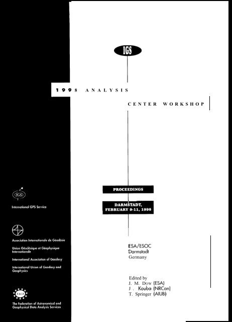
8 A N A L Y S I S 

CENTER WORKSHOP 

, 

I 

ESA/ESOC 

Darmstadt 

Germany 

Edited by 

J. M. DOW (ESA) 

J. Kouba (NRCan) 

T. Springer (AIUB)

The research described in this publication was sponsored by many agencies who actively 

participate in the International GPS Service. The Proceedings of the Workshop were prepared 

and published by the European Space Centre of the European Space Agency.

FOREWORD 

The 1998 Analysis Centre Workshop of the International GPS Service for Geodynamics (IGS) 

held in Darmstadt, Germany from 9 to 11 February 1998 followed a series of workshops 

dedicattxl to IGS Analysis Centre issues (1993 in Ottawa, 1994 in Pasadena, 1995 in Potsdam, 

1996 in Silver Spring, 1997 in Pasadena; IGS workshops with a more general scope also took 

place in Bern in 1993 and Paris in 1994). 

Discussions between representatives of the Analysis Centres present at IGS Governing Board 

meetings and Retreat held in San Francisco and Napa Valley in early December 1997 led to the 

identification of four major topics for the upcoming workshop, which were summarised as 

follows in the invitation to participate which was sent to some 70 persons from the IGS and user 

communities: 

Topic 1: The IGS Analysis Products and Consistency of the Combination Solutions 

The basic IGS analysis products (orbits, earth orientation parameters, clocks) are of very high 

quality, and should in general be more accurate and reliable than the solutions obtained by the 

individual analysis centres (ACS). This session will focus on the current combination process, 

reporting andfeedback, along with possible enhancements in precision, consistency, robustness 

and results presentation. Furthermore, it should address a need (if any) for additional (global) 

products in order to meet current and fiture needs of IGS users. 

Topic 2: Orbit Prediction and Rapid Products 

The IGS is facing ever increasing demands for more precise and more rapid (real-time!) 

products. The computation of the rapid orbits and especially the orbit predictions, which are 

available in real-time, therefore are becoming more important and deserve special attention. 

This session will focus on ways of improving the quality of the rapid and predicted orbits. The 

current AC methods of generating the rapid products will be reviewed. The main objective will 

be the improvement of the (orbit) models and the reduction of turn-around time. 

Topic 3: IGS Reference Frame Realization and Contributions to ITRF 

The stability of the underlying reference @ame defined by the global GPS network has been 

degrading due to the decrease in quality and availability of some stations of the previously 

selected group of 13 ITRF stations. More lTRF stations and a new approach to solving this 

problem is urgently required. The future IGS reference frame realisation should be precise, 

robust and based on the GNAAC station combinations (G-SINEXes). Furthermore, the IGS 

reference frame realization should ensure a high product consistency in particular for 

orbitstEOP and the slation coordinate (G-SINEX and P-SINEX) combinations. The new ITRF96 

should be discussed in this session. 

Topic 4: XGS products for Troposphere and Ionosphere 

Global tropospheric and ionospheric information can enhance precision andlor eflciency of 

various GPS and VLBI solutions (including LEO applications). Additionally it is also required 

for (global) calibration of ground and satellite based atmospheric (i.e. troposphericlionospheric) 

determination by GPS. A combined IGS solution for tropospheric zenith biases already shows 

. . . 

Ill

considerable promise. The IGS global ground network is also allowing progress to be made in 

development of regional and global ionospheric maps. Of particular interest is lhe assimilation 

of such maps into global models which may be based on atmospheric physics andlor on 

alternative sources of measurement data. The main objective will be to dejlne an operational 

IGS ionospheric product (or products). 

Fifty-one active participants representing institutions in more than a dozen different countries 

(USA, Canada, Australia, France, UK, Switzerland, Italy, Spain, Norway, Denmark, Belgium, 

The Netherlands and Germany) contributed through presentation of papers, posters and intensive 

discussion to the workshop. The Proceedings which are documented in the present volume 

contain, in addition to introductory material (including the IGS Chairman’s Report and the 

Summary Recommendations of the Workshop), a total of 25 full papers, 4 abstracts and 7 poster 

summary papers, covering in particular all workshop contributions relating to the 4 major topics. 

I would like to thank all participants for their active involvement in the workshop, and to the 

speakers and poster presenters who, by the quality of their contributions during the workshop 

itself and rapid preparation of their manuscripts afterwards, once again demonstrated the 

amazing motivation of those involved in the IGS, The “Position Papers” relating to the key 

topics mentioned above were prepared in a short time and distributed to all participants in 

advance of the workshop. The authors (T. Springer, J. Zumberge, J. Kouba; T. Martin-Mur, T. 

Springer, Y. Bar-Sever; J. Kouba, J. Ray, M. Watkins; G. Gendt; J. Feltens, S. Schaer), working 

together by e-mail, made a fundamental contribution to the preparation and to the successful 

outcome of the workshop. 

Thanks are due to the members of the Local Organizing Committee (Siegrnar Pallaschke, 

Roberta Mugellesi Dow and Hiltrud Grunewald) for smooth organisation of the workshop 

logistics, the reception and visit to the satellite control facilities at ESOC, and the workshop 

dinner at Jagschloss Kranichstein. 

The Scientific Programme Committee for the 1998 IGS Analysis Centre Workshop consisted 

of myself (as representative of the host institution), Jan Kouba (as IGS Analysis Centre 

Coordinator from 1994 to 1998) and Tim Springer (as future IGS AC Coordinator). Although 

we three also appear as editors, I would like to dedicate these proceedings to Jan Kouba with 

thanks for his massive contribution to the IGS analysis efforts since the beginning of the IGS, 

a contribution which will be difficult to match and will certainly not end with his retirement 

from Natural Resources Canada. 

John M. Dow 

ESA/ European Space Operations Centre 

Darmstadt 

April 1998 

iv

TABLE OF CONTENTS 

Foreword . . . . . . . . . . . . . . . . . . . . . . . . . . . . . . . . . . . . . . . . . . . . . . . . . . . . . . . . . . . . . . . . . . . . . . . . . . . . . . . . . . . . . . . . . . . . . . . . . . . . . . . . . . . . . . . . . . . . . . .........iii . 

J.M. DOW 

Programmeof Workshop . . . . . . . . . . . . . . . . . . . . . . . . . . . . . . . . . . . . . . . . . . . . . . . . . . . . . . . . . . . . . . . . . . . . . . . . . . . . . . . . . . . . . . . . . . . . . . . . . . . . . ..l . 

List of Ptiicipmts . . . . . . . . . . . . . . . . . . . . . . . . . . . . . . . . . . . . . . . . . . . . . . . . . . . . . . . . . . . . . . . . . . . . . . . . . . . . . . . . . . . . . . . . . . . . . . . . . . . . . . . . . . . . . . . ...7 

Executive SmV . . . . . . . . . . . . . . . . . . . . . . . . . . . . . . . . . . . . . . . . . . . . . . . . . . . . . . . . . . . . . . . . . . . . . . . . . . . . . . . . . . . . . . . . . . . . . . . . . . . . . . . . . . . . . ...9 

G. Beutler 

Summary Recommendations of the Darrnstadt Workshop . . . . . . . . . . . . . . . . . . . . . . . . . . . . . . . . . . . . . . . . . . . . . . . . . ..l9 

Recommendation and Action Items of the IGS Governing Board Retreat, 

Napa Valley, December 12-14 1997 . . . . . . . . . . . . . . . . . . . . . . . . . . . . . . . . . . . . . . . . . . . . . . . . . . . . . . . . . . . . . . . . . . . . . . . . . . . . . . . . . . ...25 

1.1. Mueller 


The IGS analysis products and the consistency of the combined solutions . . . . . . . . . . . . . . . . . . . . . . . ...37 

Z Springer, J. Zumberge, J Kouba 

Efficient estimation of precise high-rate GPS clocks . . . . . . . . . . . . . . . . . . . . . . . . . . . . . . . . . . . . . . . . . . . . . . . . . . . . . . . . . ...55 

(Abstract only) 

J. Zumberge, F. Webb, M. Watkins 

Precise high-rate satellite clocks at GFZ . . . . . . . . . . . . . . . . . . . . . . . . . . . . . . . . . . . . . . . . . . . . . . . . . . . . . . . . . . . . . . . . . . . . . . . . . . . . ...57 

W. Sohne 

The IGS/BIPM time transfer project . . . . . . . . . . . . . . . . . . . . . . . . . . . . . . . . . . . . . . . . . . . . . . . . . . . . . . . . . . . . . . . . . . . . . . . . . . . . . . . . . . ...65 

J. Ray 


Orbit predictions and rapid products . . . . . . . . . . . . . . . . . . . . . . . . . . . . . . . . . . . . . . . . . . . . . . . . . . . . . . . . . . . . . . . . . . . . . . . . . . . . . . . . . . ...73 

T. Martin-Mur, T. Springer, Y. Bar-Sever 

A new solar radiation pressure model for the GPS satellites . . . . . . . . . . . . . . . . . . . . . . . . . . . . . . . . . . . . . . . . . . . . . ...89 

T. Springer, G. Beutler, M, Rothacher 

New solar radiation pressure models for GPS satellites . . . . . . . . . . . . . . . . . . . . . . . . . . . . . . . . . . . . . . . . . . . . . . . . . . . . ..l07 


Y. Bar-Sever, D. Jefferson, L. Remans 

v

A look at the IGS predicted orbit . . . . . . . . . . . . . . . . . . . . . . . . . . . . . . . . . . . . . . . . . . . . . . . . . . . . . . . . . . . . . . . . . . . . . . . . . . . . . . . . . . . . . ..l . O9 


J. Zumberge 

Real time ephemeris and clock corrections for GPS and GLONASS Satellites . . . . . . . . . . . . . . . . . 111 

M. Romay-Merino, J Nieto-Recio, J Cosmen-Shortmann, J. Martin-Piede[obo 

Potential use of orbit predictions and rapid products in the GWS programme . . . . . . . . . . . . . . . . . 127 

P. Silveslrin 

Topic 3: IGS Reference Frame Realisation and Contributions to ITRF 

IGS reference frame realisation . . . . . . . . . . . . . . . . . . . . . . . . . . . . . . . . . . . . . . . . . . . . . . . . . . . . . . . . . . . . . . . . . . . . . . . . . . . . . . . . . . . . . . . ..l39 . . 

J, Kouba, J. Ray, M. Watkins 

1TRF96 and follow-on for 1998 . . . . . . . . . . . . . . . . . . . . . . . . . . . . . . . . . . . . . . . . . . . . . . . . . . . . . . . . . . . . . . . . . . . . . . . . . . . . . . . . . . . . . . . ..l73 . 

C. Boucher, Z. Altamimi, P. Sillard 

IGS reference stations classification based on ITRF96 residual analysis . . . . . . . . . . . . . . . . . . . . . . . . . . . 177 

Z. Ahamirni 

Estimation of nutation terms using GPS . . . . . . . . . . . . . . . . . . . . . . . . . . . . . . . . . . . . . . . . . . . . . . . . . . . . . . . . . . . . . . . . . . . . . . . . . . . ..l83 

M. Rothacher, G. Beutler 

Globally consistent rigid plate motion: Fiducial-free Euler vector estimation . . . . . . . . . . . . . . . . . . . 191 

G. Blewitt, R. Kawar, and P. Davies 

Topic 4: IGS Products for Troposhpere and Ionosphere 

IGS Combination of tropospheric estimates - experience from pilot experiment . . . . . . . . . . . . . ..2O5 

G. Gendt 

Water vapour from observations of the 

German Geodetic GPS reference network (G~F) . . . . . . . . . . . . . . . . . . . . . . . . . . . . . . . . . . . . . . . . . . . . . . . . . . . . . . . . . . ..2l7 . 

(summary) 

M. Becker, G. Weber, C. Kopken 

Estimating horizontal gradients of tropospheric path delay 

with a single GPS receiver . . . . . . . . . . . . . . . . . . . . . . . . . . . . . . . . . . . . . . . . . . . . . . . . . . . . . . . . . . . . . . . . . . . . . . . . . . . . . . . . . . . . . . . . . . . . . . . ...223 


Y. Bar-Sever, P. Kroger, J. Borjesson 

IGS products for the ionosphere . . . . . . . . . . . . . . . . . . . . . . . . . . . . . . . . . . . . . . . . . . . . . . . . . . . . . . . . . . . . . . . . . . . . . . . . . . . . . . . . . . . . . . . ...225 

J. Feltens, S. Schaer 

IONEX: The Ionosphere Map EXchange, Format Version 1 . . . . . . . . . . . . . . . . . . . . . . . . . . . . . . . . . . . . . . . . . ...233 

vi

S. Schaer, W. Gurtner, J Feltens 

The study of the TEC and its irregularities using a regional network 

of GPS stations . . . . . . . . . . . . . . . . . . . . . . . . . . . . . . . . . . . . . . . . . . . . ..- . . . . . . . . ..- . . . . . . . . ..--- . . . . . . . ...-...-......................-..-...249 

R. Warnant 

Monitoring the ionosphere over Europe and related ionospheric studies . . . . . . . . . . . . . . . . . . . . . . . . . . .265 

N. Jakowski, S. Schluter, A. Jungstand 

Routine production of ionospheric TEC maps at ESOC - first results . . . . . . . . . . . . . . . . . . . . . . . . . . . . . . .273 

J. Feitens, J. Dow, T. Martin-Mur, C. Garcia-Martinez, P. Bernedo 

Chapman profile approach for 3-D global TEC representation . . . . . . . . . . . . . . . . . . . . . . . . . . . . . . . . . . . . . . . ...285 

1 Feltens 

The role of GPS data in ionospheric monitoring, mapping and nowcasting . . . . . . . . . . . . . . . . . . . . ...299 

1?. Leitinger 

Mapping and predicting the ionosphere . . . . . . . . . . . . . . . . . . . . . . . . . . . . . . . . . . . . . . . . . . . . . . . . . . . . . . . . . . . . . . . . . . . . . . . . . . . . ..3O7 

S. Schaer, G. Be-utler, M. Rothacher 

Contributed papers on other topics 

Experiences of the BKG in processing GLONASS and combined 

GLONASS/GPS observations . . . . . . . . . . . . . . . . . . . . . . . . . . . . . . . . . . . . . . . . . . . . . . . . . . . . . . . . . . . . . . . . . . . . . . . . . . . . . . . . . . . . . . . . . . . 321 . . 

H. Habrich 

Precise autonomous ephemeris determination for fiture navigation satellites . . . . . . . . . . . . . . . . ...333 

M. Romay-Merino, P. van N@-ik 

ARP project: Absolute and relative orbits using GPS . . . . . . . . . . . . . . . . . . . . . . . . . . . . . . . . . . . . . . . . . . . . . . . . . . . . . . ...347 

T, Martin-Mur, C. Garcia-Martinez 

Poster Summary Papers 

IGS related activities at the Geodetic Survey Division 

of Natural Resources Canada . . . . . . . . . . . . . . . . . . . . . ..-. - . . . . ..- . . . . . . . . ..- . . . . . . . . . . . . . . . . . . . . . . . . . .." . . . . . .." . . . . ...-.....353 

C. Huot, P Tktreault, Y. Mireault, P. H&oux, R. Ferland, D. Hulchison and J. Kouba 

ESWESOC IGS Analysis Centre poster sum~ . . . . . . . . . . . . . . . . . . . . . . . . . . . . . . . . . . . . . . . . . . . . . . . . . . . . . . . . . . ...357 

C. Garcia-Martinez, J. Dow, T. Martin-Mur, J Feltens, P. Bernedo 

Recent IGS Analysis Center Activities at JPL . . . . . . . . . . . . . . . . . . . . . . . . . . . . . . . . . . . . . . . . . . . . . . . . . . . . . . . . . . . . . . . . . ...363 

D. Jefferson, Y. Bar-Sever, M. Hejlin, M. Watkins, F. Webb, J. Zumberge 

A review of GPS related activities at the National Geodetic Survey . . . . . . . . . . . . . . . . . . . . . . . . . . . . . . . ...367 

vii

M. Schenewerk, S. Mussman, G. Mader and E. Dutton 

U.S. Naval Observatory: Center for rapid service and predictions . . . . . . . . . . . . . . . . . . . . . . . . . . . . . . . . . . ...375 

J. Ray, J Rohde, P. Kammeyer and B. Luzum 

The IGS Regional Network Associate Analysis Center for South America at DGFI . . . . . . ...38 1 

W. Seemiiller, H. D-ewes 

The Newcastle Global Network Associate Analysis Centie . . . . . . . . . . . . . . . . . . . . . . . . . . . . . . . . . . . . . . . . . . . . ...395 

R. Kawar, G. Blewitt and P. Davies 

IGS Workshop Dinner, JagdschloJ3 Kranichstein, Darrnstadt . . . . . . . . . . . . . . . . . . . . . . . . . . . . . . . . . . . . . . . . . . . . .399 

. . . 

Vlll

Programme of Workshop 

1

I 

Qesa - >% 

~) 

,.. ..-” ‘ 

.’-..+ 

,! 

m=li::=~llllilw:= m::m 

., 

&$ :? 

. . . . 

IGS ANALYSIS CENTRE WORKSHOP 1998 

Sunday 8 February 1998 

16:00 IGS Governing Board (GB) Business Meeting (separate invitation by Central Bureau) 

Monday 9 February 

08:15 Opening of Workshop registration desk 

09:00 Welcome and introduction (J.M. Dow, C. Mazza, G. Beutler) 

09:20 1. Mueller: Summary of conclusions of the GB Retreat 

Topic 1: The lGS Analysis Products and Consistency of the Combination Solutions 

(Session chair: J. Kouba, M. Rothacher) 

09:40 Poshion paper by T. Springer, J. Zumberge, J. Kouba 

10:00 J. Zumberge: Efficient estimation of precise high-rate GPS clocks 

10:15 W. Soehne: Precise high-rate satellite clocks at GFZ 

10:30 J. Ray: The IGWBIPM time transfer project 

10:45 Coffee break 

11:00 Discussion 

12:15 Lunch 


(Session chair: T. Springer, J. Dow) 

13:30 

13:50 

14:10 

14:25 

14:40 

14:55 

15:30 

15:45 

18:00 

Position paper by T. Martin-Mur, T. Springer, Y. Bar-Sever 

T. Springer, Y. Bar-Sever: Radiation pressure models for GPS 

J. Zumberge: Identification of mismodelled satellites in the GPS predicted orbit 

M. Romay-Merino: Real-time ephemeris corrections for EGNOS based on the computation of accurate 

orbit predictions 

P. Silvestrin: The GRAS programme and projected requirements for orbit prediction and rapid products 

Discussion 

Coffee break 

Analysis Centre Poster Session 

Reception with buffet at ESOC 

3

@esa m=l, ::=mlllll lx= mj:n 

IGS ANALYSIS CENTRE 

Tuesday 10 February 

Topic 3: lGS Reference Frame Realization and Contributions to ITRF 

(Session chair: M. Watkins, G. Beutler) 

09:00 Position paper by J. Kouba, J. Ray, M. Watkins 

09:20 C. Boucher, Z. Altamimi, P. Sillard: ITRF96 and follow-on for 1998 

. ,...~ .> 

e . .. . ..7 

@esa -=ll::=~llill[*:= *::H 

IGS ANALYSIS CENTRE WORKSHOP 199S 

Wednesday 11 February 

09:00 

09:10 

09:20 

09:35 

09:50 

10:05 

10:20 

10:30 

10:50 

13:00 

14:30 

Contributed papers on other topics 

(Session chair: Peng Fang) 

Y. Bar-Sever: Low elevation tracking by TurboRogue receivers 

Y. Bar-Sever, K. Hurst: Site specific antenna phase center calibrations 

H. Habrich: Experiences of the Federal Office for Cartography and Geodesy (BKG) in processing 

GLONASS and combined GLONASS/GPS observations 

M. Romay-Merino: Precise autonomous orbit determination for future navigation satellites without 

degradation during manoeuvres 

T. Martin-Mur, C. Garcia-Martinez: ARP project - absolute and relative orbits using GPS 

R. Neilan: Status of GPS modernisation effort in the US, including prospects for additional civilian 

frequencies 

Free slot 

Coffee break 

Discussion on open AC issues (Facilitators by topic groups: J. Dow, J. Kouba, T. Springer) 

End of workshop 

Wrap-up Business Meeting ( GB/CB members, session coordinators)

,.,,. ,:, -.. ., ,,.Y 

@esa 9=II::=RIII;IJ*: =M::m @iisEJ 

,-.:. 

.+ I&s : 

,., , . 

3 . . ....+ ‘“ 

Posters 

1. 

2. 

3. 

4. 

5. 

6. 

7. 

8. 

9. 

10. 

11. 


CODE Analysis poster 

EMR Analysis poster 

ESA Analysis poster 

GFZ Analysis poster 

JPL Analysis poster 

NGS Analysis poster 

S10 Analysis poster 

USNO Analysis Poster 

Newcastle GNACC processing/ results 

GFZ CHAMP poster and S/C model 

SIRGAS (South America) RNAAC poster 

6

@esam=,,: .= B31111112’Z=EJ!:O 


Zuheir Altamimi, lnstitut Geographique National, France 

Poul Hoeg Andersen, TERMA (CRI), Denmark 

Yoaz Bar-Sever, JPL, USA 

Matthias Becker,BKG Frankfurt, Germany 

Pelayo Bemedo, ESA/GMV 

Gerhard Beutler, Univ. of Bern, Switzerland 

Geoff Blewitt, Univ. of Newcastle, UK 

Claude Boucher, lnstitut Geographique National, France 

Carine Bruyninx, Royal Observatory of Belgium 

Stefano Casotto, Univ. of Padova, Italy 

Bill Dillinger, NOAA, USA 

John Dow, ESA 

Bjom Engen, Statens Kartverk, Norway 

Peng Fang, Scripps Institution of Oceanography, USA 

Joachim Feltens, ESA/eds 

Remi Ferland, Natural Resources Canada 

Walter Flury, ESA 

Daniel Garnbis, Observatoire de Paris, France 

Carlos Garcia-Martinez, ESA/GMV 

Gerd Gendt, GFZ Potsdam, Germany 

Ramesh Govind, AUSLIG, Australia 

Heinz Habrich, BKG Frankfurt, Germany 

Caroline Huot, Natural Resources Canada 

Norbert Jakowski, DLR, Germany 

Klaus Kaniuth, DGF1, Germany 

Ra’ed Kawar, Univ. of Newcastle, UK 

Jan Koub~ Natural Resources Canada 

Reinhart Leitinger, Univ. of Graz, Austria 

Tomas Martin-Mur, ESA 

Carlo Mazza, ESA 

Ivan Mueller, Ohio State University, USA 

Rolf Muench, ESA 

Roberta Mugel lesi Dow, ESA 

Ruth Neilan, JPL,, USA 

Guillermo O-legq ISA 

List of Participants 

7 

Siegmar Pallaschke, ESA 

I Ians Peter Plag, Statens Kartverk, Norway 

Mostafa Rabah, TU Darmstadt, Germany 

Jim Ray, USNO, USA 

Jim Rhode, USNO, USA 

Miguel Romay, GMV, Spain 

Marita Roth, ESA 

Markus Rothacher, Univ. of Bern, Switzerland 

Stefan Schaer, Univ. of Bern, Switzerland 

Mark Schcnewcrk, NOAA, USA 

Wolfgang Secmueller, DGF1, Gcrrnany 

Pierluigi Silvestrin, ESA 

Wolfgang Soehne, GFZ Potsdam, Germany 

Tim Springer, Univ. of Bern, Switzerland 

Lambert Wanninger, TU Dresden, Germany 

Rene Warnant, Royal Observatory of Belgium 

Mike Watkins, JPL, USA 

Georg Weber, BKG Frankfurt, Germany, Austria 

Pascal Willis, Institut Geographique National, France 

Jim Zumberge, JPL, USA

EXECUTIVE SUMMARYl 

G. Beutler 

The 1998 IGS Analysis Center Workshop took place 9-11 February 1998 in Darrnstadt. In 

addition, a business meeting of the IGS Governing Board was scheduled for Sunday, February 

8, a wrap-up meeting of the Governing Board together with the convenors of the AC Workshop 

and the authors of the position papers concluded the Darmstadt IGS events. As usual I try to 

summarize the essential events of the Board meetings and of the workshop. 

Governing Board Meetings (February 8 and 11) 

IGEX-98 

Pascal Willis, chair of the CSTG Subcommission on “Precise Satellite Microwave Systems”, 

presented the draft call for participation for the “International GLONASS Experiment (IGEX)” 

to the IGS Governing Board. In essence it is proposed to organize a three months GLONASS 

test campaign by the end of 1998. The Experiment is organized by CSTG, it is sponsored by 

the IGS, the ION, and the IERS. The call for participation was prepared by the IGEX steering 

committee consisting of Pascal Willis (IGN, chair), Gerhard Beutler (AIUB), Werner Gurtner 

(AIUB), Guenther Hein (UFAF), Ruth Neilan (JPL), and Jim Slater (NIMA). 

The draft call for participation consists of two parts, a description of the experiment and the 

actual call for participation. The IGS involvement is indeed essential: Major parts of the IGS 

infrastructure (network, data links, data centers) will be used. It is furthermore expected that 

some of the IGS Analysis Centers will answer the IGS Call for Participation. 

The Steering Committee of the IGEX-98 is fostering participation in the 1998 International 

GLONASS Experiment IGEX-98 in the following areas: 

- IGEX-98 Coordinating Center 

- IGEX-98 Observing Sites 

- IGEX-98 Data Centers 

- IGEX-98 Analysis Centers 

- IGEX-98 Evaluation Center(s) 

All GLONASS satellites are equipped with arrays of LASER reflectors allowing the SLR 

community to range easily (!) to the GLONASS satellites. It was thus decided to closely 

coordinate the IGEX-98 with the SLR 

SubCommission of CSTG (Werner Gurtner from the IGEX-98 steering committee is the “liaison 

officer” to the SLR Subcommission). The participation of the SLR community is essential for 

validating the results and for the development of radiation pressure models for the GLONASS 

satellites. 

The receiver situation is of concern to the IGS Board members. In principle one would like to 

use uniquely geodetic-type dual fi-equency combined GPS/GLONASS equipment (similarly as 

it was done for the 1992 IGS Test Campaign). In order to have access to a greater number of 

‘Reprint of IGS Mail No. 1806, 17 February 1998. 

9

eceivers the steering committee decided to be more flexible: In sequence of preference, the 

following receiver types may be used in IGEX-98: 

● Combined dual-frequency GPS/GLONASS receivers 

● Dual-frequency GLONASS receivers 

● Combined single-frequency (Ll) GPS/GLONASS receivers 

● Single-frequency GLONASS receivers 

Receivers must be collocated with or tied to sites that have well-determined ITRF coordinates. 

IGS sites are preferable. The ITRF coordinates should have an accuracy of 1-5 cm. 

Not only the receiver situation, but also the satellite situation has to be considered as a crucial 

issue. Today, there are only 14 operational GLONASS satellites available, Launches of 

GLONASS satellites have been announced, however. There is not much that the steering 

committee can do to improve satellite availability (!). Should the number of operational 

GLONASS satellites fall under a critical level, the IGEX-98 would of course have to be 

postponed. 

The schedule for IGEX-98 is as follows: 

February 1998 Distribution of IGEX-98 Call for Participation 

May 

June 

September 20 

December 20 

early 1999 

through mail e-mail services of the sponsoring 

agencies. 

Proposals due 

Evaluation of proposal by the Steering Committee 

Review/approval of the schedule 

Designation of the Oversight Committee (including Chair) 

Campaign Planning Meeting 

Campaign begins 

Campaign ends 

IGEX-98 Evaluation Workshop (possibly combined with the 1999 IGS 

Analysis Center Workshop) 

The IGS Governing Board discussed the proposal in detail. It was finally decided that the Call 

for Participation should be sent out in February 1998 after a few modifications. The 

modifications underline the experimental (as opposed to operation oriented) character of 

IGEX-98. The chairman thanked Pascal Willis and the IGEX-98 steering committee for their 

planning work. 

IGS Densification 

At the eighth IGS Governing Board meeting in San Francisco (December 1998) it was decided 

to take the necessary steps to terminate the Pilot Phase of the Densification Project as soon as 

possible, but not before all discrepancies, errors, etc., in the understanding of station coordinates 

(and velocities) were removed (IGS Mail Message 1763). This condition could not yet be met. 

The IGS Central Bureau, together with the IGS Infrastructure Committee are still working on 

that issue. The basis is the list of discrepancies published regularly by the Analysis Coordinator. 

It is the policy of the IGS Governing Board to come up with a unique IGS product of 

coordinates and station velocities. As all three GNAACS are willing to continue with their 

10

activities one has the problem that a unique series of coordinates has to be formed using the 

resulting SINEX fdes of the three SINEX files. Nom-m Beck, Chief of Active Control System, 

Natural Resources Canada (NRCan), kindly offeral in a letter dated January 19, 1998 to produce 

the SINEX GNAAC combination, based on the three GNAAC solutions by University of 

Newcastle, JPL and MIT, The IGS Governing Board unanimously accepted this offer and asked 

the chaimmn to thank NRCan for providing this service to the IGS community. NRCan will start 

providing this combination as soon as possible (probably in March 1998). 

As a side issue Norman Beck asked the chairman to explore the IGS Governing Boards views 

concerning an EUREF-like activity for North America. The discussion revealed that the Board 

and the GNAACS represented at the business meeting would in fact favour such a development. 

The EUREF solution, coordinated by Carine Bruyninx, is (amongst other) most useful to 

eliminate all station-related problems. Also, it makes sure that the solution is actually providing 

the reference frame for the continent, which is accepted and used by the European topography 

and geodetic services, The chairman was asked to write a letter to the existing and potential 

RNAACS in North America encouraging this level of cooperation. 

“Densification of the ITRF using GPS” will be again on the agenda of the 

ninth IGS Governing Board Meeting, to be held end of May 1998 in Boston. I 

hope (and assume) that the Board will be in a position to decide about the 

operational phase of the densification issue. 

1997 IGS Annual Report 

Ruth Neilan and Jim Zumberge came up with a new format for the 1997 IGS Annual Report. 

They propose to produce the report in two parts (corresponding to 2 volumes). Part 1 would 

contain, so to speak, the top level information (CB report, IGS Analysis Center Coordinator 

report, report about current projects, etc.), Part 2 would contain the Analysis Center reports, the 

station reports, etc. Part 1 would be edited by the Central Bureau in a similar way as it was done 

with the 1996 Annual Report. Part 2 would be published based on “camera ready manuscripts”. 

In order to reduce the size of the Annual Repoti, page limits will be given to the authors. Both 

reports will be made available also in electronic form. 

The proposal aims at reducing the costs of the Annual Reports and at having the Annual Report 

available much earlier. 

After extensive discussions and after positive feedback from the Analysis Centers the Board 

accepted the proposal. The authors of the 1997 Annual Report will be notified concerning the 

expected contributions in the near future. The Annual report -- if possible both parts, but 

certainly Part 1 should be available in July 1998. 

GPS Modernization Process and IGS Involvement 

Ruth Neilan informed the Board that she was asked to chair a working group of the “US GPS 

Interagency Advisory Council (GIAC)” jointly setup by the U.S. Department of Defence (DoD) 

and the Department of Transportation (DoT). Ruth Neikm views this assignment as an important 

interface between the international scientific community represented in the IGS and operators 

of the GPS. 

The IGS Governing Board in turn viewed this as a very positive development and encouraged 

11

the Central Bureau to play a very active role in this working group. The hope was expressed that 

views of the IGS community on issues like the “second civil frequency” or on the attempt to 

assign the frequency range 1559-1567 MHz to Mobile Satellite Services (MSS) (latest attempt 

made at the the WRC-97 in Geneva) could more easily be made known. The CB was in 

particular asked to coordinate efforts in such matters with other organizations like, e.g., the ION. 

IGS Retreat, December 1998 

At the seventh IGS Governing Board Meeting in Rio de Janeiro it was decided to organize an 

“IGS Retreat” in December 1997 with the IGS Governing Board Members and a very limited 

group of IGS Associates with the goal to come up with a plan for the future development of the 

IGS which then should be discussed by the entire IGS community and the Board (IGS Mail 

Message No 16S3). 

About half of the time of the Sunday business meeting of the IGS Governing Board was devoted 

to the discussion of the “recommendations and action items” of the IGS Governing Board retreat 

in Napa Valley, December 12-14, 1997. The report was prepared by Ivan I. Mueller, who was 

also the program chair of the retreat. It was clear that the report could only be discussed 

at the business meeting; decisions on this matter will be taken at the next official IGS Governing 

Board Meeting (28 May 1998 in Boston). The complete report containing all recommendations 

and action items may be retrieved by ftp (see attachment). Let me point out that comments on 

the action items and recommendations are welcome!: no decisions have been taken so far, the 

process may still be influenced till the end of May. 

The report contains fourteen recommendations and thirteen action items emerging from them. 

Let me comment a few of these recommendations and action items. 

Recommendation 1 proposes to change the name “International GPS Service for Geodynamics” 

to “International GPS Service”. The acronym “IGS” remains the same. The Board is in favour 

of this recommendation. 

Remmrnendation 2 asks the “IGS to produce combined, internally consistent, global products”. 

Product will include in future orbit parameters, station coordinates and velocities, earth rotation 

parameters, GPS clock corrections, IGS time scale, tropospheric zenith delays, and ionosphere 

models. Consistency of all products is the central issue, which was also discussed at the 

workshop (see below). The IGS/BIPM Project addresses the time-related issues. 

Recommendation 5 asks that “the global IGS Network should be enhanced in the overall sense”. 

An important (actually THE important) action item related to this recommendation is to appoint 

a Network Manager or Coordinator, within or outside the CB. 

Recommendation 7 asks for a review of the definition of the terms “IGS Analysis Center”, 

“Associate Analysis Center” at the Analysis Center Workshop in Darrnstadt. 

Recommendation 8 recommends that Working Groups be appointed for “troposphere products”, 

“ionosphere products”, for “ITRF densification”, and possibly for others. The working groups 

should have clear charters and structures. 

Recommendations 9 to 12 are related to the IGS Central Bureau. It is in particular recommended 

that the tasks of the CB (as described in the Terms of Reference) are regularly reviewed, that 

12

future tasks are clearly defined. Moreover, requirements concerning the minimum number of 

persons working for the CB were stated. 

Recommendation 14 asks the Governing Board to consider forming a committee, with external 

participation, with the task to prepare the IGS Long Range and Strategic Plan. 

The above selection of recommendations and action items emerging from the IGS Retreat 1997 

is of course a personal one. Everybody is encouraged to retrieve the complete report. 

The Governing Board considers the “recommendations and action items” of the IGS Governing 

Board retreat in Napa Valley, December 12-14, 1997 as prepared by Ivan I. Mueller as an 

extremely useful document defining the development of the IGS at least till the end of the 

millenium (!). The Board thanked Ivan I. Mueller for his excellent work. 

1998 IGS Analysis Center Workshop (9-11 February, 1998) 

4 topics (see below) were dealt with in detail at the 1998 IGS Analysis Center Workshop. The 

first presentation within each topic was a position paper, topic 4 even was dealt with in two 

position papers. AU of the position papers were available over the internet prior to the workshop 

(ftp-address: see attachment). The final versions of the position papers will be available no later 

than March 15, 1998 under the same ftp-address. These remarks underline how well the 

workshop was prepared by the prograrnme committee, consisting of John Dow, Jan Kouba, and 

Tim Springer. 

The workshop was formally opened on Monday, February 9 at 9 a.m. with a welcome address 

by Carlo Mazza, Head of Ground Systems Engineering Department of ESA, with an introduction 

by John Dow, and an overview of previous IGS workshops by Gerhard Beutler. 


(Session Chair: Jan Kouba, Markus Rothacher) 

The position paper entitled “the IGS Analysis Products and the Consistency of the Combined 

Solutions” written by T.A. Springer, J.F. Zumberge, and J. Kouba reviewed the quality, 

consistency, and reliability of current IGS analysis products (orbits, Earth orientation 

parameters, station coordinates, and clocks). The paper focused on current procedures to derive 

these products, on reporting and feedback. Seven recommendations were given at the end of the 

paper. All of them were accepted, some will ask for significant work by the IGS Analysis 

Centers in the near future, As the proceedings of the workshop (containing all position papers 

and resolutions) should be available rather soon, and as people interested in the resolutions may 

retrieve preliminary versions of the position papers under the ftp address mentioned, we may 

confine ourselves to highlight only a few of these resolutions. 

First of all it is recommended that the IGS ACS include ephemerides for ALL operational 

satellites in the daily SP3-fdes, and that these ephemerides are characterized by MEANINGFUL 

accuracy codes. No format changes are necessary for this step, most of the analysis centers 

already provide such accuracy information. It was also discussed, however, that the user 

community of IGS products must be made aware of these accuracy codes, and that this 

community should be strongly encouraged to make use of these codes. This aspect might be 

more important in future, when more orbit information of “modest quality” will available (due 

13

to this resolution). 

Precise single point positioning developed by Zumberge et al. is used extensively today. 

Consistency of orbit and clink information is crucial for this technique, The required consistency 

level (of millimeters) is much easier to achieve if the same software package is used to produce 

the global products (orbits and clocks) AND the coordinates using the single point positioning 

technique. It was/is most encouraging to see that already today, thanks to an essential upgrading 

of the combination technique, the consistency level for the combined IGS products is not far 

away from the best possible consistency level that may be reached (using one and the same 

software). It seems feasible that sub-centimeter point-positioning using IGS products should be 

possible in the very near future. 

Other recommendations dealt with the “densification project”. It was recommended that 

deadlines in compliance with other deadlines in the IGS are used, that EOP information is 

included by all analysis centers in the GNAAC solutions, and that all discrepancies/errors in the 

RINEX files are removed. 

Also, the minimal requirements (perfomnance-wise) to become an IGS Analysis Center were 

reviewed (and probably clearly defined for the first time). As this recommendation was 

extensively discussed and modified at the workshop, it is advisable to wait for the final version 

of this position paper. 

There were other interesting contributions in the first session. Jim Zumberge presented a 

technique at JPL to produce in an efficient way high-rate GPS clocks, Wolfgang Soehne from 

GFZ presented the GFZ procedures developed for the same purpose. Jim Ray gave a short status 

report of the IGS/BIPM project: the call for participation was issued in January, the next phase 

will consist of evaluating the proposals received in spring 1998. 

Topic 2: Orbit Prediction and Rapid Products (Session Chair: Tim Springer, John Dow) 

Tomas Martin Mur (ESA), Tim Springer (CODE) and Yoaz Bar Sever (JPL) reviewed the 

procedures for “Orbit Prediction and Rapid Products” in the position paper for topic 2. With the 

increasing demand for close to real-time products this issue becomes more and more important. 

It came out very clearly that data availability is THE critical issue. Global coverage is far more 

important than the number of stations (provided a minimum number of about 30 stations is 

available). 

The paper also reviewed the prediction techniques used by individual IGS Analysis Centers and 

in the combination. Usually, IGS predictions are much better than broadcast orbits (the former, 

when compared to the IGS final orbits are of about 30-50 accuracy (extrapolation over 2 days), 

the latter are of 2-3 meter accuracy). There are exceptions, however, which are not always 

predictable. Two measures may improve the reliability of IGS predicted orbits: (a) reduction 

of the delay of data availability (see primary recommendation below), (b) reduction of the 

number of “unknown” parameters for prediction process. 

New orbit models developed by Yoaz Bar-Sever at JPL and by Tim Springer at CODE axe 

promising in area (b). Only improved data transmission may help in area (a): Therefore, the frost 

arid probably the primary recommendation of the position paper asks the operational and global 

data centers to give highest priority to the delivery of stations outside Europe and North America 

(!). This does not mean, of course, that data from Europe and North America are not important; 

14 

I

ut due to the usually excellent infrastructure ftp retrieval guarantees quick availability of a 

sufficiently high number of stations (data outside these areas often have to be retrieved by the 

operational centers by telephone or other links). 

All in all seven recommendations were given in the position paper for Topic 2. The first three 

addressed data availability (including more frequent than daily data download), the third 

recommends extensive tests of the two new radiation pressure models (which are made available 

by CODE and JPL) by all IGS ACS. The other three resolutions dealt with EOP series to be used 

with the predictions, studies to improve the accuracy codes for prediction, and the use of the 

NANU messages to reduce the number of blunders. An important issue, the change of the 

deadline for the IGS Analysis Centers to deliver the rapid orbits/cops to 4 p.m. U.T. by January 

1, 1999 (from 9 p.m. U.T.), was extensively discussed at the workshop. A recommendation 

related to that topic will be contained in the final version of position paper 2. 

The position paper was followed by technical papers related to topic 2: Tim Springer presented 

his “latest and greatest” radiation pressure model and compared it to the model developed by 

Bar-Sever. Jim Zumberge addressed the problem of identifying mismodeled satellites in GPS 

predicted orbits. A presentation by M. Romay-Merino dealt with considerations concerning 

real-time orbit computation for navigation using orbit predictions of the GPS, GLONASS, etc., 

in the context of GNSS. A contribution by P. Silvestrin described the GRAS (GPS/GLONASS) 

receiver being developed by ESA for support of atmospheric sounding and other applications. 

Topic 3: IGS Reference Frame Realization and Contribution to ITRF (Session Chair: Mike 

Watkins, Gerhard Beutler) 

The position paper by J, Kouba, J. Ray and M.M. Watkins addressed “IGS Reference Frame 

Realization” within/by the IGS. It was stated in particular that the current set of 13 ITRF94 

stations and the current IGS approach to realize the ITRF are no longer appropriate. A new set 

of about ftity reference frame stations (based essentially on an IGS history of station coordinates 

AND the new ITRF96 as made available through the IERS) are about to replace the “old” set of 

13 stations. It is expected that this measure will “dramatically” improve the IGS rapid EOPS. 

This in turn will improve the Bulletin A values of the IERS. 

The paper also compares in detail the ITRF96 station positions and velocities with the purely 

IGS derived quantities for the selected fifty stations (and subsets of it). The agreement is 

excellent, indeed. It is therefore natural that recommendation 1 demands the IGS to adopt 

ITRF96 as early as March 1, 1998. 

Other recornmendations deal with technical aspects of producing the SINEX solutions, like, e.g., 

the inclusion of EOPS. Last but not least, it is recommended that a “super’’combination of 

G-SINEXes for station coordinates, velocities and EOPS is researched and initiated on behalf of 

the IGS. The participants of the workshop were very much pleased to learn that NRCan would 

take on this new combination task (compare report about GB Meeting, topic “densification”). 

Very interesting and informative presentations concerning the establishment of ITRF96 followed 

the position paper. It became quite clear that the IGS is an important contributor to the ITRF. 

The histograms dealing with coordinate awuracies are interesting, as well. It might be 

worthwhile to look into the technique speciilc aspects: it seems in particular that the distribution 

of SLR-derived height errors supports the conclusion that, due to the unproblematic modeling 

of the troposphere in SLR, the SLR determined heights may signifkantly contribute to the height 

15

datum of the ITRF96. 

Markus Rothacher et al. summarized their attempts to extract short-period nutation terms from 

CODE/IGS eop series. Apparently, for periods up to about 20 days, the results obtained by GPS 

are of equal or better quality than those obtained by VLBI. The work was motivated by the 

simple idea that “there is no reason NOT to solve for nutation drifts, if one is solving for 

led-values” ! It is expected that the results can be significantly improved, if a more appropriate 

orbit model (radiation pressure model) is adopted. 

Geoff Blewitt et al. proposed to extract “fiducial-free Euler vectors” from the GNAAC 

Polyhedron time series. The method presented allows it very well to separate “normal” plate 

motion (represented through the Euler vectors, resp. their first derivatives) from “abnormal” 

(e.g., subsidence) or “apparent” (e.g., induced through antenna changes . ..) motion. It might be 

worthwhile to explore the interest within the IGS and the IERS community for such vectors as 

a regular IGS product. 

Topic 4: IGS Products for Troposphere and Ionosphere (Session Chair: Gerd 

Gendt, Mark Schenewerk) 

Troposphere 

The position paper “IGS Combination of Tropospheric Estimates - Experiences from Pilot 

Project” was presented by Gerd Gendt from the GFZ Analysis Center, GFZ was gaining 

experience since more than one year of comparing and combining troposphere estimates for 

about 100 sites of the IGS Global Network stemming from individual IGS Analysis Centers. 

Despite the fact that rather different processing options were used by the Analysis Centers 

(different levels of differencing, different binning, different cut-off angles) the consistency level 

reached is in general quite good. There was general agreement that the combined series of total 

zenith path delays for the entire IGS network are of interest for climatological studies. Gerd 

Gendt recommends furthermore that the troposphere combination product should become an 

ofllcial IGS product, that the weekly summary reports are made publicly available (in the IGS 

report series), and that the product distribution is performed using the ftp server of GFZ. 

The IGS troposphere product would be of much greater value, if a significant number of 

permanent, accurate, reliable surface meteorology measurements series would be available. This 

is a station specific issue to be addressed by the Central Bureau, the Infrastructure Committee 

and the future Network Coordinator. 

Gerd Gendt’s recommendations were unanimously accepted, We are thus looking forward to see 

the announcement through IGS-mail that official IGS troposphere products are available. 

Matthias Becker and Georg Weber from BKG Frankfurt (former IfAG) presented a study to use 

the German permanent GPS network (GREF) to extract regional troposphere information on a 

routine basis. The results are promising and should be seen as an attempt to make optimum use 

of a permanent network. 

Yoaz Bar-Sever discussed troposphere gradient estimates performed at the JPL Analysis Center. 

He concludes that gradient estimates are significant and tend to improve station coordinate 

repeatability. The drawback has to be seen in the considerably increased number of parameters. 

Comparisons of monthly mean values for the JPL gradient parameters with those of the CODE 

Analysis Center show a good agreement. More work has to be done in this area. 

16

Ionosphere 

The position paper “IGS Products for the Ionosphere” was given by Joachirn Feltens (ESA) and 

Stefan Schaer (CODE). They reviewed the ionosphere related activities within the IGS in 

previous years and they came up with a list of ten potential participating institutions in a future 

“IGS ionosphere service”. Based on an e-mail inquiry they furthermore gave an overview of 

analysis methods and models used by the institutions mentioned. An important part of the 

presentation dealt with the definition of a future IGS ionosphere product. They recommend that 

all IGS ionosphere products 

- must be based on the IONEX format, 

b should refer to a two-dimensional grid in a (single layer) shell, 

● should refer to the same shell height, 

b should use identical reference epochs for subsequent ionosphere models, 

● that one, maybe two, time resolutions have to be agreed on, and 

● that naming conventions for ionosphere model files have to be defined. 

The authors and the interested institutions are convinced that the development of an IGS 

ionosphere product makes sense and that a continuous series of IGS products should be produced 

at least over one full 11 years cycle of solar activity. It is of particular importance that the IGS 

models are covering the next period of maximum of solar activity (years 2001-2003). The key 

recommendation was to establish a pilot phase for such an IGS ionosphere service as soon as 

possible. 

It was most encouraging that the experts in the field of ionosphere physics, in particular Drs. N. 

Jakowski (DLR Neustrelitz), R. Leitinger (TU Graz), and R. Warnant (Royal Observatory of 

Belgium, Brussels), and L. Wanninger (TU Dresden) were attending the workshop to give their 

input for the development of an IGS product. Their presentations showed that many activities 

in the ionosphere community are regional in nature -- and that there are good reasons for this. 

It became clear that the IGS (at least in a first phase) should stay out of regional ionosphere 

modeling, but should rather focus on global aspects. One had to conclude from the discussions 

that there is a great interest of the ionosphere community in a continuous series of global IGS 

ionosphere models. 

That the modeling capabilities were signifkantly improved over the last few years emerged from 

two technical presentations given by Stefan Schaer and by Joachim Feltens. The former 

presentation showed (among other) that the parameters of the CODE models maybe successfully 

predicted, the latter presentation was also addressing mathematical aspects using a so-called 

“Chapman profile approach”. 

In the discussion portion of the session and in the wrap-up meeting at the end of the workshop 

the following procedure was proposed: 

● Joachim Feltens and Stefan Schaer, in close cooperation with the existing “IGS 

ionosphere club”, should come up with 

● a proposal for global IGS ionosphere products (including the specification of parameters, 

formats, etc.) 

● a clear proposal how to proceed (test phase, pilot phase, etc.) 

● a proposal for the structure of the working group (what positions have to be created (e.g., 

IGS (Associate) Ionosphere Analysis Centers, Ionosphere Combination Center, 

Validation Center), 

b a list of members for the future IGS Ionosphere Working Group. 

17

● These specifications should be included in the final version of their position paper. 

● John Dow and Gerhard Beutler should 

- draft a general “charter” for setting up Working Groups within the IGS and 

circulate this draft within the Governing Board, 

- develop in close cooperation with the “ionosphere club” the charter for the 

ionosphere working group and circulate this draft within the “ionosphere group” 

(which probably is the nucleus for the working group). 

● Assuming that the structure of the ionosphere working group is acceptable to all parties 

interested in IGS ionosphere monitoring, the ionosphere working group should be 

established by the IGS Governing Board by the end of May 1998 in Boston. 

This procedure was unanimously accepted by the IGS Governing Board and the session 

convenors at the wrap-up meeting on Wednesday, February 11. It should thus be possible to start 

an IGS pilot ionosphere service in the near future. 

The workshop was concluded with a session addressing topics other than those treated in the 

previous four sessions. Let us mention in particular presentations by T. Martin-Mur and C. 

Garcia-Martinez (absolute and relative orbit determination using spaceborne GPS receiver), Y. 

Bar-Sever (low elevation tracking of TurboRogue receivers, site specific antenna phase center 

calibrations), H. Habrich (processing of GLONASS and combined GLONASS/GPS 

observations), and by Ruth Neilan (GPS modernization effort in the US). 

Hospitality experienced in Darmstadt 

As one may conclude from the above report, the Darmstadt IGS event really was a WORKshop. 

That the IGS Analysis Centers forma very dynamic group of enthusiasts became also clear at 

the reception on Monday evening and at the dinner at Jagdschloss Kranichstein. Despite its name 

there was no hunting before the dinner, one even had the option of a vegetarian menue (and this 

in a Jagdschloss -- “o tempera, o mores”!). 

The Analysis Centers took the opportunity to thank Jan Kouba for his personal engagement and 

his great performance as IGS Analysis Coordinator. A Swiss railway clock presented to him will 

undoubtedly help him to understand the subtleties of the IGS/BIPM project. The clock is also 

complicated enough (it has at least two buttons and may be used in at least two different ways, 

e.g., as a pocket clock or as a clock on his desk) to represent a challenge for his technical skills. 

Jan will continue to serve as IGS Analysis Center Coordinator till the end of 1998. As the next 

IGS AC Workshop will take place only in 1999, the Darmstadt workshop was presumably the 

last workshop with Jan Kouba “in command” as AC coordinator. 

The chairman also took the opportunity at the dinner to express the gratitude of all workshop 

participants to the local organizers from ESA, in particular John Dow, his wife Roberta, Siegmar 

Pallaschke, Rolf Muench, and Hiltrud Grunewald for their perfect organization of the 1998 IGS 

events in Darmstadt, 

Gerhard Beutler 

Chair, IGS Governing Board 

18

SUMMARY RECOMMENDATIONS OF THE DARMSTADT 

WORKSHOP 

Position Paper 1: The IGS Analysis Products and Consistency of the Combination 

Solutions 

1. Inclusion of all satellites, which were used in the data analysis, with meaningful accuracy 

codes in the orbit products from all individual ACS. Use of these accuracy codes, or accuracy 

measures from the long-arc analysis, to identify and consequently downweight “bad” satellites 

in the orbit combination. In addition the IGS should increase the user awareness of the 

availability and importance of the accuracy codes in the SP3 files (see also Recommendation 

4). 

2. Enhancement of clock products. All ACS which submit clocks must also submit clock 

estimates from a, yet to be determined, subset of “core time stations”! All ACS are urged to 

submit clock estimates. Furthermore the ACS are encouraged to increase the sampling rate of the 

satellite clock products to 30 seconds. A format for station and satellite clocks, also suited for 

30 seconds satellite clocks, will have to be defined. 

3. Improved and automatic feedback to Data Centers (DC) and station managers in case there 

are discrepancies between RINEX fdes and station logs, data problems and unexpected problems 

(jumps) in the station coordinate solutions. 

4. Create a central place (WVW) for feedback and information about the IGS products and their 

use. 

5. Deftition of minimal requirements for becoming an IGS AC. Any AC must produce all core 

products, i.e. orbits, EOPS, and SINEX, both on time and with sufficient (high) quality. The 

IGS terms of reference will be changed accordingly, 

6. Additional accuracy digit for the IERS/IGS EOP fde format. New format to be defined before 

June 28, 1998 by Jan Kouba in cooperation with Dennis McCarthy. 

Position Paper 2: Orbit Prediction and Rapid Products 

1, Ask the Operational, Regional and Global Data Centers to give the highest priority to the 

prompt retrieval and distribution of data from sites outside Europe and North America. 

2. Ask the Operational, Regional and Global Data Centers to investigate and implement ways 

of reducing data retrieval and distribution delays. 

3. Ask the Operational, Regional and Global Data Centers to study and implement more 

frequent down-loading of the data. 

4. Ask those Analysis Centers that are evaluating more precise radiation pressure models to 

make them publicly available, and encourage all Analysis Centers to implement and use them 

when they have been validated. 

19

5. Ask the IERS Rapid Service and the Analysis Centers to investigate and propose ways to 

obtain predicted cops (pole and UT1) for use in the calculation of IGS predicted orbits. 

6. Ask the Analysis Centers and the AC Coordinator to study, monitor, and, if possible, improve 

the fitness of the accuracy codes for the predicted orbits. 

7. Ask the A_mlysis Centers to investigate the ways and the consequences of reducing the 

turn-around time for rapid and predicted products. 

8. Review data and rapid product delivery times at July 1 and October 1 in order to evaluate the 

change of the deadline for rapid products to no later than 16:00 UTC by January 31999. 

Position Paper 3: IGS Reference Frame realisation and Contributions to ITRF 

In order to increase the IGS product consistency and to prepare ground for adaptation of the new 

approach of ITRF realizations, the following recommendations were accepted by the workshop 

participants: 

1. That IGS adopts ITRF96 as early as March 1, 1998 to replace the currently ailing and 

problematic IGS realization of ITRF94, which currently is based only on less than 13 ITRF 

stations. 

2. As an interim measure and to facilitate an immediate ITRF realization improvement it is 

recommended that the selection of the new ITRF96 station positions and velocities for a large 

subset of the RF station is finalized at this workshop. This newly selected ITRF96 set of the 47 

globally distributed IGS stations is to be used for ITRF96 realization in all IGS products 

beginning as early as March 1, 1998. IGS realization of ITRF is then accomplished by the above 

ITRF96 station coordinates/velocities together with the current official igs.snx, which contains 

antenna offset and height information in the SINEX format. 

3. That all weekly submitted AC SINEX solutions (A-SINEXes) contain the EOP of the current 

week and that the submitted AC orbits/clocks (sp3) and EOP (erp) files are consistent with the 

above A-SINEX solutions. This is essential not only for the increased IGS product consistency 

but also for the future (improved) ITRF realization and IGS products. It is recommended that 

this is implemented and ensured by all ACS by June 28, 1998. 

4. That the GN&4C combinations retain (and adjust) the submitted AC EOP information of the 

current week in their G- SINEX combined products, along with the usual station position 

solutions. It is recommended to be implemented by June 28, 1998. 

5. The SINEX extensions as outlined in the Appendix IV, allowing the minimum datum and 

transformation parameter constraints to be coded in the SINEX format, are accepted and used 

by IGS on or before March 1, 1998. Furthermore, that IGS submits the SINEX extension for 

acceptance to Prof. Tom Herring of CSTG, who is currently responsible for the SINEX format. 

This will provide a means and encouragement to ACS and other IGS users to use (minimum) 

datum constraints, as well as it allow an efficient and safe monitoring of geocenter and scale 

changes (e.g. Ray, 1997). It is further recommended that only the AC Final products, which are 

based on minimum or no datum constraints, be accepted for the IGS Final 

orbit/clock/EOP/station combinations after June 28, 1998. 

20

6. That a (super) combination of G-SINEXes for station coordinates and EOP is researched and 

initiated on behalf of IGS. This EOP (G-SINEX combination) cumulative solution would replace 

the current IGS EOP combination and it would lead to an official SINEX station solution 

product (both for global as well as the polyhedron stations). The polyhedron SINEX solutions 

could be produced by back substitution when P-SINEXes are made available to produce the IGS 

P-SINEX products (station positions/velocities only). The implementation goal should also be 

by June 28, with the official IGS SINEX (G and P) products on or before January 3, 1999 ! 

Position Paper 4a: IGS Products for the Troposphere 

1. The pilot phase for the IGS Combined Tropospheric Estimates will be finished and the 

combined zenith path delay (ZPD) estimates will become an official product. The conversion 

into precipitable water vapor will be postponed until a sufficient number of surface met packages 

is available. At the moment it is to the customer to convert the ZPD by relying both on the 

existing RINEX met files as well as on interpolation within global or regional meteorological 

fields. The product will be archived at the global Data Centers. 

2. All network operators will be encouraged to enforce the installation of met packages. 

3. The Analysis Centers should strive to constrain the RF stations during the computation of the 

tropospheric estimates to reduce the biases in the ZPD estimates as much as possible. 

4. All Analysis Centers provide TRO-SINEX files which are compatible to the weekly SINEX 

fde, i.e. the daily station coordinates of the TRO-SINEX files should refer to the site description 

blocks given in the weekly SINEX file. 

5. IGS will strive to get water vapor estimates from collocated water vapor radiometer and 

VLBL During a calibration campaign all Analysis Centers will be asked to include those sites 

in their analysis for investigation of the biases in the ZPD estimates. 

6. For each SINEX fde the shortened version *.SSC without all matrices should be archieved too. 

The ssc-fdes should be formed at the Data Centers unless the ACS already submit both *.snx and 

*.SSC. This way also * .SSC versions for all the old SINEX files can be formed. 

Paper 4b: IGS Products for the Ionosphere 

1, Initially, the IGS should focus on two kinds of products: 

(a) TEC maps in grid form and 

(b) differential code biases (DCBS). 

2. IGS TEC maps are global maps. Only global maps will be compared and perhaps combined, 

This policy may be reviewed after one year of pilot operations. 

3. All TEC maps must be delivered to the IGS in the IONEX format [Schaer et al., 1998]. TEC 

maps delivered to the IGS thus are “snapshots” of the electron density referring to a 

particular epoch and to an earth-fixed reference frame. 

4. Global TEC maps from each contributing Analysis Center are given the name cccGdddO.yyI, 

21

where ccc is a 3-figure acronym for the AC (in uppercase), “G” says that this file contains 

global maps, ddd is the day of the year, “O” indicates a daily file, yy specifies the 

2-digit year, and the last letter “I” stands for “ionosphere maps”. Example: CODGO41O.98I 

(or CODGO41O.98I.Z). These files are {compressed} and sent to the IGS Global Data Centers 

and are available to the interested user. Access Fortran routines are also made available. 

5. The daily IONEX file, as produced by an IGS Analysis Center, should have a 2-hour 

resolution referring to the epochs 01, 03, . . . . 23 hours UT. RMS files corresponding to the 

2-hourly TEC maps maybe included in the IONEX files. TEC/RMS maps refer to a 

two-dimensional grid in a single layer, The height of the single layer should be 450 km 

adopting a base radius of 6371 km. The latitude ranges from 87.5 to -87.5 degrees in steps 

of-2.5 degrees; the longitude ranges from -180 to 180 degrees in steps of 5 degrees. 

TEC/RMS values have to be given in units of 0.1 TECU. 

6. Daily sets of differential code biases (DCBS) for the GPS satellites are recommended to 

be included in IONEX fdes. The exchange of satellite-specific DCBS is IONBX-supported, too. 

Note that the DCB reference maybe chosen arbitrarily and can be taken into account in the 

combination procedure. 

22

Annex 

IGS Fiducials for ITRF Reference Frame Control, ITRF96 

47 stations, Darrnstadt AC workshop, Topic 3, Rec. #2 

id City Location lon (E) lat (N) ht (m) Agency 

algo 

areq 

braz 

brmu 

davl’ 

drao 

fair 

fort 

gode 

go12 

graz 

guam 

hark 

hob2 

i rkt 

kerg 

kit3 

kokb 

kosg 

kour 

kwjl 

lhas 

macl 

mad2 

mali 

masl 

mate 

mdo 1 

nlib 

nyal 

ohig 

onsa 

pert 

piel 

pot s 

sant 

shao 

thul 

tid2 

t rom 

tskb 

vill 

wes2 

wtzr 

yarl 

yell 

zwen 

Algonquin Park, Ontario Canada -78.0714 45.9558 201.9000 NRCan/GSD 

Arequipa 

Peru -71.4928 -16.4655 2489.9506 NASA/JPL 

Brasilia 

Brazil 

-47.8779 -15.9475 1107.0570 IBGE–JPL 

Bermuda 

Bermuda Islands -64.6963 32.3704 –10.6158 NOAA 

Davis 

Antarctica 

77.9726 -68.5773 45.4584 AUSLIG 

Penticton 

Canada 

-119.6250 49.3226 542.8755 NRCan/GSC 

Fairbanks, AK 

USA 

-147.4990 64.9780 320.0126 JPL–GSFC 

Fortaleza 

Brazil 

–38.4256 -3.8774 20.4850 NOAA 

Greenbelt, MD 

USA 

–76.8268 39.0217 15.5186 NASA/GSFC 

Goldstone, CA 

USA 

-116.8890 35.4252 987.6665 NASA/JPL 

Graz 

Austria 

15.4935 47.0671 539.3059 I SR 

Dededo 

Guam 

144.8684 13.5893 202.9268 NASA/JPL 

Pretoria 

South Africa 

27.7077 -25.8871 1555.0000 CNES 

Hobart, Tasmania 

Australia 

147.4387 -42.8047 42.0872 AUSLIG 

Irkutsk 

Russia 

104.3162 52.2190 503.3754 DUT 

Port aux Francais 

Kerguelen Islands 70.2555 -49.3515 74.0583 CNES 

Kitab 

Uzbekistan 

66.8854 39.1348 623.5264 GFZ 

Kokee Park, HI 

USA 


Kootwijk 

The Netherlands 5.8096 52.1784 97.8582 DUT 

Kourou 

French Guiana -52.8060 5.2522 -24.7597 E SA 

Kwajalein Atoll 

Kwajalein Atoll 167.7302 8.7222 39.2028 NASA/JPL 

Lhasa 

China 

91.1040 29.6573 3625.6824 I fAG 

MacQuarie Island 

Australia 

158.9358 -54.4995 -5.7467 AUSLIG 

Robledo 

Spain 

–4.2497 40.4292 830.4708 NASA/JPL 

Malindi 

Kenya 

40.1944 -2.9959 -22.3241 ESA 

Maspalomas 

Spain 

-15.6333 27.7637 198.1606 E SA 

Matera 

Italy 

16.7045 40.6491 536.6528 ASI 

Fort Davis, TX 

USA 


North Liberty, IA USA 


Ny Alesund 

Norway 

11.8651 78.9296 79.4598 NMA 

O’Higgins 

Antarctica 

-57.9003 -63.3207 31.6952 I fAG 

Onsala 

Sweden 

11.9255 57.3953 46.5782 0s0 

Perth 

Australla 

115.8852 -31.8020 13.7867 ESA 

Pie Town, NM 

USA 


Potsdam 

Germany 

13.0661 52.3793 145.4281 GFZ 

Santiago 

Chile 

-70.6686 -33.1503 724.0539 NASA/JPL 

Sheshan 

China 

121.2004 31.0996 23.0701 SAO-JPL 

Thule 

Greenland 

-68.7880 76.5373 56.0093 KMS-JPL 

Tidbinbilla 

Australia 

148.9800 -35.3992 666.3630 NASA/JPL 

Tromsoe 

Norway 

18.9383 69.6627 133.4530 

Tsukuba 

Japan 

140.0875 36.1057 68.259i GSI 

Villafranca 

Spain 

-3.9520 40.4436 648.3720 ESA 

Westford, MA 

USA 

-71.4933 42.6133 86.0138 NOAA 

Koetzting 

Germany 

12.8789 49.1442 667.0379 I fAG 

Yaragadee 

Australia 

115.3470 -29.0466 242.3113 NASA/JPL 

Yellowknife, NW Terr Canada 

-114.4810 62.4809 181.8642 NRCan/GSD 

Zwenigorod 

Russia 

36.7586 55.6993 206.0122 GFZ 

23

RECOMMENDATIONS AND ACTION ITEMS 

IGS Governing Board Retreat 

Napa Valley, December 12-14,1997 

Ivan L Mueller 

One of the conclusions of the Retreat has been that the IGS Terms of Reference (January 1996 

version), with some “fine tuning”, still reflects the current needs. For this reason and also to 

provide a framework for the Retreat’s Recommendations (Rs) and Action Items (As) relevant 

portions of the terms are reproduced below, between dotted lines, with the Rs and As inserted 

at the appropriate locations. 

In order to keep the Retreat as conducive for open discussion as possible formal Minutes were 

not kept. A Rshort handS/informal record suitable to jag the memories of the participants is 

available from the Central Bureau. 

The Recommendations/Action Items and the explanatory text as presented below are based on 

the final summary discussion of the Retreat Coordinators on December 14, 1998, on 

correspondence and conversations after the Retreat. 

---------------------------------- -------------------------------- -------- --------------------------- ------------- 

INTERNATIONAL GPS SERVICE FOR GEODYNAMICS 

TERMS OF REFERENCE 

----------------------------------------------- ------------------- ---------------------------------- ------------- 

The term “Geodynamics” in the name of IGS, at its inception, was meant to indicate that the 

primary users of the service are scientists involved in geodynamics, specifically using GPS for 

determining and/or monitoring positions on the surface of the Earth with the highest accuracy. 

Since other types of users (especially from the atmospheric and oceanic science communities) 

are appearing on the horizon the suggestion was made to eliminate the term “Geodynamics” 

from the title of IGS. 

● R 1: The name of the Service be the “International GPS Service”. 

● Al: Governing Board (GB) needs to consider R1 and vote. 

-------- --------------------------------- ------------------- ------------------------- -------.--.-.------------ 

The primary objective of the IGS is to provide a service to support, through GPS data 

products, geodetic and geophysical research activities. Cognizant of the immense growth 

in GPS applications the secondary objective of the IGS is to support a broad spectrum of 

operational activities performed by governmental or selected commercial organizations. 

The Service also develops the necessary standards/specifications and encourages 

international adherence to its conventions. 

IGS collects, archives and distributes GPS observation data sets of sufficient accuracy to 

satisfy the objectives of a wide range of applications and experimentation. These data sets 

are used by the IGS to generate the following data products: 

● high accuracy GPS satellite ephemerides 

● earth rotation parameters 

25

● coordinates and velocities of the IGS tracking stations 

● GPS satellite and tracking station clock information 

● ionospheric information 

● tropospheric information. 

The accuracies of these products are sufficient to support current scientific objectives 

including: 

● realization of global accessibility to and the improvement of the International 

Terrestrial Reference Frame (ITRF) 

● monitoring deformations of the solid earth 

● monitoring earth rotation 

● monitoring variations in the liquid earth (sea level, ice-sheets, etc.) 

● scientific satellite orbit determinations 

● ionosphere monitoring 

● climatological research, eventually weather prediction. 

---------------------------- ------------------ -------.---- ----.-.-- .-------- --------- ------------------ .------.- 

In the past the IGS combined products used primarily have been those related to the IGS 

Reference Frames, both terrestrial and inertial, recommended for GPS users. These are the 

station coordinates with their variations in time (defining the terrestrial frame) and the orbits of 

GPS satellites (defining the inertial frame), and the transformation parameters relating the two 

(the earth-rotation parameters). There have been some questions as to the internal consistencies 

of the above products. 

Due to user requirements for using the GPS signals in various efficient modes and/or leading 

to more accurate results, it appears necessary for IGS to produce combined, timely and 

consistent additional products, specifically GPS clock corrections, possibly an IGS time scale, 

tropospheric zenith biases and global and possibly regional ionosphere models .These, together 

with the reference fk.rnes (all based on the IERS Conventions, 1996), constitute the IGS 

Reference System assuring consistency for all GPS users of positioning in all modes. 

Although non-positioning GPS user requirements are not clear at this time, it appears that there 

is (or will be in the near future) an increasing demand for rapid (real-time) and more accurate 

GPS orbits as well as the satellites in the IGS framework (primarily the GLONASS and LEO 

satellites). 

● R2: IGS is to produce combined, internally consistent, global products based on GPS 

observations as follows (several of these to a fair extent are already accomplished): 

a) station coordinates and velocities (incl.IGS SINEX products) 

b) orbital parameters 

c) earth rotation parameters 

d) GPS clock corrections 

e) IGS time scale 

f) tropospheric zenith delays 

g) ionosphere models 

● L&U: The Analysis Center Workshop in Darmstadt should address the issues a) - d) and 

f) and g) and make recommendations. 

● A2.2 The recently established IGS-BIPM Pilot Project should address issue e) as already 

decided by the GB. 

26

● 

● 

● 

● 

--------- 

R3: IGS should continue producing accurate orbits based on rapid and/or high rate data, 

investigate new requirements (e.g., for real timemeteorology forecasting a twenty-station 

network providing 30s data down loaded every 6-12 hours is suggested. For LEO see 

A4.2 below) and suggest and implement improvements in availability (IGR) and 

precision (IGP). 

A3: The Analysis Center Workshop in Darmstadt should address this issue and make 

recommendations. 

R4: IGS should support the tracking of GLONASS and LEO satellites. 

A4.1: The GB should support tracking of GLONASS satellites by actively promoting 

within IGS the International GLONASS Experiment (IGEX), currently scheduled 

Sep. -Dee., 1998, pending on the discussion on GLONASS at the GB business meeting 

in Darrnstadt. 

A4.2: The LEO Working Group should continue its work (in collaboration with various 

groups involved in the use of LEOS for atmospheric science). Specific recommendations 

are to be made on the appropriate number of tracking stations and sampling rate (1 -5s?) 

and on the feasibility of IGS processing of occultation and/or other flight data. 

. --------------------- ---------------------------- ---------------- -----.-------- ---------------------- 

The IGS accomplishes its mission through the following components: 

● networks of tracking stations 

● data centers 

● Analysis and Associate Analysis Centers 

● Analysis Coordinator 

● Central Bureau 

● Governing Board. 

NETWORKS OF TRACKING STATIONS 

IGS Stations provide continuous tracking using high accuracy receivers and have data 

transmission facilities allowing for a rapid (at least daily) data transmission to the data 

centers (see below). The stations have to meet requirements which are specified in a 

separate document. The tracking data of IGS stations are regularly and continuously 

analyzed by at least one IGS Analysis Center or IGS Associate Analysis Center . . . . 

IGS Stations which are analyzed by at least three IGS Analysis Centers for the purpose of 

orbit generation, where at least one of the Analysis Centers lies on a different continent 

than the station considered, are in addition called IGS Global Stations. 

All IGS stations are qualified as reference stations for regional GPS analyses. The 

ensemble of the IGS stations forms the IGS network (polyhedron). 

------------------------ ------.- -------- . . . . . . . ---------- .------- -------- -------- . ------- ---------- ------------ 

The IGS global network needs an overall enhancement. The IGS Infrastructure Committee is 

- 

involved considering issues related to the existing network e.g., instrumentation, 

monumentation, reporting, performance, data communication and flow, quality control, 

27

archiving, site and RINEX standards. Plans for a coordinated systematic effort to 

expand/densify the network to the proposed (about 200 stations) Polyhedron is still lacking, On 

the other hand, the regional densification efforts are progressing, and limits are to be set up as 

to the inclusion of the regional stations into the IGS Polyhedron (being pro-active at the same 

time). Use of the network for climatology would also require the installation of high stability 

accurate barometers. 

● R5: The global IGS Network should be enhanced in the overall sense. 

● A5.1: The IGS Infrastructure Committee is to continue its work and 

report to the GB at its next regular meeting in Boston. 

● A5.2: The GB should consider appointing a Network Manager/ Coordinator, within or 

outside the CB, to coordinate a systematic effort to complete the IGS Polyhedron. The 

responsibility would include the formulation of network standards and checking 

performance. 

o A5.3: The CB/GB should make a systematic and concerted effort to request stations to 

install high stability/accuracy barometers (the alternative of using routinely produced 

atmospheric pressure grids should be explored, although their availability in near real 

time might be a challenge). 

● A5.4: The GB should consider organizing an IGS Network Workshop to have an open 

discussion on network/station issues and to develop a direct interaction between the GB 

and the stations, upon which rest all IGS activities. 

--------------------------- ------------------ --------------------- ------------------------------ -----.------- --- 

DATA CENTERS 

The data centers required fall into three categories: Operational, Regional, and Global 

Data Centers . . . . 

The Global Data Centers are the main interfaces to the Analysis Centers and the outside 

user community. Their primary tasks include the following: 

● receive/retrieve, archive and provide on line access to tracking data received from 

the Operational/Regional Data Centers 

● provide on-line access to ancillary information, such as site information, occupation 

histories, etc., 

● receive/retrieve, archive and provide on-line access to IGS products received from 

the Analysis Centers 

● backup and secure IGS data and products. 

--------------------------- ------------------------ -------------------- -------- ----------- .------- -.-------- --.-- 

It was noted that, with the exception of CDDIS (which is doing an admirable job), not all Global 

Data Centers are producing regularly their Access Reports, In view of the importance of keeping 

track of the users of IGS products it is recommended that such reports be published on a regular 

basis. 

● R6: It is recommended that all Global Data Centers publish Access Reports on a monthly 

basis. 

● A6: The CB is to contact the relevant Global Data Centers and encourage them to 

comply with R6. 

28

-------- ------------------------- -------------------------- e --------------- ----------- -------- --------- ------- 

ANALYSIS CENTERS 

The analysis centers fall into two categories: Analysis Centers and Associate Analysis 

Centers. 

The Analysis Centers receive and process tracking data from one or more data centers for 

the purpose of producing IGS products. The Analysis Centers are committed to produce 

daily products, without interruption, and at a specified time lag to meet IGS requirements. 

The products are delivered to the Global Data Centers and to the IERS (as per bilateral 

agreements), and to other bodies, using designated standards. 

The Analysis Centers provide as a minimum, ephemeris information and earth rotation 

parameters on a weekly basis, as well as other products, such as coordinates, on a 

quarterly basis. The Analysis Centers forward their products to the Global Data Centers. 

Associate Analysis Centers are organizations that produce unique products, e.g., 

ionospheric information or Fiducial Station coordinates and velocities within a certain 

geographic region. Organizations with the desire of becoming Analysis Centers may also 

be designated as Associate Analysis Centers by the Governing Board until they are ready 

for full scale operation. 

-------- ------ ------ ------ ------ ------ -.----- ------ ------ ------ ------- ------- ------- ----------------------- ---- 

9 R7: Depending on the outcome of the Analysis Center Workshop in Darmstadt the above 

descriptions of the Analysis and Associate Analysis Centers should be reviewed. The GB 

decisions in San Francisco/Napa Valley re. the GNAACs/RNAACs, may also have an 

effect. 

● A7: The AC Coordinator together with the Chair of the Densification Project recommend 

the necessary changes to the Terms of Reference as per R7, if necessary. 

-------- -------------------------- ----------------------- ---.---- -------- .---------- ---------- --------- ------------ 

ANALYSIS COORDINATOR 

The Analysis Centers are assisted by the Analysis Coordinator. 

The responsibility of the Analysis Coordinator is to monitor the Analysis Centers activities 

to ensure that the lGS objectives are carried out. Specific expectations include quality 

control, performance evaluation, and continued development of appropriate analysis 

standards. The Analysis Coordinator is also responsible for the appropriate combination 

of the Analysis Centers products into a single set of products. As a minimum a single IGS 

ephemeris for each GPS satellite is to be produced. In addition, IERS will produce ITRF 

station Coordinatedvelocities and earth rotation parameters to be used with the IGS orbits. 

The Analysis Coordinator is to fully interact with the Central Bureau and the IERS. 

Generally the responsibilities for the Analysis Coordinator shall rotate between the 

Analysis Centers with appointments and terms specified by the Governing Board. 

----------- ------------ ---------------- -------------------------- -------- ----------- -------- ---.--------------- 

IrI view of R2 above, the present Analysis Coordinator’s role will be significantly expanded and 

29

it is unlikely that a single person (ororganization) will be able to handle the responsibilities 

related to all the different combined global products now contemplated. There is also a question 

of coordinating the regional densitlcation projects (connected to the Polyhedron) in some central 

way. One of the responsibilities here would also be the education of users on how to use IGS 

products. 

o R8: It is recommended that Working Groups be appointed for Tropospheric Products, 

for Ionospheric Products, for ITRF Densification and possibly others (pending on the 

recommendations of the Analysis Center Workshop in Darmstadt). The Analysis Center 

Coordinator should bean ex-officio member of all Working Groups. The alternative of 

appointing individual “Coordinators” for each application (instead of the Working 

Groups) may also be considered. 

● A8.1: Based on the recommendations of the Darmstadt Analysis Workshop, the GB 

should appoint new Working Groups or Coordinators as per R8 and clarify their 

relationship/interaction (reporting requirements, etc.) with the CB and the GB. 

● A8.2: The concept of Working Groups or additional Coordinators, together with their 

responsibilities and reporting/interaction requirements should be incorporated in the 

Terms of Reference. 

-------- -------- -------------------- ------------------ -------------------- --------------------- -.-------- ------ 

CENTRAL BUREAU 

The Central Bureau (CB) is responsible for the general management of the IGS consistent 

with the directives and policies set by the Governing Board. The primary functions of the 

CB are to facilitate communications, coordinate IGS activities, establish and promote 

complianw to IGS network standards, monitor network operations and quality assurance 

of data, maintain documentation, and organize reports, meetings and workshops, and 

insure the compatibility of IGS and IERS by continuous interfacing with the IERS. To 

accomplish these tasks the CB fully interacts with the independent Analysis Coordinator 

described above. 

Although the Chairperson of the Governing Board is the official representative of the IGS 

at external organizations, the CB, consonant with the directives established by the 

Governing Board, is responsible for the day-to-day liaison with such organizations . . . . 

The CB coordinates and publishes all documents required for the satisfactory planning 

and operation of the Service, including standards/specifications regarding the 

performance, functionality and configuration requirements of all elements of the Service 

including user interface functions. 

The CB operates the communication center for the IGS. It maintains a hierarchy of 

documents and reports, both hard copy and electronic, including network information, 

standards, newsletters, electronic bulletin board, directories, summaries of IGS 

performance and products, and an Annual Report, 

In summary, the Central Bureau performs primarily a long term coordination and 

communication role to ensure that IGS participants contribute to the Service in a 

consistent and 

continuous manner and adhere to IGS standards. 

30

------------------------- --------------------------- -------- -------------------------- . . . . . . . . . -------- ----------- 

The Central Bureau has performed well, especially in the areas of coordinating the network and 

communication. However, partly due to the rapid expansion of IGS over the past several years, 

other CB tasks described in the Terms of Reference either had to be farmed out to 

persons(usually volunteers) outside the CB, contracted to other organizations (e.g., UNAVCO) 

or neglected. 

In addition to the rapid expansion of IGS, the other major difficulty the CB is facing when trying 

to fulfill its responsibilities is primarily structural/ organizational in nature. Although it is 

difficult to assess the situation from the outside, it seems evident that partly due to the fact that 

probably no single person has full time responsibility within the CB, every one is “spread too 

thin” and fragmented. The Director of the CB has at least three jobs and it appears that only one 

person reports to her (the liaison to UNAVCO). The UNAVCO contract to help with the 

network involves one staff position spread out over six persons. Others working for the CB, 

instead of reporting to the Director, in fact report to one of JPLUS Group Supervisors, who 

inturn reports to certain Section/Division heads, not directly in charge of the Director of the CB. 

It appears that such a structure (although maybe efficient for other purposes), combined with the 

fragmentation of individual responsibilities, lead to difficulties in meeting JPLUS original 

commitment to IGS and in some cases even to conflicts of interests within JPL. 

● 

● 

● 

● 

● 

● 

● 

R9: It is recommended that the tasks of the CB as described in the Terms of Reference 

be reviewed and the future tasks of the CB clearly defined, with the Rleft-overS 

responsibilities appropriately assigned to organizations or individuals outside the CB, 

which will closely interact with the CB. 

R1O: It is recommended that the host organization of the CB review and streamline the 

CB organization, with fragmentation reduced to a minimum and lines of reporting and 

responsibilities clearly defined. 

R 11: It is also recommended that at least two persons should be given full time 

responsibility within the CB. One of these should be the Director, the other may be the 

Network Coordinator (see AS.2 above). 

R 12: It is recommended that, provided that the recommendation for the additional 

Coordinators are adopted (see R8 above), their interaction with the CB be clearly 

defined. 

A9: The Director of the CB should discuss R9- 11 with the appropriate officials of the 

host organization and present a plan to eliminate the above difficulties to the GB and the 

progress at its next regular meeting in Boston. 

A lO: The GB should appoint a small sub-committee to work with the Director of the CB 

to accomplish R9 and R12. 

Al 1: The Central Bureau section of the Terms of Reference will have to be modified 

after the fact. 

------------------------ -------- ------------------------------ ------------------------------------------------- 

31

GOVERNING BOARD 

The Governing Board (GB) consists of fifteen members. They are distributed as follows: 

Elected by IGS Associates (see below): 

Analysis Centers’ representatives 3 

Data centers’ representative 1 

Networks’ representatives 2 

Elected by the Governing Board upon recommendations from 

the Central Bureau, for the next term: 

Representatives of Analysis, 

Data Centers or Networks 2 

Members at large 2 

Appointed members: 

Director of the Central Bureau 1 

Representative of the IERS 1 

IGS representative to the IERS 1 

IAG/FAGS representative 1 

President of IAG Sect. II 

or Com.VIII (CSTG 1 

Total 15 

The appointed members are considered ex officio and are not subject to institutional 

restrictions. The other ten persons must be members of different organizations and are 

nominated for each position by the IGS components they represent as listed above (six 

persons) , or by the Central Bureau (four persons) for a staggered four year term 

renewable once. The GB membership should be properly balanced with regard to 

supporting organizations as well as 

to geography. 

The election for each position is by the number of nominations received from the relevant 

IGS component, i.e., from the networks (for this purpose organizations operating two or 

more Global Stations are considered a network), from the Analysis Centers and from the 

Data Centers. In case of a tie, the election is by the members of the Governing Board and 

the IGS Associate Members (see below) by a simple majority of votes received. The election 

will be conducted by a nominating committee of three members, the chair of which will be 

appointed by the Chair of the IGS Governing Board... 

The IAG / FAGS representative is appointed by the IAG Bureau (or by FAGS) for a 

maximum of two four-year terms... 

The secretariat of the GB is provided by the Central Bureau... 

------------------- --------------------- -------------------- -------- ---------- ----------------------------------- 

The experience of the past several years indicate that the nomination procedure for both groups 

of elected GB members, i.e., those nominated by the IGS Associates and those by the CB may 

be improved to assure wider participation in the nomination process. In addition, it has been 

suggested to include all (or most) Coordinators in the deliberations of the GB. The appointed 

representation of IAG and FAGS on the GB needs clarification as well. 

32

● Al 2: The GB should appoint a sub-committee to review the current 

nomination/appointment procedures for GB membership and to recommend 

improvements by the end of 199S. 

------------------------ ---------------------------- ---------------- ----------------- --------------------------- 

Additional Recommendations/Action Items: 

● A13: Periodic performance review requirement for each IGS component be 

incorporated in the Terms of Reference. The GB is to set up procedures for such regular 

reviews (how often and how?) and for the follow up of the recommendations (whether 

positive or negative). 

o R13: The GB should consider forming an Advisory Committee for Commercialization 

of IGS products. The Committee should include representatives of organizations 

experienced in such ventures, e.g., WMO, UCAFVNCAR, IRIS, ESA (its business arm). 

● R14: The GB should consider forming a committee, with external participation, with the 

task to prepare the IGS Long Range and Strategic Plan. Reporting should be at the IAG 

General Assembly in 1999. 

(January 31, 1998) 

33

Topic 1: The IGS Analysis Products and Consistency of 

the Combination Solutions 

35

The IGS Analysis Products and the Consistency of the 

Combined Solutions 

Abstract 

T.A. Springer, J.F. Zumberge, J. Kouba 

The basic IGS analysis products (orbits, Earth orientation parameters, station coordinates, 

and clocks) are of very high quality, and should in general be more reliable and at least 

as accurate (if not more so) than the solutions obtained by the individual analysis centers 

(ACS). This position paper focuses on the current combination procedures, reporting and 

feedback. Possible enhancements in precision, consistency, robustness, presentation and 

feedback of the results are discussed. Furthermore, it addresses a need for additional 

products in order to meet the needs of IGS users. 

Introduction 

Many different combination activities are going on within the IGS. Ideally every AC 

would provide just one single file each day containing all estimated parameters, including 

orbit, Earth orientation parameters (EOPS), clocks, coordinates, and troposphere estimates 

together with their fill covariance matrix. These solutions could than be rigorously 

combined in one single combination scheme! Of course this is not feasible for many 

reasons at this time; one obvious reason being the different models which are used. Another 

is that results IYom different ACS are not likely to be independent, since they are based on 

datasets which are largely common. 

Therefore different combination activities were initiated by the IGS over the last years. 

The orbit combination, the first and most well known IGS combination, has played a major 

part in the improvement of the IGS products and has been the key to the overall success 

of the IGS. Based on its success other combinations have been initiated including the 

EOP, clock, and station coordinate combinations by the GNAACS (in the framework of the 

densification project), and the troposphere combinations by Gerd Gendt at GFZ. Currently 

others are planned like combination of station clock estimates, (in the framework of the 

time-transfer project), and ionosphere estimates. 

Due to the diversity of the combination activities and consequently the different methods 

37 

I

used, the consistency between all these IGS combined products is not (automatically) 

guaranteed. The complete decoupling of the orbit- and coordinate-combinations can lead 

to some problems. The resulting IGS-coordinates, which essentially represent the IGS 

reference frame, are not necessarily compatible with the IGS-orbits and EOPS. Furthermore 

the feedback to the AC’s and other users of IGS products, coming from the different 

combinations, has very different levels of quality and usefulness. Some reports are 

very good and extensive whereas others give practically no information. The different 

combinations and resulting products also make it very difficult for “outsiders” to get and 

keep a good overview of the IGS activities and developments. It is even hard for those 

within the IGS to keep track of all activities and to find the necessary information! 

In this position paper we critically review all different combination activities which are 

currently performed within the IGS. We review the: 

● combination procedures which are currently used, 

● consistency of the products within a combination (e.g. orbits, EOPS, and clocks), 

● consistency of the products between different combinations (e.g. orbits, EOPS, clocks, 

and Sinex), 

● feedback fkom the different combinations, and 

● ways of improving any of the above. 

One other aspect of the IGS which is discussed here will be the quality control of the 

data from all the IGS stations! Although the observational data in the Rinex format is one 

of the most important IGS products, if not the most important, the IGS has not been very 

successful in setting up and maintaining a standard for IGS stations. 

IGS Combination Activities 

Currently the following combination activities are performed within the IGS: 

● Combinations by the IGS Analysis Center Coordinator for the Final, Rapid and 

Predicted results: 

-- Orbit combination 

-- EOP combination (polar motion, polar motion rates, UT, LOD) 

-- Satellite Clock combination 

● Station Coordinate combination 

38

-- JPL, Michael Heflin, 

-- MIT, Tom Herring, 

-- NCL, Phil Davies, and 

● Troposphere Combination at GFZ, Gerd Gendt. 

As mentioned before ideally every AC would provide just one single product file each 

day containing all currently available products. Because this is not possible for obvious 

reasons we have the different IGS combinations listed above. This means that the resulting 

combined IGS products are not necessarily consistent at the required level of accuracy. 

Another issue which we have to address is the extent to which the products of the 

individual ACS are internally consistent. For instance some ACS provide satellite clock 

estimates although they use double difference observations for their orbit estimates. We 

have to know and understand to what extend the orbits, EOPS and clocks of these ACS 

are consistent. Other possible inconsistencies exist, for instance high rotations sometimes 

observed in the orbit combinations indicate that for some ACS the orbit and pole estimates 

are inconsistent. 

So besides the consistency of the IGS combined products we should also look for possible 

inconsistencies within the individual AC products. All inconsistencies, if any, should be 

detected and corrected, or reduced to an acceptable level, as soon as possible. 

Review of ACC Combination 

The IGS orbit combination was originally developed in 1993, [Beutler et al., 1995]. Since 

then many improvements and additions have been made by the Analysis Center Coordinator 

(ACC) and his colleagues at NRCan, [Kouba, 1995; Kouba and Mireaz.dt, 1996]. However, 

the basic method of the combination, the L1 -norm, was not changed. 

It is our impression that the IGS final orbits, EOPS and clocks are of very high quality 

and are in general more accurate and reliable than the solutions obtained by the individual 

ACS. Nevertheless, there are possibly a few improvements which can be made. First of 

all the consistency between the combined orbits and the combined clocks can, and should, 

be improved, especially with respect to those users who want to perform precise point 

positioning [Zwnberge et al., 1997a]. A second improvement maybe found, as envisioned 

during the initial development in 1993, in the use of a priori weights for the individual 

satellites.

Consistency between the IGS orbits and clocks 

The quality of the satellite clock estimates provided by the ACS has improved dramatically 

over the 1996--1997 timeframe. Thanks to the increased accuracy of the AC satellite 

clocks and the growing number of people interested in using precise point positioning 

(using precise orbits and satellite clocks) it became clear that the IGS orbits and clocks 

were inconsistent at the 200 mm level. To improve the consistency between the combined 

IGS orbits and the combined IGS clocks two changes were made recently to the clock 

combination algorithm. 

The two new features are: 

● an improved clock weighting scheme, using the clock estimates from one AC 

as reference instead of the satellites without Selective Availability (SA, only 1 

remaining), and 

. correcting the AC clocks, before the combination, based on the difference in the 

radial component between the AC orbit and the IGS combined orbit. 

Different ACS use different reference clocks. Therefore the AC clocks have to be aligned 

before the combination to correct for the differences between the different reference clocks. 

For this purpose the satellites without SA were used, because their clocks can be accurately 

modeled fitting only an offset and a drift. At the same time the RMS of this fit was used 

for the clock weighting. Because only one satellite remains without SA the alignment 

has beeome unreliable. Therefore the alignment was changed by using one of the ACS as 

reference. The selected reference AC is aligned to GPS time, based on the broadcast clocks, 

using all satellites. All other centers are then to this reference AC. 

Providing the orbits and the clocks of the individual ACS ax-e consistent then orbit 

differences between the ACS should show up in the clocks as well. In a first order 

approximation only the radial differences are important. Therefore an attempt to improve 

the consistency between the orbit and clocks, by correcting the AC clocks based on 

the radial AC orbit differences, was made and coded almost 3 years ago! It was only 

implemented recently due to other more urgent combination improvements/enhancements 

and because 3 years ago no improvement was found! 

One way to evaluate the IGS clock/orbit product is to use it in precise point positioning 

[Zwnberge et al., 1997a] to analyze data from a single reeeiver. We have selected nine 

sites (Figure 1) and the 6-week period beginning November 16, 1997 to perform such an 

evaluation. The sites were selected to give reasonable global coverage. To ensure that the 

results using the JPL product wouldn’t look artificially good, it was decided to exclude 

sites that were used by JPL for its IGS contribution during the test period. 

40

Figure 1. Sites used. The numbers indicate the observed daily repeatability for site 

coordinates in the North, East, and Vertical dimensions, using the latest clock 

combination technique, for the period December 7-- December 27, 1997. 

The SP3 product contains both orbits and clock information for each satellite, once 

every 15 minutes. SA results in large and rapid fluctuations in the GPS clock correction. 

Thus only data that are on the even quarter hour in a daily Rinex file can be modeled 

to the sub-centimeter level for phase and half-meter for pseudorange, given a precise 

orbiticlock product. For each day and site, the data are used to estimate site coordinates, 

with satellite parameters -- orbits and clocks -- held fixed at their values in the SP3 file. For 

eclipsing satellites, the yaw angle was fixed at its value as estimated in JPL’s contribution 

to the IGS. One could alternatively use the nominal yaw rates and obtain similar results. 

Gipsy/Oasis-11 was used for all processing. On a given day, only satellites that are in both 

SP3 product files were kept. The JPL product contains only satellites which JPL considered 

usable, so this criterion attempts to exclude poorly modeled satellites. 

Shown in Table 1 is the median of the daily repeatabilities of site coordinates as a 

function of orbit product and time window (the numbers indicate only fluctuations, and 

do not include any average offset). The product labelled ‘ ‘IGSO” used the original clock 

combinations, For the product labelled ‘ ‘IGS 1‘’ the improved weighting scheme was used 

and for the’ ‘NEW” product the radial corrections were applied in addition to the improved 

weighting scheme. For reference the results using the JPL orbits and clocks using the 

same timespan and sites are also given. Note that the solutions ‘ ‘IGSO” and ‘ ‘IGS 1‘’ are 

based on the official IGS products for those timeframes whereas the the “NEW” product 

represents the now operational (current state of the art) IGS clock combination (active since 

GPS-week 0938, day O for IGS and GPS-week 0940, day 1 for IGR). 

With the latest implementations regarding the IGS satellite clock combination we find 

41

Table 1. Median daily repeatabilities as a function of time and orbiticlock product. The 

table contains the median value of the nine sites. A change in the clock weighting 

scheme was implemented on Dec 7, and a proposed improvement using radial 

variations in contributed orbits was also evaluated (A%W). The JPL results, using 

the same timeframes and sites, are shown for commrison. 

Product period ‘North (mm) East ~mm) Vertical (mm) 

IGSO 

IGS1 

Nov 16-- Dec 06 

Dec 07-- Dec 27 

11 

8 

17 

10 

24 

16 

NEW Dec 07-- Dee 27 

JPL Nov 16-- Dec 06 

6 

4 

.— 8 

4 

14 

7 

JPL Dee 07-- Dee 27 4 6 8 

typical daily repeatabilities of 10 mm horizontal and 14 mm vertical for stationary site 

coordinates. These are approximately a factor of two better than before these improvements 

were implemented and are approaching the individual AC consistency. This is quite an 

achievement in view of the very inhomogeneous input for the clock combination: not all 

ACS submit clocks, the quality of the clocks are very different and one AC provides clocks 

only every 30 minutes. However, the results using JPL’s SP3 product indicate that there is 

still some additional room for improvement for the IGS product. 

One feature of the results that is not well understood are significant variation among 

sites in the repeatabilities, which are indicated in Figure 1. An extreme case is Auckland, 

New Zealand, where the repeatabilities are approximately a factor of two larger than the 

median (this is not observed when the JPL product is used). Further enhancements maybe 

necessary to reduce these significant site-to-site variations. 

One possibility to further improve the consistency of the combined IGS clocks may be 

found in the alignment of the AC clocks. Currently the alignment of the AC clocks is 

achieved by estimating one offset and drift per AC with respect to a chosen reference AC. 

In order to do proper clock alignment amongst ACS, i.e. to remove the effects of a single 

reference station, we need AC station clock solutions (e.g. also at 15 min sampling), or at 

least a subset of consistent AC station clock solutions. The station clock solutions are also 

essential to the time transfer pilot project [Ray, 1998]. Furthermore an important quality 

control could be realized by analyses of the stable hydrogen maser clock subnet of stations. 

Note that there are some significant hurdles in the clock combination. The quality of 

the individual AC clock solutions are very different. Only three ACS (EMR, GFZ, and 

JPL) provide satellite clocks based on processing undifferenced phase (and code) data. Of 

these, GFZ has a sampling rate of only 30-minutes with respect to the nominal 15-minutes 

sampling. This may cause problems in the combination, something which will have to 

be studied. Note that for the rapid products the USNO AC also provides satellite clock 

estimates based on processing undifferenced phase (and code) data. 

42

The clock estimates of two other ACS (CODE and ESA) are based on (phase-) smoothed 

code observations and may be noisier than the true “phase-clocks”. This may have some 

negative influence on the combined IGS clocks as well. It should also be investigated to 

what extent the clocks of these ACS are consistent with their other products, because for 

both ACS the primary products (orbit, EOP and coordinates) are based on double difference 

processing! 

Clearly it would be very advantageous if all ACS would provide satellite and station clock 

estimates at least as frequently as every 15-minutes. Preferably the clocks should be of 

similar quality, comparable to the quality of the orbits. 

Use of a priori satellite weights 

One limiting factor in the orbit combination scheme is the fact that there is no (a priori) 

information about the quality of the individual satellites! Although the orbit exchange 

format (SP3) allows for the inclusion of (meaningful) accuracy codes for each individual 

satellite this option is not used by many ACS. In the combination scheme this information 

is only used, when available, a posteriori to compute the weighted RMS. 

During the original development of the orbit combination software, using the L2-norm 

(least squares instead of the L1-norrn) it was envisioned that at some stage a priori weights 

would be used for each satellite and possibly also for the ACS [Springer and Beutler, 1993]. 

Because satellite specific weights were not readily available in 1993 it was decided to 

switch to the L1 -norm, a much more robust estimator than the L2-norm, to be less sensitive 

to bad satellites and therefore make the use of satellite specific weights obsolete. 

However, looking at recent orbit combination reports several ACS exclude supposedly 

“bad” satellites from their orbit solutions. In many cases the bad satellites, however, were 

used in the actual data analysis and only removed from the final (SP3) product. The reason 

behind this is to ensure that users do not by mistake use these bad satellites. If all ACS 

would remove all, and the same, bad satellites there would be no problem except that we 

would lose (based on recent combinations) about 2 satellites each day! Because not all 

IGS users are interested in the highest precision this would be disadvantageous for several 

users. It is our conclusion that also “bad” satellites are to be considered IGS products, and 

therefore should be included in all AC submissions. 

Anot.herreason for this is that the omission of bad satellites in some, but not all, of the AC 

solutions could distort the combination. To avoid any distortions from missing satellites 

the combination, and its statistics, should be based on the common satellites only! The 

satellites submitted by only a few ACS can be combined a posterior using the estimated 

transformation parameters and weights. 

43

Of course the inclusion of bad satellites in the combination could, despite the robustness 

of the L1 -norm, distort the combination. It would therefore be sensible to start using 

a priori satellite weights. The weights would, ideally, be based on the accuracy codes 

found in the SP3-header. However they could also be based on the 7-day arc fit which is 

performed in the orbit combination, In this way the bad satellites can easily be detected and 

downweighted in the combination. In any case the IGS should put more emphasis on the 

availability and the usefulness of the accuracy codes in the orbit files and request the ACS 

to submit solutions for all satellites, with the possible exception of satellite manoeuvres 

and exceptionally large modeling problems. 

Review of GNAAC Combination 

The combination methods of the three different GNAACS are described in detail in the IGS 

Annual Reports. The coordinate combination, based on the weekly SINEX files, has one 

very large advantage over the orbit combination. It has access to the full covariance matrix 

of the coordinate estimates. Therefore the combination method is both easier and more 

accurate than the orbit combination where we have no statistical information whatsoever. 

It has been shown in several publications, [Davies and Blewit?, 1997] that the GNAAC 

combinations are better than most if not all AC solutions. We therefore conclude that 

the GNAAC combinations are in very good shape and can not significantly be improved. 

However, there are some persisting problems with site names, site ties, antenna types etc. 

etc. which have to be sorted out once and for all soon. Because these inconsistencies are a 

more generic IGS problem they are discussed in a later section. 

The only “problem” with the GNAAC activities is that there is not yet an official IGS 

product! There is no official IGS combined solution and therefore no IGS reference frame. 

This is confusing for many of the IGS users and also quite illogical. Essentially we need 

ord y one GNAAC but redundancy may be useful. Therefore the easiest, and politically 

correct, decision would be that a combined IGS solution is based on a combination of the 

three GNAAC combinations, the “super” combination. 

One phmned addition to the Sinex submissions is the inclusion of the EOP parameters. 

This will facilitate and improve the IGS EOP combination. This improved combined IGS 

EOP can then be used in the orbit combination. In this way the IGS combined orbit will be 

consistent with the IGS reference frame, [Kouba et al., 1998]. However, this requires that 

the GNAAC combinations are done prior to the (fiial) orbit combination, e.g. before or on 

the second Wednesday (1 O days) after the end of the GPS-week. 

44

Review of Troposphere Combination 

For several months the tropospheric zenith delay estimates of most ACS, as provided in 

the (pseudo-)sinex format, have been combined [Gendt, 1998]. For this combination it 

is essential that the differences in the zenith delays, caused by differences in the station 

coordinates, are corrected prior to the combination. This is very similar to the correction of 

the satellite clocks based on the radial orbit differences. Clearly a consistent IGS coordinate 

(and velocity) set, the IGS reference frame, is helpful, if not essential, for the troposphere 

combination. The individual AC troposphere solutions can then be made consistent with 

this official IGS reference frame prior to their combination. IrI this way the troposphere 

estimates would be related to the “true” and constant reference frame. 

One aspect that should be mentioned here is that in small networks there is a large 

advantage if a global station is included together with its estimated tropospheric delay. In a 

small network (few 100 km) it is difficult to estimated the absolute tropospheric delay. The 

inclusion of one “global” station with its previously determined tropospheric delay held 

fixed while adjusting the troposphere delays of all other stations solves this problem. This 

may be very important for future meteorological investigations. Here similar consistency 

problems, as encountered in the case of precise point positioning between the orbit and the 

clocks, may be encountered between the IGS combined tropospheric zenith delays and the 

IGS combined station coordinates. 

One additional problem in the troposphere combination is the use of different mapping 

functions by the different ACS. The effect different mapping functions have on the zenith 

delay estimates should be studied. It should also be investigated how an IGS user can 

use the combined zenith delay, e.g. which mapping function he should use. Analogous to 

how the clocks are adjusted based on different reference clocks the zenith delay estimates 

should be corrected, calibrated, to account for the usage of different mapping functions. 

Other complicating factors are the estimation of tropospheric gradients and the antenna 

phase center variations. 

Finally it is very likely that future troposphere estimates will include tropospheric 

gradients; at this time gradients are already routinely estimated at CODE and JPL. The 

current tropospheric Sinex format does not allow for the inclusion of tropospheric gradients. 

Consistency between the Combinations 

It is essential that all submitted AC products be either consistent, or sufficient info is 

included (e.g. EOP) that they can be made consistent before IGS combinations. This 

applies to all products, i.e. orbit, EOP, clock, Sinex, and troposphere. 

Therefore the inclusion of the EOP parameters in the AC Sinex submissions and GNAAC 

combinations is absolutely essential in order to make the IGS orbits, EOPS and clocks 

45

consistent with the IGS reference frame [Kouba et aL, 1998]. All ACS therefore must 

included EOPS in their sinex solutions as soon as possible. A nice benefit from this will 

be the (much) improved quality of the combined IGS EOP because it will be done using 

the full covariance matrix. 

Review of feedback 

In general all the results and combinations produced in the framework of the IGS are unique 

in the (scientific) world. However, there is always room for improvement! Therefore here 

it is tried to identify in what way all the information fi-om the different IGS activities can 

be improved, enhanced, streamlined, and so on. 

Because the troposphere combination is in its pilot phase it is not considered here. 

However, we would like to state that it already looks to be in good shape and the reports 

should soon become official and distributed using the IGSREPORT e-mail system. 

In our opinion there is one central problem with respect to the feedback. The information 

is coming horn very different sources and in very different formats. Therefore it is suggested 

that all interesting results are gathered and made available at a central place. The information 

should be made available both numerically and graphically, and automatically updated. The 

most like] y way of providing this kind of service is by using the World-Wide-Web (WWW). 

Essentially all kind of routinely produced information should be made available. Besides 

feedback and results from all different combinations the site should also provide documents 

describing the IGS, its products and how to access and use the different IGS products. 

Some items which this WWW (feedback) site could contain are: 

. time series of the transformation parameters coming from the orbit combination, 

. time series of station positions, 

● time series of networldstation performance, 

. access to the EOP plots and statistics as provided by USNO, 

● documents describing different facets of the IGS, 

● documents describing access to the IGS products, 

● documents describing usage of IGS products, 

● and many many more. 

46

Some of these features are already available at the IGS Central Bureau (CB), and others 

have been proposed by CODE when it assumes the role of Analysis Center Coordinator 

(ACC). We expect cooperation and coordination between the CB and ACC to provide 

improved feedback. 

ACC Final and Rapid Combination Feedback 

The feedback as provided by the (final) IGS orbit combination is one of the most valuable 

within the IGS. It is clear that it provides excellent information. One point which can be 

improved is the navigation solution. Currently smoothed code observations are used which 

are not really capable of showing the quality of the orbits and clocks. Therefore it should 

be enhanced by using the carrier phase measurements. In this way it will automatically 

provide feedback about the consistency between the orbits and the clocks. 

The feedback from the rapid orbit combination is also quite good, although the long arc 

test is not included here because, the rapid combination is done on a daily rather than a 

weekly basis. Therefore the feedback about the rapid orbits, of the individual ACS, maybe 

improved by performing a weekly comparison in the same way as is being done for the 

final orbits, In this weekly comparison the long arc test would then be included. One other 

positive effect of this is that it will give the rapid orbits more visibility and thus create some 

more awareness about the availability of these products. 

The predicted orbit combination provides good feedback for all participants. However, 

if the combined IGS predicted orbit would be included in the proposed weekly rapid 

comparison, in the same way as the rapid orbit is included in the fhal combination, then 

the visibility and awareness of the prediction products and efforts is also guaranteed. 

One upcoming problem for the rapid and predicted orbit is the change of time-zone which 

will take place when the ACC activities change from EMR to CODE (sometime in 1998). 

The deadline for the rapid products will have to be adjusted to allow the combination to 

be performed during “normal” office hours. Assuming that the rapid combination should 

be performed before 19:00 MET (e.g. 17:00 or 18:00 UTC depending on daylight saving 

time), this would mean a effective deadline around 16:00 hours UTC! In view of the 

increasing demands for real-time products (especially troposphere) this would be a (small) 

step in the right direction. It should be investigated if an earlier deadline is feasible (12:00 

hours UTC?). 

GNAAC Combination Feedback 

The feedback of the individual GNAACS is very different. Thanks to the fact of having 

three different GNAACS the total feedback is sufficient. The recent addition, by the MIT 

47

GNAAC, of providing station coordinates residual file is valued highly. Nevertheless there 

are some problems with the GNAAC combinations. 

Most important y, and most disturbing, are the problems with station names, receiver 

and antenna types, and antenna heights and phase center variations. These are well 

known IGS problems which are not caused by the GNAACS. These station inconsistencies 

encountered in the GNAAC activities underline the bad situation of the IGS global network. 

Furthermore, the persistence of these problems, despite the GNAAC combinations, shows 

that the GNAACS are not very well embedded in the IGS structure. This situation should 

be much improved before any form of IGS reference frame realization can based on the 

GNAAC results. Hopefully the “super combination” will help to close the gap between 

the GNAACS, the ACS, the stations, and the data centers. 

One other confusing part of the GNAAC feedback is the time at which the different 

GNAAC combinations are performed. The delay is usually much larger than that of 

the orbit combination an on several occasions a GNAAC center has provided several 

weeks at one time. For successful and timely realization of the IGS reference frame the 

GNAAC combinations will have to be performed both more regularly and more timely. 

The rmoposed implementation of the EOPS in Sinex and the use of the combined EOP in 

the ~rb~ combin~tion implies that the deadline for all GNAAC combinations will be 10 

days after the end of the GPS-week. This will solve this problem. 

Feedback to Data Centers and Station Managers 

The IGS has not been very successful in controlling the quality of the stations, their data, 

their Rinex files and the resulting coordinate estimates despite several different checks 

which are being performed routinely, including: 

JPL network reports, 

CDDIS Rinex checking, 

IGSCB station log and Rinex checking. 

CODE Rinex checking, 

several GNAAC checks, and 

coordinate residuals from the MIT GNAAC. 

Little action is taken based on all the available information. All different information pieces 

should be gathered at a central place (IGSCB, DCS, or ACC) and erroneous stations should 

be informed of their errors and their data files flagged by the IGS automatically. 

48

The (still unexplained !!) problems with the station of Madrid, throughout 1997, showed 

that the way station problems are currently handled within the IGS is completely insufficient, 

Many IGS customers used the station as fiducial for their local network which resulted 

in severe problems (due to the several cm apparent shift of the station). Also the list of 

discrepancies in antenna heights, antenna types between station logs and Rinex files, and 

consequently bet ween ACS and GNAACS, is (still) almost endless. 

Despite all the checks being performed the situation has not really improved over the last 

two years. Therefore it is time to specify some (strict) guidelines on what the minimal requirements 

are to become and to remain an IGS station. In our opinion the absolute minimal 

requirement is the availability of a complete station log file at the IGSCB and Rinex files 

which contain information corresponding to the station log. The IGS should aim to provide 

only data from official IGS stations. This should take effect as soon as possible but no later 

than July 1998. Data from non-IGS sites may be made available but it should be clearly 

flagged by either putting the data in a separate directory at the DCS or by (re)narning the file. 

The Rinex “file sequence number” maybe abused for flagging files in the following way: 

● XXXXOO1 0.9802 -- normal name for an IGS station 

● XXXXOO1 Z.980_Z -- for an non-IGS station 

Flagging non-IGS files in addition to improved and automatic feedback to the Data 

Centers (DC) and station managers is the only way to improve the current (bad) situation 

of the global network, It is the key to ensure and maintain a high quality global network! 

The details on how exactly to define a non-conforming station need to be worked out, 

Future Products 

It is very difficult to predict the fiture and especially the future of the IGS which is still 

developing rapidly. Nevertheless, we can reasonably anticipate some future demands and, 

consequently, products. 

Combined troposphere and ionosphere estimates will possibly become official IGS 

products. A combined troposphere solution is already being generated routinely and may 

soon become official. For the ionosphere the situation is less clear but already an exchange 

format has been defined (IONEX) and at least one AC (CODE) already routine] y produces 

ionosphere “maps”. So the generation of combined ionosphere solutions could be started 

very soon if enough participants are found. One “problem” with the ionosphere is that it 

is not a (by-)product of the normal processing algorithms, which use the ionosphere-free 

linear combination of the two carrier phase observations. 

49

One large future “customer” of IGS products will be the Low Earth orbiter (LEO) 

missions. At the moment it seems that at a large amount, if not all, of the LEO data will 

be processed using precise point positioning. For most of the LEO missions it will be 

mandatory to have satellite clock estimates with a higher rate than the current 15 minutes. 

For the meteorological LEO missions (e.g. tomography) it will be mandatory to have 

access to satellite clock estimates with a 30 second sampling rate (assuming precise point 

positioning is used). If higher sampling rates are required than also a subset of the ground 

network stations will have to sample the observations at a higher rate. This poses no real 

problems because there is already a large number of sites with higher sampling rates. Only 

the data are not made available as official IGS data. 

Finally, as discussed during the 1996 IGS AC workshop, there should be a “short” 

SINEX file forrna~ a SINEX file without the covariance matrix. This would enable users 

to study time series of station coordinate solutions more easily. It might be wise to generate 

only a short SINEX file from the official IGS reference frame solution rather then generating 

short SINEX files for all available SINEX files, which could very easily confuse the 

IGS users! 

Summarizing we foresee the following future IGS products: 

● Troposphere and Ionosphere 

● 30 sec satellite clocks 

● 15 min station clocks 

● Short shlex file, only for the official IGS “super combination” 

One other product might be estimates of the Earth’s Center of Mass, which could be 

included in the sinex files. These estimates may also be useful for the orbit combination. 

Furthermore the upcoming GLONASS test campaign (end of 1998) should be mentioned. 

Although not organized by the IGS, it may lead to some new products like, GLONASS 

orbits, the time difference between GLONASS and UTC and others. 

Other, more distant, products may include: 

● Earth’s center of mass estimates (included in S! nex) 

● EOPS with a higher time resolution (hourly?) to verify and possibly improve sub-daily 

polar motion models. 

50

● Estimation of nutation drifts. This has similar problems as the estimation of LOD 

(UTC drifts). 

● Station coordinate solutions with a higher time resolution (hourly?) to verify and 

possibly improve Earth tide models. 

● GLONASS products. 

● ✎ ✎ ✎ 

● and probably many many more! 

Generation of accurate high rate Satellite clocks 

One drawback to the clock portion of the IGS combined orbiticlock product is that precise 

clock solutions are available only once every 15 minutes. Unlike the orbits, which vary 

smoothly with time, one cannot interpolate precise GPS clocks that are computed only four 

times an hour (due to SA). Thus only low rate data --4 measurements per hour -- can be 

analyzed with the precise point positioning technique. To apply this technique to upcoming 

missions with low-Earth-orbiting (LEO) satellites carrying GPS receivers, one will need 

nearly continuous knowledge of the GPS clocks. They must be determined frequently 

enough, therefore, that interpolation is feasible. 

Zumberge et al. [ 1997b] describe a computationally efficient method for determining 

precise GPS clocks at the full rate of the ground network the JPL AC computes such 

solutions operationally. The method exploits the globally distributed subset of the IGS 

network which has precise frequency references. The JPL high-rate solutions, and potential 

similar ones from other ACS, could be used to augment the existing IGS combined clock 

solution in a simple way. 

Recommendations 

Recommendation 1: Inclusion of all satellites, which were used in the data analysis, 

with meaningful accuracy codes in the orbit products from all individual ACS, Use 

of these accuracy codes, or accuracy measures from the long-arc analysis, to identify 

and consequent y downweight’ ‘bad” satellites in the orbit combination. In addition 

the IGS should increase the user awareness of the availability and importance of the 

accuracy codes in the SP3 files (see also Recommendation 4). 

Recommendation 2: Enhancement of clock products. All ACS which submit clocks 

must also submit clock estimates from a, yet to be determined, subset of’ ‘core time 

stations” ! All ACS are urged to submit clock estimates. Furthermore the ACS are 

encouraged to increase the sampling rate of the satellite clock products to 30 

51

seconds. A format for station and satellite clocks, also suited for 30 seconds satellite 

clocks, will have to be defined. 

Recommendation 3: Improved and automatic feedback to Data Centers (DC) and 

station managers in case there are discrepancies between Rinex files and station logs, 

data problems and unexpected problems (jumps) in the station coordinate solutions. 

Recommendation 4: Create a central place (WWW) for feedback and information 

about the IGS products and their use. 

Recommendation 5: Definition of minimal requirements for becoming an IGS AC. 

Any AC must produce all core products, i.e. orbits, EOPS, and sinex, both on 

time and with sufficient (high) quality. The IGS terms of reference will be changed 

accordingly. 

Recommendation 6: Additional accuracy digit for the IERS/IGS EOP file format. New 

format to be defined before June 28, 1998 by Jan Kouba in cooperation with Dennis 

McCarthy. 

add 1: To achieve the highest consistency of the orbit and clock combination it is 

mandatory that all ACS provide estimates for all satellites which were used in the 

analysis. Only manoeuvring satellites and very bad satellites (modelling problems 

larger than 1 meter) which ‘ ‘darnage” the solution may be removed. Bad satellites 

should be flagged by inclusion of meaningful accuracy codes in the orbit files. This 

will allow a priori weighting of the satellites in the orbit combination which should 

improve the combination and its consistency. At the same time the users of the KM 

products can, and should, use these accuracy codes to weight or remove bad satellites. 

The IGS should put some effort into increasing the user awareness of the availability 

and importance of the accuracy codes in the SP3 files. It should also be investigated 

if the commercial GPS softwares (can) use the SP3 accuracy codes. To avoid any 

distortions from missing satellites, in some of the AC solutions, the combination, and 

its statistics, should be based on the common satellites only! 

add 2: “Core clock stations” are necessary to improve the AC clock alignment. Jan 

Kouba, Jim Ray will work out a list of clock stations by June 28, 1998. A higher 

clock sampling rate is necessary, or at least very advantageous, for several future 

missions but also for the precise point positioning users. Hopefully some of the ACS 

can provide 30 sec satellite clock and 15 min station clock estimates by June 28, 

1998. Consequently a format for the clock products (TIMEX?) should be available 

by June 28 as well. The IGS GB will write a letter to all ACS requesting them to 

submit clock estimates. 

add 3: Stations which are performing poorly or have incorrect/inconsistent documentation 

should be identified in a timely fashion. A file containing a list of such stations as 

a function of time, should be maintained and accessible by anonymous ftp from the 

Central Bureau, In addition the DCS should flag the Rinex data files. It is hoped 

52

the fiist step in the data “flagging” can be started by June 28, 1998. In the first 

step data from stations giving inconsistent information in the station logs and Rinex 

headers should be flagged. Ideally the flagged stations will not be used by the IGS 

ACS but at least they should not show up in the official IGS products. Further 

refinement and feedback will have to be controlled by the IGSCB and/or a future 

Network Coordinator. A necessary requirement here is a clear definition of on an 

‘ ‘IGS-station”. 

add 4: To enable a better overview of all IGS activities, products, combinations, and 

feedback a central WWW-site should be developed. This (feedback) site should 

contain descriptions of all the IGS activities. It should also contain documentation on 

how to use the IGS products, The information can either be at this site or provided 

using “links”. (This recommendation was part of the CODE ACC proposal) 

add 5: At present there are no (clear) guidelines about what an IGS AC is required 

to do nor how to become one. Therefore a list with the minimal requirements to 

be and to become an IGS AC should be generated. The minimal requirements are 

the generation of Orbits, EOPS, Coordinates with sufficient accuracy. Estimation of 

satellite (and station) clocks and tropospheric estimates are highly recommended. 

Furthermore a long-term commitment is necessary. 

References 

Beutler, G., J. Kouba, and T. A. Springer (1995), Combining the Orbits of the IGS Processing 

Centers, Bulletin Geodesique, 69(4), 200--222. 

Davies, P. B.H., and G. Blewitt (1997), Newcastle-Upon-Tyne Global Network Associate Anal ysis 

Centre Annual Report, in IGS 1996 Annual Report, edited by J.F. Zumberge et cd., pp. 237--252, 

IGS Central Bureau, Jet Propulsion Laboratory, Pasadena, California U. S. A., November 1997. 

Gendt,G.(1998), IGS Combination of Troposphere Estimates -- Experience from Pilot Experiment, 

in Proceedings of the IGS Analysis Center Workshop, ESA, Darmstad, Germany, February 1998, 

This Volume. 

Kouba,J.(1995), Analysis Coordinator Report, in IGS 1994 Annual Report, edited by J.F. Zumberge 

et al., pp. 59--94, IGS Central Bureau, Jet Propulsion Laboratory, Pasadena, California U. S. A., 

September 11995. 

Kouba, J., and Y. Mireault (1996), IGS Analysis Coordinator Report, in IGS 1995 Annual Report, 

edited by J.F. Zumberge et al., pp. 45--77, IGS Central Bureau, Jet Propulsion Laboratory, 

Pasadena, California U.S.A., September 1996. 

Kouba, J., J. Ray, and M.M. Watkins (1998), IGS Reference Frame Realization, in Proceedings of 

the ZGS Analysis Center Workshop, ESA, Darmstad, Germany, February 1998, This Volume. 

Ray, J. (1998), The IGS/BIPM Time Transfer Project, in Proceedings of the ZGS Analysis Center 

Workshop, ESA, Darrnstad, Germany, February 1998, This Volume. 

Springer, T. A., and G. Beutler (1993), Towards an Official IGS Orbit by Combining the Results of 

all IGS Processing Centers, in Proceedings of the 1993 IGS workshop, edited by G. Beutler and 

E. Brockmann, pp. 242--249, Beme, Switzerland, March 25--261993. 

53

Zumberge, J. F., M. B. Heflin, D. C. Jefferson, M. M. Watkins, and F. H. Webb (1997a), Precise 

point positioning for the efficient and robust analysis of GPS data from large networks, Journal 

of Geophy.sical Research, I02(B3), 5005--5017. 

Zumberge, J. F., M. M. Watkins, and F. H. Webb (1997b), Characteristics and applications of 

precise GPS clock solutions every 30 seconds, Navigation, submitted. 

54

EFFICIENT ESTIMATION OF PRECISE HIGH-RATE GPS 

CLOCKS 

J. F. Zumberge, F’. H. Webb, M. M. Watkins 

Jet Propulsion Laboratory, California Institute of Technology 

Pasadena, CA 91109 USA 

SUMMARY 

Using carrier phase and pseudorange data from a small network of globally 

distributed GPS receivers with precise time references, we are able to estimate 

GPS clock parameters every 30 see, with sub-decimeter accuracy, in a 

computationally efficient manner. Over time and the Earth’s surface, there 

are usually five or more satellites above 15 deg elevation angle with well determined 

clock solutions, although occasionally some isolated locations view 

fewer than four. The accuracy obtained is a factor of 100 to 1000 times 

better than that of clocks in the broadcast navigation message, and allows 

post-processing of high-rate single-receiver kinematic GPS data with fewcm-level 

precision when used in conjunction with precise GPS orbits. The 

clock estimates can be interpolated to arbitrary times, with an additional 

error due to Selective Availability (SA) clock dithering, of approximately 

7 cm rms. The interpolation error could be reduced to about 2 cm if 15-sec 

data were analyzed instead of 30-sec data. The amplitude of the daily clock 

variability y is typically 24 m for satellites affected by SA. Temporal variations 

are well modeled by an auto correlation function p(d) = exp(–d2/2~2 ) with 

~ % 106 sec. 

Acknowledgments The full paper “Characteristics and applications of 

precise GPS clock solutions every 30 seconds” has been accepted for publication 

in Navigation. The research described here was carried out by the Jet 

Propulsion Laboratory, California Institute of Technology, under a contract 

with the National Aeronautics and Space Administration. 

55

INTRODUCTION 

PRECISE HIGH-RATE SATELLITE CLOCKS AT GFZ 

Wolfgang Sohne 

GeoForschungsZentrum Potsdam, 

Telegrafenberg A 17, D-14473 Potsdam, Germany 

Within the routine IGS rapid and final analysis the raw GPS data is in general sampled to 

a lower data rate to reduce noticeable the amount of data and the computation time. At 

GFZ a sampling rate of 6 minutes was used up to now, since early 1998 it is changed to 5 

minutes. 

However for some applications like Precise Point Positioning or estimating the orbits of 

the so-called Low Earth Orbiters (Kang et al., 1995, Foeckersperger et al., 1997) it may 

be useful or necessary to determine the orbits and the clocks of the GPS satellites with the 

higher rate of the original data given in the RINEX files, i.e. 30 seconds. Whereas it is 

relatively easy to determine the satellites orbit position by means of interpolation within 

the orbit position file which is obtained by integration this method is not applicable to the 

satellite clock due to its non-smooth behaviour as a result of Selective Availability. 

A straightforward way of estimation is the full treatment of the 30 second data within the 

IGS processing scheme instead of the computation with the sampled data. This procedure 

is not suitable due to the huge amount of computation time which would be necessary for 

processing 30 second data. So a more practical way was found by using the results of the 

IGS final computation as an input into the estimation process with the higher data rate. 

FIXED AMBIGUITIES APPROACH 

After the IGS final processing the GPS satellite orbits are available with a high accuracy 

of few cm (Gendt et al., 1997). Therefore they can be introduced as known parameters. 

The satellite positions are taken from the SP3 file and can be fixed during further 

adjustments. On the other hand all ambiguities within the sampled 6 minute data are 

found and estimated within the IGS adjustment as well as all bad data and outliers are 

identified and written into the so-called LOG files. With this information the raw highrate 

RINEX data files are reduced to those parts for which the ambiguities are valid, New 

data before or after is neglected. As a result of such pre-processing new ambiguities may 

not be found within the high rate data. Beyond this the GPS data between the 6 minute 

57

epochs is separately inspected for bad records. Figure 1 shows the principle of this 

modified IGS-like analysis. For Iiuther reduction of the computation time the number of 

stations should be reduced to the minimum necessary to estimate the highest number of 

satellite clocks. On the other hand a good coverage must be maintained, especial] y on the 

southern hemisphere. In some cases it is better to include stations with worse clocks into 

consideration to avoid problems with gaps over problematic regions. These clocks are 

provided with very low weights during the analysis. 

Because the number of stations used in the high-rate clock analysis in general will be 

smaller than the number of stations used in the IGS final analysis the starting time of the 

ambiguities is not identical to the starting time of the original scene. Therefore the 

ambiguities have to be shifted to the correct new epochs to avoid the problem that new 

ambiguities were automatically found by the program. With a number of about 20 stations 

which in general is sufficient for a good coverage the time of the estimation process 

including the time for the pre-processing part can sufficiently be reduced compared to the 

routine IGS analysis. 

Www+ * 

reduction of RINEX data by: 

. station selection 

● known usable and non-usable data sections 

● data cleaning between 6 min epochs 

v v 1 

modified IGS calculation with: 

● fixed orbits 

● fixed ambiguities 

● reduced station number 

● reduced data amount 

● max. 2 iterations 

● nly outliers to detect 

1 

station and satellite clocks 

(30 See) 

Fig. 1: Scheme of 30 second clock estimation with fixed ambiguities 

58 

v

FIXED STATION CLOCKS APPROACH 

A second approach is based on the introduction of fixed station clocks besides the fixed 

orbits (Jefferson et al., 1997, Zumberge, 1998). Only stations with smooth and stable 

clocks are taken into account, This is tested by forming the differences to the mean of the 

nearest neighbors which have to be very small (few tenth of a nanosecond). After this 

selection the station clocks are interpolated to the necessary data rate of 30 seconds. This 

approach can be performed with a very small number of stations. 

The advantage of the approach is the greatly reduced computation time due to the small 

number of stations and, of course, if only few iterations are necessary. The problem is that 

only few IGS stations with very stable clocks are available (- 12-14) which, in addition, 

are not well distributed. 

RESULTS 

Results of differences between the various approaches are shown in Table 1. The first 

column of Table 1 shows the internal consistency of the two GFZ products, i.e. the IGS 

final clock solution against the 30 second solution with fixed ambiguities and fixed orbit. 

It can be seen that with the beginning of 1998 the fit became very small. This can be 

explained by a change within the IGS final computation which removed an inconsistency 

at the end of the final analysis. 

The rms values concerning the solutions with fixed station clocks are slightly higher but 

mainly below 0.5 ns. One reason for the differences in the last 

30 second clock solutions with fixed station clocks may be 

stations used: whereas JPL took 8 stations (Jefferson et al., 

included all selected stations (11 - 12). 

column between the two 

the different number of 

1997) the GFZ solution 

Tab. 1: rms values of differences between different satellite clock solutions, in 

nanoseconds 

Day of GFZ-SP3 GFZ-SP3 GFZ-SP3 JPL JPL with fixed 

year GFZ with fixed GFZ with fixed with fixed station station clocks 

ambiguities station clocks clocks GFZ with fixed 

station clocks 

97355 0.28 0.58 0.45 0.44 

97356 0.26 0.83 0.46 0.65 

97357 0.23 2.00 0.36 2.27 

97358 0.27 0.49 0.45 0.35 

98001 0.04 0.40 0.42 0.46 

98002 0.02 0.45 0.46 0.39 

98003 0.02 0.35 0.58 0.36 

59

Besides the accuracy the number of the estimated 30 second satellite clocks is of 

particular interest, It clearly depends on the number of stations and on their distribution. 

For a routine IGS final estimation with about 50 stations usually 1-2 % of satellite clocks 

can not be estimated. If a number of about 20 equally distributed stations is used within 

the ambiguity fixed approach between 5 and 7 % of the clocks are not determinable. 

Within the fixed station clocks solution only 12-14 stations are usually available. In this 

case the number of lost satellite clocks is much higher: between 10 and 25 90. However 

these missing clocks are not equally distributed: usually great gaps are located over the 

South America and the pacific region whereas there are nearly no gaps over North 

America and Europe. 

The Figures 2a and 2b show in detail the differences between the JPL and the GFZ 

satellite clocks for a single day. Figure 2a shows the full differences whereas Figure 2b is 

corrected for a linear trend. This trend can be explained as follows: Within the estimation 

process the satellite clocks are reduced to a specified reference clock. This clock is 

usually one of the very stable station clocks. But this connection leads to an offset and to 

a drift compared to GPS time because of the behaviour of the reference clock. Therefore 

beginning with GPS week 921 the clock solution at GFZ is corrected for these offset and 

trend. The offset correction is performed by calculating an average over all satellites. The 

drift correction is evaluated by an average over all stable station clocks; within this step 

possible resets or jumps of the reference clock are also detected and corrected, missing 

epochs of the reference clock are now bridged over by using other stable clocks. 

“o~ 

-150 

~_ 

2 2 — 2 4 — 2 

’ I /-7( 

-250 -1 1 1 

3.00 3.33 3.66 4.00 

Time [day] 

Fig. 2a: Differences between JPL and GFZ 30 second satellite clocks 

60

250 

-150- - 

-250- 

3.00 3.33 3.66 4.00 

Tim [day] 

Fig.2b: Differences between JPL and GFZ 30 second satellite clocks after trend 

correction 

The Figures 3a and 3b show the improvement of the IGS final clocks of GFZ as a result 

of the changes starting with GPS week 921 for both offset and trend. Before week 921 the 

trend is nearly constant in the range of 90 nanoseconds per day whereas after the changes 

it is in the order of the accuracy of other Analysis Centers, e.g. CODE. In Figure 3a the 

gradual drift and the reset of the reference station clock before week 921 can clearly be 

seen in the GFZ offset. 

The remaining differences in Figure 2b can be explained by the differences within the 

fixed orbits of the two variants. These differences mainly appear at the day boundaries 

where the GFZ orbit estimation still allows small jumps within the three day orbit 

combination process. A second explanation is the different handling of the ambiguities 

which are real values at GFZ whereas they were fixed to integer at JPL. 

61

Fig. 3a: 

Fig. 3b: 

1000 -j 

100 

0.1 

0.01 

50663 50673 50683 50693 50703 50713 

Time [day] 

Offset of GFZ and COD IGS final clocks compared to GPS time, taken from 

IGS summary (logarithmic presentation) 

# 

1000 

I I 

\ 

100 

❑ TDIUW COD gTDRFT GFZ 

, 

\ 

50663 50673 50683 50693 50703 50713 

Time [day] 

Drift of GFZ and COD IGS final clocks compared to GPS time, taken from IGS 

summary (logarithmic presentation) 

62

HIGH-RATE STATION CLOCKS 

One advantage of the fixed ambiguities approach is the simultaneous estimation of highrate 

station clocks. Figure 4 shows the differences between the estimated 30 second 

station clocks and the interpolated clocks which are used as input in the fixed station 

clocks approach. The differences are exemplary shown for two stations, one of them 

(Onsala) with a very stable station clock. 

40’ 

30- - 

-30- 

-40 

1[ — ONSA — USUD — 

23.00 23.10 23.20 23.30 

Time [day] 

Fig. 4: Differences between adjusted an linear interpolated high-rate station clocks 

It can be seen that for Onsala a linear interpolation is sufficient to keep well within a 0.1 

nanosecond limit whereas for Usuda (which is only an example for some other stations 

with quite stable station clocks) a polynomial interpolation is necessary to use them as 

input in the fixed station clocks approach. On the other hand with the fixed ambiguities 

approach it is possible to estimate the high-rate station clocks with the same accuracy 

(clearly below 0.5 nanoseconds) as the satellite clocks. 

REFERENCES 

Foeckersperger et al., 1997: Foeckersperger, S., R. Hollmann, G. Dick, and Ch. Reigber - 

On Board MIR: Orienting Remote Images with MOMSNAV, GPS World 10/97 

Gendt et al., 1997: Gendt, G., G. Dick and W. Sohne - GFZ Analysis Center of IGS - 

Annual Report 1996, in lGS 1996 Annual Report, JPL publications 97-20, pp. 169-181 

63

Jefferson et al., 1997: Jefferson, D. C., M. B. Heflin, M. M. Watkins, F. H. Webb, J. F. 

Zumberge, and Y. E. Bar-Sever - Jet Propulsion Laborato~ IGS Analysis Center Report, 

1996, in IGS 1996 Annual Report, pp. 183-191 

Kang et al,, 1995: Kang, Z., P. Schwintzer, Ch. Reigber, and S.Y. Zhu - Precise Orbit 

Determination for TOPEX/Poseidon Using GPS-SST Data, Adv. Space Res. Vol. 16, No. 

12, pp. (12)59-(12)62 

Zumberge, 1998: Zumberge, J. F. - Efficient estimation of precise high-rate GPS clocks, 

in Proceedings of the 1998 IGS Workshop (this volume) 

64

INTRODUCTION 

THE IGS/BIPM TIME TRANSFER PROJECT 

J.R. Ray 

Earth Orientation Dept., U.S. Naval Observatory 

Washington, DC 20392 USA 

The “IGS/BIPM Pilot Project to Study Accurate Time and Frequency Compwisons using 

GPS Phase and Code Measurements” was authorized in December 1997 jointly by the 

International GPS Service for Geodynamics (IGS) and the Bureau International des Poids 

et Mesures (B IPM). A general Call for Participation was issued shortly afterwards with 

responses requested by 15 March 1998. The respondents will form a working group cochaired 

by C. Thomas, BIPM, and J. Ray, U.S. Naval Observatory (USNO). 

A number of groups have been working for several years to develop the capability of 

using geodetic GPS techniques for accurate time transfer. A variety of convincing 

demonstrations has already been performed showing the potential for determining clock 

differences at the level of a few hundred picosecond. The current state of maturity of 

both the global tracking network and data analysis techniques now allows practical 

applications to be considered. The central goal of this Pilot Project is to investigate and 

develop operational strategies to exploit GPS measurements for improved availability of 

accurate time and frequency comparisons worldwide. This will become especially 

significant for maintaining the international UTC timescale as a new generation of 

frequency standards emerges with accuracies of 1015 or better. 

AREAS OF PARTICIPATION 

It is expected that the Pilot Project will benefit from activities in a range of areas, 

including those listed below. Investigators have been invited to participate in one or more 

of these areas, or to indicate others. 

Deployment of GPS receivers 

In addition to the GPS receivers already installed as part of the IGS global tracking 

network, other receivers at laboratories having accurate time standards are sought. These 

should be high-quality geodetic receivers capable of recording and rapidly transmitting 

dual-frequency pseudorange and carrier phase observations. The station configuration and 

data distribution should conform to IGS standards and appropriate documentation must 

be filed with the IGS Central Bureau. General instructions for adding a new station to 

the IGS network are available at 

http: //igscb. jpl. nasa. gov/igscb/resource /newstation. txt . 

A log file should be completed and sent to the IGS Central Bureau for each IGS station. 

For this Project, due consideration should be given to electronic stability, environmental 

control, and other factors which might affect the timing results. Upgrading of existing 

tracking stations for better timing performance is also encouraged, Deployment of dualfrequency 

GLONASS receivers, especially collocated at IGS sites, would provide an 

65

additional data source of interest. 

GPS data analysis 

Strategies for analyzing GPS phase and pseudorange observations must be developed, 

consistent with other IGS products, to allow the routine, accurate characterization of time 

standards at a large number of independent GPS receiver sites and onboard the GPS 

satellites. This work will be done in close cooperation with the IGS Analysis Center 

Coordinator. It is expected that regular reports will be issued by participating analysis 

centers, analogous to those distributed by the IGS for other activities, and filed in the IGS 

Electronic Reports series. 

The precise relationship between the analysis activities that are needed for this Pilot 

Project and those required for the official products of the IGS is not entirely clear at this 

point. Certainly, the Project should build and rely upon the existing IGS structure. There 

may, however, exist a need for clock analysis and related products beyond the charter of 

the IGS. Also, some changes in the current analysis procedures of the IGS may be 

advantageous for enhanced timing performance. For these reasons it is essential that the 

Analysis Coordinator be actively involved. 

Analysis of instrumental delays 

ln order to relate clock estimates derived from GPS data analysis to external tiiing 

standards it is necessary to understand the instrumental electronic delays introduced by 

the associated hardware, Studies are sought to characterize the short-term and long-term 

sensitivities to environmental changes and to develop suitable calibration methods. 

Differences for the L1 and L2 frequencies must be considered. Studies of both GPS 

ground sites as well as the GPS satellites are sought. 

Time transfer comparisons 

Simultaneous, independent time and frequency comparison data are needed to compare 

with the GPS-derived estimates. Collaborations are sought with groups performing time 

transfer experiments using a variety of techniques. Close cooperation is expected with 

the Consultative Committee for Time and Frequency (CCTF) of the Comit6 International 

des Poids et Mesures (CIPM). 

OBJECTIVES 

To accomplish the overall goal of improved global accessibility to accurate time and 

frequency using GPS, several specific objectives can be set. 

Accurate and consistent satellite clocks 

Satellite clock estimates are among the “core” products of the IGS (Kouba et al., 1998). 

The IGS combined solutions for satellite clocks are distributed together with the IGS 

combined orbits in the sp3 product files. It is essential that the clock information be as 

accurate as possible and also that it be fully consistent with the other IGS products. 

Kouba et al. (1998) describe the importance of global consistency to ensure that the point 

positioning technique (Zumberge et al., 1997) can be applied without degradation. 

66

A type of point positioning likely to become increasingly important is for tracking low 

Earth-orbiting satellites equipped with onboard GPS receivers, For this application the 

15-minute tabulation interval of the sp3 orbit files is not adequate because the SA 

corruption of the broadcast clocks does not allow accurate interpolation over intervals 

longer than about 30 s (Zumberge et al., 1998a). For this and other applications, the IGS 

ACS have been asked to provide satellite clock products with 30-s sampling rates and the 

IGS will probably begin producing a corresponding combined product (Springer et al., 

1998). Methods for efficiently computing high-rate satellite clocks have been presented 

by Zumberge et al. (1998b) and Soehne et al. (1998). A new exchange format will be 

needed to permit easy distribution of the new high-rate results. 

Accurate and consistent station clocks 

Presently, the IGS does not produce clock information for the GPS ground stations 

although doing so is mentioned in the IGS Terms of Reference. There is a clear interest 

in the user community for this information. Apart from time transfer uses, it could be 

used to characterize and monitor the performance of station frequency standards. Clock 

solutions from stations equipped with very stable frequency standards (especially Hmasers) 

are needed to apply the method of Zumberge e? al. (1998a) to estimate high-rate 

satellite clocks. For this purpose, station clock determinations at intervals of about 5 

minutes can be accurately interpolated to the 30-s intervals needed to solve for the 

satellite clocks provided that the ground stations are referenced to stable clocks. 

For time transfer applications, such as envisioned for this Pilot Project, accurate 

anal ysis results for the station clocks are mandatory. As with high-rate satellite clocks, 

a suitable exchange format must be developed. Regular summary reports to describe the 

analysis results characterizing satellite and station clocks will be encouraged. These 

should be publicly distributed in the IGS Electronic Reports series. Some IGS ACS, 

particularly JPL and EMR, already include valuable clock information in the weekly 

analysis summary reports that accompany their Final product submissions. 

From geodetic analyses of the GPS data, the effective “clock” of each station is 

determined for the ionosphere-corrected L3 phase center of the antenna displaced by the 

electronic delay to the point in the receiver where the time tags are assigned to the phase 

measurements. These clock determinations are relative measurements in the sense that 

usually a single station is chosen as a time reference and not adjusted. From the 

viewpoint of geodetic applications, the precise reference point of the analysis clocks is 

irrelevant. As a result, manufacturers of geodetic receivers have generally not taken care 

to provide easy or accurate access to the time reference points. However, for timing 

applications, such as time transfer comparisons with other techniques, the precise location 

of the clock reference and accurate access to it are essential. Consequently, the 

investigation of instrumental path delays and access points is critical to the success of the 

Pilot Project. 

Even if one imagines a shift in the timing paradigm so that the GPS receivers are 

eventually regarded as a part of the outer “electronics package” of stable frequency 

standards, it is nonetheless vital to establish accurate access to the clock reference points. 

The effects of environmental influences will be even more important in that case and 

must be minimized. Doing so will require new approaches for isolating GPS receiver 

equipment, such as efforts by Ovemey et al. (1997). 

67

Accurate and stable reference timescale 

Ultimately, it is necessary that all clock information, for satellites and stations, be 

referenced to a common, consistent timescale. Individual sets of results from different 

ACS generally refer to different reference clocks. Thus, in the IGS combination process, 

the AC submissions must be realigned, This is currently done by choosing one 

submission as a reference solution, realigning its satellite clock estimates to GPS time 

based on the broadcast clocks for all the satellites (using only daily offset and rate terms), 

and then realigning all the other AC submissions to the reference solution (Springer et al., 

1998). Corrections are applied to each solution set to account for radial orbit differences 

compared to the IGS combined orbits. The IGS combined satellite clock estimates are 

then formed from the weighted average of the realigned, corrected submissions. 

It has been suggested that the clock realignment and combination process would be 

improved if a common set of “fiducial” station clocks were used in all analyes and 

included in the IGS submissions (Springer et al., 1998). Naturally, only stations equipped 

with very stable frequency standards (preferably geometrically well distributed) should 

be considered as candidate fiducials. Recommendations for this station set will likely be 

made during 1998. 

Likewise, it is questionable whether GPS time is an appropriate choice for the 

underlying IGS timescale. The ideal choice should be accurate, accessible, and stable 

over all relevant time intervals (namely, 30s and longer). GPS time is readily accessible 

but not with an accuracy comparable to other IGS products due to SA effects. Nor is 

GPS time particularly stable. The clocks of the GPS constellation are monitored from 

US NO and this information is provided to GPS operations with the goal of maintaining 

GPS time within 28 ns (RMS) of UTC(USNO), allowing for accumulated leap second 

differences. In practice, the two tirnescales have been kept within about 6.5 ns (modulo 

1 s) over the last two years (for 24-hour averages). However, the GPS time steering 

algorithm has a “bang-bang” character resulting in a saw-tooth variation with a pical 

cycle of about 25 days. This is equivalent to a frequency error greater than 10-1 

%’ 

over 

days to weeks, which changes periodically in an abrupt, nearly step-like fashion. 

Almost certainly, an internal ensemble of the fkquency standards used in the IGS 

network can be formed which would possess better stability than GPS time (Young et al., 

1996). There are currently about 27 IGS stations using H-masers, and about 40 with 

Cesiurn or Rubidium standards. Addition of new IGS sites located at primary timing 

laboratories would only improve this situation. A purely internal IGS timescale would 

probably not be stable against long-term drifts so some linkage to external laboratory 

timescales is required. Indeed, traceability to UTC(BIPM) is most desirable. In principle, 

this could be accomplished using the instrumental calibration data mentioned above, 

especially for the fiducial clock sites. It will be technically difficult, however, to achieve 

comparable accuracies for the calibration measurements to the few hundred picosecond 

level possible for the data analysis clocks. This will be one of the greatest challenges for 

this Pilot Project. 

An alternative approach to provide external linkage that can be readily implemented 

uses monitor data for the GPS constellation that are collected and compared at the timing 

labs. USNO collects such data using pseudorange timing observations and makes the 

results publicly available. Using the observed offsets of GPS time relative to 

UTC(USNO), the corresponding IGS clock estimates can be related to UTC(USNO). 

Because of the effects of SA such comparisons would only be useful to remove long-tern 

68 

I

differences. This is probably sufficient, at least for an initial realization. Other timing 

laboratories would be encouraged to provide similar monitor data for a more robust tie 

to UTC(BIPM). A potential problem with this approach is possible biases between the 

effective clocks transmitted by the satellites as measured from the pseudorange and carrier 

phase observable. 

Challenges for an IGS timescale 

Apart from the issues discussed above concerning calibration and external referencing for 

an IGS timescale, there are other practical questions that must be resolved. In particular, 

it may be difficult to form and maintain a timescale within the IGS product delivery 

schedule. This is likely to be especially true for the Rapid products even though that is 

probably also where the greatest user interest lies. Fundamentally, this does not seem 

overwhelming although it will require entirely new and highly automated IGS processes. 

Other practical concerns are minimizing discontinuities at day boundaries, dealing with 

clock discontinuities and drop-outs in the ensembling process, and finding an appropriate 

robust ensembling algorithm. These subjects, together with those mentioned above, 

should be studied during this Pilot Project. 

SCHEDULE 

It is anticipated that the schedule of activities will be flexible, as dictated by technical 

progress. However, for planning purposes the following milestones are envisioned: 

01 Jan. 1998 -- Call for Participation distributed 

15 Mar. 1998 -- responses to Call for Participation due 

01 Apr. 1998 -- establishment of Pilot Project Working Group 

01 Jun. 1998 -- target for publication of first analysis report 

Dec. 1998 -- interim report to the IGS Governing Board 

Spring 1999 -- report to Consultative Committee for Time and 

Frequency 

Dec. 1999 -- final report to the IGS Governing Board and BIPM 

By the year 2000, those aspects of this Pilot Project which are suitable for integration 

into the operational activities and official products of the IGS or BIPM should be 

underway. To the extent that some functions may not be suitable for the existing 

structure of the IGS, a new coordinator for this might be appropriate. 

INFORMATION EXCHANGE 

An e-mail exploder list has been assembled to allow a free exchange of ideas among Pilot 

Project participants. In addition, a Web site has been created at the URL 

http: //maia. usno. navy .mil/gpst .html 

with information about IGS stations and frequency standards, a bibliography of 

background publications, a list of the participants, and an archive of e-mail. 

69

REFERENCES 

Kouba, J., J. Ray, and M.M. Watkins, IGS reference frame realization, in 1998 JGS 

Analysis Center Workshop Proceedings, European Space Operations Centre, Darrnstadt, 

Germany, (this volume), in press 1998. 

Overney, F., Th. Schildknecht, and G. Beutler, GPS time transfer using geodetic receivers: 

Middle-term stability and temperature dependence of the signal delays, Proc. Ilth 

European Frequency and Time Forum, 504-508, 1997. 

Soehne, W., et al., Precise high-rate satellite clocks at Gl%Z, in 1998 lG~ Analysis Cenfer 

Workshop Proceedings, European Space Operations Centre, Darmstadt, Germany, (this 

volume), in press 1998. 

Springer, T. A., J.F. Zumberge, and J. Kouba, The IGS analysis products and the 

consistency of the combined solutions, in 1998 ZGS Analysis Center Workshop 

Proceedings, European Space Operations Centre, Darmstadt, Germany, (this volume), 

in press 1998. 

Young, L.E., D,C. Jefferson, S.M. Lichten, R.L. Tjoelker, and L. Maleki, Formation of 

a GPS-linked global ensemble of Hydrogen masers, and comparison to JPL’s linear ion 

trap, Proc. 50th Annual Institute of Electronics Engineers (IEEE,) International 

Frequency Control Symposium, 1159-1162, 05-07 June 1996. 

Zumberge, J.F., M.B. Heflin, D.C. Jefferson, M.M. Watkins, and F.H. Webb, Precise 

point positioning for the efficient and robust analysis of GPS data from large networks, 

J. Geophys. Res., 102(B3), 5005-5017, 1997. 

Zumberge, J.F., M.M. Watkins, and F.H. Webb, Characteristics and applications of 

precise GPS clock solutions every 30 seconds, Navigation, in press 1998a. 

Zumberge, J.F., et al., Efficient estimation of precise high-rate GPS clocks, in 1998 ZGS 

Analysis Center Workshop Proceedings, European Space Operations Centre, Darmstadt, 

Germany, (this volume), in press 1998b. 

70


71

ABSTRACT 

ORBIT PREDICTIONS AND RAPID PRODUCTS 

Tomtis J. Martin Mur 

European Space Operations Centre, European Space Agency 

D-64293 Darmstadt, Germany 

Tim Springer 

Astronomical Institute, University of Bern 

CH-3012 Bern, Switzerland 

Y. Bar-Sever 



The IGS is facing ever increasing demands for more precise and more rapid (real-time!) 

products. The computation of the rapid orbits and especially the orbit predictions, which are 

available in real-time, therefore are becoming more important and deserve special attention, 

This position paper reviews the methods of generating the rapid and predicted products and 

proposes ways to improve the prediction accuracy and to reduce the turn-around time. 

INTRODUCTION 

The use of GPS techniques for near real time data processing requires fast availability of 

relatively precise GPS products. New fields of application require availability of GPS orbits 

with high precision and at short delay after the observations are taken. An example of this is 

the developing field of operational meteorology using GPS. The GPS derived precipitable 

water vapor (PWV) measurements have to be processed within hours after the observation so 

they can be used for weather forecast. In order to get the best observability of PWR precise 

predicted orbits have to be available. 

The IGS have been producing orbits and cops with a 24 hour delay and predictions for the 

next day since 1996. These products are obtained as a combination of the results of a number 

of Analysis Centers and are currently available before 22:00 UTC (rapid products) and before 

23:00 UTC (orbit prediction for the following day). 

73

The factors that limit the accuracy of the rapid and predicted products are the availability of 

a sufficient set of tracking data and the accuracy of the orbit prediction models. 

The IGS community has been working to speed the delivery of the measurement data, but 

we have not yet achieved a satisfactory status, because many stations are still late and this is 

normally the case for stations outside Europe and North America. Faster or more frequent 

delivery of the data could also allow for more frequent (sub-daily) delivery of precise and 

rapid products. 

Progress has been made in the accuracy of orbit prediction models, with investigations on 

new radiation pressure models being presented in this session, but we still have problems for 

some satellites and some improvement is possible. It is also very impotiant for users of 

predicted orbits to have a good estimate of their accuracy so they can de-weight or exclude 

those satellites that can not be well predicted. 

DATA AVAILABILITY AND REDUCTION OF THE TURN-AROUND TIME 

There are two aspects in the reduction of the turn-around time, measurement data and data 

processing. Data from a sufficient number of well distributed stations should be available 

before the rapid orbits can be computed. The current deadline for data to be used in rapid 

orbits is 05:00 UTC, but most ACS start computing their orbits later due to the lack data from 

stations in the southern hemisphere. In order to obtain a good rapid orbit the criticality is not 

only the number of stations but their distribution. We have studied the availability of data at 

CDDIS, as listed in the reports of CDDIS GPS tracking data holdings, and for the purpose of 

this study we have grouped the stations in six regions. The selection is of course arbitrary, the 

stations in the border between two regions could belong to one or the other region, but it is 

useful in order to analyze the arrival of the data. The regions that we have selected are: 

- AS: Central and Eastern Asia 

- EU: Europe, Asia Minor and the Canary Islands 

- JIN: Indian Ocean rim and islands 

- NA: North America and Greenland 

- PA; South Pacific, Micronesia and Polynesia 

- SA: Caribbean and South America 

These regions are shown in Figure 1. 

We have checked the number of stations available at the following times: 

- Within two hours of tracking. This is time enough for data retrieval at the operational data 

center, reformatting, and transmission to the global data center. 

- Within five hours of tracking. This is the theoretical Rapid Orbit deadline. 

- Within twelve hours of tracking. This represents a typical AC Rapid Orbit deadline. 

- Within forty-eight hours of tracking. This is the theoretical Final Orbit deadline. 

74

,... 

,-.’ 

,,. 

e~,””’” 

—— 

1 . t 

:: . ..- . 

, 

w 

GPS TRACKING NETWORK 

lnternWonel GPS Service for Geodyn8mice 

-- . . . . 

. . . . . . . . . . . . . . . . . . . . . . . . . ...””.. . . . . .,. - .-, ---- . . . . . . . . . . 

,------ --...—. . . 

. .+. . 

,. - .“+..,., _ ~ 

. . . . ‘.-, 

r 

. 

p!!!!?+.__._..:._.. 

me-+ 

~.,,,((;q,, 

. . . . . . . . . . . . . . . . . .’-.: -.zz&,2:.i-?._.:? . . . . ..-... 4’ ... . . . . . . . . . . . . . ...9-.... . . . . . . . . . . * . . . . . . . . . . . ,: . . . .. Y2... 

?AYMStdmrm -- byubasttim GSAndyma Cam, dIemc.m Utimi$ma~~ -mlde-#9d cylhu4-ch.31 id &’y ?Q97 

Fig. 1. Grouping of stations in order to study availability 

The number of stations that were available at CDDIS for the period from Nov. 29th 1997 to 

Jan. 27th 1998 are shown in Table 1. The two values that are shown are the minimum and 

maximum number of stations that were available at that time. Detailed plots for the studied 

period are in Figures 2 to 5. 

There are days for which no station is available at 12:00 UTC for some of the less covered 

regions (PA, SA). This means that the rapid orbits are calculated without taking in account 

any observations from a substantial part of the satellite orbits. This also affects the predicted 

orbits that will be obtained based on the rapid orbits. The ideal would be to have a minimum 

of 4 stations available from each of the regions at the time of the calculation of the rapid 

orbits. The maximum number of stations available at the different times also tells the 

capability of the system when everything goes well and for +5 hours a minimum of 6 stations 

are available from each of the regions when the data retrieval and transfer is at its best. 

One of the ways to reduce the delay in the availability of data and to increase the probability 

of data being available would be to perform incremental downloads during the day. The data 

could be retrieved by the Operational Data Centers every 6 or 8 hours, processed and sent to 

the Global Data Centers where it would be available to the ACS. The current RINEX file 

naming convention can accommodate multiple files per day. It could be agreed that the 

statdoyO.yyo file name would correspond to a a whole day and that statdoyi.yyo with i>l 

75 

-7- 

I

Table 1. Number of stations available at CDDIS for the last two months 

Delay after 00:00 UTC 

Region

Table 2. Rapid and predicted processing at the Analysis Centers 

RAPID ORBITS 

Started at (hours) 

Duration (hours) 

ROCK 4(2)T 

CODE orbit model 

stochastic DVS 

stochastic accel. 

cycle per rev. ace. 

est. orb. par. per arc 

est. orb. par. per rev. 

est. orb. par. per step 

yaw rate estimated 

CODE EMR ESA GFZ JPL NGS S10 USNO 

+8 to +12 +13 

3.5 3.0 

yes yes 

ye-s - 

along track - 

per rev 

- 

6+5 6+3 

1 

+14 +11 

4.0 2.5 

yes yes 

3 comp. at 3 comp. 

eclipse exit at 12:00 

radial (c+s) - 

6+2+2 6+2 

(3) 3/2 

yes 

+8 to +11 +6.5 

10.0 4.0 

yes yes 

yes - 

6+2 6+2 

3 

yes - 

PREDICTIONS N/A N/A 

IGR days fitted - 4 4orl 3orl 4 

ACR days fitted 3 (1) 1 (1) 2 

cops CODE IGR/Bull.A IGR GFZ JPL S10 

ROCK4T yes yes yes 

CODE orbit model all all - all ax, ayc all 

cycle per rev. ace. - all (C+s) - - 

est. orb. par. 6+9 6+9 6+2+6 6+9 6+2+4 6+9 

+15.5 

standard aat . rms of fit rms of fit ae = 9 ? rms of fit overlap 

bad fit sat. rms of fit rms of fit ae= 13 100 cm rms of fit overlap 

eclipsing sat. rms of fit rms of fit ae = 16 200 cm rms of fit overlap 

maneuvering sat. - excluded - 

predicted orbits and for the broadcast orbits and for non-eclipsing and eclipsing satellites. It 

can be seen that there are problematic satellites (PRN#23) and that the rrns for eclipsing 

satellites is higher that for others. In general the predicted orbits are much better than the 

broadcast orbits but this is not always true. 

77 

3.0 

yes 

6+9 

+5 

10.0 

yes 

X+z 

6+2 

2 

yes

Table 3. Effect of different perturbations on the GPS satellites over 24 hours 

Perturbation 

Magnitude (m) 

Radial Along Cross Total 

Earth oblateness 1335 12902 6101 14334 

Moon (gravitation) 191 1317 361 1379 

Sun (gravitation) 83 649 145 670 

C(2,2), 5(2,2) 32 175 9 178 

Solar Radiation Pressure 29 87 3 92 

C(n,m), S(n,m) (n,m=3..8) 6 46 4 46 

Orbit models could be improved to improve the prediction accuracy for those satellites that 

are not problematic and especially to improve the prediction of eclipsing satellites. 

The largest non gravitational effect on the GPS satellite orbits is the Solar radiation pressure 

(RPR). Table 3 shows the effect that different perturbations have on the GPS satellites. The 

values in Table 3 were computed by integrating a given set of osculating Keplerian elements 

over a time period of one day (24 hours) with the respective parameters turned on or off. 

Given is the RMS of the orbit differences over the full 24 hour arc-length over all satellites 

(using the full satellite constellation of 1-1- 1998).As can be seen the size of the perturbation 

caused by the Solar radiation pressure is only exceeded by the effects of the Earth oblateness, 

the gravitational effects from Sun and Moon and the lower harmonics (C(2,2) and S(2,2)) of 

the Earth gravity field. Clearly an accurate Solar radiation pressure model is as important as 

an accurate gravity model of the Earth. 

The basis of the RPR-models currently used was furnished by Rockwell International, the 

spacecraft contractor for Blocks I and II [F1.iegel et al., 1992]. The computer programs that 

embody this model became known for Block I as ROCK4, ~liegel et al., 1985] and for Block 

II as ROCK42, [Fliegel and Gallini, 1989] although they are also known as the Porter models. 

The ROCK models are expressed in the satellite fixed coordinate system. This system has its 

origin in the center of mass of the satellite. Its Z-axis points in the direction to the center of 

mass of the Earth, and therefore along the satellite antennas. The X-axis is positive toward the 

half plane that contains the Sun and the Y-axis completes a right-handed system and points 

along one of the solar panel beams. For high precision geodetic work it is advised to estimate 

a scale term and a force in the Y-direction, the Y-bias, in addition to the ROCK model. The 

ROCK model therefore only serves as a-priori information. Both the scale term and the Ybias 

are parameters which are supposed to vary slowly in time. Although the cause of the Ybias 

is unknown its effect on the orbit is very significant. The claimed accuracy of the ROCK 

models is about 3%. Taking the nominal value of 1 “ 10-7n/s for the solar radiation pressure 

and the claimed accuracy of 3% of the T20 model the expected error is approximately 

78

3. 10-”m/s. Furthermore the size of the Y-bias, which is not included in the ROCK models, is 

about 1 “ 10-9rn/s. The effect of both error sources is about 3 meters (RMS over 24-hours). Of 

course we have to keep in mind here that the ROCK models were developed for orbit 

estimation using pseudo-range data! With pseudo ranges the orbit estimates have an accuracy 

of about 1 meter. For this type of accuracy the ROCK model is adequate to serve as a-priori 

model provided the scale term and the Y-bias are estimated, 

Clearly for IGS type of accuracies, e.g. centimeter type orbit accuracies, the ROCK-models 

are inadequate, even when the scale and Y-bias are estimated. This is also obvious from the 

additional orbit parameters which most of the IGS ACS are estimating, be it deterministic 

and/or stochastic parameters. However, additional orbit parameters may weaken the GPS 

solutions significantly, especially the LOD estimates. Therefore it should be studied if an 

improved RPR-model can be found. Possibly it can be derived from the available IGS 

products and experiences. When developing a new RPR-model there are two questions which 

should be asked: 

● How accurate/reliable can a new RPR-model be derived? 

-which parameters should be estirnated/modeled 

-how accurate can these parameters be estimated 

. . . from real GPS data 

. . . from precise orbits 

-how accurate can we model these parameters (to what extend are the selected parameters 

correlated). 

● What may be expected from a new (improved) RPR-model: 

Improved (orbit) estimates. With a good RPR-model less orbit parameters will have to 

be estimated, or the estimated parameters may be (more) constrained, e.g. stochastic 

pulses. This may be especially useful for the rapid orbits. 

More reliable orbit predictions. If less parameters are used for the orbit predictions they 

will become more reliable. This, however, depends on the type of parameters. Constant 

accelerations are much more “dangerous” than periodic (e.g. once per revolution) 

accelerations. Nevertheless good a-priori knowledge of the value of the RPRpararneters 

will help in identifying “bad” predictions. 

Better orbit predictions This will be difficult because, a better RPR-model will not 

directly lead to better predictions. For the predictions usually the precise orbits are used 

as pseudo observations. This means that the “observations” are 3-dimensional positions 

which are a very strong observation type; much stronger than the double difference 

phase observations normally used. This implies that a relatively large number of 

parameters can be estimated without too much problem. However, if the RPR-model 

improves the rapid orbits then also the predictions will become better. The quality of 

the orbit predictions depends quite strongly on the quality of the rapid orbits. 

79

Table 4. Orbit fit (7-day) and orbit extrapolation (2-day) using 

different RPR models. Only scale (or Do) and Y-bias estimated 

RPR MODEL 

Fit Prediction 

RMS Median RMS 

(cm) (cm) (cm) 

No Model 75 133 159 

T20 76 134 161 

T20 Scaled 72 119 151 

JPL Scaled 10 45 58 

CODE 6 17 31 

CODE-9 5 17 22 

The CODE and JPL IGS analysis centers have successfully developed new and improved 

RPR-models over the last years, [Bar-Sever 1997, Springer et al. 1997]. Table 4 list the 

results of a test using the different available RPR-models. It shows the RMS of fit using seven 

days of precise orbits. The orbit resulting from the 7-day fit was extrapolated for 48-hours. 

The last 24-hours of this extrapolation were compared with the “true” orbit. The CODE IGS 

Final products (orbit and EOPS) were used. In all cases only the scale term (or a constant 

acceleration in the direction sun-satellite) and the Y-bias were estimated. Only for the 

solution labelled CODE-9 more RPR-parameters (9) were estimated. This solution is given as 

reference to show the best obtainable predicted orbit for the selected test. 

Table 4 shows that including the ROCK-model as a-priori RPR-model does hardly give any 

improvement, both in fit and in prediction. Although it was clear for a long time that the 

ROCK-models are not very accurate, this is a still surprise! Very clearly both the CODE and 

JPL RPR-models perform much better than the ROCK-model. The results also show that 

indeed it is very difficult to get better orbit predictions. However, the reduction of the number 

of parameters (from 9 to 2) without significant loss of accuracy should make the prediction 

more reliable. More important will be to study the effect on the orbit estimates. If the RPRmodels 

help to improve the (rapid) orbit estimates then also the predictions will be improved. 

QUALITY ASSURANCE 

The inter-comparison of rapid orbits provides for an accurate assessment of the quality of the 

IGS rapid orbits. That is not the case for predicted orbits, where the different ACS are using 

basically the same information to generate the predictions. There are ways to decide which 

satellites are less predictable, like checking the fit rrns for the four days and considering 

whether they are in the eclipse season or a maneuver is going to be performed. This is a very 

80

important matter because users of the predicted orbits should use them in combination with 

the accuracy exponents that define the prediction error in order to get the best estimate of 

their derived products. 

Lets assume that we have a parameter that we want to estimate based on the values of other 

variables and the estimation error for the parameter linearly depends on the error or the values 

of the variables. The estimates of the variables have an accuracy estimate attached and also a 

true accuracy. The accuracy estimate is used to weight the variables (that are used as 

observations) in the estimation of the parameter. For simplicity lets assume that the all 

variables provide the same observability for the parameter, and lets suppose that this is unity. 

The least-squares error for the parameter will be: 

Z &f’ 

— 

‘2 

f ~i 

&x=— 

— 1 

‘2 

z 

I Oi 

It can be observed that the error itself would be the same if all the accuracy estimates would 

be multiplied by a constant. That is not the case for the estimate of the accuracy of the 

paramete. Assuming that the values of the variables are not correlated: 

‘2 1 

ox=— 

1— 

z ~2 

I O_i 

We can also compute the actual accuracy of the parameter: 

crx2 = (3) 

The optimal set of weights (accuracy estimates of the variables) will be the one that would 

minimize the actual accuracy of the parameter. The values of the accuracy estimate that result 

are: 

A 

Oj =K”~i (4) 

As an example the IGS predicted orbits for day 0942/0 produced the following values: 

rms = 137,8cm 

wrms = 49.Ocm 

‘rmsoptimal 

81 

= 20.lcm 

(1) 

(2)

A more than twofold improvement in accuracy for the users of the orbits could have been 

achieved by setting the accuracy exponents to the (at the time of the combination unknown) 

optimal values! 

It can be shown that the critical factor for the degradation of the accuracy is to set a low 

value for the accuracy exponent of a satellite that has not been predicted accurately. To 

mistakenly tag a good satellite as bad has a much smaller impact. 

RECOMMENDATIONS 

1, Ask the Operational, Regional and Global Data Centers to give the highest priority to the 

prompt retrieval and distribution of data from sites outside Europe and North America. 

2. Ask the Operational, Regional and Global Data Centers to investigate and implement ways 

of reducing the data retrieval and distribution delays. 

3. Ask the Operational, Regional and Global Data Centers to study and implement more 

frequent down-loading of the data. 

4. Ask those Analysis Centers that are evaluating more precise radiation pressure models to 

make them publicly available, and encourage all Analysis Centers to implement and use them 

when they have been validated. 

5. Ask the IERS Rapid Service and the Analysis Centers to investigate and propose ways to 

obtain predicted cops (pole and UT1 ) for use in the calculation of IGS predicted orbits. 

6. Ask the Analysis Centers and the AC Coordinator to study, monitor, and, if possible, 

improve the fitness of the accuracy codes for the predicted orbits. 

7. Ask the Analysis Centers to investigate the ways and the consequences of reducing the 

turn-around time for rapid and predicted products. 

8. Review data and rapid product delivery times at July 1 and October 1 in order to evaluate 

the change of the deadline for rapid products to no later than 16:00 UTC by January 31998. 

REFERENCES 

Bar-Sever, Yoaz E. (1997), New and Improved Solar Radiation Models for GPS Satellites 

Based on Flight Data, Final Report for the Air Force Materiel Command Space and 

Missile Systems Center/CZSF, April 121997. 

Fliegel, H. F., and T. E. Gallini (1989), Radiation Pressure Models for Block II GPS 

Satellites, in Proceedings of the Fifth International Symposium on Precise Positioning 

with the Global Positioning System, pp. 789--798, National Geodetic Survey, NOAA, 

Rockville, Md,, April 1989. 

82

Fliegel, H. F., W. A. Feess, W. C. Layton, and N. W. Rhodus (1985), The GPS Radiation 

Force Model, in Proceedings of the First International Symposium on Precise Positioning 

with the Global Positioning System, edited by Clyde Goad, pp. 113--119, National 

Geodetic Survey, NOAA, Rockville, Md., March 1985. 

Fliegel, H. F., T. E. Gallini, and E. R. Swift (1992), Global Positioning System Radiation 

Force Model for Geodetic Applications, Geophysical Research Letters, 97(B 1), 559--568. 

Springer, T, A., G. Beutler, and M. Rothacher (1997), Improving the GPS Orbit Model, 

presented at the 1997 AGU Fall Meeting, EOS Transactions, 00(00), 00--00, December 9 

1997. 

83

60 

40 

Ii 

. . . ..- 

● E WC.W 2 heu~ 

. P before 2 hOu- 

elbd0N2- 

As bel0?02- 

I?@. 2. ~ta available at CDDIS before 0200 ~ 

Data Available Before 05:00 UTC 

) . i i /47 T\, ‘h 

2C 

+AbdwS8m- 

. N Defer. 5 ~ou~ 

., .?,,,. ~, . “.0,, (:5 ,, 

ho ,r, 

. . ---- 

. E worn 5 hO.- 

. p before 5 ho.- 

. l w 0 N 5 h 0 - 

.Sbeforeshc’u. 

F&. 3. Data available at CDDIS before 05:00 UTC 

84

F 

0 

.- %% 

10C 

80 

60 

40 

20 

( 

Data Available Before 12:00 UTC 

/ 

/ 

~ 

A’ A“ , 

, Od .2 0e sod *od sod 

time from 1997/1 1/29 , 00:00:00 

+ AbdoN 12 hov~ ● E Lmfora 12 hams 

. k b“%-. 12 )IW,-. 

- .“. ! 0.!. 5.: 0-. 1 7 ho,, r- 

20 

I 

0 P b.rmd 12 ham 

Olb.f0tmt2hwm 

.SLuforw12h_ 

~. 4. Data available at CDDIS before 12:00 UT(2 

Data Available Before +48:00 

Od , Od ~Od ~Od 

time from 1997/1 1/29 , 00:0~~00 

+Abefoi-w4ehoun . E bef.ara 4d IWO. 

.lb0f0N4eh.wn 

. N Cd. m .48 !K-,.,n . P befwo 4(! ho”” .sbaf.ar848m 

-, r.. ,.,, ,. .,. ,., ,. /, “. ,,, 

Fig. 5. Data available at CDDIS before 48 hours after collection 

85 

sod 

‘d-L...:

10 

5 

t 

t 

+ IV (cm) 

☞ ☞ 

IGS rapid orbits wrms 

, , , , 

+ 

☛ 

● 

☞ ☞✎ ☞ ☞☞ ☞ ☞☞☞☞☞ ☞ ☞ ☞ ☛ 

. 

+**+* + +++ + +++* + +. 

**++*+* ++ 

+ ● ☞ ☞ ☞ +’--++-++ +*+*+ +*+’**+ 

,-. ++ 4+++ ++ -***-+++++-+** +- —++— 

+0++ ++-+ 

+ 

, 

606 

**++4+*WW +*.*- + -* 

, 

● ☞ 

☛☞ 

4+-++++-++- ++++* 

* —.+—+ 

+* +*W 

☞ 

.+* +—— 

++++ -++4 

d 1 80* 240 d 3006 360 d 

t;~e from 1996/1 2/26 , 00:00:00 

Fig. 6. Comptison weighted rms of rapid orbits with respect to final orbits 

600 

+ 

+ 

IGS predicted orbits wrms 

‘1 

+ 

++ + 

+ 

600 

+ 

* 

● 

+ 

+ ‘ + 4 

● 

++ + 

+ 

++ 

.+ 

+ 400 

+ + ‘. 

. 

+ 

+ + . 

++ 

4 ++ 

.+ 

. 

+, 

. 

. 

+ 

+ 

+ 

+ 

+ 

., 

+ 

++ 

. . . + + . ‘+ 

+“ ++ 

200 + + + + ++ ● 

.*+ 

.+ + + +.++ 

+ 

+ 

++ 

+ + + ++’+ + *++.+”++ 

‘++++ ++++ ● + + .+:* ● ++ 

b +* ‘ .+ *+* ++ 

● ++ +++ 

.**, : ~++: ++” +*+*+ “+% *‘“ .>+:~+ ~+~%+~ ● *$ v::& ~& ~ *$?: .* 

. ***

IGS p redicted orbits for non —eclipsing satellites 

600 L 

I 

o , , 

6“”” “ 

, 

b $. . 

‘w” o 

t’ ● . . 

. 1 

00 . . D n. 

.6 .1 

.0 ● I 

IGS predicted orbits for eclipsing satellites 

I o , 

e*” 

, r 

mot” . : 

200 

0 Od 60 d 

0 

.’ 

‘% ❑ 

. . 

. 

n 

0 

-u 

n 

u Q* 

0.. 

. 

. 

. I 

Fig. 9. Comparison rms of predicted orbits with respect to rapid orbits 

for eclipsing satellites 

87 

o 

Do 

% 

De 

no n 

. 

;0

Broc~dcast orbits for non—eclipsing satellites 

800 

t 

%“ 

● 

● 

,“ 

O* 

, 

A 

VA 

8. ~ 

D 

. 

, 

..@ 

. D. . 

● 

-. 

. 

. 

. 

c1 

ee 

0 

b, 

.“< 

600 

400 

200 

● O D . ’ ❑ . 

D 

~ *. 

. +.* 

o w “ 4. 

❑ a . m 

0. . 

.. - 

o~ & . . , m 

God 

o A4. mm 0P 

12od 

- a . , 

18od 

.,..) . . . 6 . . . Ml C4 6 

240d 3oOd 

* *D. 

360d 

,.. +. 

~ +,q;$ 

time from 1996/1 2/09 , 00:00:00 

: 

Es [~ 

~ f~~~ 

n 

. 

cm 

: ~~ g% :: 

. 2/, md .r~ 

F 

i’~~g 

i H 

Q 

)EIH 

‘&!lo~ Comparison& &?’b%adcast orbits wi& #&t to rapid orbits 

for non-eolipsing satellites 

Broadcast orbits for eclipsing satellites 

800 

600 

400 

200 

c 

‘cf ’* 

. : 

r , r 

● 

. 

. 

, 

~% 

. en 

✎ 

. ❑ ‘..J4* 

e.. ● O 

. 

. 

*o O*& 

.* . 

Fig. 11. Comparison rms of broadcast orbits with respect to rapid orbits 

for eclipsing satellites 

88 

. I

Abstract 

A new Solar Radiation Pressure Model 

for the GPS Satellites 

T.A. Springer, G. Beutler, M. Rothacher 

Astronomical Institute, University of Bern 

Sidlerstrasse 5, CH-3012 Bern, Switzerland 

The largest error source in GPS orbit modeling is due to the effect of the solar radiation 

pressure. Over the last few years many improvements were made in modeling the orbits of 

GPS satellites within the IGS. However, most improvements were achieved by increasing 

the number of estimated orbit and/or solar radiation pressure parameters. This increase in the 

number of estimated satellite parameters weakens the solutions of all estimated parameters. 

Due to correlations the additional parameters may cause biases in other estimated quantities 

like, e.g., the length of day. 

In this paper a recently developed solar radiation pressure model for the GPS satellites is 

presented. This model is based on experiences and results acquired at the Center of Orbit 

Determination in Europe (CODE) Analysis Center during its IGS activities since June 1992. 

The new model outperforms the existing ROCK models by almost an order of magnitude. It 

also allows a reduction of the number of orbit parameters that have to be estimated! 

Introduction 

The largest non-gravitational effect on the GPS satellite orbits is the solar radiation pressure 

(RPR). To underline this, Table 1 shows the effect of different perturbations on the GPS 

orbits. The results in Table 1 are based on integrating a given set of osculating Keplerian 

elements over a time period of one day (24 hours) with the respective perturbations turned 

on or off. Table 1 gives the RMS of the differences between the resulting two orbits, one with 

the perturbation turned on and one with the perturbation turned off. The RMS was computed 

using the full 24-hour arc length and all satellites (using the fill satellite constellation 

of January 1, 1998). It can be seen that the size of the perturbation caused by the solar 

radiation pressure is only exceeded by the effects of the Earth oblateness, the gravitational 

attraction by Sun and Moon, and the lower harmonics (C(2,2) and S(2,2)) of the Earth’s 

89

Table 1. Effect of different Perturbations on the GPS satellites over 24 hours 

Perturbation 

- 

Magnitude (m) 


Earth oblateness 1335 12902 6101 14334 

Moon (gravitation) 191 1317 361 1379 

Sun (gravitation) 83 649 145 670 

C(2,2), S(2,2) 32 175 9 178 

Solar Radiation Pressure 29 87 3 92 

C(n,m), S(n,m) (n,m=3..8) 6 4 6 4 4 6 

gravity field. The results clearly show that an accurate solar radiation pressure model for 

the GPS satellites is as important as an accurate gravity model of the Earth. 

The basis of the RPR models currently used was furnished by Rockwell International, the 

spacecraft contractor for the Block I, II and IIa satellites [lWegel et al., 1992]. The computer 

programs that embody this model became known as ROCK4 for Block I [Fliegel et al., 

1985], and ROCK42 for Block II and IIa satellites [Fliegel and Gallini, 1989]. They are 

also known as “the Porter models”. The ROCK models are expressed in the satellite-fixed 

coordinate system. This system has its origin in the center of mass of the satellite. Its Z-axis 

points in the direction of the center of mass of the Earth, and therefore along the satellite 

antennas. The X-axis is positive toward the half plane that contains the Sun and the Y-axis 

completes a right-handed system and points along one of the solar panel beams. 

For high precision geodetic work it is necessary to estimate a scale term and a force in the 

Y-direction, the Y-bias, in addition to using the ROCK model. The ROCK model, therefore, 

only serves as a priori information. Both, the scale term and the Y-bias, are parameters 

which are supposed to vary slowly in time. Although the cause for the Y-bias is unknown, 

its effect on the orbit is significant. The claimed accuracy of the ROCK models is about 3%. 

Taking the nominal value of 1. 10-7m/s2 for the solar radiation pressure acceleration of 

a GPS satellite and the claimed accuracy of 3% for the T20 model, the expected error in 

acceleration is approximately 3. 10–gm/s2. Furthermore the size of the Y-bias, which is 

not included in the ROCK models, is about 1. 10–gm/s2. The effect of both error sources 

is about 3 meters (RMS) over 24-hours! Of course, we have to keep in mind that the ROCK 

models were developed for orbit estimation using pseudo-range data. With pseudo-ranges, 

position estimates with an accuracy of about 1 meter may be obtained, For this type of 

accuracy the ROCK models are adequate to serve as (a priori) model, provided, the scale 

term and the Y-bias are estimated. 

The ROCK models are inadequate for IGS-type accuracies, e.g., centimeter-type orbit 

accuracies, even if the scale and Y-bias are estimated. This is also obvious from the 

additional orbit and solar radiation pressure parameters which most of the IGS ACS are 

estimating, be they deterministic and/or stochastic in nature. However, additional orbit 

parameters may weaken the GPS solutions significantly, especially the the LOD (length 

90

of day) estimates, Therefore it would be advantageous if an improved RPR model could 

be developed. The experiences gained from our IGS analysis efforts in recent years have 

indicated that it will indeed be possible to derive an improved RPR model [Springer et al., 

1998]. 

Below we first present a summary of the most recent orbit results. Because these results are 

based on the extended CODE orbit model (ECOM) [Beutler et al., 1994], a short description 

of the ECOM is given as well. Secondly, results from orbit estimation using the GPS (IGS) 

precise orbits as pseudo-observations (orbit fit) are presented. Based on these results an 

“optimal” orbit pararneterization is proposed. Using this parameterization and all CODE 

final orbits and EOPS, as submitted to the IGS, a long time series for the selected (optimal) 

set of RPR parameters is generated. The last two years (1996 and 1997) of this time series 

are then used to generate our new solar radiation pressure model. The article concludes 

with an evaluation of the quality of our RPR model and a short summary. 

The Extended CODE Orbit Model 

In Beutler et al. [1994] our orbit model, ECOM, is presented and discussed in detail. We 

only summarize its basic characteristics. The considerations behind the ECOM are similar to 

those underlying the Colombo model [Colombo, 1989]. The principal difference resides in 

the fact that the ECOM considers the Sun as the major’ ‘error source” for the orbits, whereas 

the gravity field of the Earth plays this role in the Colombo model. The Colombo model 

uses the radial, along-, and cross-track directions as the three orthogonal directions whereas, 

the D-, Y-, and B-directions are used by the ECOM. Notice that in earlier publication the 

B-axis was referred to as X-axis. To avoid confusion with the X-axis of the ROCK models, 

the B-axis is introduced hereto designate the third axis of the ECOM. Beutler et al. [1994] 

demonstrated that the performance of the ECOM is superior to that of the Colombo model, 

which is a clear indication that solar radiation pressure is indeed the major error source in 

the GPS satellite orbit model. In the ECOM the acceleration Erv due to the solar radiation 

pressure is written as: 

where dRocK is the acceleration due to the ROCK model, and 

iiD = [aDCI + a~~ . cosu + a~~ . sin u] . ED = D(u) o t?D 

iiy = [a~~ + ay~ . cosu + ay~ . sinu] . E’y = Y(u). & 

tiB 

= 

[aBO + a~c - Gos u + aB~ . Sin U] - ~B = B(u) - ?’ 

91 

(2) 

1

where aD~, aDC, aDS, aye, aye, ays, aBO, a~c, and aBS are the nine parameters of the 

ECOM, and 

~. k the unit vector sun-satellite, 

i?y is the unit vector along the spacecraft’s solar-panel axis, 

u is the argument of latitude 

The ECOM is a generalization of the standard orbit model which uses only two parameters 

to account for the solar radiation pressure, name] y aDO and aye. Note that the Y-direction 

of the ECOM corresponds to the Y-direction of the body-fixed coordinate system. Although 

not really a solar radiation pressure model in the sense of the ROCK models, the ECOM 

does consider solar radiation pressure to be the major perturbing force acting on the GPS 

satellites. Therefore the ECOM provides an excellent tool to study the effects of the solar 

radiation pressure on the GPS satellites. It allows to detect in which direction the most 

significant unmodeled RPR forces act on the GPS satellites. 

There are two methods to study the effects different parameters of the ECOM have on 

the orbit estimates. The first, and most reliable method is to use the ECOM in real orbit 

estimation procedures using GPS observations, very much like the routine orbit estimation 

performed at CODE as part of its IGS activities. The second method is to use the orbits 

as provided by CODE as “pseudo-observations” estimating an arc extending over several 

days which gives the best fit, in a least squares sense, to the observations. This second 

method is less correct but computationally much more efficient than the first. The generation 

of a 3-day arc using the “orbit fit” method typically takes 1 minute whereas the “orbit 

estimation” method will take several hours. Results fkom both methods, orbit estimation 

and orbit fit, will be discussed in the following sections. 

Orbit estimation using GPS observations 

In 1996 the ECOM was fully implemented into the Bemese GPS Software. It was expected 

that not all nine parameters of the ECOM can (and should) be estimated when estimating 

3-day arcs from real GPS data. Initial tests [Springer et al., 1996] indicated that it is best 

not to solve for “B-terms”, but to estimate the constant and periodic terms in the Dand 

Y-directions plus small velocity changes (pseudo-stochastic pulses) in the radial and 

along-track directions. A careful analysis of this parameterization showed that it leads to 

a significant degradation of the quality of the LOD estimates. It was therefore decided to 

systematically test the different parameters of the ECOM in order to find the “optimal” 

pararneterization. In Springer et al. [1998] a detailed description of the results from two 

extensive tests using the ECOM is given. The difference between the two extensive test 

series is, that in the first test series pseudo-stochastic pulses [Beutler et al., 1996] were 

always estimated (stochastic test series) whereas in the second test series they were never 

estimated (deterministic test series), 

92

The stochastic test series showed that the estimation of the constant and periodic terms 

in the B-direction, in addition to the estimation of the constant terms in the D- and 

Y-direction, and the pseudo-stochastic pulses in the radial and along-track directions, 

significantly improves the quality of the orbit estimates. An improvement was seen in all 

estimated parameters: orbits, station coordinates, and EOPS. Only for the LOD estimates 

a small, but significant, degradation in quality was observed. The improvement of the 

orbit quality was estimated to be a factor of two to three, compared to the results without 

estimating the three terms in the B-direction! As a direct consequence of these tests the 

estimation of the B-terms was implemented for the generation of the CODE contributions to 

the IGS on September 29, 1996, 

The second, deterministic, test series confirmed that the periodic terms in the B-direction 

most significantly reduce the orbit model deficiencies. Evidence was presented that the 

periodic signals in the Y-direction reduce the orbit model deficiencies as well. The periodic 

signals in the B-direction, however, were shown to be more important than those in the 

Y-direction. The deterministic test series further showed that a purely deterministic orbit 

parameterization, consisting of the constant terms in the D- and Y-directions plus periodic 

terms in the D- and B-directions, gives excellent orbit results. Because of a degradation 

of the LOD estimates this deterministic orbit model is currently not considered for the IGS 

activities at CODE. 

The results based on one full year of routine orbit estimates using the standard (R3) 

and new (X3) orbit pararneterizations (3 B-terms) showed that the behaviour of the 

estimated stochastic and deterministic orbit parameters significantly improves with the 

new orbit pararneterization. This is true in particular for the Y-bias (see Figure 1), and 

the radial pseudo-stochastic pulses (see Figure 2). Tests without estimating the radial 

pseudo-stochastic pulses showed that with the new orbit pararneterization these pulses no 

longer have to be estimated. Considering the fact that pseudo-stochastic pulses are meant 

to absorb orbit model deficiencies it is clear that the modeling deficits are significantly 

reduced in the new orbit parameterization. Because the behaviour of all estimated RPR 

parameters in the X3 solutions is “predictable” it is expected that an improved RPR model 

may be developed. 

Orbit estimation using satellite positions as pseudo-observations 

The essential difference between orbit estimation, using real (GPS) data, and orbit 

fit, using previously determined satellite positions as pseudo-observations, lays in the 

type of observations used. For the orbit estimation double-difference GPS carrier phase 

observations are used whereas for the orbit fit the observations are the position vectors 

of the satellites. The position vectors are very strong observations for orbit estimation 

whereas the double-difference carrier phases do not contain very much information about 

the satellite position. Only thanks to the dense global network it is possible to get accurate 

GPS orbit estimates based on carrier phase data. Due to this significant difference the 

93 

I

: 

: m 

. > 

> 

: ~ ~ 

g z 

2 

CPS WEK 

(a) Standmd Orbit Parametrization 

? 

CPs mm 

(b) New Orbit Parametrization 

Figure 1. Estimated Y-bias (Y o) using the two different CODE orbit parametefizations. 

Only PRNs 3,6,7, and 31 in orbital plane C are shown. 

(a) Standard Orbit Parametrization 

(b) New Orbit Parametrization 

Figure 2. Estimated radial pseudo-stochastic pulses using the two different CODE orbit 

parametetizations. Only PRNs 3,6,7, and 31 in orbital plane C are shown. 

94

esults from orbit fit tests always have to be verified using real GPS data analysis. 

The goal of the orbit fit tests was to find the optimal orbit parameterization. For this 

purpose a “standard test” was developed in order to be able to compare the results. The 

selected standard test consists out of a 7-day orbit fit using the CODE final products, e.g., 

precise orbits plus their respective Earth Orientation Parameters (EOP). The resulting 7-day 

arc is extrapolated, using orbit integration, for 48 hours. The last 24 hours of this orbit 

prediction are compared to the CODE final orbit for the same day. The period from March 13 

to March 21 in 1997 was selected as test interval. The following quantities are considered 

as quality indicators for the orbit parameterization: 

● the RMS of the residuals of the 7-day fit, 

● the RMS of the residuals of the orbit prediction comparison, and 

● the median of the residuals of the orbit prediction comparison. 

First, we studied whether our standard orbit fittest gives similar results as the deterministic 

orbit estimation test discussed earlier. It was verified that the results were indeed very 

similar. Only one small anomaly was detected in the estimation of the periodic terms in the 

Y- and B-direction. In the orbit fit the effect of the periodic terms in these two directions are 

almost identical whereas in the orbit estimation test a significant difference was observed 

favoring the periodic terms in the B-direction, 

As mentioned above the orbit fit method is based on a strong observation type making 

it possible to estimate a large number of orbit parameters. Therefore, our software was 

enhanced to estimated periodic terms up to six times per orbital revolution. Furthermore, 

modifications were made to allow for periodic terms in two other coordinate systems: the 

satellite-fixed reference frame (Z, Y, X) and the’ ‘classical” orbit system radial, along-, and 

cross-track (R, S, W). In addition, the argument for the periodic terms was slightly changed 

to account for the position of the Sun with respect to the ascending node. This change is a 

consequence of the assumption that the solar radiation pressure is the major’ ‘error source” 

in the GPS orbit modeling. It is therefore logical to relate the time argument of the periodic 

signals to the position of the Sun in the orbital plane. Thus, the argument of latitude is 

corrected for the latitude of the Sun in the orbital plane (u o), [Rothacher et al., 1995]. After 

extensive tests, using many different combinations of the available parameters, a small set 

of optimal orbit parameterizations was found, Table 2 lists these “best” parameterizations. 

All candidate parameterizations were subsequently used in real orbit estimation using one 

full week of GPS data, This test confirmed that all 5 parameterizations perform very well 

apart from some correlation with the LOD. Because of the slightly better performance and 

its resemblance with the ROCK model, “model 5‘’ (Table 2 ) was selected as the’ ‘optimal” 

orbit parameterization. It consists of three constant terms in the D-, Y-, and B-directions 

95

Table 2. Selected “optimal” orbit parameterizations. 

r Model Constant Terms Periodic Terms 

1 D, Y, and B B sin(u – UO) and D sin(u – Uo) 

2 D, Y, and B B sin(u – Uo) and B sin(2u – UO) 

3 D, Y, and B Z sin(u – Uo) and X sin(u – Uo) 

4 D, Y, and B Z sin(u – Uo) and X sin(3u – Uo) 

I 5 I D. Y. and B I Z sin(u - UO), x Mu - UO), and x sin(s~ - UO) 1 

and three periodic sine terms: once-per-revolution terms in the Z-, and X-direction and one 

three-times per revolution term in the X-direction. 

The New Solar Radiation Pressure Model 

Using the “optimal” orbit parameterization (model 5 in Table 2) all final CODE orbits with 

their respective EOPS, as submitted to the IGS since June 1992, were used in an orbit fit. 

An arc length of 5 days was chosen and no a priori solar radiation pressure model was 

used. This resulted in a long time series, covering 5.5 years, of estimates for the selected 

(optimal) set of RPR parameters. It was hoped that, after careful analysis, this time series 

may be used to derive a new solar radiation pressure model. Figure 3 shows the estimated 

values for the direct solar radiation pressure (Do) and for the Y-bias (Y o) accelerations 

as function of time over the full 5.5 years. Jumps are visible in the Y-bias time series. 

These jumps are related to the “bias” changes in the attitude system of the GPS satellites. 

These biases have been kept constant since approximately November 1995. Furthermore, 

the eclipse phases can clearly be seen in the Y-bias estimates: the estimates are somewhat 

anomalous during these phases. 

A careful analysis of the estimated parameters as a fimction of time showed that the 

behaviour of satellites within one orbital plane is very similar. Clear annual and semiannual 

signals are present. Assuming that the Sun causes the observed signals it is logical to study 

the behaviour of the RPR parameters as function of the angle of the Sun above the orbital 

plane (angle CO). Note that, if the absolute value of this angle is s 14°, the satellite is in 

eclipse. In Figure 4 the same two time series for the direct solar radiation pressure and 

Y-bias accelerations are shown but now as function of the angle of the Sun above the 

orbital plane. For the Y-bias a shorter time interval was selected to exclude the observed 

jumps, but more satellites are shown. 

Clearly, the behaviour of the estimates of the direct solar radiation pressure acceleration 

and the Y-bias acceleration is very similar for all (Block II and IIa) satellites which indicates 

that a model can be easily derived for these parameters. The same is true for the constant 

term in the B-direction and for the once per revolution periodic term in the Z-direction. 

Both periodic signals in the X-direction do not show a very clear signal, nevertheless a 

model was estimated for these parameters as well. The Block I satellites, the uppermost 

96

CPS ~EK 

(a) Direct solar radiation pressure acceleration (b) Y-bias acceleration for the satellites in orbital 

for the Block 1,11, and IIa satellites plane A (PRNs 9,25, 27) 

Figure 3. Estimated direct solar radiation pressure acceleration (DO) and Y-bias (YO) 

acceleration as function of time over the interval from June 1992 to 1997 

(a) Direct solar radiation pressure acceleration (b) Y-bias acceleration for the Block II and IIa 

for the Block I, 11, and I1a satellites satellites 

Figure 4. Estimated direct solar radiation pressure acceleration (DO) and Y-bias (YO) 

acceleration as function of the angle of the Sun above to the orbital plane. (for 

Do the complete interval from June 1992 to 1997 is shown whereas for Y. only 

the last two years (1996, 1997) are included) 

97

lines in both plots showing the Do estimates, behave in a slightly different way. Although 

their behaviour is also predictable, no attempts were made to create a model for the Block I 

satellites. Due to the “jumps” in the estimates of the Y-bias, the model for this parameter 

had to be based on the estimates since 1996 only. It turned out that the performance of the 

complete model was better if all model parameters were uniquely based on the most resent 

results (since 1996). Apparently the (significant) modeling improvements made over the 

last few years are important when deriving a solar radiation pressure model. 

Based on the careful analysis of the orbit fit results the following terms were included in 

the radiation pressure model: 

aD = DO+ Dcz cos(2@O) + DC4 cos(4@O) 

ay = Y~ + Y~ cos(2p~) 

aB = l?O + BC cos(2@O) 

azp = {20+ Z~, cos(2/30) + Z~, sin(2fl~) 

+ZC4 cos(4@o) + 2s4 sin(4~o)} sin(u – uo) 

axp = {Xl, + Xl~ cos(2/3~) + X1$ sin(2/30)} sin(u - uo) 

+{ X30 + X3C cos(2&) + X3s sin(2~O)} sin(3u – uo) 

Note that all three constants (Do, Y o, BO) were chosen to be satellite-specific and that the 

Zo-term was chosen to be Block type dependent. The values for all of the above parameters 

are given in the Appendix. Please note that the model is only valid for Block II and IIa 

satellites. Furthermore, the values given for PRN8 should be used with care because this 

satellite was launched late in 1997 and by the end of the year was still in its ‘ ‘outgassing” 

phase. Of course, satellite PRN23 should be used with care as well due to the problems with 

the orientation of its solar panels, The results indicate, however, that it should be possible 

to derive a tailored RPR model for PRN23. 

98 

(3)

Evaluation of the New Solar Radiation Pressure Model 

Four different investigations were performed to evaluate the new solar radiation pressure 

model. 

● The effect of the parameters of our RPR model on the satellite positions was determined 

to get an idea of the significance of the individual terms of the model. 

● An error budget of the model was derived, based on the residuals of the RPR series, 

to get an idea of the remaining model errors. 

● The model was compared, using our standard test, to other RPR models to check its 

performance. 

● Finally, the model was tested in a real parameter estimation, using one full week of 

GPS observations. 

The effects of the different parameters of the new RPR model on the orbit were estimated 

by integrating a given set of osculating Keplerian elements over a time period of one day 

(24 hours), once with the parameter turned on and once with the parameter turned off. The 

RMS of the difference between the two resulting orbits, over the full 24 hour period, was 

then computed to get an idea of the size of the effect. The results are given in Table 3. 

Table 3. Effect of the individual parameters of the new RPR model on the GPS satellite 

orbits over 24 hours. 

Parameter Effect 


DO (m) 29 87 3 92 

YO (cm) 49 350 8 354 

BO (cm) 2 29 3 29 

Z sin(u – u~) (cm) 15 32 0 36 

X sin(u – Uo) and X sin(3u – Uo) (cm) 2 11 0 11 

As expected the Do (direct solar radiation term) and Y. (Y-bias) give the largest 

- 

contributions. However, the contributions of the Be-term and the periodic term in the Zdirection 

(radial direction!) are not negligible! Note that the periodic Z-term has a signature 

very similar to the periodic terms in the B-direction, which CODE uses when computing its 

IGS orbit products. The periodic terms in the X-direction have an effect of only 11 cm. The 

typical RMS of the 5-day fits, used for the model development, is at the level of 5 cm. This 

means that the 11 cm effect is close to the noise level of the solutions. However, the IGS 

orbit combinations show an orbit consistency of about 4 cm between the orbits of different 

ACS, Thus, an 11 cm effect maybe significant. 

99

The RPR model is based on the time series of parameter estimates computed by fitting 

5-day arcs through the final products from CODE. The RMS of the residuals of the parameter 

estimates, after subtracting the estimated RPR model, is used to estimate the remaining 

errors in the model. For this purpose the RMS value was introduced as a “bias” in the 

corresponding RPR parameter and a 24-hour orbit integration was performed with this bias 

included. The difference between the biased orbit and the original orbit are a measure of 

the remaining orbit model errors. The results are given in Table 4. The total error budget 

was estimated by introducing the RMS value for all parameters as bias. 

Table 4. Estimated model errors based 

Error Source Model Fit 

(lo-%n/s2) 

DO 0.0724 

Y~ 0.0416 

BO 0.2318 

Z sin(u – u~) 0.1187 

X sin(u – u~) 0.1454 

X sin(3U – UO) 1.5252 

Total Error budget 

RMS of 7-day fit (no par. est.) 

n the parameter residuals 

Magnitude (cm) 


2 7 0 7 

2 15 1 15 

1 15 2 15 

2 4 0 4 

5 36 1 36 

8 61 2 62 

11 79 4 79 

52 

Surprisingly enough the largest error source stems from the two periodic terms in the 

X-direction. This is remarkable in view of the very small effect these parameters have on 

the orbit. The estimated errors from the other parameters are all below the 20 cm level. 

The total error budget is estimated to be about 80 cm. To verify this, our standard test was 

used without estimating any parameters (except the 6 osculating Keplerian elements). The 

RMS of this 7-day fit may then be comparable to the estimated model error. The results are 

comparable but the error budget seems to be somewhat pessimistic. This may be caused 

by the relatively large error of the X-periodic terms. Also, the arc length of our standard 

test (7 days) is longer than the arc length used for the RPR parameter estimates (5 days). 

Therefore the remaining orbit model error is estimated to be of the order of 50 cm only! 

Apart from CODE also the JPL analysis center has successfully developed a new RPR 

model [lJar-Sever, 1997]. To test the performance of different RPR models our standard test 

was used once more. Table 5 gives the results of the standard test using the different RPR 

models available: ROCK, JPL, and CODE. It shows the RMS of I% using 7 days of precise 

orbits and the RMS and median of the residuals of the prediction comparison. Again the 

CODE final products (orbit and EOPS) were used. In all cases only the scale term (or a 

constant acceleration in the direction sun-satellite (Do)) and the Y-bias (Y o) were estimated. 

Only for the solution labelled ‘ ‘BEST” more RPR parameters (all 9 parameters of the ECOM) 

were estimated. This solution is given as a reference, Furthermore, the ROCK model was 

used in two different ways. First, it was used as a priori model and the accelerations Do and 

Y. were estimated on top of the model (solution: T20), which represents the way the ROCK 

100

model is normally used in the Bemese GPS Software. Secondly, it was used by estimating a 

scale factor for the complete ROCK model and the acceleration in the Y-direction (solution: 

T20 scaled), which represents the recommended usage of the ROCK model. 

Table 5. Orbit Fit (7 days) and orbit extrapolation (2 days) using different RPR models. 

Only scale (or DO) and Y-bias estimated. 

RPR-MODEL RMS of FIT Prediction 

(cm) Median (cm) RMS (cm) 

No Model 75 133 159 

T20 76 134 161 

T20 scaled 72 119 151 

JPL Scaled 10 45 58 

CODE 6 17 31 

“BEST” (9 RPR pm.) 5 17 22 

Table 5 shows that including the ROCK model as a priori RPR model does hardly gives any 

improvement, both in the fit and in the prediction, compared to not including an a priori 

model. Although it was clear for a long time that the ROCK models are not very accurate, 

this is a surprise! Both the CODE and JPL RPR models perform much better than the ROCK 

model. The results of the CODE model are close to the “best possible” results. This means 

that the reduction of the number of estimated RPR parameters (from 9 to 2!), does not 

significantly degrade the accuracy of the results. This reduction of parameters should make 

the GPS orbit predictions more reliable! This is very important because it has become clear 

that the integrity of the predicted orbits is the most crucial factor for real time GPS data 

analysis [Martin Mur et al., 1998]. 

Finally, the new RPR model was tested in a real GPS data processing experiment using 

one full week of data (7 days of 3-day solutions). Four different solutions were generated. 

For the first two solutions our standard (Do, Y o) and new (Do, Yo, 130, J3P) orbit solutions 

were generated using the ROCK model as a priori model. For the second two solutions the 

same two orbit solutions were generated but now using the new CODE RPR model as a priori 

model. The results are given in Table 6. 

Table 6. Results from real GPS data analysis using both the ROCK and CODE RPR models 

ROCK + CODE+ ROCK + CODE + 

Do Y. Do Y. D O Y O B O Bp DO Y O B O Bp 

Orbit Overlap (mm) 106 34 31 32 

I Orbit Comparison (mm) I 66 54 I 50 51 I 

A significant improvement can be seen for the standard solution (DO, Ye). In fact, the 

standard solution using the CODE model has become almost as good as the two X3-type 

(DO, YO, Bo, Bp) solutions. This is an important result because it means that three orbit 

parameters (the three B-terms) become obsolete! The slight difference in quality is most 

101

likely caused by the eclipsing satellites, which are not treated in any special way in the 

CODE model. The similarity in quality of both X3 (DO, YO, Elo, 13P) solutions shows once 

more that the periodic B-terms behave very similar as the periodic Z-terms. 

Summary and Outlook 

It has been shown that the new solar radiation pressure model as developed by CODE is 

superior to the ROCK model by almost one order of magnitude. The remaining model error 

was estimated to be about 50 cm, whereas for the ROCK model the error is about 300 cm. 

Although a significant improvement could be achieved with the new RPR model, it should 

be considered as a “first attempt” only. In the near future more time and effort will (have 

to) be spent on RPR models. Different models are required for the Block I and IIr satellites 

and also for PRN23. Furthermore, the behaviour of some of the parameters of the RPR 

model is significantly different, but not erratic, during the eclipse phases. Therefore, it is 

very likely that a special eclipse model maybe derived, One minor problem was discovered 

in the model. The so-called X3 orbit solutions, the official CODE solutions since September 

1996, show a small scale difference with respect to the standard (R3) solutions and also 

with respect to the IGS combined orbit, Because the model was based mainly on our X3 

orbits (only for the first few months of 1996 the R3 solutions were used) this scale effect 

has propagated into the RPR model. This means that all orbit estimates generated with this 

new RPR model will have a small scale difference of approximately 0.2 ppb (5 mm). Keep 

in mind that the “true scale” is not known, 

The implementation of the CODE RPR model may improve the quality of the orbit estimates. 

In addition, the number or required (orbit) parameters maybe reduced. This will strengthen 

the GPS solutions significantly. Especially the generation of the so-called ‘ ‘rapid” products 

may profit from this development. The predicted orbits may also improve; maybe not in 

accuracy, but certainly in integrity, thanks to the reduction of the required number of orbit 

parameters. Last but not least we hope that the model will enable us to generate GPS orbits 

based on SLR observations only. So far, the limited number of SLR observations and the 

large number of required orbit parameters made it almost impossible to generate accurate 

GPS orbits based on SLR data only. With our new RPR model we are are in a much better 

position because, it allows a 7-day fit at the 6 cm level solving for only two parameters. 

References 

Bar-Sever, Yoaz E. (1997), New and Improved Solar Radiation Models for GPS Satellites Based 

on Flight Data, Final Report fo Air Force Materiel Command Space and Missile Systems 

Center/CZSF, April 121997. 

Beutler, G., E. Brockrnann, W. Gurtner, U. Hugentobler, L. Mervart, and M. Rothacher (1994), 

Extended Orbit Modeling Techniques at the CODE Processing Center of the International 

102

GPS Service for Geodynamics (IGS): Theory and Initial Results, Manuscripfa Geodaetica, 19, 

367--386, April 1994. 

Beutler, G., E. Brockmann, U. Hugentobler, L. Mervart, M. Rothacher, and R. Weber (1996), Combining 

Consecutive Short Arcs into Long Arcs for Precise and Efficient GPS Orbit Determination, 

Journal of Geodesy, 70,287--299. 

Colombo, O. L. (1989), The Dynamics of Global Positioning Orbits and the Determination of 

Precise Ephemerides, Journal of Geophysical Research, 94(B7), 9167--9182. 

Fliegel, H. F., and T. E. Gallini (1989), Radiation Pressure Models for Block II GPS Satellites, 

in Proceedings of the Fifih International Symposium on Precise Positioning with the Global 

Positioning System, pp. 789--798, National Geodetic Survey, NOAA, Rockville, Md., April 1989. 

Fliegel, H. F., W. A. Feess, W. C. Layton, and N. W. Rhodus (1985), The GPS Radiation Force 

Model, in Proceedings of the First International Symposium on Precise Positioning with the 

Global Positioning System, edited by Clyde Goad, pp. 113--119, National Geodetic Survey, 

NOAA, Rockville, Md., March 1985, 

Fliegel, H. F., T. E. Gallini, and E. R. Swift (1992), Global Positioning System Radiation Force 

Model for Geodetic Applications, Geophysical Research Letters, 97(B1), 559--568. 

Martin Mur, T.J., T.A, Springer, and Y. Bar-Sever (1998), Orbit Predictions and Rapid Products, 

in Proceedings of the IGS Analysis Center Workshop, ESA, Darmstad, Germany, February 1998, 

This Volume. 

Rothacher, M., G. Beutler, and L. Mervart (1995), The Perturbation of the Orbital Elements of GPS 

Satellites Through Direct Radiation Pressure, in ZGS Workshop Proceedings on Special Topics 

and New Directions, edited by G. Gendt and G. Dick, pp. 152--166, GeoForschungsZentrum, 

Potsdam, Germany, May 15--181995. 

Springer, T. A., M. Rothacher, and G. Beutler (1 996), Using the Extended CODE Orbit Model: First 

Experiences, in IGS 1996 Anulysis Center Workshop, edited by R.E. Neilan et al., pp. 13--25, 

Central Bureau, JPL, Pasadena, Ca, March 19--211996. 

Springer, T. A., G. Beutler, and M. Rothacher (1998), Improving the Orbit Estimates of the GPS 

Satellites, Journal of Geodesy, January 1998, Submitted. 

103

Appendix 

This Appendix gives some statistics of the RPR model estimation and the values of the 

CODE solar radiation pressure model. 

Table 7. Results from the CODE solar radiation pressure model estimation 

Parameters #Est. RMs 

(lo-9m/s2) 

DO 15961 0.0724 

Y() 15815 0.0416 

BO 15406 0.2318 

Zsin(u – Uo) 15348 0.1187 

X sin(u – Uo) 15187 0,1454 

X sin(3u – uo) 15760 1.5252 

Table 8. The values of the CODE solar radiation pressure model 

Parameters Estimate Formal Error 

(10-97 ?2/s2) (lo-l% n/s2) 

Dcz 

-0.813 0.176 

Dcd 

0.517 0.124 

Y~ 

-0.067 0.104 

BC 

0.385 0.572 

2 0 Block II 1.024 0.299 

2 0 Block Ha 0.979 0.184 

ZC2 

0.519 0.248 

2s2 

0.125 0.149 

zc~ 

0.047 0.261 

zs~ 

-0.045 0.164 

Xlo 

-0.015 0,157 

Xlc 

-0.018 0.297 

Xls 

-0.033 0.168 

X30 

0.004 1.655 

X3C 

-0.046 3.118 

X3S 

-0.398 1.773 

104

I 

Table 9. The values for the CODE solar radiation pressure model. The values for PRN8 

and PRN13 should be used with care. PRN8 was launched by the end of 1997 end 

was still in its ‘ ‘outgassing” phase. PRN13 was also launched by the end of 1997 

and is a completely new type of satellite (Block Hr). This new Block type most 

like will have a different solar radiation pressure model. 

PRN Block 

DO 

Y~ BO 

(10-gm/s2) (10-9m/s2) (10-9m/s2) 

2 II -99.373 0.6362 0.0480 

14 11 -99.290 0.9064 -0.2510 

15 II -98.985 0.7048 -0.4749 

16 II -99.108 0.6496 -0.1170 

17 II -99.010 0.6604 -0.0770 

18 II -99.359 0.8683 -0.4783 

19 II -99.850 0.7057 -0.1449 

20 11 -100.396 0.6642 -0,4997 

21 II -99.477 0.2592 0.0996 

1 IIa -91.088 0.7458 -0.4868 

3 IIa -90.395 0.5637 -0.3960 

4 IIa -90.502 0.7856 -0.2487 

5 IIa -90.414 0.7612 -0.2309 

6 IIa -90.354 0.7589 -0.3092 

7 Ha -90.238 1.0376 -0.2241 

8 IIa -93.342 ) .8394 -0.7143 

9 IIa -90.317 0.7955 -0.3569 

10 IIa -89.546 0.7819 -0.1772 

22 IIa -90.944 0.7319 -0.0179 

23 IIa -78.592 0.7440 -1,0843 

24 IIa -91.436 1.0537 -0,2214 

25 IIa -90.785 0.8556 -0.3851 

26 IIa -90.377 0.9750 -0.4144 

27 IIa -90.291 0.9482 -0.4224 

28 IIa -90.951 0.8210 -0.1303 

29 Da -91.015 0.9078 -0.5188 

30 IIa -90.455 0.8285 -0.5409 

31 IIa -90.370 0.6269 -0.6173 

13 IIr -99.599 -0.2801 -1.6732 

105

NEW SOLAR RADIATION PRESSURE MODELS FOR GPS SATELLITES 

Y. Bar-Sever, D. Jefferson, and L. Remans 

Jet Propulsion Laboratory/California Institute of Technology 

The mismodelin of solar radiation forces is currently the largest error source in the precise orbit 

determination o fGPS 

satellites. Consequently, it is a dommant error source in many precise 

ap lications of the GPS, such as, geodesy, determination of Earth orientation, and low Earth 

or { iter tracking. We have developed a new approach to the problem of modeling the solar 

radiation forces on GPS satellites that significantly improves the uality of the model. The 

approach is aiming to replace the conventional re-launch desi n p % ase of solar pressure and 

heat reradiation models by a more accurate post- r aunch phase. T fe 

approach is also suitable for 

many other Earth-orbiting satellites. 

The current GPS constellation of Block II and Block 11A satellites was used as a prototype for 

developin and validatin our approach. We used the daily JPL GPS precise ephemerides over a 

eriod of 5months to a just f a parametrized model of the solar pressure so as to obtain best fit. 

fhe 

resulting model proved to be significantly more accurate than the standard solar pressure 

model for GPS satelhtes (Bar-Sever, 1997). For example, 4-da orbit prediction accuracy has 

increased b 63% for non-eclipsin GPS satellites, and by 28% or { eclipsing satellites. The new 

models wil ? be made available to a 1 f IGS Analysis Centers. 

References 

Bar-Sever, Y, E., New and Improved Solar Pressure Models for GPS Satellites Based on Flight 

Data, Final Report, Prepared for Air Force Materiel Command SMC/CZSF, April 12, 1997. 

107

A LOOK AT THE IGS PREDICTED ORBIT 

J. F. Zumberge 



SUMMARY 

The quality of the IGS predicted orbit has been assessed by comparing it 

to the IGS final orbit. For each satellite and day during the 6-week period 

beginning November 16, 1997, the 3-D rms difference over the day between 

the predicted and final orbit was computed. The distribution of this quantity 

is shown in Figure 1. Each count corresponds to one satellite and one day. 

The median 3-D rms is 57 cm, which is approximately a factor of seven 

smaller than the corresponding number for the broadcast ephemeris. However, 

the high-end tail in Figure 1 – 8.570 are above 3 m – limits the use 

of the IG S predicted orbit. It would be beneficial to identify problematic 

satellites when the prediction is published. 

lt was found that poorly performing satellites are not well correlated with 

either (i) the smoothness of the broadcast ephemeris or (ii) time. There is, 

however, some correlation with pm, as indicated in Figure 2. For example, 

predictions of prn14 and prn23 are consistently poor. Although not indicated 

in Figure 2, the eclipse status is also a consideration, at least for some 

satellites. For example, the predictions for prnl O are typically worse when 

that satellite is in shadow. 

With additional work, one might be able to develop a not-too-complicated 

algorithm using prn and shadow/sun status to fiag many of the problematic 

satellite-days in the IGS predicted orbit. To realize the full potential of the 

IGS predicted orbit, however, one probably needs to use near-real-time data 

to flag the outlier satellites and days. 

Acknowledgment The research described here was carried out by the Jet 

Propulsion Laboratory, California Institute of Technology, under a contract 

with the National Aeronautics and Space Administration. 

109

120 

100 

20 

\ 

lm 10m 

J-IA c 

Ic 

predicted v. final, 3D rms 

Figure 1: Distribution of the daily 3D-rms 

dieted and final orbits. 

: :0 

0 

10cm O 5 10 15 20 25 30 35 

satellite prn 

difference between the IGS pre- 

Figure 2: Correlation of predicted performance with pm. 

110

REAL TIME EPHEMERIS AND CLOCK CORRECTIONS 

FOR GPS AND GLONASS SATELLITES 

M.M. Romay-Merino, J. Nieto-Recio, J. Cosmen-Shortmann, J.R. Martin-Piedelobo 

ABSTRACT 

GMV, Isaac Newton 11, P.T.M. Tres Cantos, E-28760 Madrid, Spain 

Algorithms computing clock and ephemeris corrections for GPS and GLONASS satellites 

as the basis for GIC (Ground Integrity Channel) and WAD (Wide Area Differential) 

services constitute one of the most important part of the EGNOS (European 

Geostationary Navigation Overlay Service) system. Using the GPS/GLONASS broadcast 

data it is not possible to compute the user position with the desired accuracy and integrity 

for high demanding users, such as aeroplanes. To achieve the desired user positioning 

requirements some corrections should be applied to the broadcast data. These corrections 

must be computed in real time, and they will be transmitted to the user via a geostationary 

satellite. Corrections can be divided in ephemeris or orbit corrections, satellite clock 

corrections, and ionospheric corrections. These corrections shall be valid in the regional 

area to be analysed, Europe in this case. 

This paper summarises the results obtained using the most promising algorithms, based 

on the use of a state of the art orbit determination algorithm (BAHN developed at 

ESOC/OAD). These results have been obtained using real data from a dedicated 

campaign. Eight GPS and GLONASS receivers have been deployed in Europe to evaluate 

the performances of the algorithms to compute ephemeris and clock corrections. The use 

of orbit and clock corrections allows to determine the user position in real time with an 

accuracy about one meter, which fully satisfy the EGNOS performances requirements. 

INTRODUCTION 

Europe’s primary contribution to GNSS - 1 will involve signal relay transponders carried 

on geostationary satellites, and a network of ground stations. They are intended to provide 

a regional augmentation service for GPS and GLONASS signals over Europe. Thus 

improving considerably the positioning accuracy of a user located in the coverage area. 

This augmentation is called an “overlay”, and the European programme is known as 

EGNOS (European Geostationary Navigation Overlay Service). 

111

Using the current GNSS systems, user positioning accuracy of about 100 meters (for GPS 

satellites) can be achieved when no augmentation system is used. The following figure 

illustrates the typical user positioning errors when GPS data is used: 

mo 

lm o 

1690 . 

1400 

la o r 

USER, P.dmng Em, W1hout ComclIons 

OIJ L————4— 1 

lSdCM 13X01 lWDI 14KOI 14X01 144C01 145033 1@331 153X0 1 5 2 X 0 15411T 

Tm, (See) 

Figure 1 GPS Typical user positioning errors 

EGNOS is expected to improve considerably the user positioning accuracy. EGNOS will 

reach its Advanced Operational Capability in 1999, when it can be used as primary source 

of navigation and positioning for applications such as aircraft landing approaches 

EGNOS provide the backbone for three essential navigation services: ranging, integrity 

monitoring and wide-area differential corrections. 

Ranging service. The ranging service will enable the EGNOS transponders to broadcast 

GPS-like navigation signals. As a result, these satellites become two more sources of 

space-based navigation data for users. This is important because neither GPS nor 

GLONASS systems can guarantee that the minimum number of six satellites required for 

safety-critical applications is in view at all time and all locations world-wide. 

Integrity service. Range errors estimates for each GPS, GLONASS, or EGNOS 

navigation signal are broadcasted. The EGNOS integrity service will enable users to 

known within 10 seconds whether a navigation satellite signal is out of tolerance, 

allowing action to be taken before any critical situation arises. 

Wide area differential correction service. Correction signals to improve the precision 

of satellite navigation are broadcasted to the users. With the wide area differential service, 

the satellite navigation precision will dramatically increase to 5 to 10 meters well above 

the approximate] y 100 meters for the currently available non-encrypted signals from GPS. 

112 

1 ’

This paper describes the algorithms to be used to provide the Wide Area Differential 

(WAD) ephemeris and clock correction service. The most promising technique is 

anal ysed to some extent, and the results obtained when using this algorithm are presented. 

ALGORITHMS SELECTION AND DESCRIPTION 

Three different types of algorithms can be considered to perform an accurate orbit 

determination: 

. Dynamic methods 

● Geometric methods 

. Reduce dynamic methods 

The algorithm used to compute clock corrections is the same for all above mentioned 

algorithms, Once the ephemeris corrections have been computed the clock corrections 

will be computed from the measurement’s residuals. 

Dynamic methods. These methods are based in the integration of the equations of 

motion: 

.+=~ ~ 

Where ~ account for all perturbation acting on the satellite, like: gravitational 

perturbations, surface force perturbations, tidal perturbations, manoeuvres, etc. 

Combining dynamic with observations: 

y= Hx+& 

it is possible to improve the knowledge of the state variables, and therefore the satellite 

orbit determination. The major problem of the dynamic methods is the required 

computational time. A significant amount of computational time is required to compute 

the ephemeris corrections, thus they are in principle not suitable for real time operations. 

In the other hand they are able to compute accurate predictions. The state equations can 

be used to propagate the satellite ephemeris into the future, and the propagated ephemeris 

can be used in real time to compute the ephemeris corrections. 

Once the satellite ephemeris corrections have been computed, satellite clock corrections 

can be easily computed. To estimate satellite clock corrections, the satellite must be at 

least visible for two reference stations simultaneously. 

It can be concluded that it is possible to use dynamic methods for real time applications if 

it is possible to compute accurate predictions. Preliminary analyses, using globally 

distributed data show that predictions over 24 hours have an accuracy (rrns) of about one 

113 

;=l

meter, this will be sufficient to provide accurate ephemeris and clock corrections to the 

EGNOS users. 

Precise orbits for the GPS satellites can be computed operational] y at regular time 

intervals. The objective of this operational orbit determination process will be to 

determine the GPS orbits in the past and to produce accurate orbit predictions for the 

future. 

The objective of the tests to be performed here will be to evaluate the possibility of 

computing accurate GPS/GLONASS orbits using only tracking data from the dedicated 

ground stations. The possibility of using external data from IGS stations will be 

considered. 

Geometric methods. These methods do not make any use of information coming from 

the dynamics. They are also identified as inverse GPS methods. The position of the 

reference stations is accurate] y known, therefore if four or more than four stations are 

simultaneously tracking the satellite, the satellite position and clock error can be 

estimated. To apply these methods station clocks must be synchronised. This is normally 

done by using common view techniques. Station clocks synchronisation failures will 

severely influence the accuracy of the satellite ephemeris and clock corrections. These 

methods do not aim to provide real ephemeris corrections. They provide corrections that 

are valid for the region of interest, therefore the extrapolation of the correction to other 

areas may not be possible. 

Reduce dynamic methods. These methods are a combination of the two previously 

described methods. They combine dynamical information with geometric information 

coming from the measurements. These methods can provide more accurate corrections 

than the dynamic or geometric methods, but as they are using relatively simple dynamic 

models, they can not provide accurate orbit predictions. Reduce dynamic methods are 

using dynamic models, therefore a significant amount of computational time is still 

required to evaluate the perturbations coming from those models, and they will not be 

able to operate in real time. These methods will not be considered in this analysis. Some 

examples have been performed by considering Keplerian propagation, no significant 

improvement was obtained with respect to the kinematic propagation. 

DATA CAMPAIGN DESCRIPTION 

A dedicated GPS/GLONASS campaign has provided the required data in order to 

evaluate the performances provided by the different algorithms to compute ephemeris and 

clock corrections. 

The objective of the GPS/GLONASS Measurement Campaign was to provide a 

consistent dataset from widely distributed sites in Europe, with suitable equipment 

including dual-frequency GPS, single frequency GLONASS receivers, Atomic Frequency 

114

Standards and meteorological logging devices. The location of the deployed receivers is 

represented in the figure below: 

% 

.g 

.!! 

G~ONASS LI STATIONS 

Longitude 

Figure 2 Ground stations used during the analysis 

ALGORITHMS EVALUATION APPROACH 

In order to evaluate the performances of the algorithms, to compute ephemeris and clock 

corrections, some already developed software packages have been integrated with some 

new developed software packages in a single tool. 

Five different algorithms to compute ephemeris and clock corrections have been 

considered: 

1. Dynamic algorithm, using the at ESOC developed GPSOBS and BAHN software 

packages. 

2. Snapshot algorithm based in single differences 

3. Snapshot algorithm based in double differences. 

4. Snapshot and Kalman filter algorithm based in single and double differences 

5. Clock correction algorithm common to all ephemeris computation algorithms 

The implemented tool covers the following functionalities: 

● 

● 

● 

● 

Data generation 

Data pre-processing 

Computation of ephemeris and clock corrections 

User positioning determination 

115

Standards and meteorological logging devices. The location of the deployed receivers is 

represented in the figure below: 

GLONASS L1 STATIONS 

:~ 

55 

-% 

.Z 50 

z I 

-’45 

40 

35 [ 

30 1 

251, 

{--m .! I 

-30-25-20-15-10 -5 0 5 10 15 20 25 30 35 40 45 

Longitude 

Figure 2 Ground stations used during the analysis 

ALGORITHMS EVALUATION APPROACH 

In order to evaluate the performances of the algorithms, to compute ephemeris and clock 

corrections, some already developed software packages have been integrated with some 

new developed software packages in a single tool. 

Five different algorithms to compute ephemeris and clock corrections have been 

considered: 

1. Dynamic algorithm, using the at ESOC developed GPSOBS and BAHN software 

packages. 

2. Snapshot algorithm based in single differences 

3. Snapshot algorithm based in double differences. 

4. Snapshot and Kalman filter algorithm based in single and double differences 

5. Clock correction algorithm common to all ephemeris computation algorithms 

The implemented tool covers the following functionalities: 

. Data generation 

. Data pre-processing 

. Computation of ephemeris and clock corrections 

● User positioning determination 

115 

\\ 

4

with the data from the dedicated campaign to try to determine accurate GLONASS orbits 

and to establish the best orbit determination strategy for those satellites, as no accurate 

orbits are available for those satellites. Unfortunately a very limited amount of SLR data 

was available, so very precise orbits could not be computed. The availability of SLR data 

during the month of June 1996 is summarised in the table below: 

Table 1 GLONASS SLR data available 

Meteorological data are required in order to remove tropospheric delays from the 

measurements. Some facilities to generate RINEX files from the campaign data have also 

been implemented. 

GPSOBS. GPSOBS is a state of the art GPS data pre-processing software package 

developed at ESOC. This program is used at ESOC to pre-process RINEX files, the 

output of this module is directly usable by the orbit determination package BAHN. 

As it has been mentioned before, BAHN has been used to compute accurate GPS and 

GLONASS orbits. Unfortunately GPSOBS is not able to handle GLONASS data, 

therefore GLONASS data have not been processed to the same extent as GPS data. 

GPSOBS has been used to generate double differences of carrier phase and pseudorange 

measurements from the ESA GNSS - 1 campaign, from the at GMV installed receiver, and 

from some IGS stations. 

Data from all satellites have been generated. Antenna corrections and ionospheric 

corrections have been applied to those data. Cycle slips have been removed, and eclipses 

perturbations have been modelled, The interval between observations has been selected as 

6 minutes, and a minimum elevation of 20 degrees has been selected. Initial values for 

clock parameters are computed. 

Pre-processing for real-time algorithms. This module is not really part of the 

algorithms to compute ephemeris and clock corrections, but it is required in order to 

perform those corrections, and in order to compute the user position. 

The pre-processing is valid for real (GPS and GLONASS) and simulated measurements, 

but the methods used depend on which case is considered. This algorithm is intended to 

provide a iono-free, tropo-free, carrier phase smoothed pseudorange to the algorithms 

working in real time. 

Ephemeris computation algorithms. Different algorithms have been used to compute 

accurate ephemeris corrections to the GPS and GLONASS satellites. 

The core of the dynamic algorithms is the general utility orbit determination program 

BAHN. BAHN is a state of the art package developed at ESA/ESOC over the last 

117 

I 

I

decades, This package has been extensively used to compute precise orbits for many 

different types of satellites and using different types of tracking data systems. In particular 

ESOC is actively participating as an Analysis Centre and Operational Data Centre in IGS. 

In the scope of this analysis BAHN has been extensively used to compute accurate orbits 

for GPS and GLONASS satellites. 

Geometric algorithms have been implemented, those algorithms use pre-processed data, 

the position of the satellite can be computed if four or more stations are simultaneously 

tracking the satellites. Some of the implemented methods use a Kalman filter to smooth 

the computed corrections. 

User Positioning Algorithm. This algorithm is intended to provide the user position 

using GPS or GLONASS measurements. Pre-processed measurements for the selected 

user, and ephemeris and clock corrections generated by any of the algorithms are used to 

obtain the position of the user. 

The analysis of the user positioning errors is required in order to assess the performances 

of the algorithms. The accuracy of the ephemeris corrections for GPS satellites can be 

evaluated just by comparing with accurate IGS orbits. For clock corrections no accurate 

solutions are available. To have an estimation of the errors associated with the clock 

estimation the user position errors are estimated, and from those values an upper limit of 

the contribution of the clock corrections to the total UERE (User Equivalent Range Error) 

can be estimated. 

ALGORITHMS EVALUATION TESTS RESULTS. 

The performances of the different algorithms to compute accurate ephemeris and clock 

corrections have been evaluated using real data from the dedicated tracking data 

campaign. One of the stations of the campaign will be used to simulate the user 

performances in terms of positioning errors. This section summarises the results obtained 

in terms of accuracy of the ephemeris and clock corrections, and also in terms of the 

accuracy of the user positioning. 

Geometric akorithms. 

The following table represents for all satellites and algorithms the rms in meters of the 

ephemeris corrections errors. All stations (eight) have been used to compute the solutions. 

Due to the large correlations between ephemeris and clock corrections similar errors may 

be expected for clock corrections, as it was concluded from the tests based on simulated 

data 

Single Single Double Double 

Differences Differences Differences Differences 

Snapshot Kalman Filter Snapshot Kalman Filter 

TOTAL 489 524 101 112 

Table 2 RMS of the ephemeris corrections in meters

From the above results the following conclusions can be addressed: 

● For single differences algorithms different behaviour has been observed for different 

satellites. Corrections for low elevation satellites are worse than corrections for high 

elevation satellites, 

● Almost the same results are obtained for all satellites when using double differences 

algorithms (ephemeris errors around 100 meters). 

● Algorithms based in Kalman filters are providing worse performances than snapshot 

algorithms. 

● Ephemeris corrections errors computed using double differences algorithms are 

significantly smaller than when using single differences algorithms. Although they 

are bigger than the typical ephemeris broadcast errors. 

The use of geometric algorithms to solve for the satellites ephemeris and clocks 

represents the inverse GPS problem. The position of some reference ground stations is 

accurately known, and the unknown is the satellite position and clock. The concept of 

DOP (Dilution of Precision) needs to be redefined as in this case the user is the satellite, 

and the “satellites” are the reference ground stations. Therefore the “inverse DOP” is 

computed. The precision of the ephemeris and clocks computed using geometric methods 

will depend on the “inverse DOP’ value and the measurements errors. The satellite 

position errors can be represented as the product of the “inverse DOP’ by the 

measurements errors. This is basically the same concept applied to the user in the typical 

GPS case, but now applied to a satellite. 

The figure below represents the “inverse DOP’ values for two satellites and for the 

reference geometrical configuration (eight stations): 

%I,lM, PDOP @ RtMSI 

axca Xo31 Xaca 3#xa 31can 31SOJI 

Tune (18C) 

Figure 4 Inverse GPS DOP vaIues 

This explains the large ephemeris errors obtained. Maximum PDOP values can be up to 

2000, and in optimal geometrical conditions they are about 200. This is certainly worse 

than for a typical GPS user where those values are typically between 2 and 5. This is 

119

mainly due to the bad geometrical conditions, distances between stations are smaller than 

distances between satellites. 

Measurements errors of about 50 cm will address to ephemeris errors among 100 and 

1000 meters. These measurements errors can be considered as realistic for a low elevation 

satellite. These errors are slightly smaller for a higher elevation satellite. 

It can be concluded that using geometric algorithms it is only possible to compute 

accurate ephemeris if the measurements were almost perfect. 

Performances have also been evaluated from the user point of view. For all the cases the 

user positioning errors will be represented as the total error divided by the PDOP, this 

represents an indication of the total UERE. 

The accuracy to be achieved for a user located at Rome without transmitting any 

correction is: 

User Error (m) 

UERE 23.0 

If ephemeris and clock corrections based in geometric algorithms 

position accuracy change to: 

are applied the user 

Single Single Double Double 

Differences Differences Differences Differences 

Snapshot Kalman Filter Snapshot Kalman Filter 

UERE (m) 0.80 2.86 0.52 0.73 

This relatively good results, despite of the large ephemeris errors, have been obtained 

because clock corrections are compensating ephemeris corrections. This compensation 

may not be valid for all user locations. A theoretical analysis shows that this 

compensation is higher for a user located close to centre or the area covered by the 

stations. For a user located far from this location the user position errors will increase 

with the ephemeris corrections errors. For a user close to the borders of the investigated 

area (ECAC) this degradation has been estimated as a 10-15 % of the ephemeris errors. 

To analyse the influence of the user location. The same tests have been repeated for a user 

out of the area covered by the stations. Reykjavik has been selected as user. Only one 

algorithm has been selected to perform this test: snapshot single differences. 

The table below represents the user position errors: 

User Error (m) 

UERE 5.04 

● It can be concluded that the performances of the geometric algorithms are severely 

depending on the user location. Ephemeris errors are compensated with clock errors 

for a user close to the centre of the area covered by the stations, but this is not valid 

when the user is relatively far from this location. 

120

The situation will not improve by increasing the number of stations, or by modifying 

the location of the stations. This will only modify the location where clock 

corrections compensate ephemeris corrections. 

The only way to improve the performance is reducing the correlation between 

ephemeris and clock corrections by reducing the errors in the computed ephemeris 

corrections. 

Dvnamic al~orithms. 

Dynamic algorithms have been used to compute the orbits of the GPS satellites. The orbit 

determination package BAHN (developed at ESOC/OAD) has been used in combination 

with data from the eight stations involved in the dedicated tracking data campaign. The 

computed orbits were compared against the very accurate IGS orbits in order to have an 

estimation about the accuracy of the determined orbits. It shall be indicated that only data 

from a European network of stations has been used, while to compute the IGS orbits data 

from a world-wide network have been used. 

GPS orbits with an accuracy of about 1.11 meters have been computed. 

Some effort has been devoted to compute ephemeris corrections in a well-defined 

reference frame, in particular in the ITRF-93 reference frame. The success is 

demonstrated by the small values obtained for the seven parameters defining the 

transformation between the computed orbits and the IGS orbits. The translations are at the 

1 cm level, rotations at the 1 mas level, and the scale factor is about 0.1 parts per billion. 

The accuracy of the orbit predictions, which is defining the accuracy of the ephemeris 

corrections to be transmitted to the user, is presented below as a function of the prediction 

length: 

prediction Total rms 

interval 

3h 3.14 

6h 3.42 

12 h 3.43 

24 h 4.71 

Table 3 Orbit predictions accuracy in meters 

The influence of the number of stations and their location in the orbit prediction accuracy 

have been evaluated. It can be concluded that better results are obtained when the eight 

stations are used, but still acceptable results can be obtained if only four stations are used. 

Orbits are computed using as observable double difference carrier phase measurements. 

So the addition of an isolate station out of Europe will not improve the results. Some 

improvements have been observed when two stations located in USA have been added (to 

perform this tests real data from IGS stations have been used). 

Correlations between ephemeris and clock corrections can mask the results, because the 

performances of the algorithms are usually validated from the user point of view. It was 

already mentioned when evaluating geometric algorithms that wrong ephemeris

corrections can be compensated by clock corrections. This compensation is expected to 

be high for a location close to the centre of the configuration defined by the stations. 

Different conclusions may be obtained by considering different user locations. 

The following figure represents the percentage of the non compensated ephemeris errors 

as a function of the user location. The horizontal plane represents the ECAC area, and the 

vertical axis the percentage of non absorbed ephemeris errors: 

Cuns[ekidn, mom mcdios 

‘MEDIAS.OUT — 

8.08 -— 

6.59 — 

Figure 5 Percentage of the non compensated ephemeris errors as function of the location 

From the above figure it can be observed that for a user located close to the corners of the 

ECAC zone the non absorbed ephemeris errors can amount up to a 10 % of the total 

ephemeris errors. Other tests performed using different orbit errors suggest that those 

values are never bigger than 15910 for the mean values. The worst location user is at the 

corners of the area covered by the stations. In these tests the selected user location is close 

to the centre, to extrapolate the conclusions to the worst user, a 15% of the total 

ephemeris error will be added to the UERE value. Figures below represent the computed 

ephemeris and clock corrections 

SN9 (GPS) EPFWWS C.”,ti.ns 

m 

w, 

40 

m 

-m 

.Im 

SV9 (GPSI Cbck Co.,clmn 

Figure 6 Estimated ephemeris and clock corrections 

122 

.,. 

1

The performances of the dynamic algorithms have also been evaluated from the user point 

of view, the obtained results are represented in the table and figure below: 

16 

UERE (m) I 0.51 I 

USER Total E,,wQDOP 

. . 

Gmm 435CCC 4UUU Mm 4m 455CU 

Tme (w) 

Figure 7 UERE after applying of corrections based in dynamic algorithms 

The following conclusions can be addressed: 

● 

● 

● 

Dynamic algorithms are able to provide accurate user positioning. Also ephemeris 

and clock corrections are quite accurate. 

The estimated UERE value for a user at a central location is about 0.5 meters. 

Similar behaviour are observed for the horizontal and vertical components of the user 

positioning errors 

Another central location (Munich instead of Rome) has been selected as user to confirm 

the results from the previous test. The time interval selected to perform the test is 

different, as data from a previous day have been used. The orbits used to perform this test 

have relatively high orbit errors, about five meters. 

The results obtained are presented in the table below: 

UERE (m) I 0.46 1 

To analyse the sensitivity of the algorithm to different user locations several tests 

modifying the user location have been performed. It should be considered that the station 

selected as user has not been used to compute ephemeris and clock corrections. 

Ephemeris and clock corrections have been computed for each of the cases. The results 

will be affected by the different geometrical conditions associated to each of the cases. 

123

These results can be compared with the results obtained when the user was located at 

Rome. 

The table below summarises the obtained results for the different cases: 

Ankara Reykjavik Hammetiest 

UERE (m) 0.56 0.58 0.41 

It can be concluded that the performances of the dynamic algorithms from the user point 

of view are less sensitive to the user location than the geometric algorithms. 

Some tests have been performed for GLONASS satellites. No accurate ephemeris are 

available for these satellites, so it has not been possible to get an estimation about the 

orbit determination accuracy achieved in this case. In addition to that no accurate preprocessor 

for GLONASS data was available, so the orbit determination was based in 

pseudorange measurements, The computed orbits are believed to have an accuracy of a 

few meters. In addition to that clock corrections have also been computed for GLONASS 

satellites. 

The performances of the algorithms to compute ephemeris and clock corrections have 

been evaluated from the user point of view, and the obtained results are summarised in 

the table below: 

Error Without corrections Clock & Ephemeris corrections 

UERE (m) 7.20 2.98 

The table above represent the user position errors for a user located at Rome with and 

without corrections. The following conclusions can be addressed: 

● 

● 

● 

The positioning user errors obtained without corrections are in agreement with the 

expected performances of the GLONASS system. 

The user positioning errors are substantially reduced when applying corrections. The 

non availability of accurate GLONASS orbits makes difficult to conclude anything 

about the quality of the computed ephemeris corrections, although from the results of 

these tests it seems that the computed ephemeris corrections are not very accurate. 

The user positioning errors obtained are mainly due to the large noise of the 

measurements, and not only due to errors in the clock estimation. 

CONCLUSIONS 

A complex infrastructure has been specifically developed, this has made possible the 

evaluation and assessment of different algorithms. The following items related to the 

developed infrastructure and the way the experiment has been conducted are highlighted: 

124

. Geometric and Dynamic algorithms to compute ephemeris and clock corrections 

have been evaluated. 

. Algorithms have been evaluated using different sources of data, namely: simulated, 

ESA GNSS-1 campaign, GMV GPS receiver, IGS, and SLR. 

● Dynamic algorithms have been evaluated for GPS and GLONASS satellites. 

Geometric algorithms have been only evaluated with GPS data. 

. The results obtained are affected by the applied pre-processing and the quality of 

the data used. 

It can be concluded that dynamic algorithms are providing better performances than 

the geometric algorithms. Geometric algorithms can not be considered as a valid 

alternative for the EGNOS system. 

From the results of this experiment, the UERE (1 o value) associated to the ephemeris 

and clocks correction is estimated in about 0.65 metres. However the reduced amount of 

data used in the experiment as well as the fact that additional ionospheric errors could 

appear for high solar activity. A risk margin of 15% could be considered to account for 

those effects. 

REFERENCES 

B. Hoffman-Wellenhof, H. Lichtenegger and J. Collins. Global Positioning System, 

Theory and Practice. 

Global Positioning System. Standard Positioning Service. Signal Specification. GPS 

NAVSTAR. 

Yeou-jyh Tsai et al. Evaluation of Orbit and Clock Models for Real Time WAAS. 

Standford University. ION-95. 

Changdon Kee, Bradford W. Parkison, Penina Axelrad. Wide Area Differential GPS. 

Navigation Journal of The Institute of Navigation, Vol. 38, No. 2, 1991. 

J.M. Dow, T.J. Martin Mur, M.M. Romay ESA’s Precise Orbit Determination Facility, 

Merino. ESA bulletin, number 78, may 1994. 

GLONASS Interface Control Document, 1995. 

P.N. Misra, R.I. Abbot, E.M. Gaposchkin. Integrated use of GPS and GLONASS: 

Transformation between WGS 84 and PZ-90. ION GPS-96 

Minimum Operational Performance Standards for Sensors Using Global Positioning 

System/Wide Area Augmentation System, RTCA Paper No. 240-95/SC 159-664, April 

20.1995. 

M.M. Romay Merino et al. Experiment 2.2a Test Report. Evaluation of Real Time 

Integrity and Differential Correction Algorithms for WAD Systems, ref.: GMVSA 

2170/96 

125

BACKGROUND 

POTENTIAL USE OF ORBIT PREDICTIONS AND 

RAPID PRODUCTS IN THE GRAS PROGRAMME 

Pierluigi Silvestrin 

Earth Observation Preparatory Programme 

Directorate of Applications Programmed 

European Space Agency 

ESTEC, NL-2200AG Noordwijk, The Netherlands 

The European Space Agency (ESA) is currently developing instrumentation and data analysis 

tools for atmospheric sounding by radio occultation (RO). The GNSS Receiver for 

Atmospheric Sounding (GRAS) is a space instrument based on the use of RO technique with 

global navigation satellite systems such as GPS and GLONASS (collectively indicated as 

GNSS) as sources of opportunity. The final program objective is to provide data products of a 

specified quality for operational meteorology, climate monitoring and prediction, and studies 

of atmospheric processes and space weather physics. 

The RO method is widely considered a mature technique for atmospheric remote sensing. It 

benefits from a long scientific and technical heritage from planetary exploration experiments, 

starting with the Mariner IV mission in 1964. Concepts for RO measurements of GPS signals 

to probe the Earth’s atmosphere have been published since 1987 [Gurvich and Krasilnikova, 

1987]. Since then, the quality of derived data products has been proved to be, in several 

respects, superior to that of current observation techniques, such as spaceborne radiometry or 

in situ monitoring by e.g. radio-sondes [see e.g. Melbourne et al., 1994, Kursinski et al., 1997; 

Rocken et al., 1998]. 

Within the ESA programmed, theoretical and simulation-oriented studies included a validation 

of error analyses using data from the GPS-MET experiment and the development of improved 

calibration and retrieval algorithms [DMI et al., 1995; CRI et al., 1998]. Combined with the 

GRAS instrument development, these activities enabled European meteorologists and 

climatologists to propose a dedicated space program, the ‘Atmospheric Profiling Mission’ 

within the Earth Explorers framework [ESA, 1996]. The mission proposal, consisting of a 

constellation of 12 small satellites each carrying a GRAS instrument and the required ground 

segment, was partly successful since it resulted in the decision to embark GRAS as a copassenger 

instrument in all suitable Earth Explorers. It is planned to launch these satellites at 

two years intervals starting in 2004. 

127

Meanwhile, the European Organisation for the Exploitation of Meteorological Satellites 

(Eumetsat) has added GRAS to the payload of the MetOp satellites for meteorology and 

climatology. These satellites are being developed by ESA for Eumetsat, which will take over 

the operations and the data exploitation. Each satellite carries a set of instruments including a 

wind scatterometer, an imaging radiometer, three temperature and humidity sounders, an 

ozone monitoring instrument and telecom equipment for data dissemination. The orbit will be 

a sun-synchronous frozen orbit at 820 km altitude, with a 5 days repeat period and local solar 

time at the descending node of 9:30 a.m. The on-going MetOp- 1 development is on schedule 

for a launch in 2003, to be followed by the MetOp-2 launch in 2007 andMetOp-3in2011. 

THE GRAS INSTRUMENT 

GRAS provides measurements of the code and carrier phases of signals from both GPS and 

GLONASS at the L1 and L2 bands. Both descending (set) and ascending (rise) occultation 

signals are observed through two antenna arrays placed on the anti-velocity and velocity sides 

of the spacecraft, respectively. Each array features 15 antenna elements and provides -12 dB 

gain in a field of view which includes the atmosphere in an azimuth range of +/- 53°. This 

allows some 1000 occultation profiles per day to be observed, assuming full operation of both 

GPS and GLONASS. A conventional zenith-looking antenna receives signals for real-time 

navigation and precise orbit determination (POD). 

GRAS uses 16 dual-band channels, of which 6 are reserved for GPS-based POD. Its Ultra- 

Stable Oscillator (USO) has an overall stability better than 10 -]2 

over 0.1 s - 100s observation 

intervals, enabling the use of a single-differencing approach in the ground processing of 

occultation measurements. This minimises the number of required ground stations and 

improves performance by reducing thermal noise, multipath and tropospheric scintillation 

errors. 

The main observable for occultation processing will be carrier phase and amplitude 

measurements at 50 Hz sampling rate. Amplitude measurements with a precision of 0.2 dB 

will be used mainly for diffraction correction processing. The preliminary requirements for the 

signals undergoing an occultation have been established on the basis of analyses and 

simulations of the retrieval process, The main carrier phase requirements are outlined in Table 

1. Measurements of the L2 band signals are not required when crossing the lowest height 

region (h c 12 km). In this case, the instrument operation will take advantage of the possibility 

to make ionospheric corrections based on extrapolated ionospheric doppler (or refraction 

angle) and of the strong signature by refraction in the troposphere on the L1 signal phase. 

Height region Measurement error (rms) Observation bandwidth I 

h>30krn 10Hz 

30km>h>12km c 3 + (12-h)/9 mm 10 to 25 Hz 

lkm

were used to validate the basic design [Riley et al., 1995]. Flight equipment production will 

start in 1999, A similar instrument, the GPSOS (GPS Occultation Sensor) is being designed 

for the U.S. National Polar-orbiting Operational Environmental Satellite System (NPOESS) 

programme by the same European industrial consortium developing the GRAS. It is also 

planned that the instrument functionality be extended to measure signals reflected by the sea 

surface so as to derive scatterometric information [Martin-Neira, 1993]. 

OBSERVATION REQUIREMENTS AND DATA PRODUCTS 

The observation requirements for a GRAS-based system have been compiled by a Science 

Advisory Group including numerical weather prediction (NWP) experts. They are formulated 

separately for the three application domains, namely operational meteorology, climate 

monitoring and prediction, and space weather, as detailed in Tables 2-4 for a MetOp-type 

mission. In the tables, the horizontal resolution indicates the mean distance of individual 

soundings over the specified time window (defined as the time required to achieve global 

coverage). The timeliness requirements are referred to the time of observation. For operational 

meteorology, these stringent requirements have top priority and drive the design of the ground 

processing subsystem. On the other hand, the main performance requirements (accuracy, 

vertical domain) are slightly relaxed compared to the performance achievable with the most 

sophisticated retrieval algorithms. 

Temperature 

Geographic coverage global 

Horizontal resolution

Horizontal domain 

Horizontal resolution 

Time domain 

Temperature 

sdobal 

< loookm 

surface to 1 hPa (e 50 km) 

o.5krn/l.okm 

(TroposphereLNratosphere) 

>10 years 

e 0.2 K (monthly average) 

c 0.1 K/decade 

1-2 months 

Humiditv I 

~lobal I 

< loookm I 

>10 years 

e 3 % (monthly average) 

c 2 %ldecade 

1-2 months 

Table 3: Observation Requirements for Climate Monitoring and Prediction 

Ionospheric monitoring, E layer 

modelling and prediction analysis 

large-scale meso-scale 

Horizontal domain global global global 

Horizontal resolution I 1 year 

Time window c 12 hours e 12 hours e 12 hours 

Accuracy: TEC I 0.5-5% I 0.1-5% I 0.5-5% 

electron density 1-20% l-lo% l-lo% 

Timeliness 3 hours 1-2 months 1-2 month 

Table 4: Space Weather Observation Requirements 

Plasmaspheri 

c analysis and 

modelling 

global 

1 year 

c 12 hours 

2-20% 

10-30% 

1-2 months 

The currently assumed architecture for the MetOp space and ground systems is outlined in 

Fig. 1 (where PCDA = Polar Command and Data Acquisition; PDIF = Polar Data Ingestion 

Facility; PSCC = Polar Satellite Control Centre). Two high-latitude ground stations will be 

used, e.g. in Kiruna and Fairbanks, so ensuring a data downlink at each orbit.

METOP a.m. 

GRAS data as parl 0( the Global Data Stream 

?% [ PCDA 

MetCp Level O data 

hlCbdOS GRAS Level O dab 

/,,, ---: 

Ground Ref. PDIF Pscc 

Stations kc] I Processing Orbit Dewminatic.n 

Amiliay 

Dcia 

G AS Lwsllbdala 

v 

‘As Lw@l”@” 

J?:~cllQ ,I%o$:ssing 

Archive 

Lwe120ndsm GRAS lwd Io&Jlo 

Figure 1: Space/Ground Segments Architecture 

Following the CEOS (Committee for Earth Observation Systems) guidelines, the GRAS data 

products have been defined for various processing levels: 

- Level 1a: tracking and occultation data (code and carrier phases, amplitudes), ground 

station tracking data (for occultation processing), ancillary spacecraft and ground station 

data; 

- Level lb: GRAS POD data, GNSS POD data, L1 and L2 excess phase and amplitude 

data, L1 and L2 refraction angles (functions of the ray impact parameter); 

- Level 2: refractivity profiles, temperature, pressure and humidity profiles, total electron 

content and electron density profiles; 

- Level 3: profiles (l D), images (2D) and fields (3 or 4D) of atmosphere parameters. 

A simplified outline of the data processing (from level 1a to levels lb and 2) is given in Fig. 2. 

Level lb data should be available to users within 2.25 h and level 2 data within 3 h. Apart 

from the POD step, the other processing steps to derive level lb and level 2 data (referred to 

as the occultation processing) are not computationally demanding and can be performed well 

within the timeliness requirement. This applies also when advanced retrieval methods based 

e.g. on the Fresnel transform for diffraction correction are applied [CRI et al., 1998]. 

131

1 GM DATA 

,HGN 

T RACKING 

R4TE GRCUND 

DA1O,~ CLOCK CORRECTIONS 

GM ORBIT DATA & EXCESS PHASE/ 

GNSS ORBIT DATA 

DOPPLER 

COMPUTATION 

rmx OROr DATA 

L1 &12 REFRACTION 

ANGLE vS. RAY 

GNSS ORBIT 0.7. IMPACT PARAMETER 

I 

-_-L!__ 

COMPUTATION OF 

IONOSPHERE-FREE 

REFRACTION ANGLE 

I 

COMPUTATION OF 

‘DRY’ DENSIN 

CX3MPUTATION OF T 

AND p USING 

HYDROSTATIC EQU. 

AND GAS LAW E!=2 

PROCESSING REQUIREMENTS 

1 2 

DRY ATMOSPHERE 

z 

REFRACTIVIN 

PROFILE BY ABEL OR 

“RESNEL TRANSFORM 

1 

1 

QCOMPUTATION OF TEhtPEPAIuRE 

WATER VAPOUR 

PARTIAL PRESSURE 

WARM, LOW ATMOSPHERE 

Fig. 2: Data processing from la to lb and 2 

GRAS and GNSS POD data is required in the first processing step (computation of the excess 

phase delay and doppler shift caused by the atmospheric refraction) and in the second step 

(computation of refraction angles). Ground tracking data is also required in the first step to 

derive single differences (SD) of carrier phases, which remove GNSS oscillator instability 

errors. It is expected that ionosphere-free refraction angles will be the preferred input to NWP 

systems for data assimilation [Eyre, 1994]. 

The ground tracking data will be taken from a set of -10 reference stations properly 

distributed over the globe. These stations must be equipped with high-availability geodeticclass 

GNSS receivers and clocked by high-performance USO. The data retrieval must occur at 

least as often as the orbital period, About 12 to 15 stations would be needed if the processing 

were based on the use of double-differences, with some increase in the operation costs. 

The POD requirements for both the GRAS-carrying satellite and the GNSS satellites have 

been assessed using a software simulator. The EGOPS (End-to-end GNSS Occultation 

Performance Simulator) tool is used to perform sensitivity analyses with respect to several 

132 

2

parameters of both the ‘model world’, which include detailed models of the signal 

propagation and of the observing system, and the retrieval system (i.e., the ground processing 

chain) [CRI et al., 1998]. The EGOPS retrieval system can accept an input of simulated data 

or real data. This feature was used to validate the tool, GPS-MET phase measurements being 

reproduced within the ‘model world’ to mm-level precision. Atmospheric parameters were 

also retrieved from GPS-MET data and successfully compared with in situ measurements and 

with the results of analyses using NWP systems. 

The POD position accuracy for both GNSS and GRAS affects only the determination of the 

measurement geometry. The accuracy needed for the ray impact parameter and the ray perigee 

is related in general to the maximum refractivity gradients found during a tropospheric 

occultation. If it is insufficient, the error on the height level attributed to a given temperature 

or humidity measurement can exceed the vertical resolution of the RO technique. However, 

for operational meteorology a vertical resolution of 0.5 km is acceptable, hence the position 

determination accuracy can be fairly relaxed. A formal requirement for POD of GRAS and 

GNSS of 1 m rms has been set, which is expected to be feasible without special 

developments. 

The velocity estimation accuracy is the ‘driving’ requirement, since a velocity error maps 

directly in the excess doppler shift in the first processing step. The doppler error is 

proportional to the projection of the velocity estimation error on the ray path, therefore, 

because of the occultation geometry, the main error components are the along-track one for 

GRAS and the radial one for GNSS. The challenging requirement is on the velocity estimation 

accuracy of the low-orbiting GRAS. Analyses and EGOPS simulations agree that a GRAS 

along-track error of 0.05 mm/s, corresponding to -0.2 K error in the temperature retrieval 

under average conditions, should be the goal. For operational meteorology, a 1 K error at 30 

km implies a maximum along-track velocity error of 0.2 -0.3 mm/s, assuming the system is 

designed in such a way as to make the other error contributors negligible in comparison. The 

velocity estimates are also used in the computation of the refraction angles from excess 

doppler shifts, but the impact on the final accuracy is negligible if the velocity error is at the 

sub-mm/s level. 

USE OF PREDICTED GNSS ORBITS AND RAPID PRODUCTS 

GPS rapid orbits and orbit predictions are now established IGS products of high quality. 

Efforts are underway to improve them further, in particular to continuously ensure predicted 

orbits at the decimeter level. This will exceed what is needed for the GPS POD data in the 

data processing to level lb. As regards the prediction of velocities, therms errors obtained by 

comparing predicted GPS orbits with GPS precise orbits have been computed and found to 

remain below 0.05 mm/s over a 24 hours prediction period. The accuracy of GPS predicted 

orbits, both in terms of position and velocities, is therefore not considered critical. No results 

are yet available about the performance of GLONASS POD or orbit predictions. 

For the MetOp satellites, the current baseline assumes that the dedicated ground network 

needed for occultation processing is used also for POD. Previous experience suggests 

however that the required POD (velocity) accuracy will be reached only after augmenting the 

network to at least -20 reference stations proper] y distributed in the northern and southern 

hemispheres. Considering that, in this initial approach, the POD must be performed in near- 

133

eal time (within -20 minutes from downlink of GRAS data), this scenario is particularly 

demanding for both data transmission and computation time. 

A possible alternative consists in taking advantage of the IGS rapid orbit products to perform 

POD and precise orbit predictions for the MetOp satellite or other low Earth orbiter (LEO). 

Recent results obtained at the Delft Institute for Earth-Oriented Space Research (DEOS) 

indicate that the accuracy to which the orbit of an ERS-class LEO can be predicted may 

suffice for occultation processing [Visser et al., 1996]. The DEOS work included a 

comparison between ERS-2 predicted orbits and precise orbits for April 1996. The GEODYN 

software was used for both POD and orbit prediction, the POD being based on laser ranging 

data. The predicted radial position rrns accuracy was found to deteriorate from about 14 cm 

for the first day to about 54 cm for the fifth day. For the predicted along-track velocity, the 

rms accuracy was about 0.06 mn-ds over the first day and 0.09 mm/s over the second day. The 

caveat is of course that these results have been obtained in a low solar activity period, i.e. a 

favorable situation for air density prediction. For future LEOS, continuous tracking with GPS 

which will improve the POD accuracy, while prediction accuracy will benefit from better 

dynamic models. 

A timeline for this processing scenario is sketched in Fig. 3. Assuming that rapid combined 

orbiticlock products are available at sub-daily intervals, e.g. every 6-12 hours, with clock data 

at relatively high rate (30 s period or less), the LEO POD can be performed after each rapid 

product delivery using the rapid products and all the GRAS tracking data available at the end 

of the period of validity of the rapid products (period no. 1 in Fig. 3; here all the GRAS 

tracking data up to retrieval m together with the rapid products delivered at the end of period 2 

can be used for POD). The POD is followed by a precise orbit prediction over a period of e.g. 

48 hours. The process is repeated when new rapid products are delivered. The occultation 

processing following a generic retrieval n of the GRAS data and of the ground tracking data 

will therefore use predicted orbits for both GPS and LEO. Only the occultation processing 

will be performed after each GRAS data retrieval, hence at the LEO orbital rate. Two benefits 

are obtained, namely the time needed for the LEO POD becomes much less critical and the 

need to augment the dedicated ground network to cater also for LEO POD is removed. 

GROUND 

TRACKING 

IGS RAPID 

1 

2 3 

PRODUCTS [ 

I 

I 

VALIDITY PERIOD OF 

ORBIT PREDICTION 

1 L 

LEO POD AND 

ORBIT PREDICTION 

I 

ma 

~ 

Figure 3: Timeline for Ground Processing using Rapid Orbit and Clock Products 

134 

4 

I 

5

A critical aspect is given by the delivery rate of the rapid products, which equals the rate at 

which the LEO orbit predictions are updated. It remains to be investigated whether delivery of 

rapid products every 12 hours (with 12 hours latency, as assumed here) is sufficient for 

accurate orbit predictions also with high solar activity. On the other hand, since the GPS 

tracking data from the dedicated ground network will be available anyway, it should also be 

investigated whether these can be used to correct the predicted LEO orbits with limited 

computational effort. 

CONCLUSIONS 

The GRAS programme aims at providing atmospheric soundings for operational meteorology 

and other applications. The operational use of the data products puts severe constraints on 

delivery time and consequently drives the complexity and cost of the ground data processing. 

A possible approach relying on the availability of precise GPS orbit predictions and of 

combined orbit/clock rapid products has been outlined. To be useful for this application, the 

rapid products should be provided at a sub-daily rate and include ‘high rate’ clock solutions 

based on tracking data from ground stations with reference clocks. 

Acknowledgements: discussions with P. Visser of Delft University of Technology and G. Kirchengast of Graz 

University are gratefully acknowledged. 

REFERENCES 

CRI et aI., 1998, Using Global Navigation Satellite Systems (GNSS) for Operational 

Meteorology and Climatology, Final report of ESA Contract 11930, ESA Publication 

Division, ESTEC, Noordwijk, The Netherlands 

DMI et al., 1995, Derivation of Atmospheric Properties using a Radio Occultation Technique, 

Final report for ESA Contract 11024, ESA Publication Division, ESTEC, Noordwijk, The 

Netherlands 

ESA, Atmospheric Profiling Mission, 1996, SP-1 196(7), ESA Publication Division, ESTEC, 

Noordwijk, The Netherlands 

Eyre, J.R., 1994, Assimilation of Radio Occultation Measurements into a Numerical Weather 

Prediction Model, ECMWF Technical Memorandum 199, ECMWF, Reading, UK 

Gurvich, A. S., T.G. Krasilnikova, 1987, Navigation Satellites for Radio Sounding of the Earth 

Atmosphere, in Issled. Zemli Kosmosa, 6, pp. 89-93, March 1987 

Kursinski, E.R, et al,, 1997, Observing Earth’s Atmosphere with Radio Occultation 

Measurements using Global Positioning System, in Journal of Geophysical Research, 102, no. 

D19 

Martin-Neira, M., 1993, A Passive Reflectometry and Interferometry System (PARIS): 

Application to Ocean Altimetry, in ESA Journal, Vol. 17, pp 331-355 

135

Melbourne, W.G., et al., 1994, The Application of Spaceborne GPS to Atmospheric Limb 

Sounding and Global Change Monitoring, JPL Publication 94-18, JPL, Pasadena, USA 

Riley, S., et al., 1995, A Combined GPS/GLONASS High Precision Receiver for Space 

Applications, in Proc. of ION-GPS International Technical Meeting, Palm Springs, USA 

Rocken, C. et al., 1998, Analysis and Validation of GPS/MET Data in the Neutral 

Atmosphere, to appear in Journal of Geophysical Research 

Visser, P. N.A.M., et al., Operational Orbit Computation of ERS- 1 and –2 at DEOS, presented 

at AGU Fall Meeting, San Francisco, December 1996 

136

Topic 3: IGS Reference Frame Realisation and 

Contributions to ITRF 

137

ABSTRACT 

IGS REFERENCE FRAME REALIZATION 

J. Kouba 

Geodetic Survey Division, Geomatics Canada, NRCan 

615 Booth Str., Ottawa, Canada KIA OE9 

e-mail: kouba@geod. emr. ca 

J. Ray 

Earth Orientation Dep., U.S. Naval Observatory 

3450 Massachusetts Ave, NW, Washington, DC 20392-5420 USA 

e-mail: jimr@naia.usno. navy.mil 

M.M. Watkins 

Jet Propulsion Laboratory (JPL) 

M/S 238-600,4800 Oak Grove Drive, Pasadena, Cal. 91109 USA 

e-mail: mmw@cobra,jpl.nasa. gov 

The current set of 13 ITRF94 stations and the IGS approach to ITRF realization are no 

longer adequate for high precision frame reference definition. A new set of 52 Reference 

Frame (RF) Stations has been identified and is proposed to be used for a new IGS 

realization of ITRF. The new approach of lTRF realization is based on a nearly rigorous 

accumulated combination of weekly GNAAC SINEX solutions for station positions and 

EOPS of the current week. The orbiticlock solutions can then be obtained by an 

approximation of back substitution. This way the consistency of all IGS products, 

including the future IGS SINEX products, is enforced. It is proposed that this new, nearly 

optimal IGS realization of lTRF should be implemented preferably by June 28, 1998, but 

not later than January 3, 1999. The ITRF96 station coordinates and velocities for the set 

of 52 RF stations were evaluated and compared to an accumulated combination of 

GNAAC SINEX solutions, resulting in an rms agreement of a few mm horizontally and 

less than 10 mm vertically. For an interim and immediate improvement of the IGS 

realization of lTRF, it is suggested that a large subset of 47 ITRF96 station positions and 

velocities be selected and used, starting as early as March 1, 1998. This new set of 

ITRF96 stations is to replace the current 13 lTllF94 station set. 

INTRODUCTION 

The prime objective of IGS is to provide a global IGS reference system, including 

realization, maintenance, and easy accessibility for all IGS users and GPS applications. 

139

“A global IGS reference system” here is used in a broad sense. It encompasses not only a 

traditional reference system (with its imbedded reference frames, e.g. ITRF, ICRF, etc.), 

but also the standards and calibrations for ionosphere, troposphere and other, yet 

unforeseen, GPS-related information. Such a reference system, in addition to traditional 

theory, constants, conventions, documentation and monitoring, can be realized and 

represented in discrete and/or model forms. As with any global reference system, the IGS 

reference system must strive for global coverage and the utmost accuracy and consistency, 

both internally and with respect to the internationally adopted standards (e.g. IERS, 

BIPM, etc.). This is precisely what the IGS Terms of Reference imply. Even the 

components which contribute to the IGS reference system are listed, giving the specific 

IGS products for its realization, namely, orbits, EOP, station coordinates, clocks, along 

with (global) tropospheric and ionospheric information. The first four components 

(orbits/EOP/station coordinateslclocks) are fundamental in nature, although only the first 

three are generally considered to be absolutely essential, thus requiring the utmost 

precision to support IGS users. However, the recent precise point positioning approach 

(Zumberge et al., 1997) and the precise time transfer initiative (Ray, 1998) make the IGS 

clock product component equally important and fundamental in nature. Thus, the IGS 

quadruplet orbits/EOP/station coordinates/clocks must all be consistent and highly 

accurate. They should include GPS (and possibly GLONASS) satellites only and about 

200 (polyhedron) stations, Not all possible (e.g. LEO) satellites and not all possible 

stations computed by ACS /AACs or observed by IGS users should or need to be included 

in the above IGS (reference system) product components. The troposphericlionospheric 

delay products should also be global (i.e. with global resolution), highly accurate and 

consistent within the IGS reference system. For more discussions on clocldorbit 

consistency and possible product additions and/or enhancements, see the other position 

papers and presentations at this workshop (e.g. Springer et al., 1998; Ray, 1998; Gendt, 

1998; Schaer and Feltens, 1998). 

The stability of the underlying reference frame (lT’RF), realized by the global GPS 

network, is crucial and an integral part of, perhaps the basis of the whole IGS reference 

system as described above. However, the current IGS realization of ITRF has been 

gradually degrading due to the decrease in quality and availability of some of the 13 ITRF 

stations that are used for the current IGS realization of ITRF94. More specifically, the 

ITRF94 realization is obtained by constraining the 13 lTRF station coordinates and 

velocities (Kouba and Mireault, 1997, p. 56). More and better ITRF station 

positiotivelocities and new approaches are required to solve this urgent problem. The 

future IGS reference frame realization should not only be precise, robust, consistent, and 

stable but it should also take advantage of the GNAAC station combinations (G- 

SINEXes). Furthermore, the IGS reference fiarne realization should ensure a high product 

consistency, in particular for the core products, viz., the IGS orbit, EOP, station 

coordinate (G-SINEX and P-SINEX) and clock combinations. The new ITRF96, which 

was recent] y released, can contribute significantly to the IGS reference frame realization, 

thus it is also discussed here. 

140

— 

CONSISTENCY OF IGS REFERENCE SYSTEM AND IGS PRODUCTS 

Some constants and models defining a reference frame may not be accurately known, 

however the reference system should always be consistent, i.e. all the derived constants 

and reference system components must be consistent with these, albeit not accurately 

known, constants. Then transformation and relations to a new and improved reference 

system can be realized with greater precision and ease. The same is true for the underlying 

reference frames (i.e. positioned, oriented and scaled coordinate systems). A good 

example of the importance of reference system/frame consistency is the case of the core 

IGS products. The IGS orbit and IGS station solutions imply two realizations of IGS 

reference tlarne; i.e. they imply two sets of reference frame positions, orientations and 

scales that are not necessarily identical. Furthermore, the IGS EOPS imply an orientation 

for the reference flame. Clearly the implied reference frames should all be the same so 

that IGS users, when using any combination of the core products, will not detect any 

conflicts and (statistically speaking) will obtain the same results. For example, users of 

the new precise point positioning approach (Zumberge et al., 1997) realize the ITRF 

implied by the IGS orbits and clocks rather than a mixture of the two reference frames 

implied by stations and orbits, which is the case for more traditional GPS positioning 

approaches. This example also demonstrates the importance not only of the IGS orbits, 

EOPS, and stations but also clock solutions must be consistent with the other IGS 

products. It should be mentioned that the consistency of orbits and EOPS has been 

attempted from the very beginning, as evident from the fact that the initial IGS orbit 

combination enforced orbit/EOP consistency by rotating submitted orbits to adopted IERS 

(Bull. A and B) EOPS prior to the IGS combinations (Beutler et al., 1995). This was later 

abandoned in favor of separate orbit and EOP combinations as the AC orbits and EOPS 

were (and still are) considered to be sufficiently consistent (Kouba and Mireault, 1997). 

The need for EOP/station consistency, i.e. the need to include EOP in the SINEX station 

solutions, has also been recognized at an early stage (Blewitt et al., 1994). However, so 

far, less than half of ACS include EOPS in their SINEX submissions and the SINEX 

submissions for most ACS are not consistent with the orbits/EOPs submitted to IGS and 

the AC EOPS submitted to IERS! This is clearly unacceptable and a serious deficiency, 

which should be corrected as soon as possible! 

The need for clock/orbits/EOP/station solution consistency is nowadays quite accepted, 

as it became evident thanks to the modem precise point positioning mentioned above. 

This will be even more accentuated with the time transfer project. However, that the 

tropospheric and ionospheric IGS products must also be consistent with the IGS core 

products is not as widely appreciated, but the same condition applies to these two 

atmospheric products. Specifically, tropospheric delays require the corresponding station 

solutions and (radial station error) corrections prior to the IGS tropospheric delay 

combinations (Gend, 1996). Clearly, IGS tropospheric delays should be harmonized (refer 

to) the IGS station coordinates (combined), or the adopted station solutions. Similarly for 

the ionospheric delay combination, the crucial component here is the (LI -L2) calibration 

delay for both satellite and station hardware. This is important not only for single 

frequency (Ll ) users who use the ionospheric delay information for improved position 

141

determinations (largely free of the ionospheric effects) (Huot et al., 1998), but it also has 

significant implications for precise time transfers. All the IGS clock products (be it the 

current satellite clock or the fiture station clock products) have the L1/L2 delays 

imprinted in them; consequently the L1/L2 calibrations are required and need to be 

applied when compared to external (time transfer) measurements at the ns and sub-ns 

level. Clearly, the L1/L2 stationlsatellite biases and L1/L2 satellite and station clock 

corrections, be they implied or externally corrected for independent clock 

comparisonsltime transfer such as in the proposed pilot project (Ray, 1998), must be 

precise and consistent (preferably the same, in this case). So we also have a strong 

“connection” of ionospheric and clock products and in turn a strong connection between 

clocks and the orbitistation position products (the station positions are required for 

receiver clocks, too). 

REVIEW OF CURRENT STATUS OF IGS REFERENCE FRAME REALIZATION 

Since the official start of IGS, the IGS reference frame realization has been accomplished 

by simply fixing, constraining or aligning IGS/AC solutions to the adopted ITRF 

coordinates of the same 13 stations: ALGO, FAIR, GOLD, HART, KOKB, KOSG, 

MADR, SAINT, TIDB, TROM, WETI’, YAR1, YELL (see Figure 1). All the 13 stations 

have, or have had multi-technique (in most cases VLBI) collocations. Since January 1994, 

three official versions of ITRF have been used (lTRF92, ITRF93 and ITRF94). Changes of 

ITRF versions introduced apparent station coordinate discontinuities that can reach up to 3 

cm, in particular the changes to and from ITRF93, which was differently aligned by up to 1 

mas with respect to the other ITRFs (Boucher et al., 1994). For more details and the 

specific estimates of transformation parameters between different ITRF versions used by 

IGS, please consult the Analysis Coordinator Report in the 1996 IGS Annual Report 

(Kouba & Mireault, 1997). Consult also the IGSMail#1391 

(http: //igscb.ipl.nasa.Fov//imcmailimesssl.l 391) which gives the information about a simple 

program facilitating the transformation of the current IGS sp3 orbit files to and from one of 

the above ITRF versions. In order to aid its users and prevent possible misuse and 

confusions connected with the past and future ITRF changes, IGS should consider 

transforming all past products based on previous ITRF realizations into the currently 

adopted ITRF. Even better, IGS should consider implementing, at the DC level, a simple 

user interface, e.g. based on the transformation program mentioned above, which would 

allow users to get all the IGS core products in an ITRFyy of their choice. However, it 

should be noted here that all such ITIll? transformations of IGS products are only 

approximate due to limitations of the past and current ITRF realizations as discussed 

below. 

Due to systematic errors in ITRF and GPS solutions, as well as the limited number, 

distribution and precision of the 13 (ITRF94) stations, the station position errors are 

mapped into the constrained IGS/AC solutions (and the implied reference frame), The 

distortions and reference frame variations vary amongst ACS and also in time, with 

possible small, periodical systematic and random effects. Even when a more optimal 

142

— 

approach, such as applying minimum datum constraints to unconstrained (“fiducial free”) 

AC solutions (see e.g. Heflin et al. 1997; Jefferson et al., 1997), the ITRF and GPS 

systematic errors as well as changes in station geometry and of processing approaches 

cause systematic reference frame variations (errors). For example, the current deficiency of 

the (13) ITRF station distribution is responsible for an increased noise and a decrease of 

the stability of IGS and AC solutions for PM y especially (Springer, 1998 personal 

comm.). More recently, the problems have been magnified since at least two or three ITRF 

stations have become unusable (e.g. TROM, MADR), leaving at times only 9 or even 8 

ITRF stations available and usable as fiducials. Such a low number of stations can 

compromise all the IGS/AC products as reference frame errors can easily exceed the 

formal errors. The situation is particularly acute for the IGS Rapid products where timely 

availability of data is critical. 

Fig. 1. The set of the 13 I’lXF stations used by IGS for the current H’RF94 realization 

Clearly, a much larger number of ITRF stations and more consistent set of lTRF station 

coordinates than the currently adopted ITR94 coordinate/velocity set are urgently needed, 

That is why a search for a new much larger set of lTRF station was initiated during the AC 

Workshop held in March 1997 at JPL. An initial set of about 50, well distributed global 

stations, was identified as potential candidates at the workshop and the discussions 

continued by e-mail until August 1997 when a more definitive set of 52 stations was 

identified and agreed upon by all ACS (Figure 2). All the 52 stations survived a rigorous 

test and criteria of GPS data and solution quality, consistency and timeliness. Unlike for 

the 13 IT’I@ station selection, good multi-technique and ITRF coordinates, though 

important, are not as essential as long as there is a sufficient number of multi-technique 

stations remaining in the station set. This is so because there is already a sufficient number 

of GPS-only stations with a very high level of internal consistency which can effectively 

and reliably interpolate/realize ITRF even when some of the few crucial ITRF stations are 

missing, thus mitigating the current reference frame problems discussed above. 

Accordingly, this new set is termed reference tlame (RF) station set, rather than an I’ll@ 

station set - the term used for the current 13 (lTRF/multi-technique) station set. For more 

details on the RF station list, the selection criteria as well as the individual station 

“performance”, please refer to Appendix I. 

143

Fig. 2. 

of IGS 

he Proposed set of 52 Reference Frame (RF) stations for future Ill@ realization 

Currently IGS does not produce any official (combined) IGS station coordinate product, 

though it is well positioned to do so thanks to the significant effort invested into the lTRF 

Densification Pilot Project (e.g. Kouba, 1997) which is nearing maturity. Based on the 

earlier discussions here, it is essential that there is also an official IGS station 

positionhelocity product (after all it is one of the four “core” products!) which is 

consistent with the current IGS products (orbits/EOP/clocks). Actually the SINEX 

approach developed and perfected in the IT’RF Densification project may significantly 

enhance IGS ITRF realizatiordmaintenance, and even provide the IGS contribution to 

ITRF (see the following sections for more detailed discussions on this subject). 

INTERIM (IMMEDIATE) IMPROVEMENTS OF IGS REFERENCE FRAME 

(ITRF) REALIZATION 

During the selection and discussions of RF stations it was contemplated that an a GPS-only 

solution, with properly positioned, oriented and scaled reference frame, would be used for 

the new IGS lTRF reference frame realization. With the release of an improved version of 

ITRF (JTRF96) in August 1997 it became clear that the new lTRF version is indeed 

internally quite consistent with precision comparable to the best IGS station position 

solutions and can be used in place of the 13 ITRF stations. Note that, unlike the previous 

ITRF (yearly) realizations of IERS, the ITRF96 datum (i.e. frame positioning, orientation 

and scale) is supposed to be (at least nominally) the same as that of ITRF94 (Boucher, 

1997, personal comm.; Ray, 1997). The final version of ITRF96, released in December 

1997, has corrected a small misalignment and the time evolution (with respect to ITRF94) 

as well as a few outliers contained in the preliminary (August 97) ITRF96 version 

(Altamimi, 1997, pers. comm.). At the IAG Rio97 Meeting in September 1997 the IERS 

Directing Board officially accepted ITRF96. 

144

A relatively fast and efficient resolution of the current IGS reference frame “crisis” is to 

replace the 13 ITRF stations with ITRF96 station coordinate/velocity set for most if not all 

the selected 52 RF stations. This is only an interim step as it does not address nor 

incorporate the ITRF Densification project and its potential impact and improvements in 

IGS ITRF realization. Before using the RF station ITRF96 coordinates and velocities they 

must first be evaluated and tested for precision and consistency. That indeed the new 

ITRF96 version is highly consistent with ITRF94 is evident from Table 1, where the 

IT.RF96/lTRF94 alignment and coordinates/velocities for the 13 ITRF stations are 

compared, As one can see in Table 1, both ITRF94 and ITRF96 are almost identical in 

translation and orientation with the exception of small misorientations (of about -0.2 mas) 

in Rx and Rz, which are barely statistically si~ificant (the formal sigmas are about 3 mm, 

0.1 mas, 0.4 ppb). Even more encouraging is that the rates are practically zeros (equal or 

less than the formal sigmas of about 1 mm y-l, 0.03 mas y-l, 0.2 ppb y-]). In the second part 

of Table 1, the alignment of each ITRF94 & 96 is checked with respect to NNR 

NUVELIA (McCarthy, 1996), using only the respective ITRF station velocities. Also 

shown are position/velocity rrns after the transformations, Both ITRF solutions are well 

aligned in velocity, with nearly zero rates. The differences between ITRF96 and ITRF94 

rates in the last line of Table 1 compare quite well to the relative transformation rates in 

the second line, The formal sigmas for these NNR alignments are about the same as above, 

i.e. 1 mm y-l, 0.03 mas y-l and 0.2 ppb y-l . This should be no surprise as lTRF94 and 

lTRF96 time evolution should, by definition, be consistent with the NNR NUVELIA 

(Boucher, 1990). 

Table 1: Transformation lTRF94 to lTRF96 (using the 13 ITRF station 

positions/velocities) 

Epoch Tx Cry Tz Rx Ry Rz Scl rms (mm) 

mmmmmm mas mas mas ppb dN dE dH 

Param 1997 0.1 0.5 0.8 -0.190 -0.005 -0.230 -0.5 8.2 8.4 10.5 

Rate ./y -0.5 -0.2 -0.6 0.018 0.033 -0.002 -0.01 2.4 1.3 2.9 

Rates with respect to NNR NuvellA, computed from the velocities of 11 of 

the 13 ITRF stations; SANT & GOLD excluded due to plate margin effects . 

mm/y mm/y mm/y mas/y ma s/y mas/y ppb/y rms (mm/y) 

ITRF96 -0.6 -1.8 -0.3 -0.03 0.02 0.02 0.00 1.6 2.2 2.7 

ITRF94 0.2 -1.2 -0.6 -0.03 0.00 0.01 0.12 1.7 1.5 2.5 

ITRF96-94 -0.8 -0.6 0.3 0.00 0.02 0.01 -0.12 

The ITRF96 station coordinates of the newly selected 52 RF station set are evaluated in 

Table 2 and Fig. 3 where the ITRF96 solution is compared to a combination of more than 

100 GNAAC SINEX weekly combinations (GPS Weeks 830-933). The weekly GNAAC 

(G-SINEX) files are routinely produced by the three GNAACS (i.e. MIT, NCL and JPL) as 

a part of the ITRF Densification Project (Herring, 1997; Davies and Blewitt, 1997; Heflin 

et al., 1997). Remi Ferland of NRCan AC (formerly EMR) kindly produced this “IGS 

SINEX” combined solutions (labeled here as IGS97P05), using his SINEX combination 

145 

I

software. As seen from Table 2 and Fig. 3, both ITRF96 and IGS station positions are 

highly consistent and precise, at least for the 52 RF station set and for the epoch of 1997.0. 

The station position rms agreement (after a 14-parameter transformation) is at the 2-mm 

and 7-mm level for horizontal and vertical directions, respectively. Even for a more 

representative and useful epoch of 1998.0 the rrns agreement is still at about 4-mm 

horizontal and about 10-mm vertical precision levels, which is significantly better than the 

ITRF94/lTRF96 position agreement (see Table 1). For completeness, position rrns values 

for epoch 1999.0 are also shown in Table 2 and Fig. 3. Individual station position residuals 

are listed in the Appendix II. It is expected that, except for one or two questionable ITRF96 

station velocities, the rrns increases for the 1998 and 1999 epochs are largely due to weaker 

station velocities for the IGS97P05 solution, since they are based on less than two years of 

GPS data. This can be seen in Fig. 3 but also in Table 3 where the ITRF96 and IGS97P05 

station velocity solutions are compared to the NNR NUVEL1 A plate motion model. 

Table 2: ITRF96 and combined (IGS97P05) station coordinates residuals for 52 RF 

stations at 1997.0 (IGS97P05-lTRF96) after 14-parameter transformation. 

Dx Dy DZ dN dE dH Epoch Excluded from 

mm mm mm mm mm mm means & sig. 

Mean 0.4 -0.7 0.1 -0.2 -0.3 0.0 1997 none 

Sig 4.9 5.2 5.5 1.6 2.3 7.2 

Mean 1.8 0.4 1.9 0.2 0.0 0.0 1998 AUCK , CHAT dE 

Sig 7.0 7.8 11.3 3.7 4.2 10.8 & MCM4 dH 

Mean 3.1 1.5 3.6 0.5 0.0 -0.1 1999 AUCK, CHAT dE 

Sig 10.3 12.6 19.1 6.0 7.2 17.4 & MCM4 dH 

E 

z 

25.0 

20.0 

15.0 

10.0 

5.0 

— 

‘. 

‘w 

‘ . / “ 

‘. .“ 

‘& 

——— 

.~ 

#- 

0.0 

1994 1995 1996 1997 1998 1999 

YEAR 

n—N 

—E 

- *- H 

Flg.3: ITFW96 and combined (IGS97P05) station coordinates rms for 52 RF stations after a 

14-parameter transformation. 

146

While the IGS97P05 horizontal velocities compare equally well to NNR NUVELIA, the 

vertical velocities show considerably worse agreement than ITRF96 (i.e. assuming the zero 

vertical motion which is implied by NNR NUVEL1 A). However, two ITRF96 station 

velocities (for AUCK and CHAT) appear to be anomalous (see the Appendix III, where 

individual station velocity residuals are listed), thus likely cannot be included in the new 

ITRF station coordinate/velocity set. Also, two Antarctic stations (MCM4 and CAS 1) 

appear to have erroneous vertical ITRF96 velocities. Thus the stations AUCK, CHAT, 

MCM4 and CAS 1, together with BAHR, which has rather large ITRF96 residuals, were 

not recommended for inclusion into the new lTRF96 station set. Altogether 47 RF stations 

has been recommended for the new ITRF96 station set (Altamimi, 1998). IGS97P05, in 

addition to the same two Antarctic stations above, has additional problems with the 

vertical velocities at stations GRAZ, TROM, NYAL and LHAS (see Appendix III). 

Table 3: ITRF96 and IGS97P05 differences from NNR NUVELIA (EURA, NOAM, 

AUST, ANTA, SOAM Plates) for RF stations (see the Appendix III for specific station 

exclusions to mitigate plate margin effects on the means and sigmas below). 

STATION PLATE 

Mean 

Sigma 

Mean 

Sigma 

Mean 

Sigma 

Mean 

Sigma 

Mean 

Sigma 

EURA 

EURA 

NOAM 

NOAM 

AUST 

AUST 

ANTA 

ANTA 

SOAM 

SOAM 

IGS97P05 - 

NNR NUVELIA 

N(mm/y) E(mm/y) H(mm/y) 

1.75 -2.18 3.81 

3.50 2.74 9,53 

-1.09 0.04 -0.63 

1.45 1.80 4.85 

2.53 -3.93 -3.74 

2.43 1.91 3.72 

-0.98 -3.17 0,75 

1.97 4.49 17.40 

1.12 1.73 3.18 

0.57 2.38 4,97 

ITRF96 - NNR NUVELIA 

N(mm/y) E(MM/y) H(MM/y) 

1.37 0.36 0.52 

1.89 2.05 1.98 

-1.07 0.82 -0.52 

1.07 1.52 2.34 

-0.75 4.70 -1.40 

3.10 0.74 1.60 

-4.36 0.05 10.27 

3.77 6.21 10.84 

-0.70 2.53 -2.50 

1.42 3.08 6.64 

It would be very useful if all ACS compare their best station positionhelocity solutions to 

the ITRF96 coordinates/velocities of the 52 RF stations above, in particular for the 

problematic station solutions in both ITRF96 and/or IGS97P05 solutions. It is hoped that 

exclusions of stations (e.g. AUCK, CHAT, MCM4, CAS 1, BAHR) from the new ITRF96 

station set could be finalized at the workshop so that the new RF set of 47 stations could be 

adopted by IGS and used instead of the ailing 13 ITRF94 stations. It is proposed that this 

finalized RF station set, with the ITRF96 coordinates/velocities, together with the official 

igs.snx (SINEX Header template of antenna heights), is then used, starting as early as 

March 1, 1998, as an interim IGS realization of lTRF96. Since some small discontinuities 

147

of about 0.2 mas are expected, it is essential that, as in the past, all ACS and the IGS 

products make this ITRF96 change at the same time. Also note that it would be preferable 

that all ACS use minimum datum constraints (e.g. Blaha, 1971), based on this new ITRF96 

set, as recommended in the following sections. It is, however, recognized that, given the 

rather short time frame and the urgency, the usual (sigma) constraining should be 

acceptable. Besides, since the new set is highly consistent it is no longer so important (to 

apply the minimum datum constraints). In fact it may even be advantageous to apply sigma 

constraints, as the new ITRF set may be less prone to systematic effects (biases) than 

individual, minimally constrained AC and IGS solutions. This is applicable and important 

to IGS and AC Rapid solutions. Note that all stations of the new RF set, including some 

stations with possibly questionable ITRF96 collocations, can be used for the new and 

nearly optimal IGS ITRF realization proposed in the next section because the new RF set is 

so internally consistent. Thus the IGS lTRF96 realization will be defined by the adopted 

ITRF96 positions/velocities of a large subset (47) of the RF stations, together with the 

current igs.snx template containing the antenna heights and offsets, The igs.snx file is 

maintained and available at the following IGSCB WWW site: 

ftp:/ /igscb.jpl.nasa. gov/igscb/station/general/igs.snx 

The adoption of the new ITRF96 station set should result in significant improvements of 

stability and precision of all IGS core products and EOPS, in particular. 

PROPOSED IGS REFERENCE FRAME REALIZATION AND MAINTENANCE 

As already discussed above, it is essential that all IGS reference system components, i.e. all 

IGS combined products, be consistent and precise. In an ideal case this can be 

accomplished when all the submitted AC solutions are combined in a single rigorous 

(SINEX) adjustment of all the IGS products as unknown parameters. However this is not 

possible both for theoretical as well as practical reasons. Namely, strictly speaking, GPS 

global analyses cannot be (rigorously) subdivided into overlapping portions of networks 

(stations). In addition, it is very difficult to parametrize global adjustments and yet allow 

different and innovative approaches, For example, satellite state vectors are generally 

incompatible amongst ACS unless identical models and (stochastic) error models are 

employed, and yet satellite ITRF positions are largely independent of the modeling effects 

and thus are better suited for exchange, comparisons and combinations. Only 

approximations to an ideal and rigorous method are possible. There are several possible 

approaches, each with varying degrees of complexit y and approximation. 

It is important to free the IGS products from changes and errors in the fiducial stations 

set. These changes can occur either horn upgrades in ITRF or the RF station set, which 

involved improvement of the relative site positions, or from errors either due to blunders at 

the AC’s or due to unplanned configuration changes at fiducial sites. All of these have 

occurred in the last few years with the 13 ITRF stations, Therefore it is suggested to ACS 

and to GNAACS that always only minimum constraints (not “sigma constraints”) are used 

148

in the final solutions. The ITRF frame is then realized from a Helmert transformation of 

unconstrained solutions with proper outlier detection in the computation of the 

transformation parameters. This means a site by site review of station residuals after the 

transformation, and editing out any outlying site, and re-computing the transformation. 

This makes it possible to reduce or remove the “warping” like effect of an anomalous site. 

As seen from the above discussion, it is essential for precise, robust solutions in a 

consistent reference frame to have a large set of highly consistent RF station set. 

Another relatively simple but well proven approach is an extension to the IGS 

combination of the “fiducial free” method which has been developed and used at JPL for a 

number years (see e.g. Jefferson et al., 1997). Here “fiducial flee” orbit solutions are 

requested and then combined, resulting in a “fiducial free” IGS orbits and clocks. Then 

using a sufficiently large and well-distributed subset of IGS stations with the combined 

“fiducial ffee” orbits held fixed in a regular global analysis for “fiducial free” station 

positions and other pertinent parameters. In order to economize, the new precise point 

positioning approach can be used here, provided that the IGS clock information is precise, 

consistent and frequent enough. Finally, a reference frame is attached, i.e. the “fiducial 

free” combined orbits are transformed according to the transformation between the 

“fiducial free” station positions and the adopted set of ITRF stations. The advantage of 

this approach is the relative insensitivity to problems or changes of ITRF (i.e. “fiducial”) 

stations of the individual AC orbit solutions; i.e. the corresponding AC “fiducial free” 

station solutions need not to be used. However, the disadvantages are that the method does 

not use the valuable information contained in AC station/EOP SINEX solutions. The 

current orbit (and future station) reference frame consistency feedback to ACS, contained 

in the current IGS summary Tables 1, 2 and 4, would not be possible. Furthermore, the 

method relies on single software to provide the statiordorbit datum connection, which 

could potentially result in a decrease of reliability and precision; and there is additional 

processing workload at the raw data level (even when the efficient point position method is 

used). 

The approach highlighted here is based on a nearly rigorous (SINEX) combination of 

station positions/velocities/EOP (Blewitt et al., 1997). It is a method endorsed by the 

recent JERS/ITRF workshop held in October 1996 in Paris, Fr. (Reigber and Feissel, 

1997). It was developed during the ITRF densification pilot project, thus it is fully 

compatible with the project. It also closely approximates a simultaneous adjustment of all 

the core IGS products, i.e. orbits/EOP/clocks and stations, while it maintains the core 

product consistency, as long as the submitted AC products themselves are consistent. The 

scheme is outlined below: 

a. First, assume that all the submitted AC core solutions -- i.e. orbits/clocks/EOP (in SP3 

and ERP files) and A-SINEX files also containing EOP -- are consistent, either 

unconstrained, or minimum datum constrained. For a detail description of the method of 

the minimum datum constraints see (e.g. Blaha, 1971; Vanidek and Krakiwsky, 1982, 

p.275). Note that this condition is not currently satisfied. 

149

. All the A-SINEX files (with station/EOP) are combined weekly by GNAACS and the 

resulting combinations (G-SINEXes) are then timely submitted (with EOP!) for a weekly 

IGS cumulative, unconstrained solution for station positiordvelocities and EOP (for the 

current week EOP only). This combination is called “accumulated kinematic solution” in 

Blewitt et al. (1997). Note that the A-SINEXes could alternatively be used here, but this 

may not be optimal, as it would not take advantage of the GNAAC combinations, thus 

potentially it could be less robust and precise. This combination of G-SINEXes is, in fact, 

equivalent to a simultaneous stationhelocity adjustment of all A-SINEXes, or all the GPS 

data accumulated fkom the start to the current week. 

c. An ITRF reference frame is then attached to the unconstrained IGS combined SINEX 

solution of stationhelocity and EOP (of the current week only). The reference flame 

attachment can be e.g. accomplished by minimum datum constraints, based on the soon to 

be finalized list of 47 RF stations with good ITRF96 positions/velocities. (See the previous 

section for detail discussions on the lTRF96 station set). Altogether 14 minimum datum 

constraints are required (7 Helmert parameters and the corresponding rates). The values 

and sigmas used (derived at least from the ITRF96 sigmas (or matrix) and the IGS matrix) 

should be entered in the SINEX apriori block, so that the original unconstrained SINEX 

file can be recovered. The above constrained file can be designated e.g. as 

IGS(SSC/SSV/EOP)yyPww (yy-yeaq ww-the week of the year), and considered the 

official (Final) IGS station/position and EOP product, and it would, in fact, represent the 

current and official IGS realization of ITRF as well. Note that Blewitt et al. (1997) also 

propose independent weekly combinations which, once lTRF is attached in a way which is 

consistent to the accumulated solution above, represent another type of IGS realization of 

ITRF. This discrete (weekly) realization should have a distinct IERS designation, e.g. 

IGSyyPwwww, here wwww could stand for the GPS week. 

d. Using the weekly A-SINEXes (the short (SSC) AC SINEX files would be preferred 

here) a 7-parameter transformation between the IGSyyPww above and each of the AC 

solutions is computed. The AC transformation parameters are then used to transform the 

submitted AC orbits and EOP (one transformation per each week and AC) to be consistent 

with the IGSyyPww. Furthermore, the AC orbits for each day are rotated according the AC 

PM differences between AC and IGS EOP (of step c, i.e. the IGS(EOP)yyPww), very 

much as it used to be done during the initial years for the IGS Rapid using IERS Bull A 

and the IGS Final using IERS Bull B orbit combinations (Beutler et al., 1995), Note that 

here, in place of or in addition to the daily PM rotations, full 7-parameter transformations 

can also be applied to AC orbit, while maintaining the history of transformation parameters 

in Tables 1 and 2 of the IGS (Final) combinations. This forms an important AC feedback 

on solution datum connections and consistency amongst orbit, EOP and station coordinate 

solutions. The check of consistency here is that the weekly mean PM x, y differences and 

the corresponding Ry, Rx rotations are statistically the same. 

e. Finally, the transformed AC orbits (i.e. weekly by the 7-parameter transformations and 

daily by the AC PM y,x differences) are then combined into the consistent IGS orbits. 

Subsequently the AC clocks are corrected for the AC-IGS orbit radial differences as it is 

150

already being done for the current IGS orbiticlocks combinations. 

In this way, a new and unique official IGSyyPww SINEX product would be introduced 

which would also contribute to much higher consistency of the other IGS core products as 

well as more precise and stable IGS ITRF realization (through the IGS core products) than 

it is the case today. ACS would be well advised to use the IGSyyPww station 

positionhwlocities of RF stations for their ITRF needs, in particular for the AC and IGS 

Rapid solutions. In fact the above concept of ITRF realization is, due to its complexity and 

inherent delays, only practical for the IGS Final products. Timely (i.e. the weekly) 

IGSyyPww station/EOP solutions would greatly benefit all IGS users and the AC Rapid 

analyses and the IGS Rapid products generation in particular, including the IGS timely 

contributions to ITRF. When attaching a reference frame to the IGS Final SINEX 

“cumulative kinematic” solution it is important that the accumulation include weekly 

solution for geocenter and scale and this information is also entered into the in IGSyyPww 

SINEX file. This way a precise geocenter and monitoring is maintained as well as unique 

and exact (i.e. stable with no drift) reference frame attachment is enforced. 

It should be noted here that the above “accumulated kinematic solution” (IGSyyPww) is 

optimal in terms of station positions/velocities only, as it uses all past and present GPS 

data in a rigorous way (Helmert blocking). While, the above proposed orbit solutions with 

minimum or no constraints (i.e. “fiducial free”) are, strictly speaking, sub-optimal as only 

GPS data from the current day or week is utilized in AC orbit solutions. The IGS (Final) 

orbit solution would be optimal only if the IGSyyPww position/velocity matrix (of the 

previous week) is used for constraining in the AC solutions (of the current week) in this 

way all data, including the past data are used in a rigorous way. 

Although the AC solutions, constrained according to sigmas as it is currently done by 

most ACS, or according to the IGSyyPww matrix, can in principle, be used here, it is 

recommended that AC apply minimum or no datum constraints in all AC Final solutions. 

Currently, the sigma/matrix constraining can potentially introduce small reference frame 

inconsistency even when a highly consistent and precise station coordinate set such as the 

future IGSyyPww set is used. This situation, as discussed above, should change fairly 

quickly with proper and efficient feedback on AC orbit/EOP and station solution 

consistency and frame relative biases, That is why the proposed scheme of orbit 

combination (“back-substitution”) and the question of sigma/matrix versus minimum or no 

constraints in AC Final solutions, should be reviewed after several years of operation of 

the proposed scheme, or when AC Rapid solutions that use sigma.lmatrix become more 

precise and stable than the corresponding AC Final ones. 

For the AC/IGS Rapid solutions, the sigmtimatrix constraining of RF stations with 

IGSyyPww positions/velocities, could be quite acceptable or even desirable due to lack of 

data availability. Besides it is only meaningful to maintain and realize IGS realization of 

ITRF from more definite and also more precise IGS/AC Final solutions. By using the 

recent IGSyyPww station positions/velocity maximum consistency between IGS Rapid and 

Final products is ensured. Note that regardless of which method of constraining ACS 

151

choose (unconstrained, minimum) to apply for their Final solutions, their orbit/EOP/clocks 

(i.e. SP3 and ERP files) must be transformed to be consistent with the corresponding 

weekly AC SINEX/EOP files.. This should not be a major effort, and in fact should have 

been enforced from the beginning, and besides, it has already been the case for some ACS 

for several years now! (See the Appendix VI for more detail information and practical 

suggestions on AC product consistency). 

It is important that a unique (and official) IGS station polyhedron product is established, 

In that regard it would be preferable if the GNAAC polyhedron combinations (i.e. P- 

SINEXes) are used instead of G-SINEXes in the step b above, however the use of P- 

SINEXes would introduce delays of up to several weeks which may not be acceptable. 

Besides it is advantageous that RNAACS, as it is currently required, use the IGS Final 

orbit/cloclc/EOP products in their (R-SINEX) analyses. In this regard, it is far more 

efficient and convenient to obtain an official IGS station polyhedron product (P-SINEX) by 

a back substitution, using the above IGSyyPww global solution. The IGS P-SINEX 

products would then have the same IERS designation, i.e. IGSyyPww. 

SUMMARY AND RECOMMENDATIONS 

It is essential that all the IGS products are made highly consistent and in particular the IGS 

core products (i.e. orbits/EOP/clocks and station positions) must be consistent as they are 

used in various combinations for different applications or realizations of the IGS reference 

frame. This necessitates that all the AC core products submitted to IGS and IERS must be 

self-consistent, The urgent need for a larger and more precise ITRF station set than is the 

case for the currently used 13 ITRF94 stations can quickly and sufficiently be met by 

adopting ITRF96 positions/velocities of a new ITRF set of about 47 stations. This interim 

step should be adopted as early as March 1, 1998. 

A new and nearly optimal lTRF realization should utilize the GNAAC combinations. It 

is nearly optimal in terms of station positions/velocities and EOPS; in fact it is the same 

approach recently recommended by IERS for simultaneous solutions of EOP and positions. 

In order to increase the IGS product consistency and to prepare ground for adaptation of 

the new approach of ITRF realizations, the following recommendations are offered for 

consideration to the workshop: 

1. 

2. 

That IGS adopts ITRF96 as early as March 1, 1998 to replace the currently ailing 

and problematic IGS realization of ITRF94, which currently is based only on less 

than 13 ITRF stations. 

As an interim measure and to facilitate an immediate ITRF realization 

improvement it is recommended that the selection of the new ITRF96 station 

positions and velocities for a large subset of the RF station is finalized at this 

workshop. This newly selected ITRF96 set of the 47 globally distributed IGS 

stations is to be used for ITRF96 realization in all IGS products beginning as early 

152

I 

3. 

4. 

5. 

6. 

as March 1, 1998. IGS realization of ITRI? is then accomplished by the above 

ITRF96 station coordinates/velocities together with the current official igs,snx, 

which contains antenna offset and height information in the SINEX format. 

That all weekly submitted AC SINEX solutions (A-SINEXes) contain the EOP of 

the current week and that the submitted AC orbits/clocks (sp3) and EOP (erp) files 

are consistent with the above A-SINEX solutions. This is essential not only for the 

increased IGS product consistency but also for the future (improved) ITRF 

realization and IGS products. It is recommended that this is implemented and 

ensured by all ACS by June 28, 1998. 

That the GNAAC combinations retain (and adjust) the submitted AC EOP 

information of the current week in their G-SINEX combined products, along with 

the usual station position solutions. It is recommended to be implemented by June 

28,1998. 

The SINEX extensions as outlined in the Appendix IV, allowing the minimum 

datum and transformation parameter constraints to be coded in the SINEX 

forma~ are accepted and used by IGS on or before March 1, 1998. Furthermore, 

that IGS submits the SINEX extension for acceptance to Prof. Tom Herring of 

CSTG, who is currently responsible for the SINEX format This will provide a 

means and encouragement to ACS and other IGS users to use (minimum) datum 

constraints, as well as it allow an eftlcient and safe monitoring of geocenter and 

scale changes (e.g. Ray, 1997). It is further recommended that only the AC Final 

products, which are based on minimum or no datum constraints, be accepted for 

the IGS Final orbit/clock/EOPMdion combinations after June 28, 1998. (See the 

Appendix V for more details and suggestions on coding the minimum datum constraints 

in the AC (A-SINEX) submissions). 

That a (super) combination of G-SINEXes for station coordinates and EOP is 

researched and initiated on behalf of IGS. This EOP (G-SINEX combination) 

cumulative solution would replace the current IGS EOP combination and it would 

lead to an official SINEX station solution product (both for global as well as the 

polyhedron stations). The polyhedron SINEX solutions could be produced by back 

substitution when P-SINEXes are made available to produce the IGS P-SINEX 

products (station positionshelocities only). The implementation goal should also be 

by June 28, with the official IGS SINEX (G and P) products on or before January 

3, 1999! 

Remarks: The current IGS orbiticlock combination would require only minor 

modifications, i.e. the prior transformations based on one set of (up to 7) transformation 

parameters for each week and AC, and for each AC a pair of daily PM x,y difference 

rotations (and/or up to 7 transformation parameters), all with respect to the current 

IGSyyPww SINEX solution. This step can be viewed as an approximation of a back 

substitution adjustment process for the (IGS Final) satellite obit solutions. Due to annual 

153 

I 

I

and semiannual effects for some stations in most current AC solutions (see the AC poster 

presentations at this workshop), it is mandatory that, until these effects are removed or 

mitigated, that the new Ill@ realization use only the IGSyyPww solutions that are only 

derived from an exact multiple of years. 

REFERENCES 

Altamimi, Z. , 1998, IGS Reference Station Classification Based on ITRF96 Residual 

Analysis, 1998 lGSAC Workshop held at ESOC Darrnstadt, February 9-11. 

Beutler, G., J. Kouba and T. Springer, 1995, Combining the orbits of the IGS Analysis 

Centers, Bull. Geod. 69, pp. 200-222; also in the Proceedings of the IGS Analysis Center 

Workshop, held in Ottawa, Canada, October 12-14, 1993, pp. 20-56, 

Blaha, G., 1971, Inner adjustment constraints with emphasis on range observations, Depart. 

Of Geodetic Science Report 148, The Ohio State University, Columbus, Oh., U.S.A. 

Blewitt, G., Y. Bock and J. Kouba, 1994, Constructing the IGS Polyhedron by Distributed 

Processing, Proceedings of the IGS workshop on the ITRF densification, held at JPL, 

Pasadena, Cal., Nov. 30-Dec 2, pp.21-36. 

Blewitt, G., C. Boucher and J. Kouba, 1997, Procedure for lTRF continuous realization, the 

report to the IGS GB, a draft dated Sep. 15, 1997, distributed to all ACS on November 

14, and presented to The IGS Governing Board Meeting held in San Francisco, Cal on 

Dec. 11. 

Boucher, C, 1990, definition and realization of terrestrial reference systems for monitoring 

Earth rotation, in variation in Earth rotation, D.D. McCarthy and W.E. Carter(eds.), pp. 

197-201. 

Boucher,C, Z. Altamimi and L. Duhem, 1994, Results and Analysis of the ITRF93, IERS 

Technical Note l& Observatoire de Paris, October, 

Boucher, C, Z. Altamimi, M. Feissel and P. Sillard, 1996, Results and Analysis of the 

ITRF94, lERS Technical Note 20, Observatoire de Paris, March, 

Davies, P. and G. Blewitt, 1997, Newcastle-upon-Tyne IGS GNAAC Annual Report 1996, 

International GPS Service for Geodynamics (IGS) 1996 Annual Report, pp. 237-252. 

Gendt, G., 1996, Comparison of IGS Tropospheric Estimations, IGS AC Workshop 

Proceedings, Silver Spring, Md, March 19-21, pp.151-164. 

Gendt, G., 1998, IGS Combination of Tropospheric Estimates – Experience From Pilot 

Experiment, 1998 IGSAC Workshop held at ESOC Darmstadt, February 9-11. 

154

Heflin, M.B, D.C. Jefferson, M.M. Watkins, F.H. Webb and J.F. Zumberege, 1997, 

Comparison of Coordinates, Geocenter, and Scale from All IGS Analysis Centers: 

GNAAC Activities at the Jet Propulsion Laboratory, International GPS Service for 

Geodynamics (IGS) 1996 Annual Report, pp. 253-254. 

Herring, T.A., 1997, MIT T2 Associate Analysis Center Report, International GPS Service 

for Geodynamics (IGS) 1996 Annual Report, pp. 255-270. 

Huot, C., P. Tetreault, Y. Mireault, P. Heroux, R. Ferland, D. Hutchison and J, Kouba, 

1998, IGS Related Activities at the Geodetic Survey Division, Natural Resources 

Canada, “EMR” Analysis Center poster presentation, 1998 IGS AC Workshop held at 

ESOC Darrnstadt, February 9-11. 

Jefferson, D. C., M.B. Heflin, M.M. Watkins and F.H. Webb, J.F. Zumberge, Y.E. Bar- 

Saver, 1997, Jet Propulsion Laboratory IGS Analysis Center Report, International GPS 

Service for Geodynamics (IGS) 1996 Annual Report, pp. 183-192. 

Kouba, J., 1997, Status of The IGS Pilot Project to Densify the ITRF, International GPS 

Service for Geodynamics (IGS) 1996 Annual Report, pp. 101-116. 

Kouba, J. and Y. Mireault, 1997, Analysis Coordinator Report, International GPS Service 

for Geodynamics (IGS) 1996 Annual Report, pp. 55-100. 

McCarthy, D.D. (cd,), 1996. IERS Conventions (1996), IERS Technical Note 21, 

Observatoire de Paris, July. 

Ray, J., 1997, IERS Geocenter Campaign /lERS Working Group on the ITRF Datum, see 

http: //maia,usno.navy. mil/~eoc.html. 

Ray, J., 1998, The IGS/BIPM time transfer project, 1998 IGS AC Workhop held at ESOC 

Darrnstadt, February 9-11. 

Reigber,C. and M. Feissel. (cd.), 1997, IERS missions, present and future, Report on the 

1996 IERS Workshop, IERS Technical Note 22, Observatoire de Paris, January. 

Schaer, S. and J. Feltens, 1998, Position paper on IGS ionospheric delay products, 1998 IGS 

AC Workshop held at ESOC Darmstadt, February 9-11. 

Springer, T., J.F. Zumberge and J, Kouba, 1998, The IGS Analysis Products and 

Consistency of Combination Solutions, 1998 IGS AC Workshop held at ESOC 

Darmstadt, February 9-11, 

Vanifiek P. and Krakiwsky, E.J., 1982, Geodesy - The Concept, The North Holland 

Publishing Co., Amsterdam, New York, Oxford. 

155 

I 

I 

I

Zumberge, J. F, M.B. Heflin, D.C. Jefferson, M.M. Watkins and F.H. Webb, 1997, Precise 

point positioning for the efficient and robust analysis of GPS data from large networks, 

Journal of Geophysical Research (JGR), Vol. 102, No. B3, pp. 5005-5017. 

156

(August 15, 1997) 

APPENDIX I 

ITRF station selection criteria. (For fuller explanations, see the 

Remarks at the bottom of the table.) 

1) 

2) 

3) 

4) 

5) 

6) 

7) 

8) 

9) 

10) 

Stable and permanent monumentation, possibly with local stability 

nets (not used, but see Remarks below) 

ACS not including site in SINEX submissions 

High quality and reliable station hardware 

Performance including timely data communications; based on igsnet and 

G-SNX GCOMP Reports: >0 - above, 0- above; 2 years) (not used) 

Comments from CODE Analysis Center 

1) 2) 3) 4) 5) 6) 7) 8) 9) 10) 

Used Hrdw. Perf. Qual. Staff ITRF Tech. AC 

CODE 

.===.. . . . . . . ..=..= . . . . . . .==.=. .===== .===. ====.= .===== =.=.=. ==...= =_______ ---—--- 

[For explanation of notations, see Remarks below] 

Europe: 

*KOSG R12 1.0(22) 0.6 A 1 Move ! 

* MADR R8 -.5(4) -1.7 X A R x 

MATE r,e,j,s TR -1.3(11) -1.7 A RL 

NYAL r R8 -5.6(7) -3.1 B RD x 

ONSA r,j TR 0.7(22) 0.5 A R 

* TROM R8 -3.0(13) -3.0 B E-V r Rec. 

VILL c,r,g,jtn,s TR 2.5(0) 0.7 NONE x 

*WTZR TR 0.1(22) 0.0 A RL 

GRAZ TR -1.7(2) -1.7 A L 

POTS TR 1.9(16) 1.9 A L 

ZWEN TR -4.7(16) -0.8 NONE 

Asia: 

KIT3 TR -0.3(13) 0.2 CT D 

SHAO r,g TR 0.3(15) 0.2 CT RL 

TSKB TR 2.3(19) 0.6 B r 

IRKT TR -2.0(9) 0.5 NONE 

LHAS TR -1.3(16) -0.5 NONE 

157 

I

Africa/Arabia : 

BAHR r,e,n,s Z12 0.9(5) -0.2 NONE New 

* HART TR -0.7(18) 0.0 B RLD 

MALI RC -4.3(8) -3.7 NONE Rec. 

MAsl r,n,j,s TR N/A (to be completed ASAP) 

N. America 

*ALGO 

BFU4U 

DRAO 

*FAIR 

* GOLD 

MDOI 

NLIB 

PIE1 

THU1 

*YELL 

GODE 

WES2 

S. America 

TR 2.7(22) 0.6 

r,j TR 2.7(22) 0.6 

e,j TR 2.6(15) 0.7 

R8 2.6(20) 0.6 

R8 -1.6(19)-1.6 

r,j,s TR 2.3(20) 0.6 

r,e,j,s TR 2.1(6) 0.7 

r,e,g,n,s TR 2.6(0) 0.7 

r,e,n R12 -0.6(0) 0.7 

TR 2.0(22) 0.1 

TR 2.4(0) 0.6 

TR 1.3(20) 0.3 

B 

CT 

z 

B 

x CT 

ABBNONE 

B 

A 

dU=4cm 

R rrR D x 

RLD x 

RL 

R R 

AREQ TR -1.0(17) 0.4 B LD 

FORT TR -0.5(18)-0.5 B R 

* SANT TR 1.1(17)-0.3 B RD 

BRAZ TR -1.3(12)-0.3 NONE 

KOUR RC 0.1(14)-1.9 B D Rec. 

Astralia: 

HOB2 r,e TR -2.0(18)-0.2 CT R 

*TID2 TR 2.2(21) 0.7 x ? RLD x 

*YARI R8 -2.1(21)-1.9 B LD Rec. 

MAC1 r TR -1.4(12) 0.1 NONE 

PERT TR 2.4(22) 0.6 NONE 

CHAT TR 0.4(2) -0.2 NONE 

AUCK TR 1.3(0) 0.2 NONE 

Antarctica: 

CAS1 r,e TR -1.1(20) 0.0 c 

DAV1 TR -1.4(17)-0.4 c 

KERG RC -2.5(19)-2.3 B D Rec. 

MCM4 TR 1.7(19) 0.4 c 

OHIG r TR -2.3(18)-1.0 z R 

158 

RD 

rL 

RI

Pacific 

* KOKB TR 2.2(21) 0.5 B RD 

KWJ1 r TR 2.4(2) 0.6 NONE r New 

GUAM TR 1.0(12) 0.5 NONE D 

* current fiducial stations 

1) 

2) 

3) 

4) 

6) 

7) 

8) 

Some stations have large antenna heights (> 2m) eg, NYAL, TROM, BAHR 

HART and MATE is mounted on a roof. 

This column lists the analysis centers not using the station. The 

Information was obtained from the AC’s weekly analysis report. 

(Letter code represents first letter of AC’s name except for EMR 

which is “r”) 

Hardware codes are: 

R8 for big rogue, 

RC for mini rogue, 

TR for 8 channel turborogue 

R12 for 12 channel turborogue 

Z12 for 12 channel ashtech 

TE for 8 channel Trimble SSE 

and 5) The code used are the average of the “igsnet” latency and 

quality code respectively. The average was computed using 

4 randomly selected weeks of 1997. 

X = 

poor response, likely should not be recommended 

A= Class A: collocated sites with quality

However there will be something like a year “overlap” using 

both receivers; the old one in KOSG and new one at new 

site Westerbork. 

--—— ____ ~__________ —————————— ==== _ ____ == == . .=== _______ = = == . .= .= . = ==== . . === = —————— = . == . 

NOTE BY JF Zumberege’s performance & quality coefficient determination 

----- ----- ----- ----- ----- ----- ----- ----- ----- ----- ----- ----- ----- ----- -- 

Col. 4: 

Based on 169 daily IGSnet reports spanning the period October 12, 1996 

through April 11, 1997, we show in Table 1 a summary of statistics. 

Scores from each of the following three categories have been normalized 

to zero mean and unit sigma: (1) number of times the site occurred with 

non-trivial entry in the daily IGSnet reports; (2) the quality field 

from the daily report; and (3) the latency field from the daily report 

(only nonzero latencies are considered). The sum of the three 

normalized numbers is then averaged for each site. Roughly, positive 

scores are above average. 

Col . 4 (xx) # of weeks station survided GCOMP’S (max 22); see GCOMP 

for rejection criteria 

CO1.5 the same as Col 4. except that only IGSnet quality considered 

160

APPENDIX 11 

ITRF96 and combined (IGS97P05) station coordinates residuals for 52 RF stations at 

1997.0 (IGS97P05-ITRF96) after 14-parameter transformation. 

1997.0 IGS97P05-ITRF96 

ALGO 

AREQ 

AUCK 

BAHR 

BRAZ 

BRMU 

CAS1 

CHAT 

DAV1 

DRAO 

FAIR 

FORT 

GODE 

GOL2 

GRAZ 

GUAM 

HART 

HOB2 

IRKT 

KERG 

KIT3 

KOKB 

KOSG 

KOUR 

KWJ1 

LHAS 

MAC 1 

MADR 

MALI 

MAsl 

MATE 

MCM4 

MDO1 

NLIB 

NYAL 

OHIG 

ONSA 

PERT 

PIE1 

POTS 

SANT 

SHAO 

THU1 

TID2 

Dx 

-1.0 

-0.4 

13.7 

-7.0 

0.8 

-0.6 

-3.1 

3.9 

-2.6 

1.2 

3.7 

-1.4 

5.5 

2.4 

-13.3 

-1.1 

-0.1 

0.1 

-1.6 

-4.7 

1.2 

5.0 

-1.1 

1.4 

2.2 

0.4 

0.1 

-2.7 

-2.5 

-3.6 

-0.4 

1.2 

0.5 

0.7 

1.8 

0.3 

1.5 

2.8 

-0.7 

-1.6 

0.2 

-0.5 

0.9 

5.3 

D y 

0.0 

-6.7 

4.6 

-7.1 

-1.7 

-0.3 

4.8 

8.9 

3.8 

-0.8 

1.3 

-0.5 

-15.3 

-5.1 

-4.3 

-1.8 

-0.5 

1.0 

0.8 

0.4 

-2.0 

0.3 

-1.1 

-9.8 

-2.8 

19.6 

3.5 

3.1 

-0.1 

0.7 

-1.4 

0.9 

-2.3 

-1.7 

-0.8 

-4.6 

0.0 

1.1 

-6.7 

-1.0 

-0.8 

-0.6 

-2.7 

-3.4 

Dz 

-2.2 

1.1 

8.6 

-5.4 

1.9 

-0.9 

-10.6 

3.1 

-1.6 

-2.5 

-7.7 

1.5 

10.7 

1.9 

-14.3 

-1.2 

-3.5 

-3.5 

1.2 

3.0 

-1.1 

-3.9 

-1.3 

1.9 

-2.8 

9.6 

-1.2 

-9.9 

-0.2 

-2.6 

-1.1 

5.9 

1.7 

0.4 

6.7 

0.0 

4.0 

-0.5 

5.5 

-1.8 

4.2 

-0.6 

4.5 

3.4 

(nun) 

dN 

-1.4 

2.8 

-0.9 

-0.5 

2.3 

-0.8 

0.8 

-0.8 

2.4 

-1.7 

0.2 

1.4 

-1.8 

-0.4 

0.4 

-1.2 

-3.3 

-2.3 

-0.1 

1.1 

0.0 

-1.8 

0.2 

1.1 

-2.4 

-1.3 

0.2 

-5.7 

-0.3 

-0.6 

-0.3 

0.3 

0.4 

-0.8 

-0.3 

3.6 

1.0 

-0.6 

0.9 

0.3 

4.0 

-0.3 

-1.8 

-0.9 

dE 

-1.0 

-2.5 

-5.8 

0.9 

-0.5 

-0.7 

1.2 

-8.7 

3.3 

1,4 

0,9 

-1.3 

1.8 

4.5 

-0.6 

2.2 

-0.4 

-0.9 

1.3 

4.6 

-1.8 

1.4 

-1.0 

-4.8 

2.3 

-0.7 

-3.3 

2.9 

1.6 

-0.3 

-1.2 

-1.1 

1.0 

0.7 

-1.1 

-2.2 

-0.3 

-3.0 

1.5 

-0.6 

-0.1 

0.7 

-0.1 

0.2 

dH 

-1.8 

5.7 

-15.7 

-11.3 

1.2 

-0.5 

11.9 

-5.4 

2.6 

-1.8 

-8.6 

-0.9 

19.2 

4.0 

-20.0 

-0.4 

1.3 

2.7 

1.6 

-3.0 

-1.7 

-5.9 

-1.8 

8.8 

-3.1 

21.8 

1.7 

-8.7 

-2.0 

-4.4 

-1.3 

-4.9 

2.7 

1.5 

6.9 

1.8 

4.2 

0.1 

8.5 

-2.5 

-1.6 

-0.6 

5.1 

-7.1 

161

TROM 

TSKB 

VILL 

WES2 

WTZR 

YAR1 

YELL 

ZWEN 

Mean 

Sig 

Mean 

Sig 

Mean 

Sig 

1.4 0.8 6.4 0.8 0.3 6.5 

0.1 -0.7 -0.5 -0.1 0.5 -0.7 

-3.7 0.4 -2.1 0.8 0.1 -4.2 

-2.3 -3,0 2.6 0.5 -3.1 3.3 

-2.3 -1.2 -2.1 0.6 -0.6 -3.2 

-0.3 8.7 -4.3 0.1 -3.5 9.1 

2.2 2.2 -7.0 -0.7 1.1 -7.6 

-3.5 0.1 -3.3 0.4 2.2 -4.3 

Epoch Excluded 

0.4 -0.7 0.1 -0.2 -0.3 0.0 1997 none 

4.9 5.2 5.5 1.6 2.3 7.2 

1.8 0.4 1.9 0.2 0.0 0.0 1998 AUCK, CHAT 

7.0 7.8 11.3 3.7 4.2 10.8 dE, MCM4 dH 

3.1 1.5 3.6 0.5 0.0 -0.1 1999 AUCK, CHAT 

10.3 12.6 19.1 6.0 7.2 17.4 dE, MCM4 dH 

162

APPENDIX III 

ITRF96 and IGS97P05 differences horn NNR NUVELI A for RF stations. (* stations 

excluded from the averages and sigmas below) 

STATION PLATE IGs97P05- NNR NUVELIA ITRF96 -NNR NUVELIA 

N(mm/y) E(mm/y) H(mm/y) N(mm/y) E(mm/y) H(mm/y) 

GRAZ EURA 

0.7 -1.7 22.9 

1.1 1.5 0.8 

KOSG EURA 

2.2 -4.1 -0.3 

0.6 -0.4 0.8 

MADR EURA 

-7.0 1.9 -1.6 

-0.5 1.4 3.9 

VILL EURA 

-1.8 -4.7 -9.1 

-0.9 0.1 1.5 

WTZR EURA 

1.5 -3.3 -2.3 

-0.3 0.7 -2.4 

POTS EURA 

1.8 -3.2 -1.1 

0.5 0.7 4.2 

ONSA EURA 

1.7 -3.7 3.6 

-0.6 -0.7 0.1 

MATE EURA 

7.1 -2.8 2.6 

5.6 2.3 -0.7 

TROM EURA 

4.8 -6.0 19.5 

3.0 -3.8 -0.8 

NYAL EURA 

1.5 -4.0 14.8 

1.1 -1.4 -2.0 

ZWEN EURA 

5.5 -0.7 3.7 

2.4 -1.8 -0.5 

IRKT EURA 

1.0 3.1 1.8 

2.6 2.3 -0.1 

KIT3 EURA 

3.8 0.9 -5.0 

3.3 4.0 1.8 

SHAO * EURA 

0.9 6.9 1.4 

-0.6 10.2 -1.0 

TSKB* EURA 

5.8 -26.7 -4.1 

4.6 -21.0 -5.3 

Mean 

Sigma 

ALGO 

DRAO 

FAIR 

GODE 

MDO1 

NLIB 

THU1 

PIE1 

WES2 

BRMU 

YELL 

GOL2* 

Sigma 

HOB2 

PERT 

TID2 

YAR1 

AUCK* 

MAC1* 

Mean 

EURA 

EURA 

NOAM 

NOAM 

NOAM 

NOAM 

NOAM 

NOAM 

NOAM 

NOAM 

NOAM 

NOAM 

NOAM 

NOAM 

NOAM 

NOAM 

AUST 

AUST 

AUST 

AUST 

AUST 

AUST 

AUST 

1.75 

3.50 

-1.9 

0.0 

-3.4 

-2.5 

-0.9 

-0.6 

-2.6 

0.4 

1.4 

-1.6 

-0.3 

5.8 

-1.09 

1.45 

2.6 

2.0 

5.7 

-0.2 

2.9 

-16.0 

2.53 

-2.18 

2.74 

0.4 

0.3 

1.4 

0.8 

0.7 

-0.3 

-0.4 

0.0 

-5.0 

0.9 

1.5 

-6.0 

0.04 

1.80 

-5.1 

-4.2 

-1.1 

-5.3 

-4.8 

-6.7 

-3.93 

163 

3.81 

9.53 

-1.1 

0.5 

-8.1 

-3.3 

-5.2 

-3.7 

9.0 

0.1 

6.0 

0.3 

-1.4 

-9.7 

-0.63 

4.85 

-5.9 

-3.8 

-6.8 

1.5 

-8.8 

-6.6 

-3.74 

1.37 

1.89 

-2.2 

1.5 

-2.4 

-0.4 

-1.5 

-1.2 

-0.7 

-1.5 

-1.9 

-0.5 

-0.9 

6.8 

-1.07 

1.07 

1.5 

-3.4 

2.3 

-3.5 

2.3 

-17.9 

-0.75 

0.36 

2.05 

1.2 

2.7 

2.3 

-2.1 

1.4 

0.9 

-1.9 

1.0 

1.2 

0.8 

1.7 

-2.5 

0.82 

1.52 

5.2 

4.9 

5.1 

3.6 

17.1 

3.8 

4.70 

0.52 

1.98 

-0.5 

1.2 

-0.1 

-3.8 

2.0 

-3.7 

-3.8 

1.2 

-1.4 

2.4 

0.7 

0.1 

-0.52 

2.34 

-1.1 

-0.1 

-3.7 

-0.6 

-0.6 

0.8 

-1.40

Sigma 

CAS1 

DAV1 

MCM4 

OHIG 

KERG 

Mean 

Sigma 

BRAZ 

FORT 

KOUR 

AREQ* 

SANT* 

Mea n 

Sigma 

BAHR 

HART 

MAS1 

KOKB 

KWJ1 

CHAT 

MALI 

LHAS 

GUAM 

AUST 2.43 

ANTA 

ANTA 

ANTA 

ANTA 

ANTA 

ANTA 

ANTA 

SOAM 

SOAM 

SOAM 

SOAM 

SOAM 

SOAM 

SOAM 

AFRC 

AFRC 

AFRC 

PCFC 

PCFC 

PCFC 

INDI 

INDI 

PHIL 

-3.0 

-1.9 

1.7 

0.5 

-2.2 

-0.98 

1..97 

1.5 

0.5 

1.4 

7.7 

7.4 

1.12 

0.57 

12.1 

-5.2 

-1.6 

3.6 

1.6 

3.5 

-4.2 

-28.1 

7.2 

1.91 

-0.1 

-5.1 

3.1 

-6.3 

-7.5 

-3.17 

4.49 

0.6 

0.1 

4.5 

10.4 

18.9 

1.73 

2.38 

2.5 

-15.8 

-4.2 

-6.5 

-11.3 

-3.7 

-9.8 

8.4 

28.5 

3.72 

29.7 

-3.9 

-16.5 

-6.7 

1.1 

0.75 

17.40 

-2.2 

7.6 

4.2 

1.3 

-1.1. 

3.18 

4.97 

1.0 

0.3 

-1.3 

-8.9 

-6.0 

-7.6 

2.4 

-20.6 

3.0 

164 

3.10 0.74 1.60 

-7.3 

-8.0 

0.3 

-1.1 

-5.7 

-4.36 

3.77 

-2.3 

-0.1 

0.3 

3.1 

4.2 

-0.70 

1.42 

15.6 

-1.2 

-1.8 

0.9 

3.2 

2.5 

-5.6 

-25.2 

4.7 

2.2 13.9 

-4.0 1.3 

9.5 27.4 

-0.8 1.8 

-6.5 6.9 

0.05 10.27 

6.21 10.84 

-0.9 -10.1 

3.3 2.3 

5.1 0.3 

14.6 -1.1 

19.1 8.1 

2.53 -2.50 

3.08 6.64 

1.9 2.0 

-4.1 1.5 

-0.1 3.1 

-2.5 -1.6 

-7.7 -4.2 

25.3 -0.4 

-4.2 2.7 

6.5 1.8 

32.1 -0.5

APPENDIX IV 

PROPOSED SINEX 1.00 EXTENSION EXTENSIONS FOR DATUM CONSTRAINTS 

AND TRANSFORMATION PARAMETER SOLUTION 

By 

Remi Ferland, NRCan 

(Nov 20, 1997) 

Transformation parameters and inner constraints are routinely 

estimated/applied during coordinates computations. Currently, 

there is no explicit definition to incorporate those in SINEX. 

This is an attempt to correct this minor problem by proposing 

standard names and usage. 

The transformation parameters may be estimated and/or 

applied or their sigmas used to constrain the solution 

When the transformations parameters are estimated, they 

can appear in the ESTIMATE block and optionally in the APRIORI 

block as is currently done for the station parameters. 

The sign convention should follow IERS convention. 

When the transformation parameter sigmas are used to provide 

the reference frame constraint with the inner constraints 

technique, those constraints are unfortunately not explicitly 

provided. 

The general SINEX practice has been to have a one to one 

explicit correspondence between APRIORI and ESTIMATED parameters. 

For the inner constraints case, the transformation parameters would 

only appear in the SOLUTION/APRIORI and optionally in the 

SOLUTION/MATRIX_APRIORI blocks. This would provide the 7 (or less) 

constraints to apply and code explicitly in the SINEX format. 

Names should be reserved for the transformation parameters 

and their rates (units) such as: 

RX RY RZ TX TY TZ SC ( mas mas mas m m m ppb ) 

RXR RYR RZR TXR TYR TZR SCR ( ma/y ma/y ma/y m/y m/y m/y pb/y ) 

When used as inner constraints, the variables 

Code, Point and Solution could be respectively ‘----’ ‘--’ ‘----’ 

The apriori values would not be needed. 

165

Example #1: 

Minimum datum (rotational) constraints only: 

*-------------- --------- ---------------------- ------------------------------ ----- 

+SOLUTION/APRIORI 

*Index _Type_ Code Pt Soln _Ref_Epoch_ Unit S _Apriori Value _Std_Dev_ 

1 RX ----- ---- - 00:000:00000 mas O .OOOOOOOOOOOOOOOE+OO .1OOOOOOE+O 

2 RY ---- -- ---- 00:000:00000 mas O .OOOOOOOOOOOOOOOE+OO .1OOOOOOE+O 

3 RZ ----- ---- - 00:000:00000 mas O .0000OOOOOOOOOOOE+OO .1OOOOOOE+O 

-SOLUTION/APRIORI 

*-------------- - ----------------------------- ------------------------------ ----- 

Example #2: 

Transformation from ITRF94 to ITRF93: 

*------------- ---------- ------------------ ---------------------------- _--------- 

+SOLUTION/APRIORI 

*Index _Type_ Code Pt Soln _Ref_Epoch_ Unit S _Apriori Value _Std_Dev_ 

1 RX ---- -- ---- 88:000:00000 mas O -.390000000000000E+O0 .1OOOOOOE-1 

2 RY ---- -- ---- 88:000:00000 mas O .800000000000000E+O0 .1OOOOOOE-1 

3 RZ ---- -- ---- 88:000:00000 mas O -.960000000000000E+O0 .1OOOOOOE-1 

4 TX ---- -- ---- 88:000:00000 m o .006000000000000E+00 .1OOOOOOE-1 

5 TY ----- ---- - 88:000:00000 m O -.005000000000000E+O0 .1OOOOOOE-1 

6 TZ ------ ---- 88:000:00000 m O -.015000000000000E+00 .1OOOOOOE-1 

7 se ---- -- ---- 88:000:00000 ppb O .400000000000000E+O0 .1OOOOOOE-1 

8 RXR ---- -- ---- 88:000:00000 ma/y O -.11OOOOOOOOOOOOOE+OO .1OOOOOOE-1 

9 RYR ---- -- ---- 88:000:00000 ma/y O -.190000000000000E+O0 .1OOOOOOE-1 

10 RZR ----- ---- - 88:000:00000 ma/y O .050000000000000E+O0 .1OOOOOOE-1 

11 TXR ---- -- ---- 88:000:00000 m/y O -.002900000000000E+O0 .1OOOOOOE-1 

12 TYR ---- -- ---- 88:000:00000 m/y O .000400000000000E+O0 .1OOOOOOE-1 

13 TZR ---- -- ---- 88:000:00000 m/y O .000800000000000E+O0 .1OOOOOOE-1 

14 SCR ---- -- ---- 88:000:00000 pb/y O .OOOOOOOOOOOOOOOE+OO .1OOOOOOE-1 

-SOLUTION/APRIORI 

*-------------- ------- ------------------------- ------------------------------ --- 

(The Apriori Values are real but the Std_Dev were made-up for this example 

166

APPENDIX V 

SUGGESTIONS FOR AC SUBMISSIONS OF MINIMUM DATUM CONSTRAINT A- SINEX 

SOLUTIONS 

As proposed in the paper it is recommended that the ACS final 

orbit/EOP/station/clock solutions be only minimally constrained and that 

they be consistent. More details on possible approaches and suggestions 

on how to make all the AC solutions consistent can be found in the 

Appendix VI. Here it is only suggested how a minimum constrained AC Final 

(A-SINEX) station/EOP solution can be coded in the SINEX format. 

Although in principle unconstrained (consistent) solutions could be used, 

it is convenient or even necessary to constrain (i.e. attach a datum to) 

the AC solutions for several reasons. As already discussed in the paper, 

at least for the time being it is essential that the datum constraints be 

minimal in order to preserve the relative station/orbit precision and/or 

datum connections. In this way it is hoped that an efficient feedback on 

orbit/EOP/station consistency can result in significant consistency 

improvements . 

Since only the three orientation parameters (Rx, Ry, Rz) are nearly 

singular (with sigmas of a few 10’s of mas), by definition, the minimum 

datum constraints can only include the three rotational parameters. In 

fact the example #1 of the Appendix IV already demonstrates how such a 

minimum (datum) constraint A-SINEX submission could be coded. In this 

way, the important geocenter and scale information implied from the 

Global AC analysis is preserved. Note that in principle (due to near 

singularity) any values Rx, Ry, and Rz can be used, so they are of little 

significance and need not even be coded (i.e. zero values could be used 

instead) . However the apriori sigmas, or the apriori matrix used, must be 

coded properly in the apriori SINEX blocks, SO that the original 

(unconstrained) matrix can be recovered. The apriori minimum (rotation) 

constraints are thus somewhat arbitrary and could be based on e.g. a 

transformation between the original unconstrained station solution and 

the IGSyyPww solutions of the 52 RF station set. Alternatively, until 

IGSyyPww becomes available, the new ITRF96 station set of 47 stations can 

be used instead. 

Analogously for the GNAAC weekly combined SINEXes only the minimum (i.e. 

rotation) datum constraints could also used, or alternatively, a complete 

7-parameter solution (and the corresponding apriori information) could be 

coded (see e.g. the example #2 of the Appendix IV). When the IGSyyPww RF 

set becomes available it could be used for the transformation 

solutions/apriori or alternatively it can be used directly as apriori 

information. The important consideration here is that all apriori (datum) 

constraints be fully removable and the original geocenter and scale 

information be retained. 

167

APPENDIX VI 

SUGGESTIONS AND DISCUSSIONS ON AC SOLUTION/PRODUCT CONSISTENCY 

It is essential that the consistency of all AC solutions be maintained. 

This is true for the proposed new ITRF realization in particular. The 

consistency of the Final orbit, EOP , station, clock and tropospheric 

delay solutions are to be maintained regardless of whether minimum datum 

or no constraints are used. (Note that after June 28, 1998 it is proposed 

that only minimum or no constraints be used for all Final AC solutions; 

see the Appendix V for more details and the proposed coding in the SINEX 

format) . Since ionospheric delays are not sensitive to reference frame 

changes and are only needed to connect the IGS clock solutions to 

external standards, they are not discussed here. 

The fact that AC station solutions are currently accumulated and 

submitted to the IGS on a weekly basis somewhat complicates the product 

consistency. (Note that weekly-accumulated station solutions were 

adopted by IGS as a compromise between daily and yearly station 

submissions. ) Depending on the degree of sophistication and the 

additional CPU time expense, there are at least three possible approaches 

available to ACS: 

1. A rigorous adjustment for all products based on the whole weeklong 

period. Though preferable, for practical considerations and given the 

current submission and CPU limitations, this is difficult to realize. 

2. A rigorous adjustment for a part of the AC products, e.g. station 

positions and EOP, accumulated over a one-week period. Then the remaining 

parameters are obtained by a rigorous back-substitution. This approach 

may already be feasible for some ACS; in fact, some ACS are already doing 

this. Note that the solutions for the remaining parameters, while fixing 

all the relevant parameters obtained from the above-accumulated rigorous 

(partial parameter) solution, are equivalent to rigorous backsubstitution 

in terms of the parameter values only, but not in terms of 

the corresponding covariance matrix. So, if the matrix is not required 

(as is currently the case for the AC orbit/clock/tropo solutions), this 

back-substitution by parameter fixing could also be a practically viable 

alternative. 

3. A rigorous adjustment for a part of the AC products, e.g. Station 

positions and EOP, accumulated over a one-week period. All the remainin9 

parameters are then obtained by approximations of back-substitution. More 

specifically, approximate solutions consistent with the weeklyaccumulated 

SINEX station/EOP solutions can be obtained by applying 

appropriate parameter transformations computed between the daily (minimum 

datum or no constraint) station solutions and the accumulated AC A-SINEX 

solution for the current week. Since this is relatively easy to implement 

and likely will be a choice for most ACS, below are more details fOr all 

the relevant AC product solutions. 

168

EOP (erp-format): The EOP and sigmas from the A-SINEX solution are coded 

in the erp weekly file, which accompanies the sp3 daily orbit files. 

Orbits (sp3 format): 7 parameter transformations between each daily 

(minimum or no constraint) station solutions and the weekly A-SINEX 

solution are applied to the corresponding (minimum or no datum 

constraint) daily orbits. In this way the daily transformed orbits 

approximate back-substitutions and are consistent with the A-SINEX. 

Satellite clocks: The (minimum or no datum constraint) daily clocks are 

increased by the height corrections computed from the daily station dx, 

dy, dz shift and scale (Se) transformations. I.e. the following 

consistency corrections are added to the daily satellite clock solutions: 

Dt= ((dx.Xs + dy.Ys + dz.Zs)/Rs + SC.RS)/C; 

where Xs, Ys, Zs, are the ITRF SV coordinates, Rs is the SV radius vector 

and c is the speed of light. Note this correction accounts for the origin 

changes of the daily station solutions. The second correction, based on 

the orbit height errors (with respect to the daily station origin) also 

needs to be applied but with the opposite sign (see the test below for 

more details), however this is already being done during the current IGS 

orbit/clock combinations. 

Station clocks: the daily station clocks (to be submitted for some 

stations i.n the near future, in a yet to be specified format) need to be 

corrected only for relative height errors, i.e. the daily station height 

residuals after 7 parameter transformation between the daily and the A- 

SINEX station solution. The daily station height residuals with respect 

to the A-SINEX, expressed in time units, are subtracted from the 

corresponding daily (minimum or no datum constraint) station clock 

solutions. Note that the daily transformation parameters (shift and 

scale) should not be included in this correction. 

Tropospheric delays: The tropospheric ( tropo ) delay corrections are 

completely analogous to the station daily clocks, i.e. the only 

difference is that the daily station height residuals are scaled by an 

empirical scaling factor of about .15 to .30. This factor is likely 

COnStant for an AC, but could vary from AC to AC. It may be a function of 

the elevation cut-off and/or elevation dependent weighting used. 

EXAMPLE : Consistency transformation between EMR sigma constrained and 

unconstrained solution for Feb 02, 1998 (Wk 0943, day 01) 

In addition to the regular EMR09431 Final solution, which uses the ITR94 

position and sigmas of the 13 ITRF stations as apriori constraints, the 

second, unconstrained solution was generated with large (at least 10 m) 

apriori position sigmas for all stations. The Table 1 summarizes the 

parameter transformations between the corresponding orbit as well as 

between station solutions. 

169

Table 1: 7 parameter orbit and station transformations for unconstrained 

-constrained solutions 

Product dx dy dz SC R X Ry RZ 2D H 

mmmmmm ppb mas mas mas RMs(mm) 

Orbits “3 66 43 0.0 .48 -.36 .26 73 40 

Stations -4 140 84 -0.1 .76 -.42 .24 9 13 

Difference 1 -74 -41 0.1 -.28 .06 .02 

As one can see, except for the shift parameters dy, dz and the rotation 

Rx, both the orbit and station transformations are quite consistent. The 

large and disturbing dy bias, typically also seen for the EMR 

unconstrained (weekly SINEX) solutions (see the weekly GNAAC summary 

reports by JPL, MIT and NCL) is also seen for this daily solution. The 

smaller dy, dz orbit shifts are likely due to orbit dynamics and gravity 

field which should mitigate (or resist to) any geocentre offset, more 

than for the station solution. For most ACS the geocentre offsets of 

unconstrained solutions are much better behaved and usually they are 

small, within 10-20 mm. This EMR example, in fact, could represent a 

worst scenario case. The differences in Table 1 also indicate the need 

for daily 7 parameter transformations in the IGS orbit combinations to 

account for larger variations in the shift and orientation biases for 

some AC (minimum or no constraint) solutions. 

As outlined above, the approximate transformations/corrections were 

applied to the unconstrained clock and tropo delay solutions and then 

they were compared to the constrained solution. The results of 

comparisons are summarized in Table 2. Note that for the satellite 

clocks, the orbit height error (which includes the daily orbit offsets 

and scales) were subtracted in addition to adding the above height 

corrections based on the daily stations offsets and scale 

transformations . The first (orbit height error) correction, in fact 

simulates the orbit height corrections available and applied in the 

current IGS clock combinations. In other words the orbit height 

corrections applied here effectively only include the differential dx, 

dy, dz and scale offsets listed in the last row of Table 1. 

As one can see the consistency transformations/corrections of step 3) 

seem to be quite acceptable with respect to the formal sigmas. Although 

the formal sigmas are likely rather pessimistic due to significant 

correlation amongst the above solution parameters. 

Table 2. Comparisons of the unconstrained and constrained clock, tropo 

EMR Final solutions for Feb 02, 1998. 

Solution ms (unconstrained - constrained) Average fOrmal 

Original transformed sigma 

Sat. clocks .195 ns .061 ns .123 ns 

Sta. clocks .056 ns .040 ns .087 ns 

Tropo delays 2.7 mm 1.7 mm 4.6mm 

170

A final note on the 7-parameter transformation between unconstrained 

daily solution and the minimally constrained A-SINEX solution: Due to the 

near rotational singularity of the daily unconstrained solutions one can 

only use the identity matrix weighting. Alternatively, if matrix 

weighting is desired, one should first “condition* the unconstrained 

matrix by applying minimum rotation datum constraints, with the daily 

rotation solution values unchanged (see the example #1 of Appendix IV) . 

171

ITRF96 AND FOLLOW ON FOR 1998 

Claude Boucher, Zuheir Altamimi, Patrick Sillard 

Institut G60graphique National 

ENSG/LAREG 

6-8 Avenue Blaise Pascal 

Cite Descartes, Champs-sur-Marne 

77455 Marne-la-Vallee, FRANCE 

E-mail: boucher@ensg.ign. fr, altamimi@ensg.ign. fr, sillard@ensg.ign .fr 

INTRODUCTION 

The ITRF96 solution represents a new generation of realization of the International Terrestrial 

Reference System (ITRS). It is achieved by combining simultaneously positions and 

velocities using full variance - covariance information provided, in SINEX format, by the 

IERS analysis centers. Moreover, a rigorous weighting scheme is used, based on the analysis 

and estimation of the variance components using Helmert method. 

The reference frame definition (origin, scale, orientation and time evolution) is achieved in 

such away that ITRF96 is in the same system as the ITRF94. In addition, station velocities 

are constrained to be the same for all points within each site. 

INPUT DATA 

Solutions from the IERS analysis centers 

The solutions provided by the IERS analysis centers and selected for the ITRF96 analysis 

are 4 VLBI, 2 SLR, 8 GPS and 3 DORIS solutions. These data are listed in Table 1. 

Local ties 

As an improvement of the use of the local ties, all the eccentricities of colocated sites were 

converted into a complete set of positions for each site, provided in SINEX format. Each 

SINEX file reflects correlations between the cartesian components of the points within each 

site. 

ITRF96 DATA ANALYSIS 

The current strategy adopted for Terrestrial Reference Frame comparison/combination analysis 

is twofold: simultaneous combination of positions and velocities using full variance/ 

covariance matrices; rigorous weighting scheme based on the analysis and estimation of 

the variance components using Helmert method. 

The data analysis performed in view of the ITRF96 establishment are mainly: comparison 

of the individual solutions with ITRF94, combination of the solutions within each 

technique and a global combination of all the solutions together with the local ties of colocated 

stations. 

173

Among those selected for the ITRF96 combination, each individual solution was compared 

to the ITRF94 in order in one hand to estimate the transformation parameters of the 

system attached to the solution with respect to ITRF94 and, on the other hand, the level of 

agreement with the ITRF94 values. 

In order to assess the relative quality of the individual solutions, independently from the 

influence of local ties, a combination within each technique was also performed. Matrix 

Scaling Factors have been rigorously estimated during the combined adjustment of the solutions. 

The ITRF96 global combination is achieved with the following properties: 

- It includes the 17 selected space geodetic solutions provided by the IERS analysis 

centers and 70 SINEX files-conking positions and covariances, computed from 

local ties. 

- The reference frame definition (origin, scale, orientation and time evolution) of the 

combination is achieved in such a way that ITRF96 is in the same system as the 

ITRF94. 

- Velocities are constrained to be the same for all points within each site. 

- Matrix Scaling Factors have been rigorously estimated during this combined adjustment 

which was then iterated. 

Figure 1 shows the coverage of the 290 sites of the ITRF96. The position formal errors at 

epoch 1993.0 plotted in Figure 2 demonstrate an improvement of the ITRF96 with respect 

to ITRF94. Table 1 gives the quality analysis of the ITRF96 results, based more specifically 

on global residuals per solution. 

90” 

60” 

30” 

o“ 

-30” 

-60° 

“90° 

180° 210° 240” 270° 300° 330” 0° 30” 60” 90” 120° 150 9 

180° 

Fig. 1: ITRF96 Sites 

174

Table 1. Global ITRF96 residuals per solution. 

Solution Number Data Span Position RMS Epoch Velocity RMS 

of points YY-YY mm yy:doy @y 

VLBI 

SSC(GSFC) 97 R 01 

SSC(GIUB) 97 R 01 

SSC(NOAA) 95 R 01 

SSC(JPL) 97 R 01 

~ 

SSC(CSR) 96 L 01 

SSC(GSFC) 97 L 01 

~ 

SSC(EMR) 97 P 01 

SSC(GFZ) 97 P 02 

SSC(CODE) 97 P 02 

SSC(EUR) 97 P 04 

SSC(EUR) 97 P 03 

SSC(MIT) 97 P 01 

SSC(NCL) 97 P 01 

SSC(JPL) 97 P 02 

DORIS 

SSC(GRGS) 97 D 01 

SSC(CSR) 96 D 01 

SSC(IGN) 97 D 04 

p .so~ 

120 

43 

111 

8 

89 

38 

36 

66 

100 

39 

58 

132 

114 

113 

48 

54 

62 

79-97 

84-96 

79-94 

91-96 

76-96 

80-96 

95-97 

93-96 

93-97 

95-96 

96-97 

94-97 

95-97 

91-96 

93-96 

93-96 

90-97 

5.80 

13.60 

14.70 

20.70 

11,10 

10.90 

10.00 

16.80 

7.10 

2.40 

2.90 

8.50 

5.40 

9.40 

26.90 

26.10 

28.30 

93:001 

93:001 

93:001 

93:001 

93:001 

86:182 

96:001 

94:365 

95:076 

96:090 

96:339 

97:151 

96:001 

96:001 

93:001 

93:001 

95:100 

1 , t . 

Formal errors at 93.0 (cm) 

Fig. 2: Position formal errors 

175 

.- 

1.90 

.50 

1.90 

3.80 

1.70 

3.50 

3.30 

1.90 

.30 

.30 

9.20 

6.30 

3.80 

8.00 

10.60 

12.80

ITRF96 RESULTS 

All the ITRl?96 related files are available via Internet: 

http: //lareg.ensg.ign.fr/ITRF/ITRF96.html 

The SINEX files are available by anonymousftp: 

ftp lareg.ensg.ign,fr (195.220.92. 14) 

u semame: anonymous 

password: e-mail address 

move to the itrf96 directory (cd pub/itrf/itrf96) 

compressed ITRF96 SINEX file (ITRF96.SNX.gz, about 52 Mbytes) 

compressed ITRF96_VLBI SINEX file (ITRF96_VLBI.SNX. gz, about 3.7 Mb ytes) 

compressed ITRF96_SLR SINEX file (ITRF96_SLR.SNX. gz, about 3.3 Mbytes) 

compressed ITRF96_GPS SINEX file (IT.RF96_GPS.SNX. gz, about 7.6 Mb ytes) 

compressed ITRF96_DORIS SINEX file (ITRF96_DORIS .SNX.gz, about 0.8 Mbytes) 

compressed ITRF96_EUR_GPS_PERM SINEX file (ITRF96_EUR_GPS_PERM. SNX.gz, 

about 0.6 Mbytes) 

compressed ITRF96_EUROPE SINEX file (ITRF96_EUROPE. SNX.gz, about 4.1 

Mbytes) 

compressed ITRF96_IGS_RS47 SINEX file (ITRF96_IGS_RS47 .SNX.gz, about 0.5 

Mbytes) 

CONCLUSIONS 

The IERS activities related to the Terrestrial Reference Systems will continue and be expanded 

in 1998. The main goals are: 

to produce a new annual global solution (ITRF97) For that, detailed technical specifications 

will be issued in March 98. 

to develop a pilot campaign to collect weekly solutions from the various techniques, 

in addition to GPS already organized in this way by IGS. A weekly combination in 

ITRS will then be determined. This will be a pilot experiment. The need and interests 

for such new IERS products should be investigated thanks to this campaign. 

176

INTRODUCTION 

IGS REFERENCE STATIONS CLASSIFICATION 

BASED ON ITRF96 RESIDUAL ANALYSIS 

Zuheir Altamimi 

Institut G40graphique National / ENSG/LAREG 

6-8 Avenue Blaise Pascal 

Cite Descartes, Champs-sur-Marne 

77455 Marne-la-Vallee, FRANCE 

E-mail: altamimi@ensg.ign.fr 

Using ITRF96 results, we attempt in this report to classify and qualify the Provisional set 

of the IGS Reference Stations proposed by the IGS AC’s which will replace the current 

13 ITRF stations. This provisional set contains 52 GPS stations, 32 of them are colocated 

with at least one of the 3 other IERS techniques (VLBI, SLR, DORIS). 

Position residuals of all the individual solutions included in the ITRF96 are computed 

at epoch 1997.0, taking into account velocity residuals. Based on 1997.0 position and velocity 

residuals, the provisional IGS Reference Stations were classified according to the 3 

following criteria: 

- Agreement of GPS solutions for positions at epoch 1997.0 

- Agreement of solutions for positions at epoch 1997.0 in the collocation sites 

- Agreement of solutions for velocities 

POSITION AGREEMENT OF THE GPS SOLUTIONS 

If we consider GPS_only position estimates, disregarding if the GPS point is colocated 

with another technique or not, the 52 GPS proposed stations could be classified in the following 

classes: 

Class A: Position residuals at epoch 97.0 below 1 cm over the 3 components for at 

least THREE individual solutions 

Class B: Position residuals at epoch 97.0 below 2 cm over the 3 components for at 


Class C: Position residuals at epoch 1997.0 larger than 2 cm 

177

POSITION AGREEMENT IN THE COLLOCATION SITES 

Focusing on collocation sites, the following 4 classes could be distinguished: 

Class A: 

- Site must contain a GPS class A station 

- The agreement between GPS and at least one colocated technique should be better 

than 2 cm over the 3 components. 

- The local tie residuals should be below 2 cm 

Class B: 

- Site must contain at least a GPS class B station 

- The agreement between GPS and at least one colocated technique should be better 

than 3 cm over the 3 components. 

- The local tie residuals should be below 3 cm 

Class C: Discrepancy between GPS and the colocated technique larger than 3 cm and 

less than 5 cm, 

Class D: Poor collocation: discrepancy larger than 5 cm. 

VELOCITY AGREEMENT 

We Remind that in ITRF96, velocities were constrained to be the same for all points within 

each site. The analysis of the ITRF96 velocity residuals for the 52 GPS stations leads 

to classify them into 4 classes: 

Class A: 

- For GPS_only sites, velocity residuals below 5 mm/y over the 3 components for at 


- For collocation sites, velocity residuals below 5 mm/y over the 3 components for at 

least THREE different solutions coming from at least 2 different techniques 

Class B: Criteria as in Class A, but velocity residuals below 10 mm/y over the 3 components 

Class C: Criteria as in Class A, but velocity residuals below 15 mm/y over the 3 components 

178

Class D: Velocity residuals larger than 15 mm/y. 

Table 1 summarizes the classification of the 52 GPS stations. For comparison, the ITRF94 

classes are also listed in this table. A sunumwy of the number of stations per class is given 

in Table 2, and illustrated on Figure 1. Figure 2 shows the coverage of the 52 sites. 

Table 1, Classification of the IGS Reference Stations. 

Positions at 1997.0 Velocities ITRF94 

CODE DOMES nb. GPS Collocation class 

ALGO 401 O4MOO2 A A A B 

AREQ 42202MO05 A A 

B B 

AUCK 50209MO01 c 

c 

BAHR 24901MO02 c 

D 

BRAZ 41606MO01 B 

B 

BRMU 42501S004 A ml A c 

CAS1 66011MO01 B 

c c 

CHAT 50207MO01 B 

D 

DAV1 6601 OMOO1 B 

B c 

DRAO 401 O5MOO2 A D D z 

FAIR 40408MO01 A A A B 

FORT 41602MO01 A A A B 

GODE 40451M123 A B A A 

GOLD 40405S031 A m A c 

GRAZ 11001MOO2 A A A A 

GUAM 50501MO02 A A 

B 

HART 30302MO02 B 

B A B 

I-IOB2 50116MO04 A m A c 

IRKT 123 13MO01 B 

B 

KERG 91201MO02 B D c B 

KIT3 12334MO01 A 

B A c 

KOKB 40424MO04 A A A B 

KOSG 13504MO03 A c D A 

KOUR 97301M21O B 

B 

B B 

KWJ1 50506MO01 A 

B 

LHAS 21613MO01 A 

B 

MA(21 50135MO01 A 

B 

MADR 13407S012 A A A A 

MALI 33201MO01 B 

B 

MAS 1 31303MO02 A 

A c 

MATE 12734MO08 A A A A 

MCM4 66001MO03 B 

D c 

MDO1 40442M012 A A A A 

m: missing local tie 

179

Table 1. Classification of the IGS Reference Stations (continued). 



NLIB 40465MO01 A A A B 

NYAL 

OHIG 

ONSA 

PERT 

PIE1 

POTS 

SANT 

SHAO 

THul 

TIDB 

TROM 

TSKB 

VILL 

WES2 

W’IZR 

YAR1 

YELL 

ZWEN 

CONCLUSION 

10317MOO1 

66008MO01 

10402MOO4 

50133MO01 

40456MO01 

14106MOO3 

41705MO03 

21605MO02 

43001MO01 

501 O3M1O8 

10302MOO3 

21730S005 

13406MO01 

40440S020 

14201MO1O 

501O7MOO4 

40127MO03 

12330MO01 

A 

B 

A 

A 

B 

A 

A 

A 

A 

A 

A 

A 

A 

A 

A 

A 

A 

A 

B 

B 

A 

B 

c 

A 

A 

A 

D 

A 

B 

A 

B 

A 

Table 2. Number of stations per class. 

A 

B 

A 

B 

A 

B 

A 

A 

B 

B 

c 

B 

B 

A 

A 

A 

A 

B 

Class A Class B Class C Class D/Z 

GPS_only 38 12 2 

Collocation 18 9 2 3 

Velocity 25 18 4 5 

ITRF94 9 17 10 3 

- Based on this selection, it is suggested to exclude from the IGS Reference Stations 

list, stations having position or/and velocity class C or/and D. These stations are listed 

in Table 3 and are of two types: 

- 5 pure GPS stations (not colocated with any other geodetic technique): (AUCK 

50209MO01), (BAHR 24901 MO02), (CAS 16601 lMOO1), (CHAT 50207MO01), 

180 

B 

z 

A 

B 

A 

B 

c 

B 

B 

B 

c 

z 

A 

B 

B

(MCM466001MO03). These stations should be rejected from IGS Reference 

Stations list. 

5 colocated sites appear to have velocity or/and local tie problems: (DRAO 

401 O5MOO2), (KERG 91201 MO02), (KOSG 13504MO03), (POTS 14106MOO3), 

(TROM 10302MOO3). But if based on GPS-onlyestimates, they could be maintained 

in the IGS Reference Stations list. 

Table 3. Class C or/and D stations. 



AUCK 50209MO01 C c 

B A H R 24901MO02 C D 

CAS1 66011MO01 B c c 

C H A T 50207MO01 B D 

DRAO 401 O5MOO2 A D D z 

K E R G 91201MO02 B D c B 

K O S G 13504MO03 A c D A 

M C M 4 66001MO03 B D c 

POTS 14106MOO3 A c B A 

TROM 10302MOO3 A D c B 

(W13S240440S020) could be selected, but under a close watch, since the “best” position 

(at 1997.0) agreement between some GPS and VLBI solutions, plus local tie, 

is estimatedtobeabout21 mm. Meanhwile the “worst” agreement is about 51 mm, 

ITRF96 demonstrates real improvement for 14 GPS colocated sites with respect to 

ITRF94. 

181

90° 

60” 

30° 

0° 

-30” 

-60” 

E 

40 - 38 

❑ CLASS A 

35 - ~ - 

CLASS B 

= CLASS C 

25 II 

❑ CLASS D/ Z 

~20- 

Q 

% 15 

= 

R12 

18 

- 

ng 

m 

17 

— 

9~ —1 o 

z 

5- 

0 

97.0 Positions 

e?sa.cfl I y 

, 

97.0 Positions 

Relocations 

~4 5 

f- 

, 

Velocities 

~ 

~3 

r—— 

, 

I TRF94 

I 

Fig. 1. Classification of the IGS reference stations. 

-90° 180” 210” 240” 270” 300° 330” 0° 30° 60” 90° 120” 150” 180° 

_Cor/and D #wma!km &la$s A odti B 

Fig. 2. Distribution of the IGS reference stations 

References 

Boucher C., Z. Altarnimi, P. Sillard, 1998, Results and Analysis of the ITRF96, IERS Technical 

Note 24, Observatoire de Paris. 

182

ABSTRACT 

ESTIMATION OF NUTATION TERMS USING GPS 

Markus Rothacher, Gerhard Beutler 

Astronomical institute, University of Berne 

CH-3012 Berne, Switzerland 

Satellite space-geodetic measurements have been used since a long time to determine UTl- 

UTC rates (or length of day values). The estimation of nutation rates (in longitude and 

obliquity), however, was thought to be reserved to VLBI and LLR. It can be shown, that 

there is no fundamental difference between the estimation of UT1-UTC rates and nutation 

rates. Significant contributions to nutation by GPS may be expected in the high frequency 

domain, i.e., for periods below about 20 days. 

CODE, the Center for Orbit Determination in Europe, started to estimate nutation rates 

in March 1994 using the data of the global lGS network. By now, the series of nutation 

rates from 3-day solutions has a length of about 3.5 years. l%om this series corrections to 

the coefficients of 34 nutation periods between 4 and 16 days have been determined. The 

resulting coefficients show an agreement of 10 pas with the lERS 1996 nutation model. The 

GPS results are very consistent with the most recent model by Souchay and Kinoshita, 

too. GPS thus allows an independent verification of theoretical nutation models and results 

from VLBI and LLR. A thorough description and discussion of the estimation of nutation 

amplitudes using GPS may be found in [llothacher et al., 1998]. 

INTRODUCTION 

CODE, a cooperation of the Astronomical institute, University of Berne (Switzerland), 

the Swiss Federal Office of Topography, Wabern (Switzerland), the Bundesamt fur Kartographie 

und Geodiisie, Frankfurt (Germany), and the Institut G60graphique National, Paris 

(Fiance), started to derive celestial pole offset parameters (nutation rates) in March 1994 

in order to study whether GPS could be used to contribute to nutation theory. 

From a mathematical point of view it can be shown [~othacher et al., 1998] that the estimation 

of nutation rates in obliquity Ac and longitude A@ is very similar to the estimation 

of UT1-UTc rates: the offsets in all three components (At, A@, and UT1-UTC) are fully 

183

correlated with the orbital parameters describing the orientation of the orbital planes of the 

satellites (ascending node, inclination, and argument of latitude) and unmodeled orbit perturbations 

lead to systematic errors in the rate estimates. Major biases may be expected at 

a period of one revolution of the satellites or at annual and semi-annual periods (orientation 

of the orbital plane with respect to the sun) due to solar radiation pressure. 

With a simple variance-covariance analysis it is possible to deduce in what frequency range 

corrections to nutation amplitudes may be computed with sufficient accuracy using GPS 

nutation rate estimates. Assuming a continuous nutation rate series of 1280 days and an 

RMS scatter of 0.27 masld for the nutation rate estimates — values taken from the actual 

GPS series produced at CODE — we find that the formal error rY(AT) of the nutation 

amplitude AT at a nutation period 2“ (in days) grows linearly with the period according to: 

a(A~) R 0.0017 “ ~ ??laS (1) 

When estimating nutation amplitude corrections from nutation oflsets, as in the case of 

VLBI and LLR, the formal errors of the amplitudes are constant over a wide range of periods 

(i.e., for periods much longer than the typical spacing of the series and much shorter than 

the time interval covered by the series considered). From the literature ([herring et al., 

1991], [ Ch~Tlo~ et al., 1995], [Souchag et al., 1995], [Herrhg, 1997]) we obtain the formal 

errors of nutation amplitudes when using VLBI and LLR data. These formal errors are 

shown in I?igure 1 together with those expected from GPS. 

0.07: ‘ 

O.aa : 

0.0s : 

0.04: 

0.03: 

0.02 ~ 

- - - /-/= - - - - - - - - - - - - - - - - - - - - - - ” 

O.oi ------------------------ . . . . . . . . . ------------- 

0.00{, . . . 

, , 1 4 

0 10 2a 30 40 

Nutation Period in Days 

‘-”.”””-’ VLBI: Herring 1991 ------ VLBl + LLR: Chariot 1995 

‘ --- 

Vl_Bl: Souchay 1995 .-.-”- VIM Herring 1997 

— 

GPS (thk paper) ‘ — 

GPS + 3 Y-ra 

Figure 1. Precision of amplitude estimation from nutation offsets (VLB1 and LLR) and 

from nutation rates (GPS) derived using a simple variance-covariance analysis. 

Figure 1 clearly shows, that no major contributions to nutation theory may be expected 

from GPS for periods above about 20 days with the current orbit modeling. But GPS is in 

a good position to contribute at high frequencies (periods below 20 days). Let us mention 

184

that the VLEII formal errors will only slowly improve from now on. Another 13 years of 

VLB1 data will be needed to reduce the formal errors by W, whereas for GPS, a factor of 

W can be gained with another 3 years of data even without modeling improvements. 

NUTATION RATE SERIES FROM GPS 

The GPS nutation rate estimates were obtained from overlapping global 3-day solutions 

with 3-day satellite arcs using the data of up to 90 lGS sites. Over the three days one set of 

nutation rates was estimated in the two directions (obliquity and longitude) relative to the 

a priori nutation model, i.e. relative to the IAU 1980 Theory of Nutation (see [J4cCarthy, 

1996]). lt should be pointed out that rate estimates from 3-day solutions are more accurate 

than those from l-day solution by about a factor of five. The reference frame was realized 

by heavily constraining 12 sites to their ITRF94 coordinates and velocities (see [l?oucher 

et al., 1996]). All other site coordinates were freely estimated. Troposphere zenith delays 

were determined for each site with 6-hour intervals. During the 3.5 years covered by the 

nutation rate series (from March 1994 to November 1997) two important modeling changes 

took place. First, starting in January 1995, the ambiguities for baselines with a length below 

2000 km were fixed to integers (80-90%) and secondly, end of September 1996, the satellite 

orbit parameterization was changed from the “classical” radiation pressure model with two 

parameters (direct radiation pressure coefficient and y-bias) to the extended CODE orbit 

model [Springer et al., 1998], where five parameters are routinely estimated in the 3-day 

solutions (constant radiation pressure coefficients in all three directions and periodic terms in 

X-direction). Both changes had an important effect on the nutation rate estimates. Whereas 

the ambiguity fixing improved the formal uncertainties of the rate estimates by almost a 

factor of three, the orbit model change deteriorated them by about the same factor. The 

worse formal uncertainties in the case of the new orbit parameterization is a consequence 

of the correlations between the nutation rates and the new radiation pressure parameters. 

To give an impression of the type of signal contained in the GPS rate series, Figure 2a 

shows the high frequency spectrum derived from the nutation rate corrections relative to 

the IAU 1980 model. The rate amplitudes were thereby converted to actual amplitudes 

and transformed from Ac and A@ . sin Co to amplitudes a+ and a - 

of circular nutation 

according to Eqn. (4) (see next section). For comparison the spectrum of the differences 

between the IAU 1980 and the IERS 1996 nutation model is depicted in Figure 2b. Many 

of the deficiencies of the IAU 1980 theory visible in Figure 2b, discovered by VLBI about 

a decade ago, are clearly seen by GPS, as well. The dashed lines in Figures 2 give the l-o 

uncertainties of the amplitudes estimates according to the Equation (1) (divided by a factor 

of 2 to account for the conversion to circular components of nutation). 

ESTIMATION OF NUTATION AMPLITUDES 

Starting with the GPS nutation rate corrections with respect to the IAU 1980 nutation 

model, a series of total nutation rates was generated by adding the rates given by the lAU 

1980 model in order to obtain a series that is independent of the a priori model used. 

185

0.07 

0.0s 

1 0.0s 

g 

g 004 

$ O.w 

$ 0.02 

is 

O.oi 

0.00 

-16 -12 - 8 - 4 0 4 8 12 16 

a+ (FwOgmd+l) c-- Pwiod in Days --> a- bograda) 

0.07 

0.08 

E 0.0s 

$ 004 

(a) Spectrum of nutation corrections from GPS relative to the IAU80 model 

k 0.D2r 

$ 002 

B 

O.oi 

0.00 

-16 -12 - 8 - 4 0 4 8 12 18 

a+ (RebJrade) -= - - Period in Days --> a- (Prcgmde) 

(b) Spectrum of differences between the IERS96 and the IAU80 model 

Figure 2. Spectrum of circular nutation amplitudes (see Eqn. (4) below) at low periods 

generated from (a) the GPS series of nutation rates converted to actual nut ation 

amplitudes and (b) the differences between the 1ERS96 and the IAU80 model. 

The dashed lines indicate the l-a uncertainties of the amplitudes as expected 

according to llqn. (1) (and (4)). 

The nutation rate series was then used to estimate corrections to the nutation coefficients 

of a number of n=34 selected nutation periods relative to the more accurate lERS 1996 

nutation model (IERS96) [~cCatihy, 1996]. The corrections 8AE and 6A@ in the nutation 

angles were thereby represented by 

6Ac(t) = ~ (dc,j cos (lj(t) + c$c~j sin (?j (t)) (2a) 

j=l 

t$A@(t) = ~ (6@Tj sin Oj(t.) -F 6@~j cos ~j (t)) (2b) 

j=l 

186 

1

with oj denoting a combination of the fundamental nutation arguments, namely 

5 

9jz~N~j.F~ (3) 

a=l 

where Nij are integer multipliers of the fundamental arguments ~~ E {1, 1’, ~, 12, Q}, also 

called Delaunay variables, and the angular frequency of the term j is given by w := dO j /dt. 

An alternative representation uses the circular components of nutation a:, a~j, a;, and 

a;, which are related to the nutation coefficients in obliquity and longitude by 

a~j = -(dc,j + tlbr~ sin cO)/2 (4a) 

a~j = ‘(6C~j – 

b+rj sin G3)/2 (4b) 

a; = ‘(66_~j – b~~j sin C~)/2 (4C) 

a; = +(dcij + ~vij Sin 60)/2 (4d) 

More details about the interpretation of the circular nutation components may be found in 

[lleting et ai., 1991]. 

The coefficients 8C,j, b~~j, b~.j, and b~~j were determined with a least squares algorithm 

using the nut at ion rates from the GPS analysis as pseud~observations. Figure 3 shows the 

differences between the nutation coefficients estimated from the GPS nutation rates and the 

coefficients of the IERS96 nut ation model, The shaded area represents the 2-0 error bars 

of the coefficients derived from GPS and shows the increase of these uncertainties with the 

nutation period. 

0.06 

0.04 

0.02 

000 

-0.02 

-0.04 

-0.06 

-0.08 { , 

4 5 6 7 B 9 10 11 12 13 14 15 16 

Period in Days 

Term 0 0 0 &f,.*”(c) ~“ D 0 D A+b.sin(g) cos AbA&~ 

OOOA~~in — 2.0 IErmr Band 

Figure 3. Nutation corrections relative to the IERS96 model for 34 periods estimated from 

the rate series obtained from GPS data. The shaded area represents the 95% 

confidence interval (20). 

With a few exceptions all the nutation coefficients agree with the IERS96 nutation model 

at the level of twice the formal uncertainties (shaded area). The median agreement between 

187

— 

the GPS results and the IERS96 model over all 136 coefficients amounts to about 10 pas. 

No major deviations from the IERS96 model can be detected by GPS. The actual values 

of the nutation coefficients from GPS for the 34 periods may be found in [Rothacher et al., 

1998]. 

A more detailed comparison of various VLB1 and LLR results given in the literature and 

the GPS results with the most recent model by Souchay and Kinoshita (SKV972) [herring, 

1997] may be seen in Figure 4. 

Figure 4. 

IAU so MoCarthy 91 Hernng 91 Ohariol 95 Souchay 95 IERS 96 GPS 

D RMS Oifferantx Maximum Oifferance 

Rms difference and maximum difference over all terms of 4 major nutation periods, 

namely 13.66, 9.13, 14.77, 9.56 days, relative to the most recent model by 

Souchay/Kinoshita 1997.2. 

Apart from the IAU 1980 (IAU 80), the 1ERS96 model and the GPS results, the comparison 

involves the results from [Mc Carthy and Luztm, 1991] (combined analysis of 10 years 

of VLBI and about 20 years of LLR data), [~erring et al., 1991] (9 years of VLBI data), 

[Chadot et al., 1995] (16 years of VLBI and 24 years of LLR data), and (Souchay et al., 

1995] (14 years of VLB1 data). Figure 4 depicts the rms differences as well as the maximum 

differences between these various results and SKV972 over all coefficients of the four major 

nutation periods at 13.66, 9.13, 14.77, 9.56 days (a total of 16 coefficients). We clearly see 

that the GPS results are in better agreement with the SKV972 model than most of the 

VLBI/LLR results. 

A similar picture emerges when looking in detail at the coefficients of the 13.66 day period 

(see Figure 5), which is of special interest to geophysicists because of its large amplitudes. 

Again, the GPS results are very consistent with the results of the most recent model by 

Souchay and Kinoshita. 

188

Figure 5. 

0.20 

0.15 

0.10 

0.05 

0.00 

-0.05 

-0.10 

-0.15 

-0.20 

-0.25 

CONCLUSIONS 

IAIJ 80 Mc&rihy M Hening M Clwlot as Souaay 55 IERS S6 GPS 

Term = ~~*6kJc) sin _ A$*Sh(c) cos 

Ac sin 

Comparison of the 13.66-day nutation coefficients from different sources with the 

most recent model by Souchay/Kinoshita 1997.2 . 

Prom the above results we conclude that GPS may give a significant contribution to nutation 

in the high frequency range of the spectrum (periods below 20 days). The long term behavior 

is, however, reserved to VLBI and LLR. The nutation coefficients estimated from the 

GPS rate series show an overall agreement (median) of about 10 pas with the most recent 

nutation models by Souchay and Kinoshita. Using more refined orbit modeling techniques, 

carefully taking into consideration the correlations between the nutation rates and the orbital 

parameters, there is certainly much room for improvements. But already now GPS 

allows an independent check of present-day theoretical nutation models and VLBI/LLR 

results at the high frequency end of the spectrum. In future a combined analysis of VLB1, 

LLR, and GPS nutation series promises to give the most accurate nutation results. 

REFERENCES 

Boucher, C., Z. Altamimi, M. Feissel, and P. Sillard (1996), Results and Analysis of the ITRF94, 

Central Bureau of IERS – Observatoire de Paris, Paris. 

Charlot, P., O. J. Severs, J. G. Williams, and X. X. Newhall (1995), Precession and Nutation From 

Joint Analysis of Radio Interferometric and Lunar Laser Ftanging Observations, The Astronomical 

Journal, 109(1), 418-427. 

Herring, T. A. (1997), Most recent nutation model by Souchay and Kinoshita, Version 97.2 (private 

communication). 

Herring, T. A., B. A. Buffett, P, M. Mathews, and I. 1. Shapiro (1991), Forced Nutations of the 

Earth: Influence of Inner Core Dynamics, 3. Very Long Interferometry Data Analysis, Journal of 

Geophysical Research, 96(B5), 8259-8273. 

189 

I

McCarthy, D. D., and B. J. Luzum (1991), Observations of Luni-Solar and Free Core Nutation, The 

Astronomical Journal, 102(5), 1889-1895. 

hfc~arthy, D.D. (1996), IElls conventions (1996), IERs Technical Note 21, Observatoire de Paris, 

Paris, July 1996. 

Rothacher, M., G. Beutler, T.A. Herring, and R. Weber (1998), Estimation of Nutation Using the 

Global Positioning System, JGR, submitted in March. 1998. 

Souchay, J., M. Feissel, C. Bizouard, N. capitaine, and M. Bougeard (1995), Precession and Nutation 

for a Non-Rigid Earth: Comparison Between Theory and VLBI Observations, Astronomy and 

Astrophysics, 299, 277-287. 

Springer, T. A., G. Beutler, and M. Rothacher (1998), Improving the Orbit Estimates of the GPS 

Satellites, Journal of Geodesp, January 1998, Submitted. 

190

GLOBALLY CONSISTENT RIGID PLATE MOTION: 

FIDUCIAL-FREE EULER VECTOR ESTIMATION 

Geoffrey Blewitt, Ra’ed S. Kawar, and lPhilip B.H. Davies 

Department of Geomatics, University of Newcastle, 

Newcastle upon Tyne, NE 7RU, UK 

Abstract 

IGS will begin in 1998 to routinely produce estimates of station velocities which will 

contribute to the definition of the terrestrial reference frame . The next logical step, is to 

use these velocities to estimate Euler vectors according to rigid plate tectonics theory. 

This will serve geophysicists who require kinematic boundary conditions to their regional 

analyses. Not only is IGS in the best position to do this (using GPS data), but also this 

type of analysis is important to IGS in terms of quality assessment of velocity products 

and station petiormance, and to enhance reference frame definition. We present some 

theoretical aspects of Euler vector determination, especially in the context of fiducial-free 

networks. We define and consider the “Chasles Effect,” which must be considered due 

to impetiect realization of the Earth centre of mass. Preliminary results indicate that the 

weekly IGS polyhedron solutions provide an excellent dataset for the determination of 

plate motion. This provides one motivation for the IGS Analysis Centres to reprocesses 

data back to 1992.5 using today’s models and standards. 

1. Introduction 

IGS Global Network Associate Analysis Centers (GNAACS) are now routinely producing 

weekly station coordinate solutions (with fill covariance matrices) for over 100 stations 

worldwide [Blewilt et al., 1995]. These weekly solutions can then be used to estimate station 

velocities and other types of motion (e.g., co-seismic displacement) [Blewitl et al., 1998]. 

Unlike dense regional networks designed for the study of crustal deformation, the kinematics 

of the IGS polyhedron can be almost entire] y explained in terms of angular velocities known as 

Euler vectors. The IGS is therefore in a position to estimate these Euler vectors in a globally 

self-consistent model, using fill covariance information. 

This paper explores how Euler vectors can be estimated using GNAAC solutions, and why 

IGS should be interested in this. Applying the philosophy underlying the IGS densification 

pilot project, the theory of rigid plate kinematics is first considered geometrically, so that the 

role of the reference frame can clearly be seen in contrast to the physical kinematics, which are 

necessarily frame-independent. This leads logically to a fiducial-free approach to the 

estimation of Euler vectors, similar to the situation with station coordinates and velocities. The 

1 Now at Royal Ordnance Survey, Southampton, UK 

19’

Newcastle GNAAC has undertaken a preliminary investigation to assess the feasibility of an 

operational estimation of Euler vectors and station velocity residuals, applying ideas presented 

here. Geodetic tools have been implemented to allow a more rigorous analysis, including 

generalized outlier detection, and variance component estimation. 

This leads to our conclusion that IGS should routinely produce Euler vectors and station 

velocity residuals as a service to geophysicists and to IGS itself. Reprocessing of all past IGS 

data using current data processing models and strategies would strongly enhance the value of 

such products; therefore IGS should consider organizing such an activity, performed by IGS 

Analysis Centers. 

2. Rigid Plate Kinematics 

Introduction to Euler veclors 

Rigid plate kinematics starts with the assumptions that (i) the plate does not deform, and (ii) 

the motion is constrained to the surface of a sphere. This is obviously equivalent to assuming 

rigid body motion with one point fixed at the centre of a sphere. Now Euler’s theorem states 

that 

CCthe general displacement of a rigid body with one point~xed is a rotation about some axis” 

[e.g., Goldstein, p. 158, 1980] 

Therefore, rigid plate motion at any instant in time is completely specified by an angular 

velocity vector, known as the “Euler vector” QI for each plate i (Fig. 1). 

velocity Qi = 

Qjgi 

Fig. 1: Kinematics of a rigid plate as described by an angular velocity vector 

The magnitude of this vector Qi represents the rate of rotation of the plate, often expressed in 

units of degrees per million years. The direction of this vector ~i is known as the “Euler pole,” 

ofien expressed in terms of longitude Ai and latitude ~ computed on the sphere. The cartesian 

components of the Euler vector can be computed as follows: 

192

I 

The velocity of a point that is 

following vector cross product: 

Model Error due to Spherical Approximation 

attached to plate i at position vector ~ is given by the 

Note that the position vector should be expressed such that the origin is at the center of the 

sphere. The fact that the Earth is not exact] y spherical introduces the following problems: 

(i) rotation about an axis constrains a plate to the surface of a sphere, not the surface of an 

ellipsoid; and (ii) motion of an object constrained to an ellipsoidal surface generally 

introduces deformations, because the radius of curvature is a function of latitude. It can be 

shown that the velocity errors introduced by both these problems are of the order 

fiv%fi 

where f is the ellipsoidal flattening factor, approximately 1/298. Since plate velocities are 

limited to the order 100 mm/yr, the spherical approximation introduces errors at the level 

of a fraction of a millimetre per year (which is small, but not entirely insignificant as 

geodetic precision can approach this level). 

Presumably due to the ambiguous nature of how to map ellipsoidal surface onto the sphere, 

the IERS [p. 15-16, 1996] publishes a standard FORTRAN subroutine (originally by 

Bernard Minster) which computes station velocities given the station coordinates, using 

Euler vectors from the geophysical model NNR-NUVEL1 A [DeMets et al. 1994]. It can 

be seen from the source code, that the cross product formula is applied using geocentric 

position vectors. As the geocenter does not generally coincide with the center of curvature 

for the surface of the ellipsoid, it can therefore be expected that very small but non-zero 

height velocities will be introduced. However, the IERS approximation does preserve plate 

rigidity. Alternative y, the user could ignore the height velocity and thus forego plate 

rigidity, Either way, the effects are fractions of a millimetre per year. 

Reference Frame Dependence 

Another problem with the model is that it is frame dependent. The geodetic results give 

velocity components which general] y include (i) relative rotational motion between the 

frame axes and the polyhedron, and (ii) relative translational motion between the origin of 

coordinate frame and the polyhedron. The adoption of 

evolution of origin or orientation will lead to different 

different Euler vector results. 

193 

frames which have a different 

velocity results, and therefore

Reference Frame Dependence: Rotational Ambiguity 

The first problem of frame dependence arises beeause we desire an Earth-fixed frame, yet 

dl~ints onthe&fih's surface aeinrelative motion, therefore `` Mh-fixd'' ksomewhat 

arbitrary. Earth polar motion requires estimation, introducing an ambiguity as to whether 

the polyhedron is rotating, or the pole is moving. The data can only resolve the relative 

rotation between the celestial ephemeris pole (CEP) and the polyhedron, Moreover, a 

global rotation of all plates around the CEP can be interpreted as either Earth rotation, or 

plate tectonic motion about the CEP - the data cannot separate the two effects, as the 

observations do not refer to the mantle (if indeed the mantle may be viewed as somehow 

absolute). The velocity field from a fiducial-free solution therefore has a 3-rank deficiency, 

which will propagate into the Euler vector estimates. 

Euler vectors are therefore, strictly speaking, non-estimable, and require some form of 

datum constraints (which may be minimal). Velocity vectors determined by constraining a 

subset of station velocities to a specific frame will produce Euler vectors consistent with 

that frame. Therefore, Euler vectors determined in different frames will generally have a 

common angular velocity bias, which can itself be thought of as an Euler vector (Fig. 2). 

common bias 

~“=’-” 

,’ ----- . . ---------- 

. :.-----”- 

Fig. 2: Relative Euler vector, shown herein angular velocity space, 

is insensitive to a global reference frame rotation 

In Fig. 2, it obvious that a common rotational bias does not affect the difference between 

two Euler vectors. This difference is known as the “relative Euler vector. ” The relative 

Euler vector has more physical significance than the absolute Euler vector, as it is 

independent of frame rotation, and is therefore estimable. The absolute version is, 

however, convenient, because it is far simpler (and better to ensure consistency) to specify a 

list of absolute Euler vectors rather than a ‘much longer list of pairs. 

Reference Frame Dependence: i’he Chaslcs Effect 

M. Chasles (1 793-1 881) proved a stronger form of Euler’s Theorem, 

“the must general displacement of a rigid body is a translation plus a rotation’ > 

[e.g., Goldstein, p 63, 1980] 

We define the “Chasles Effect” as the source of error introduced into Euler vectors due to net 

translational motion of the polyhedron with respect to the coordinate origin. Why is the 

Chasles Effect relevant, if we assume that rigid plates move effectively with one point fixed? 

The problem is that geodetic network solutions cannot perfectly realize the Earth centre of 

194

mass (which we assume to be Euler’s fixed point). GPS fiducial-free network solutions will 

have a small driil relative to the Earth centre of mass due to imperfect dynamic orbit models. 

This drift will cause a systematic error in the determination of plate rotations, which doesn’t 

entirely cancel for relative Euler vectors. (The situation for VLBI is even more extreme, as 

there is no inherent dynamic origin.) 

The essence of the problem is that we don’t know the exact location of Euler’s “fixed point” 

relative to the GPS stations. Under such circumstances we should instead assume Chasles’ 

theorem is applicable rather than Euler’s theorem. Therefore station motions relative to the 

coordinate origin can be modelled as a plate rotation about the coordinate origin, plus a global 

translational rate bias. 

Frame Independent Analysis 

Geodetic observable and estimable should only be a function of relative Euler vectors, not 

absolute Euler vectors. In fact, if an equation for a kinematic variable cannot be expressed 

in terms of relative Euler vectors, and if absolute Euler vectors are absolutely necessary in 

the formulation, then we can conclude that this kinematic variable is reference frame 

dependent. For example, it can be shown that baseline length rate between two points on 

arbitrary plates A and B can be written in terms of the relative Euler vector: 

v 

~fj ) 

(CA x 

‘/#& “ 

L(A, B) 

CA – ~~ 

On the other hand, relative velocity cannot be written only in terms of relative Euler 

vectors, and is therefore frame dependent. 

It can be seen, however, that if the baseline is sufficient] y short, then the second term 

becomes negligible, and relative velocity is then only a function of relative Euler vector, 

and therefore frame independent. This is a logical result, considering the geophysics. 

Physical quantities, such as strain and stress buildup at plate boundaries must be a function 

of local kinematic quantities, such as relative velocity between two nearby points, either 

side of the plate boundary. The results of physical predictions can not be frame dependent, 

and therefore it is satisfying to see that the kinematic theory is consistent with this notion. 

It therefore makes sense to talk unambiguously about relative velocity at a plate boundary, 

on the understanding that the limit of zero baseline length is taken. The predicted relative 

velocity at a plate boundary will determine the boundary’s character: whether it be strike 

slip, spreading, or converging (and if so, at what angle relative to the boundary). 

Therefore, if we know where plate boundaries lie, the relative Euler vectors can be used to 

predict the nature of the plate boundary, and the integrated rate of strain accumulation as 

195 

I

we move across the boundary. This is the geophysical significance of relative Euler 

vectors. Conversely, one can therefore understand how it is that geophysicists can invert 

observations of plate boundary features to estimate relative Euler vectors. 

Now that we have established the importance of relative Euler poles, and the rank-3 

deficiency of absolute Euler poles, we are in a position to deduce a logical approach from 

geodesy. We propose that absolute Euler vectors be estimated from fiducial-free (loosely 

constrained) estimate of station velocities, taking adequate care to minimize the Chasles 

Effect, In the prelimina~ results presented in this paper, we have simply estimated and 

applied a 14-parameter transformation (i. e., the usual 7 Helmert parameters plus their 7 time 

derivatives) of our loose solution into ITRF. This effectively removes the global rotational bias 

as well as the global translational rate bias (and scale rate, although this may prove to be 

unnecessary). This is then followed by estimation of the Euler vectors. This is not the only 

scheme possible, but it is simple and appropriate to implement for an initial test, and it does 

ensure a good degree of consistency with the SLR realization of the geocentre. For fbture 

work, we intend to investigate the Chasles Effect, including the class of methods which do not 

rely on an externally supplied frame, but may rely on internal constraints and Earth models. 

We note that the estimation of all absolute Euler vectors is of course not strictly possible 

due to the 3-rank deficiency, however the application of loose constraints will ensure 

stability in relative Euler vector estimates, without distorting their values. 

3. Why should IGS be interested in Euler vectors? 

The horizontal motions of most stations of the IGS polyhedron can be almost completely 

explained in terms of the Euler vector model. The exceptions would be stations in zones of 

active crustal deformation, such as plate boundaries, and stations which, for whatever reason, 

are not representative of the plate (e.g., the monument is not anchored to bedrock). 

The rigid plate motion model together with a map of plate boundaries provides us with a 

model of horizontal motion anywhere on the sphere. Any such model which covers the 

entire sphere allows us to overcome problems in reference frame definition arising from the 

fact that we do not monitor every possible point on the Earth’s surface. If we were to 

define a frame independent of plate motion models, we would be forced to depend on 

internal constraints, such as no net rotation of stations; however, these types of constraints 

are strongly dependent on the selected network, and would have very different effects if 

applied to a future network with additional stations. The problem of sampling bias would 

be essentially insurmountable. Therefore, Euler vectors have an important role to play in 

the definition of a reference system, which is why they appear in the IERS Terrestrial 

Reference System. 

Despite this, the link between the ITRF and plate motion models has in recent years become 

weaker in favour of internally consistent constraints. While internal consistency is laudible, 

there is no reason why a reference frame cannot be both internally consistent with itself, 

and externally consistent with a plate motion model. The external consistency would be on 

the evolution of the frame axes with respect to the polyhedron, whereas the internal 

consistency would be on the deformation of the polyhedron. The fact that ITRS is supposed 

to have no net plate rotation is explicitly realized when we consider that solutions are 

196

otated into ITRF using a 14-parameter transformation. It is therefore easy to see why the 

role of Euler vectors is often overlooked due to these procedures. 

In principle, IGS could define its own frame, just as the geophysicists have done for 

geological models. IGS should investigate the polyhedron kinematics as far as possible 

prior to contributing to ITRF. From the point of view of potential users, IGS is in a 

position to produce Euler vector estimates, station velocity residuals, and to classify stations 

according to their kinematics. 

4. Developments at NCL GNAAC 

As part of the IGS ITR.F Densification Pilot Project, global network solutions with fill 

covariance matrices (in SINEX format) are produced every week by several IGS Analysis 

Centers (ACS). These are combined into a global polyhedron solution (GSINEX) by the IGS 

Global Network Associate Analysis Center (GNAAC) at Newcastle (NCL) every week, 

beginning September 1995 [Davies and Blewitt, 1997]. This global combination analysis 

features variance component estimation to optimize relative weighting, and outlier detection 

(which requires each station to be analyzed by a minimum of 3 ACS). Since July 1996, 

regional network solutions have been produced every week by several IGS Regional Network 

Associate Analysis Centers (RNAACS). NCL has attached these RNAAC solutions onto the 

global combination (so as not to purturb it), thus producing a densified IGS polyhedron 

solution (PSINEX). 

NCL has also been conducting a second stream of analysis for research and development 

purposes, including reanalysis of past SINEX files using the latest combination software 

(TANYA), and producing “kinematic solutions” where station positions are parameterized as 

a fimction of epoch position and a velocity vector. Such a kinematic solution was submitted 

to IERS and has since been incorporated into ITRF96. The feedback from IERS has been that 

the NCL solution had one of the lowest WS statistics with respect to the final ITRF96 [Z. 

Altamimi, presented at this IGS workshop]. This may be expected, as a GNAAC solution 

already represents a combination of solutions which are being separately submitted to IERS. 

Going beyond simple velocity solutions, NCL is moving towards interpretation and modelling 

of these velocities. The approach taken is to develop a geographical information system (GIS) 

that is sufllciently sophisticated to identi$ and classi~ tectonic zones according to the 

observed kinematics of geodetic stations. Specifically, we are developing a bootstrapping 

procedure identifies clusters of stations that, according to the data, appear to be co-rotating 

as if attached to the rigid plate interior. The idea is that clusters of stations are iteratively 

augmented while solving for Euler rotation vectors, and testing the plate rigidity hypothesis. 

Stations are classified as reg-u/ar or irregukv-, depending on whether they are a cluster member 

(contributing to Euler vector estimation) The estimated rigid-plate velocity field with 

computed errors are then mapped onto the entire globe, and compared with regional geodetic 

data (e.g., data from the irregular stations) to investigate crustal deformation 

The GIS under development would use object-oriented approach to defining a kinematic Earth 

model, which is based on a set of plates, with attributes including closed boundaries. These 

boundaries can be redefined by the user to test new hypotheses. The GIS would facilitate 

hypothesis testing using built in functions, and using any selection of geodetic data supplied to 

197

it. Estimated relative Euler vectors could be mapped into relative plate velocities at respective 

plate boundaries, allowing us to objectively categorize boundary segments, and determine 

boundary parameters (e.g., rate and angle of convergence/spreading; rate of slip). This GIS 

could then allow for comparison of this geodetic classification with other geophysical data and 

geophysical interpretations. 

While this GIS is under development, NCL has been testing the feasibility of some of these 

ideas, and has conducted preliminary research into appropriate tools to be incorporated as GIS 

fbnctions. Such finctions include variance component estimation when combining different 

geodetic data sets, outlier detection, and more importantly, 

applied to clusters of data suspected of not fitting the model) 

hypotheses. 

5. Preliminary Analysis and Results 

Analysis 

generalized outlier de~ection (as 

to allow more rigorous testing of 

The input to this preliminary analysis are weekly GSINEX solutions, spanning 18 months, 

which include the coordinates and fill covariance matrix of IGS stations that have been 

analyzed by a minimum of 3 ACS. The union of all the input files contains 150 stations 

satisfjhg this criteria. The time series of coordinates were then scanned to ensure that obvious 

step finctions (mainly due to equipment replacement) were detected and, if possible corrected. 

This screening process has proved to be the most time consuming part of the analysis, which is 

why only 18 months of data have been processed here. We expect this problem to be 

mitigated in future due to the recent adoption of a central database at the IGS Central Bureau 

(the “loghist” file) with information on station configuration changes. In fact, this file is now 

the starting point of our routine GNAAC analysis, but the problem still remains until all ACS 

adopt this procedure. 

These weekly coordinate solutions were then input to our processing software, TANYA to 

solve for station velocities and epoch station positions, with a fill covariance matrix. The 

solution at this point is fiducial-free, meaning that the reference frame is only loosely defined 

through loose station coordinate constraints (tight enough to prevent numerical instability, but 

loose enough not to influence internal geomet~). A datum definition was then applied to this 

solution through a 14 parameter Helmert transformation to ITRF94 (which, as discussed, also 

mitigates the Chasles Effect). 

This kinematic solution was then processed by TANYA to solve for Euler vectors and fill 

covariance matrix. A manual iterative process (later to be automated) was applied to remove 

stations not fitting the Euler vector model. This is necessary, because some stations lie in 

zones of crustal deformation. 

In addition to producing Euler vector estimates (in the ITRF96 frame) with fill covariance 

matrix, station velocity residuals to the resulting estimated model were produced for 

subsequent analysis. Station velocity residuals can be interpreted in terms of random error, 

systematic error, or blunders. For example, residuals exceeding their computed 99% 

confidence ellipses may be interpreted as either systematic errors or blunders. Systematic error 

198

can arise because the station actually is in a zone of crustal deformation, or because the station 

is not representative of the underlying rigid plate (e.g., due to monument instability). Errors 

due to change of instrumentation or monumentation can be classified as blunders. 

RestJts 

In contrast with station velocities, which in many cases are more than 5 ctiyr, the residual 

station velocities (afier estimating Euler poles) are relatively small, typically several miilimetres 

per year [Fig. 3.]. 

330° 0° 30” 60” 90° 120” lm” im” 7in” 9An” 97n “ wm” 

33U u 

au 

6U- 90- 120 - 

-M4ct 

W&ii 

150” 180” 210” 240” 270” 300” 

Fig. 3: Estimated station velocity residual vectors. (Note that the direction of the arrows 

should be reversed if these are to be interpreted as velocity relative to respective plates). 

Clearly, the Euler vector model explains a significant proportion of the station velocities. 

Discrepancies from the Euler vector model can be seen at plate boundaries, and occasionally 

(e.g., Hawaii) within plate interiors. North America appears to be extremely stable, whereas 

Eurasia appears to be extended East-West, possibly as a result of the extrusional tectonics in 

Central Asia caused by the collision with the Indian subcontinent. The velocity residual of 

station ANKR in Turkey can be interpreted as that station moving due West relative to the 

Eurasian plate, which confirms that ANKR is actually on a different plate (namely, the 

199 

60° 

30” 

o“ 

-30° 

-60”

,, 

Anatolian block). The larger residuals in south west United States are due to regional 

deformation near the Pacific-North American plate boundary. 

We emphasise that this analysis is preliminary and no checks have been made to reconcile 

discrepancies, for example, with misinformation on antenna configuration. Therefore, we 

should be carefi.d in drawing conclusions about specific sites. Rather, we simply point out the 

potential of this approach at discriminating between sites which appear to behave as expected, 

and sites which require fin-ther investigation. (For example, we have not yet attempted to 

explain the discrepant behaviour of the two GPS stations on the Hawaiian Islands. ) 

Fig 4. shows that the estimated Euler poles largely agree within the expected errors with the 

NNR NUVEL- 1 A mode. (The one exception is the South American plate - a problem we a 

currently investigating). These preliminary results suggest that both the GNAAC solutions and 

estimated errors are reasonable. 

AFRICA 

NORTH AMERICA 

ANTARCTICA AUSTRALIA 

PACIFIC 

Fig. 5: Estimated Euler vectors and 

Africa-Eurasia kinematic boundary conditions 

SOUTH AMERICA 

-standard deviation error ellipses 

EURASIA 

Certainly, more work is needed to provide results for serious geophysical interpretation, but 

the potential for this type of analysis is promising. The relative Euler vector solutions are 

particularly elucidating. For example, the estimated relative Euler vector between Eurasia and 

Mica can be used to compute relative plate motions at various points in the region of the plate 

boundary. 

200

. In northern Algeria, convergence of 5 mrn/yr is computed with an azimuth of–310 (which 

happens to be normal to the general trend of the Atlas mountain range) 

. ln northern ltaly, convergence of 8 mm/yr is computed with direction –350 (which happens 

to be normal to the general trend of the Alps mountain range) 

. In the eastern Mediterranam 

precisely due North. 

These computation are in close 

current day collision of Africa 

geological time. Only regional 

around Cyprus, convergence of 11 mm/yr is computed 

agreement with the NUVEL- 1A model, suggesting that 

and Europe has not changed significantly over recent 

measurements distributed around the plate boundary can 

locate where the convergence is being accommodated, but these types of computations do 

provide a “kinematic boundary condition” on the total path integral of relative motion 

across the boundary. 

6. Conclusions 

(1) We propose that IGS provide a service to geophysicists who are investigating crustal 

dynamics, by providing estimates of Euler vectors, station velocity residuals, and a 

classification of stations according to there observed kinematics. We argue that IGS is in 

the best position to do this (for GPS data), as IGS has and will continue to implement a 

very successful level of quality control, and adherence to standards. The alternative is for 

geophysicists to continue to derive their own Euler vectors, which due to limited resources, 

would tend to be limited to analyzing a subset of all data available to IGS. From the few 

examples given, station motions can in most cases be interpreted in simple geophysical 

terms. Much more conlldence can be placed in geophysical interpretation if the Euler velocity 

residuals form a spatially recognizable pattern, rather than discrepant results which would be 

expected from station configuration problems. 

(2) We also suggest that it is in IGS’S best interest to perform these type of activities. It is 

the logical progressive step after station velocity analysis, and allows for a new type of 

quality assessment of the station velocity products. Moreover, Euler vector analysis can 

be incorporated into processing schemes, and solutions can be easily updated on a weekly 

basis. The developments proposed here will allow IGS to gain better insight into reference 

frame realization, which is important for its own “ reference system, ” for example, in the 

selection of core stations used in orbit production. As an example of where insight can be 

gained, we note that the “ Chasles Effect” should be carefully considered when estimating 

plate motions. 

(3) Finally, it is clear that a more robust and accurate analysis can be performed using data 

extending back to the beginning of the IGS pilot project, in mid 1992, This would require ACS 

to reprocess data using today’s software and analysis strategies to produce a more 

homogeneous time series. It should also help eliminate some of the problems associated with 

station configuration information, which now exists at the Central Bureau, 

Acknowledgments 

The authors gratefully acknowledge financial support from the Natural Environment Research 

Council, including grant GR3/1 0041 and studentship GT4/94/386/G. 

201

References 

Blewitt, G., C. Boucher, P.B.H. Davies, M.B. Heflin, T.A. Herring, and J. Kouba, 

“ITRF densification and continuous realization by the IGS, ” in Proc. of the L4G 

Gerzeral As.sembly, held in Riode Janiero, 1997 (in press 1998). 

Blewitt, G., Y. Bock, and J. Kouba, “Constructing the IGS polyhedron by distributed 

processing, ” in Proc. of the IGS Workshop, ed. by J. Zumberge, IGS Central Bureau, 

Pasadena, Calif., USA, p. 21-36 (1995) 

Davies, P.B.H. and G. Blewitt, “Newcastle upon Tyne Global Network Associate Analysis 

Centre Annual Report 1996, ” IGS Annual Report 1996, p. 237-252, IGS Central 

Bureau, Jet Propulsion Lab., Pasadena, California (1997) 

DeMets, C. , R. Gordon, D. Argus, and S. Stein, “Effect of recent revisions to the 

geomagnetic reversal time scale on estimates of current plate motions,” Geophys. Res. 

Let., 21, pp. 2191-2194 (1994) 

Goldstein, H,, Classical A4echal~ics (2nd Ed.), Addison-Wesley Pub. Co., Reading, 

Massachusetts (1980) 

IERS, Teclmical Note 21: IERS Conventions (1996), Ed. Dennis D. McCarthy, Paris 

Observatory (1996). 

202

Topic 4: IGS Products for Troposphere and Ionosphere 

203

INTRODUCTION 

IGS COMBINATION OF TROPOSPHERIC ESTIMATES 

- EXPERIENCE FROM PILOT EXPERIMENT 

Gerd Gendt 

GeoForschungsZentrum Potsdarn 

D-14473 Potsdam, Telegrafenberg A17, Div. 1 

The existing global and regional networks of permanent GPS receivers installed for 

geodetic and navigational applications can be used with marginal additional cost for 

determination of atmospheric water vapor with high temporal and spatial resolution. In 

different countries projects are under way in which the impact of GPS derived water 

vapor on the improvement of weather forecast are studied. Within the IGS a network of 

100 globally distributed sites are analyzed on a daily basis. The zenith path delay (ZPD) 

values obtained should be converted into precipitable water vapor (PWV) and should be 

made available to the scientific community. 

This IGS product could meet the demands for clirnatological studies. Here a time 

resolution of 2 hours (this is what IGS will provide) is sufficient, because long-term 

characteristics are of interest only, and a time delay of a few weeks for product delivery 

is acceptable. 

In the past some experiments had demonstrated the capability of IGS (Gendt, 

1996, 1997) and on 26 January 1997 (GPS week 890) the Pilot Experiment for the 

determination of IGS Combined Tropospheric Estimates has started. 

GENERATION OF THE COMBINED IGS TROP PRODUCT 

Since the beginning of the Pilot Experiment six of the global IGS Analysis Centers 

(ACS) have regularly contributed. Different ,mapping functions and elevation cutoff 

angles of 10, 15 or 20 degrees are implemented (see Table 1.). Three of the ACS, 

CODE, GFZ and JPL, have made changes in these parameters during 1997. The number 

of sites per AC varies from 30 to 85, and we have -100 sites in total (Fig. 1.). More than 

60 sites are used by at least three ACS, so that sufficient statistical information about the 

quality of the tropospheric estimates can be gained. For the other sites poor or no quality 

checks are possible, only some conclusions from neighboring sites may be drawn. 

Input to the weekly combination are seven daily files from each AC with the 

estimates of ZPD and station coordinates from all sites (in the format TRO-SINEX), as 

well as the weekly AC SINEX file from which the site description blocks are taken. The 

combination (details see Gendt 1997) starts with the derivations of 2h mean values for 

each AC. The mean is formed epochwise taking into account AC dependent biases not 

to get jumps by missing data. Additionally, the mean daily station coordinates are 

computed. Here a homogenization of all used antenna heights and types is performed, so 

205

that all coordinates refer to the same physical point. Vital to this step is that the daily 

coordinates from the AC TRO-SINEX files are based on the site descriptions given in 

the weekly SINEX file. Unfortunately, as checked by Helmert transfomnation residuals, 

this is not always the case. The product from the combination is a weekly file for each 

site containing the ZPD estimates and precipitable water vapor if conversion is possible. 

Additionally, a combination report will summarize some statistics on the differences to 

the IGS Mean (bias, standard deviation), for the global mean of each AC and separately 

for all sites. 

Table 1. Contributing Analysis Centers with some relevant parameters 

ZPD cutoff Mapping No. Sites No. Sites 

[minutes] [deg] Function 1 AC only 

CODE 120 20 Saastmoinen 85 14 

(week 926) 10 Dry Niell 

EMR 60 15 Lanyi 30 2-4 

ESA 120 20 Saastmoinen 50 

GFZ 60 20 Saastmoinen 55 3-6 

(week 929) Dry Niell 

JPL 5 15 Lanyi 37 1-5 

(week 920) Niell 

NGS 120 15 Niell 55 1-3 

COMPARISONS, RESULTS 

The results from 48 weeks in 1997 are used to estimates the achieved consistency. No 

information about the absolute accuracy could be obtained, with the exception of POTS 

- the only site for which water vapor radiometer (WVR) data were available. 

In Figs. 3, 4 some statistics on the differences between individual AC estimates and 

the IGS Mean are shown. The information is given separately for about 60 sites, more or 

less classified into sites with smaller (left) and larger (right) standard deviation (stddev). 

For most sites and ACS the stddev is *6 mm ZPD (which corresponds to Al mm PWV) 

and it approaches in many cases the *3 mm level. The magnitude of the stddev is of 

course highly correlated with the magnitude in the repeatability of the estimated station 

coordinates. In Fig. 2 the geographical distribution of the magnitude for the stddev is 

shown. The largest stddevs can be found in the equatorial region. The bias for most sites 

is below t3 mm. Even for sites with a larger bias its repeatability is very high, 

In Fig. 5 global mean values (mean over all sites) of the difference to the IGS Mean 

are given. The mean stddev of the best ACS is at the 4 mm level. Only a small global 

206

ias at the 1 mm ZPD level can be stated. However, significant effects of kl-2mm from 

AC to AC exist. The three ACS having changed their parameters (crop. Table 1) are 

extracted in the separate graph at the bottom. Only a slight indication for a bias shift of 

JPL is indicated at week 920. An more interesting effect can be noticed in the biases of 

CODE and GFZ. CODE has a large jump at week 926 where changes both from 

Saastamionen to Niell mapping function and from 20 to 10 degree cutoff angle were 

introduced (with elevation dependent weighting). Three weeks later GFZ also switches 

to Niell mapping function, leaving the elevation cutoff angle at 20 degrees. The 

resulting jump in the GFZ series brings the biases of CODE and GFZ to the same level 

again, but now 2 mm higher than before week 926. From this one may conclude that the 

influence of the mapping function on the bias seems to be higher than the influence of 

the elevation cutoff angle. 

In Fig.6 the biases for all weeks and each AC for selected sites are shown. In the top 

typical examples for fiducial (or other well determined) sites are displayed. The biases 

are very small, and the repeatability is at the 2 mm ZPD level. Largers ystematic effects 

can be found for some sites as given in the bottom. Here systematic effects of about t6 

mm exist with single peak to peak differences in the weekly biases of 20 mm, The bias 

differences could be reduced by taking into account the well-known correlation between 

the station height and the ZPD estimates. This works rather good for some sites (see Fig. 

7), but not for all. However, such a procedure will be not recommended because any 

corrections to the estimates are dangerous. It is better to reduce the scattering in the 

determined station heights. One step in this direction will be the enlarged set of 30 to 50 

fiducials, which will be constrained to a certain extent by all the ACS. The introduction 

of a smaller elevation cutoff angle may also help to reduce the bias. 

CONVERSION INTO PRECIPITABLE WATER VAPOR 

The ZPD estimate must be converted into PWV. The directly estimated ZPD values are 

of interest for some special applications only, such as atmospheric corrections for 

collocated VLBI or two-color SLR instruments. 

For the conversion meteorological surface measurements are needed. At the moment 

19 sites repoti regularly their met data to the global data centers. Ten further sites have 

announced the installation of met packages, but the data are not yet available. The met 

data must be of high precision (1 mbar corresponds to 0.35 mm in PWV) and reliability 

(continuous time series). In Fig. 8 all sites with met sensors available in 1997 are given. 

For some sites too many missing days or larger gaps must be stated. In those cases no 

meaningful series of PWV could be produced. Unfortunately, only 10 to 15 reliable sites 

with met sensors exist at the moment (a small percentage of all analyzed sites). 

The GPS derived PWV estimates can be compared with WVR measurements to get a 

measure for the absolute accuracy. Only at POTS measurements of a collocated WVR 

were available. A WVR-1100 of Radiometries Corporation is operated by 

Meteorological Observatory Potsdam of the German Weather Service, and is located 

400m apart from the GPS receiver. In Fig. 10 the time series from WVR, CODE and 

207

GFZ are extracted for 90 days at the end of 1997. Due to a lot of rainy days the WVR 

series has many gaps. The agreement of the GPS results (both CODE and GFZ) with the 

WVR is at the 1 mm level (Fig. 9). The stddev of the difference approaches 305 mm, 

the bias has a level of *1 mm and shows some long-periodic behavior for both GPS 

results. The difference between the two GPS solutions is smaller than their differences 

to the WVR measurements, The changes in the parameters of CODE (day 926.0 is 

97/278) and GFZ (97/299) have obviously not caused any significant changes, neither in 

the difference between both solutions nor in their differences to WVR, although with 10 

and 20 degrees rather different elevation cutoff angles are used. 

SUMMARY 

During the one year experiment all components involved in the combination have 

performed well and timely. Some small inconsistencies concerning the description of 

the station coordinate solutions must be avoided in future. It would be also more 

effective if the planned short SINEX version, containing no matrices, could be 

introduced soon. 

The ZPD estimates have a high quality for all the weeks. The consistency is at the 4 

to 5 mm level both for the bias and for the stddev. For sites in the equatorial region the 

quality is not as good - by a factor of 1.5 to 2 worse. The bias is highly correlated with 

the station height. A lower elevation cutoff angle and the enlarged set of fiducials can 

help to reduce the bias by smaller scattering in the daily station height solutions. 

The importance of the IGS contribution to climate research will not only depend on 

the quality of the ZPD estimates but also on the number of sites which could be 

equipped with met packages. The number of instruments available now is not sufficient. 

To get a better insight into the behavior of the bias more collocated WVR should be 

made available, either at existing IGS sites or at non-IGS sites which then should be 

analyzed by all IGS ACS for some test periods. 

REFERENCES 

Gendt, G,, 1996a, IGS Tropospheric Estimations - Summary, in Proceedings Analysis 

Center Workshop Silver Spring 1996, Eds. R E Neilan, P A Van Scoy, J F Zumberge, 

Pasadena, CA U. S. A., pp. 147-149 

Gendt, G., 1996b, Comparison of IGS Tropospheric Estimations, in Proceedings 

Analysis Center Workshop Silver Spring 1996, E&. R E Neilan, P A Van Scoy, J F 

Zumberge, Pasadena, CA U.S. A., pp. 151-163 

Gendt, G., 1997, IGS Combination of Tropospheric Estimates (Status Report), in 

Proceedings Analysis Center Workshop Pasadena 1997, in press 

208

Fig. 1. IGS network with tropospheric estimates (Sites in gray have meteorological 

packages) 

Fig.2. Geographical distribution for mean standard deviation of ZPD estimates 

209

15. 

~2. CODE 

9. 

6. 

3, 

00 15. 

12, 

9. 

6. 

3. 

0. 

15. 

12. 

9. 

6. 

3. 

0. 

15. 

12. 

9. 

6. 

3. 

0. 

9. 

6. 

3. 

0. 

15. 

12. 

9. 

6. 

3. 

0. 

GFZ 

-ZPD Stddev 

-Repea.Sta*().3 

7 

Rig.3.Difference between ACZPD and IGSCombinedZPD. Mean ofweekly standard 

deviation forindividual sites. Repeatability ofstation solutions (scaled by correlation 

factor 0.3) aregiven forcomparison. 

210

I 1 I 

. 

ZPD[mm] 

zpD[mm] 

J 

A 

I 

I 

zpD[mm] 

-J 

, 

I 

m 

M 

k 

am 

“w 

. . . . , 

t 

w 

*S 

. . . . . . . w$r.?w 

xl . .. . =-3 

ZpD[mm] 

zPD[mm] 

I I

10 4 

8. 

2. I 

890. 893. 8%. 899. 902. 905. 908. 911. 914. 917. 920. 923. 926. 929. 932. 935. 938. 

2. 

~ 1. 

~ 0“ 

N -]. 

g 

~ 

~ 

N - 

-2. 

-3. 

-4. I 

890. 893. 8%. 899. 902. 905. 908. 911. 914. 917. 920. 923. 926. 929. 932. 935. 938. 

. 

. 

. 

Fig. 5. Difference between AC ZPD and IGS Combined ZPD. 

Mean values (mean over all sites) per week and Analysis Center 

212 

.

18. 

_ ,, 12. 

~ & 

E 

~ 0“ 

N -6. 

-12. 

-18. 

KOSG Fiducial J 

890. 893. 896. 899. 902. 905. 908. 911. 914. 917. 920. 923. 926. 929. 932, 935. 938. 

_ 

18. 

12. YELL Fiducial 1 

~ 

E 

g 

N 

6. 

0“ 

-6. 

-12. 

-18. 

890. 893. 896. 899. 902. 905. 908. 911. 914. 917. 920. 923. 926. 929. 932. 935. 938. 

18. 

12. 

~ 6. 

~ 0“ 

N -6. 

-12. 

-18. I J 

890. 893. 896. 899. 902. 905. 908. 911. 914. 917. 920. 923. 926. 929. 932. 935. 938. 

18. 

12. 

; 6. 

~ 0“ 

N -6. 

-12. 

-18. I 

8 

I 

890. 893. 896. 899. 902. 905. 908. 911. 914. 917. 920. 923. 926. 929. 932. 935. 938. 

18. 

12. 

~ 6. 

g 

~ 0“ 

N -6. 

-12. 

.- 

-lu. I 1 

890. 893. 896. 899. 902. 905. 908. 911. 914. 917. 920. 923. 926. 929. 932. 935. 938. 

Fig. 6. Difference between AC ZPD and IGS Combined ZPD. 

Mean bias per week and Analysis Center 

213

18. 

12. 

n 6. 

2 

~ ‘“ 

N -6. 

-12. 

-18. IGS I IGS-calibrated 

910 915 920 925 930 935 940 915 920 925 930 935 940 

18. 

12. 

- 

6. 

~ 

~ ‘“ 

N -6, 

-12 0 

-18. 

910 915 920 925 930 935 940 915 920 925 930 935 940 

18. 

12. 

g 6 “ 

~ ‘“ 

N 

-6, 

I 

-12. 

-18. L IGS IGS-calibrated.J 

910 915 92Q 925 930 935 940 915 920 925 930 935 940 

Fig. 7, Difference between AC ZPD and IGS Combined ZPD. Mean bias per week and 

Analysis Center. Left: Values from Fig. 6. Right: Results with bias corrections by 

correlation between station height and ZPD. 

214

o. 30, 60. 90. 120. 1s0. 100. 110. 240. 270. 360. 3?4. 360. 

Fig.8. Statistics for existing RINEX Met Files at CDDIS. 

Days with gaps >2 hours are marked with ■ . 

~, . Stddev 

g’ 

> 

3 

n 1. 

ACODE - WVR 

@GFZ - WVR 

0. 

97200. 97220. 97240. 97260. 97280. 97300. 97320. 97340. 9736( 

4. r , , , , , r , , I , , , , , , , 1 T 

s 1 Bias 

2. 

1. 

0. 

97200. 97220. 97240. 97260. 97260. 97300. 97320. 97340. 9736( 

Fig. 9. Comparison of PWV estimates from GPS and WVR at POTS. 

GPS results are from IGS site POTS (CODE and GFZ solutions) and WVR data 

are from the Meteorological Observatory Potsdam, 400m apart from GPS receiver 

215

L 

10. 

I 5. 

r 

o. L-- 

97250. 

40. 

35. 

30. 

25. 

20. 

15. 

10. 

5. 

L 

r ,.j ?‘[.:::., 

4i.,: 

y,.+ 

d 

97260. 97270. 

97280. 97290. 97300. 

40. 

35. 

30. 

10. 

— 

7. 

“.,. .> . . . 

% 

12. ‘ 

2. 

97322. 97323. 97324. 

L , 

97310. 97320. 97330. 

Fig.10. Comparison of PWV estimates from GPS and WVR at POTS. 

GPS results are from IGS site POTS (CODE and GFZ solutions) and WVR data 

are from the Meteorological Observatory Potsdam, 400m apart from GPS receiver 

216

SUMMARY 

Water Vapour from Observations of the 

German Geodetic GPS Reference Network (GREF) 

M. Becker, G. Weber 

Bundesamt fur Kartographie und Geodasie, Frankfurt a. M., Germany 

C. Kopken 

German Weather Service (DWD), Offenbach 

Since middle of 1996 the BKG computes daily solutions for a set of German and 

European permanent GPS stations using the Bernese software. The EUREF permanent 

network is to be densi.fkd by a set of up to twenty stations in Germany 

currently under installation. Presently about twelve stations are operating. Results 

for a subset of the EUREF network from the BKG processing center are submitted 

to the EUREF Analysis Center in Bern to be included to the European weekly 

EUREF solution. The BKG processing is used further to produce sets of 

tropospheric zenith delay parameters in two hour intervals. These are combined and 

compared to the Wettzell Water Vapour Radiometer of BKG operating since 

October 1997. In a joint research project with the German Weather Service the 

potential use of the vertically integrated water vapour (IWV) content as derived 

from the tropospheric zenith delay for the improvement of numerical weather 

forecasts is studied. As a first step, the derived GPS-IWV is compared to IWV derived 

from weather forecast models and the influence of ancillary numerical model 

data used in the derivation of GPS IWV is studied. This is a summary of the main 

objectives based on the slides of the IGS Analysis Center Workshop 1998, 

Darmstadt, 9-11 Feb. 1998 

217

1. Verification of DWD Weather Forecasts 

1 

P (hPa) “f T(”C) Min. T (“C) 

Fig. 1. RMS differences of predicted values to ground truth. 

//’” 

2. CALCULATION OF VERTICALLY INTEGRATED WATER VAPOUR 

Integrated vertical water vapour from numerical weather prediction model (NWP): 

Z,lOp 

Iwv= Jl%.p viz [kg/nZ’]; dp=–fim. g.dz 

o 

1 plop 

W=-; Jq. dp; p,aP = density of water vapor; 

P, 

z ~w = height of upper model edge 

Integrated precipitable water: 

1 

ZPW=—. IWV 

Pw 

Pwt = pDRY + ~VAP, density of wet air 

ptop = pressure at upper edge of model; 

p. = bottom pressure 

bAP 

– — = specific humidi~ of water vapor 

‘–Pwm 

given in the model 

[m]; pw = deizsi~ of water 

218

3. GREF-PERMAiVENT 

. Establishing of GPS permanent stations in Germany for daily analysis since 1996 

. Currently 15 stations in Germany 

. Intention 

- Integration in European Reference System 

- Densification for Germany 

- Support of DGPS activities 

- Near real time station control 

4. WEEKLY BKG SOLUTION, EUREF PART, GPS-WEEK 0930 

:*. 

. 

Weekly Solution, Federal Agency for Cot-t. and Geodesy, GPS-Week 0930 

219

5. DAILY BKG SOLUTION, GREF PART, DAY 97306 

LIST: IFG09300.LST, ROUTINE PROCESSING FOR DAY 97306 

~~---.”--——-l 

5 10 15 

Longitude 21cm 

6. GREF PROCESSING FOR IPWV 

● 

● 

● 

● 

● 

Presently 32 stations with 2 h interval Tropospheric Zenith Delay Estimation 

Problem: On] y few met-sensors 

Surface pressure and surface temperature from NWP 

GPS Zenith Path Delay: 

ZWD (GPS) = ZTD - ZHD = Total Delay - Hydrostatic Delay 

ZHD = f(ps), p,= Measured/Model 

Integrated Precipitable Water IPW 

IPW = II * ZWD; 11 = f (T m), Tm by Regression of Ts 

B KG routine processing problems before optimization of troposphere estimation: 

- bias 

- addition of global stations 

- use of WVR data 

220 

I

7. BKG WATER VAPOUR RADIOMETER 

3 WVR’S supplied to BKG by ETH Zurich 

. WVR recording permanen~y at WETTZELL 

- data provided to IGS after software revision 

. WVR for experiments t.b.d. 

● WVR for TIGO missions 

8. ZPD FROM GPS AND WVR 

2.35 

1 I I 1 1 

—.— WvR 

lFQ_GPS 

CODCGPS 

g 

0 

2.3 -f 

-i 

*“ 

E ? 

- ;. 

2.25 t 

t. 

2.2 

t 

5.0722x1 0 4 

5.0723x1 0 4 

! 

\ 

.% 

5.0724x1 O 4 

5.0725x104 5.0726x 104 5.0727x 104 5.0728x 

MJD 

9. STATUS OF THE EXPERIMENT AND OUTLOOK 

● 

● 

● 

● 

● 

● 

● 

Data extraction and formatting from NCM 

GPS test computations in the GREF Network 

Reprocessing of WVR Data with improved software 

Numerical results to be presented at EGS-98 conference 

Met-Packages for GREF stations 

Integration of WVR data and ZPD estimation procedures in routine analysis 

Study of numerical weather prediction with near real time requirements for ZPD 

availability 

221

ESTIMATING HORIZONTAL GRADIENTS OF TROPOSPHERIC PATH DELAY 

WITH A SINGLE GPS RECEIVER 

Yoaz E Bar-Severl, Peter M. Krogerl and Jorgen A. Borjesson2 

‘Jet Propulsion Laboratory, California Institute of Technology 

20nsala Space Observato~, Chalmers University of Technology, Sweden 

(in press, Journal of Geophysical Research, 1998) 

ABSTRACT 

We present evidence that modeling troposphere delay gradients in precise GPS geodesy improves 

the accuracy and precision of the estimated quantities, and that the estimated gradients resemble real 

atmospheric moisture gradients observed with a water vapor radiometer (WVR). Using a low 

elevation angle cutoff, combined with a model of the atmospheric delay gradient as a random walk 

process leads to 19.5% and 15% average improvement in radial and horizontal site position 

repeatabilities, respectively, relative to a current state-of-the-art estimation strategy that does not 

model horizontal gradients and imposes high elevation angle cutoff. The agreement between 

estimated values of zenith wet delay from collocated GPS receivers and WVRS was improved by at 

least 25%. Merely lowering the elevation angle cutoff improves the repeatability of the radial 

component of the site’s position vector but tends to degrade the repeatability of the horizontal 

components of the position vector if troposphere gradients are not properly modeled. The estimates 

of wet delay gradients from a collocated GPS receiver and a WVR at Onsala, Sweden, seem to be 

correlated over timescales as short as 15 min (Figure 1). The agreement in azimuth between the 

GPS-based and the WVR- based gradients was at the 10° level, for significant gradients. The GPS 

was found to under-estimate the magnitude of the gradients by about 60% relative to the WVRbased 

gradients. The ability to sense atmospheric moisture gradients from a single GPS receiver 

increases the useful information content from networks of GPS receivers by providing additional 

spatial information for weather forecasting applications. 

223

-0.4 [”” 

CM 

~ 

1 I 1 1 

. . 

I . . . . . . 

. . . . .; 

4; 

. !1 . . . . . . . 

- 

4 5 6 7 8 9 10 

Days since October 3, 1995 

. . . . . . . . . . ...?. . . . . . . . . . . . . . . . . . . . . . . . . . . . . . . . . . . . . . . . . . . . . . . . . . . . . . . . . . . . . . . . . . . . . . . . . . . . . 

.* . . . . . . . . . . . . . . . . . . . . . . . . . . . . . . . . . . . . . . . . . . . . . . . . . . . . . . . . . . . . . . . . . . . . . . . . . . 

-o.3- : . . . . . . . . . . . . . . . . . . . ..i .. . . . . . . . . . . . . . . . . . . . . ..~ . . . . . . . . . . . . . . . . . . . . . . . . . . . . . . . . . . . . . . . . . . . . . . . . . . ..$.A .. . . . . . . . . . . . . . . . ..! . . . . . . . ..................i 

-0.4 ““”’’~”..”’’”.~” 

:A 

I 

I 

I 

4 5 6 7 8 9 10 

Days since October 3, 1995 

Figure 1. GPS- and WVR-based estimates of north component of the gradient vector, G. (top), 

and the east component, G~(bottom), for 6 12-hour segments during October 1995. Note, the bias 

between the GPS and the WVR estimates for each segment was removed. Only 6 segments are 

shown for clarity. Other segments are similar. 

224

ABSTRACT 

IGS PRODUCTS FOR THE IONOSPHERE 

J. Feltens 

EDS I.ndustrien (Deutschland) GmbH, based at 

Flight Dynamics Division, 

ESA, European Space Operations Centre, 

Robert-B osch-Str. 5, D-64293 Darrnstadt, Germany 

S. Schaer 

Astronomical Institute, University of Berne, 

Sidlerstr. 5, CH-3012 Berne, Switzerland 

In June 1992 the International GPS Service for Geodynamics (IGS) started with the routine 

provision of precise GPS orbits and earth orientation parameters. In the meantime other 

products were included into the product palette: rapid orbits, predicted orbits, GPS satellite 

clock information, station coordinates and velocities (SINEX), and station-specific tropospheric 

zenith delays. 

For a long time the IGS community has been well aware of the fact that the world-wide 

IGS netsvork offers a unique opportunity to extract ionospheric information on a global 

scale. At the IGS workshops held in Potsdam in May 1995 and in Silver Spring in March 

1996, sub-sessions were dedicated to the ionosphere. Main subject of the ionosphere subsession 

in Silver Spring in March 1996 was an intercomparison of ionosphere products provided 

by several Analysis Centers in order to get an idea of the accuracies that can be 

achieved. In addition it was identified for the first time, which Analysis Centers are interested 

to contribute to an IGS ionosphere product. 

Since 1996 considerable progress in ionosphere modeling has been achieved at the different 

Analysis Centers. Tday most centers are able (or close to that state) to provide ionosphere 

information on a routine basis. An official format for the exchange of ionosphere 

maps, called IONEX, has been developed and approved. It was the main task of the 1998 

IGS Workshop to prepare the start of a coordinated routine processing and a combination of 

future IGS ionosphere products, 

INTRODUCTION AND MOTIVATION 

Since mid 1996 we are approaching the next solar maximum. Therefore good and fast 

knowledge about the ionosphere’s actual state becomes increasingly important: Users of satellite 

navigation systems need accurate corrections to remove signal degradation caused by 

the ionosphere, information on the ionosphere’s behavior is of great importance for radio 

225

signal propagation applications, scientists will benefit from up-to-date and long-tmn ionosphere 

information, as well. ESOC is, for instance, interested to use IGS ionosphere maps to 

support other ESA missions, like ERS and ENVISAT. 

As part of the IGS activities GPS dual-frequency data are collected from a global net of 

ground stations for years. Due to the fact that the ionosphere is a dispersive medium for microwave 

signals, dual-frequency GPS data provides thus a direct measure of the ionosphere’s 

activity and can be used to extract global ionospheric information. 

Since 1992 the IGS Analysis Centers demonstrate that they are capable to routinely 

determine orbits, earth orientation and rotation parameters, and other parameters of geophysical 

interest. In principle, it is a small step for them to derive ionospheric parameters on 

a regular basis - provided special software for ionosphere modeling is available. 

The main motivation for the IGS to get involved in regular ionosphere modeling and 

mapping is a continuous monitoring of the ionosphere for (at least) the next period of high 

solar activity and to study in particular the impact of the ionosphere on the “traditional” IGS 

products (IGS core products). 

REVIEW OF IONOSPHERE IGS ACTIVITIES SINCE MARCH 1996 

Several of the Analysis Centers participating in the IGS have experience with the evaluation 

of ionospheric parameters from dual-frequency GPS data and develop corresponding software. 

Institutions, which do currently not contribute to the IGS with products (like orbits, 

etc.) but indicated their willingness to contribute routinely to IGS ionosphere products, will 

be denoted as “Analysis Centers”, as well, below. Table 1 gives an overview over all Analysis 

Centers involved and provides detailed information about their ionosphere modeling. 

Looking back over the preceding two years, it can be noticed positively that some of the 

Analysis Centers have achieved considerable progress and improvement in their ionosphere 

processing. And, as reaction on an e-mail inquiry initiated in preparation to this 1998 workshop, 

new Analysis Centers have manifested their interest to enter into future IGS ionosphere 

activities. It must be noticed, however, that most ionosphere-related efforts of the 

Analysis Centers dealt with internal improvements. Apart from the intercomparison of 

ionosphere maps and differential code biases, performed as a part of the 1996 IGS workshop 

session, and the definition and approval of the so-called Ionosphere Map EXchange 

Format (IONEX) (Schaer et al., 1997), no significant contributions to a common IGS activity 

could be registered. 

Many Analysis Centers are ready to participate in a routine IGS ionosphere service or are 

being very close to do so. Therefore, in principle it should only be a small step to start with 

a routine provision of ionosphere products within the IGS. 

226

POTENTIAL PARTICIPANTS IN A ROUTINE IGS SERVICE FOR IONOSPHERE 

PRODUCTS 

In order to get an overview over the possible participants and their individual ionosphere 

products, an inquiry via e-mail was initiated prior to the 1998 workshop. The reactions on 

this inquiry are condensed in the following table: 

KS AJdysis 

CMlw ? 

Exbnl 01 kslos@ue 

mqn 

m 

~~tig 

&:~: _ 

,:::,:,:,:::::,:,:,:,:,:,:::,:::,:: 

,:,:,:,:,:,:.:.,.,.,,,,,,,:,:,:,:,: 

,,, .,.,.,.,.,.,...,,, 

K@ 

@obnl & 

1* 

(-) 

24 h 

~ 

I@ h 

24 h 

rwnpcd nmbwn 24 h 

Dbservsbk(s) wad douwj dtifmnsed 

peof 

zbw 

dedbmde 

4m & 

m’ 

0alTk4 

@me lwt!kdbade 

w 

Carrk 

#lass lwehdbmde 

GPS @sse 

himmlim 

A 

,,.,,,.,,,,,.:.,,,.,.:..:.:.:,: 

Nig&j 

,.,.,.:.:.,.,.,. ,.,.,.,.,.,..., . . . . . . . . . . . . . ~.,,:.,.,.,. . . . . . . . ,,, . . ,., . . 

,.,.,.,.,.:,,.:. . 

. 

. 

. 

. 

. 

. . 

. 

. 

. 

. . 

. 

. 

. 

. 

. 

. . 

. 

. 

. 

. . 

. 

. 

. 

. . 

. 

. 

. j,..:,:,:.:.:.:, 

. 

. 

. . 

. 

. 

. 

. . 

. 

. 

. 

. 

. 

. . 

. 

. 

. 

. . 

. . . . . . 

:,:,:.:,,.:::,,:.,,...,,:.,.. 

m 

- 

:Censdn) + 

Jblml 

Wmf4 

?4h 

Mel 

Nmse lwkdbcode 

8hell hsl@t 450 & br 

KMfjlt end 

M Imdels 

alwted 

lull RI 

Elwmlon Swell 

oqb 

Db&ntbn 

rEC rqwnhtlon N-KM mo& 

d 

Grid wkhh 

D4nemnnal sods 

bh’ses 

Relerenw tram 

Inwrndty used 

Iinnnonkq 

n=12, m=8 

23 

yes 

sul-med I 

Q@Xmm$ 

29/5=’ 

ym 

20” 

29 

fsa 

Swl-ftd / 

&mW@- 

l/2&z l/&rz l/&wz , 

Inb@md 

h Chepimn 

pmfilo mod- 

& 

le6 

W1l-fKd / 

geolnegmtic 

sang funo 

lbn besed 

on extmd- 

no w 

Sls!4bed I 

geo@@lic 

l/’z 

singlo layer Shap * 

IONEX formal Imph 

manied ? 

Rea&y 1s4 muline 

P’==@l? 

in prqfua- 

~ 

yee 

Inodel 

*W 

lea Isa 

atria 

hse lw- 

!Mmmde 

Sul-twd I 

pa- 

l/cOJz 

yea planned 

yfs pkmld regioml: y. 

@)bM 

227 

* 

,h 

~ w’ 

nssr!drJlkmnce8 

Idbrw 

pphymul. 

!ks 

$gm 

:,:

Table 1: Potential participants and their ionosphere products. 

The Analysis Center identifiers are in alphabetical order: 

CODE (AIUB): Center for Orbit Determination in Europe, Berne, Switzerland, 

DLR: DLR/DFD Femerkundungsstation Neustrelik, Germany, 

E230C: BSA/European Space Operations Centre, Dsrmstadt, Germany, 

JPL Jet Propulsion Laborato~, Pasadena, CA, U.S.A., 

NOA/N National Oceanic and Atmospheric Admiitration, Silver Spring, U.S.A., 

NRCan (EMR): Natural Resources Canada, Ottawa, Ontario, Canada, 

ROB: Royal Observatory of Belgium, Brussels, Belgium, 

UNB: University of New Brunswick Fredericton, N.B., Canada, 

UPc Politechnical University of Catalonia, Barcelona, Spain, 

W1.1-r Warsaw University of Technology, Warsaw, Poland. 

A blank field indicate-s that no information is available for the Analysis Center. 

The University of New Brunswick (uN’B), Fredericton, N. B., Canada, intends (at least in the near future) to contribute 

with intercomparisons of technique-s and scientific fidings rather than with routine ionosphere products. 

Table 1 shows that the number of methods of ionospheric modeling corresponds to the 

number of Analysis Centers! 

POTENTIAL USERS OF IGS IONOSPHERE PRODUCTS 

When developing IGS ionosphere products, potential users of such ionosphere products 

should be specified. Ionospheric electron density models are of greatest interest to GPS/ 

GLONASS users with single-frequency receivers. The same information may of course be 

used for other than GPS/GLONASS satellite tracking data, too. Regular information on 

ionospheric conditions may also be helpful in other fields of radio signal propagation and 

for scientific interpretation of phenomena in the high atmosphere, the magnetosphere, and 

solar activity. 

Depending on the interests of different users, different kinds of ionosphere products are required. 

Users may be grouped into two categories: 

1) Users interested in fast access to up-to-date ionosphere information, but do not require 

highest accuracy. We think, e.g., of geodetic survey, navigation applications, road and 

shipping transport companies. Ionosphere models are only of interest to obtain reasonable 

corrections for tracking data. 

228

TOWARDS A COMBINED IGS IONOSPHERE PRODUCT 

From Table 1 we can see that ten Analysis Centers are prepared to contribute with ionosphere 

products to the IGS. The analysis procedures are well established at each center, and 

they differ considerably. We conclude that it does not make sense for the IGS to come up 

with very stringent requirements concerning the generation of such products. The IGS 

should, however, define minimum standards, formats, and deadlines for product delivery. 

These are the basic considerations underlying the following recommendations which 

emerged from the Darrnstadt workshop: 

Recommendat ions 

(1) Initially, the IGS should focus on two kinds of products: 

(a) TEC maps in grid form and 

(b) differential code biases (DCBS). 

(2) IGS TEC maps are global maps. Only global maps will be compared and perhaps 

combined. This policy may be reviewed after one year of pilot operations. 

(3) All TEC maps must be delivered to the IGS in the IONEX format [Schaer et al., 

1998]. TEC maps delivered to the IGS thus are “snapshots” of the electron density 

referring to a particular epoch and to an earth-fixed reference frame. 

(4) Global TEC maps from each contributing Analysis Center are given the name 

CCcGclciMO.@, where ccc is a 3-figure acronym for the AC (in uppercase), “ G“ 

says that this file contains global maps, clclcl is the day of the year, “ O“ indicates a 

daily file, gg specifies the 2-digit year, and the last letter “1” stands for “ionosphere 

maps”. Example: CODG041 0.981 (or CODG04 10.98LZ). These files are {compressed} 

and sent to the IGS Global Data Centers and are available to the interested 

user. Access Fortran routines are also made available. 

(5) The daily IONEX file, as produced by an IGS Analysis Center, should have a 2-hour 

resolution referring to the epochs 01, 03, . . . . 23 lum.rs UT RMS files corresponding 

to the 2-hourly TEC maps may be included in the IONEX files. TEC/RMS maps 

refer to a two-dimensional grid in a single layer. The height of the single layer should 

be 450 km adopting a base radius of 6371 km. The latitude ranges from 

87.5 to -87.5 degrees in steps of -2.5 degrees; the longitude ranges from 

-180 to 180 degrees in steps of 5 ciegrees. TEC/RMS values have to be given in 

units of 0.1 TECU. 

(6) Daily sets of differential code biases (DCBS) for the GPS satellites are recommended 

to be included in IONEX files. The exchange of satellite-specific DCBS is IONEXsupported, 

too. Note that the DCB reference may be chosen arbitrarily and can be 

taken into account in the combination procedure. 

229

2) Scientists interested in highly accurate ionosphere models. To get precise ionosphere 

information, this group will accept time delays in having ionosphere products available. 

Scientists have already signalized their interest in an IGS ionosphere product. 

We assume that the majority of potential users will belong to the first category. 

PROGRESS MADE AT THE 1998 WORKSHOP 

The ionosphere sub-session started with the presentation of the position paper prepared by 

S. Schaer and J. Feltens. Thereafter contributions covering different aspects relevant for the 

development of an IGS ionosphere product followed: 

● R. Warnant from ROB presented results of a study dealing with the short-term resolution 

of TEC and its irregularities from GPS data in a regional network. 

● N. Jakowski from DLR Neustrelitz reported about their monitoring of the ionosphere 

over Europe using a model developed at Neustrelitz and discussed its applicability to 

related ionosphere studies. 

● J. Feltens from ESOC presented the basics of a mathematical model to describe the TEC 

with a 3-d “Chapman profile approach”, together with first results obtained - a first 

attempt in the direction of a 3-d TEC map establishment. 

● R. Leitinger from ‘NJ Graz pointed out the importance of GPS in ionospheric monitoring, 

mapping, and nowcasting for atmospheric research. He also pointed out that regional 

differences are considerable. Nevertheless there is a clear interest in global ionospheric 

models. 

● S. Schaer flom AIUB showed long-time series of global TEC parameters and demonstrated 

that it is possible to predict the parameters of CODE ionosphere maps. 

The above presentations and the subsequent discussion revealed that there is a great interest 

of the ionosphere community in a continuous series of global IGS ionosphere models. However, 

some of the above presentations indicated that many activities in the ionosphere community 

are regional in nature. Nevertheless, it was decided that the IGS (at least in a first 

phase) should stay out of regional ionosphere modeling, but should rather focus on global 

aspects. 

In summary it can be said that the authors and the interested institutions are convinced 

that the development of an IGS ionosphere product is an important task. A continuous series 

of IGS TEC maps should be produced at least over one full 1 l-year cycle of solar activity. It 

is of particular importance that the IGS TEC maps are covering the next period of maximum 

solar activity (years 2000-2003). 

230

GOALS AND NEXT STEPS 

For the near future (about two years) we see the following goals: 

(1) Global ionosphere maps (TEC maps) including satellite-specific differential code 

biases (DCBS) from contributing Analysis Centers are made available in IONEX 

format through the IGS Global Data Centers. The start of the pilot ionosphere service 

is scheduled for June 28, 1998 (GPS week 964). 

(2) Minimum analysis and performance standards are prescribed: 

- Minimum analysis standards are listed in recommendation (5), above. 

- Ionosphere products me made available not later than the IGS Final Orbits and 

EOPS, i.e., 11 days after the observations. 

(3) TEC maps and DCB values as produced by individual Analysis Centers are compared 

by the “IGS Ionosphere Coordinating Center”. A weekly report has to be produced. 

(4) Individual TEC maps and DCB sets are combined into a prelimi.my “IGS Combined 

Ionosphere Product”. The weekly report now contains also “mm values” relative to 

the combined product. 

(5) Deadlines for ionosphere product delivery after at least six months of pilot service are 

reviewed. Define an “IGS Rapid Ionosphere Product”. 

(6) An “IGS Ionosphere Model” based on the available combined (or individual) time 

series of IGS ionosphere maps (IGS TEC maps) is developed. 

In order to accomplish these goals we propose to establish an “IGS Ionosphere Working 

Group” proceeding as follows: 

- Terms of Reference for the “IGS Ionosphere Working Group”: 

A draft for these Terms of Reference will be developed jointly by the authors of this 

position paper, and, as agreed upon at the Darmstadt Governing Board Meeting, by 

Gerhard Beut.ler and John Dow. 

- Membership: 

This group should contain representatives of those Analysis Centers which will (with 

utmost certainty) contribute to the “IGS Ionosphere Service”. The list of names will be 

provided by those IGS parties which intend to participate in the “ionosphere club”. 

From the ionosphere research community representatives will be 

Norbert Jakowski (DLR Neustrelitz), 

Reinhard Leitinger (TU Graz), 

and, as IGS Analysis Center Coordinator, 

Jan Kouba. 

Further participation will be called for through an IGS-mail message (see below). 

- Chairperson: 

231

The IGS Governing Board will appoint the first chairperson for the IGS Ionosphere 

Working Group. 

- Announcement, call for participation: 

The establishment of the IGS Ionosphere Working Group containing the Terms of Reference, 

the goals, the next steps, and the list of WG members is published through IGS 

mail. Further participation is sought in this message. The working group should not 

have more than 20 members. 

- Time frame: 

The IGS Ionosphere Working Group should be formally established at the IGS GB 

Meeting of May 28, 1998 in Boston. This implies that 

- draft Terms of Reference for the IGS Ionosphere Working Group and 

- draft IGS message containing information and a cdl for further participation 

must be available not later than May 7, 1998 for distribution to the IGS Governing 

Board. 

REFERENCES 

Feltens, J., 1996a, Ionosphere Models - A New Product of IGS ? IGS Position Paper, 

IGS Analysis Center Workshop, Silver Spring, MD, U. S.A., March 19-21, 1996. 

Feltens, J., 1996b, Ionosphere Maps - A New Product of IGS ? IGS Summary, in Proceedings 

of the 1996 lGS Analysis Center Workshop, Silver Spring, MD, U.S .A., March 19- 

21, 1996, pp 177-180. 

Schaer, S., W. Gurtner, and J. Feltens, 1997, IONEX: The Ionosphere Map EXchange 

Format Version 1, February 25, 1998, in Proceedings of the 1998 IGS Analysis Centers 

Workshop, ESOC, Darmstadg Germany, February 9-11, 1998. 

232

IONEX: The ionosphere Map EXchange 

Format Version 1 

Introduction 

Stefan Schaer, Werner Gurtner 

Astronomical Institute, University of Berne, Switzerland 

stef an. schaer@aiub. unibe. ch 

Joachim Feltens 

ESA/ESOC, Darmstadt, Germany 

February 25, 1998 

The International GPS Service for Geodynamics (lGS) provides precise GPS orbits, earth 

orientation parameters (EOPS), station coordinates, satellite clock information, and — on 

a test basis — tropospheric zenith delays. The lGS community is well aware of the fact that 

the IGS network can also be used to extract information about the total electron content 

(TEC) of the ionosphere on a global scale. One may expect that the IGS will include TEC 

maps into its product palette in the near future. 

As part of the 1996 IGS Workshop in Silver Spring, a first effort has been made to compare 

GPS-derived TEC maps produced by IGS Analysis Centers (CODE and ESA/ESOC) as 

well as external processing centers (DLR Neustrelitz and University of New Brunswick) 

[F’eltens, 1996a]. For this purpose, a very simple data exchange format proposed by Wilson 

(JPL) has been used. 

One essential conclusion of the ionospher~related discussion was that a common data format 

to exchange, compare, or combine TEC maps has to be defined. Based on a first format proposal 

by [Schaer, 1996], which strongly follows the Receiver INdependent EXchange format 

(RINEX) [Gurtner and Mader, 1990], [Schaer and Gurtner, 1996], and [Feltens, 1996b], we 

present a revised version of the so-called Ionosphere map EXchange format (1 ONEX) that 

supports the exchange of 2- and 3-dimensional TEC maps given in a geographic grid. 

The most important modifications with respect to [Schaer and Gurtner, 1996] are: 

233 

1 

t

Ionosphere maps given in an earth-fixed reference frame are supported only. 

Ionosphere maps are epoch-specific, i. e., they have to be interpreted as “snapshots” 

at certain epochs. Guidelines how to use IONEX TEC maps are formulated in the 

next sect ion. 

in addition to TEC and RMS error maps, single-layer height maps are allowed, too. 

The option of 3-dimensional TEC maps has been included into IONEX, i. e., multilayer 

models may be handled very easily by performing an additional loop over an 

equidistant height grid. 

TEC values are written using format m15 instead of m (Xl, 14). The definition of an exponent 

(see “EXPONENT” ) should help to cover the necessary dynamic range of electron 

density. 

F’urther satellite systems and techniques have been added to the list (see “IONEX 

VERSION / TYPE”). 

A general escape sequence has been defined to include technique-related auxiliary data 

blocks in the header part of IONEX files. 

Application of IONEX TEC Maps 

We may use three different procedures to compute the TEC ~ as a function of geocentric 

latitude ~, longitude A, and universal time t, when we have the TEC maps 13i = 13(Z’i), i = 

1,2,... ,nat our disposal: 

● Simply 

take the nearest 

where It — ~il = min. 

TEC map 13i = ~(~i) at epoch Ti: 

-?3(/3, A, t) = Ei(p, A), (1) 

● Interpolate between consecutive T13c maps lJi = ~(~i ) and lli+l = .E(Tiil ): 

where Ti s t < Ti+l. 

‘+’ – 

E(P, ~> t) = Ti+l – t Ti E2(/3, A) + T:::Ti Ea+.~ (p, A), 

● Interpolate between consecutive ~otatecl TEC maps: 

where Ti s t < Ti+l and A; = A + (t – T“). The TEC maps are rotated by t – Ti around 

the Z-axis in order to compensate to a great extent the strong correlation between the 

ionosphere and the Sun’s position. Note that method (1) can be refined accordingly 

by taking the nearest rotated map: ~(~, A, t) = ~i(~, A’). 

234 

1 

(2) 

(3)

From method (1) to method (3), one may expect an improvement of the interpolation 

results, therefore we recommend to use the last approach (3). 

Grid interpolation algorithms to be used are not discussed in detail here. However, a simple 

4-point formula should be adequate, if the IONEX grid is dense enough: 

E(Ao+p AA, /30+ qA~)= (1 –P)(1 ‘Q)~o,o+p(l ‘~)~l,o+q(l ‘P)~0,1+~9~l,l, 

where O ~ p < 1 and O s q < 1. AA and A~ denote the grid widths in longitude and 

latitude. 

TEo,o E,o 

Figure 1: Bivariate interpolation using the nearest 4 TEC values l?~,j 

General Format Description 

Each IONEX file consists of a header section and a data section. The header section contains 

global information for the entire file and is placed at the beginning of the file. The header 

section cent ains header labels in columns 61–80 for each line contained in the header section. 

These labels are mandatory and must appear exactly as given in the 10NEX descriptions. 

Note that the maximum record length is 80 bytes per record. 

As record descriptors in columns 61-80 are mandatory, the programs reading an IONEX file 

should be able to decode the header records with formats according to the record descriptor, 

provided the records have been first read into an internal buffer. 

We propose to allow free ordering of the header records, with the following exception: 

● The “IONEX VERSION / TYPE” record must be the first record in a file. 

There are further rules to be considered: 

● Each value remains valid until changed by an additional header record! 

● Fields of lines with formatted numbers must contain at least a “O” to facilitate reading 

with C language routines, i. e., empty fields are not permitted here. 

235 

P

● In principle there should be no blank lines. We recommend however to anticipate 

blank line skipping by the reading routines. 

Writing and reading IONEX files one has to perform loops over up to a maximum of five 

arguments, namely: time (EPOCH), latitude (LAT), longitude (LON), height (HGT), and map 

type. Possible loops are: 

(a) map type, EPOCH, HGT, LAT, LON, 

(b) EPOCH, map type, HGT, LAT, LON. 

Both enclosed examples have been created according to loop (a). 

The proposed format descriptions as well as examples are given in the tables at the end of 

this paper. 

Exchange of IONEX Files 

We recommend to use the following naming convention 

where 

cccedddh. yyI, 

for IONEX files: 

ccc: 3-figure Analysis Center (AC) designator 

e: extension or region code (“G” for Global ionosphere maps) 

ddd: day of the year of first record 

h: file sequence number (1, 2,...) or hour (A, B,...) within day; 

O: file contains all existing data of the current day 

YY~ 2-digit year 

I: file type (“I” for Ionosphere maps). 

Example: CODG2880. 951. It is recommended to specify IONEX file names in uppercase. 

When data transmission time or storage volume are critical we recommend to compress the 

files prior to storage or transmission using the UNIX compress und decompress programs. 

Compatible routines are available for VAX/VMS and PC/DOS systems. 

Proposed naming conventions for compressed files: 

m 

236

Reading and Writing IONEX Modules 

Fortran-77 routines to read and write IONEX files are available, for instance, via AIUB’S 

anonymous ftp server ubeclu. unibe. ch (or 130.92.6. 18) — type “cd aiub$f tp” after 

login — in the directory [IONEX. SOURCE]. The main modules are RDIXFL (read IONEX 

file) and WTIXFL (write IONEX file). They use the subroutines RDIXHD/WTIXHD (read/write 

IONEX header) and RDIXDT/WTIXDT (read/write IONEX data). Auxiliary subroutines are: 

DJUL (date-t@MJD conversion), JMT (MJD-to-date conversion), and RADGMS (converts a 

day-fraction into hours-minutes-seconds). Note that the OPNFIL-OPNERR sequence must be 

replaced by an own file opening sequence. 

References 

Feltens, J. (1996a): Ionosphere Maps — A New Product of IGS? Summary of the Ion~ 

sphere Session, IGS Workshop, Silver Spring, MD, USA, March 19–21, 1996. 

Feltens, J. (1996b): 10NEX Format, GPS-IONO mail, October 30, 1996. 

Gurtner, W., G. Mader (1990): Receiver Independent Exchange Format Version 2. CSTG 

GPS Bulletin, Vol. 3, No. 3, September/October 1990, National Geodetic Survey, 

Rockville. 

Schaer, S. (1996): Proposal Concerning VTEC Data Format. GPS-IONO mail, February 6, 

1996. 

Schaer, S., W. Gurtner (1996): IONEX: The Ionosphere Map EXchange Format Version O 

(Proposal, August 1996). GPS-IONO mail, September 3, 1996. 

237

Appendix A: IONEX Version 1 Format Definitions and Examples 

Table 1: Ionosphere map file — header section description 

+ -------------------- ------------------- + 

----------------------- ____________ 

+ + 

I HEADER LABEL I DESCRIPTION I FORMAT I 

I (columns 61-80) I I I 

+--------------------+------------------------------------------+------------+ 

IIONEX VERSION / TYPEI o Format version (1.0) I F8.1,12X, I 

I o File type (’1’ for Ionosphere maps) I A1,19X, I 

/ I o Satellite system or theoretical model: I A3,17X I 

I I - ‘BEN’: BENt I I 

I - ‘ENV~: ENVisat I I 

I I - JERs~: EM I I 

I I + ‘GEO): GEOstationmy satellite(s) I I 

I I - ‘GLO’: GLOnass I I 

I I - ‘GNS9: GNSS (gps/glonass) I I 

I I - ‘GPS’: GPS 

I I - ‘IRI’: IRI 

I I + ‘MIX’: MIXed/combined 

I I - ‘NNS’: NNSS (transit) 

I I - ‘TOP>: TOPex/poseidon 

I This record has to be the 

/ I en IONEX file! 

I I 

I I 

I I 

I I 

I I 

first one in I I 

I I 

I I For techniques marked by a ‘+’, I I 

I I description lines should be added I I 

I i identifying the satellite(s) or I I 

I I roughly specifying the technique used. I I 

+--------------------+------------------------------------------ +----–-------+ 

IPGM f RUN BY / DATE I o Name of program creating current file I A20, I 

I I o Name of agency creating current file I A20, I 

I I o Date and time of file creation I A20 I 

+--- -----------------+------- -----------------------------------+------------+ 

*IDESCRIPTION I It is highly recommended to give a brief 1 A60 1* 

I I description of the technique, model, . . . I I 

I I Please distinguish between description I I 

I I and pure comment. I I 

+--------------------+---- --------------------------------------+------------+ 

* I COMMENT I Comment line(s). Note that comment lines I A60 I* 

I i are not allowed right at the beginning I I 

I I of a file or within TEC/RMS/HGT data I I 

I I blocks (see ‘LAT/LONl/LON2/DLON/H’). I I 

+---- ----------------t--- ---------------------------------------+------------+ 

IEPOCH OF FIRST MAP I Epoch of first TECmap (UT): 

I 616,24X I 

I 

I year (4 digits), month, day, hour, I I 

I I rein, sec (integer) I 

I 

I 

I 

+--------------------+------------------------------------------ +------------+ 

IEPOCH oF LAST MAP Epoch of last TEC map (UT): 

I 616,24X I 

I 

I year (4 digits), month, day, hour, I I 

I I rein, sec (integer) I I 

+---- ----------------+------------------------------------------+------------+ 

I INTERVAL 

I 

I Time interval between the TEC maps, in I 

I seconds (integer). If ‘O’ is specified, 

16,54X I 

I 

I ‘INTERVAL’ may be variable. I I 

+-------- ------------+------------------------------------------+------------+ 

1# OF MAPS IN FILE I Total number of TEC/RMS/HGT maps I 16,54X I 

238

I 

I 

I 

I 

I 

I 

I 

I I contained in current file. I 1 

+ ------------- ------- + -------- ------------------------- ------- -- + --------- ----+ 

lMApPING FUNCTION [ Mapping function adopted for TEC deter- I 2X,A4,54X [ 

I 

I 

I 

I 

I mination: I 

I ‘NONE> : no MF used (e.g. altimetry), I 

I ‘Cosz’ : l/cos(z), I 

I ‘QFAC’: Q-factor. I 

I 

I 

I 

I 

I Others might be introduced. I I 

+--------------------+------------------------------------------+------------+ 

IELEVATION CUTOFF Minimum elevation angle in degrees. 

i F8.1,52X I 

I 

I ‘0.0’, if unknown; ‘90.0> for altimetry. I I 

+--------------------+------------------------------------------+------------+ 

tOBSERVABLES USED I One-line specification of the observ- 1 A60 I 

I I able(s) used in the TEC computation (or I I 

I I blank line for theoretical models). I I 

+--------------------+------------------------------------------+------------+ 

*[# OF STATIONS I Number of contributing stations. I 16,54X I* 

+--------------------+------------------------------------------+------------+ 

*1# OF SATELLITES I Number of contributing satellites. i 16,54X 

+--------------------+------------------------------------------+------------+ 

I* 

IBASE RADIUS Mean earth radius or bottom of height I F8.1,52X I 

I ! grid (inlan), e.g.: 6371 kmor 6771 lm. I 

+--------------------+----------------------------------------_-+-----_------+ 

I 

IMAP DIMENSION I Dimension of TEC/RMS maps: 2 or 3. 

I 16,54X I 

I 

I See also ‘TEC VALUES’. I 

+ -------------------- + ------------------- -------------------- --- + ------------ 

I 

+ 

IHGT1 / HGT2 / DHGT I Definition of an equidistant grid in ] 2X,3F6.1, I 

I 

I 

height: I 40X 

I ‘HGT1> to ‘HGT2’ with increment ‘DHGT> I 

I 

I 

I I (inkm), e.g.: ‘ 200.0 800.0 50.0’. I I 

I I For 2-dimensional maps, HGT1=HGT2 and I I 

I 1 DHGT=O, e.g.: ‘ 400.0 400.0 0.0’ or I I 

I I 

> 0.0 0.0 0.0’ I I 

I t (see also ‘BASE RADIUS’). I I 

+--------------------+------------------------------------------+------------+ 

!LAT1 / LAT2 / DLAT I Definition of the grid in latitude: 

! 2X,3F6.1. I 

I 

I ‘LAT1’ to ‘LAT2’ with increment ‘DLAT’ I 40x I 

I I (in degrees). I 1 

I I ‘LAT1} and ‘LAT22 always have to be I I 

I I multiples of ‘DLAT’. I 

I I Example: ‘ 87.5 -87.5 -2.5’. I 

+--------------------+------------------------------------------+-------_----+ 

I 

I 

ILON1 / LON2 / DLON I Definition of the grid in longitude: ! 2X,3F6.1, I 

I 

I 

I 

I 

‘LON1} to ‘LON2> with increment ‘DLON> I 40X 

(in degrees), where LON equals east I 

I 

I 

I I longitude. I I 

I 

I 

I 

I 

‘LON1> and ‘LON2> always have to be 

multiples of ‘DLON’. 

I 

I 

I 

1 

I 1 Example: ‘ 0.0 357.5 2.5’ or I I 

I I > -180.0 177.5 2.5’. I I 

+--------------------+ ------------------------------------------+------------+ 

* EXPONENT I Exponent defining the unit of the values I 16,54X I* 

I listed in the following data block(s). I I 

I I Default exponent is -1. I I 

I I See also ‘TEC VALUES’, ‘RMS VALUES’, and I I 

I ‘HGT VALUES’, I I 

+--------------------+------------------------------------------+------------+ 

*ISTART OF AUX DATA I Record opening general escape sequence I A60 ]* 

239

I I that contains technique-related I I 

I I auxiliary data (e.g. differential code I I 

I I biases for GPS). I I 

I I Note that such data blocks may be I I 

I I skipped if you are interested in I I 

I I ionospheric information only. I I 

I I Format definitions end examples are I I 

I I given in Appendix B. I I 

+-- ------------------+-------- ----------------------------------+------------+ 

*IEND OF AUX DATA I Record closing auxiliary data block. I A60 1* 

+-- ------------------+------ ------------------------------------+------------+ 

IEND OF HEADER I Last record of the header section. I 60X I 

+--------------------+------------------------------------------+------------+ 

ISTART oF TEC MAP I Record indicating the start of the i-th I 16,54X I 

I I TEC map, where i=l,2, . . ..n denotes the I I 

I I internal number of the current map. All I I 

I I maps have to be ordered chronologically. I I 

+--------------------+------------------------------------------+------------+ 

EPOCH OF CURRENT MAPI Epoch of current map (UT): 

I year (4 digits), month, day, hour, 

I rein, sec (integer). 

I ‘EPOCH OF CURRENT MAP’ must be specified 

I at the first occurrence of the 

I associated map! 

616,24X I 

I 

I 

I 

I 

I 

--------------------+------------------------------------------+------------+ 

lLAT/LONi/LON2/DLON/Hl Record initializing a new TEc/R,Ms/HGT I 2X,5F6.1, I 

I I data block for latitude ‘LAT’ (end I 28X I 

I I height ‘H(GT)>), from ‘LON1> to ‘LON2 I I 

I I (with increment ~DLON>). I I 

I In case of 2-dimensional maps, it is ! I 

/ I recommended to define H=HGT1. I I 

I I Neither other types of records nor I I 

I I comment lines are allowed after this I I 

I I record and within the subsequent data I I 

I I block! I I 

+--------------------+ ------------------------------------------ +------------ + 

IEND OF TEC MAP I Record indicating the end of the i-th I 16,54X I 

I I TEC map (see also ‘START OF TEC MAP’). I I 

I 

I 

I I 

+-------- ------------+------------------------------------------+------------+ 

*ISTART OF RMS MAP Record indicating the start of an EMS 

I 16,54X I* 

I 

map related to the i-th TEC map (see I 

I I also ‘START OF TEC MAP’). I 

-t- -------------------+------------------------------------------+------------+ 

I 

I 

*IEND OF RMS MAP I Record indicating the end of an RNS map. I 16,54X I* 

+---- ----------------+------------------------------------------+------------+ 

*ISTART OF HEIGHT MAP I Record indicating the stint of a HEIGHT I 16,54X I* 

I 

I map related to the i-th TEC map (see I I 

I I also ‘START OF TEC MAP’). I I 

+--------------------+------------------------------------------+------------+ 

*IEND OF HEIGHT MAP I Record indicating the end of a HGT map. I 16,54X I* 

+--------------------+ ------------------------------------------+------------+ 

IEND OF FILE Last record closing the IONEX file. 60X 

+-------------------- + ------------------------------------------+------------+ 

I 

(Records marked with “*” are optional) 

240

Table 2: Ionosphere map file — data record description 

I 

I 

+-------------+-------------------------------------------------+------------+ 

OBS. RECORD I DESCRIPTION I FORMAT t 

+-------------+-------------------------------------------------+------------+ 

I TEC VALUES I TEC values in 0.1 TECU. After 16 values (per m15 

I I latitude band) continue values in next data I / 

I I record. Non-available TEC values are written as I I 

I I ‘9999’. I I 

I I If an exponent k is specified, the TEC values I I 

I [ are given in units of 10**k TECU. The default I 

I 

I I exponent is 

-1. See also ‘EXPONENT’. I I 

I 

I I If 3-dimensional maps are provided, TEC values I I 

I 

I 

I 

I should correspond to the surface electron 

I densities at the grid points times ‘DHGT’ 

I (again in 10**k TECU), that means, you can 

I 

I 

[ 

I 

I 

I 

I I derive the surface electron densities by simply I 

I I dividing the TEC values by ‘DHGT’. However, if I I 

I I YOU estimate electron densities integrated over I I 

I I voxels (volume elements), you should ensure I I 

I I that the height grid specified in ‘HGT1 / HGT2 I I 

I I / DHGT’ refers to the heights of the voxel I 

I 

I I centers. 

I I 

+ ------------- + ------------------ ----- ----------- --------------- + ------------ + 

I 

I 

I 

*I RMS VALUES I RMS valuee are formatted exactly in the same I m15 I* 

I I way as TEC values (see above). I 

+-------------+-------------------------------------------------+------------+ 

I 

*I HGT VALUES HGT values are formatted exactly in the same I m15 I* 

I I way as TEC values (see above). I I 

I I If an exponent k is specified, the HGT values I I 

I are given in units of 10**k km. The default I I 

I i exponent is -1, too, i.e. in this case the unit I I 

I corresponds to 0.1 km. I I 

I I The actual heights (with respect to the ‘BASE I I 

I \ RADIUS’) are computed as the sum of ‘HGT1’ and I 

I I ‘HGT VALUES’. I 

+------------- + -------------------------------------------------+------------+ 

I 

I 


Table 3: Ionosphere map file-example 1:2-d TECmaps 

----1---110---1---210---1 ---310---4---4 10---510-5IO--- 1---610---!---7 10---1---S1 

1,0 IONOSPHERE MAPS GPS 

ionpgm vl.O aiub 29-jan-96 17:29 

example of an ionex file containing 2-dimensional tec maps 

global ionosphere maps for day 288, 1995 

modeled by spherical harmonics . . . 

1995 10 15 0 0 0 

1995 10 16 0 0 0 

21600 

5 

241 

IONEX VERSION / TYPE 

PGM / RUN BY / DATE 

COMMENT 

DESCRIPTION 

DESCRIPTION 

EPOCH OF FIRST HAP 

EPOCH OF LAST MAP 

INTERVAL 

# OF MAPS IN FILE

Cosz 

20.0 

double-difference carrier phase 

80 

24 

6371.0 

2 

400.0400.0 0.0 

85.0 -85.0 -5.0 

0.0355.0 5.0 

-1 

1 

1995 10 15 0 0 0 

85.0 0.0 355.0 5.0 400.0 

1000 1000 1000 1000 1000 1000 1000 1000 1000 1000 1000 

1000 1000 1000 1000 1000 1000 1000 1000 1000 1000 1000 

1000 1000 1000 1000 1000 1000 1000 1000 1000 1000 1000 

1000 1000 1000 1000 1000 1000 1000 1000 1000 1000 1000 

1000 1000 1000 1000 1000 1000 1000 1000 

80.0 0.0 355.0 5.0 400.0 

1000 1000 1000 1000 1000 1000 1000 1000 1000 1000 1000 

1000 1000 1000 1000 1000 1000 1000 1000 1000 1000 1000 

1000 1000 1000 1000 1000 1000 1000 1000 1000 1000 1000 

1000 1000 1000 1000 1000 1000 1000 1000 1000 1000 1000 

1000 1000 1000 1000 1000 1000 1000 1000 

. . . 

-85.0 0.0 355.0 5.0 400.0 

1000 1000 1000 1000 1000 1000 1000 1000 1000 1000 1000 

1000 1000 1000 1000 1000 1000 1000 1000 1000 1000 1000 

1000 1000 1000 1000 1000 1000 1000 1000 1000 1000 1000 

1000 1000 1000 1000 1000 1000 1000 1000 1000 1000 1000 

1000 1000 1000 1000 1000 1000 1000 1000 

.1 

2 

1995 10 15 6 0 0 

85.0 0.0 355.0 5.0 400.0 

1000 1000 1000 1000 1000 1000 1000 1000 1000 1000 1000 

1000 1000 1000 1000 1000 1000 1000 1000 1000 1000 1000 

1000 1000 1000 1000 1000 1000 1000 1000 1000 1000 1000 

1000 1000 1000 1000 1000 1000 1000 1000 1000 1000 1000 

1000 1000 1000 1000 1000 1000 1000 1000 

. . . 

5 4 

8t.O 0.0 355.0 5.0 400.0 

1000 1000 1000 1000 1000 1000 1000 1000 1000 1000 1000 

1000 1000 1000 1000 1000 1000 1000 1000 1000 1000 1000 

1000 iooo 1000 1000 1000 1000 1000 1000 1000 1000 1000 

1000 1000 1000 1000 1000 1000 1000 1000 1000 1000 1000 

1000 1000 1000 1000 1000 1000 1000 1000 

80.0 0.0 355.0 5.0 400.0 

1000 1000 1000 1000 1000 1000 1000 1000 1000 1000 1000 

1000 1000 1000 1000 1000 1000 1000 1000 1000 1000 1000 

1000 1000 1000 1000 1000 1000 1000 1000 1000 1000 1000 

1000 1000 1000 1000 1000 1000 1000 1000 1000 1000 1000 

MAPPING FUNCTION 

ELEVATION CUTOFF 

OBSERVABLE USED 

# OF STATIONS 

# OF SATELLITES 

BASE RADIUS 

MAP DIMENSION 

HGT1 / HGT2 / DHGT 

LAT1 / LAT2 / DLAT 

LON1 / LON2 / DLON 

iwom 

tec values in 0.1 tec units; 9999, if no value available CONMENT 

height values in 0.1 km 

COMMENT 

END OF HEADER 

START OF TEC NAP 

EPOCH OF CURRENT NAP 

LAT/LoNl/LoN2/DLoN/H 

1000 1000 1000 1000 1000 

1000 1000 1000 1000 1000 

1000 1000 1000 1000 1000 

1000 1000 1000 1000 1000 

242 

LAT/LoNi/LoN2/DLoN/H 

1000 1000 1000 1000 1000 

1000 1000 1000 1000 1000 

1000 1000 1000 1000 1000 

1000 1000 1000 1000 1000 


1000 1000 1000 1000 1000 

1000 1000 1000 1000 1000 

1000 1000 1000 1000 1000 

1000 1000 1000 1000 1000 

END OF TEC NAP 

START OF TEC NAP 

EPOCH OF CURRENT MAP 


1000 1000 1000 1000 1000 

1000 1000 1000 1000 1000 

1000 1000 1000 1000 1000 

1000 1000 1000 1000 1000 


START OF RMS MAP 


1000 1000 1000 1000 1000 

1000 1000 1000 1000 1000 

1000 1000 1000 1000 1000 

1000 1000 1000 1000 1000 


1000 1000 1000 1000 1000 

1000 1000 1000 1000 1000 

1000 1000 1000 1000 1000 

1000 1000 1000 1000 1000

1000 1000 1000 1000 1000 1000 1000 1000 

. . . 

-85.0 0.0 355.0 5.0 400.0 LAT/LoNl/LoN2/DLoN/H 

1000 1000 1000 1000 1000 1000 1000 1000 1000 1000 1000 1000 1000 1000 1000 1000 

1000 1000 1000 1000 1000 1000 1000 1000 1000 1000 1000 1000 1000 1000 1000 1000 

1000 1000 1000 1000 1000 1000 1000 1000 1000 1000 1000 1000 1000 1000 1000 1000 

1000 1000 1000 1000 1000 1000 1000 1000 1000 1000 1000 1000 iooo 1000 1000 1000 

1000 1000 1000 1000 1000 1000 1000 1000 

1 END OF RMS NAP 

2 START OF RMS NAP 

85.0 0.0 355.0 5.0 400.0 LAT/LoNl/LoN2/DLoN/H 

1000 1000 1000 1000 1000 1000 1000 1000 1000 1000 1000 1000 1000 1000 1000 1000 

1000 1000 1000 1000 1000 1000 1000 1000 1000 1000 1000 1000 1000 1000 1000 1000 

1000 1000 1000 1000 1000 1000 1000 1000 1000 1000 1000 1000 1000 1000 1000 1000 

1000 1000 1000 1000 1000 1000 1000 1000 1000 1000 1000 1000 1000 1000 1000 1000 

1000 1000 1000 1000 1000 1000 1000 1000 

. . . 

5 4 

8i.O 0.0 355.0 

0 0 0 0 

0 0 0 0 

0 0 0 0 

0 0 0 0 

0 0 0 0 

80.0 0.0 355.0 

0 0 0 0 

0 0 0 0 

0 0 0 0 

0 0 0 0 

0 0 0 0 

. . . 

-85.0 0.0 355.0 

0 0 0 0 

0 0 0 0 

0 0 0 0 

0 0 0 0 

0 

.L 

2 

0 0 0 

85.0 0.0 355.0 

0 0 0 0 

0 0 0 0 

0 0 0 0 

0 

0 

0 

0 

0 

0 

0 

0 

. . 

5 

5.0 400.0 

0 0 0 

0 0 0 

0 0 0 

0 0 0 

0 0 0 

5.0 400.0 

0 0 0 

0 0 0 

0 0 0 

0 0 0 

0 0 0 

5.0 400.0 

0 0 0 

0 0 0 

0 0 0 

0 0 0 

0 0 0 

5.0 400.0 

0 0 0 

0 0 0 

0 0 0 

0 0 0 

0 0 0 

0 

0 

0 

0 

0 

0 

0 

0 

0 

0 

0 

0 

0 

0 

0 

0 

0 

0 

0 

0 

0 

0 

0 

0 

0 

0 0 

0 

0 

0 

0 

0 

0 

0 

0 

0 

0 

0 

0 

0 

0 

0 

0 

0 

0 

0 

0 

0 

0 0 

0 

0 

0 

0 

0 

0 

0 

0 

0 

0 

0 

0 

0 

0 

0 

0 

0 

0 

END OF RNS MAP 

START OF HEIGHT MAP 


0 0 0 0 0 

0 0 0 0 0 

0 0 0 0 0 

0 0 0 0 0 


0 0 0 0 0 

0 0 0 0 0 

0 0 0 0 0 

0 0 0 0 0 


0 0 0 0 0 

0 0 0 0 0 

0 0 0 0 0 

0 0 0 0 0 

END OF HEIGHT MAP 

START OF HEIGHT NAP 

LAT/LoNi/LoN2/DLoN/H 

0 0 0 0 0 

0 0 0 0 0 

0 0 0 0 0 

0 0 0 0 0 

END OF HEIGHT NAP 

END OF FILE 

----1 - 

--1]0- - 

-1---2 IO---I---31O---! ---410---510-5IO--- 1---610---1---710---1---81 

243

Table 4: Ionosphere map file — example 2: 3-d TEC maps 

‘---1---110---1---2 10---1---310---1---4 10---1---510---1---610--- !---710---1---81 

1.0 IONOSPHERE MAPS GPS 

ionpgm v1.O aiub 29-jan-96 17:29 

example of an ionex file containing 3-dimensional tec maps 

global ionosphere maps for day 288, 1995 

modeled by spherical harmonics . . . 

1995 10 15 0 0 0 

1995 10 16 0 0 0 

21600 

5 

Cosz 

20.0 

double-difference carrier phase 

80 

24 

6371.0 

3 

200.0 800.0 50.0 

85.0 -85.0 -5.0 

0.0355.0 5.0 

1 

1995 10 15 0 0 0 

-3 

85.0 0.0 355.0 5.0 200.0 

IONEX VERSION / TYPE 

PGM / RUN BY / DATE 

COMNENT 

DESCRIPTION 

DESCRIPTION 

EPOCH OF FIRST MAP 

EPOCH OF LAST MAP 

INTERVAL 

# OF MAPS IN FILE 

MAPPING FUNCTION 

ELEVATION CUTOFF 

OBSERVABLE USED 

# OF STATIONS 

# OF SATELLITES 

BASE RADIUS 

MAP DIMENSION 

HGT1 / HGT2 / DHGT 

LAT1 / LAT2 / DLAT 

LON1 / LON2 / DLON 

END OF HEADER 

START OF TEC MAP 


EXPONENT 


1000 1000 1000 1000 1000 1000 1000 1000 1000 1000 1000 1000 1000 1000 1000 1000 

1000 1000 1000 1000 1000 1000 1000 1000 1000 1000 1000 1000 1000 1000 1000 1000 

1000 1000 1000 1000 1000 1000 1000 1000 1000 1000 1000 1000 1000 1000 1000 1000 

1000 1000 1000 1000 1000 1000 1000 1000 1000 1000 1000 1000 1000 1000 1000 1000 

1000 1000 1000 1000 1000 1000 1000 1000 


1000 1000 1000 1000 1000 1000 1000 1000 1000 1000 1000 1000 1000 1000 1000 1000 

1000 1000 1000 1000 1000 1000 1000 1000 1000 1000 1000 1000 1000 1000 1000 1000 

1000 1000 1000 1000 1000 1000 1000 1000 1000 1000 1000 1000 1000 1000 1000 1000 

1000 1000 1000 1000 1000 1000 1000 1000 1000 1000 1000 1000 1000 1000 1000 1000 

1000 1000 1000 1000 1000 1000 1000 1000 

. . . 

-85.0 0.0 355.0 5.0 200.0 LAT/LoNl/LoN2/DLoN/H 

1000 1000 1000 1000 1000 1000 1000 1000 1000 1000 1000 1000 1000 1000 1000 1000 

1000 1000 1000 1000 1000 1000 1000 1000 1000 1000 1000 1000 1000 1000 1000 1000 

1000 1000 1000 1000 1000 1000 1000 1000 1000 1000 1000 1000 1000 1000 1000 1000 

1000 1000 1000 1000 1000 1000 1000 1000 1000 1000 1000 1000 1000 1000 1000 1000 

1000 1000 1000 1000 1000 1000 1000 1000 

-2 EXPONENT 


1000 1000 1000 1000 1000 1000 1000 1000 1000 1000 1000 1000 1000 1000 1000 1000 

1000 1000 1000 1000 1000 1000 1000 1000 1000 1000 1000 1000 1000 1000 1000 1000 

1000 1000 1000 1000 1000 1000 1000 1000 1000 1000 1000 1000 1000 1000 1000 1000 

1000 1000 1000 1000 1000 1000 1000 1000 1000 1000 1000 1000 1000 1000 1000 1000 

1000 1000 1000 1000 1000 1000 1000 1000 


1000 1000 1000 1000 1000 1000 1000 1000 1000 1000 1000 1000 1000 1000 1000 1000 

1000 1000 1000 1000 1000 1000 1000 1000 1000 1000 1000 1000 1000 1000 1000 1000 

1000 1000 1000 1000 1000 1000 1000 1000 1000 1000 1000 1000 1000 1000 1000 1000 

1000 1000 1000 1000 1000 1000 1000 1000 1000 1000 1000 1000 1000 1000 1000 1000 

244

1000 1000 1000 1000 1000 1000 1000 1000 

. . . 

-85.0 0.0 355.0 5.0 250.0 

1000 1000 1000 1000 1000 1000 1000 1000 1000 1000 1000 

1000 1000 1000 1000 1000 1000 1000 1000 1000 1000 1000 

1000 1000 1000 1000 1000 1000 1000 1000 1000 1000 1000 

1000 1000 1000 1000 1000 1000 1000 1000 1000 1000 1000 

1000 1000 1000 1000 1000 1000 1000 1000 

. . . 

-4 

85.0 0.0 355.0 5.0 800.0 

1000 1000 1000 1000 1000 1000 1000 1000 1000 1000 1000 

1000 1000 1000 1000 1000 1000 1000 1000 1000 1000 1000 

1000 1000 1000 1000 1000 1000 1000 1000 1000 1000 1000 

1000 1000 1000 1000 1000 1000 1000 1000 1000 1000 1000 

1000 1000 1000 1000 1000 1000 1000 1000 

80.0 0.0 355.0 5.0 800.0 

1000 1000 1000 1000 1000 1000 1000 1000 1000 1000 1000 

1000 1000 1000 1000 1000 1000 1000 1000 1000 1000 1000 

1000 1000 1000 1000 1000 1000 1000 1000 1000 1000 1000 

1000 1000 1000 1000 1000 1000 1000 1000 1000 1000 1000 

1000 1000 1000 1000 1000 1000 1000 1000 

. . . 

-85.0 0.0 355.0 5.0 800.0 

1000 1000 1000 1000 1000 1000 1000 1000 1000 1000 1000 

1000 1000 1000 1000 1000 1000 1000 1000 1000 1000 1000 

1000 1000 1000 1000 1000 1000 1000 1000 1000 1000 1000 

1000 1000 1000 1000 1000 1000 1000 1000 1000 1000 1000 

1000 1000 1000 1000 1000 1000 1000 1000 

1 

2 

1995 10 15 6 0 0 

-3 

85.0 0.0 355.0 5.0 200.0 

1000 1000 1000 1000 1000 1000 1000 1000 1000 1000 1000 

1000 1000 1000 1000 1000 1000 1000 1000 1000 1000 1000 

1000 1000 1000 1000 1000 1000 1000 1000 1000 1000 1000 

1000 1000 1000 1000 1000 1000 1000 1000 1000 1000 1000 

1000 1000 1000 1000 1000 1000 1000 1000 

. . . 

5 

1 

-3 

85.0 0.0 355.0 5.0 200.0 

1000 1000 1000 1000 1000 1000 1000 1000 1000 1000 1000 

1000 1000 1000 1000 1000 1000 1000 1000 1000 1000 1000 

1000 1000 1000 1000 1000 1000 1000 1000 1000 1000 1000 

1000 1000 1000 1000 1000 1000 1000 1000 1000 1000 1000 

1000 1000 1000 1000 1000 1000 1000 1000 

. . . 

5 

245 


1000 1000 1000 1000 1000 

1000 1000 1000 1000 1000 

1000 1000 1000 1000 1000 

1000 1000 1000 1000 1000 

EXPONENT 

LAT/LoNl/LoN2/DLoli/H 

1000 1000 1000 1000 1000 

1000 1000 1000 1000 1000 

1000 1000 1000 1000 1000 

1000 1000 1000 1000 1000 


1000 1000 1000 1000 1000 

1000 1000 1000 1000 1000 

1000 1000 1000 1000 1000 

1000 1000 1000 1000 1000 


1000 1000 1000 1000 1000 

1000 1000 1000 1000 1000 

1000 1000 1000 1000 1000 

1000 1000 1000 1000 1000 

END OF TEC MAP 

START OF TEC MAP 


EXPONENT 

LAT/LoNl/LDN2/DLDN/H 

1000 1000 1000 1000 1000 

1000 1000 1000 1000 1000 

1000 1000 1000 1000 1000 

1000 1000 1000 1000 1000 


START OF RMS MAP 

EXPONENT 


1000 1000 1000 1000 1000 

1000 1000 1000 1000 1000 

1000 1000 1000 1000 1000 

1000 1000 1000 1000 1000 

SND OF RMS MAP 

END OF FILE 

‘---1---1!0---1---2 1O---!---3IO---I---4I 0---1---5]0---1---610--- 1---710---1---81

Appendix B: Auxiliary Data Blocks 

GPS/GLONASS-Related Data Block 

If single-frequency GPS users apply precise ephemerides and precise satellite clock information 

— which always refers to the ionosphere-free linear combination (LC) — as well as 

IONEX TEC maps to eliminate or greatly reduce ionosphere-induced errors, they may also 

be interested in having a set of differential code biases (DCBS) of the satellites to correct 

their C/A- or Pi-code measurements accordingly (to make them consistent to the LC 

satellite clocks — or vice versa). The DCBS b are estimated simultaneously with the TEC 

parameters using the relationship 

C b = (P 1 — P2)Ob~emed — (Pl — P2)COrreCted , 

where P1 and P2 denote the C/A- or P-code observable in meters on L1 (under AS or 

non-AS conditions) and L2, respectively. The DCB correction for the P1 measurements or 

for the LC satellite clock values TLC (from SP3 orbit file) are given by 

and 

P1 ~Or,eC~ed = plOb~eWed – 

l$z C b 

~corrected = TLC + @ b> 

where K2 = — v~/ (v; – v;) = – 1.55 is the second LC factor, vi is the frequency of the i-th 

carrier, c is the vacuum speed of light, and b = bl – b 2 is the (geometry-free) DCB of the 

SV considered (usually in nanoseconds). 

Since the DCB information is a by-product of the TEC determination when analyzing 

dual-band code measurements, DCB estimates may be included in IONEX files. The 

GPS\GLONASS-related data block has to be labelled with “DIFFERENTIAL CODE BIASES” 

(see example in Table 2). 

Table 1: Differential code biases — format definitions 

+--------------------+- -----------------------------------------+------------+ 

I HEADER LABEL I DESCRIPTION I FORMAT I 

I (columns 61-80) I I I 

+-------------------- +------------------------------------------+------------+ 

IPRN / BIAS / RMS I Pseudo Random Number (PRN) , differential I 3X, A1, 12.2, I 

I I (LI-L2) code bias, and its RMS error in I 2Fi0 .3,34X I 

I I nanoseconds. Note that the PRN consists I I 

I I of a character indicating the satellite I I 

I I system (’G’ or blank for GPS and ‘R’ for I I 

I I GLONASS) and the actual PRN (2 digits). I I 

+-----------------__-+ ------------------------------------------ +------------ + 

* I CONMENT I Comment lines are allowed. I A60 I* 

+-------------------- +------------------------------------------+------------+ 


246

Table 2: Differential code biases — example 

‘---1---110---1---2 10 --- 

1- -- 

310---1---4{0--- 1---510---1---610--- !---710---1---81 

DIFFERENTIAL CODE BIASES START OF AUX DATA 

01 0.000 0.000 PRN I BIAS / RMS 

02 0.000 0.000 PRN / BIAS / RMS 

. . . 

31 0.000 0.000 PRN / BIAS / RMS 

11-12 biases and rms in ns COMMENT 

sum of biases constrained to zero COMMENT 

DIFFERENTIAL CODE BIASES END OF AUX DATA 

----1---110---1---2 10---1---310---1---410--- 1---510--- 1---610---1---710---1---81 

247

THE STUDY OF THE TEC AND ITS IRREGULARITIES USING 

A REGIONAL NETWORK OF GPS STATIONS. 

ABSTRACT 

Rene Warnant 

Royal Observatory of Belgium 

Avenue Circulaire, 3 

B-1 180 Brussels 

Belgium 

In this paper, we outline the procedure used at the Royal Observatory of Belgium in order to 

compute the TEC using GPS measurements with a precision of 2-3 TECU. This procedure 

requires the determination of the so-called receiver and satellite differential group delays. The 

combined biases (receiver + satellite) are determined using the geometry-free combination of code 

observations where the TEC is modelled using a simple polynomial in latitude and local time; the 

long-term behaviour of the biases is studied. In addition, the reliability of the computed TEC is 

discussed. 

The paper also presents a very simple method allowing to detect medium-scale Traveling 

Ionospheric Disturbances and scintillation effects by observing the high frequency changes in the 

geometry-free combination of GPS phase measurements. The method has been applied to the GPS 

measurements gathered at Brussels (mid-latitude European station) during more than 8 years: only 

a few scintillations were detected during this period but TIDs were very regularly observed. 

Statistics concerning the occurrence of Traveling Ionospheric Disturbances at Brussels are 

presented. 

COMPUTING THE TEC USING GPS MEASUREMENTS 

The Global Positioning System has already proved to be a very usefid tool to study the 

ionosphere. Indeed, GPS code and carrier phase measurements can be processed in order to 

determine the Total Electron Content (Lanyi and Roth (1988), Wamant (1996) ). 

In practice, the TEC can be obtained from: 

1) the so-called geometry-flee combination of dual frequency code measurements, ~~.@7; 

P’ 

p> GF = P;Ll - P;,1,2 (1) 

249

This equation can be rewritten in finction of the Total Electron Content, TEC~ : 

P’ P, GF = -1.0510-17 TECj + (DGP - DG ‘) (2) 

with TEC~ slant TEC measured along the path going from satellite i to receiverp; 

DG’, DGP the satellite i and receiverp differential group delays; 

P ‘ P;,1,2 

p,Ll ~ 

the Ll, L2 P-code measurements made by receiverp on satellite i. 

When the Anti-spoofing is active (as it is the case since January 31 1994), the code observations 

have a precision ranging from a few decimeters to more than one metre. These measurements are 

not ambiguous but contain biases called receiver and satellite differential group delays. The 

existence of these biases is due to the fact that the two GPS fi-equencies undergo different 

propagation delays inside the receiver and satellite hardware. 

2) the geometry-free combination of dual frequency phase measurements @~,@; 

or rewritten in fimction of the TEC: 

@;,GF = -5.5210-17 TEC~ + N’P, GF 

with .~,, , jL2 the frequency of the Ll, 2.2 carriers; 

a); ~, , q); ~2 the LI, L2 carrier phase measurements made by receiver p on satellite i; 

N~GF a real ambiguity. 

Phase measurements usually have a precision better than one millimetre but contain an initial 

ambiguity which is real in the case of the geomet~-free combination. In the absence of cycle slips, 

~~,GF has to be solved for every satellite pass. 

3) a combination of geometry-free code and phase measurements. 

with AL, the L1 carrier wavelength. 

This combination is used to solve the ambiguity N~.~F which is injected in equation (4) in order 

250 

(3) 

(4) 

(5)

to determine the TEC. This third method which is applied at the Royal Observatory of Belgium 

allows to combine the advantages of both measurement types: the TEC is obtained from the 

precise phase measurements but the itiormation contained in the code observations is used to 

solve the ambiguity. Nevertheless, the procedure requires the determination of the receiver and 

satellite differential group delays. In most of the cases, these biases have to be computed: 

- the salellite biases: they are measured by the manufacturer before the satellites are launched but 

inmost of the cases, these values are not valid anymore when the satellites are on their orbit (see, 

for example, Wilson and Mannucci (1 993), Wanninger et al. (1994), Wamant (1996) ). 

- the receiver biases: in the past, the old Rogue receivers (the so-called Big-Rogue and Mini- 

Rogue) had an auto-calibration fimction allowing to measure the receiver bias. Utiortunately, this 

fimction does not exist any more on the Turbo Rogue receiver. To our knowledge, no other 

receiver has this capability. 

THE HARDWARE BIASES 

The Royal Observatory of Belgium has a network of 7 permanent GPS stations (figure 1). The 

station of Brussels is in continuous operation since April 1993. Dentergem, Dourbes and 

Waremme were installed in January 1994; Bree, Meeuwen and Membach were installed in 1997. 

All the stations are equipped with Turbo Rogue receivers. In this section we outline the method 

we have developed to study the hardware biases. The method has been applied to our Turbo 

Rogue network. In fact, the error made in the determination of the differential group delays is the 

largest error source when computing the TEC using GPS measurements. It is clear that these 

biases cannot be neglected: for example the bias of one of our receivers (serial number 238) is 

+S .33 ns. The fact to neglect it would give an error of 16 TECU on the computed TEC. 

Permanent GPS Network of the Royal Observaloq) oJBelgium 

—....-—..w&—.—. 

7DOUR#ES 

Figure 1. The permanent network of the Royal Observatory of Belgium 

251 

(“) 

\~ 

(- \ !)

In practice, the combined biases (receiver+ satellite) are determined using equation (2) where the 

ionosphere is modelled by means of a simple polynomial in latitude and local time. Every model 

(i.e. polynomial) is computed using periods of about 6 hours of data. During this procedure, the 

“usual” assumptions are made: 

- the ionosphere is concentrated in a spherical shell of infinitesimal thickness located at a height 

of 350 km; the intersection between this layer and the satellite line of sight is called the 

ionospheric point; 

- “static” behaviour of the ionosphere on short periods (6 hours): the TEC only depends on 

latitude and local time; 

- the receiver and satellite biases are constant on short periods. In the case of the Turbo Rogue 

biases, we have verified this assumption: during a period of a few hours, the biases remain 

constant within 0.2 ns(Wamant(1996 )). 

:! 

1.00 

Receiver 237 

~ 

0.00 

U3 

.(u 

-1.00 - 

a 

-2.00 

b 

.- > -3.00 --- 

(D 

u 

al -4.00 —- 

U -1 

-5.00 --’ –r ~r-–T------T ---- , , ~.—_. 

94 95 96 97 

98 

g- 

3.00 - 

2.00 — 

Receiver 171 

tn 

.lu 

1.00 -~ 

a 

0.00 - 

‘! 

- 

iii 

.- > 

a) -1.00 – 

u 

-2.00 -c? 

‘! 

- - 

‘3.00 - ‘~-—- >---~- ‘--[ 

t 

- 

‘– T-L---T 

T 

94 95 96 97 

., .— 1 

98 

Figure 2. Computed biases for Turbo Rogue receivers237 and 171. 

The combined biases are determined on a daily basis (i.e. one solution a day). We only process 

night-time observations with an elevation mask of 20°: in most of the cases, the ionosphere is 

“quieter” during the night. This procedure which has been applied to our 7 Turbo Rogue GPS 

receivers has allowed us to study the long-term behaviour of the computed biases. The main 

results obtained with this network can be summarized as follows: 

- The Turbo Rogue bias changes according as the Anti-Spoofing is activated or not: we have 

observed that, inmost of the cases, the difference between the two values (i.e with Anti-Spoofing 

on or oil) is about + 0.5 ns. Since January 31 1994, the Anti-spoofing is activated but sometimes, 

it is turned off on a few or all the satellites. 

252

- the biases of two “identical” receivers even with two consecutive serial numbers can be very 

different from each other: for example, the biases of receivers 237 and 238 are respectively -2.37 

ns and +5.33 ns; 

- the bias depends on the temperature; the effect is visible during hot summer days; 

- Figure 2 shows the computed differential group delays for 2 receivers (serial numbers 237 and 

171 ) on a period of about 3 years. By looking at this figure, it can be seen that the bias changes 

(sometimes much) as soon as a little change is made to the hardware (after a repair, for example): 

in June 1996, we have replaced the microprocessor of receiver237: you can see very clearly a 

jump in the computed biases afler this change; a similar upgrade has been applied to receiver 171 

at the end of December 1995 and a repair has been performed in September 1996. 

In addition, the computed biases have a (short-term) day-to-day repeatability of about 1 ns and 

have a periodic (seasonal) behaviour. Which is the origin of these variations in the computed 

biases ? There are 2 possible explanations: the variations are due to a real change of the receiver 

bias or they are due to the fact that the use of our simple polynomial to model the ionosphere 

gives rise to residual errors which vary from day to day, from season to season . . . as it is the case 

for the ionosphere. If this last explanation is true, then we would expect that the residual errors 

would be similar for the different receivers: from figure 2, it is clear that the seasonal behaviors 

of receivers 171 and 237 are very similar; it is also the case of the other Belgian receivers. If these 

seasonal variations were real changes of the biases, the effect would be different for the different 

receivers. It could be argued that this seasonal trend could be due to the environmental 

parameters in which the receivers are placed: the external temperature also depends on the season. 

Nevertheless, in our case, this explanation cannot be true: the receiver installed at Brussels which 

is placed in a room where the temperature remains constant within 2 or 3 ‘K undergoes the same 

seasonal variations as the other receivers. 

For these reasons, the value of the bias adopted to determine the TEC is obtained by computing 

the mean of all the daily solutions on a period of which the duration depends on data availability: 

it ranges from one month to more than one year. This technique has the advantage to reduce the 

influence of the ionospheric residual errors: most of the effects are cancelled in the mean, 

- in addition to these “artificial” variations, the receiver biases also undergo real (sometimes 

unexplained) changes; such variations can be detected by forming the difference between the bias 

computed for 2 different receivers: the difference has the advantage to remove the common 

seasonal effects; figure 3 shows the difference between the delays computed for receivers 238 and 

321. Receiver 321 was installed at Brussels in a room where the temperature remains stable. In 

March 96, the difference suddenly increases of about 2 ns, remains stable during a few days and 

then goes back to the original value, In fact, the bias of receiver 238 has changed: we have seen 

it by forming differences with other receivers. We have no idea about the origin of this problem. 

We have explained in the previous paragraph that we adopt the long-term mean of all the daily 

computed biases to determine the TEC in order to reduce the residual ionospheric errors. In the 

case of receiver238, the bias variation was real; as a consequence, we have seen a corresponding 

jump in the TEC coming fi-om receiver 238 as compared with the other Belgian receivers (figure 

3). For this reason, it is clear that the receiver bias has to be very regularly controlled. 

253 

I

w 

o 

z 

w 

& 

LLl 

IL 

LL 

E 

DENT -BRUS (DDG) 

~ 

LLl 

~ 

u 

v 

z 

LLl 

IY 

Ill 

10.0 

0.0 – 

i 

L) 

ILl 

1- 

-10.0 - – - 1 

— 

-1 , 

— - 

96.00 96.20 96.40 96.00 96.20 96.40 

0.0 

DENT - BRUS 

Figure 3. Difference between the biases (lefl) and the TEC (tight) computed for the 

receivers installed at Dentergem (sn 238) and Brussels (sn 321). 

TEC ABOVE THE OBSERVING STATION 

When the biases have been determined, the TEC is computed in fbnction of latitude and local time 

(or longitude) of the ionospheric point. For example, the data collected at Brussels (latitude= 

50.8 “N, longitude = 4.40 E) allow to compute the TEC from about 35 “N to 60° N in latitude 

and from -20 “W to 25° E in longitude. 

20.03- 

. . 

1 

1600 

j 

1 

. 

. 

i 

. 

1 

. 

4.CO -1 , 

. . . . 

. . 

. . 

. . .“” “ 

“..,.’” . 

. 

. . 

. 

. 

. 

. 

. . 

. . . 

. 

. 

. . 

. . . 

, 

● ✎ ✎ 

✎ 

. 

. 

. 

““ . . 

. . 

. 

. 

. . . 

. 

. 

. 

. . 

. 

. . 

“. . . 

. . ““... ,.. *.- 

. 

1 

0 w 4–--——–- , –. ——-–--~--——r——–-—l 

-. 

003 400 800 12.00 

Local time (hours) 

1600 2003 oh 

Figure 4. TEC at Brussels on October 301994. 

254

To obtain TEC profiles representative of the ionosphere above the observing station, we apply 

the following procedure: 

- we select all the TEC values corresponding to an ionospheric latitude, LiOnO, given by : 

L=/. - 1.50< LiOnO 

where L~~~ k the latitude of the observing station; 

- we compute the mean of these TEC values on 15 minute periods. 

Figure 4 shows the TEC profile above Brussels on October 301994 obtained by this method. 

The procedure outlined here above has been applied to a data set covering a period of more 

than 8 years. 

30 

0 

. . 

i 

i 

-i 

JANUARY 1997 

-*–,T,-F–-,- --~-r, 

Figure 5. TEC at Brussels during 2 month (January 94 and January 9~. 

Figure 5 shows, as example, the results obtained at Brussels for two months (January 94 and 

January 97): in this figure, all the TEC profiles corresponding to the same month are represented 

on the same graph. 

To verifi the reliability (precision and accuracy) of the TEC determined by the method developed 

at ROB, two experiments have been petiormed: 

1. Precision: we have compared the TEC obtained at Brussels with the TEC computed at 

Dentergem, Dourbes and Waremme (the typical station inter-distance is about 70 km) during a 

period of more than 3 years: in most of the cases, the difference between the TEC at Brussels and 

the TEC in the other Belgian stations remains within 2-3 TECU (figure 6). 

255

10.00 ‘ - 

— 

5.00 ‘– 

-- 

0.00 ‘ -- 

— 

-5.00 –-- 1 

. 

+. 

94 95 96 97 

YEARS 

Figure 6. Difference between the vaIue of the TEC computed at Dourbes and Brussels. 

2. Accuracy: at Dourbes, an ionosonde which is the property of the Royal Meteorological 

Institute of Belgium is collocated with our GPS station. This ionosonde produces an electron 

concentration profile up to the maximum of the F2-layer. The ionosonde measurements are used 

to compute the Total Electron Content above Dourbes: 

- in a first step, numerical integration of the measured bottomside electron concentration profile 

gives the bottomside part; 

- in a second step, analytical integration of a Chapman fimction modelling the topside electron 

concentration profile gives the topside part; the parameters of the Chapman finction are evaluated 

using the information contained in measured bottomside profile; we assume that the electron 

concentration is constant in the protonosphere. 

This TEC has been compared with the TEC obtained by GPS on a period of 2 years (1995 and 

1996). The results of both methods are in very good agreement: in most of the cases, the 

difference between “GPS” TEC and “ionosonde” TEC remains within 2-3 TECU; the mean and 

the standard deviation of the difference computed on this period are respectively 0.46 TECU and 

1.72 TECU. More details can be found in Warnant and Jodogne (1997). 

256

DETECTION OF IRREGULARITIES IN THE TOTAL ELECTRON CONTENT 

From equation (4), it can be seen that the geometry-free combination also allows to monitor the 

evolution of the TEC in fimction of time, A T..C~( t~): 

A ?=~(rk) = 9.5241016 

where A TEC~ ( Ik) is defined as: 

A TEC~(t~) = 

TEC;(~J - T~c;(L ) 

(t~-tk-,) 

It is important to stress that the computation of A TEC~ (i~) does not require the estimation of 

the real ambiguity, ~~~c~, as 10IIg as no CyCk Slip occurs. 

The TEC variations in fimction of the time can be divided in 2 classes: 

- the regular gradients: the usual gradients observed in the TEC; for example, the TEC has a 

minimum value during the night and reaches its maximum around 14hO0 (local time). 

Consequently, there is a gradient depending on local time; 

- the irregular gradients: gradients due to irregular ionospheric phenomena such as Traveling 

Ionospheric Disturbances and scintillation effects. 

Traveling Ionospheric Disturbances (or TIDs) appear as waves in the electron density (and 

consequently in the TEC) due to interactions between the neutral atmosphere and the ionosphere. 

They have a wavelength ranging from a few tens of kilometres to more than thousand kilometres. 

Their occurrence often cause important gradients in the TEC even on short distances. 

ScintiUation effects are variations in phase and amplitude of a radio signal passing through small 

scale irregularities in the ionosphere. Scintillation effects are very often observed in the polar and 

equatorial regions and are sometimes detected in the mid-latitude regions. 

In this paper, we present a method allowing to detect medium-scale Traveling Ionospheric 

Disturbances (MSTIDS) and scintillation effects using GPS measurements. MSTIDS have 

horizontal wavelengths of several hundreds of kilometres, periods ranging from about 12 minutes 

to about 1 hour and horizontal phase speeds ranging from 100 to 300 m/s (Van Velthoven, 1990). 

Traveling Ionospheric Disturbances and scintillation effects cause high frequency changes in the 

TEC. Consequently, these phenomena can be studied by detecting such changes in A TfiC~. 

In order to do that, we filter out the low frequency changes in the TEC by modelling A TEC~ 

using a low order polynomial. The residuals R] of this adjustment (i.e. A TEC~- polynomial) 

contain the high frequency terms. 

I 257 

(6) 

(7)

In a similar way as Wanninger (1994), we define the ionospheric 

standard deviation of the residuals RI (table 1): 

F 

0.8 

E 0.4 

3 

u Lu 0.0 

~ 

o I.1.l -0.4 

+ d -0.8 

V, = O when ().()()s CJR < ().08 TECU/rnin 

I 

VI = 1 when ().()8 < c~ < (),10 TECU/rnin 

I 

. . . 

VI 

o 

1 

2 

OR, (TECU/min) 

0.00 s OR

0.61 n 

H 

DENTERGEM 

a v 

-0.4 a I I 

-0.4 1 

8:00 9:00 10:00 

I , I 

BRUSSELS 

, I 

7:00 8:00 9:00 10:00 

v 

3 02-! IL’”J ~vn’’’’”””” 

~ 0.04 ,/ v ‘“ 

a 

-0.4 I , I 1 I , I I 

7:00 8:00 9:00 10:00 

Time (hours) 

Figure 8. TEC gradients due to a TID observed on October 301994 in 3 Bel~”an stti”ons. 

With a sampling interval of 30 seconds, 24 hours of GPS measurements in the FUNEX format are 

stored in a file of which the size is ranging from 1.5 Mb to more than 2 Mb. To perform any long 

term study based on GPS measurements, it is thus indispensable to develop automatic data 

processing procedures. In particular, it is not realistic to imagine that an operator could screen 

the residuals to decide “manually” if a TID is present or not. For this reason, we must choose 

threshold values which will be used by the computer to take an automatic decision. The choice 

of 0.08 TECU/min as threshold value to decide if a an event is taken into account comes from the 

fact that the multipath also gives rise to high frequency changes in the geomet~-free combination. 

This site-dependent effect can reach several centimetres on phase measurements and has periods 

259 

! 

,

anging fi-om a few minutes to several hours depending on the distance separating the reflecting 

sutiace from the observing antenna (if this distance is shorter, the period is longer). The multipath 

effect being more fi-equent at low elevation, we have chosen an elevation mask of 20°. In the case 

of the Belgian permanent GPS network, a threshold value of 0.08 TECUhnin is large enough to 

avoid to interpret multipath effects as ionospheric phenomena. This value should be valid for most 

of the GPS sites but should be applied with care in locations where the multipath is particularly 

important. An additional verification is then petiormed: the comparison of the ionospheric 

variability observed in neighboring GPS stations allows also to distinguish between multipath 

and ionospheric phenomena: indeed, large residuals observed at the same time in different stations 

cannot be due to multipath. 

Two other error sources can affect our method: cycles slips and phase surges. Cycle slips are 

jumps of an integer number of cycles which occur when the receiver loses lock on the satellite 

signal. In an automated data processing procedure, an uncomected cycle slip could result in a 

a~, above the threshold value even if no ionospheric perturbation is present. 

Phase surges give rise to several successive jumps in the GPS phase measurements. These jumps 

are not integer numbers of cycles. For this reason, this error is much more difficult to detect. In 

addition, this effect is related to the receiver-to-satellite geometry: it means that a similar effect 

can be observed in several neighboring GPS stations at the same time (Sleewaegen, 1997). 

Nevertheless, these jumps can be identified because their period is always shorter (a few minutes) 

than the periods of ionospheric disturbances. 

The choice of 15 minute periods to compute the ionospheric variability is due to the fact that most 

of the MSTIDS have periods ranging from 5 to 30 minutes. If we choose a too short period, the 

TID will not have the time to cause TEC changes large enough to be detected. On the other hand, 

if the period is too long, the large residuals in A TEC~ due to the TID will be lost among the 

other residuals and the resulting o~, will remain under the threshold of 0.08 TECU/min. 

STATISTICS CONCERNING THE OCCURRENCE OF TDs 

The procedure outlined here above has been applied to the Belgian GPS network. This experiment 

has allowed us to compute statistics concerning the occurrence of TIDs above Belgium (i.e in a 

mid-latitude European station) and to answer the following questions: are TIDs unusual 

phenomena, do they appear during specific periods in the day, in the year, in the solar cycle, ..? 

January 1997 

Figure 9. Number of events detected in function local time in January 94 and January97, 

260

Figure 9 shows the statistics of the observed TIDs for two month: January 1994 and January 

1997. This figure displays the number of TIDs encountered during these month in fimction of the 

time in the day. It means that a sum of all events occuring at a specific time (for example between 

10hOO and 1 lhOO) during a whole month is made. 

18h001 o 1 

14 

10h 

6 

1 

2h 

o 

1—, 

July 93 January 94 July 94 Janua~ 95 July 95 Janua& 86 July”96 Janu&y 97 

Month 

Figure 10. Number of TIDs detectedfrom April 93 to May 97 in function of local time. 

Figure 10 shows the number of events (TJDs) detected from April 93 to May 97 in fi.mction 

of the local time. The different levels of grey represent the number of events detected. By 

looking at this figure, several conclusions can be drawn concerning the number of detected 

TIDs : 

- there is a main maximum between 10hOO and 16hO0 (local time) during the winter; 

- there is a secondary maximum during the night; 

- it decreases with decreasing solar activity. 

The case of scintillation effects is different: only a few “events” are observed in one year. 

These results confirm the conclusions of previous studies performed by means of other 

independent techniques (see for example, Van Velthoven (1 990)). 

261 

t 

t 

t t 

t 

H 6 

0

CONCLUSIONS 

The paper has outlined the method developed at the Royal Observato~ of Belgium in order to 

compute the Total Electron Content. This method requires the determination of the receiver and 

satellite differential group delays. The combined biases (receiver + satellite) are obtained on a 

daily basis from the geometry-free combination of code observations. The computed biases 

undergo day-to-day and seasonal variations; in most of the cases these variations are “artificial”: 

they are due to ionospheric residual errors. For this reason, we adopt the mean value of all the 

computed biases on a long period to reduce the influence ofthese errors. Nevertheless, the biases 

also undergo “real” changes: they are sometimes due to the temperature (during hot summer 

days) but we have not been able to explain all these variations. For this reason, the receiver bias 

has to be regularly controlled. 

The precision (internal consistency) and the accuracy of our method has also been verified: 

- the TEC computed at Brussels has been compared to the TEC obtained at Dentergem, Dourbes 

and Waremme: they agree within 2-3 TECU; 

- the GPS TEC has been compared with the TEC computed i%om ionosonde measurements: the 

mean and the standard deviation of the differences “GPS” TEC - “ionosonde” TEC computed on 

two years (1995 and 1996) are respectively 0.46 TECU and 1.72 TECU. 

In addition, the paper has presented a very simple method allowing to detect medium-scale 

Travelhng Ionospheric Disturbances and scintillation effects using the geometry-free combination 

of GPS carrier phase measurements. This method has been applied to the GPS measurements 

gathered in the Belgian GPS network since 1989. This experiment has allowed to compute 

statistics concerning the occurrence of TIDs and scintillations above Belgium. The results which 

are in good agreement with previous independent studies show that TIDs are very common 

phenomena at Brussels but only a few scintillation effects have been detected. 

REFERENCES 

Lanyi G. E., T. Roth (1 988), “A comparison of mapped andmeasuredtotal ionospheric electron 

content using global positioning system and beacon satellite observations”, Radio Science, 23, 

483-492. 

Sleewaegen J-M.. (1997), Personal communication Royal Observatory of Belgium, 

Van Vekhoven P. J. (1990), “Medium-scale irregularities in the ionospheric electron content”, 

Ph. D. Thesis, Technische Universiteit Eindhoven. 

Wanninger L. (1994), “Der Einjluj3 der Ionosphere auf die Positionierung mit GPS”, Ph. D. 

Thesis, Wissenschaftliche Arbeiten der Fachrichtung Vermes-sungswesen der Universitat 

Hannover, Nr. 201, 137p. 

Wanninger L., E. Sardon,R.Warnant(1994), “Determination of the Total Ionospheric Electron 

Content with GPS - Dlficulties and their Solution”, Proceedings of Beacon Satellite Symposium 

’94, ed. By Dept. of Physics of University of Aberystwyth, 13-16. 

262

Warnant R. (1996), “Etude du comportemenl du Contenu Electronique Total et de ses 

irregularities alms une station de latitude moyenne. Application aux calculs depositions relatives 

par Ie GPS”, Ph. D. Thesis (in French), Serie Geophysique ~ Hors-Serie) de 1’ Observatoire 

Royal de Belgique, Bruxelles. 

Warnant R. , J.-C.Jodogne(1997), “A Comparison between the TEC Computed using GPS and 

Ionosonde Measurements”, paper presented at the Beacon Satellite Symposium ’97, to be 

published in Acts Geodaetica et Geophysics Hungarica. 

Wilson B. D. , A. J. Mannucci (1993), “Instrumental Biases in Ionospheric Measurements 

derivedfiom GPS akzta”, Proceedings of ION GPS’93, Salt Lake City. 

263

ABSTRACT 

MONITORING THE IONOSPHERE OVER EUROPE AND 

RELATED IONOSPHERIC STUDIES 

N. Jakowski, S. Schliiter and A. Jungstand 

Deutsches Zentrum fiir Luft- und Raumfahrt e. V. 

Femerkundungsstation Neustrelitz 

Kalkhorstweg 53, D-17235 Neustrelitz 

The rather dense network of GPS ground receivers of the IGS geodetic community is 

used to monitor the total electron content (TEC) of the ionosphere on a routine base. 

TEC maps are generated by combining GPS-derived TEC data with a well-qualified 

regional TEC model. Taking into account the achieved RMS accuracy of TEC in the 

order of 2x10] ‘m-2 the TEC maps provide a lot of information for more detailed 

ionospheric studies. So the TEC monitoring data will help to develop and improve 

ionospheric models, to study complex solar-terrestrial relationships and to explore large 

scale ionospheric perturbations. The mapping technique is also recommended for real 

time applications in navigation and geodesy. 

INTRODUCTION 

Space based radio navigation systems such as the US Global Positioning System (GPS) 

and the Russian Global Navigation Satellite System (GLONASS) offer the unique 

opportunity to monitor the ionosphere on global scale. 

Due to the dispersive nature of the ionosphere the total electron content (TEC) can be 

derived from code and carrier phase measurements on L1/L2 fi-equencies by difference 

methods. The same technique is applied to compensate ionospheric propagation errors in 

space based navigation satellite systems. 

Since first-order ionosphere induced range errors are proportional to TEC, ionospheric 

TEC maps are helpful in different geodetic and navigation applications especially for 

single frequency GPS and GLONASS users to enhance the accuracy and reliability y of 

measurements. 

Ionospheric TEC maps are generated in DLR/DFD Femerkundungsstation Neustrelitz 

since February 1995 on a regular base. Corresponding hourly maps are available in the 

Internet via http:lJwww.nz.dlr. delgpslgps-ion, html with a time delay of about two days, 

265 

I

TEC MONITORING OVER EUROPE 

The algorithm for TEC estimation horn GPS measurements is described by Sardon et al. 

(1994). Assuming a second-order polynomial approximation for TEC variations over the 

observing GPS ground station, both TEC as well as the instrumental satellite-receiver 

biases are estimated by a Kahnan filter run over 24 hours. The 30s data of GPS stations 

of the European IGS network thus allow the determination of slant TEC values along 

more than 100 satellite-receiver links over the European area with high time resolution. 

The slant TEC data are then mapped to the vertical by applying a mapping function 

which is based on a single layer approximation at hsp=400km (Jalcowski et al., 1996a). 

Ionospheric maps are generated by combining the observed TEC data with the regional 

TEC model (Neustrelitz TEC Model-NTCM) in such a way that the map represents 

measured values near measuring points and model values at regions without measured 

data. This procedure has the advantage that also in case of a low number of 

measurements physically reasonable TEC data are provided to users. So this method is 

strongly recommended for application in real time ionosphere monitoring systems. 

The NTCM model is described elsewhere (e.g. Jakowski et al., 1996, a, b). It has to be 

mentioned that the TEC maps cover the area of 32.5 °S@S700N and -20 °S2&600E in 

latitude and longitude, respectively. The grid resolution is 2.5° in latitude and 5° in 

longitude resulting in 272 grid values for one map. 

Due to the low data density in the eastern part of the area, the eastward border of the 

maps is temporarily fixed at 40°E, 

COMPARISON WITH IONOSPHERIC MODELS (IR195) 

o:E -:F! 

05 10 15 20 25 05 10 15 20 25 

JNIVERSAL TIM: [hours] LJ\lVERSAL TIME [llOUrS] 

~:E: ‘:Ki 

05 10 15 20 25 0 5 10 15 20 .25 

UNIVERSAL TIME [hours] UVI’VERSAL TIME [hours] 

Fig. 1: Diurnal variation of TEC derived from NTCM2, IR195 and GPS 

measurements for dif!erent seasons at 50 ?%’/15 “E. 

266 

Long-term 

observations of 

TEC over large 

areas are well 

suited for the 

development and 

check of 

ionospheric 

models. Thus, 

GPS-derived TEC 

monitoring data 

over Europe have 

been used to 

derive the 

regional TEc 

model NTCM2. 

On the other 

hand, the TEC 

monitoring data 

can be used to

check and/or improve well-known ionospheric models such as IR195 or Bent. A 

comparison between monthly averaged TEC monitoring data, NTCM2 and 

corresponding IR195-derived TEC data is made in Fig. 1 at a fixed grid point at 

50°N/ 15°E for different seasons. It has to be mentioned that the IR195-TEC data were 

derived by integrating IR195 electron density profiles up to 1000km height, i.e. these 

values doesn ‘t include the plasmaspheric electron content. Jndeed, the permanent 

difference between TEC monitoring/NTCM2 data and IR195-TEC in the order of 1- 

4x101Gm-2 could be explained by the plasmaspheric content not considered in IR195- 

TEC. This fits quite well with plasmaspheric content estimations made by Kersley and 

Klobuchar (1 978) using ATS 6 radio beacon observations. 

Taking into account the growing solar activity during the next years, it is evident that 

regional and global TEC monitoring activities by several groups will contribute to 

essential improvements of already well-prepared ionospheric models. On the other hand 

the development of special TEC models should be possible on a high standard. 

SOLAR CONTROL OF TEC 

It is a well-known fact that the solar extreme ultraviolet radiation (EUV) is the major 

source of ionospheric ionization. Several studies have indicated that there exist a nearly 

linear relationship between the solar flux FIOT (rough measure of the EUV intensity) and 

TEC (e.g. Jakowski and Paasch, 1984; Davies et al., 1992). The sensitive response of 

TEC to solar activity variations becomes evident in its solar rotation dependence 

(Jakowski et al., 1991). To check these relationships, the cross correlation function was 

computed between the FI0.7 index and corresponding TEC data obtained at fixed grid 

points during 1996. The results illustrated in Fig. 2 indicate again a certain delay 

5 

F= 

(J 

z 

? 

z 

0 

~ 

– 

0.4 

— 

FIO TEC/GPS 1996 35 “N 

..- 

[“’’r’’’’’’’’’”- 

50 ‘N 

~---- 

. . . . . . . 65 ‘N 

NIGHT 

0.2 - . . . . . . 

-.. . 

1 

. -- . . ..*.6.. 

. . . . . . . ...>. . . . 

\ 

. . . . . . 

\ \ . 

Ir 

u 

0.0 - 

s 

. . . . . . . ...’ 

..” 

: 

0 

M 

u 

–0.2 1 1 I 

–lo –5 o 5 10 

SHIFT [DAYS] 

Fig. 2: Cross correlation between GPS based 3-hourly averaged TEC data at 

15 ‘E longitude and the solar radio jlux index FJO.T (Day-time: ]1-13 UT; 

night-time: 1-3 UT). 

267 

4 

between the solar 

radio flux index 

FIOT and the 

ionospheric 

response up to 2 

days with some 

interesting features 

related to the 

geographic latitude. 

The increasing level 

of solar activity and 

improved 

knowledge of the 

EUV- F1o.7 

relationships are 

good conditions to 

explore this 

phenomenon in the 

near future.

LARGE SCALE PERTURBATIONS IN THE IONOSPHERE 

d 

c1 

3 

— 

76 

60 

50 

40 

-20 --10 0 , n u 20 ~, (.) 43 

LONGITUDE [“E] 

Fig.3: Electron density trough over Europe in the coarse of the 

ionospheric perturbations on 11 April 1997, 00:00 UT (Dl~erence . . 

between contour lines is 15x10’5m-~). 

GPS based ionospheric 

monitoring provides an 

outstanding tool to study 

large scale processes in the 

ionosphere (e.g. Jakowski, 

1995). So the horizontal 

extension of large scale 

structures can easily be 

detected as it is shown in 

Fig. 3 for the mid-latitude 

trough. This trough has been 

developed in the coarse of a 

geomagnetic/ionospheric 

storm on April 11, 1997, 

00:00 UT. As a consequence 

of various coupling 

processes, ionospheric 

perturbations are closely 

related to geomagnetic 

activity. The competing character of these magnetosphere-ionosphere-thermosphere 

interactions leads to a rather stochastic behaviour of the ionosphere during ionospheric 

storms. Nevertheless, ionospheric storms indicate some common features as f.i. the socalled 

,,positive” and ,Aegative” phases of ionization when referring to the mean 

behaviour. The variation with time of TEC deviations from corresponding mean or 

,,normal” values is called storm pattern. 

Since common signatures of the storm behaviour should be pronounced in storm 

statistics, we have superposed such storm periods whose geomagnetic activity or its time 

gradient exceeds certain critical levels. The synchronization of storm pattern is reached 

by simple local time dependence (LTV) or by defining a selected geomagnetic activity 

phase (maximum of three-hourly Ap values or Ap-increase during the onset phase) as the 

reference storm time (ST=O). So local time controlled effects might be separated from 

storm time driven effects. In agreement with former studies (Jakowski et al., 1990) the 

preliminary analysis of 23 storm periods over Europe indicate a clear seasonal 

dependence of storm pattern. Superposed storm time pattern for summer (May-August) 

and winter months (November-February) illustrate this phenomenon in Figs. 4-6. 

Summer storms over Europe are characterized by a rather short positive phase (about 10 

hours) which is followed by a well-pronounced negative phase starting at high latitudes. 

In contrast to this behaviour, winter storms over Europe are characterized by a welldeveloped 

positive phase lasting more than 24 hours. As Fig. 6 indicates, the positive 

phase is more pronounced at high latitudes in winter and at lower latitudes in summer. 

These seasonal differences can be explained by the global therrnospheric circulation 

directed from the summer to the winter hemisphere in an average sense (Jakowski et al., 

268

1990). Collecting more and more TEC data during the next years, the statistical analysis 

of storm pattern can essentially be improved. 

~: 

$ 50 

E 40 

5 -20 -lo 0 10 20 30 40 

LONGITUOE [“E] O ST 

~ 70 

; 60 

Gj 50 

E 40 

5 -20 -lo 0 

LONCITUDE1~QE] ‘~ ST 

!:ti 

-20 -lo 0 20 30 40 

LONG TUOE l[SE] 12 ST 

F- 

-20 -lo 0 20 30 40 

LONCITUOE ‘[RE] lEIST 

F 70 

~ 60 

g 50 

1- 

7 40 

s 

-20 -lo 0 

LONGITUOE’;”E] 2!2 ST 

rmRl!ii 

-20 -lo 0 10 20 30 40 

LONCITUOE [“E] 8 ST 

l F - 

-20 -lo 0 

LONGITUOE ‘[RE] 

kiiii 

-20 -lo 0 30 40 

LONGITUOE ‘[~E] 2;0 ST 

Fig. 4: Two-hourly maps of percentage TEC perturbation pattern 

during 1995-1997). 

2 7fJ~ 

-20 -lo 0 10 20 30 40 

LONGITUDC [“E] O ST 

— -20 -lo 0 10 20 30 40 

LONGITUDE [“E] 6 ST 

F 70 

; 60 

n 50 

2 

F 40 

s 

-20 -lo 0 20 30 40 

LONGITUDE ‘;E] 12 ST 

7 70 

~ 60 

~ 50 

E 40 

5 

-20 -lo 0 10 20 30 40 

LONCTUOE [-E] 2 ST 

5? 70 

: 60 

Kj 50 

~ 40 

5 

-20 –lo o 30 40 

LONCnUDE’f”E] ‘~ ST 

y 70 

; 60 

$ 50 

~ 40 

5 

F 70 

~ 60 

-20 -lo 0 20 30 40 

LONGITUOE ‘;E] 14 ST 

g 50 

E 40 

5 -20 -10 0 20 30 40 

LONCITUOE ‘&] 20 ST 

for 

‘ 70 

‘ 60 

50 

40 E I 

-20 -lo 0 10 20 30 40 

LONGITUO[ ~E] 4 ST 

-lo 0 10 20 30 

OTEC [ Z ] 

summer storms (May-August 

–10 o 10 20 30 

DTEC [ % ] 

Fig. 5: Two-hourly maps of percentage TEC perturbation pattern for winter storms (November- 

February during 1995 -1997)._ 

- - - 

269

20 f L.——. ..L. 

c1 5( I 130 

STORM Tltti E [ho Lrs] 

..—— I 

0 50 1 C)o 

STORM TIME [ilOG~S] 

Fie. 6: Su~ervosition of ~ercentape TEC perturbation pattern for summer and winter storms selected 

fi;m the time kterval 2~95-8197. jtorm time ST=OO is ‘dejlne; by Apw , selection criteria for storm 

periods are: Ap_>30, Ap

References 

Davies K., W. Degenhardt, G.K. Hartmann, N. Jakowski, R. Leitinger, Relationship between 

Ionospheric Electron Content and Solar Fluxes, Proc. of the Int, Beacon Sat. Symp. 

(Ed.: Min-Chang Lee), Cambridge, July 6.-10,188-191, 1992. 

Jakowski N. and E. Paasch, Report on the observations of the total electron content of the 

ionosphere in NeustrelitzlGDR from 1976 to 1980, Ann. Geophys. 2,501-504, 1984. 

Jakowski N., E. F’utz, and P. Spalla, Ionospheric storm characteristics deduced from satellite 

radio beacon observations at three European stations, Ann. Geophys. 8, 343-352, 1990. 

Jakowski N., B. Fichtelmann, and A. Jungstand, Solar activity control of ionospheric and 

thermospheric processes, J. Atmos. Terr. Phys., 53, 1125-1130, 1991. 

Jakowski N., Ionospheric Research and Future Contributions of the IGS Network, Proc. IGS 

Workshop, Potsdam, 15.-17.05.1995, 17-29, 1995. 

Jakowski N., E. Sardon, E. Engler, A. Jungstand, and D. Kliihn, About the use of GPS 

Measurements for Ionospheric Studies, GPS Trends in precise Terrestrial Airborne, and 

Spaceborne Applications”, IAG Symposium 115, (Eds.: Beutler, Hein, Melbourne, Seeber), 

Springer-Verlag, 248-252, 1996a. 

Jakowski N., E. Sardon, E. Engler, A. Jungstand, D. Klahn, Relationships between GPS-signal 

propagation errors and EISCAT observations, Ann. Geophys. 14, 1429-1436, 1996b. 

Kersley L. and J.A, Klobuchar, Comparison of protonospheric electron content measurements 

from the American and European sectors, Geophys. Res. Lett. 5, 123-125, 1978. 

Sardon E., A. Rius, N. Zarraoa, Estimation of the transmitter and receiver differential biases and 

the ionospheric total electron content from Global Positioning System observations, Radio 

Science, VO1.29, N. 3,577-586, 1994. 

271

ABSTRACT 

ROUTINE PRODUCTION 

OF 

IONOSPHERE TEC MAPS AT ESOC - FIRST RESULTS 

J. Feltens 1, J.M. Dow 2 , T.J. Martfn-Mur 2 , 

C. Garcfa Martinez 3 

and P. Bernedo 3 

1. EDS at Flight Dynamics Division, 


Robert-Bosch-Str. 5, D-64293 Darmstadt, Germany 

2. ESOC 

3. GMV at ESOC 

The first version of ESOC’S Ionosphere Monitoring Facility (IONMON) software has 

become operational. The routine production of TEC maps and receiver/satellite differential 

code bias values has started in January 1998. ESOC intends to contribute with these products 

to an IGS ionosphere service as well as to use the ionosphere maps for the support of 

other ESA-missons, e.g. ERS and ENVISAT. 

This paper condenses the results obtained from the first month of routine IGS ionosphere 

processing at ESOC with different kinds of TEC modeling. A comparison between TEC 

maps obtained horn these distinct mathematical TEC models is made in order to assess the 

internal accuracy that can be achieved. A verification with TEC maps provided by other 

Analysis Centers will be possible when the IONEX format (Schaer et al., 1997) has been 

commonly implemented. The ESOC TBC maps are available in IONEX format. Verification 

of satellite differential code biases was done by comparison with values obtained from some 

other centers. 

Based on the experiences made with the first month of operational ionosphere maps production, 

a fine-tuning of the models and last improvements could be made in order to optimize 

routine ionosphere processing. 

INTRODUCTION 

It is the task of this paper to give an overview on how routine IGS ionosphere processing is 

done at ESOC and to present an analysis of the first results obtained. 

The paper will start with an overview over ESOC’S ionosphere processing under the 

aspects of observation data used, geographical extent, mathematical models invoked, 

number of TEC maps produced daily, time resolution and delay of availability. 

273

The main part of the paper will thereafter concentrate on the results achieved during the 

first month of routine ionosphere processing at ESOC, Until now, validation had to be 

restricted to internal comparisons only. The implementation of the Ionosphere Map 

EXchange Format (IONEX) (Schaer et al., 1997) at the other Analysis Centers will enable 

an easy exchange of ionosphere products and thus allow for intercomparisons. The assessment 

of internal accuracy was done by the comparison of TEC maps obtained from different 

mathematical models. For the verification of estimated satellite differential code biases, corresponding 

values from some other Analysis Centers were available and could be used. 

Finally this paper will conclude with an outlook on intended future activities and software 

extensions planned at ESOC in the area of the ionosphere. 

ROUTINE IONOSPHERE PROCESSING AT ESOC 

The operational evaluation of ionosphere products at ESOC is currently coupled to the final 

orbit processing. If a certain routine and experience has been achieved, the provision of 

ionosphere products in rapid mode can be taken into consideration. The software’s structure 

and environment allows principally for a rapid processing. 

Carrier phase leveled to code measurements - so called “TEC observable” - enter into 

the Ionosphere Monitoring Facility (IONMON) software. The sampling rate is 6 minutes. 

Currently 4 IONMON runs are made per day, using TEC observable collected from a 

global net of about 50 stations, 24 hours of observation data enter into each fit. The 4 daily 

runs are: 

1) Determination of a set of receiver/satellite differential code bias values. In order to 

cleanly extract the influence of the differential code biases from the TEC observable, 

only nighttime tracking data is enter into that fit. The ionosphere’s part (which is 

expected to be quite small over nighttime) is absorbed by a low degree and order 

spherical harmonic of n = 4, m = 2, with the degree and order 1 coefficients kept 

fixed to zero. The differential code bias values thus obtained serve then as reference 

values for the other 3 fits of that day, and are introduced with a constraint of 0.5 ns 

there. 

2) Global TEC model by fitting a GE-function (Feltens et al., 1996) of degree and order 

n = 10, m = 8 to the TEC observation data. In the GE-function fit the ionosphere’s 

electron density is assumed to be condensed within an infinitesimal thin layer enclosing 

the Earth as hollow sphere in a height of 450 km. The mapping fimction is 1 / 

cosz In the analyses of next chapter this fit will be denoted as “GE”. 

3) Global 3-d Chapman Profile model (Feltens, 1998). The maximum electron density 

No is represented by a degree and order n = 10, rn = 8 GE-function, and the height 

of maximum electron density ~ is modeled with an extended sin-function. The 

allowed height range is 400 kms ~ S 450 km. The output of this Chapman Pro- 

274

file model are 6 maps: A Tl?C map obtained by integration over the Chapman Profile, 

a lVo map, a ~ map and maps of electron density at heights of 250, 500 and 750 

km. In the analyses of next chapter this fit will be denoted as “CP”. 

4) Global 3-d Chapman Profile model. The maximum electron density No is represented 

by a degree and order rL = 10, m = 8 GE-function, and ~ is estimated as global constant. 

The output are also a TEC map, a No map and maps of electron density at 

h = 250, 500, 750 km. A ~ map does not make sense in this case, since ~ is 

constant. In the analyses of next chapter this fit will be denoted as “CP1”. 

All fits use a Z@ elevation cutoff, and elevation-dependent weights are applied to the observable. 

The internal evaluation of all these models is done in the solar-magnetic reference 

frame. 

Polynomial models to represent the TEC within the local area around a single ground 

station can be evaluated upon special request and over limited time for ESOC-internal use 

only. It is not intended to deliver these local polynomial models to the IGS. 6 hours of observation 

data enter into such a polynomial fit. 

Once a certain routine has been achieved, the ionosphere products processing can be enhanced, 

e.g. every 6 hours a global model with 24 hours of TEC data. 

FIRST RESULTS 

TEC Maps 

As already pointed out above, no access to TEC maps from outside ESOC was available for 

the analysis of the first results of operational processing. So only an ESOC-intemal verification 

between the TEC maps originating from the different mathematical models could be 

done so far. An application of GE-fimction TEC models to ERS altimeter and S-band data 

during a period covering February ’97 provided corrections for ionospheric signal delays 

with accuracies comparable to that obtained from the RI-95 model (Feltens et al., 1997). 

The GE-functions shall thus serve here as reference with respect to which the 3-d Chapman 

Profile models shall be compared. The results presented here were obtained over the period 

from 28 December 1997 (97362) to 23 January 1998 (98023). 

275

One indicator of accuracy is the daily repeatability of statistical parameters, such as %-age 

of measurements used and rrn.s, in the one and in the other TEC model fit. Figures 1a and 

lb show these two parameters for the three fits GE, CP and CP1: 

rms o f fit 

4.5 n’”” ‘~ 

. or r., . 

- ,. ,, ... 

.— —--- ------ 

. c., ,.T.. 

Figure la: Daily rm.s obtained for the GE, CP and CP1 fits. 

. .A x .,. ,,,,. “.*, -i, ,., . . ,. .:.., .,. “C., .--”. d 

‘,. ~ 

Figure lb: Daily %-age of measurements used in the GE, CP and CP1 fits. 

. . . . . . . . . .=

The next Figure 2 presents the daily variation of estimated height ~ of maximum electron 

density from the CPI fits. 

S50 

500 

4s0 

400 

350 

, c. , . . . ho .:,.,,,. 

hO estimated as constant 

Figure 2: Daily estimated ~ values from the CP1 fits [km]. 

Figure 2 shows a quite strong variation of the daily estimated ~ values. But, as is pointed 

out in (Feltens, 1998), ~ is only weakly estimable from pure TEC observable. The inclusion 

of satellite-to-satellite tracking (SST) data into the Chapman Profile model fits might 

improve this situation. Because for lack of such data, this could not be done yet, A combination 

of TEC data with other kinds of data, e.g. ionosonde data, might improve the situation 

too. 

Figures 3 to 5 show a sequence different maps obtained for one day from the GE, CP 

and CP1 fits. All Figures have a vertical range Ilom +900 to -9@ in geographic latitude 

and a horizontal range from Oh local time (-18@) to 24h local time (+18@) and are centered 

at 12h local time (@). 

277

Figure 3: Global TEC map from GE fit for doy 98023, 

Figure 4a: Global TEC map from CP fit for doy 98023, 

278 

45.0 

37.5 

10.0 

45.0 

57.5 

■ 0.0

Figure 4b: Global IV. map from CP fit for doy 98023. 

Figure 4c: Global ~ map from CP fit for doy 98023. 

279 

2C0 

167 

4 5 0 

442

90 

45 

0 

-45 

-90 -100 -90 0 90 10< 

Figure 4d: Global electron density map at h = 250 km from CP fit for doy 98023. 

Figure 4e: Global electron density map at h = 500 lcrn from CP fit for doy 98023. 

280 

24.8 

20.7 

133.4 

111.2

Figure 4fi Global electron density map at h = 750 km from CP fit for doy 98023. 

.. . 

45.0 

37.5 

. . , 

22.5 ~ 

. . .“ 

“ 

Figure 5: Global TEC map from CP1 fit for doy 98023. 

281 

45.0 

37.5 

~ ~ 

6 ‘,, 

~.y, 30.0 

I 

&:: ,.,, , 

b 

15.0 

7.5 

100 

0.0

When comparing the TEC maps in Figures 3, 4a and 5, one recognizes an overall good 

agreement between the GE , CP and CP1 fit. Compared with the GE map, the two 

Chapman Profile maps present finer structures. This is especially valid for the map from the 

CP fit, since the height ~ is not treated as constant but as extended sin-function single 

layer in this case. The estimation of both, Al. and ~, makes the Chapman Profile models 

more flexible than the GE-function, thus allowing a better adaption to the TEC observation 

data. Additionally the 3-d geometry being intrinsic in the Chapman Profile models may 

enhance this flexibility. This 3-d geometry is ruled by the Sun’s zenith angle ~ (see Feltens, 

1998). 

The ~ map shown in Figure 4c should not so strongly be interpreted as the real ~ distribution, 

but more as the result of absorbing unmodeled effects in the CP fit. 

Figures 4d to 4f present the electron density at different heights. Apart from the IV. map 

of Figure 4b, the map for h = 500 km shows the heighest electron density values, since it 

is closest to the height of maximum electron density. The lowest electron density can be 

seen in the map for h = 250 @ indicating a strong decrease of ionization by the solar 

radiation after having passed ~. The map for h = 750 km shows an overall lower niveau 

of electron density than the map for h = 500 @ which can be expected fi-om theory - but 

at the borders the electron density can be heigher at 750 km than at 500 km. This effect is 

also explained by Chapman Profile theory: Close to the terminator the height of maximum 

electron density is larger than at noontime (Feltens, 1998), and this effect propagates upwards 

and can be felt in 750 Jcm altitude. 

The above maps show abnormal peaks at high latitudes. Because of holes in the station 

net and the arrangement of orbital inclinations in GPS satellite constellation, there is a bad 

coverage around the poles. As consequence there are no observation data in these zones to 

which the TEC models could fix. This problem can only be overcome by densifying the 

station net in the polar regions (as far as new stations become available) - especially on the 

southern hemisphere. 

282

Differential Code Biases 

DLR Femerkundungsstation Neustrelitz had provided differential code bias values with respect 

to which the ESOC/IONMON differential code biases could be compared. As example 

the values for four satellites are presented Figure 6 over the time span from 28 

December 1997 to 23 January 1998: 

Differential Delays ESOC vs Neustrelitz 

.,. . \ 

“.> 

.P-., 

---T-J=+-L.=c~’ “--”’-”””’’”i 4‘ 

----./. 

o[ 

Figure 6: ESOC versus DLR Neustrelitz differential code bias values for PRNs 02, 18, 

22,26. 

Figure 6. shows an agreement between the Neustrelit.z and the ESOC values within 0.3 ns 

over the whole period. An agreement of the same order was also found for the other GPS 

satellites. Additional comparisons with differential code bias values fkom the Astronomical 

Institute of the University of Beme comfirrned this order of agreement, 

CONCLUSIONS 

ESOC has started with the routine evaluation of ionosphere products at the beginning of this 

year 1998. Three different kinds of global TEC maps and a set of receiver/satellite differential 

code bias values are produced daily. Of the three TEC maps two are based on a 

283

Chapman Profile approach, thus providing also information on the ionosphere’s electron 

distribution with respect to height. 

Validation of achieved TEC map accuracy could so far only be done by analysis of ESOCintemal 

products. The common implementation of the IONEX software at all Analysis 

Centers will then allow for an easy and efficient intercomparison of ionosphere products. 

Verification of internal accuracy was basically done with two methods: 

1) By examination of the daily continuity of statistical parameters. 

2) By comparison of TEC maps from different mathematical models for identical days. 

Both methods confirmed stable and accurate IONMON model and software performance. 

For the approval of estimated differential code biases, external values were available for 

comparison and showed an overall agreement in the order of 0.3 ns, 

All in all ESOC’S operational ionosphere processing looks accurate and stable. The products 

are output in the IONEX format. ESOC is ready to contribute to an IGS ionosphere 

product. 

REFERENCES 

Feltens, J., J.M. Dow, T.J. Martin-Mur, C, Garcia Martinez and M.A. Bayona-P6rez, 1996, 

Verification of ESOC Ionosphere Modeling and Status of IGS Intercomparison Activity, 

IGS Presentation, in Proceedings of the 1996 IGS Analysis Centers Workshop, 

Silver Spring, MD, U. S.A., March 19-21, 1996, pp 205-219. 

Feltens, J., J.M. Dow, T.J. Martin-Mur, C. Garcia Martinez, F. Martinez-Fadrique and 

R. Piriz, 1997, Using GPS for Ionospheric Corrections of ESA Tracking Data, in 

Proceedings of the 12th International Symposium on Space Flight Dynamics, ESOC, 

Darrnstadt, Germany, June 2-6, 1997, pp 121-125. 

Feltens, J., 1998, Chapman Profile Approach for 3-d Global TEC Representation, IGS Presentation, 

in Proceedings of the 1998 IGS Anulysis Centers Workshop, ESOC, 

Darmstadt, Germany, February 9-11, 1998. 

Schaer, S., W. Gurtner and J. Feltens, 1997, IONEX: The Ionosphere Map EXchange 

Format Version 1, February 25, 1998, in Proceedings of the 1998 lGS Analysis Centers 

Workshop, ESOC, Darmstadt, Germany, February 9-11, 1998. 

284

ABSTRACT 

CHAPMAN PROFILE APPROACH 

FOR 

3-D GLOBAL TEC REPRESENTATION 

J. Feltens 

EDS Industries (Deutachland) GmbH, based at 

Flight Dynamics Division, 


Robert-Bosch-Str. 5, D-64293 Darmstad~ Germany 

Until now, ESOC employed single layer algorithms to describe ionospheric TEC 2-dimensionally. 

Since the real ionosphere is a 3-dimensional phenomenon but not a 2-dimensional 

one, the idea arose to establish a physically more realistic 3-dimensional model, based on a 

Chapman Profile approach. The presentation of this new 3-dimensional TEC model will be 

the task of this paper. 

The new 3-dimensional TEC model represents the ionosphere’s electron density by a 

simple Chapman Profile, whereby the layer of maximum electron density No acts as scaling 

factor and its height ho as profile parameter. No and ho in turn are modeled as global single 

layers. The 3-dimensional TEC model uses so called “leveled TEC observables”, derived 

from dual-frequency GPS tracking data, for the determination of its model parameters in a 

least squares fit. Beyond the evaluation of ground-based tracking data, the processing of 

SST data is possible too. 

INTRODUCTION 

This paper will concentrate on the presentation of the basic mathematical algorithms that 

were worked out to realize a 3-dimensional Chapman Profile TEC model. Numerical results 

and analyses obtained during an application of the new model to TEC observation data over 

a longer period of time, are presented in the paper “Routine Production oflonosphere TEC 

Maps at ESOC - First Results C 

’ (Feltens et al., 1998), which is also part of these IGS workshop 

proceedings. 

The presentation of mathematical algorithms in this paper had to be limited to on overview 

only. A complete mathematical description of the 3-dimensional Chapman Profile 

TEC model with all its background is given in (Feltens, 1998), and everything what can 

only be shown roughly here, is described in (Feltens, 1998) in detail. 

This paper will start with the attempt to express GPS-derived leveled TEC observable 

—-* L_ —-- L_-l I.. :- ------ -r - -1 3:.--- ..-: . ...1 nll-?fi .-, -** ● -, ,.. a. 

mmmernanuauy m umrns or a s-cnrnenslomu 

TEC observable do not stand for discrete 

I EL mooel uaseo on a uapman rrorue. wnce 

ionospheric electron density values at certain 

285 

I

points, but represent the integral over all electron densities along the satellite signal path, 

solutions of the analytical integral over several forms of the Chapman Profile function will 

be presented, The basic Chapman Profile model parameters are the maximum electron 

density No and its height ~. They will be modeled as global single layers. Key points of 

numerical applicability for practical use are geometrical aspects, the setting up of linearized 

observation equations and the establishment of initial values needed for least squares fits. 

Finally this paper will give some remarks on the estimability of lVo and ~ from pure TEC 

observable and then close with a conclusion. 

CONCEPTION OF A CHAPMAN PROFILE MODEL 

A TEC observable can mathematically be described as follows: 

~ . (al - 6+’= TEC; +S. c.(dj+dj+e (1) 

s . (q - 62); carrier phase leveled to code observable or “TEC observable” measured 

between satellite i and ground station (or second satellite) j, 

S= 9.52 [TECU/m], multiplication factor for GPS signals, for details 

see Equation (4.5) of TN-(I8 (Feltens, 1995a), 

Ti@ slant range TEC along signal path from satellite i to station (satellite) j, 

SC S“ c = 2.85 [TECU/s] multiplication factor to convert from 

[nanoseconds] into [7’13Cu, for details see Equation (4.11) of TN-08, 

dj differential hardware delay of station (or second satellite) j, normally 

given in [nanoseconds], 

dt diffemhd hardware delay of satellite i normally given iD brtosecom], 

& TEC observation noise. 

The Total Electron Content TEC is the integral of ionospheric electron density Ne along 

signal path: 

i 

TEC = N,(s)ds (2) 

Jj 

According to (Cappellari et al,, 1976, page 7-46), the electron density IVe can at any point 

be represented as a function of height hm and peak electron density Alm using a Chapman 

Profile: 

where 

h-h 

N,(z) = N~. e(l-z-e-z) with z = -#’ (3) 

286

N, electron density at any arbitraxy point along the Chapman Profile, 

h height above Earth surface at which Ne is wanted, 

Nm maximum electron density of the Chapman Profile, 

@n 

height of maximum electron density Nm above Earth surface. 

H scale height. 

IVm and h~ vary with the zenith angle z of the Sun, i.e. with day time (see e.g. Ratcliffe, 

1972). At noon Nm reaches its maximum and ~ its minimum. And during the time from 

sunset to sunrise hm has its maximum and IVm . its minimum. To achieve more generality it’s 

convenient to refer Equation (3) to the values that IVm and hm would reach at noon time. 

With ~~t~ = o“) = NO and ~~(x = o“) = ~0 Equation (3) can be expressed as follows in terms 

of No and ~ (Ratcliffe, 1972): 

where 

x 

h-h. 

Ne(z) = NO. eel-’ -=%”)-’) tifi z s — H 

solar zenith distance, 

NO maximum electron density of the Chapman Profile referred to ~ = W, 

ho 

height of maximum electron density NO above Earth surface at z = (F’. 

The Chapman Profile theory assumes the scale height to be constant along the whole profile 

(Ratcliffe, 1972). According to (Cappellari et al., 1976) the scale height can be expressed as 

a function of ~ as follows: 

ho -50 

H=;{ 30+ 0.2. (ho-200)} = ~ [km] (5) 

Once No and ~ are known, Equation (4) can be used to calculate the electron density at 

any point and height along the Chapman Profile. Putting Equation (4) into Equation (2) and 

this into Equation (1) gives finally Equation (6) relating the Chapman Profile to the TEC observable: 

S . (dJl - dJ2)j’ =No e 

j 

i 

J (l-z _._e-z)d~+~. c.(dj+d’)+& 

Next a relation between the integrand ds and the profile variable z must be established: The 

differential triangle in Figure 1 indicates the following relation between differential increments 

cllt in height and ds in slant range direction: 

where 

d,= &Z (7) 

287 

(4) 

(6)

Cosz cosine of slant range zenith distance. 

Figure 1: Differential triangle - relation between differential increment ci.h in height 

and differential increment ds in slant range direction. 

And from Equation (4) the following relation between cl-z and clh can be derived: 

dh=H. dz (8) 

With the Relations (7) and (8) Equation (6) can thus be modified aeeording to: 

Zi 

S.(&-&Z)~=NO. H.&z. Je‘l-z --z”e-’)dz+ c.(dj+dj+e+e (9) 

z] 

The 1 /cosZterm ean be understood as counterpart to the mapping functions used for 

single layer models (see e.g. Feltens, 1995a). 

For several versions of the Chapman Profile function analytical integrals were found. The 

establishment of these integrals is presented in detail in (Feltens, 1998). Since such formulae 

developments are out of the scope of this paper, only the final integral functions can be 

presented here. 

Analytical integral over the simplest form of the Chapman Profile function: 

J e(l -z- e-z)dz = e(l - e-z) (lo) 

The Integral (10) was also comfirmed by (Cappellari et al., 1976), where it is inherent in the 

Equations (7-146). 

Analytical integral over the sec~-form of the Chapman Profile function: 

J e(l-z-.seq. e-z) dz = cosz. e(l - 

‘z”’-’) (11) 

Analytical integral over the sec~-form of the Chapman Profile function in terms of height h 

above ground: 

(l-(y) -=z.. -c#), 

,l_JW) 

e dh=H. cosX. e (12) 

J 

Only the sec~-form of the Chapman Profile function is of relevance for further considerations. 

Regarding the Integrals (11 ) and (12), Equation (9) can finally expressed as follows: 

288

(1 - .w..7z. e-z) 

S“(~~l-~2)/=No.H.~Ze 

Z i 

Zj 

+s. c”(dj+Ci)+& 

Equation (13) is that final equation which relates TEC observable to the integral over the 

Chapman Profile. Equation (13) is thus the base upon which the observation equations will 

be set up. 

REPRESENTATION OF No AND ~ AS SINGLE LAYERS 

No and ~ are clearly coupled with ~ = @, i.e. with noon time (see Equation (4) above). So 

the coordinate origin for No / ~ single layer development should be positioned at 12h 

local time, i.e. at the Sun’s maximum elevation above horizon. However, from ionosphere 

observations it is well known, that the diurnal maximum of electron density appears with a 

delay of about 2 hours. This effect has been accounted for in the software by calculating the 

Sun’s osition vector with a delay of 2 hours in such a way, that at 14h the Sun’s position 

of 12 1enters 

into the processing. 

The software tests have shown that No can be best modeled with a GE-function (Feltens, 

1995 b). And these software tests also confirmed the method of computing the solar 

ephemerides with a 2 hours delay, since the maxima of the fitted No-GE-function and the 

Chapman Profile geometry ruled by ~ did coincide under these conditions, thus causing 

the rms to minimize. 

To model ~, special functions had to be worked out which force ~ to get values in a 

predefine height range only. Two basic aspects had to be considered: 1) ~ shall be modeled 

as smooth surface. 2) The surface functions should be designed so, that they can only 

reach values within predefine height limits. Since ~ is referred ~ = 0°, i.e. noontime, of 

the daily height variation, only the noontime values are of relevance for ~. Thus ignoring 

the daytime dependency, ~ should only show variations depending mostly on solar activity. 

Expressed in numbers, these variations are in the range of 250< ~s 400 km. However, 

the sofiware tests have shown that the allowed height range should be set even narrower and 

slightly higher than 400 krrt 

ho = 400km , ho = 450km 

m/. mu 

In operational use the allowed height range, as 

the actual solar activity from time to time. 

(13) 

Ah. = ho -ho = 50km (14) 

mm m,” 

defined above in (14), should be adapted to 

Of several candidates tried out, only the following approach, which appeared to be the 

most promising function to represent ~, is shown here. (Feltens, 1998) gives a complete 

overview over all candidates that were tried out for ~-modeling. The best candidate is a 

Sin-function enclosing another function flx,g) as its argument. The sin-function restricts 

the output values always to the range -1 ~ va/ues 1, and the internal function fix, y) causes - 

289

if not linear - the unknown parameters not to be a affected by a 2n-bias, the period of the 

sin-function, which could make convergence unstable. ~ is then established by a proper 

scaling of the extended sin-function: 

ho = g(x, Y) = h~m,n +*+ “ {1 + Sin[f(x, y)]} 

Instead of a sin-function, a cos-function could have been used too. But, since both should 

be equivalent, only the sin-function approach was implemented into the software. 

Of several candidates the one shown in Equation (16) was chosen for the inner function 

fix,y). The first term c ~ sin(x + Y) has been included to enhance numerical stability: 

f(x, y) = C “ sin(x+ y) + vx ~ sin2.x. cosx+ J.lx” sinx ~ cos2x+vy . sin2y. cosy+ WY. siny. cos2y 

with 

c = 0.001 numerically small constant 

And the arguments x and ~ are defined as follows: 

where 

Pm 

-c local time. 

+90°2’x2-900 , x= tpm 

0°

NUMERICAL REALIZATION 

Integration of the Chapman Profile Formulae 

/9’ + -)\ I /1 

Ehrth 

Figure 2: Change of zenith distance Z with height h 

In order to prepare the formulae of the preceding chapters for practical use, several aspects 

had to be considered: 

1) The Integrals (11) and (12) were established under the assumption of plane stratified 

ionosphere layers, i.e. the satellite and solar zenith angles Z and ~ were-assumed to be 

constant and independent of height - but the real ionosphere is, like the Earth, in first 

approximation a sphere. 

2) 

The 3-dimensional TEC model shall also be usable for satellite-to-satellite tracking 

(SST) data. In the case of ground-based GPS tracking it is obvious that ionospheric 

signal delays can be expressed by one Chapman Profile. - However, at SST applications 

291

geometrical conditions can arise, at which an ionospheric delay must be expressed by the 

sum of two Chapman Profiles. 

3) (Feltens, 1995a, Section 5.3) presents a method to determine position vectors of satellite 

signal intersection points through the layer of maximum electron density. This algorithm 

assumes the shell height to be globally constant. However, the new model treats ~ as 

single layer, i.e. there are variations in height, depending on geographic position. So the 

formulae of (Feltens, 1995a) must here be used in an iteration loop to find an intersection 

point through the No-layer. 

Figure 2 shows how the satellite +=ni$ di.istance Z changes with height h The signal path is 

described by the range vector p = rT - r~. In order to account for the changing satellite 

zenith distance Z, the following integration rule is exploited for Chapman Profile integration 

(see e.g. Bronstein and Semendjajew, 1979): 

d 

J‘(x’& = if(~’~~+if(x’A+lf(x’& ‘ 

a a b c 

acb

As “actual integration step width”, 

P 

running integration step number, 

nstep total number of integration steps. 

Making the dot product of a position vector ~ with the range vector ~ gives the cosine of 

the satellite’s zenith distance ~ at that point p on the slant range: 

And from the cosine values of two successive points p and p-J the means are built: 

Coszp. l,p = + “ (eoszp _ ~ + eoszp) (22) 

What was shown in Figure 2 for the satellite zenith distance is in a similar way also valid for 

the Sun’s zenith distance ~. So the solar zenith distance is handled in the same way as the 

satellite zenith distance was treated above: At each point ~ where cos~ is computed, 

co~p is Ctdcukited too: 

where 

-+ 

rO the Sun’s position vector, 

The mean value being valid for the integration step between two successive points p and 

p-l is then: 

~wp_l, p =;”( ~wp -1 + Cowp) and S=zp. l,p = Vcqp-,, p (24) 

On the other hand there is a significant difference between handling satellite zenith distances 

Z and solar zenith distances ~: Close to the terminator the Sun’s zenith angle becomes 

~ = 90°, and beyond on the nightside ~ >90°. This causes the seq-term to become infinite 

at 90° and to change its sign beyond. The software tests have shown, that, when ~ is 

approaching 90°, it should be frozen from a certain limit on for the whole nightside to a 

constant value. Of several values tried out ~ = 70° was found to be the best limit angle, i.e. 

for TEC modeling it is assumed that the electron content enclosed by the Chapman Profile 

does not go below that of ~ = 70° for the whole nighttime: 

(23) 

i-f ~>70° + set z = 70° (25) 

The software tests have shown that the Chapman Profile integration should be restricted to a 

height range of 60-2000 km. As appropriate step width AS = 50 krn was identified. 

Before starting the integration, the software reduces integration path to that part of the 

whole slant range from ground station to satellite, which lies in that height range. 

293

Establishment of Linearized Observation Equations 

In order to obtain the partials with respect to the unknows Equation (13) is written here 

again, now with the functional dependencies explicitly expressed: 

s . (61 - 52);= No “ W@ . ~z 

h-h. 

Z(ho, H(hJ = ~ 

.z’ov H@&) ‘~ 

~(l-secz. e ‘Z, +$ C.(dj+d”)+E 

) 

and 

ho -50 

H(ho) = ~ [km] 

The unknowns to be estimated in Equation (26) are the single layer coefficients ~~, and hnm 

to represent NO(N~,J and ho(hnm), and the differential ctie bim v~ues C$ ~d ~t. For the single 

layer coefficients N~l and h.. the partials ~{s” (61 - &2)} ZtYV0 and ~{s” (al - ii2)}/iIho are 

needed anyway, and then the partials a~ol~~~l and aho/~h.. are attachd via chain rule to 

obtain the required partials il{s” (al - &2)I/W~l and il{s” (al - 62)}/~hnm with respect to the 

unknowns needed for the observation equations. Knowledge of the partials 

~{s. (al - 62)}/aNo and il{s. (61 - 62)] ZNIO thus allows for the establishment of the partia.ls for 

coefficients of any single layer model by applying the chain rule. Exploiting this fact, any 

single layer model can extended for 3-dimensional Chapman Profile applications. 

Regarding the geometrical aspects treated in the previous section and Equation (26), the 

TEC and its partial with respect to ~, which are both obtained via integration along the 

profile, can be expressed by the following summation formulae for practical use: 

nsfep 

TEC(h) = NOSH’ ~ ~~Z;-l,p” 

and 

P=] 

-zp -Zp -1 

(l-~Zp-l,p’e ‘_aZp_l, p.e (l-s%p.l, pe ) 

COSZP - l,P” e 

{ 

-Zp -1 

W_EC(h) ‘O ““P 

~= 7“ z ~os;_,,p” cos~P-ljP"e('-=z' -'''" ;z')-~szP-l)P"e(l -=x' -'''"e 

{ 

) 

p=l } 

nstep 

1 

(1 -2P - 5JXXP-l, P. e-’p) azP (l-zp., -=zp-*,p”e “P- I, azP _ ~ 

+NO”H” &sZp_l, p” .—— 

{ 

e 

ah. e 

1 “~ 

p=l 

and the partia.ls azp _ ~/ahO and azp/aho, being needed for S~ation Fo~~a (28): 

az ~-;” p-1_ -I 

{1 I+z+ and 

The partial iw~c(h)ldivo is trivial: 

iliWC(h) 7’EC(h) 

~=—No 

294 

~=~. ~+~ 

ah. ~ 

{ 

3 

} 

1 

(26) 

(27) 

(28) 

(29)

If, for a SST measurement, the total integration path must be sub-divided into two subpathes, 

two Chapman Profiles have to be integrated, and the final partials with respect to NO 

and ~ are then obtained by summing up the partials of each Chapman Profile. 

The partials for the receiver and satellite differential code bias cij and clt are simply: 

a{s ~ (6, -6J} 

= S. c = 2.85 (for GPS) , 

ddj 

Getting Initial Values for the Unknowns 

a{s “ (61 - 6*)} 

ai 

= S “ c = 2.85 (for GPS) 

Since Al. appears linear in the Chapman Profile function (see Equation (26)), its value needs 

not to be known a priori to establish the partial for it. Equation (29) shows that its partial is 

the TEC value normalized to IVo. So using Equation (27) and summing up the TEC with 

No = 1 gives the partial for No without necessity of explicit knowledge of No itself. However, 

a ~-value is needed to do this summation. During the first iteration ~ is thus kept 

fixed to some initial values, and only values for the No-single layer coefficients are estimated. 

If No is represented by a GE-function, this first iteration must be done in logarithmic 

mode (Feltens, 1995b and Feltens, 1998). From the second iteration on the ~-parameters 

are then estimated together with the No-parameters, using the No-coefficient values obtained 

from the first (or the previous) iteration as initial values. In the case ho is represented 

by an extended sin-function, the ~-coefficients are kept fixed with one 

(VX)O, (v,)O, (VY)O, (WY)O = 1 (with respect to the predefine height range given in Equation (14)) 

during the first iteration. 

~’s role is twofold: On one hand it is estimated as an unknown, on the other hand it is 

used to fix the intersection points through the No-layer in order to evaluate AJ o- and scale 

height El-values there, and to compute the argument z of the Chapman Profile function. To 

evaluate the intersection points, JVo, Eland z the h@ngle layer parameters of the previous 

iteration must thus be used. To make No finally conform with ~, a last iteration is made 

with keeping ~ again fixed, now to its recently estimated values, only estimating the Noparameters 

and the differential code bias values. 

ESTIMABILITY OF No AND ~ FROM TEC OBSERVABLE 

The software tests have shown, that the Chapman Profile fits are rather insensitive against 

~-variations, and estimated ~-parameters show only weak significance. This is obvious 

when keeping in mind that TEC observable are measurements of the integral over the electron 

density, and this integral is the area under the electron density profile. A TEC observable 

thus corresponds to such an area value. And an area value alone gives only the area’s 

amount, saying nothing about the area’s shape, i.e. the profile peak at ~ can be extracted 

from the information provided by pure TEC observable only from effects caused by the 

varying elevations under which these observable were made. Because for lack of corre- 

295 

(30) 

1

spending tracking data, the SST option could not be included into the software tests so far. 

It is hoped that the inclusion of SST data will improve the situation, since SST measurements 

are affected, depending on the geometrical conditions, by more varying parts of the 

ionosphere than ground-based tracking data. Inclusion of SST data might thus improve the 

resolution of profile parameters, such as ~. 

The determination of No-parameters is stable, and No-single layer coefficients are estimated 

significantly. TEC models obtained when modeling No with GE-functions appear to 

have the same order of accuracy as pure single layer GE-function fits - with the rrns tending 

to be slightly better, i.e. Chapman Profile fits are of comparable accuracy as pure 

GE-function fits, but provide information on the ionosphere’s third dimension - the height. 

CONCLUSIONS 

A mathematical model has been worked out allowing for the 3-dimensional representation 

of ionospheric TEC from TEC observation fits. These TEC measurements can be derived 

from GPS dual-frequency tracking data. The ionospheric TEC is modeled as the integral 

over simple Chapman Profiles with the layer of maximum electron density No acting as 

scaling factor and its height ~ as profile parameter. Both, No and ~, are in turn represented 

as global single layers. For the modeling of ~ special single layer functions were developed. 

Since GPS-derived TEC observable represent the ionosphere’s total electron content 

along signal path, no discrete electron density values are observed, but the integral over all 

electron densities along the signal path. Analytical solutions for the integral over several 

versions of the Chapman Profile function were found and implemented into the model. In 

order to account for certain geometrical aspects, the integral over the Chapman Profile function 

is finally evaluated by a mixture of analytical and numerical approach. 

From its conception this Chapman Profile-founded model allows the evaluation of 

ground-based data as well as of SST data. However, for lack of SST data, software tests had 

so far to be restricted to the evaluation of ground-based data. 

All in all the whole 3-dimensional TEC model is built up by simple mathematical formulae. 

From the model’s and the software’s conception and structure it is possible to combine 

it with every single layer and to include more complex ionosphere profiles in future steps of 

software extension. 

The task of this paper was the presentation of the basic mathematical algorithms realizing 

the 3-dimensional TEC model. Analyses of numerical results, that came out when 

applying this model to TEC data fits, are presented in (Feltens et al., 1998), which is also 

published in these IGS workshop proceedings. 

296

REFERENCES 

Bronstein, I.N. and K.A. Semendjajew, 1979, Taschenbuch der Mathematik, Verlag Harri 

Deutsch, Thun und FrankfurtlMain, Vol 1+-2. 

Cappellari, J.0, C.E. Velez and A.J. Fuchs, 1976, Mathematical Theory of the Goddard 

Trajecto~ Determination System, Goddard Space Flight Center, X-582-76-77, Greenbelt, 

MD, U. S.A., April 1976, Section 7.6.2 ‘Ionosphere Models’, pp 7-44-7-52. 

Feltens, J., 1995a, GPS TDAF Ionosphere Monitoring Facility, Mathematical Model 

Developments, in GTDAF-TN-081s.s 1/- 11 Sep-95 (ESOC-internal document). 

Feltens, J., 1995b, GPS TDAF Ionosphere Monitoring Facility, Examination of the Applicability 

of Gauf&~e Exponential Functions to Ionospheric Modeling, in GTDAF-TN-09 

Iss 1/- 11 Sep-95 (ESOC-internal document). 

Feltens, J., 1998, GPS TDAF Ionosphere Monitoring Facility, Chapman Profile Model for 

the IONMON, in GTDAF-TN-14 Iss 1/- 04 Mar-98 (ESOC-internal document). 

Feltens, J., J.M. Dow, T.J. Martfn-Mur, C. Garcia Martinez and P. Bernedo, 1998, Routine 

Production of Ionosphere TEC Maps at ESOC - First Results, IGS Presentation, in Proceedings 

of the 1998 IGS Analysis Centers Workshop, ESOC, Darmstadt, Germany, 

February 9-11, 1998. 

Ratcliffe, J. A., 1972, An introduction to the ionosphere and magnetosphere, Cambridge 

University Press, Great Britain, 1972. 

297

THE ROLE OF GPS DATA IN IONOSPHERIC MODELLING, 

MAPPING AND NOWCASTING 

ABSTRACT 

R. Leitinger, 

Institut fur Meteorologic und Geophysik, 

Universitlit Graz, A-801O GRAZ, Austria 

The classical sources for ionospheric electron content (TEC) data are disappearing 

quickly. The ionospheric research community has to shift to Global Navigation Satellite 

Systems (GNSS, presently GPS and GLONASS) to gain TEC data from the 

plasma influence on the GNSS signals. This means a serious shift in policies and a 

necessity for enhanced research into the capabilities and the shortcomings of the 

,,new” systems. One of the most serious consequences is the loss of temporal continuity. 

It has to be overcome by incorporation of ionosonde observations. The socalled 

,,plasmasphere” problem also is a serious one if one is interested in long-term 

studies of ionospheric electron content or if TEC data are needed for correction of the 

ionospheric influence (e.g., ground to a height of 800 km). 

Already now GNSS derived TEC data play a major role in ionospheric modelling, 

mapping and nowcasting. The importance of GNSS data for these purposes will increase 

quickly in the near future. Therefore close co-operation of institutions with 

ionospheric research and application capabilities with other users of GNSS signals is 

a necessity. 

INTRODUCTION 

The quantity of interest is the vertical ionospheric electron content (TEC). It is derived 

from the electron content along a slant ray path from the satellite transmitter (S) 

to the ground receiver (R): 

dh 

i, = ‘Nds=z N— 

JR L COS(3 

(N: electron density; ds: ray path element; dh: height element; ~: zenith angle along 

ray; z is a ,,ceiling height” which depends on the observation method: for GPS observations 

it is the height of the satellite). 

I/is not an observable: conversion of measured data (from a technical point of view 

phase differences) into I/ values involves a ,,calibration” process. 

299

Projection onto the vertical gives the (vertical) electron content (TEC): 

Since the electron density distribution along the ray RS is not known the projection is 

done in the following way: instead of the true mean for (1/cos (3) an approximate 

value is taken ( l/cos ~,; ~= ~(hi): zenith angle in the ,~ean ionospheric height” or 

,,shell height” hi). If a fixed value is assumed for hi , it is recommended to use 400 

km. (At least in periods of high solar activity this value is too low in lower latitudes - 

in the vicinity of the crests of the equatorial anomaly and over the dip equator). 

DATA SOURCES 

In the past we had the following types of ,,satellite beacons” and could make use of 

three different ,,propagation effects”, namely the Faraday effect, the Group Delay 

effect (plasma influence on the modulation phase) and the Differential Doppler effect 

(plasma influence on carrier phase). Table 1 shows two ,Jong-term” opportunities, 

namely the VHF beacons of the older types of geostationary communication satellites 

and the 150/400 MHz coherent beacons of the (US) Navy Navigation Satellite S ystem 

(NNSS). The communication satellites needed the VHF beacons for navigation 

in the transfer phase and some were kept in continuous operation to allow observations 

of the Faraday effect (provided the polarisation of the beacon was elliptical and 

not nearly circular). A geostationary beacon provides a time constant ray path and 

therefore time continuous observations of ionospheric electron content with a 

,,Ceiling height” z of 2000 km (weighting because of the height dependence of the 

longitudinal component of the geomagnetic field, see, e.g., Titheridge, 1972). The 

NNSS satellites allow observations of the Differential Doppler effect (carrier phase 

difference; see, e.g., Leitinger et al., 1975). Since the satellites are in nearly circular 

and nearly polar orbits (in heights around 1100 km) evaluation of the observations 

essentially gives the latitude dependence of electron content. The transit time (around 

20 minutes for an overhead pass) is short enough to neglect temporal variations of the 

ionization. 

Table 1 also contains hints at the only two dedicated ,,experiments” which were 

available to the beacon satellite community: S-66 (Beacon Explorers B and C - A 

was a failure). BE-B provided global coverage for Faraday effect observations on 

two signals (40 and 41 MHz) and gave opportunity to construct the first regional 

models for electron content (see, e.g., Ebel et al., 1969). They suffered from the 

shortcomings one has with one satellite only, namely the coupling of local time 

variations and seasonal variations. The operation of the Beacon Explorers did not 

cover high solar activity. As far as it is known an other opportunity provided by S-66 

was not used on a wider basis, namely the observation of carrier phase differences 

300

(e.g., using the 40 and 360 MHz signals), The Beacon Explorers also had a 20 MHz 

beacon but because of interference problems (man mad noise) it could not be used 

from most locations. 

The Radio Beacon Experiment on board of the geostationary communication research 

satellite ATS-6 was a very ambitious one (see Davies, 1980). One of the crucial 

achievements was the successful separation of (slant) plasmaspheric electron 

content from the total electron content. Thanks to ATS -6 RBE we have clear ideas 

about the plasmaspheric contribution for low solar activity. 

Presently we me in a transition phase: The geostationary VHF beacons are faded out 

(they already have disappeared for Europe). NNSS has been decommissioned as a 

navigation system. Three to four satellites are kept in operation for ionospheric research 

purposes, hopefully for several more years. More and more the beacon satellite 

community has to shift to GPS (and GLONASS) data. This shift means a serious 

change in policy: most of the ionospheric research institutions will not be able to 

make their own GPS or GLONASS observations, they rel y (and will have to continue 

to rely) on data collected for other purposes. It is very important to ensure that ionospheric 

expertise and research capabilities are preserved over the transition phase and 

that a multitude of comparisons of TEC data from all available sources are made. 

Table 1: beacon opportunities of the past 

Beacon satellites I frequencies 1 propagation 

(MHz) effects 

geostationary communica- 136...138 Faraday 

tion satellites 

polar orbiting NNSS 150/400 Diff. Doppler 

Special Experiments: 

orbiting 1965-1969: 40/41 Faraday 

S-66 (Beacon Explor- 1 1ers) 

geostationary 1974-1977: 40,41,140, Faraday, Diff. 

ATS-6 RBE 360 + Doppler, 

modulation Group Delay 

1 I 

properties & remarks 

fixed ray path, continuity in 

time, very good temporal 

resolution 

scan in latitude, very good 

latitudinal resolution 

In the near future we will have GNSS plasma data only for long-term investigations 

which need observations conditions which remain as homogeneous as possible. 

Probably NNSS type beacons will be available from time to time on ,,experimental” 

basis. 

301

It is important to note that continuos data collection and preservation is necessary not 

only for long-temn investigations but for research into ,,geophysical events” as well. 

Presently the occurrence of such events (e.g., of ionospheric storms, large amplitude 

Traveling Ionospheric Disturbances, regional disturbances of other types) cannot be 

predicted and this author doubts very much that all ,,events” of importance will be 

predictable in the future. ,,Events” are studied after their occurrence (case studies 

with data from the data base). 

TEC DATA COLLECTIONS AND THEIR USE 

Ionospheric physics (and other branches of external geophysics) as well as many important 

applications need collections of ionospheric data. These data bases are used 

for typical ,Jong-terrn “ investigations (mapping, modelling, system planning) and 

retrospectively for case studies and applications like corrections for propagation errors 

(first order errors in single frequency applications of satellite signals) and other 

uses of nowcasting procedures, Tables 2 and 3 give an overview. 

‘able 2: Use of TEC data bases for ionospheric physics 

(1) ,,Long-term” I Modelling, Mapping 

Solar cycle dependence 

Global Change 

12) ,,Events” (effects of) Geomagnetic Storms 

Atmospheric Gravity 

Waves - TIDs 

Solar Flare Effects 

Others ? (Unexplained TEC 

excursions) 

Table 3: Applications of TEC data 

Geophysics: Ionization is important ,,tracer” 

for 

Retrospective Applications: 

302 

Neutral atmosphere processes 

Magnetospheric processes 

Solar--terrestrial relations 

TEC maps (testing, improving, 

refining) 

Correction of propagation errors 

(e.g., for single frequency 

altimetrv)

Retrospective nowcasting 

Retrospective updating of maps 

The desired data density differs from application to application. Table 4 gives an 

overview for regional applications. Typical sizes of ,~egions” are in the order of 30 

to 50 degrees in latitude times 60 to 90 degrees in longitude. For lack of homogeneous 

coverage global studies are usually made by combining regional results (e.g., 

from Europe, the Americas, Australia, East Asia). Global TEC maps even with a 

much coarser resolution in latitude and longitude than regional ones would be of 

great value for global studies. From the point of view of geophysics and of applications 

for users the minimum would be one map per day for a given Universal Time 

(,,snapshot” maps) if temporal development can be assessed by means of data from a 

selection of observing points which are considered ,,typical” for a region of importance. 

Ionosonde parameters (especially foF2 the maximum plasma frequency of the 

ionosphere and maximal electron density derived from it) are very well suited for 

monitoring of the temporal development of ionospheric disturbances. If more than 

one global map is produced per day it is recommended to construct the maps in Local 

Time (TEC over a grid in latitude and longitude for fixed LT). The minimum LT 

resolution would be 6 hours (4 maps per day, e.g., for 00 LT, 06 LT, 12 LT, 18 LT) 

but major improvements could be gained if the number of maps per day is larger. (8 

maps per day already gives a very good impression on the temporal development of 

global storm disturbances.) However, it is important to note that global maps cannot 

replace regional ones. 

Table 4: Desired data density (regional applications): 

At As Ap AA 

Regional Mapping lh 500 km 5“ 15° 

Most applications 15 min 500 km 5“ 15° 

Events: 

storms 15 min 200 km 2“ 4“ 

LSTIDS 5 min 200 km 2“ 4“ 

LSTIDS: Large Scale TraveHing Ionospheric Disturbances 

For ambitious applications like navigation of aircraft, land vehicles, ships in coastal 

waters and on rivers, etc., near real time regional maps are a necessity. The data behind 

such regional maps should be preserved for retrospective purposes. 

Presently it is not realistic to assume that the hole globe will be covered with GNSS 

based regional maps with the resolution needed for ambitious applications. From the 

point of view of ionospheric physics important gaps will remain, e.g., over the 

oceans, and probably for many years over parts of Africa and Asia. One possibility to 

gain ionospheric data over remote areas is the use of GNSS occultation combined 

303

with information on horizontal gradients of TEC. Global maps could help to bridge 

the gaps in the horizontal gradient information which is very scarce in the regions 

with poor coverage with ground stations. 

From a geophysical point of view ,,higher latitudes” (Europe: N of 60°N) and ,,lower 

latitudes” (European/African sector: S of 35°N) are more important than the comparatively 

well known ,~id latitudes”. 

REMARKS AND CONCLUSIONS 

(1) There is no doubt that GNSS data (ground based as well as occultation derived) 

will be the most important source of ionospheric ,~ass data” in the near future. This 

does not mean that these data can replace important research instruments like the 

Incoherent Scatter Radars. Furthermore optimal use of GNSS derived data makes it 

necessary to maintain the ionosonde network in operation. For many purposes electron 

content information is not sufficient. The ionosondes provide very valuable additional 

profile information and they provide temporal continuity for fixed locations 

which cannot be obtained from GNSS observations. 

(2) For several reasons it is very important to continue NNSS observations as long as 

this is possible. They provide independent data and therefore possibilities to check 

the integrity of GNSS derived data, GNSS receiver calibration, etc. The spatial resolution 

of NNSS derived TEC is excellent and better than what can be gained from all 

other remote and in-situ measurements, Furthermore the ,,plasmasphere” problem is 

not yet solved for GNSS derived TEC: we know what to expect for times of low solar 

activity (mainly from ATS-6 RBE) but we have a lack of experience from high 

solar activity. Comparison of GPS data with NNSS data gives very valuable information 

about the plasmaspheric contribution in GNSS TEC. 

(3) The transition from the classical TEC sources to GNSS means an important 

change in working conditions for the ionosphere research community: most of the 

research groups will not have their own receiving equipment but will have to rely on 

data collections (like IGS) and on close co-operation with other users of GNSS signals. 

It will be necessary to provide help and assistance to research groups in less 

developed countries. Regional data centers for GNSS derived TEC are a possible 

solution to data access problems in less developed countries. 

(4) Close co-operation between international (global and regional) organisations for 

the use and application of ionospheric information is necessary to ensure optimal use 

of the novel data sources based on ground and space reception of GNSS signals. 

Since 1971 the International Beacon Satellite Group (presently Working Group G2 of 

the International Union for Radio Science - URSI) is an organisation which brings 

together scientists and engineers from different fields and from different regions 

304

(chairman: R. Leitinger, Austria, co-chairmen: J,A. Klobuch~, USA, PVS Rarna 

Rae, India). It is an important forum for the exchange of relevant information and 

experiences. It organizes Symposia in distances of two to three years (see Kersley, 

1994 and Bencze and Leitinger, 1998 for the Proceedings of the two most recent 

Beacon Satellite Symposia). In recent years members of the Beacon Satellite Group 

have been involved extensively in assessing GPS as a data source for ionospheric 

research and for propagation errors in the application of transionospheric radio signals. 

REFERENCES 

Bencze, P, and R. Leitinger (editors), 1998, Proceedings of the International Beacon 

Satellite Symposium 1997, Sopron, Hungary, 30 June-5 July, 1997. In print: 

Acts Geodetica et Geophysics Hungarica 

Davies, K., 1980, Recent progress in satellite Radio Beacon studies with particular 

emphasis on the ATS-6 Radio Beacon Experiment, Space Sci, Rev. 25, pp 357- 

430 

Ebel, A., G. Hartmann, R. Leitinger, G. Schmidt, J.P. Schddel, 1969, Vergleichende 

Auswertung von Faraday-Effekt-Beobachtungen zweier Empfangsstationen. Zs. 

Geophysik 35, pp. 373-411 

Kersley, L. (editor), 1994, Proceedings of the International Beacon Satellite S ympo 

sium, University of Wales, Aberystwyth, UK, 11-15 July 1994 

Leitinger, R., G. Schmidt, A. Tauriainen, 1975, An evaluation method combining the 

Differential Doppler measurements from two stations that enables the calcula 

tion of the electron content of the ionosphere. J. Geophysics (Zs. Geophysik) 

41, pp. 201-213 

Titheridge, J. E., 1972, Determination of ionospheric electron content from the Fara 

day rotation of geostationary satellite signals. Planet. Space Sci. 20, pp. 353- 

369 

305

ABSTRACT 

MAPPING AND PREDICTING THE IONOSPHERE 

Stefan Schaer, Gerhard Beutler, Markus Rothacher 

Astronomical Institute, University of Berne 

CH-3012 Berne, Switzerland 

The Center for Orbit Determination in Europe (CODE) produces daily maps of the Earth’s 

ionosphere on a regular basis since January 1, 1996. These global ionosphere maps (GIMs) 

are derived from exactly the same GPS tracking data — doubly difference carrier phase 

measurements — as those used for the determination of CODE core products delivered to 

the IGS like precise GPS orbits, earth orientation parameters (EOPS), station coordinates 

and velocities. For the ionospheric product we have to analyze the s~called geomet~-free 

linear combination (LC), which primarily contains ionospheric information, as opposed to 

the ionosphere-free LC, which contains the “geometrical” information and completely eliminates 

the influence of the ionospheric refraction (ignoring higher-order terms). At present 

(March 1998), the GPS tracking network processed at CODE consists of more than 110 

globally distributed stations of the International GPS Service for Geodynamics (IGS). 

After reprocessing all 1995 IGS data using the “Bernese Processing Engine” [Rothacher 

et al., 1996a], a long-time series of daily GIM parameters covering a time span of about 

3.2 years is at our disposal. On the one hand this ionosphere time series reveals the evolution 

of the total electron content (TEC) on a global scale, on the other hand it indicates that 

short-term as well as long-term predictions for CODE GIM parameters are possible. We 

discuss the time series for a few selected TEC parameters and develop a method to predict 

the TEC parameters. Furthermore, we describe how the temporal resolution can be increased 

when using spherical harmonic (SH) expansions to model the global TEC. First attempts 

estimating 2-hour maps are encouraging. 

CODE’S IONOSPHERE PRODUCTS — AN OVERVIEW 

The principles of the TEC mapping technique used at CODE were described in [Schaer et 

at., 1995] and [Schaer et al., 1996a]. 

At present the following ionosphere products are generated on a routine basis: 

307

● 

● 

● 

● 

24-hour global ionosphere maps (GIMs) are produced using doubl~difference phase 

or phase-smoothed code observations. The phase-derived TEC maps proved their 

usefulness for ambiguity resolution (AR) on long baselines [Rothacher et al., 1996b]. 

Rapid global maps are available with a delay of about 12 hours, the jinai ones after 

3 days (in the IONEX format [Schaer et al., 1998]). 

Regional (European) maps are produced as well and are also used to support AR. 

On the average 90% of the initial carrier phase ambiguities can be resolved reliably 

—- without making use of code measurements. Daily IONEX files containing hourly 

snapshots of the ionosphere are made available via anonymous ftp. 

Daily sets of differential code biases (DCBS) for all GPS satellites (and the contributing 

receivers) are estimated at CODE since October 1997. 

Figure 1 shows the daily DCB estimates (dots) for 27 GPS satellites from day 022, 1998, 

to day 071, 1998, and the combined DCBS (circles) aligning all satellite-specific DCBS in the 

sense that the overall mean becomes zero (to obtain a virtual, but very stable reference). 

However, there are a couple of PRNs with drifting DCBS with respect to the remaining 

PRNs. PRN 08, which was launched few months ago, shows a significant drift of almost 

–0.5 ns over 50 days. We observe an increased root-mean-square error (RMS) for this 

satellite when assuming and modeling the DCBS as constant quantities (see Figure 1 and 

Table 1). 

w 

m 

* 

1 1 1 I 1 I I I I 1 I 1 I 1 I 1 ! I 1 I I 1 1 1 1 1 1 I 1 1 1 

‘$ 

‘$ 

+ 

ql 1} 1 1 1 1 1 1 I 1 ! 1 1 [ t 1 ! I { ! $ ! \ 1 ! 1 1 1 1 I 1 1 

‘ O 1 2 3 4 5 6 ‘7 8 9 1011121314151617161920212223242526272829303132 

Figure 1. Daily PRN-specific DCB estimates (dots) for 27 GPS satellites from day 022, 

1998, to day 071, 1998, and combined DCBS (circles) 

PRN 

308

The combined values of the satellite-specific DCBS taking into account the variance information 

of the individual solutions are listed in Table 1. In addition, the weighted RMS 

(WRMS) of the daily estimation is given for each PRN. The total WRMS of the 50-day 

DCB combination amounts to 0.08 ns. Let us mention that the estimated receiver-specific 

DCBS are of the order of +15 ns and show a day-t~day scattering highly depending on the 

station considered, Note that the DCB results presented here originate from a special solution 

where we simultaneously estimate n station-specific TEC models leading to 16 n TEC 

plus n +27 DCB parameters per day in total, where n is the number of stations processed. 

Table 1. Combined DCBS and weighted RMS errors of daily estimation 

PRN 

01 

02 

03 

04 

05 

06 

07 

08 

09 

10 

13 

14 

15 

16 

DCB (ns) 

–0.63 

–1.90 

+0.14 

+1.26 

+0.11 

+0.51 

–1.68 

+0.35 

+0.86 

–1.57 

+5.16 

–1.22 

–1.34 

–2.43 

WRMS (ns) 

0.06 

0.07 

0.06 

0.06 

0.07 

0.07 

0.11 

0.16 

0.07 

0.07 

0.06 

0.07 

0.07 

0.08 

309 

PRN 

17 

18 

19 

21 

22 

23 

24 

25 

26 

27 

29 

30 

31 

DCB (ns) 

–1.74 

+0.49 

–0.87 

–1.41 

–0.23 

–0.97 

–2.19 

+2.23 

+1.51 

–0.04 

+2.17 

+2.22 

+1.19 

WS (ns) 

0.06 

0.07 

0.08 

0.08. 

0.06 

0.06 

0.06 

0.05 

0.09 

0.08 

0.07 

0.06 

0.07 

Figure 2 shows snapshots of (a) a phase-derived and (b) a code-derived 24hour TEC 

map for day 017, 1998 (taken at 12:00 UT). The number of contributing stations was 79 on 

that particular day. Light fields indicate small TEC, dark ones large TEC (up to 37.6 and 

39.0 TECU here). The level lines are drawn at intervals of 2.5 TECU. There is no significant 

difference between the two maps. 

LONG-TIME SERIES OF GLOBAL TEC PARAMETERS 

The long-time series of global TEC parameters available at CODE covers over 1168 days 

and includes (8 + 1)2 = 81 SH coefficients (the SH expansion was truncated at degree 

and order 8). The zero-degree SH coefficient representing the mean TEC on a global scale 

characterizes the ionospheric activity pretty well. The evolution of this particular TEC 

parameter during a period of low solar activity is shown in Figure 3. The daily estimates 

(dots) and a smoothed curve to better visualize the behavior are given. One recognizes a 

long-term trend caused by the 1 l-year solar cycle, annual and semi-annual variations, and 

relatively strong short-term fluctuations with periods of the order of 27 days due to the Sun’s 

rot ation. We clearly see maxima at equinox and minima at solstice, however, the minima in 

summer are more pronounced than those in winter. The recent ionospheric minimum was 

observed in summer 1996.

G 

.- 

0 

y 

180 -150 -120 -90 -60 -30 0 30 60 90 120 150 180 

Geographic longitude in degrees 

(a) Z%zse-derived TEC map 

–180 -150 -120 -90 -60 -30 0 30 60 90 120 150 180 

Geographic longitude in degrees 

(b) Code-derived TEC map 

Figure 2. 24-hour TEC maps for day 017, 1998 

310

L I I I I I 

o 200 400 600 

Time in days 

Figure 3. Zero-degree coefficient (mean TEC) from 

Figures 4 and 5 illustrate a 

features as mentioned above. 

800 1000 

day 001, 1995 to day 072, 1998 

few other SH coefficients showing similar periodicities and 

Figure 4. Zonal SH terms 

r 

1 

0 

200 w 8W m 1000 

mm. In tip 

(b) Term of degree 2 (and order O) 

I 

I

E 

9 

.2 ?: 

j ~ 

?4 ?30 

~“ ~z 

% :’ 

-$N 3 

j? 

-j: 

0 m 400 800 eco 1000 0 200 400 Mo Boa 1000 

Time III dqm Tim, in tip 

(a) Cosine term of degree 8 and order 6 (b) Sine term of degree 8 and order 6 

~z 

Figure 5. Tesseral SH terms 

When correlating the mean TEC values and the 10.7-cm solar flux, the correlation factor 

is almost 0.8, reaching its maximum at a lag of 1 day. 

PREDICTING THE IONOSPHERE 

Let us split up the “ionospheric signal” 1 — a time series of SH TEC parameters eij (t~) 

. into a deterministic component d, which can be represented by a s~called trend function 

@(t), a stochastic component S, and a noise component n: 

t!=d+s+n or l–@(zO)=Az+s+n. (1) 

As our trend function we use a harmonic expansion with a few prominent periods (11, 1, 

and 1/2 years) 

@(t) = ao + 

The unknown parameters z of the trend function are estimated in a least-squares adjustment 

x = ( ATc;zl A ) ‘1 AT C;; (1 – @(xo)) , (3) 

where 

XT = [ao, al, bl,..., am, bn] and C’=, = C’SS +C~~. (4) 

312 

(2)

CSS and C’n~ are the covariance matrices for the actual “signal )) 

and the pure %oise”, 

respectively. Finally, if we perform short-term predictions (or interpolations), the stochastic 

component s is of interest, too: 

The autocovariance function ~, which is used to set up the covariance matrices C.. and 

c==, may be evaluated as 

7(~A~) = ~ ‘~’(%(h) - @(tk)) (eij(tk+,hl) - @(tk+,hl)). 

k=l 

h At denotes the lag; 7(O) is the variance of the stochastic component. 

The autocovariance function (ACF) of the mean TEC, i. e., the SH coefficient coo, is 

given in Figure 6. We notice that the ACF mainly reflects the Sun’s rotation period of 

approximately 27 days. 

t , I , I 

o 20 40 60 80 100 

Lag in days 

Figure 6. Autocovariance function of zerodegree coefficient for lags up to 120 days 

Figure 7 shows the results when predicting (and interpolating) the mean TEC based on 

(a) a tw~year time series only and (b) the complete time series. The daily GIM estimates 

are represented by dots. The trend function @(t) is given by the solid, smooths line and 

follows the general signal pretty well. It is amazing, considering that the time span of two 

years is quite short compared to a solar cycle, how well the extrapolated trend function 

shown in Figure 7a matches the real TEC observations shown in Figure 7b. The rapidly 

varying line also includes the stochastic component covering a prediction length of 30 days. 

313 

I 

(5) 

(6)

c 

c 

E c 

.- 

E! 

!2 

%0 . 

m t 1 1 

0 

200 

,. 

400 

.L-~ , 1 

0 

200 

400 

1 1 

I 

1 i 

600 600 1000 1200 1400 

Time in days 

(a) 1995-1996 GIM data 

! r 

1 

1 

600 Boo 1000 1200 1400 

Time in days 

(b) All GIM data 

Figure 7. Prediction of mean TEC based on (a) a two-year time series and (b) the complete 

time series 

314

When inspecting Figure 7 we see that the prediction consisting of d + s does not exactly 

match the daily estimates because the matrix C.. is not a zero matrix but contains the 

variances provided by the primary ionosphere parameter estimation. 

By performing the least-squares collocation step for each SH coefficient using the same 

prediction length, merging the predicted TEC coefficients to a full set of SH parameters, 

and writing a corresponding GIM file, we get a procedure that allows us to predict entire 

CODE GIMs! A software tool solving that task has been developed. 

HIGH TEMPORAL RESOLUTION TEC USING SPHERICAL 

EXPANSIONS 

HARMONIC 

In this section we discuss a method on how to increase the temporal resolution of the TEC 

representation when using spherical harmonic (SH) expansion. 

SH expansions are well suited to model tim~independent quantities given on a spherical 

surface. When dealing with the ionosphere, the entire sphere is probed by GPS stations 

when deriving on~day TEC maps. The disadvantage is a poor temporaJ resolution because 

of the assumption of a “frozen” ionosphere co-rotating with the Sun, However, the general 

ionospheric behavior may well be described with daily TEC maps. When generating several 

TEC maps per day, one has to expect at times unreasonable — very high or negative — 

TEC estimates in regions where no stations are located. One may avoid such problems by 

limiting the variations between consecutive TEC maps with “relative” a priori constraints 

between consecutive maps by adding “relative” pseud~observations of the type 

Aeij =eij(t~) –eij(t~-l)=o for k=2,..., n (7) 

to the system of normal equations stemming from actual observations. Note that the a priori 

sigmas ~&ij used for the pseud~observations Aeij do not affect the “absolute” TEC 

determinations. Optimal values for these sigmas have to be found experimentally. Due to 

the fact that we deal with normalized SH coefficients, we may simplify this problem by 

setting U&ij = U&. 

A series of 12 2-hourly TEC maps (taken at 01:00, 03:00, . . . . 23:00 UT) is shown in 

Figure 8a. The typical doubl~peak structure co-rotating with the Sun fairly well follows 

the geomagnetic equator, even when referring the TEC representation to a solar-geographic 

coordinate system. Nevertheless, Figure 8a indicates that a solar-geomagnetic reference 

frame is more appropriate. 

The associated RMS maps shown in Figure 8b describe the formal accuracy of the TEC 

as a function of earth-fixed coordinates and basically reflect the station coverage. “Light” 

regions indicate small RMS (see, e. g., Europe or North America), “dark” regions mean 

large RMS (see, e. g., the region around the station 0’Higgens, Antarctica). The ratio of 

the largest and smallest RMS is about 11. Such RMS maps may be included in IONEX files 

[Schaer et al., 1998]. 

315

,$ 

., 

L 

r 1 

(a) TEc maps 

Figure8. 2-hourly TECand RMSmaps forday O17,1998 

316 

I

SUMMARY 

The CODE Analysis Center produces global and European ionosphere maps by analyzing 

double-difference phase observations (using an interferometric processing technique) and 

phase-smoothed code observations (processing one-way observations) on a regular basis. 

Some changes were recently made in our processing scheme: The elevation cut-off angle was 

decreased from 20 to 10 degrees and at the same time the elevation-dependent observation 

weighting defining COS 2 

z as weight on the zer~difference level, where z is the zenith distance, 

was activated. The maximum degree of the SH expansion was increased from 8 to 12 in order 

to be able to resolve smaller TEC structures like, e. g., the equatorial anomaly. 

A higher temporal resolution when using SH expansions is possible by limiting the variations 

in time with slight ‘(relative” constraints between consecutive sets of SH coefficients. 

The 2-hour results obtained are very encouraging. The higher the temporal resolution, the 

less important it is whether a solar-geographic or a solar-geomagnetic reference frame is 

used. 

Daily sets of differential code biases for the GPS satellites (and receivers) are estimated 

at CODE since October 1997. The day-today scatter of the satellit~specific DCBS is about 

0.08 ns. Finally, an approach based on a least-squares collocation to predict global TEC was 

developed. Approaching the next solar maximum, the knowledge of the ionosphere becomes 

more and more import ant. The access to ~ast and up-to-date ionospheric information is 

required by many applications. 

OUTLOOK 

We will start to produce global ionosphere maps with a 2-hour resolution in the near future. 

Furthermore we intend to derive predicted ionosphere maps on a regular basis (e. g., 2-day 

predictions). 

The generation of global maps statistically describing the fluctuations of the TEC as 

presented in [Schaer et al., 1996b] is planned. Reprocessing all global data since 1995 be 

comes more and more important in view of the progress made in the ionosphere modeling. 

It is our declared goal to continuously map the ionosphere for (at least) the next period 

of high solar activity and to study in particular the impact of the ionosphere on the IGS 

core products. The establishment of a future IGS ionosphere product as discussed at the 

IGS AC Workshop in 13armstadt, Germany [Feltens and Schaer, 1998] is another reason to 

continue these efforts. 

REFERENCES 

Feltens, J. and S. Schaer, 1998, IGS Products for the Ionosphere, Proceedings of the IGS 

AC Workshop, Darmstadt, Germany, February 9-11, 1998. 

Rothacher, M., G. Beutler, E. Brockmann, S. Fankhauser, W. Gurtner, J. Johnson, L. Mervart, 

S. Schaer, T. A. Springer, and R. Weber, 1996a, The Bernese GPS’ Sofiware Version 

i. O, September 1996, Astronomical Institute, University of Berne, Switzerland. 

317

Rothacher, M., G. Beutler, E. Brockmann, L. Mervart, S. Schaer, T. A. Springer, U. Wild, 

A. Wiget, C. Boucher, and H. Seeger, 1996b, Annual Report 1995 of the CODE 

Analysis Center of the IGS, 1995 Annua/ Report of the IGS, September 1996, IGS 

Central Bureau, JPL, Pasadena, CA, USA, pp. 151-173. 

Schaer, S., G. Beutler, L. Mervart, M. Rothacher, and U. Wild, 1995, Global and Regional 

Ionosphere Models Using the GPS Double Difference Phase Observable, Proceedings 

oj the IGS Workshop on Special Topics and New Directions, Potsdam, Germany, 

May 15-17, 1995, pp. 77-92. 

Schaer, S., G. Beutler, M, Rothacher, and T. A. Springer, 1996a, Daily Global Ionosphere 

Maps Based on GPS Carrier Phase Data Routinely Produced by the CODE Analysis 

Center, Proceedings oj the IGS A C Workshop, Silver Spring, MD, USA, March 19-21, 

1996, pp. 181-192. 

Schaer, S., M. Rothacher, T. A. Springer, and G. Beutler, 1996b, Mapping the Deterministic 

and Stochastic Component of the Ionosphere Using GPS, EOS Transactions of 

the 1996 A GU Fall Meeting, Vol. 77, No. 46, p. 142. 

Schaer, S., W. Gurtner, and J. Feltens, 1998, IONEX: The Ionosphere Map EXchange 

Format Version 1, February 25, 1998, Proceedings of the IGS AC Workshop, Darmstadt, 

Germany, February 9–11, 1998. 

318

Contributed Papers on other Topics 

319

Experiences of the BKG in Processing GLONASS and Combined 

GLONASS/GPS Observations 

Abstract 

Heinz Habrich 

Federal Agency for Cartography and Geodesy 

D-60598 Frankfurt Main, Germany 

The Global Navigation Satellite System (GLONASS) is operated by the Russian Space 

Forces, Ministry of Defence of the Russian Federation. The satellite’s constellation and the 

signal in space of both GLONASS and GPS are comparable. This enables a geodetic 

usage of GLONASS with the availability of a 48 satellites constellation in the case of a 

combination of GLONASS and GPS observations. 

A joint effort of the Astronomical Institute of Beme (AIUB) and the Federal Agency for 

Cartography and Geodesy (BKG, former Institute of Applied Geodesy) has been 

established to modify the Bemese GPS Software for the processing of GLONASS and 

combined GLONASS/GPS observations. The reference system and the system time for 

GLONASS are different from the corresponding GPS quantities and have to be 

considered. New algorithms for ambiguity resolution and cycle slip detection are used to 

account for the satellite-specitlc GLONASS frequencies. The BKG has processed 

GLONASS and combined GLONASS/GPS phase observations. The performed processing 

steps include the generation of combined GLONASS/GPS orbit files, cycle slip corrections 

and the resolution of the carrier phase ambiguities. 

Introduction 

GLONASS observations can be processed similarly to GPS, provided two basic 

characteristics are taken into consideration: (1) The broadcast satellite’s positions refer to 

the PZ-90 reference ffame and the system time is synchronized to UTC(MOSCOW). (2) 

GLONASS satellites transmit it’s signal on satellite-specif3c frequencies. The ftrst item is 

of importance for the combined processing of GLONASS and GPS observations. Orbh 

fdes must refer to a unique reference frame and the GLONASS system time has to be 

transformed to GPS time. At BKG combined orbit files in the SP3-format are generated. 

The second item has to be modelled carefully in the carrier phase observation equations. 

321

The double difference observations show a new bias term, which effects the integer 

ambiguity parameters and the cycle slip detection. 

The new ambiguity resolution algorithm solves successively for the integer ambiguities. 

Therefore the effect of the new bias term on the ambiguities is reduced to a minimum. In 

order to assign cycle slips to the correct satellites, a new iterative approach is used. Cycle 

slips detected by triple differences are applied to the correct single difference. New 

ambiguities are introduced, if cycle slips can not be assigned to a single satellite. The new 

approaches for ambiguity resolution and cycle slip correction can be used for GLONASS 

and GPS or combined GLONASS/GPS observations. 

The BKG is operating a permanent GLONASS/GPS receiver at it’s Fundamental Station 

Wettzell. Recorded observations are available in the RINEX format. 

Generation of Combined GLONASS/GPS Orbits 

In order to process combined GLONASS/GPS observations an orbit fde containing 

navigation messages of both GLONASS and GPS satellites has to be generated. Table 1 

shows differences of the two systems which are most relevant for a combination. 

GLONASS GPS 

Reference System PZ-90 WGS-84 

System Time GLONASS time, GPS time, 

UTC - GLONASS

RINEX N-l?ite for GPS 

modified Kepler elements 

every full hour 

in WGS-84 

refered to GPS tiie scale 

RINEX G-File for GLONASS 

positionlvelocity/acceleration 

every 15145 min. 

in PZ-90 

refered to GLONASS time 

computation of positions interpolation of positioms 

for epochs of SP3 file to epoches of SP3 fde 

save positions in 

SP3 fde 

Figure 1: Generation of Combined SP3-Orbit Files 

w 

v 

transformation of positions 

to WGS-%4 

acceleration of the GLONASS satellites are given for the epochs of the broadcast 

ephemerides and used to compute the position for the SP3-fde epochs. For the 

interpolation of positions we use formulas according to [ICD, 1995] within a time interval 

of 15 min. These formulas are given in Table 2 and account for the 

● central part of Earth’s gravitational potential, 

* zonal geopotential effects characterized by C 20, 

. approximate transformation between celestial and terrestrial coordinate system, 

. accelerations caused by sun and moon, 

The Runge-Kutta method can be used for the necessary numerical integrations. Figure 2 

P 3 /J”~2 

~ 5’Z2 

x– 

( ) 

“’— __ “X+; .C20 . —-----.x. –— +cO’. x+2. cO. j+x 

r3 rs ?- 2 

.2 

3 pa’ 

Y=-5” Y+3” C20”7” 

[ ) 

y. l.= +co2. y-2. @i+Y 

j=_F. f13 z+ 

5“Z2 +Z 

~.c’o. +.z. 3-— 

r ( r ) 

2 

Table 2: Approximate Equation of Motion for GLONASS Satellites 

323

Integration Error 

[m] 

100 

10 

1 

0,1 

0,01 

50650,6 50650,8 50651 50651,2 50651,4 50651,6 50651,8 

MJD 

Integration 

step width 

+ 450 see 

+lC)C)S(X 

+Iosec 

-e-lsec 

Figure 2: Numerical Integration error for X-Componen~ 15 rnin intervals 

shows the discrepancies between a forward integration for the X-component (initial value 

is the broadcast position for epoch i) and a backward integration (initial value is the 

broadcast position for epoch i + 30 rein) for the epoch i + 15 rnin, using four different 

integration step widths (450, 100, 10 and 1 see). The 10 sw and 1 sec integration step 

width lead to nearly identical results. 

The GLONASS satellite positions are transformed from PZ-90 to WGS-84 and then 

stored in the SP3-format. Two sets of approximate transformation parameters have been 

estimated in 1996 as given in Table 3. 

[1 

x 

Y 

z 

WCS-84 

= 

ESml+[ol’” ‘or Ill 

PZ-90 

Table 3: Transformation Parameters, PZ-90 to WGS-84 

324 

Misra et al. 1996 

Post-fit residuals: 1-30 m

The combined SP3-fde includes also clock corrections for GLONASS and GPS satellites. 

Clock and frequency corrections are transmitted by the GLONASS satellites and are used 

to compute the satellite clock correction for the SP3-file epochs. 

Phase Observable 

The satellite specific frequencies (resp. wavelengths) have to be modelled correctly for the 

phase observable. This leads to the following observation equations: 

where 

where 

c 

r; 

N: 

2 

At i 

At k 

Zero Difference Observable 

~;z~.z;+N; .~+c4. tk-c. Ati 

= Velocity of light 

= Signal travel time between satellite i and receiver k, 

including the tropospheric and ionospheric bias 

= Unknown integer number of cyc~s (ambiguity) 

= Nominal wavelength of signal from satellite i 

= Satellite clock error at time of emission 

= Receiver clock error at time of reception 

Single Difference Phase Observable 

AY~ =c. Az:+N~”t+c. Atti 

Double Difference Phase Observable 

325

The double differences show the new bias term bti = iV~ . AAti which 

● destroys the integer nature of the ambiguities, 

. depends on the wavelength differences of the two satellites 

. needs single difference ambiguities N& to be known. 

The integer ambiguities may be found, if the bias term is smaller than 0.1 cycles. This is 

true for small wavelength differences of the two satellites or if the single difference 

ambiguities are known with an accuracy of a few cycles. Table 4 shows examples in units 

of the reference wavelength h, 

Ah maximum allowed ZV~ for btis 0.1 

[cycles of b] [cycles of h] 

GLONASS-GLONASS (rein) 0.0035 285 

GLONASS-GLONASS (max) 0.0081 12 

GPS-GLONASS (max) 0.0253 4 

Table 4: Numerical Values for Single Difference Bias Term 

For the minimum wavelength difference for two GLONASS satellites the single difference 

ambiguities N~ have to be known within an accuracy of 285 cycles which is possible, e.g. 

after computing a Code single point positioning. 

Ambiguity Resolution 

The single difference bias term causes problems for the ambiguity resolution. With the 

assumption, that the singe difference ambiguities N~ are known with an accuracy of e.g. 

200 cycles, we can resolve the ambiguities of satellite pairs with small wavelength 

differences, but not for those with larger wavelength differences (see Table 4). To 

overcome this problem, an iterative approach is used. 

The ambiguities of satellite pairs with small wavelength differences are solved fwst. The 

following iterations show significant smaller RMS errors for the single difference 

ambiguities and allow the ambiguity resolution for satellite pairs with larger wavelength 

difference. The ambiguity resolution algorithm can be summarised to six steps as given in 

Table 5. 

The RMS errors for double difference ambiguities as computed in step 3) of Table 5 are 

given in Figure 3; the RMS errors depend on the wavelength difference of the two 

satellites. Due to the single difference bias term, for small wavelength differences the 

double difference ambiguities can be f~ed to an integer number with the frost iteration. 

The rectangular symbols show the RMS errors of the corresponding iteration step, when 

the ambiguities were freed to an integer. Due to the iterative procedure, even for large 

wavelength differences the RMS values are smaller than 0.1 cycles. 

326

1) Set up n single difference ambiguities NJ for n satellites as 

unknown parameters (singular). 

+ 2) Introduce a priori constraint for ZV~ (e.g. 300 cycles) and 

compute first solution vector with covariance matrix. 

3) Compute all possible double difference ambiguities N[ and the 

corresponding formal errors (integer destroyed by bias term). 

4) Fix the best determined double difference ambiguity to an integer 

number. 

5) Eliminate one single difference ambiguity from the normal 

equation system .If Ak # O: 

a) Normal equation system is now regular. 

b) RMS error of N~l decreases significantly in next 

iteration. 

Next iteration, (n-1) single difference ambiguities Nil may be 

eliminated. 

6) Estimate the umesolv~ N~ as red v~ue in the fm~ solution. 

Table 5: Ambiguity Resolution Approach 

Figure 4 shows the RMS errors of the single difference ambiguities as computed in each 

iteration step. In each of the f~st eleven iterations one ambiguity between two GPS 

satellites (identical wavelength) has been resolved. This does not improve the RMS error. 

In the twelfth iteration step the wavelength difference of the corresponding satellite pair 

was not equal zero, leading to a decreased RMS error for the single difference 

ambiguities. 

Figure 5 shows the fractional parts of the ambiguities, 

satellites, two GLONASS satellites and a GPS/GLONASS 

327 

solved for pairs of two GPS 

satellite pair.

1 

0,9 

0,8 

0,7 

~ 0,6 

30,5 

m 

z 0,4 

0,3 

0,2 

0,1 

I 

Ashtech GG-24, 4 km baseline length 

0 

0 0,005 0,01 

1000 

100 

0 

6WL 

Figure 3: RMS Error of Double Difference Ambiguities 

Ashtech GG-24, 4 km baseline length 

● 0 0 0 0 0 0 0 0 ● 0 

● 

-+- First Iteration + FClng 

0,015 0,02 0,025 

● 0 ● ● 

● 0 0 

5 

Number of itera~ons (resp. resol’&ci ambiguities? 

Figure 4: RMS Error of Single Difference Ambiguities 

● 

● 

25

0.10 

a) 

z 

g 0.06 

0.02 

Figure 5: Fractional Parts of Resolved Ambiguities 

Cycle Slip Detection 

Two general qualities characterise the cycle slip detection for satellite specific frequencies: 

. A Cycle slip has to be assigned to the responsible involved satellite, i.e. applied 

to the correct single difference. 

● New ambiguities have to be introduced for cycle slips, which can not be 

assigned to a specific satellite. 

In order to detect cycle slips, the triple difference residuals can be interpreted as 

with 

bi =N~(t2)- lv;/(fl) 

bj=N~(tz)_N~(tl). 

The formulas above lead to following facts: 

● 

● 

● 

● 

Ur~(tz_ tl)=bi” Ai_bj_Aj 

Residuals are close to zero, if no cycle slip occurs. 

Residuals are singular for the determination of bid b} 

The difference (b i - b j) can @be determined, because a’ – Aj #O. 

The cycle slip can be assigned to a single satellite, as soon as b i ~ b j is known 

(i.e. equal zero). 

329

Three examples for cycle slips and the corresponding triple difference residuals are given 

in Table 6. A cycle slip of size ,,one cycle” was assumed for satellite i (resp. j) in example 

1 (resp. 2). This slips will be detected, but can not be assigned to a specific satellite, 

because the triple difference residuti are not sigticmtly different (A~~ is small compmd 

to ~ or A~). The cycle slips assumed for example 3 may not be detected. 

Example 

1 

2 

b, 

1 

o 

bj 0 

-1 

AA&j (t2 – 1, ) 

p 

~“ _ ~~j 

3 1 1 AZ? 

Table 6: Cycle slips in triple difference residuals 

In order to calculate the integer numbers of cycles for the single difference observation 

corrections, the triple difference residuti have to be convertd into units of cycles. Figure 

6 shows two alternative methods for this conversion. 

The integer numbers are destroyed by a bias term in both cases. Besides the wavelength 

difference, the bias term depends on the size of the slip (f~st formula) or the relative 

receiver clock error (second formula). Using the second formula, one can reduce the 

influence of the bias term through an estimation of the receiver clock error. 

A station I+ A satellite I+ A epoch I- [m S cycles] : 

AAAr~(tz – t, ) 

~ =bimbj+bj~ 

Cl Bias term depends on size of slips 

A station I+ A epoch I* [m E cycles] I* A satellite 

AAr~, (12 – tl ) AAr~(t2 – t] ) 

k 

- 

~j 

=bi–bj– c“AAtH(tz–tl). AA 

~.Aj 

U Bias term depends on receiver clock error changes 

Figure 6: Triple Difference Residuals in Units of Cycles, two approaches 

330

[ 

1) Compute triple difference residuals for all satellite pairs and select 

pairs with ,flo slip”. 

2) Find satellite pair with smallest Ak in all satellites with ,flo slip” and 

set bf=bj=O. 

3) Find satellite pair ,,with slip” which includes one of the ,,clean” 

satellites and assign the cycle slip to the other satellite. 

4) Correct cycle slip to the single difference observation and start next 

iteration. 

5) Introduce new ambiguities for cycle slips which could not be assigned 

to a single satellite. 

Table 7: Iterative Approach for Cycle Slip Correction 

Obviously the bias term is smallest, for smallest wavelengths differences of the two 

satellites. This leads to an iterative approach for cycle slip correction. A scheme for this 

algorithm is given in Table 7. 

GLONASS Permanent Station Wettzell 

The BKG operates a combined GLONASS/GPS dual frequency receiver at the 

Fundamental Station in Wettzell on a permanent basis. The receiver of type 3S-Navigation 

R1OW4O has been installed in January 1996. Due to receiver failures an observation gap 

occurred in 1997. The receiver has been re-installed in January 1998 for a permanent 

tracking. 

The receiver operates in the following mode: 

. Up to 5 GLONASS satellites on L 1, C/A-code, 

. up to 5 GPS satellites on L1, C/A-code, 

● up to 8 GLONASS satellites on L2, P-code, 

● 30 sec. measurement interval 

. receiver clock synchronisation to UTC, 

● time transfer mode enabled. 

The observation and navigation data are available in the RINEX format from BKG’s 

anonymous ftp-server dgs.ifag.de>. 

331

Conclusion 

It has been demonstrated, that GLONASS and combined GLONASS /GPS carrier phase 

observations can be processed. As a joint effort of AIUB and BKG, the Bernese GPS 

Software has been modified for the new requirements. Combined orbit files for 

GLONASS and GPS satellites were generated in the SP3-format. New approaches for 

ambiguity resolution and cycle slip detection were used, in order to take satellite specific 

fi-equencies into consideration. A satellite constellation of up to 48 satellites (combination 

of GLONASS and GPS) can be used for geodetic applications. 

Referenws 

Gurtner W. ( 199’7): RINEX, The Receiver Independent Exchange Format Version 2 

, updated revision, Astronomical Institute University of Berne 

ICD (1995): GLONASS lnte~ace Control Document, Coordinational Scient~lc 

Information Center of Russian Space Forces, Moscow, Russia 

Misra P. N., Abbot R. I., Gaposchkin E.M. (1996): Transformation Between WGS-84 and 

PZ-90, Proceedings of the 9* International Technical Meeting of the Satellite 

Division of the Institute of Navigation, ION GPS-96, Kansas City, Missouri 

Rofibach U., Habrich H., Zarraoa N. (1996): Transformation Parameters Between PZ-90 

and WGS-84, Proceedings of the 9* International Technical Meeting of the 

Satellite Division of the Institute of Navigation, ION GPS-96, Kansas City, 

Missouri 

332

PRECISE AUTONOMOUS EPHEMERIS DETERMINATION FOR FUTURE 

NAVIGATION SATELLITES 

ABSTRACT 

Miguel.M. Romay-Merino, Patrick van Niftrik 

GMV, Isaac Newton 11, P.T,M. Tres Cantos, E-28760 Madrid, Spain 

Ephemeris errors are one of the major contributors to the total UERE (User Equivalent 

Range Error) budget. The user positioning accuracy can be determined as the product 

between the UERE and the DOP (Dilution of Precision). To minimise the total 

positioning errors accurate ephemeris shall be computed in real time. In this paper the 

different algorithms that can be used to compute accurate orbits in real time are presented. 

They can be classified in: 

. On ground orbit determination algorithms 

. On-board orbit determination algorithms 

This paper will be focused on on-board or autonomous orbit determination algorithms. 

Results obtained using simulated data indicate that those techniques would be able to 

provide accurate ephemeris if accurate tracking data is available. 

REAL TIME ORBIT DETERMINATION ALGORITHMS 

Three types of algorithms can be considered for orbit determination: 

1. Dynamic algorithms 

2. Reduce dynamic algorithms 

3. Geometric algorithms 

Geometric algorithms are not able to provide the required accuracy for high orbiting 

satellites, therefore those algorithms will not be considered here. 

Dynamic algorithms are based on the integration of the satellite motion equations. Very 

accurate dynamic models are currently available, therefore it would be possible to 

333

compute high accurate orbits using this type of algorithms. Their major drawback is that 

they require a significant amount of computational time, so they are in principle not valid 

for real time applications. In the other hand these algorithms are able to compute accurate 

orbit predictions, so orbit predictions could be used to compute in real time the ephemeris 

message to be sent to the user. This technique is schematically represented in the 

following figure: 

. 

— 

.“ -% .ynarnic.rbit 

,4 

k 

% 

4?’ DJ 

Determination 

E!!EhEEEzIb _ _ _ E~__ 

andprediction 

-.— .-. 

J::, 

I Evew 12 hours (TBC) I I Validforatleast24 hours I 

1 I 1 J 

Figure 1 Schematic representation of a real time dynamic orbit determination 

algorithm 

The tracking data is collected at the different ground stations and it is sent in real time to 

the MMCC (Mission Management Control Centre). At the MMCC the tracking data is 

retrieved and pre-processed shortly after the arrival. At regular time intervals ( i.e. every 

12 hours) the orbit determination program runs, and after an integrity check a new orbit 

prediction will be available. This orbit prediction will be valid for the next hours (for high 

orbiting satellites at least 24 hours), a very simple orbit model will be fitted to the 

predicted orbit, and the parameters of this model will be sent to the users (ephemeris 

message). With the ephemeris message the users will be able to determine the position of 

any satellite in the constellation at any epoch with the desired accuracy. 

This technique requires to send the data to the MMCC, there a heavy processing is 

required, and then the ephemeris message has to be sent to the satellite, and finally the 

satellite will send back the ephemeris message to the users. 

This scheme can be severely simplified if two way measurements (satellite-ground 

station-satellite) are considered, then the processing can be done on-board, where also the 

334

ephemeris message will be computed and finally this message will be send to the users. If 

the integrity monitoring could also be done on-board the MMCC will not be responsible 

for any orbit determination activity. 

This technique is schematically represented in the following figure: 

k. “ EEiE1-- 

Iwllcedr)ym-nk 

,,!$, 

*, nSatellite State 

mFzzz!P ‘ s 

D] :/:: Du::. Updated Eve~ 24 hours (TBC)I& 

” m a 

” o n 

Figure 2 Schematic representation of a real time reduced dynamic orbit 

determination algorithm 

This type of algorithms are only able to work in real time if the reduce dynamic algorithm 

is able to accomplish some very stringent requirements, like: 

. Low computational loads 

. Real time 

. Accuracy 

● Integrity 

The core of the proposed strategy is the estimation module. The estimation module 

which is proposed is a least squares algorithm including measurement’s weight and a 

priori information. It can be demonstrated that this algorithm can be equivalent to a 

classical batch least squares algorithm, but also to a Kalman filter. The different 

parameters of the filter can be adjusted in order to have a classical batch, or a Kalman 

filter, or an intermediate algorithm. Most of the already existing on-board orbit 

determination packages are based in the use of Kalman filters, while most of the on- 

335

ground orbit determination algorithms are based in the use of least squares batch 

algorithms. Both algorithms have some advantages and drawbacks: 

● 

● 

The major advantage of the least squares batch algorithms is their robustness, this is 

very important for an on board GNSS orbit determination where stringent integrity 

requirements are imposed. The major drawback of the batch algorithms is that they 

usually require heavy computations, and that they are not able to work in real time. 

They will only be able to work in real time if accurate predictions are computed, but 

accurate predictions can only be computed in combination with accurate dynamic 

models, which in principle is not compatible with an on-board orbit determination 

concept. 

The major advantage of the Kalman filters is their capability to work in real time, 

every time a measurement is received a new estimation of the state can be computed, 

The major drawback of these algorithms is their low robustness, as they are very 

sensitive to anomalous measurements or events. They require very often a fine tuning 

of the noise and information matrices. It would be difficult to fulfil the integrity 

requirements using a Kalman filter algorithm. 

As it has been mentioned before, the proposed algorithm is a combination of the two 

described algorithms. Therefore it would be possible to combine the high robustness 

(integrity) and accuracy of the least squares batch algorithms, with the real time 

capabilities of the Kalman filters. The least square algorithm with a priori information is 

briefly described here. 

If an estimate and the associated covariance matrix are known at a time tj , and an 

additional observation or observation sequence is obtained at a time t~, the estimate and 

the observation can be combined in a straight forward manner to obtain the new estimate 

ik . 

The estimate i?j and P j (covariance matrix) 

following expressions: 

Yk =@ tk, tj ij ( ) 

are propagated forward to t~, using the 

Where O(tk, t j ) represents the transition or propagation matrix. The problem to be 

considered can be stated as follows: 

Given Z~, ~, and some measurements ( y~ = H~x~ + Sk ), where the observation error is 

random with zero mean and specified covariance (E[E,E~]= R,i$,j and 

E[(xj s~j)~~]=o) find the best linear minimum variance unbiased estimate of x,. 

336

The solution to the problem can be obtained just by considering the a priori information 

as measurements. The problem can be solved using a normal least squares filter. Note that 

if ~j is unbiased, 11 will be unbiased since E[zL ] = @(t~, tj )E[;j ]. Hence, Zk can be 

interpreted as an observation and the following relations will hold 

where 

yk = H~x~ +E~ 

Zk=xk+qk 

E[+o, E[&k&;]=Rk, E[qk]=o 

E[v,s~]= o and EITIkn[] = E 

Now if the following definitions are used 

‘=!;l “H ‘=!l ‘=E i] 

The observation equations can be expressed as y~ = H~x~ + E~, and the weighted least 

squares solution can be applied to obtain the following estimate for ij. 

In view of the previous definitions: 

or in expanded form, 

i,= (H’R-’H)-’R’)-) 

~k = ( H; R;’H~ + ~~-’ ) (H; R;’ yl + ~L-’3~ ) 

The covariance associated with the new estimate is 

PL = E[(% –Xk)(% – Xl )T] = (H;R;%~ + q.-’ ‘1 

) 

The following remarks are pertinent to the previous equations: 

1. 

2. 

-1 

The vector y~ may be only a single observation or it may include an entire batch of 

observations. 

The a priori estimate, ZA, may represent the estimate based on a priori initial 

conditions or the estimate based on the reduction of a previous batch of data. 

337

The approach proposed is then based on the processing of small batches of data (around a 

few minutes) but using the covariance matrix obtained in the previous batch estimation as 

additional observations for the current batch. The arc length of the process shall be 

adjusted (envisaged value 5 minutes) and the weight to be given to the measurements and 

the a priori information (covariance matrix) shall also be adjusted. Those parameters will 

be adjusted by considering the stringent integrity requirements. The real time capabilities 

are obtained thanks to the way the ephemeris to be sent to the user is computed. This 

message is computed by performing a fit, in a least squares sense, of the parameters of a 

simple orbit model to the latest estate estimates. The parameters of the model are sent to 

the user at regular time intervals. For a satellite flying at a geosynchronous altitude, those 

parameters will remain valid over a period not shorter than two hours. 

To test the feasibility of this type of algorithms the precise orbit determination software 

BAHN (developed at ESA/ESOC) has been taken. The BAHN software is a batch least 

squares algorithm, and it has been converted into a reduce dynamic algorithm by 

performing some minor modifications. Those modifications are schematically represented 

in Figure 4 and Figure 4. 

Measurements * 

I 

Orbit determination input file 

Run Orbit Determination (initialization, 

estimation of parameters) 

Read position after one minute and sigma 

for state vector, and generate new input 

Figure 3 Schematic representation of the implemented algorithm 

338

integration period, e.g. 5 minutes 

t+—++++ “’’’’’O”’ 

I 

1 

I 

I 

I 

I 

I 

I 

I 

I 

I 

I 

I 

I 

I 

I 

I 

I 

I 

I 

I 

1 

I 

I 

i 

Satellite position taken after one minute 

as input for new run, update of the covariance-matrix 

+++++—+ ‘terati”n’ 

I 

I 

I 

I 1 

~ +++++—+ ‘terati”n’ 

I 

I 

I 

I 

I 

I 

I 

I 

I 

I 1 

I 

I 

~ +++++—+ ‘terati0n4 

;44 

● ● Generated Reduce Dynamics Orbit 

Figure 4 Schematic representation of the implemented algorithm 

SIMULATION RESULTS 

To test the performances of the implemented algorithms some simulations have been 

performed. The orbit selected has been an inclined geosynchronous orbit (IGSO) as future 

satellite navigation systems may be based on those orbits. The ground tracks described by 

an European GNSS constellation composed by satellites flying in GEO and IGSO orbits 

is represented in Figure 5. 

339

,.-: 

3 ..: 

. . , 

. i 

,- 

1 “i’’’” ‘“r’ “’’’’’’’’l’’’l’’’’ r 

-7 

i 

’’’’’’”’’’” “’” “’I’’’’’” 

-180 1.150 1.120 1.90 -60 -30 10 130 160 190 120 I 1507180 

LONGITUDE (DEG) 

Figure 5 Ground track for the ENSS constellation 

To simulate the tracking data realistic errors have been introduced in the models affecting 

the satellite motion, and the measurements. Simulations have been validated by using real 

data from GPS and GEO satellites, unfortunately it has not been possible to validate the 

measurement simulation process using real data from an IGSO satellite, as there are no 

satellites flying in those orbits. 

Measurements (two way range) have been simulated with a measurement rate of 5 

seconds. The dynamic models used for the measurements generation are represented in 

the table below, there also the models that have for been used for the orbit computation 

are represented. 

Gravity field JGM (9x9) GEMT3 (2XO) 

Solar perturbations Used Not Used 

Lunar perturbations Used Not Used 

Solid tide perturbations Used Not Used 

Ocean tide perturbations Schwiderski (6x6) Not used 

c .p .r. accelerations Not used Used 

Table 1 Dynamic models considered 

A total arc length of 4 hours was studied. Figure 6 shows this ground track of the satellite 

for that period. 

340

LATITUDE (DEG) 

9L . 

. 

6& - 

;+5 

,- 

o_- .,,,,,,, 

. . . 

.$=2 

o“, , 

I 

-180 

— 

\ 

sw .- ., 

# 

* 

v 

UiTm 

Kr: 

2 .-. ,. .,. 

!.. ..i 

>, 

● Ankara 

. Usuda 

. Djakarta 

● Ceylon 

. Alaska 

. Malindi 

. Irkutsk 

This network will be referred to as “Well Distributed”, As a last case a network is used 

with good geometry but with only a very few tracking stations. This network consists of 

the following stations: 

● Hammerfest 

● Malindi 

● Irkutsk 

● Cidiz 

This network will be referred to “Reduced Network”. All the stations used for the 

analysis here are depicted on the map in Figure 7. 

90 

Figure 7: Tracking stations used for different case of reduce dynamic orbit 

determination 

342

First from the generation of the simulated measurements a reference orbit was created. 

This orbit was used as the true orbit. Then with different set-ups for the tracking network, 

orbits were calculated using the reduce dynamic algorithm. The resulting orbits were 

compared with the reference orbit by means of the RMS of the differences in radial, along 

track and cross track direction. This was done for the three tracking station network for 

two different case. 

. The first case is the nominal case optimal for the reduce dynamic algorithm, i.e., very 

good measurements are present for all stations. This means measurements have been 

generated with a noise of 10 cm and no station dependent biases are present. 

. The second case is to see the effect of measurements with more noise and with biases. 

A noise of 1 meter was used and for all stations biases were generated with a sigma of 

5 meters, This was only done for the European network and the emphasis here is more 

on the effects of the biases. One case will be studied in which the biases are estimated 

and in the other case the biases will not be estimated in the process 

The following table depicts the results for the first case, with the three different tracking 

station network and good measurements (no biases and measurements with a sigma of 10 

cm) 

European network 10.17 36.53 92.98 57.97 

Well Distributed Network 2.50 17.39 11.59 12.15 

I Reduced Network 3.62 47.24 8.29 57.85 I 

Table 2 Estimated accuracy of the computed orbits 

These results show the power of the reduce dynamic algorithm in the presence of good 

measurements. All three cases give results well below a meter and in the case of the Well 

Distributed Network the differences are even on the decimetre level. The results for the 

Reduced Network are a little misleading because in the first part of the orbit 

determination the Malindi station is not tracking the satellite. When Malindi was within 

the visibility of the satellite it was observed that the results were comparable with that of 

the Well Distributed Network. Therefore the following conclusions can be made: 

. Reduce dynamic orbit determination is very powerful if accurate measurements are 

present with a geometrically well distributed network of ground stations. Also 

only a few ground stations, but with good geographical distribution lead to good 

results. 

For the second case, with measurements with 1 

the results are depicted in following table. 

343 

metre noise and station dependent biases

I Euro~ean. biases fixed I 60.58 I 1601.27 I 1182.96 I 1149.95 I 

Table 3 Estimated accuracy of the computed orbits 

These results indicate that the reduce dynamic algorithm looses its strength when no 

precise measurements are present. The case in which the station dependent biases were 

estimated showed no convergence and was only deteriorating in means of orbit 

differences. 

The case in which the biases were not estimated shows better performance, but still in the 

order of meters. However, the difference here is that the orbit seemed to be converging. 

This can be seen in Figure 8. 

Orbit differences in meters 

2 5 ——— 

—————— 

20 /’”\ 

‘\ 

. . . . . 

15 r : “-.... -, 

.- .._ ,. 

10 ‘ 

. . . . 

,.. , . . . 

Radial +– 

Cross Track 

Along Track - -FI-- 

: 

5 - , ... ,. 

~~ . . . . ;K::” 7 ‘- 

0 

- 2 5 L J 

15695.8 15695.9 

Time in days 

Figure 8: Plot of orbit differences in radial, along track and cross track direction for 

the reduce dynamics algorithm with a European network and the biases fixed 

The time it takes to complete one iteration (in this case this correspond to five minutes of 

data) on a Sun Spare Ultra, is about 10 seconds. It has to be reminded here that this can 

even be faster if the orbit determination package is modified in a proper way so that it is 

not initializing all of its parameters each time it is run. It can be concluded therefore that 

the reduce dynamic algorithm can be successfully used for real time purposes. Moreover 

344 

~/’

it is believed that, with dedicated software development, it is even suited for on-board 

orbit determination, since the dynamic models used for the reduce dynamics are quite 

simple. 

The capability of the reduce dynamic algorithms to compute accurate orbits during 

manoeuvre periods has been evaluated. Some orbital manoeuvres have been simulated 

and orbits have been computed using reduce dynamic algorithms. The major conclusion 

of this analysis is: 

. The orbit determination accuracy to be achieved during manoeuvre periods is about the 

same as the obtained in periods without manoeuvres. Therefore the results presented in 

previous tables are also representative for manoeuvre periods. The orbit determination 

accuracy to be achieved is therefore not driven by the manoeuvre execution but for the 

tracking data quality. 

CONCLUSIONS 

The following conclusions have been derived from the analysis: 

● 

● 

● 

● 

A reduced dynamic algorithm has been derived from a state of the art dynamic 

algorithm. The reason for that has only been to tests the performances of the algorithm, 

but if an on-board implementation is required it would be better to start from a fairly 

simple orbit propagator, almost keplerian. 

It has been demonstrated that this type of algorithms will allow to accomplish the very 

stringent accuracy, integrity and continuity requirements for a future global navigation 

system. 

Results from preliminary simulations indicate that the describe algorithm is able to 

provide very accurate ephemeris if accurate measurements, from a well distributed 

network of ground stations, are available. 

This algorithm can be used for autonomous orbit determination, or to estimate orbits 

during critical periods, like manoeuvres. 

345

ARP PROJEC’R ABSOLUTE AND RELATIVE ORBITS USING GPS 

ABSTRACT 

Tom&s J. Martin Mur 

European Space Operations Centre, European Space Agency 

D-64293 Darmstadt, Germany 

Carlos Garcfa Martinez 

GMV at ESOC 

ESA’S Automated Transfer Vehicle (ATV), a logistic and supply spacecraft for the 

International Space Station (ISS), will use GPS as the main positioning system for absolute 

and long range relative navigation. The ATV Rendez-vous Predevelopment (ARP) program is 

being carried out to increase European expertise on automated rendez-vous technologies. 

This program includes three Flight Demonstrations in which data from GPS receivers onboard 

two nearby spacecraft are collected, so they can be used to validate relative navigation 

algorithms using GPS, ESOC is participating in the project by computing absolute reference 

trajectories using precise GPS orbits and clocks. These trajectories are then compared with 

the results from the relative trajectory algorithm. 

INTRODUCTION 

GPS has been proposed as tracking or scientific instrument for several future ESA spacecraft. 

One of them will be the ATV, that will serve as a logistic and supply vehicle for the 

International Space Station. GPS is going to be used to determine the long and medium range 

relative position of the ATV with respect to the 1SS. For this GPS receivers and the associated 

antennas will be installed in both spacecraft. Before the concept can be used operationally, it 

is necess~ to fine-tune it and validate it by using flight experiments with other spacecraft 

and ground simulations. The ATV Rendez-vous Predevelopment (ARP) program has the goal 

of validating methods for relative navigation, including relative GPS navigation. Within this 

program three Flight Demonstrations have taken place to collect GPS and other data from 

spacecraft performing rendez-vous, These data are then processed on-ground to test and 

validate on-board algorithms for relative navigation. Independent reference trajectories are 

347

needed in order to use them as yardstick against which the results of the relative navigation 

algorithm can be compared. 

ESOC was asked to calculate absolute trajectories using GPS as a relatively independent 

yardstick with respect to the relative trajectories that are computed using common-view 

differential observations. 

THE ARP FLIGHT DEMONSTRATIONS 

The three ARP Flight Demonstrations (FD) have already taken place. In all of them GPS 

receivers have been simultaneously operated in two spacecraft performing rendez-vous. The 

receivers used were SPS receivers modified to output raw measurement data. They produced 

C/A pseudorange, and L1 carrier and doppler and they had between 6 and 12 channels, The 

baseline for Am is to use one-frequency receivers with a number of channels and antennas 

that should ensure a common visibility of at least four GPS satellites. 

ARP FD- 1 took place between November 19 and December 4, 1996. It was performed 

during the STS-80 Shuttle flight and it involved the Shuttle acting as chaser spacecraft and 

the Orfeus-SPAS retrievable satellite acting as target. The Orfeus-SPAS was equipped with 

the 9-channel Laben ARP GPS receiver and the Shuttle had the 6-channel Trirnble TANS 

Quadrex receiver. Data (GPS and GNC) were simultaneously collected during a free-flight 

period and during retrieval. 

ARP FD-2 took place in May 1997 during Shuttle flight STS-84 to the MD? space station. 

For this flight the Laben ARP GPS receiver was installed on the Shuttle and the GPS data 

from MIR was obtained from the MOMSNAV receiver. This receiver has two blocks of 6channels 

and each of them is connected to one antenna, one to a out-looking antenna in the 

Priroda module and the other to a side-looking antenna in the same module. Simultaneous 

data was collected only during separation. 

ARP FD-3 took place in September/October 1997 during Shuttle flight STS-86 to the MIR 

space station. The configuration was the same as for FD2 and it seems that simultaneous data 

from both the docking and the un-docking will be available. The data from MIR had to be 

brought back to the ground on physical support by a later flight of the Shuttle (Soyuz for 

FD2). 

POST-FLIGHT PROCESSING AT ESOC 

ESOC processed the GPS data together with GNC data and IGS products [Martfn Mur et al, 

1997]. The GNC data is used to model the spacecraft attitude and the possible thruster firings, 

The IGS products that are used are ESOC’S final orbits and 30 second clocks. The approach 

that is used to determine the trajectories in the ARP context has to be different to that used for 

standard GPS POD because the data is collected over periods of only a few hours, the 

spacecraft involved may be performing attitude or orbit manoeuvres, the receivers are one 

348

frequency SPS models and because the spacecraft altitude is so low, non-propulsive dynamics 

(specially drag) can not be modeled to a very high degree of accuracy. 

The approach that we follow is to use pseudorange and phase observable corrected with the 

ESOC precise orbit and clock products for the GPS satellites. Spacecraft state parameters, 

including clock parameters, are obtained using a precise orbit propagator together with a 

Square Root Information Filter (SRIF). The propagator includes empirical accelerations, and 

the SRIF produces filtered and smoothed estimates of the parameters, including empirical 

accelerations, and the covariance. 

So far the data for FD1 and FD2 have been processed and we expect to receive and process 

the data for FD3 in the next months. 

CRITICAL ASPECTS FOR ARP TRAJECTORY ESTIMATION 

The critical aspects for this work, as already identified in our preparatory activities 

Mur et al, 1995], are the following: 

- Receiver characterization and performance 

- Dynamical modeling 

- Ionospheric correction 

Martin 

Receiver characterization is important because three different receivers from three different 

manufactures are being used. These receivers do not output RINEX standard GPS 

observable because they do not produce simultaneous carrier and pseudorange 

measurements for all channels, the pseudorange is output in the form of ambiguous code 

phase and time tags do not follow the RINEX standard. Each receiver uses a different data 

format and the data has to be preprocessed to correct biases that sometimes are not well 

defined. The receivers were designed to provide SPS solutions, in this way their precision and 

accuracy are not as good as for geodetic receivers. As an example, the pseudorange 

specification for the Laben receiver was of 10 m error. This may be enough for stand alone 

SPS (considering that selective availability has 30 m rms error), but it is not good when the 

receivers are used in differential mode. 

Dynamical modeling is a problem because the spacecraft are flying very low (400 km), they 

have large and changing drag and solar radiation pressure areas. Furthermore they may be 

performing orbit and attitude control thrusting that are only known to a level of about 3 mm/ 

S 2 

and have moving parts that change the centre of mass location in body fixed axes. This has 

made it necessary to implement the estimation of empirical acceleration in our filter. 

The ionospheric perturbation on carrier and code can not be calculated from the 

measurements because only one frequency is available and the high pseudorange noise 

precludes the use of techniques as those discussed in [Martin Mur et al, 1995] like the codecarrier 

ionospheric free combination. Ionospheric corrections from ground based receivers 

are of no avail because the spacecraft are flying not below but through the ionosphere, even 

349

close to the maximum. It was decided to use the integration of the IRI-95 electron density 

model [Bilitza 1990], despite the fact that it does not include the effect of the plasmasphere 

on the carrier phase advance or the code delay. 

RESULTS FOR THE FIRST TWO FLIGHT DEMONSTRATIONS 

For FD1 [Martin Mur, 1997] data were collected during two phases, a dynamically quiet 

phase in between deployment and retrieval and a dynamically noisy phase during retrieval 

including grappling of the Astrospas by the Shuttle Remote Manipulation System (RMS). 

Carrier phase could be fitted to the centimeter level and pseudorange to the five meter level. 

The accuracy of the trajectories that were obtained is estimated to be about 30 cm rms for the 

in-between phase and about 1 meter for the retrieval, with degraded performance during 

grappling. 

For FD2 [Martfn Mur, 1998] data were recorded only during the separation and in that 

phase the Shuttle made a number of attitude correction manoeuvres. Data from the sidelooking 

antenna in MIR were of questionable quality and it seems that the behavior of the 

MOMSNAV receiver is not yet fully understood. Solutions have been obtained with residuals 

in the centimeter range for phase and in the 5 meter range for pseudorange and it is expected 

that the solution accuracy is in the 1 meter rms level. 

CONCLUSION 

We have demonstrated the capability of producing improved trajectories for spacecraft using 

one frequency GPS receivers and IGS products. It is important to realize that the limiting 

factor for this kind of trajectory estimation is not the accuracy of precise GPS products, but 

by the accuracy of the measurements. For precise relative navigation the best results would be 

obtained using receivers that have been designed for the purpose, i.e. that can produce 

simultaneous, low noise carrier phase and pseudorange measurements. 

REFERENCES 

Bilitza, D. (cd.) (1990), International Reference Ionosphere 1990, NSSDC 90-22, Greenbelt, 

Maryland, 1990. 

Martin Mur, Tom& J., J. Dow, N. Bondarenco, S. Casotto, J. Feltens and C. Garcfa Martinez 

(1995), Use of GPS for Precise and Operational Orbit Determination at ESOC, 

Proceedings of the ION GPS-95, September, 1995. 

Martin Mur, Tomtis J., J. Dow, C. Garcfa Martinez (1997), Absolute and Relative Navigation 

of Spacecraft Using GPS: The ATV Rendez-vous Predevelopment Flight Demonstrations, 

Proceedings of the 12th International Symposium on Space Flight Dynamics, June, 1997. 

Martin Mur, Tom& J. (1997), ESOC ARP-FD1 Trajectory Reconstitution Analysis, ESA/ 

ESOC, September, 1997. 

Martin Mur, Tomds J., C. Garcia Martfnez (1998), ESOC ARP-FD2 Trajectory 

Reconstitution Analysis, ESA/ESOC, February, 1998. 

350

Poster Summary Papers 

351

Summary 

IGS Related Activities at the Geodetic Survey Division of 

Natural Resources Canada 

C. Huot, P. Tetreault, Y. Mireault., P. Heroux, 

R. Ferland, D. Hutchison and J. Kouba 

In 1997 NRCan started submission to IGS of predicted orbits and estimated tropospheric 

delays. In 1998 NRCan will also start contributing ionosphere products in the recently 

adopted IGS IONEX format. No major modifications were made to the NRCan 

estimation strategy since the 1997 IGS Workshop except for the addition of new stations 

and the correction of erroneous ocean loading coefficients. 

Rapid and Predicted Orbits and Clock Products 

NRCan continues to use JPL’s GIPSY-OASIS II software for its GPS processing along 

with the strategy described in the IGS Annual Reports. A new station selection strategy 

based on using at least one out of n stations in various geographic sub-region of the IGS 

tracking network was implemented. The strategy ensures that a network with a strong 

geometry is available early enough in the day to allow sufficient time to process and 

submit to IGS the daily rapid solutions. The new strategy has resulted in a more 

consistent quality of the NRCan rapid products which currently have rms of about 10 cm 

for satellite positions and 0.5 ns for satellite clocks with respect to IGR products. Rapid 

Earth Orientation Parameters (EOP) solutions are also submitted. The better selection of 

stations also resulted in fewer failures to submit rapid solutions to IGS on time. 

However, for some regions within the IGS tracking network it is still difficult to 

consistently retrieve data on time for the processing. 

In addition to the rapid orbits and clocks NRCan also provides predicted orbits on a daily 

basis to IGS. A 2-day prediction is obtained from 4 IGR rapid orbit solutions by 

estimating 6 Keplerian elements and 9 radiation pressure parameters using the Bernese 

software version 3.5. The IGR x and y Pole position series are used along with the 

Bulletin A UT 1 series to provide the necessary Earth Orientation Parameters. The use of 

the Bulletin A UT1 series, initiated on GPS Week 934, has improved the z-rotation 

orientation of the NRCan predicted orbits as can be seen on Figure 1. An annual trend of 

about 10 cm in amplitude has been observed in the z-translation orientation of the NRCan 

predicted orbits (not shown here). NRCan predicted orbits are currently about 50 cm 

median RMS with respect to IGR orbits for non-eclipsing satellites and about 100 cm for 

eclipsing satellites. 

353

Ionospheric Modeling 

emp vs igr 

L866 892 896 900 904 908 912 916 920 924 928 932 936 940 

——— 

-c--X Rot +Y Rot —Z Rot 

Figure 1. NRCan Predicted vs IGR orbits - 

NRCan, in support of the Canadian Active Control System (CACS), has developed a 

regional grid model of ionospheric delays and is currently implementing a global solution 

in the IONEX format for fiture submission to IGS. The NRCan ionospheric model is 

currently based on 10 to 15 regional stations covering the Canadian territory. It is 

computed using carrier phase smoothed pseudo-range observations with an elevation cutoff 

angle of 15 degrees and elevation dependent weighting. A spherical single layer shell 

at 350 km elevation and a cos z mapping fimction are used. The model has a 24 hour 

temporal resolution and uses a sun-fixed/geographic reference frame. Table 1 presents 

the precise point positioning monthly averaged daily rms which can be currently achieved 

with the single layer model and satellite differential code biases. 

354

Table 1. Point positioning using NRCan ionospheric modeling 

Monthly Average of Daily RMS 

Position Estimates at 15 min. intervals 

Station NRC1, January 1998 

!MM.!?d 

Latitude Longitude Height 

Processin~ Mode 

1.3 0.7 3.6 L1 

1.0 0.7 1.7 L1 + SLM 

0.8 0.4 1.1 L1 + SLM + CAL 

0.5 0.4 1.1 L3 

L1 = L] Frequency 

SLM = Single Layer Model 

CAL = 

Satellite Differential Code Bias 

L3 = Ionospheric Free Combination 

Final Orbits, Clocks and Station Coordinate Products 

A problem with NRCan ocean loading coefllcients which resulted in a strong signal with 

a 13.7 day period in the NRCan 2.5 year station position residual series was corrected on 

February 23, 1997. A recent spectral analysis of the NRCan station position residual 

series for GPS Weeks 894 to 938 confirmed that the erroneous ocean loading coefficients 

were indeed responsible for the artificial 13.7 day signal. 

Table 2 presents the weekly averaged differences between the NRCan and ITRF/IGS 

products computed for stations, orbits and EOP’S estimates. UTI-UTC was not included 

due to its long-term drifl, which prevailed in the weekly averaged means and sigmas. 

355

Table2. Weekly Averaged Differences Between MCanand lTNflGS Products 

For weeks 0836 to 0932. 

Solution Translation {cm) Rotation (maslm M&?@ 

T] T2 T3 RI R2 

Stations (a) 0.0 -0.4 -0.2 -0.092 -0.017 -0.002 0.47 

sigmas 0.1 0.2 0.1 0.044 0.025 0.016 0.33 

Orbits (b) 0.0 1.5 0.4 -0.352 0.072 -0.335 0.08 

sigmas 0.8 0.9 0.6 0.145 0.129 0.285 0.09 

EOP (C) -0.316 0.116 

sigmas 0.142 0.154 

(a) Combined NRCan weekly SINEX coord. solutions vs ITRF coord. 

for the 13 IGS fiducial stations. 

(b) Weekly averaged transformations between NRCan and IGS daily orbits. 

(c) Weekly averaged differences between NRCan and IGS daily polar motion. 

356

ESA/ESOC IGS ANALYSIS CENTRE POSTER SUMMARY 

INTRODUCTION 

Carlos Garcfa Martinez (GMv at ESOC), John Dow (ESA/ESOC), 

Tom% Martfn Mur (ESA/ESOC), Joachim Feltens (EDS at ESOC), 

Pelayo Bernedo (GMV at ESOC). 

The following are the main sheets of the poster that was presented in the workshop. It summarizes 

the current status and results of the ESOC IGS Analysis Centre. 

ESOC ANALYSIS CENTRE: MAJOR CHANGES SINCE FEBRUARY 96 

—.- 

Date 

Change 

02/96 Estimation of small delta-v impulses every12 hours for the whole constellation 

to allow velocity discontinuity 

11/02/96 ESA SINEX file available 

30/06/96 New reference frame ITRF94. 

Subdaily polar motion according to Ray model. 

Antenna phase centre correction with the model IGS 01 .PCV. 

Estimation of EOP rates, 

. I 

31/03/97 Estimation of sine and cosine radial one cycle per revolution empirical 

acceleration (instead of impulses everyl 2 hours) 

09/03/97 Saastamoinen tropospheric model replaced the Willman one 

02/04/97 ESA predicted orbits available 

21/04/97 Deadline of rapid orbits reduced from 23:00 to 21:00 UTC 

22/07/97 Hatanaka compression implemented for the analysis 

and for the data distribution of the ESA receivers 

30/1 1/97 Ocean loading implementation based on the Schemeck model 

357

RAPID AND FINAL ORBITS 

DIFFERENCES BETWEEN RAPID AND FINAL ORBITS 

FINAL RAPID 

PROCESSING STARTED 3 or 4 days after last collected at 14:00 UTC independent on 

data depending on data data availability 

availability 

PROCESSING TIME 12 hours 4 hours for 30 stations 

ARC (hours) 12+24+12 12+ 24 

NORMAL EQUATIONS FOR YEs NO 

SINEX GENERATION 

ouTPuT 

The orbit modelling is common. Per satellite we estimate the following parameters: 

- Position and velocity at epoch. 

- Scale for Rock 4T, y-bias, sine and cosine radial component one cycle per revolution empirical 

accelerations. These parameters replaced the delta-v impulses every 12 hours for all the satellites 

in March 1997. 

- For eclipsing satellites the observations are excluded half an hour before and after the eclipse. 

Delta-v are estimated in the three orbital components at eclipse exit time. 

-Any delta-v due to spacecraft manoeuvres. 

PREDICTED ORBITS 

Earth fixed positions taken from the rapid IGS solution are used as basic observable. The 

number of days for the fit is variable, currently set to four. If the IGR rapid orbit is not accessible 

our corresponding rapid solution plus cop’s are used instead. Measurements of the last day have a 

weight three times the one of the initial days. 

Per satellite are estimated Rock 4T scale factor, ybias and sine and cosine one cycle per 

revolution empirical accelerations in the three orbital directions. The initial state vector is 

taken from the corresponding rapid solution. It is also estimated. 

Earth orientation parameters are taken from the rapid solution for the fit interval and from the 

IERS rapid service for the prediction. xp, yp and utl in the prediction interval are corrected for 

the offset with respect to the IGS rapid eop’s. 

Satellites are deweighted if 

-they have been deweighted in the rapid solution 

-are missing any of the days of the rapid combination 

-are in eclipse period 

-the orbit determination fit of the 4 igr orbits is poor. 

Satellites with a extremely bad fit in the 4 day igr interval are replaced by the propagation of 

our last rapid solution. It has been proven that a propagation of a smaller arc gives better results. 

358

ESTIMATION OF MANOEUVRES 

Manoeuvres must be previously announced in the NANU’S and at least two receivers must track 

the manoeuvring satellite to detect the firing time. ho methods have been developed: 

- Study of residuals of the phase triple differences. The time is determined by looking for a step 

in the triple differences. The preliminary delta-v value is estimated by energy change. 

- Use of carrier phase time differences, An algorithm has been developed to detect delta-v 

changes based on the comparison of the observations to a propagated orbit. 

Our orbit determination program BAHN estimates the impulse in three directions. 

EARTH ORIENTATION PARAMETERS 

Below are shown the differences of our estimations respect to the Bulletin B. Severa’ 

improvements have been registered in the last two year;, mainly due to the adoption of the Ray 

subdiurnal model in June 1996 and the estimation of one cycle per revolution empirical 

accelerations since March 1997. 

The change to ITRF94 produced the discontinuities that can be seen in the pole comparison plot. 

The offset for our solution was about 0.82 mas in xp and 1.73 in yp. 

359 

f 

,LOD ES,A-I,ERS, , , 

I

STATION COORDINATES 

The stability of the station coordinates has been improved, especially in the vertical component, 

with the implementation of the Saastamoinen tropospheric model in March 1997 and also with 

the consideration of ocean loading based on the $cherneck model. That can be clearly seen below 

on the height estimation of Maspalomas, a station very much affected by the ocean loading effect. 

Several tidal effects, specially the fortnightly one, have been substantially reduced. 

o 

-100 

-1% 

TRANSFORMATIONS FROM ESA SINEX TO ITRF 

In this plots therms is presented for a time span of about two years. The ESA rms, scale factor 

and dy have converged to the igs solution since the introduction of the Saastamoinen model 

in March 1997. 

The first 60 days of the plot the reference is ITRF93 and it was changed to ITRF94 on June 1996. 

RMS ESA SINEX AND GNET (NCL) TO CORE 

. - ,.. . . . 

360

TROPOSPHERIC ESTIMATES 

Tropospheric zenith path delays are produced in our routine analysis. They are estimated along 

with orbits, cop’s and station coordinates. We use the Saastamoinen model since March 1997. 

The model consists of two hourly step functions with apriori values taken from the previous day. 

In the following examples the results for three stations, USUD, TSKB and TAEJ from the same 

region are presented. The three curves show the same seasonal variation. Taejon and Tsukuba are 

located close to the sea level while Usuda is at about 1500 meters height. That explains the 

difference of about 400 mm between the curves. The geographical proximity between Usuda and 

Tsukuba makes both profiles to look very similar in spite of the height difference. 

CONCLUSIONS AND OUTLOOK 

- Since the beginning of 1997 we have incremented our IGS contribution with the production of 

predicted orbits. 

-Rapid and final orbit solutions have improved through the estimation of empirical cyclic accelerations. 

- Our products, especially station coordinates and atmospheric products, have been very positively 

affected by the implementation of the Saastamoinen tropospheric model and the ocean loading, 

- The routine computation of ionospheric products has been recently started. 

- Tests will be carried out to try to improve the dynamical model of the satellites, especially the 

eclipsing ones. This can have a positive impact in the predictions and rapid orbits when the visibility 

is poor. The arc lengths will be reviewed. 

- Glonass data processing capabilities will be implemented in time for IGEX’98. 

- We are currently using our orbits and clocks for the Automated Transfer Vehicle /Automatic 

Rendezvous Pre-development (A TV/A TV) project, to demonstrate the capability to perform automated 

rendezvous operations using GPS. 

361 I

SUMMARY 

RECENT IGS ANALYSIS CENTER ACTIVITIES AT JPL 

David C. Jefferson, Yoaz E. Bar-Sever, Michael B. Heflin, 

Michael M. Watkins, Frank H. Webb, James F. Zumberge 



JPL activities as an IGS Analysis Center continued; regular deliveries of rapid (1 -day), and precise 

GPS orbits and clocks, Earth orientation parameters, and free-network ground station coordinates 

(now in SINEX 1.0) were maintained. Daily troposphere estimates in the IGS exchange format 

are now available. The estimation of site-specific tropospheric gradients have further improved the 

accuracy of our solutions. In 1998, a larger subset of the newly-augmented group of 47 lGS 

fiducial stations was put in use, and all freed-network solutions am made to align with ITRF96. 

Enhancements have been made to our site selection and automation processes. A timeline of our 

analysis strategy is shown in Table 1. 

Table 1. Analysis evolution since 1997. 

Action 

Produce troposphere fdes in IGS Exchange format 

Produce station coordinate fdes in with SINEX 1.0 format 

Produce free-network transformation fdes routinely 

Do not process satellites not found on rapid-sewice orbit 

Estimate tropospheric gradients 

Use TurboRogue MAD2 (in place of MADR) as a fiducial site 

Correct mismodeling of SRP for PRN03 

Use NRC1 (instead of ALGO) as default reference clock 

Use 32 hour nominal orbit interval, map final orbits for 30 hours 

Use ITRF96 coordinates and velocities for 22+ subset of 47 IGS fiducials 

Use free-network estimates in troposphere products 

MAJOR NEW STRATEGIES 

Troposphere Solutions 

AND PRODUCTS 

M 

Jan 26, 1997 

Jan 26 

Apr 15 

Apr 23 

Aug 24 

Nov 9 

Nov 9 

Dec 14 

Feb 1, 1998 

Mar 1 

Mar 15 

Be~innin~ with GPS week 890. JPL contributes solutions to the IGS troposphere estimate 

combination. These fdes contain our daily estimates of the total (wet + dry) z~nik tropospheric 

delay at each site used in the global solution. Troposphere pamrneters are estimated using a satellite 

elevation cutoff of 15 degrees. The format of the troposphere products was designed by Yoaz Bar- 

363

Sever (JPL) and Gerd Gendt (GFZ). Starting with GPS week 920, tropospheric gradients were 

added to the list of parametm estimated for each ground station. In implementing this strategy, the 

following rnodiiications were made to the initial estimation process: 

“ The two gradient parameters are modeled as random walk with a sigma of 

0.03 cmhqrt(hour) and are estimated every five minutes. 

● The Niell troposphere mapping function has replaced the Lanyi mapping function. 

● The random walk sigma on the estimated zenith wet delay has been reduced 

from 1.02 crrhqrt(hour) to 0.30 crnlsqrt(hour). 

● The carrier phase post-fh residual rejection criterion has been reduced fbm 

5.0 cm to 2.5 cm. 

● Beginning week 949, troposphere products are representative of the freenetwork 

estimates (freed-network prior to this). 

The JPL solutions are archived as 

ftp://sideshow.jpl.nasa.gov/pub/jpligsac/ewww>/jplcb.tio.Z. 

Reference Frame 

Beginning week 947, orbits, Earth orientation, SINEX station coordinates, and daily 

transformation fdes align with the ITRF96 reference frame. Nominal monument coordinates and 

velocities are taken from f@://igscb.jpl.nma.gov/igscb/stitiodcoor~~6_IGS_RS47.SNX.Z, 

and antenna heights from f@//igscb.jpl.nasa.gov/igscb/station/general/igs.snx. As we use only 37 

stations in our daily processing, we select a subset of the 47 sites designated by the IGS as 

fiducials in the following manne~ 

● Automatically include and constrain the following 22 sites when available ALGO 

DAV1 FAIR FORT GOL2 HARK IRKT KERG IUT3 KOKB KWJ1 MAC1 

MAD2 MALI OHIG ONSA SANT TID2 TSKB WTZR YA.R1 YELL. 

● Allow the rernainin g 15 sites to be selected normally, based on geographic 

distribution. Constrain any of these that are IGS fiducials to their ITRF96 values. 

The north-east-vertical transformation agreement between our 7-year 11’RF?34 solution and ITRF96 

is 2, 2, and 11 mm for positions, and 1, 2, and 7 mm/yr for velocities. 

RESULTS 

One metric of performance is day-to-day orbit consistency. Figure 1 is a plot of JTL orbit 

repeatability (3drms) since 1995. Each data point indicates the median over alJ satellites and days 

for a particular GPS week. The daily number for a given satelhte indicates the degree to which the 

precise orbit agrees with those of adjacent days near the midnight boundary. Weeks during which 

AS was off are marked with an ‘X’. Contributing factors to the improving trend are the continuing 

expansion of the global network, the use of global phase ambiguity resolution, and the estimation 

of tropospheric gradients. 

364

30 1 I 1 

25 - 

m ● 

● 

● 

20 W-O b ● ● o ● ● 

00oox ● 00 ● 

o ox 0000 90 ● ● b 

● ● W Xoooo 

15 - 

m -o x.. ● e 

X*X ● O 

e * e o o 

-* 

● 

● m 

● 

● 

x ~o ● O ● ● * 

10 

5 

0 1 9 I 1 

1995 1996 1997 1998 

Fig. 1. JPL orbit repeatability (3drrns) since 1995. 

Ackno wledgenzent The work described in this paper was carried out by the Jet Propulsion 

Laboratory, California Institute of Technology, under contract with the National Aeronautics and 

Space Administration. 

REFERENCES 

Bar-Sever, Y. E., P. M. Kroger and J. A. Borjesson, IMirnating Horizontal Gradients of 

Tropospheric Path Delay with a Single GPS Receiver. (Submitted for publication. Copies 

available upon request.) 

Jefferson, D. C., M. B. Heflin, M. M. Watkins, F. H. Webb, J. F. Zumberge, Jet Propulsion 

Laboratory IGS Analysis Center Report, 1996, in lGS 1996 Annuul Report, J. F. Zumberge, D. 

E. Fulton, R. E. Neilan, editors, IGS Central Bureau, Jet Propulsion Laboratory, Pasadena, CA, 

1997 

365 

year

A REVIEW OF GPS RELATED ACTIVITIES AT THE 

NATIONAL GEODETIC SURVEY 

Mark Schenewerk, Steve Mussman, Gerry Mader and Everett Dutton 

National Geodetic Survey, NOAA 

Silver Spring, MD 20910 USA 

INTRODUCTION 

The following, originally presented in poster format, is a brief summary of activities at 

the National Geodetic Survey (NGS) related to or of interest to the International GPS 

Survey for Geodynamics (IGS). First, a brief summary of orbit production and the 

quality of those products is given. This is followed by a description of a new effort to 

estimate total electron content (TEC) over the United States using the IGS and 

Continuously Operating Reference Station (CORS) network. These estimates are 

summarized in the form of TEC maps which are made available via the World Wide 

Web (WWW). 

A SUMMARY OF ORBIT PRODUCTION AT NGS FOR 1997 

GPS ephemerides are made using the daily, 24 hour Receiver Independent 

EXchange (RINEX) data files processed with the page4 program. 

The observable is double-differenced, ionosphere-free phase with a data interval 

of 30 seconds and 15 degree observation elevation cutoff. 

The data are automatically edited with manual verification of the auto-editing. 

For the rapid products, initial conditions (position, velocity, two radiation 

pressure scale factors) are taken from the last epoch of the previous day’s 

ephemeris. For the final products, the rapid is the source for the a priori 

orbital values. 

The National Earth Orientation Service, NEOS, Bulletin A (SERIES 7) 

e-mailings are used for a priori pole information. This series is updated for the 

Sunday production and kept for an entire week. 

The coordinates of the sanctioned sites are held constrained at the level of the 

sigmas distributed with the coordinates (Kouba, 1996). Two additional sites: 

MATE and MDO1 are also constrained. For the rapid products, additional 

sites may be constrained if significant data outages occur. 

The Cartwright and Taylor (1971 and Cartwright and Edden, 1973) solid Earth 

tidal potential, complete through degree three but including the newest Shida 

and Love numbers was used to removed the solid earth tide but no model for 

atmospheric or ocean-loading was applied. 

No ocean or atmospheric loading corrections are made. 

The standard antenna phase patterns were used (Rothacher and Mader, 1996). 

The hydrostatic (dry) component of the atmosphere was modelled and removed 

using Saastamoinen (1972) zenith delay and NMF mapping functions (Neill, 

367

1996), A seasonal model for the surface temperature, pressure and relative 

humidity was used at all sites. Two hour wet tropospheric delays are estimated 

for all sites. 

● Phase biases are estimated. No phase biases were fixed to their integer values. 

● No operational changes have been made since January 12, 1997. The only 

software change occurred on June 30, 1997 when the automatic editor was 

upgraded. 

g 0 

’ 20 

S2 a 

0.10 

0.00 

0.0s 

g 

$ 0.00 

L -0.05 

-0,10 

0,05 

~ 

< 0.00 

a 

l’- 

> 

-0.05 

-0.10 

0.05 

~ 

a 

K 0.00 

+ 

N 

-.0.05 

-0.10 

71 141 211 281 S51 

DOY 

NGS - IGS 

1997- JAN, 1998 

4 

J 

L,,,,,,,,, I,,,. ti,,,..,. I,,,,, 

1 71 141 211 

DOY 

-1 

P 

-2.0 

-2.0 

1.0 

0.0 

-1.0 

~ -2.0 

281 $51 

Figure 1 Comparison of the NGS product to the IGS Final. The panels show the 

RMS of fit, and the seven parameters of the transformation which yields the best fit. 

TRA = translation; ROT = rotation 

368

2.5 

2.0 

1.5 

~ 1.0 

% 

E 0.5 

x 

0.0 

-0.5 

-1.0 

2.0 

1.5 

~ 1.0 

% 

E 0.5 

> 

0.0 

-0.5 

NOAA-NEOS A @ Fri Feb 607:10:54 EST 1998 

X= 0.737(0.383) y= 0.548(0.481) utl -utc= -0.060(0.374) 

t J 

t 

222236 2~25 

Figure 2 Comparison of the NGS X and Y Earth orientation parameters to the NEOS 

Bulletin A. The bottom panel shows the number of constrain@ i.e. fixed sites 

(inverted triangles), satellites (diamonds), and total number of sites in each solution 

(triangles), 

369

TOTAL ELECTRON CHANGES IN THE IONOSPHERE DURING 

IONOSPHERIC STORMS AS MEASURED BY THE CORS NETWORK OF 

GPS RECEIVERS 

At each station of the CORS network, local models of TEC were constructed from 

carrier phase. These are displayed in the form of maps. Geomagnetic storms on 10 

January, 15 May and 10 October, 1997 were studied in detail and are presented here. 

The TEC changes associated with the three event shown here depend strongly on 

latitutde. Maps are plotted of the daily maximum TEC minus the maximum of the 

average for several nearby days. This is a measure of the strength of the event which 

is independent of local time. 

Developmental movies of the ionospheric maps for selected days are available at 

http://www.grdl.noaa.gov/GRD/GPS/Proj ectsflEC 

CORS COVERAGE (100, 200,300, and 4oo km ranges) MAR., 1998 

Figure 3 The CORS network as of March, 1998. Note that several IGS tracking sites 

are redistributed through the CORS data center. 

370

TEC from the CORS Network 

Figure 4 TEC map for 15:30 UTC on January 10, 1997 

Storm Anomaly on 10 Jan ’97 

Figure 5 TEC maximum for January 10, 1997 minus the typical, average maximum 

for this period. 

371

Figure 6 TEC 

this period. 

Storm Anomaly on 15 May ’97 

— 00 

2%. 

Figure 7 TEC maximum for 

for this period. 

maximum for May 15, 1997 minus the typical, average maximum 

Storm Anomaly on 10 Ott ’97 

260” 

270’ 

October 10, 1997 minus the 

372 

— 12 

for 

typical average maximum

REFERENCES 

Cartwright, D.E., and R.J. Taylor, New computations of the tide-generating potential, 

Geophys. J.R. astr. Soc.,23,45-74, 1971. 

CartWright, D. E., and A.C. Edden, Corrected tables of tidal harmonics, ibid, 33, 

253-264, 1973, 

Kouba, J., Personal communication via email with subject “Comments on ITRF94 

(fwd)”, June 11, 1996. 

Rothacher, M. and Mader, G.L., Personal communication via email with subject 

“Antenna Phase Center Corrections IGS_Ol”, June 30, 1996. 

Niell, A.E., Global mapping functions for the atmosphere delay at radio wavelengths, 

J. Geophys. Res., 101(B2), 3227-3246, 1996. 

Saastamoinen, J., Atmospheric correction for the troposphere and stratosphere in radio 

ranging of satellites, in The Use of Artificial Satellites for Geodesy, Geophys. 

Monogr. Ser. 15 (S.W. Henriksen et al., eds.), AGU, Washington, D. C., 

247-251, 1972. 

373

U.S. NAVAL OBSERVATORY: 

CENTER FOR RAPID SERVICE AND PREDICTIONS 

INTRODUCTION 

J.R. Ray, J.R. Rohde, P. Kammeyer, and B.J. Luzum 

Earth Orientation Dept., U.S. Naval Observatory 

Washington, DC 20392 USA 

The mission of the U.S. Naval Observatory (USNO) includes determining the positions 

and motions of the Earth, Sun, Moon, planets, stars and other celestial objects, providing 

precise time, measuring the Earth’s rotation, and maintaining the master clock for the U.S. 

The Earth Orientation (EO) Department contributes to this mission by collecting suitable 

observations and performing data analyses to determine and predict the orientation of the 

terrestrial reference frame within the celestial reference frame. The key parameters 

determined and disseminated are polar motion coordinates, universal time (UT1), 

precession, and nutation. The user community includes the U.S. Department of Defense, 

other U.S. government agencies, scientific researchers, and the general public. The 

primary applications are for high-accuracy navigation and positioning with an emphasis 

on real-time uses. 

J.n order to accomplish these objectives, USNO collaborates closely with a large number 

of other groups and organizations. In particular, the U.S. National Earth Orientation 

Service (NEOS) is a partnership with the National Aeronautics and Space Administration 

(NASA) and the National Oceanic and Atmospheric Administration (NOAA) primarily 

to organize joint VLBI (very long baseline interferometry) operations to monitor Earth 

orientation. NEOS serves as the VLBI coordinating center for the International Earth 

Rotation Service (IERS). USNO and NEOS have an enduring commitment to VLBI in 

order to maintain accurate knowledge of UT1, the celestial pole, and the celestial 

reference frame, which is realized by the positions of about 6(XI extragalactic radio 

sources. This responsibility is shared with several non-U.S. agencies which contribute 

essential observing time on their VLBI telescopes. 

As with VLBI, the capabilities of GPS also serve important USNO mission objectives. 

For that reason we have participated actively with the IGS since its inception. Recently, 

the US NO role in the IGS has grown and further expansion is expected. This report 

summarizes the current status and future prospects for US NO involvement with GPS and 

the IGS, together with some recent results. 

IERS SUB-BUREAU FOR RAPID SERVICE AND PREDICTION 

NEOS serves as the IERS Sub-bureau for Rapid Service and Prediction of Earth 

orientation parameters (EOPS). This function is carried out by the EO Dept. at USNO. 

EOP results contributed by many analysis centers derived from observations by VLBI, 

satellite laser ranging (SLR) to LAGEOS, lunar laser ranging (LLR), or GPS are 

combined into a homogeneous daily time series which is updated and distributed twice 

each week as IERS Bul/etin A. Combined EOP values for the recent past are published 

together with predictions extending a year into the future. 

375

In recent years, the Bulletin A polar motion results have been dominated by the precise 

determinations of the IGS combined Final products, with the Rapid series being used for 

the most recent measurements. The Rapid determinations are quite important for Bulletin 

A by providing timely, high-quality results which are most significant for polar motion 

predictions needed by real-time users. The recent accuracy of these series is estimated 

to be about 0.1 mas (per component) for the Finals and 0.2-0.3 mas for the Rapids. It 

is expected that implementation of the much more robust and improved terrestrial 

reference frame realization proposed by Kouba et al. (1998), where the coordinates and 

velocities of 47 sites are constrained to their ITRF96 values, will produce significantly 

more stable polar motion results. This, in turn, should improve the quality and reliability 

of current and near-term predictions of polar motion. 

In addition to polar motion, IERS Bulletin A has become increasingly reliant on IGS 

estimates of length of day (LOD). The IGS started producing an official LOD product 

on 02 March 1997 using a weighted combination of LOD results submitted by each IGS 

Analysis Center (AC). To calibrate for LOD biases, each series is compared with the 

most recent 21 days of non-predicted UT1 values from Bulletin A (Kouba and Mireault, 

1997; Ray, 1996). Shortly after its advent, the IGS combined LOD results were 

introduced into the Bulletin A combination to extend the UT 1 value of the most recent 

VLBI determination forward by integration. A few months later an independent set of 

GPS-based estimates of univeral time, derived at USNO and described below, were also 

included in Bulletin A. About two weeks of the most recent estimates are used, after 

calibration in offset and rate compared to overlapping UT 1 results from VLBI. These two 

series together have proven very successful in extending UT 1 results forward from the 

latest VLBI determinations, which may have a latency of up to about a week. As a 

consequence, the last non-predicted UT1 value in Bulletin A is now generally more 

accurate than 100 IN., usually considerably more so. 

Errors in predicted EOP values are a significant source of systematic error in the IGS 

Predicted orbits, although they rarely dominate the overall error budget. Martin Mur et 

al. (1998) have stressed the need for improved EOP predictions for use in computing the 

IGS Predicted orbits. Partly to address this concern, refinements already under 

development were implemented in Bulletin A on 03 March 1998 (Ray and Luzum, 1998). 

The current and previous performance of the predicted polar motion variation is shown 

in Table 1. It can be seen that the improvement is most significant for the shortest 

prediction intervals (53% for 1 day) but dimishes over longer spans. Research is 

continuing into further improvements, which are likely to be implemented later in 1998. 

For real-time users, given two updates of Bulletin A each week, the longest prediction 

interval is 7 days (for Tuesday updates compared with the previous Thursday issue which 

normally contains most recent data from 2 days earlier). This means that real-time users 

should experience polar motion errors no greater than about 2.4 mas (in an RMS sense 

per component). When the IGS delivery schedule for its Rapid products advances from 

21:00 UTC to 16:00 UTC each day (by the end of 1998) this will allow each Bulletin A 

update to be performed during Washington afternoons with a reduced data latency of 1 

day rather than the current 2 days. Thus the maximum prediction interval for real-time 

users will shorten to 6 days with an associated RMS polar motion error of about 2.0 mas. 

The Bulletin A update schedule could be changed to Monday/Thursday from the current 

Tuesdaynhursday to further reduce the maximum prediction interval to 5 days with an 

RMS polar motion error of about 1.7 mas. This has not been done in the past because 

most U.S. holidays occur on Mondays. 

376

Table 1. Errors in IERS BuUetin A predictions for polar motion. The 

values tabulated are RMS scatters per component based on a retrospective 

analysis of actual polar motion variations during 1994- 1998. 

predictions interval polar motion error 

(days) (milliarcseconds) 

previous current 

1 

2 

3 

4 

5 

6 

:0 

15 

0.442 

0.882 

1.322 

1.749 

2.143 

2.497 

2.820 

3.712 

5.186 

0.206 

0.515 

0.893 

1.296 

1.682 

2.044 

2.374 

3,282 

4.705 

Predictions of UT1 variation are more problematic because the geophysical excitation 

is an order of magnitude larger than for polar motion. To reduce UT1 prediction errors 

will require very close coordination between the IGS and the IERS Sub-bureau, with 

heavy reliance on IGS Rapid LOD estimates and perhaps necessitating daily updates of 

Bulletin A. 

As part of its contribution to the IGS, USNO prepares regular reports and plots of the 

performance of each IGS Analysis Center (AC) compared with Bulletin A, which are 

available at ht tp: //maia. usno. navy .mil/bullet in-a .html. Additional analysis reports 

are prepared occasionally to assess changes in lGS performance or to evaluate the 

geophysical implications (see for example Eubanks et al., 1998). 

IGS RAPID SERVICE ASSOCIATE ANALYSIS CENTER 

Given the significance of the IGS results and our increasing reliance upon them, it is 

natural for USNO also to contribute actively as a data analysis center. Beginning 23 

April 1997 USNO officially became a contributor to the IGS Rapid products. Originally 

we intented to eventually begin submitting Final and other products to become a full IGS 

AC. Since that time, however, other GPS-related activities have developed, such as the 

IGS/BIPM timing project (Ray, 1998), which are more closely tied to the US NO mission 

and therefore take higher priority. Given limited resources, USNO would, for the time 

being, prefer not to assume the additional responsibilities of a full AC. We suggest that 

the IGS recognize Rapid Service Associate Analysis Centers (RSAACS) as contributors 

of rapid service and prediction products. We plan to begin producing and contributing 

predicted GPS orbits during 1998. 

An emerging interest at USNO is improved GPS orbits for a variety of real-time 

applications, including precise time transfer. This requires the highest quality Rapid and 

Predicted orbits and EOPS. These interests mesh naturally with full participation in the 

IGS/BIPM timing project. In support of this, US NO has already deployed a TurboRogue 

SNR12 receiver in Washington, DC connected to the USNO Master Clock (MC) as its 

377

frequency reference. A second receiver is being deployed at Falcon Air Force Base in 

Colorado Springs, site of the USNO Alternate Master Clock (AMC) and the operations 

center for GPS. The MC and AMC are kept closely synchronized by regular two-way 

satellite time transfer (TwSTT) observations. These IGS sites can therefore serve as 

important comparison sites in the IGS/BIPM project. 

Basic features of the USNO analysis strategy are summarized in Table 2. The software 

used is GIPSY/OASIS II, developed and maintained by JPL. 

Table 2. USNO Analysis Strategy. 

Software GIPSY/OASIS II (vers. 4.8) 

Observable carrier phase & pseudo-range at 7.5 min. 

Arc length 3+24 hr. 

Network 30 global sites (usually) 

Elevation cutoff 15 deg. 

Sat. parameters initial position & velocity, 

rad. pressure scale & Y-bias as constants, 

X,Z rad. pressure scales as stochastic 

Attitude yaw rates for eclipsing sats. 

GPS DETERMINATIONS OF UNIVERSAL TIME 

Elsewhere Kamrneyer (1998) has described his method to determine UT1 -like variations 

from an analysis of GPS orbit planes as estimated for IGS Rapid submissions. Briefly, 

the Earth-fixed GPS ephemerides determined operationally at USNO are compared to 

orbit planes propagated using a modeled radiation pressure acceleration normal to each 

orbit plane, For each satellite, the modeled acceleration is expressed relative to the 

projection of the Sun direction on the orbit plane and depends only on the angle from the 

orbital angular momentum to the Sun. The models being used were obtained empirically 

from observed experience when this angle was greater than 90° during 1994-1995. For 

each satellite, there is a unique axial rotation angle which brings the observed Earth-fixed 

positions into alignment with the propagated orbit plane. Since the propagated orbit plane 

of each satellite is different from its osculating orbit plane in an inertial frame, offsets are 

added to the rotation angles to form single-satellite estimates of GPS-based universal time. 

The median of these values for the 13 satellites modeled gives the UT estimate reported 

to Bulletin A. 

Kammeyer’s results show quite encouraging short-term performance. The relatively 

slow drifts allow sliding segments of these data to be including in the Bulletin A 

combination after calibration only for an offset and a rate. The residual scatter is about 

75 ps over 3-week intervals. The procedure is described above and has proven very 

successful in extending more accurate but less timely VLBI measurements of UT1 to 

nearer real-time. Over longer spans these GPS-based determinations drift systematically, 

up to about 600 ps in six months. 

Several improvements can be made. The long-term drifts reflect deficiencies in 

empirical models for the orbit plane motions. With the longer series of orbits now 

available, better models should be feasible. In particular, the present models are based 

378

on data collected before the current yaw bias was implemented. Models can be 

constructed for all satellites, not just the 13 currently being used. The procedure could 

be applied to the more precise and reliable IGS combined orbits rather using the USNO 

orbits. 

REFERENCES 

Eubanks, T. M., J.R. Ray, and B .J. Luzum, The atmospheric excitation of rapid polar 

motions, Eos Trans. American Geophysical Union, in press 1998. 

Kammeyer, P,, Determination of a UT1-like quantity by comparing GPS positions to 

propagated orbit planes, in preparation 1998. 

Kouba, J., and Y. Mireault, Analysis Coordinator report, in International GPS Service for 

Geodynamics, 1996 Annual Report, edited by J.F. Zumberge, D.E. Fulton, and R.E. 

Neilan, Jet Propulsion Laboratory, Pasadena, California, pp. 55-100, 1997. 

Kouba, J., J. Ray, and M.M. Watkins, IGS reference frame realization, in 1998 IGS 

Analysis Center Workshop Proceedings, European Space Operations Centxe, Darmstadt, 

Germany, (this volume), in press 1998. 

Martin Mur, T. J., T. Springer, and Y. Bar-Sever, Orbit predictions and rapid products, in 

1998 IGS Anaiysis Center Workshop Proceedings, European Space Operations Centre, 

Darrnstadt, Germany, (this volume), in press 1998. 

Ray, J., GPS measurement of length-of-day: Comparisons with VLBI and consequences 

for UT1, in 1996 IGS Analysis Center Workshop Proceedings, edited by R.E. Neilan, 

P.A. Van Scoy, and J.F. Zumberge, Jet Propulsion Laboratory, Pasadena, California, pp. 

43-60, 1996. 

Ray, J, The IGS/BIPM time transer project, in 1998 IGS Analysis Center Workshop 

Proceedings, European Space Operations Centre, Darmstadt, Germany, (this volume), 

in press 1998. 

Ray, J., and B. Luzum, Improved polar motion predictions, IGS Electronic Mail #1816, 

ht@://igscb.jpl. nasa,gov/igscb/mtil/igsmtiUigsmess. 1816, 27 Feb. 1998. 

379

THE IGS REGIONAL NETWORK ASSOCIATE ANALYSIS CENTER 

FOR SOUTH AMERICA AT DGFI 

INTRODUCTION 

Wolfgang H. Seemueller, Hermann Drewes 

Deutsche Geodaetisches Forschungsinstitut (DGFI) 

D-80539 Muenchen, Germany 

Early in 1996 the International GPS Service for Geodynmics (IGS) called for participation 

in a pilot project to densify the D3RS Terrestrial Reference Frame (ITF@ by 

regional networks and a distributed data processing by Regional Network Associate 

Analysis Centers (RNAAC). DGFI is acting on behalf of the SIRGAS project (Sistema 

de Referencia Geocentric para America de] Sur) as a RNAAC for South America. 

Beginning in mid of 1996 all available data of permanently observing GPS stations 

in the mainland of South America and surrounding regions are processed routinely and 

forewarned as SINEX files to the IGS Global Data Centers. 

40 

2( 

c 

.20 

-40” 

-6fJ 

260” 280” 30r 32o” 340” 

NAUS ~ 

* 1/ 

I 

BOM JESUS DA LAPA 

~A ‘BRAsl~,A 

9 *VICOSA i 

I . . 

I I -6@ 

L. ,— q’H’GGz-J_l 

on 

260” 280” 

32V 340” 

Fig. 1: Regional Network processed by RNAAC SIRGAS 

381

SUMMARY 

The RNAAC SIRGAS coordinate solutions are generated weekly using the Bernese Processing 

Engine (BPE version 4.0, Rothacher and Mervart, 1996), starting with the beginning 

of the pilot pro”ect to densify the IERS Terrestrial Reference Frame (ITRF) in June 

1996. The regiona { network consists of 22 GPS stations (fig. 1), seven of nine Brazilian 

GPS stations are processed by RNAAC exclusively. 

Conclusions from the analysis are 

- Note: the vertical scale of the figures is 20 cm normally, except when the variations are 

bigger; then you see a mark that the scale differs. 

- Posters 1 to 3 are the original posters shown in Darmstadt, they are reduced from 

DIN AO to DINA4, and therefore they are not very nicely readable. 

- To have a clearer insight to the discrepancies all comparisons for all stations are shown 

on one page each (figures 2 to 10) 

- A rough analysis of processing results is demonstrated in the figures 2 to 10. We show 

the deviations in North, East and Up components of selected stations for the internal 

consistency (variations of weekly SIR R solutions with respect to the first solution), 

the diurnal variations of RNAAC solutions with respect to the first solution (only for 

problematic periods), and the external consistency by comparison of SIR R SINEX with 

the GNAAC’S P-Sinex solutions (after Helmert transformation because the SIR R- 

SINEX solutions are free network solutions). 

- The deviations are typically in the sub-centimeter level for horizontal components and 

in the 1 to 2 cm level for the vertical ( see Fig. 8 and 9 ). The small deviations of the 

seven Brazilian exclusive RNAAC SIRGAS stations (see e.g. Fig. 10, station President 

Prudente) are due to the fact that no other Analysis Center is processing these data, i.e. 

only the RNAAC SIRGAS solution is included in the “combination”. 

- Figures 2 to 7 show the deviations for IGS stations with problematic periods only. For 

GPS week 910 to 920 the deviations between the SIR R solutions and the GNAAC 

polyhedron solutions from Newcastle University increase, but this is not valid for the 

comparison with the MIT solutions. This is the case especially for station Limon (Fig.2), 

Arequipa, Ascension and Santiago de Chile (Fig. 5 to 7). The diurnal variations of SIR 

R solutions don’t figure out this abnormal behaviour, The GNAAC Newcastle will solve 

this problem 

- Station Limon/Costa Rica shows a jump in the Up component of about +90 cm from day 

97305 to 97306 (Fig.2). Nothing is reported in the IGSMAIL about a change. The reason 

for this discontinuity is unknown. 

- The Up component of station Kourou (Fig.3) is strongly varying in the daily solutions, 

this valid for the weekly solutions also. 

REFERENCE 

Rothacher, M. and Mervart, L. (eds.): Bernese GPS software 4.0. Astronomical Institute, 

University of Berne, 1996. 

382 

I 

I

IJJcl UKJ 

4“’’’’’’’’’ ,., ”’’’’””k . . 

i= :,. 

1’ 1 

‘s-% 

~.. 

,:”:~”’” 

. 

z 

. . . :>*, ., 

. ,,, 

,., 

[ 

I., .;. ;.; .;. ;.; .,., ,F 

, , , 

,, ... 

. . . . . ,, 

L 

-.. , ,., ... 

;j,.,.,,,,,r,,j 

~ m cc 

v . .:.....,! ~, . ..., .,, $$ 

.-9. . . ,, ... .,0 @ 

$ . . :....,..: && 

:’ ..,.., -; gn 

, , ~$ 

... .,_, 

. ,. .,,, ,,. ! ma. 

1, 

? “::::”’::”:: ‘? 

$*. —....-,. ,..&:_, 

.,. ,,, 

. ~. 

j :< 

+ . . . . . . . . ... ,l.l ~ 

z“ ,, . . . . . 

z “:”% m 

o ‘“”’” 

~ . . . . . . . . . . . . ,,53 :% 

~ .% . . . . ~~~ 

~ .~ . 

. 

. 

...”! 83 

.5; 

~ .~. .,,. .! g 

.$ ‘E . . . . . . . { .:l 

.$ . . . .,. . .$..; ;~ 

~. .,; ~ 

.=~. .,. ,,, ,., ,., ~ ~ o- 

.~. . . . ,, -(-.3 

i..,.,.,.,,,. 

al 

, . . .,, 

;:;.”; gs 

8%e8zs3%20q 7 

UJo

Variations of weekly SIR R solutions with respect to first solution 

v 

14 

12 

10 

8 

2 

0 

-2 

-4 

-8 + 

.10 

20 

15 

10 

W&-i- coMFmiwN’r 

UP COMPONENT 

,.., 

S60 870 880 890 9CKI 910 920 930 940 950 

June 30, 1996 Week Apr. 04, 1998 

IGS STATION KOUROU 

Variations of daily SIR R solutions with respect to first solution Comparison of cliff. SIR R and GNAAC P after Helmerl transf. 

14 

12 

10 

8 

E; 

o 2 

0 

-2 

-4 

-6 

200250 300350 50 1(XJ 150200250 3CQ 350 50 

Days 1996 Days 1997 Days 1998 

?ig. 3: Internal and External comparison of RNAAC SIR solutions (Station Kourou) 

10 

8 

6 

4 

E; 

v -2 

-4 

-6 

-8 

-lo 

10 

6 

6 

4 

E; 

o -2 

-4 

-6 

-6 

-lo 

.,, ., __. . . . . . _,, .,, ,., 

860 8;0 680 899 903 910 920 93o 94o 950 

Week

W.-,-,- ,,, 

IJJ3 

d , , , 

,. . . . !. !.: 

,,. 

-- . . . . .,, , : 

-y 

r , .“, 

:cOww NONyy ?0 

385 

IIKl 

&’-Ea 

LU3 

I 

~, ~ 

... , ,, 

-- g 

:, . . . 

:,.,. . . . . . . 

.~e :g 

~- 

,,. .- 

:. ..,. ~; 

... ,, .- 

,.. . ,,, 

,., , ,, . 

SD 

,., , ,. 

, . . z 

,, .,, ,, ,, 

,,. , ,. % 

,,. ;g 

. . . . ,, :(Z 

,,, : ., 

,. @ 

-1. r 

CO(ovwoyu?rn ~~ 

U13 

UJ3 

. 

,.

u 

Omln.$Nocyyq rno 

‘7 

IJJo 

,, .,. 

i,, . 

,. ?’ 

UKl 

)- 

2 

w 

z 

g 

z 

0 

u 

n 

3 

, , , , , , , , 0 

,.. . . . 

?2 

,,. 

. . ... 

. . ,. 

,..


10 

NORTH COMPONENT 

2 ;“””””’””” ‘i’ 

0 -‘Ti;yy” , . 

-2 

.4 

-lo 

-12 

-14 

-16 

UP COMPONENT 

. . . 

660 670 880 890 900 910 920 93o 94o 95o 

June 30, 1996 Week Apr. 04, 1998 

IGS STATION SANTIAGO 1 

Variations of daily SIR R solutions with respect to first solution Comparison of cliff. SIR R and GNAAC P after Helmert transf. 

10 

8 

6 

4 

E; 

v -2 

-4 

-6 

-8 

-lo 

4 

2 

UP COMPONENT 

,, 

. . . . . ,;. . ,,, ,,, 

0 ,. ..:. ..:. .,, 

-2 ,. . 1 . 

. . . . . 

-4 ,, .;. . . . ,,. ,., 

E .6 . . ... ., ., 

u :“”” ““ 

-6 ,,. . . . . . . . . . . . . . .,, 

,, 

-lo :~:: :: >;:... - 

-12 

., ._,. !: ..: ,, _._. ,.., 

-14 

-16 

.,, ,. .’ 

,, 

;. .,,. ;..!, _., .,, 

,: 

,,, 

200250 31XI 350 50 100 150200250300350 50 


Fig. 6: Internal and External comparison of RNAAC SIR solutions (Station Santiago de Chile) 

10 

8 

6 

4 

2 

-4 

-6 

-8 

-lo

mlD*NOcyuqrn 

i- 

2 

UJ 

z 

0 

CL 

~ 

0 

u 

1m 

< 

Li 

LLKI UKJ 

1. , , , , t , t , 

,., ., 

:“, I 

~ 

. 

... . 

i g


660 870 860 890 9S0 910 920 930 940 950 

June 30, 1996 Week Apr. 04, 1998 

IGS STATION BRASILIA 

I 

Variations of daily SIR R soltitons with respect to first solution Comparison of cliff. SIR R and GNAAC P after Helmert transf. 

8 

UP COMPONENT 

4- . . . . . . ..!...... 

2- . . . . . . . . . . :.. 

1 

~ .;: ::::::: :::::”: ‘::::: ::: 

.4: . . . . . . . . . . . . . . .-...!... , . . 

-6- .-’ . . . . . . . . . . . . . . . 

-8- 

-10- 

~~~~~~ 

~~~~ 

. . . . . . . . . . . . . . . . . 

I! 

; 

. . . . . . . . . 

;’, , 

-12 ~ 

200250 3C0 350 50 100 150200250300 35o 50 


Fig.8: Internal and External compmison of~AACSIR solutions (Station Brasilia)

& 

[ 

0 

UKI 

t , 

,.. . 

:.”” : I 

.: 

m:! 

i’- 

Z 

LLl 

z 

0 Q“ 

~ 

0,.[ 

G 

390 

. 

UJ3 

, , , 

,.. 

-+ 

.:. . 

l-i -


4“ 

NORTH COMPONENT 

EAST CCtMPONENT 

“~ 

-1 

-8 

-lo 

UP COMPONENT 

.2 . . . . . . .9.417.7. 

.4; ~ . . . . . . . ..l*tiY 

t 

660 670 660 690 900 910 920 930 940 950 

June30,1996 Week Apr. 04, 1998 

~ STATION PRESIDENT PRUDENTE ~ 

Variations of daily SIR R solutions with respect to first solution Comparison of cliff. SIR R and GNAAC P after Helmert transf. 

10 

6 

6 

4 

-4 

-6 

-6 

-lo 

10 

6 

6 

4 

-4 

-6 

-8 

-lo 

UPCOMPONENT 

10 ~ 

6- . . . . , ,... , . . .—, . . . . 

6- . 

4- . : 

,.,... ..j;. 

,...:.. 1 

.:. . . _ 

1 

. 

... 

g :: ::.:.:;:. :::::: ,..,.: 1 

. . . 

-2- ~~~ : - .- .- . 

-4-!. .-... -::’~: / . . . . . . . . ,... , 

( ; 

-6-., .: ..:... -,-, 

-8-:- .: . . . . . . . - ~ 

-10 ~ :,, 

200250300350 50 100 1502CQ250300 350 50 


Fig. 10: Internal and External comparison of~AACSIR solutions (Station Presidente Prudence) 

660 6+0 630 890 902 910 920 930 94o 95o 

Week 

I 

I

\ 

$ ~,} 

.< 

j 

.$ ( 

., 

‘.’, 

%$ 

,: $.: 

; 

“i 

~ 

i 

~., 

~ 

{ 

, 

, , 

,: 

6 

: 

.: 

4 

-s 

,“0 

EAST c-ml 

.- L._.wJ*!Lkw&.._l 

L_q&,nY ,D#$w - I 

IorIrH cwR-+ml,cL , .,,. . . . . 

““.. Cm” ..- 

6 

: 

; 

,0 

:; 

.3 

i 

IGS Regional Network Associate Analysis Center SIRGAS % 

(IGS RNAAC SIR) 

Brazilian GPS Stations 

Internal Consistency of RNAAC SIR Weekly Solutions 

VM!4+”. U W“klY SIR R 8olul10r4 with ,9w.cI 1. b M Sdtilm 

Diurnal Variations of RNAAC SIR Solutions 

Vul,ll... d D.!ly SIR R 6c411Uo., Wlh R.,PuI 10 IIN nrd &J@a” 

Comparison of SIR R.SINEX with GNAAC’S P-SINEX Solutions 

‘: Dlfl.rmcu h Nmlh, East ● d UP GnnFOtmrU .n.r Hdm.I! lmn.lorIrdtkW 

? 

~ 

, 

< 

. 

Poster 1: Selected Brazilian GPS Stations 

EAST cOuFuNEnl ,,., ,!..,, ,, . . . 

.m,. m.n --s 

: 

? 

k: 

:: 2 

392 

-. 

w —cm 

~“,.,m, .,O UP CCUFC+IWI “c, ,.,., . . . 

w..k

w’ 

—— 

L .sT41w.!l. c8Q#_. .J — 

lGS Regional Network Associate Analysis Center SIR(2AS 


IGS Stations with Problematic Periods 

Infernal Consistency of RNAAC SIR Weekly Solutions 

Wrlttb,m .1 Wwkly SIR R &4@+,m -h ,“PUI ,. UI, “ml Sdullm 

Diurnal Varlatlons of RNMC SIR aolut[ons 

Vml,!loM of 0,11” SIR R SoMon, wllh R,,PM t. NM .lrd SOlunon 

1 

*, A,)ai KO.no” ., 

Comparison of SIR R-SINEX with GNAACk P-SINEX Solutlons 

Dlil.r,,w.I b! Notih, Ent d UP timpc.I.rA. ● m., H.lIM” Tr.n.f.wn,,,.n 

Poster 2: IGS Stations with Problematic Periods 

393 

— 

,, 

.2.0 

%-

—. ,,A, w ~n,w_w4 _ ! 

““,.**, . .. NaRmcc+HE1’l*cL*.,,nn . . . 

,0 

: 

4 

2 

.; 

: 

!40 

IGS Regional Network Associate Analysis Center SIRGAS 


IGS Stations with Problematic Periods 

Internal Consistency of RNAAC SIR Wsskly Solutions 

V.rbuon. d W&y SUI R Solutions with ,WPUI 10 w fim ScMlon 

1 

,.71C+4 .,..,”,,6. 1 

Diurnal Variations of RNAAC alR Solutlons 

r --“,,0” memslw 1 

Compsrlson of SIR R-SINEX with GNMCS P.SINEX Solutions 

Dlfl,fuw, In MerU,, EJd ,nd LIP C m-an., HoI.*II l.nd.mlm 

Poster 3: IGS Stations with Problematic Periods 

394 

L..- .s?W?!X!l@--l

T HE N EWCASTLE G LOBAL N ETWORK A SSOCIATE A NALYSIS C ENTRE 

Ra ‘ed Ka war, Geoffrey Blewift, and Phil Davies + 

Department of Geomatics, University of Newcastle upon Tyne, UK 

A BSTRACT 

The Newcastle (NCL) GNAAC has been operational for two years. It produces 

weekly combined solutions for the GNET, and the PNET (i.e., densified GNET); 

based on the ACS and RNAACS data respectively. In our poster at this workshop, we 

present the current status of the NCL GNAAC, summary of data submission and 

analysis, strategies, and some of the weighted RMS postfit residuals of the AC 

solutions with respect to the NCL GNAAC solutions. 

lNTRODuCTION 

The Newcastle Global Network Associate Analysis Center (NCL GNAAC) was 

established in 1995 as a response to the call for participation in the pilot project of the 

IGS distributed processing scheme for the densification of the ITRF. This scheme 

has two components: the combined analysis (G-SINEX) of the Analysis Centers’ 

coordinate solutions (A-SINEX); and the integration (P-SINEX) of regional network 

submissions (R-SINEX). The NCL GNAAC commenced producing coordinate 

weekly combined solution files, G-SINEX, from GPS week 817. Since GPS week 

0834 the NCL GNAAC started to include station discrepancy information for each 

Analysis Center. With regard to the P-SINEX component, this started in year 1996. 

NCL GNAAC STATUS 

In November 1997 and due to the change over of the NCL GNAAC operator; there 

were some reports not retrieved from both the GNET and the PNET. The GNET 

‘ Currently at Ordnance Survey, Southampton, UK 

395

eports were all recovered and routine operation started again. With respect to the 

PNBT report we are still working on that. 

S UMMARY OF D ATA S UBMISSION AND A NALYSIS 

As previously mentioned we analyze data from ACS and RNAACS. Figure 1 shows a 

bar diagram for the sources of the A-SINEXS that we analyze. It seem fairly obvious 

that most of the ACS have been submitting 

shows that the NCL GNAAC should be 

RNAACS: AUS, GIA, PGC, GSI, SIR and 

data to the CDDIS on time. Figure 2 

routinely analyzing solutions from 6 

EUR. However, this is not the case, 

solutions from only three or four RNAACS are being analyzed routinely. There are 

two reasons behind this: the fiist, and most important is that the RNAACS are not 

submitting data to the CDDIS on time; and the second is caused by our recent 

strategy to analyze only the stations that have a formal log file at the IGS CB (see 

next section). 

z 

7 

6 

5 

4 

3 

2 

1 

0 

875 877 879 881 883 885 887 889 891 

GPS WM( 

Figure 1: The number and sources of A-SINEX data analysed. 

396

6 

5 

4 

23 

2 

1 

0 

S TRATEGY 

Figure 2: The number and sources of A-SINEX data analysed. 

Since October 1997 an automatic catalogue update system has been putin placeat 

NCL. This system downloads theloghist.txt file, maintained bythe IGS CB,and 

create history SINEX file that is used for station information. The adoption of this 

policy means that there will be no discrepancy of the history block at A- & P-SINEX, 

and only stations that have official log files will be analyzed. Consequently, many 

stations have been thrown away out of our analysis, and sometime all of an RNAAC’S 

data are rejected as a result of this. 

R ESULTS 

Figure 3 shows the Weighted Root Mean Square (WRMS) in mm for the postfit 

residuals, from the A-SINEX to the NCL G-SINEX. It is noticed that the maximum 

value is about 25 mm of the postfit residuals which emphasizes the importance of 

combining the A-SINEXS to one solution. 

397

n!-. 

(J&a 

z 

w. . 

,=.M. . - _. – . 

1898.748 

1888.805 

1888.863 

1896.821 

1888.978 

1887.052 

1897.188 

1887.244 

1887.301 

1887.359 

1887.416 

1987.474 

1887.!S32 

1887.589 

1887.847 

1887.704

IGS Workshop Dinner, Jagschloss Kranichstein, Darrnstadt, 10 February 1998. 

(Photos courtesy of Ruth Neilan, JPL.) 

399

9.9MB PDF - IGS - NASA

Create successful ePaper yourself

Delete template?

Save as template?