Urquhart et al. 2010. - Australia Telescope Compact Array - Australia ...

324 J. S. Urquhart et al.
Table 1. Telescope main beam size (FWHM) as a function of
frequency
Centre frequency Beam size Beam error
(GHz) ( ′ ) ( ′ )
17 2.68 0.52
19 2.42 0.40
20 2.33 0.40
21 2.25 0.38
22 2.11 0.30
23 2.05 0.30
24 1.99 0.23
26 1.81 0.25
31 1.37 0.10
33 1.30 0.08
35 1.29 0.06
37 1.23 0.06
39 1.19 0.05
41 1.12 0.04
43 1.14 0.05
45 1.08 0.04
47 1.04 0.04
49 0.99 0.04
frequencies. However, tests show that the actual choice
of the FWHM used for the smoothing does not have a
significant affect on the results.
3 Results and Analysis
3.1 Telescope Main Beam Size
To measure the change in beam sizes as a function of
frequency the orthogonal cross-scans of Jupiter were averaged
together and fitted with a Gaussian profile. Figure 1
presents an example of the temperature profile obtained
across the planet from the cross-scan observations and the
Gaussian fit to the data. The FWHM from the fit is a convolution
of the actual beam size and the disk of the planet.
The angular size of Jupiter during the observations was
∼40 ′′ , corresponding to ∼20% of the telescope beam size
at 12 mm and 60% at 7 mm.
To calculate the telescope beam size we need to
deconvolve the observed FWHM and the planetary disk
using:
�
�
θmb = θ2 ln2
o −
2 θ2 �
planet , (1)
where θplanet is the angular diameter of the planet, θo
is the observed and θmb is the deconvolved main beam
FWHM, respectively. In Table 1 we present the deconvolved
beam sizes and their associated 1σ error derived
from the Gaussian fit.
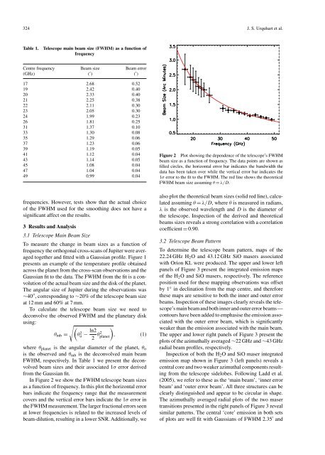
In Figure 2 we show the FWHM telescope beam sizes
as a function of frequency. In this plot the horizontal error
bars indicate the frequency range that the measurement
covers and the vertical error bars indicate the 1σ error in
the FWHM measurement. The larger fractional errors seen
at lower frequencies is related to the increased levels of
beam-dilution, resulting in a lower SNR. Additionally, we
Figure 2 Plot showing the dependence of the telescope’s FWHM
beam size as a function of frequency. The data points are shown as
filled circles, the horizontal error bar indicates the bandwidth the
data has been taken over while the vertical error bar indicates the
1σ error to the fit to the FWHM. The red line shows the theoretical
FWHM beam size assuming θ = λ/D.
also plot the theoretical beam sizes (solid red line), calculated
assuming θ = λ/D, where θ is measured in radians,
λ is the observed wavelength and D is the diameter of
the telescope. Inspection of the derived and theoretical
beams sizes reveals a strong correlation with a correlation
coefficient = 0.90.
3.2 Telescope Beam Pattern
To determine the telescope beam pattern, maps of the
22.24 GHz H2O and 43.12 GHz SiO masers associated
with Orion KL were produced. The upper and lower left
panels of Figure 3 present the integrated emission maps
of the H2O and SiO masers, respectively. The reference
position used for these mapping observations was offset
by 1◦ in declination from the map centre, and therefore
these maps are sensitive to both the inner and outer error
beams. Inspection of these images clearly reveals the telescope’s
main beam and both inner and outer error beams —
contours have been added to emphasise the emission associated
with the outer error beam, which is significantly
weaker than the emission associated with the main beam.
The upper and lower right panels of Figure 3 present the
plots of the azimuthally averaged ∼22 GHz and ∼43 GHz
radial beam profiles, respectively.
Inspection of both the H2O and SiO maser integrated
emission map shown in Figure 3 (left panels) reveals a
central core and two weaker azimuthal components resulting
from the telescope sidelobes. Following Ladd et al.
(2005), we refer to these as the ‘main beam’, ‘inner error
beam’ and ‘outer error beam’. All three structures can be
clearly distinguished and appear to be circular in shape.
The azimuthally averaged radial plots of the two maser
transitions presented in the right panels of Figure 3 reveal
similar patterns. The central ‘core’ emission in both sets
of plots are well fit with Gaussians of FWHM 2.35 ′ and