Grid diagrams in Heegaard Floer theory - UCLA Department of ...
Grid diagrams in Heegaard Floer theory - UCLA Department of ...
Grid diagrams in Heegaard Floer theory - UCLA Department of ...

Create successful ePaper yourself
Turn your PDF publications into a flip-book with our unique Google optimized e-Paper software.
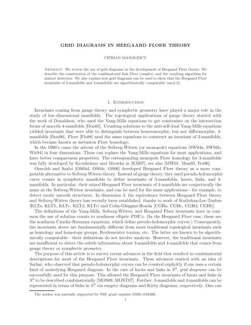
GRID DIAGRAMS IN HEEGAARD FLOER THEORY<br />
CIPRIAN MANOLESCU<br />
Abstract. We review the use <strong>of</strong> grid <strong>diagrams</strong> <strong>in</strong> the development <strong>of</strong> <strong>Heegaard</strong> <strong>Floer</strong> <strong>theory</strong>. We<br />
describe the construction <strong>of</strong> the comb<strong>in</strong>atorial l<strong>in</strong>k <strong>Floer</strong> complex, and the result<strong>in</strong>g algorithm for<br />
unknot detection. We also expla<strong>in</strong> how grid <strong>diagrams</strong> can be used to show that the <strong>Heegaard</strong> <strong>Floer</strong><br />
<strong>in</strong>variants <strong>of</strong> 3-manifolds and 4-manifolds are algorithmically computable (mod 2).<br />
1. Introduction<br />
Invariants com<strong>in</strong>g from gauge <strong>theory</strong> and symplectic geometry have played a major role <strong>in</strong> the<br />
study <strong>of</strong> low-dimensional manifolds. The topological applications <strong>of</strong> gauge <strong>theory</strong> started with<br />
the work <strong>of</strong> Donaldson, who used the Yang-Mills equations to get constra<strong>in</strong>ts on the <strong>in</strong>tersection<br />
forms <strong>of</strong> smooth 4-manifolds [Don83]. Count<strong>in</strong>g solutions to the anti-self-dual Yang-Mills equations<br />
yielded <strong>in</strong>variants that were able to dist<strong>in</strong>guish between homeomorphic, but not diffeomorphic, 4manifolds<br />
[Don90]. <strong>Floer</strong> [Flo88] used the same equations to construct an <strong>in</strong>variant <strong>of</strong> 3-manifolds,<br />
which became known as <strong>in</strong>stanton <strong>Floer</strong> homology.<br />
In the 1990’s came the advent <strong>of</strong> the Seiberg-Witten (or monopole) equations [SW94a, SW94b,<br />
Wit94] <strong>in</strong> four dimensions. These can replace the Yang-Mills equations for most applications, and<br />
have better compactness properties. The correspond<strong>in</strong>g monopole <strong>Floer</strong> homology for 3-manifolds<br />
was fully developed by Kronheimer and Mrowka <strong>in</strong> [KM07]; see also [MW01, Man03, Frø96].<br />
Ozsváth and Szabó [OS04d, OS04c, OS06] developed <strong>Heegaard</strong> <strong>Floer</strong> <strong>theory</strong> as a more computablealternativetoSeiberg-Witten<strong>theory</strong>.<br />
Instead<strong>of</strong>gauge<strong>theory</strong>, theyusedpseudo-holomorphic<br />
curve counts <strong>in</strong> symplectic manifolds to def<strong>in</strong>e <strong>in</strong>variants <strong>of</strong> 3-manifolds, knots, l<strong>in</strong>ks, and 4manifolds.<br />
In particular, their mixed <strong>Heegaard</strong> <strong>Floer</strong> <strong>in</strong>variants <strong>of</strong> 4-manifolds are conjecturally the<br />
same as the Seiberg-Witten <strong>in</strong>variants, and can be used for the same applications—for example, to<br />
detect exotic smooth structures. In dimension 3, the equivalence between <strong>Heegaard</strong> <strong>Floer</strong> <strong>theory</strong><br />
and Seiberg-Witten <strong>theory</strong> has recently been established, thanks to work <strong>of</strong> Kutluhan-Lee-Taubes<br />
[KLTa, KLTb, KLTc, KLTd, KLTe] and Col<strong>in</strong>-Ghigg<strong>in</strong>i-Honda [CGHa, CGHc, CGHd, CGHb].<br />
The def<strong>in</strong>itions <strong>of</strong> the Yang-Mills, Seiberg-Witten, and <strong>Heegaard</strong> <strong>Floer</strong> <strong>in</strong>variants have <strong>in</strong> common<br />
the use <strong>of</strong> solution counts to nonl<strong>in</strong>ear elliptic PDE’s. (In the <strong>Heegaard</strong> <strong>Floer</strong> case, these are<br />
the nonl<strong>in</strong>ear Cauchy-Riemann equations, which def<strong>in</strong>epseudo-holomorphic curves.) Consequently,<br />
the <strong>in</strong>variants above are fundamentally different from more traditional topological <strong>in</strong>variants such<br />
as homology and homotopy groups, Reidemeister torsion, etc. The latter are known to be algorithmically<br />
computable—their def<strong>in</strong>itions do not <strong>in</strong>volve analysis. However, the traditional <strong>in</strong>variants<br />
are <strong>in</strong>sufficient to detect the subtle <strong>in</strong>formation about 3-manifolds and 4-manifolds that comes from<br />
gauge <strong>theory</strong> or symplectic geometry.<br />
The purpose<strong>of</strong> this article is to survey recent advances <strong>in</strong> the field that resulted <strong>in</strong> comb<strong>in</strong>atorial<br />
descriptions for most <strong>of</strong> the <strong>Heegaard</strong> <strong>Floer</strong> <strong>in</strong>variants. These advances started with an idea <strong>of</strong><br />
Sarkar, whoobserved that pseudo-holomorphiccurves can becounted explicitly if one uses a certa<strong>in</strong><br />
k<strong>in</strong>d <strong>of</strong> underly<strong>in</strong>g <strong>Heegaard</strong> diagram. In the case <strong>of</strong> knots and l<strong>in</strong>ks <strong>in</strong> S 3 , grid <strong>diagrams</strong> can be<br />
successfully used for this purpose. This allowed the <strong>Heegaard</strong> <strong>Floer</strong> <strong>in</strong>variants <strong>of</strong> knots and l<strong>in</strong>ks <strong>in</strong><br />
S 3 tobedescribedcomb<strong>in</strong>atorially [MOS09,MOST07]. Further,3-manifoldsand4-manifoldscanbe<br />
represented <strong>in</strong> terms <strong>of</strong> l<strong>in</strong>ks <strong>in</strong> S 3 via surgery <strong>diagrams</strong> and Kirby <strong>diagrams</strong>, respectively. One can<br />
The author was partially supported by NSF grant number DMS-1104406.<br />
1
2 CIPRIAN MANOLESCU<br />
Y 3<br />
β1<br />
Uβ<br />
α1 α2 α3<br />
Uα<br />
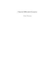
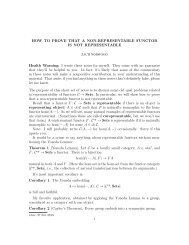
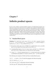
Figure 1. A marked <strong>Heegaard</strong> diagram for S 1 ×S 2 .<br />
then show that the <strong>Heegaard</strong> <strong>Floer</strong> <strong>in</strong>variants (modulo 2) <strong>of</strong> 3- and 4-manifolds are algorithmically<br />
computable, by express<strong>in</strong>g these <strong>in</strong>variants <strong>in</strong> terms <strong>of</strong> those <strong>of</strong> the correspond<strong>in</strong>g l<strong>in</strong>k [OS08b, MO,<br />
MOT].<br />
There are several alternate comb<strong>in</strong>atorial approaches to comput<strong>in</strong>g some <strong>of</strong> the <strong>Heegaard</strong> <strong>Floer</strong><br />
<strong>in</strong>variants. These approaches <strong>in</strong>clude nice <strong>diagrams</strong> [SW10, LMW08, OSS11], cubes <strong>of</strong> resolutions<br />
[OS09, BL], and bordered <strong>Floer</strong> homology [LOT]. In some cases, the result<strong>in</strong>g algorithms are<br />
more efficient than the ones based on grid <strong>diagrams</strong>. Nevertheless, grid <strong>diagrams</strong> are the most<br />
encompass<strong>in</strong>g method, and they are the focus <strong>of</strong> our survey.<br />
Acknowledgements. I owe an <strong>in</strong>tellectual debt to my collaborators Robert Lipshitz, Peter<br />
Ozsváth, Sucharit Sarkar, Zoltán Szabó, Dylan Thurston, and Jiajun Wang, who all played an<br />
important role <strong>in</strong> the development <strong>of</strong> the subject. I would also like to thank Tye Lidman for many<br />
helpful expository suggestions.<br />
2. <strong>Heegaard</strong> <strong>Floer</strong> homology and related <strong>in</strong>variants<br />
This section conta<strong>in</strong>s a quick overview <strong>of</strong> <strong>Heegaard</strong> <strong>Floer</strong> <strong>theory</strong>.<br />
The <strong>theory</strong> started with the work <strong>of</strong> Ozsváth and Szabó, who <strong>in</strong> [OS04d, OS04c] <strong>in</strong>troduced a<br />
set <strong>of</strong> 3-manifold <strong>in</strong>variants <strong>in</strong> the form <strong>of</strong> modules over the polynomial r<strong>in</strong>g Z[U]. Roughly, their<br />
construction goes as follows. We represent a closed, oriented 3-manifold Y by a marked <strong>Heegaard</strong><br />
diagram, consist<strong>in</strong>g <strong>of</strong> the follow<strong>in</strong>g data:<br />
• Σ, a closed oriented surface <strong>of</strong> genus g;<br />
• α = {α1,...,αg}, a collection <strong>of</strong> disjo<strong>in</strong>t, homologically l<strong>in</strong>early <strong>in</strong>dependent, simple closed<br />
curves on Σ. By attach<strong>in</strong>g g disks to Σ along the curves αi, and then attach<strong>in</strong>g a 3-ball,<br />
we obta<strong>in</strong> a handlebody Uα with boundary Σ;<br />
• β = {β1,...,βg} a similar collection <strong>of</strong> curves on Σ, specify<strong>in</strong>g a handlebody Uβ;<br />
• a basepo<strong>in</strong>t z ∈ Σ−∪αi −∪βi;<br />
suchthat Y = Uα∪ΣUβ. Any 3-manifold can berepresented<strong>in</strong> thisway; seeFigure1foraschematic<br />
picture.<br />
Next, we consider the tori<br />
β2<br />
β3<br />
Tα = α1 ×···×αg, Tβ = β1 ×···×βg<br />
<strong>in</strong>side the symmetric product Sym g (Σ) = (Σ ×··· ×Σ)/Sg, which can be viewed as a symplectic<br />
manifold, cf. [Per08]. After small perturbations <strong>of</strong> the alpha or beta curves, we can assume that<br />
Tα and Tβ <strong>in</strong>tersect transversely.<br />
To def<strong>in</strong>e the <strong>Heegaard</strong> <strong>Floer</strong> complex, we consider the <strong>in</strong>tersection po<strong>in</strong>ts<br />
x = {x1,...,xg} ∈ Tα ∩Tβ<br />
z<br />
Σ
GRID DIAGRAMS IN HEEGAARD FLOER THEORY 3<br />
with xi ∈ αi∩βj ⊂ Σ. Given two such <strong>in</strong>tersection po<strong>in</strong>ts x,y, a Whitney disk from x to y is def<strong>in</strong>ed<br />
to be a map u from the unit disk D 2 to Sym g (Σ), such that u maps the lower half <strong>of</strong> the boundary<br />
∂D 2 to Tα, the upper half to Tβ, and u(−1) = x,u(1) = y. The space <strong>of</strong> relative homotopy classes<br />
<strong>of</strong> Whitney disks from x to y is denoted π2(x,y). There is a natural map<br />
Tα ∩Tβ → Sp<strong>in</strong> c (Y), x → sz(x)<br />
send<strong>in</strong>g each <strong>in</strong>tersection po<strong>in</strong>t to a Sp<strong>in</strong> c structure on Y, such that π2(x,y) is empty when sz(x) �=<br />
sz(y).<br />
For every φ ∈ π2(x,y), we can consider the moduli space <strong>of</strong> pseudo-holomorphic disks <strong>in</strong> the<br />
class φ. These disks are solutions to the nonl<strong>in</strong>ear Cauchy-Riemann equations, which depend on<br />
the choice <strong>of</strong> a family J = {Jt} t∈[0,1] <strong>of</strong> almost complex structures on the symmetric product. The<br />
modulispacehasanexpecteddimensionµ(φ)(theMaslov <strong>in</strong>dex), anditcomes withanaturalaction<br />
<strong>of</strong> Rby automorphisms<strong>of</strong> thedoma<strong>in</strong>. Ifµ(φ) = 1, thenfor genericJ, after divid<strong>in</strong>gby theRaction<br />
the moduli space becomes just a f<strong>in</strong>ite set <strong>of</strong> po<strong>in</strong>ts, which can be counted with certa<strong>in</strong> signs. We<br />
let c(φ,J) ∈ Z denote the result<strong>in</strong>g count. Moreover, we denote by nz(φ) the <strong>in</strong>tersection number<br />
between φ and the divisor {z}×Sym g−1 (Σ). If φ admits any pseudo-holomorphic representatives,<br />
the pr<strong>in</strong>ciple <strong>of</strong> positivity <strong>of</strong> <strong>in</strong>tersections for holomorphic maps implies that nz(φ) ≥ 0.<br />
Fix a Sp<strong>in</strong> c structure s on Y. Under a certa<strong>in</strong> assumption on the <strong>Heegaard</strong> diagram (admissibility),<br />
one def<strong>in</strong>es the <strong>Heegaard</strong> <strong>Floer</strong> complex CF − (Y,s) to be the Z[U]-module freely generated<br />
by <strong>in</strong>tersection po<strong>in</strong>ts x ∈ Tα ∩Tβ with sz(x) = s. The differential on CF − (Y,s) is given by the<br />
formula:<br />
∂x =<br />
�<br />
�<br />
{y∈Tα∩Tβ|sz(y)=s} {φ∈π2(x,y)|µ(φ)=1}<br />
c(φ,J)·U nz(φ) y.<br />
It can be shown that ∂ 2 = 0. Start<strong>in</strong>g from the complex CF − = CF − (Y,s) one def<strong>in</strong>es the<br />
various versions <strong>of</strong> <strong>Heegaard</strong> <strong>Floer</strong> homology to be:<br />
HF − = H∗(CF − ), HF + = H∗(U −1 CF − /CF − ),<br />
HF ∞ = H∗(U −1 CF − ), � HF = H∗(CF − /(U = 0)).<br />
Although the complex CF − depends on the choices <strong>of</strong> <strong>Heegaard</strong> diagram and almost complex<br />
structure, the homology groups do not:<br />
Theorem 2.1 ([OS04d]). The <strong>Heegaard</strong> <strong>Floer</strong> homology modules HF − (Y,s), HF + (Y,s), HF ∞ (Y,s),<br />
�HF(Y,s) are <strong>in</strong>variants <strong>of</strong> the 3-manifold Y equipped with the Sp<strong>in</strong> c structure s.<br />
If ◦ is any <strong>of</strong> the four flavors <strong>of</strong> <strong>Heegaard</strong> <strong>Floer</strong> homology (−, +, ∞, or ∧), we will denote by<br />
HF ◦ (Y) the direct sum <strong>of</strong> HF ◦ (Y,s) over all Sp<strong>in</strong> c structures s.<br />
<strong>Heegaard</strong> <strong>Floer</strong> homology has found numerous applications to 3-dimensional topology. Among<br />
them we mention: detection <strong>of</strong> the Thurston norm [OS04a], detection <strong>of</strong> whether the 3-manifold<br />
fibers over the circle [Ni09], and a characterization <strong>of</strong> which Seifert fibrations admit tight contact<br />
structures [LS09].<br />
The reader may wonder about the differences between the different variants <strong>of</strong> <strong>Heegaard</strong> <strong>Floer</strong><br />
homology. The full power <strong>of</strong> the <strong>theory</strong> comes from the versions HF − and HF + , which conta<strong>in</strong><br />
(roughly) equivalent <strong>in</strong>formation. The version � HF is weaker: it suffices for many 3-dimensional applications,<br />
but it does not give any non-trivial <strong>in</strong>formation about closed 4-manifolds. (As expla<strong>in</strong>ed<br />
below, the mixed <strong>in</strong>variants <strong>of</strong> 4-manifolds are constructed by comb<strong>in</strong><strong>in</strong>g the plus and m<strong>in</strong>us theories.)<br />
The version HF ∞ is the least useful, be<strong>in</strong>g determ<strong>in</strong>ed by classical topological <strong>in</strong>formation,<br />
at least when we work modulo 2 and we restrict to torsion Sp<strong>in</strong> c structures; see [Lid].<br />
As proved by Ozsváth and Szabó <strong>in</strong> [OS06], the four variants <strong>of</strong> <strong>Heegaard</strong> <strong>Floer</strong> homology are<br />
functorial under Sp<strong>in</strong> c -decorated cobordisms. Precisely, given a 4-dimensional manifold W with
4 CIPRIAN MANOLESCU<br />
∂W = (−Y0)∪Y1, and a Sp<strong>in</strong> c structure s on W with restrictions s0 to Y0 and s1 to Y1, there are<br />
<strong>in</strong>duced maps:<br />
F ◦ W,s : HF◦ (Y0,s0) −→ HF ◦ (Y1,s1),<br />
where ◦ can stand for any <strong>of</strong> the four flavors <strong>of</strong> <strong>Heegaard</strong> <strong>Floer</strong> homology. The maps F ◦ W,s are<br />
def<strong>in</strong>ed by count<strong>in</strong>g pseudo-holomorphic triangles <strong>in</strong> the symmetric product, with boundaries on<br />
three different tori.<br />
Suppose we have a smooth, closed, oriented 4-manifold X with b + 2 (X) > 1. An admissible cut<br />
for X is a smoothly embedded 3-manifold N ⊂ X which divides X <strong>in</strong>to two pieces X1 and X2 with<br />
b + 2 (Xi) > 0 for i = 1,2, and such that δH1 (N;Z) = 0 ⊂ H2 (X;Z).<br />
An admissible cut can be found for any X. Given an admissible cut, one can delete a four-ball<br />
from the <strong>in</strong>terior <strong>of</strong> each piece Xi to obta<strong>in</strong> two cobordisms W1 (from S3 to N) and W2 (from N<br />
to S3 ). Let s be a Sp<strong>in</strong>c structure on X. We consider the follow<strong>in</strong>g diagram:<br />
HF− (S3 F<br />
)<br />
−<br />
W1 ,s| W1<br />
��<br />
HF<br />
❚ ❚ ❚ ❚ ❚ ❚ ❚ ❚��<br />
− (N,s|N)<br />
��<br />
� �<br />
HFred(N,s|N)<br />
❚ ❚ ❚ ❚ ❚ ❚ ❚ ❚��<br />
HF + ����<br />
(N,s|N)<br />
��<br />
+ HF (S3 ),<br />
F +<br />
W 2 ,s| W2<br />
where HFred is the image <strong>of</strong> a natural map HF + → HF − . (This map exists for any 3-manifold.)<br />
The conditions <strong>in</strong> the def<strong>in</strong>ition <strong>of</strong> an admissible cut ensure that the maps F −<br />
W1,s|W 1<br />
and F +<br />
W2,s|W 2<br />
factor through HFred. The composition <strong>of</strong> the two lifts (<strong>in</strong>dicated by dashed arrrows) is called<br />
a mixed map. The image <strong>of</strong> 1 ∈ HF − (S 3 ) ∼ = Z under this map def<strong>in</strong>es the Ozsváth-Szabó mixed<br />
<strong>in</strong>variant <strong>of</strong> the pair (X,s). This is conjecturally equivalent to the well-known Seiberg-Witten<br />
<strong>in</strong>variant [Wit94], and is known to share many <strong>of</strong> its properties. In particular, it can be used to<br />
dist<strong>in</strong>guish homeomorphic 4-manifolds that are not diffeomorphic.<br />
3. L<strong>in</strong>k <strong>Floer</strong> homology<br />
Ozsváth-Szabó [OS04b] and, <strong>in</strong>dependently, Rasmussen [Ras03] used <strong>Heegaard</strong> <strong>Floer</strong> <strong>theory</strong> to<br />
def<strong>in</strong>e <strong>in</strong>variants for knots <strong>in</strong> 3-manifolds: these are the various versions <strong>of</strong> knot <strong>Floer</strong> homology.<br />
Recall that a marked <strong>Heegaard</strong> diagram (Σ,α,β,z) represents a 3-manifold Y. If one specifies<br />
another basepo<strong>in</strong>t w <strong>in</strong> the complement <strong>of</strong> the alpha and beta curves, this gives rise to a knot<br />
K ⊂ Y. Indeed, one can jo<strong>in</strong> w to z by a path <strong>in</strong> Σ\∪αi, and then push this path <strong>in</strong>to the <strong>in</strong>terior<br />
<strong>of</strong> the handlebody Uα. Similarly, one can jo<strong>in</strong> w to z <strong>in</strong> the complement <strong>of</strong> the beta curves, and<br />
push the path <strong>in</strong>to Uβ. The union <strong>of</strong> these two paths is the knot K. For simplicity, we will assume<br />
that K is null-homologous. (Of course, this happens automatically if Y = S 3 .)<br />
In the def<strong>in</strong>ition <strong>of</strong> the <strong>Heegaard</strong> <strong>Floer</strong> complex CF − we kept track <strong>of</strong> <strong>in</strong>tersections with z<br />
through the exponent nz(φ) <strong>of</strong> the variable U. Now that we have two basepo<strong>in</strong>ts, we have two<br />
quantities nz(φ) and nw(φ). One th<strong>in</strong>g we can do is to count only disks <strong>in</strong> classes with nz(φ) = 0,<br />
and keep track <strong>of</strong> nw(φ) <strong>in</strong> the exponent <strong>of</strong> U. The result is a complex <strong>of</strong> Z[U]-modules denoted<br />
CFK − (Y,K), with homology HFK − (Y,K). If we set the variable U to zero, we get a complex<br />
�CFK(Y,K), with homology �HFK(Y,K). These are two <strong>of</strong> the variants <strong>of</strong> knot <strong>Floer</strong> homology.<br />
There exist many other variants, some <strong>of</strong> which <strong>in</strong>volve classes φ with nz(φ) �= 0 and nw(φ) �= 0;<br />
an example <strong>of</strong> this, denoted A ± (K), will be mentioned <strong>in</strong> section 5.
GRID DIAGRAMS IN HEEGAARD FLOER THEORY 5<br />
Let us focus on the case when Y = S3 . The groups �HFK(S 3 ,K) naturally split as direct sums:<br />
�HFK(S 3 ,K) = �<br />
�HFKm(S 3 ,K,s).<br />
m,s∈Z<br />
Here, m and s are certa<strong>in</strong> quantities called the Maslov and Alexander grad<strong>in</strong>gs, respectively. We<br />
can encode some <strong>of</strong> the <strong>in</strong>formation <strong>in</strong> �HFK <strong>in</strong>to a polynomial<br />
PK(t,q) = �<br />
m,s∈Z<br />
t m q s ·rank �HFKm(S 3 ,K,s).<br />
The specialization PK(−1,q) is the classical Alexander polynomial <strong>of</strong> K. However, the applications<br />
<strong>of</strong> knot <strong>Floer</strong> homology go well beyond those <strong>of</strong> the Alexander polynomial. In particular, the<br />
genus <strong>of</strong> the knot, which is def<strong>in</strong>ed as<br />
can be read from �HFK:<br />
g(K) = m<strong>in</strong>{g | ∃ embedded, oriented surfaceΣ ⊂ S 3 , ∂Σ = K},<br />
Theorem 3.1 ([OS04a]). For any knot K ⊂ S 3 , we have<br />
g(K) = max{s ≥ 0 | ∃ m, �HFKm(S 3 ,K,s) �= 0}.<br />
S<strong>in</strong>ce the only knot <strong>of</strong> genus zero is the unknot, we have:<br />
Corollary 3.2. K is the unknot if and only if PK(q,t) = 1.<br />
By a result <strong>of</strong> Ghigg<strong>in</strong>i [Ghi08], the polynomial P has enough <strong>in</strong>formation to also detect the<br />
right-handed trefoil, the left-handed trefoil, and the figure-eight knot. Ni [Ni07] extended the work<br />
<strong>in</strong> [Ghi08] to show that S 3 \ K fibers over the circle if and only if ⊕m �HFKm(S 3 ,K,g(K)) ∼ = Z.<br />
Other applications <strong>of</strong> knot <strong>Floer</strong> homology <strong>in</strong>clude the construction <strong>of</strong> a concordance <strong>in</strong>variant<br />
called τ [OS03], and a complete characterization <strong>of</strong> which lens spaces can be obta<strong>in</strong>ed by surgery<br />
on knots [Gre].<br />
If <strong>in</strong>stead <strong>of</strong> a knot K ⊂ S 3 we have a l<strong>in</strong>k L (a disjo<strong>in</strong>t union <strong>of</strong> knots), we can def<strong>in</strong>e <strong>in</strong>variants<br />
�HFL(S 3 ,L),HFL − (S 3 ,L), which are versions <strong>of</strong> l<strong>in</strong>k <strong>Floer</strong> homology. When L is a knot, �HFL<br />
and HFL − reduce to �HFK and HFK − , respectively. In general, the def<strong>in</strong>ition <strong>of</strong> l<strong>in</strong>k <strong>Floer</strong><br />
homology <strong>in</strong>volves choos<strong>in</strong>g a new k<strong>in</strong>d <strong>of</strong> <strong>Heegaard</strong> diagram for S 3 , <strong>in</strong> which the number <strong>of</strong> alpha<br />
(or beta) curves exceeds the genus <strong>of</strong> the <strong>Heegaard</strong> surface. The details can be found <strong>in</strong> [OS08a].<br />
If the diagram has g +k −1 alpha curves, it should also have g +k −1 beta curves, k basepo<strong>in</strong>ts<br />
<strong>of</strong> type z, and k basepo<strong>in</strong>ts <strong>of</strong> type w. In the simplest version, k is the same as the number ℓ <strong>of</strong><br />
components <strong>of</strong> the l<strong>in</strong>k, and jo<strong>in</strong><strong>in</strong>g the w basepo<strong>in</strong>ts to the z basepo<strong>in</strong>ts <strong>in</strong> pairs (by a total <strong>of</strong> 2ℓ<br />
paths) produces the l<strong>in</strong>k L. Instead <strong>of</strong> Z[U], the l<strong>in</strong>k <strong>Floer</strong> complexes are def<strong>in</strong>ed over a polynomial<br />
r<strong>in</strong>g Z/2[U1,...,Uℓ], with one variable for each component. (In fact, we expect the complexes to<br />
be def<strong>in</strong>ed over Z[U1,...,Uℓ]. However, at the moment some orientation issues are not yet settled,<br />
and the <strong>theory</strong> is only def<strong>in</strong>ed with mod 2 coefficients.)<br />
More generally, we could have k ≥ ℓ, and break the l<strong>in</strong>k <strong>in</strong>to more segments. We can then def<strong>in</strong>e<br />
a l<strong>in</strong>k <strong>Floer</strong> complex over Z/2[U1,...,Uk], with one variable for each basepo<strong>in</strong>t; see [MOS09, MO].<br />
The homology <strong>of</strong> this complex is still HFL − , and all the variables correspond<strong>in</strong>g to basepo<strong>in</strong>ts on<br />
the same l<strong>in</strong>k component act the same way. If we set one Ui variable from each l<strong>in</strong>k component to<br />
zero <strong>in</strong> the complex, the result<strong>in</strong>g homology is �HFL. If we set all the Ui variables to zero <strong>in</strong> the<br />
complex, the homology becomes<br />
(1)<br />
�HFL(S 3 ,L)⊗V k−ℓ ,<br />
where V is a two-dimensional vector space over Z/2.
6 CIPRIAN MANOLESCU<br />
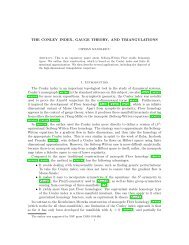
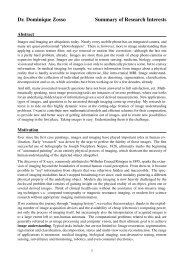
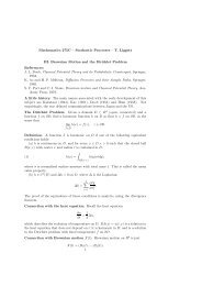
Figure 2. A grid diagram for the trefoil, and two empty rectangles <strong>in</strong> Rect ◦ (x,y).<br />
Here, x is <strong>in</strong>dicated by the collection <strong>of</strong> black dots, and y by the collection <strong>of</strong> white<br />
dots. One empty rectangle is darkly shaded. The other rectangle is wrapped around<br />
the torus, and consists <strong>of</strong> the union <strong>of</strong> the four lightly shaded areas.<br />
4. <strong>Grid</strong> <strong>diagrams</strong> and comb<strong>in</strong>atorial l<strong>in</strong>k <strong>Floer</strong> complexes<br />
Def<strong>in</strong>ition 4.1. Let L ⊂ S 3 be a l<strong>in</strong>k. A grid diagram for L consists <strong>of</strong> an n-by-n grid <strong>in</strong> the plane<br />
with O and X mark<strong>in</strong>gs <strong>in</strong>side, such that:<br />
(1) Each row and each column conta<strong>in</strong>s exactly one X and one O;<br />
(2) As we trace the vertical and horizontal segments between O’s and X’s (with the vertical<br />
segments pass<strong>in</strong>g over the horizontal segments), we see a planar diagram for the l<strong>in</strong>k L.<br />
An example is shown on the left hand side <strong>of</strong> Figure 2. It is not hard to see that every l<strong>in</strong>k<br />
admits a grid diagram. In fact, as a way <strong>of</strong> represent<strong>in</strong>g l<strong>in</strong>ks, grid <strong>diagrams</strong> are equivalent to arc<br />
presentations, which orig<strong>in</strong>ated <strong>in</strong> the work <strong>of</strong> Brunn [Bru98]. The m<strong>in</strong>imal number n such that L<br />
admits a grid diagram <strong>of</strong> size n is called the arc <strong>in</strong>dex <strong>of</strong> L.<br />
<strong>Grid</strong> <strong>diagrams</strong> can be viewed as particular examples <strong>of</strong> <strong>Heegaard</strong> <strong>diagrams</strong> with multiple basepo<strong>in</strong>ts,<br />
<strong>of</strong> the k<strong>in</strong>d discussed at the end <strong>of</strong> the previous section. Indeed, if we identify the opposite<br />
sides <strong>of</strong> a grid diagram G to get a torus, we can let this torus be the <strong>Heegaard</strong> surface Σ, the<br />
horizontal circles be the α curves, the vertical circles be the β curves, the O mark<strong>in</strong>gs be the w<br />
basepo<strong>in</strong>ts, and the X mark<strong>in</strong>gs be the z basepo<strong>in</strong>ts. A po<strong>in</strong>t x = {x1,...,xn} <strong>in</strong> the <strong>in</strong>tersection<br />
Tα∩Tβ consists an n-tuple <strong>of</strong> po<strong>in</strong>ts on the grid (one on each vertical and horizontal circle). There<br />
are n! such <strong>in</strong>tersection po<strong>in</strong>ts, and they are precisely the generators <strong>of</strong> the l<strong>in</strong>k <strong>Floer</strong> complex. We<br />
denote the set <strong>of</strong> these generators by S(G).<br />
Def<strong>in</strong>ition 4.2. Let G be a grid diagram, and x,y ∈ S(G). We def<strong>in</strong>e a rectangle from x to y to<br />
be a rectangle on the grid torus with the lower left and upper right corner be<strong>in</strong>g po<strong>in</strong>ts <strong>of</strong> x, the<br />
lower right and upper right corners be<strong>in</strong>g po<strong>in</strong>ts <strong>of</strong> y, and such that all the other components <strong>of</strong> x<br />
and y co<strong>in</strong>cide. (In particular, for such a rectangle to exist we need x to differ from y <strong>in</strong> exactly<br />
two rows.) A rectangle is called empty if it conta<strong>in</strong>s no components <strong>of</strong> x or y <strong>in</strong> its <strong>in</strong>terior. The<br />
set <strong>of</strong> empty rectangles from x to y is denoted Rect ◦ (x,y).<br />
Of course, the space Rect ◦ (x,y) has at most two elements. An example where it has exactly two<br />
is shown on the right hand side <strong>of</strong> Figure 2.<br />
The reason why grid <strong>diagrams</strong> are useful <strong>in</strong> <strong>Heegaard</strong> <strong>Floer</strong> <strong>theory</strong> is that they make pseudoholomorphic<br />
disks <strong>of</strong> Maslov <strong>in</strong>dex 1 easy to count:<br />
Proposition 4.3 ([MOS09]). Let G be a grid diagram, and let x,y ∈ S(G). Then, there is a 1-to-1<br />
correspondence:<br />
�<br />
�<br />
φ ∈ π2(x,y) | µ(φ) = 1, c(φ,J) ≡ 1(mod 2) for generic J ←→ Rect ◦ (x,y).
GRID DIAGRAMS IN HEEGAARD FLOER THEORY 7<br />
Sketch <strong>of</strong> pro<strong>of</strong>. In any <strong>Heegaard</strong> diagram, if we have a relative homotopy class φ ∈ π2(x,y), we<br />
can associate to it a two-cha<strong>in</strong> D(φ) on the <strong>Heegaard</strong> surface Σ, as follows. Let n be the number<br />
<strong>of</strong> alpha (or beta) curves. Together, the alpha and the beta curves split Σ <strong>in</strong>to several connected<br />
regions R1,...,Rm. For each i, let us pick a po<strong>in</strong>t pi <strong>in</strong> the <strong>in</strong>terior <strong>of</strong> Ri, and def<strong>in</strong>ethe multiplicity<br />
<strong>of</strong> φ at Ri to be the <strong>in</strong>tersection number npi (φ) between φ and {pi}×Sym n−1 (φ). We set<br />
D(φ) = �<br />
npi (φ)Ri.<br />
i<br />
This is called the doma<strong>in</strong> <strong>of</strong> φ. If φ admits any pseudo-holomorphic representatives, then the<br />
multiplicities npi (φ) must be nonnegative.<br />
Lipshitz [Lip06] showed that the Maslov <strong>in</strong>dex <strong>of</strong> φ can be expressed <strong>in</strong> terms <strong>of</strong> the doma<strong>in</strong>:<br />
µ(φ) = e(D(φ))+N(D(φ)),<br />
where e and N are certa<strong>in</strong> quantities called the Euler measure and total vertex multiplicity, respectively.<br />
The Euler measure is additive on regions, that is, we can def<strong>in</strong>e e(Ri) such that<br />
e(D(φ)) = �<br />
<strong>in</strong>pi (φ)e(Ri). If we take the sum �<br />
ie(Ri) we get the Euler characteristic <strong>of</strong> the<br />
<strong>Heegaard</strong> surface Σ. As for the total vertex multiplicity, it is the sum <strong>of</strong> 2n vertex multiplicities<br />
Nq(D(φ)), one for each po<strong>in</strong>t q ∈ x or q ∈ y. The quantity Nq(D(φ)) is the average <strong>of</strong> the<br />
multiplicities <strong>of</strong> φ <strong>in</strong> the four quadrants around q.<br />
In the case <strong>of</strong> a grid G, the regions Ri are the n2 unit squares <strong>of</strong> G. Each square has Euler<br />
measure zero. If we have φ ∈ π2(x,y) with µ(φ) = 1 and c(φ,J) �= 0, then the coefficients <strong>of</strong> Ri<br />
<strong>in</strong> D(φ) are nonnegative. This implies that 1 = µ(φ) = N(D(φ)) is a sum <strong>of</strong> vertex multiplicities<br />
Nq(D(φ)). Each Nq(D(φ)) is either zero or at least 1/4. A short analysis shows that D(φ) must be<br />
an empty rectangle.<br />
Conversely, given an empty rectangle, there is a correspond<strong>in</strong>g class φ with µ(φ) = 1. An application<br />
<strong>of</strong> the Riemann mapp<strong>in</strong>g theorem shows that φ has an odd number <strong>of</strong> pseudo-holomorphic<br />
representatives for generic J. �<br />
In view <strong>of</strong> Proposition 4.3, the l<strong>in</strong>k <strong>Floer</strong> complex associated to a grid can be def<strong>in</strong>ed <strong>in</strong> a<br />
purely comb<strong>in</strong>atorial way. Precisely, we def<strong>in</strong>e C − (G) to be freely generated by S(G) over the r<strong>in</strong>g<br />
Z/2[U1,...,Un], with differential:<br />
∂x = �<br />
�<br />
y∈S(G) {r∈Rect◦ U<br />
(x,y)|Xi(r)=0, ∀i}<br />
O1(r)<br />
1 ...U On(r)<br />
n ·y.<br />
Here, Oi(r) encodes whether or not the i th mark<strong>in</strong>g <strong>of</strong> type O is <strong>in</strong> the <strong>in</strong>terior <strong>of</strong> the rectangle<br />
r: if it is, we set Oi(r) to be 1; otherwise it is 0. The quantity Xi(r) ∈ {0,1} is def<strong>in</strong>ed similarly,<br />
<strong>in</strong> terms <strong>of</strong> the i th mark<strong>in</strong>g <strong>of</strong> type X.<br />
The homology <strong>of</strong> C − (G) is the l<strong>in</strong>k <strong>Floer</strong> homology HFL − (S 3 ,L).<br />
Remark 4.4. Although the complex C − (G) is def<strong>in</strong>ed with mod 2 coefficients, one can add signs<br />
<strong>in</strong> the differential to get a complex over Z[U1,...,Un], whose homology is still a l<strong>in</strong>k <strong>in</strong>variant. See<br />
[MOST07, Gal08].<br />
If <strong>in</strong> C − (G) we set one variable Ui from each l<strong>in</strong>k component to zero, we get a complex � C(G)<br />
with homology �HFL(S 3 ,L). Perhaps the simplest complex is<br />
�C(G) = C − (G)/(U1 = U2 = ··· = Un = 0),<br />
for which we only need to count the empty rectangles with no mark<strong>in</strong>gs <strong>of</strong> any type <strong>in</strong> their <strong>in</strong>terior.<br />
The homology <strong>of</strong> � C(G) is �HFL(S 3 ,L)⊗V n−ℓ ; compare (1).<br />
In particular, when L = K is a knot, the homology <strong>of</strong> � C(G) is �HFK(S 3 ,K)⊗V n−1 . There exist<br />
simple comb<strong>in</strong>atorial formulas for the Maslov and Alexander grad<strong>in</strong>gs <strong>of</strong> the generators <strong>in</strong> S(G),<br />
and from them one gets a bi-grad<strong>in</strong>g on H∗( � C(G)); see [MOS09], [MOST07]. From here one can
8 CIPRIAN MANOLESCU<br />
recover �HFK(S 3 ,K) as a bi-graded group, tak<strong>in</strong>g <strong>in</strong>to account that each V factor is spanned by<br />
one generator <strong>in</strong> bi-degree (0,0) and another <strong>in</strong> bi-degree (−1,−1). This method <strong>of</strong> calculat<strong>in</strong>g<br />
�HFK was implemented on the computer by Baldw<strong>in</strong> and Gillam [BG]; see also Droz [Dro08] for a<br />
more efficient program, us<strong>in</strong>g a variation <strong>of</strong> this method due to Beliakova [Bel10].<br />
In view <strong>of</strong> Theorem 3.1, we see that grid <strong>diagrams</strong> yield an algorithm for detect<strong>in</strong>g the genus <strong>of</strong><br />
a knot. In particular, if we are given a knot diagram and want to see if it represents the unknot,<br />
we can turn it <strong>in</strong>to a grid diagram (after some suitable isotopies), then set up the complex � C(G),<br />
and check if H∗( � C(G)) ∼ = V n−1 .<br />
Among the other applications <strong>of</strong> the grid diagram method we mention one to contact geometry:<br />
the construction <strong>of</strong> new <strong>in</strong>variants for Legendrian and transverse knots <strong>in</strong> S 3 [OST08]. This led to<br />
numerous examples <strong>of</strong> transverse knots with the same self-l<strong>in</strong>k<strong>in</strong>g number that are not transversely<br />
isotopic [NOT08].<br />
Another application <strong>of</strong> knot <strong>Floer</strong> homology via grid <strong>diagrams</strong> is Sarkar’s comb<strong>in</strong>atorial pro<strong>of</strong><br />
<strong>of</strong> the Milnor conjecture [Sar]. The Milnor conjecture states that the slice genus <strong>of</strong> the torus knot<br />
T(p,q) is (p−1)(q −1)/2; a corollary is that the m<strong>in</strong>imum number <strong>of</strong> cross<strong>in</strong>g changes needed to<br />
turn T(p,q) <strong>in</strong>to the unknot is also (p−1)(q−1)/2. The conjecture was first proved by Kronheimer<br />
and Mrowka us<strong>in</strong>g gauge <strong>theory</strong> [KM93]; for other pro<strong>of</strong>s, see [OS03], [Ras10].<br />
Slight variations <strong>of</strong> grid <strong>diagrams</strong> can be used to compute the knot <strong>Floer</strong> homology <strong>of</strong> knots<br />
<strong>in</strong>side lens spaces [BGH08], and <strong>of</strong> a knot <strong>in</strong>side its cyclic branched covers [Lev08].<br />
F<strong>in</strong>ally, wementionthatthereexistsapurelycomb<strong>in</strong>atorial pro<strong>of</strong>thatH∗(C − (G))andH∗( � C(G))<br />
are l<strong>in</strong>k <strong>in</strong>variants [MOST07].<br />
5. Three-manifolds and four-manifolds<br />
For a general <strong>Heegaard</strong> diagram, count<strong>in</strong>g pseudo-holomorphic disks <strong>in</strong> the symmetric product<br />
is very difficult. Why is it easy for a grid diagram? If we look at the pro<strong>of</strong> <strong>of</strong> Proposition 4.3, a<br />
key po<strong>in</strong>t we f<strong>in</strong>d is that the regions Ri have zero Euler measure. In fact, what is important is that<br />
they have nonnegative Euler measure: s<strong>in</strong>ce the total vertex multiplicity is always nonnegative, the<br />
fact that e(D(φ))+N(D(φ)) = 1 imposes tight constra<strong>in</strong>ts on the possibilities for D(φ).<br />
In general, if a <strong>Heegaard</strong> surface Σ can be partitioned <strong>in</strong>to regions <strong>of</strong> nonnegative Euler measure,<br />
its Euler characteristic (which is the sum <strong>of</strong> all the Euler measures) must be nonnegative; that is,<br />
Σ must be a sphere or a torus. Our grid <strong>diagrams</strong> were set on a torus. There is also a variant<br />
on the sphere, that produces another comb<strong>in</strong>atorial l<strong>in</strong>k <strong>Floer</strong> complex, and <strong>in</strong> the end yields the<br />
same homology.<br />
Instead <strong>of</strong> a knot <strong>in</strong> S 3 , we could take a 3-manifold Y and try to compute its <strong>Heegaard</strong> <strong>Floer</strong><br />
homology us<strong>in</strong>g this method. The problem is that a typical 3-manifold does not admit a <strong>Heegaard</strong><br />
diagram <strong>of</strong> genus 0 or 1; only S 3 , S 1 ×S 2 and lens spaces do. However, Sarkar and Wang [SW10]<br />
proved that one can f<strong>in</strong>d a <strong>Heegaard</strong> diagram for Y, called a nice diagram, <strong>in</strong> which all regions<br />
except one have nonnegative Euler measure. (This is related to the fact that on a surface <strong>of</strong> higher<br />
genus we can move all negative curvatureto aneighborhood<strong>of</strong> a po<strong>in</strong>t.) Ifwe putthe basepo<strong>in</strong>tz <strong>in</strong><br />
the bad region (the one with negative Euler measure), then we can understand pseudo-holomorphic<br />
curve counts for all classes φ with nz(φ) = 0. These are the only classes that appear when def<strong>in</strong><strong>in</strong>g<br />
the complex � CF(Y). Thus, we get an algorithm for comput<strong>in</strong>g � HF <strong>of</strong> any 3-manifold. We refer to<br />
[SW10] for more details, and to [OSS11, OSS] for related work.<br />
Similarly, one can compute the cobordism maps ˆ FW,s for any simply connected W [LMW08].<br />
These suffice to detect exotic smooth structures on some 4-manifolds with boundary, but not on<br />
any closed 4-manifolds.<br />
This l<strong>in</strong>e <strong>of</strong> thought runs <strong>in</strong>to major difficulties if one wants to understand comb<strong>in</strong>atorially the<br />
plus and m<strong>in</strong>us versions <strong>of</strong> HF, or the mixed <strong>in</strong>variants <strong>of</strong> 4-manifolds. Instead, what is helpful is
GRID DIAGRAMS IN HEEGAARD FLOER THEORY 9<br />
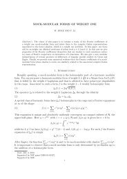
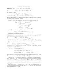
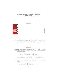
S 1 ×S 3<br />
0 0 1<br />
S 2 ×S 2 CP 2<br />
Figure 3. Kirby <strong>diagrams</strong> for a few simple 4-manifolds.<br />
to reduce everyth<strong>in</strong>g to the case <strong>of</strong> l<strong>in</strong>ks <strong>in</strong> S 3 , and then appeal to grid <strong>diagrams</strong>. This program<br />
was developed <strong>in</strong> [MO, MOT], and is summarized below.<br />
Let us recall a theorem <strong>of</strong> Lickorish and Wallace [Lic62, Wal60], which says that any closed<br />
3-manifold Y is <strong>in</strong>tegral surgery on a l<strong>in</strong>k <strong>in</strong> S 3 :<br />
Y = (S 3 \ν(L))∪φ (ν(L)).<br />
Here, ν(L) is a tubular neighborhood, and φ is a self-diffeomorphism <strong>of</strong> ∂ν(L). The diffeomorphism<br />
can be specified <strong>in</strong> terms <strong>of</strong> a fram<strong>in</strong>g <strong>of</strong> the l<strong>in</strong>k, which <strong>in</strong> turn is determ<strong>in</strong>ed by choos<strong>in</strong>g one<br />
<strong>in</strong>teger for each l<strong>in</strong>k component. For example, the Po<strong>in</strong>caré sphere is surgery on the right-handed<br />
trefoil with +1 fram<strong>in</strong>g. In general, we denote by S 3 Λ<br />
(L) the result <strong>of</strong> surgery on L with fram<strong>in</strong>g Λ.<br />
Four-manifolds can also be expressed <strong>in</strong> terms <strong>of</strong> l<strong>in</strong>ks, us<strong>in</strong>g Kirby <strong>diagrams</strong> [Kir78]. By Morse<br />
<strong>theory</strong>, a closed 4-manifold can be broken <strong>in</strong>to a 0-handle, some 1-handles (represented <strong>in</strong> a Kirby<br />
diagram by circles marked with a dot), some 2-handles (represented by framed knots), some 3handles,<br />
and a 4-handle. The positions <strong>of</strong> the 1-handles and 2-handles determ<strong>in</strong>e the manifold. See<br />
Figure 3 for a few examples.<br />
The next step <strong>in</strong> the program is to express the <strong>Heegaard</strong> <strong>Floer</strong> homology <strong>of</strong> surgery on a l<strong>in</strong>k <strong>in</strong><br />
terms <strong>of</strong> data associated to the l<strong>in</strong>k. The first result <strong>in</strong> this direction was obta<strong>in</strong>ed by Ozsváth and<br />
Szabó [OS08b], who dealt with surgery on knots:<br />
Theorem 5.1 ([OS08b]). There is an (<strong>in</strong>f<strong>in</strong>itely generated) version <strong>of</strong> the knot <strong>Floer</strong> complex,<br />
A + (K), such that<br />
HF + (S 3 � � + Φ<br />
n(K)) = H∗ Cone A (K) K �� n +<br />
−−→ A (∅)<br />
where <strong>in</strong> A + (K),A + (∅) we count pseudo-holomorphic bigons and <strong>in</strong> ΦK n we count pseudo-holomorphic<br />
triangles.<br />
The complex A + (∅) is a direct sum <strong>of</strong> <strong>in</strong>f<strong>in</strong>itely many copies <strong>of</strong> CF + (S3 ). The <strong>in</strong>clusion <strong>of</strong> one<br />
<strong>of</strong> these copies <strong>in</strong>to the mapp<strong>in</strong>g cone complex<br />
Cone � A + (K) ΦK � n +<br />
−−→ A (∅)<br />
<strong>in</strong>duces on homology the map F −<br />
W,s : HF+ (S3 ) −→ HF + (S3 n (K)) correspond<strong>in</strong>g to the surgery<br />
cobordism (2-handle attachment along K), equipped with a Sp<strong>in</strong>c structure s.<br />
The pro<strong>of</strong> <strong>of</strong> Theorem 5.1 is based on an important property <strong>of</strong> HF + called the surgery exact<br />
triangle. The version HF − does not have a similar exact triangle, but a slight variant <strong>of</strong> it, HF −<br />
does. The version HF − is obta<strong>in</strong>ed from HF − by completion with respect to the U variable. For<br />
torsion Sp<strong>in</strong> c structures s, one can recover HF − (Y,s) from HF − (Y,s), so <strong>in</strong> that case the two<br />
versions conta<strong>in</strong> equivalent <strong>in</strong>formation.<br />
There is an analogue <strong>of</strong> Theorem 5.1 with HF − <strong>in</strong>stead <strong>of</strong> HF + , and with a knot <strong>Floer</strong> complex<br />
denoted A − <strong>in</strong>stead <strong>of</strong> A + .<br />
There is also an extension <strong>of</strong> Theorem 5.1 to surgeries on l<strong>in</strong>ks rather than s<strong>in</strong>gle knots. Phrased<br />
<strong>in</strong> terms <strong>of</strong> HF − , it reads:
10 CIPRIAN MANOLESCU<br />
Theorem 5.2 ([MO]). If L = K1 ∪ K2 ⊂ S3 is a l<strong>in</strong>k with fram<strong>in</strong>g Λ, then HF− (S3 Λ (L)) is<br />
isomorphic to the homology <strong>of</strong> a complex C− (L,Λ) <strong>of</strong> the form<br />
(2) A− (L) ��<br />
A<br />
❑❑❑❑❑❑<br />
❑❑<br />
��<br />
❑❑��<br />
− (K1)<br />
��<br />
A− (K2) ��<br />
A− (∅)<br />
where the edge maps count holomorphic triangles, and the diagonal map counts holomorphic quadrilaterals.<br />
This can be generalized to l<strong>in</strong>ks with any number <strong>of</strong> components. The higher diagonals <strong>in</strong>volve<br />
count<strong>in</strong>g higher holomorphic polygons. Further, the <strong>in</strong>clusion <strong>of</strong> the subcomplex correspond<strong>in</strong>g to<br />
L ′ ⊆ L corresponds to the cobordism maps given by surgery on L−L ′ .<br />
Remark 5.3. For technical reasons, at the moment Theorem 5.2 is only established with mod 2<br />
coefficients.<br />
If W is a cobordism between (connected) 3-manifolds that consists <strong>of</strong> 2-handles only, then we<br />
can express one boundary piece <strong>of</strong> W as surgery on a l<strong>in</strong>k L ′ ⊂ S 3 , and W as a handle attachment<br />
along a l<strong>in</strong>k L−L ′ . Thus, Theorem 5.2 gives a description <strong>of</strong> the maps on HF − associated to any<br />
such cobordism W. In fact, 2-handles are the ma<strong>in</strong> source <strong>of</strong> complexity <strong>in</strong> 4-manifolds. Once we<br />
understand them, it is not hard to <strong>in</strong>corporate the maps <strong>in</strong>duced by 1-handles and 3-handles <strong>in</strong>to<br />
the picture. The result is a description <strong>of</strong> the Ozsváth-Szabó mixed <strong>in</strong>variant <strong>of</strong> a 4-manifold X<br />
<strong>in</strong> terms <strong>of</strong> l<strong>in</strong>k <strong>Floer</strong> complexes. For this one needs to represent X by a slight variant <strong>of</strong> a Kirby<br />
diagram, called a cut l<strong>in</strong>k presentation; we refer to [MO] for more details.<br />
Theorem 5.4 ([MOT]). Given any 3-manifold Y with a Sp<strong>in</strong> c structure s, the <strong>Heegaard</strong> <strong>Floer</strong><br />
homologies HF + (Y,s) and HF − (Y,s) (with mod 2 coefficients) are algorithmically computable. So<br />
are the mixed <strong>in</strong>variants ΨX,s (mod 2) for closed 4-manifolds X with b + 2 (X) > 1 and s ∈ Sp<strong>in</strong>c (X).<br />
Sketch <strong>of</strong> pro<strong>of</strong>. We can represent the 3-manifold or the 4-manifold <strong>in</strong> terms <strong>of</strong> a l<strong>in</strong>k, as above<br />
(by a surgery diagram or a cut l<strong>in</strong>k presentation). The idea is then to take a grid diagram G<br />
for the l<strong>in</strong>k, and apply Theorem 5.2. We know that <strong>in</strong>dex 1 holomorphic disks (bigons) on the<br />
symmetric product <strong>of</strong> the grid correspond to empty rectangles. However, to apply Theorem 5.2<br />
we also need to be able to count higher pseudo-holomorphic polygons. In [MOT], it is shown that<br />
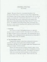
isolated pseudo-holomorphic triangles on the symmetric product are <strong>in</strong> 1-to-1 correspondence with<br />
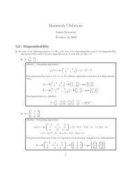
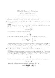
doma<strong>in</strong>s on the grid <strong>of</strong> certa<strong>in</strong> shapes, as shown <strong>in</strong> Figure 4.<br />
No such easy description is available for counts <strong>of</strong> pseudo-holomorphic m-gons on Sym n (G) with<br />
m ≥ 4. The trouble is that, unlike for m = 2 or 3, the counts for m ≥ 4 depend on the choice<br />
<strong>of</strong> a generic family J <strong>of</strong> almost complex structures on Sym n (G). Still, the counts are required to<br />
satisfy certa<strong>in</strong> constra<strong>in</strong>ts, com<strong>in</strong>g from positivity <strong>of</strong> <strong>in</strong>tersections and Gromov compactness. We<br />
def<strong>in</strong>e a formal complex structure on G to be any count <strong>of</strong> doma<strong>in</strong>s on the grid that satisfies these<br />
constra<strong>in</strong>ts.<br />
A formal complex structure is a purely comb<strong>in</strong>atorial object. Each such structure c gives rise<br />
to a complex C − (G,Λ,c), similar to (2), but where <strong>in</strong>stead <strong>of</strong> pseudo-holomorphic polygon counts<br />
we use the doma<strong>in</strong> counts prescribed by c. In particular, a family <strong>of</strong> almost complex structures J<br />
on the symmetric product produces a formal complex structure, whose correspond<strong>in</strong>g complex is<br />
exactly (2). There is a def<strong>in</strong>ition <strong>of</strong> homotopy between formal complex structures, and if two such<br />
structures are homotopic, they give rise to quasi-isomorphic complexes C − (G,Λ,c).<br />
We conjecture that any two formal complex structures on a grid diagram are homotopic. A<br />
weaker form <strong>of</strong> this conjecture, sufficient for our purposes, is proved <strong>in</strong> [MOT]. Instead <strong>of</strong> an<br />
ord<strong>in</strong>ary grid diagram G, we use its sparse double G#. This is obta<strong>in</strong>ed from G by <strong>in</strong>troduc<strong>in</strong>g n<br />
additional rows, columns, and O mark<strong>in</strong>gs, <strong>in</strong>terspersed between the previous rows and columns,
GRID DIAGRAMS IN HEEGAARD FLOER THEORY 11<br />
Figure 4. Snail doma<strong>in</strong>s. Darker shad<strong>in</strong>g corresponds to higher local multiplicities.<br />
The doma<strong>in</strong>s <strong>in</strong> each row (top or bottom) are part <strong>of</strong> an <strong>in</strong>f<strong>in</strong>ite sequence,<br />
correspond<strong>in</strong>g to <strong>in</strong>creas<strong>in</strong>g complexities. The larger circles represent certa<strong>in</strong> fixed<br />
po<strong>in</strong>ts on the grid, called destabilization po<strong>in</strong>ts. Each doma<strong>in</strong> corresponds to a<br />
pseudo-holomorphic triangle <strong>in</strong> the symmetric product <strong>of</strong> the grid.<br />
Figure 5. The sparse double <strong>of</strong> the grid diagram from Figure 2.<br />
as shown <strong>in</strong> Figure 5. The sparse double is not a grid diagram <strong>in</strong> the usual sense, because the new<br />
rows and columns have no X mark<strong>in</strong>gs. Nevertheless, it can still be viewed as a type <strong>of</strong> <strong>Heegaard</strong><br />
diagram for the l<strong>in</strong>k, and pseudo-holomorphic bigons and triangles correspond to empty rectangles<br />
and snail doma<strong>in</strong>s, just as before. One result <strong>of</strong> [MOT] is that on the sparse double, any two<br />
(sparse) formal complex structures are homotopic.<br />
With this <strong>in</strong> m<strong>in</strong>d, the desired algorithm for comput<strong>in</strong>g HF − is as follows: Choose any formal<br />
complex structure on G#, and then calculate the homology <strong>of</strong> C − (G,Λ,c). This homology is <strong>in</strong>dependent<br />
<strong>of</strong> c, so it agrees with the homology <strong>of</strong> the complex (2). By Theorem 5.2, this gives exactly<br />
HF − <strong>of</strong> surgery on the framed l<strong>in</strong>k. Similar algorithms can be constructed for comput<strong>in</strong>g HF +<br />
and ΦX,s. �
12 CIPRIAN MANOLESCU<br />
6. Open problems<br />
6.1. Develop more efficient algorithms. A weakness <strong>of</strong> the grid diagram approach is that the<br />
size <strong>of</strong> the comb<strong>in</strong>atorial knot <strong>Floer</strong> complex <strong>in</strong>creases super-exponentially (like n!) with respect to<br />
the size <strong>of</strong> the grid. Nevertheless, <strong>in</strong> practice, computer programs [BG, Dro08] can calculate knot<br />
<strong>Floer</strong> homology (for knots and l<strong>in</strong>ks <strong>in</strong> S 3 ) from <strong>diagrams</strong> <strong>of</strong> grid number up to 13. The algorithms<br />
become much less effective for 3-manifolds, and especially for 4-manifolds: this is because, for<br />
example, represent<strong>in</strong>g the K3 surface requires a grid <strong>of</strong> size at least 88.<br />
A related open problem is to decide whether the unknott<strong>in</strong>g problem can besolved <strong>in</strong> polynomial<br />
time.<br />
6.2. Comb<strong>in</strong>atorial pro<strong>of</strong>s. To completely set the <strong>theory</strong> <strong>in</strong> elementary terms, it rema<strong>in</strong>s to give<br />
purely comb<strong>in</strong>atorial pro<strong>of</strong>s that the <strong>Heegaard</strong> <strong>Floer</strong> <strong>in</strong>variants are <strong>in</strong>deed <strong>in</strong>variants <strong>of</strong> the underly<strong>in</strong>g<br />
object. For l<strong>in</strong>k <strong>Floer</strong> homology, this was achieved <strong>in</strong> [MOST07]. For � HF <strong>of</strong> 3-manifolds<br />
(def<strong>in</strong>ed from a class <strong>of</strong> <strong>diagrams</strong> called convenient, rather than from surgery formulas), a comb<strong>in</strong>atorial<br />
pro<strong>of</strong> <strong>of</strong> <strong>in</strong>variance appeared <strong>in</strong> [OSS]. The cases <strong>of</strong> the other versions <strong>of</strong> HF, and <strong>of</strong> the<br />
mixed <strong>in</strong>variants <strong>of</strong> 4-manifolds, rema<strong>in</strong> open.<br />
Also miss<strong>in</strong>g are comb<strong>in</strong>atorial pro<strong>of</strong>s for most <strong>of</strong> the topological properties <strong>of</strong> <strong>Heegaard</strong> <strong>Floer</strong><br />
<strong>theory</strong>. For example, it is not known how to prove comb<strong>in</strong>atorially that knot <strong>Floer</strong> homology<br />
detects the genus <strong>of</strong> a knot.<br />
6.3. Loose ends. In terms <strong>of</strong> show<strong>in</strong>g algorithmic computability, there are a few aspects <strong>of</strong> the<br />
<strong>theory</strong> that are not taken care <strong>of</strong> by Theorem 5.4:<br />
• Signs. Extend the comb<strong>in</strong>atorial descriptions to the <strong>in</strong>variants def<strong>in</strong>ed over Z (rather than<br />
over F = Z/2Z).<br />
• Cobordism maps. One can understand comb<strong>in</strong>atorially the maps on <strong>Heegaard</strong> <strong>Floer</strong> homology<br />
<strong>in</strong>duced by 2-handle cobordisms, and the mixed map for closed 4-manifolds, but not<br />
yet the maps <strong>in</strong>duced by a general cobordism between 3-manifolds (which may <strong>in</strong>clude 1and<br />
3-handles).<br />
• The uncompleted HF − and HF ∞ . Theorem5.4isaboutHF − ratherthanHF − . Fortorsion<br />
Sp<strong>in</strong> c structures, knowledge <strong>of</strong> HF − determ<strong>in</strong>es HF − . For nontorsion Sp<strong>in</strong> c structures,<br />
understand<strong>in</strong>g HF − is basically equivalent to understand<strong>in</strong>g HF − and HF ∞ ; the latter<br />
group has not yet been computed.<br />
6.4. Other open problems <strong>in</strong> <strong>Heegaard</strong> <strong>Floer</strong> <strong>theory</strong>. As mentioned <strong>in</strong> the <strong>in</strong>troduction, <strong>in</strong><br />
dimension 3, the <strong>Heegaard</strong>-<strong>Floer</strong> and Seiberg-Witten <strong>Floer</strong> homologies are known to be isomorphic.<br />
In dimension 4, it is still open to prove that the mixed Ozsváth-Szabó <strong>in</strong>variant <strong>of</strong> 4-manifolds is<br />
the same as the Seiberg-Witten <strong>in</strong>variant.<br />
Another important question is to understand the relationship <strong>of</strong> <strong>Heegaard</strong> <strong>Floer</strong> <strong>theory</strong> to Yang-<br />
Mills <strong>theory</strong>, and to the fundamental group <strong>of</strong> a 3-manifold.<br />
References<br />
[Bel10] Anna Beliakova, A simplification <strong>of</strong> comb<strong>in</strong>atorial l<strong>in</strong>k <strong>Floer</strong> homology, J. Knot Theory Ramifications 19<br />
(2010), no. 2, 125–144.<br />
[BG] JohnA.Baldw<strong>in</strong>andWilliam D.Gillam, Computations <strong>of</strong> <strong>Heegaard</strong>-<strong>Floer</strong> knot homology, Prepr<strong>in</strong>t,arXiv:<br />
math.GT/0610167.<br />
[BGH08] Kenneth L. Baker, J. Elisenda Grigsby, and Matthew Hedden, <strong>Grid</strong> <strong>diagrams</strong> for lens spaces and comb<strong>in</strong>atorial<br />
knot <strong>Floer</strong> homology, Int. Math. Res. Not. IMRN (2008), no. 10, Art. ID rnm024, 39.<br />
[BL] John A. Baldw<strong>in</strong> and Adam S. Lev<strong>in</strong>e, A comb<strong>in</strong>atorial spann<strong>in</strong>g tree model for knot <strong>Floer</strong> homology,<br />
Prepr<strong>in</strong>t (2011), arXiv:1105.5199.<br />
[Bru98] H. Brunn, Über verknotete Kurven, Verhandlungen des Internationalen Math. Kongresses (Zurich 1897)<br />
(1898), 256–259.
GRID DIAGRAMS IN HEEGAARD FLOER THEORY 13<br />
[CGHa] V<strong>in</strong>cent Col<strong>in</strong>, Paolo Ghigg<strong>in</strong>i, and Ko Honda, Embedded contact homology and open book decompositions,<br />
Prepr<strong>in</strong>t (2010), arXiv:1008.2734.<br />
[CGHb] , The equivalence <strong>of</strong> <strong>Heegaard</strong> <strong>Floer</strong> homology and embedded contact homology: from hat to plus,<br />
Prepr<strong>in</strong>t (2012), arXiv:1208.1526.<br />
[CGHc] , The equivalence <strong>of</strong> <strong>Heegaard</strong> <strong>Floer</strong> homology and embedded contact homology via open book decompositions<br />
I, Prepr<strong>in</strong>t (2012), arXiv:1208.1074.<br />
[CGHd] , The equivalence <strong>of</strong> <strong>Heegaard</strong> <strong>Floer</strong> homology and embedded contact homology via open book decompositions<br />
II, Prepr<strong>in</strong>t (2012), arXiv:1208.1077.<br />
[Don83] Simon K. Donaldson, An application <strong>of</strong> gauge <strong>theory</strong> to four-dimensional topology, J. Differential Geom.<br />
18 (1983), no. 2, 279–315.<br />
[Don90] , Polynomial <strong>in</strong>variants for smooth four-manifolds, Topology 29 (1990), no. 3, 257–315.<br />
[Dro08] Jean-Marie Droz, Effective computation <strong>of</strong> knot <strong>Floer</strong> homology, Acta Math. Vietnam. 33 (2008), no. 3,<br />
471–491.<br />
[Flo88] Andreas <strong>Floer</strong>, An <strong>in</strong>stanton-<strong>in</strong>variant for 3-manifolds, Comm. Math. Phys. 119 (1988), 215–240.<br />
[Frø96] Kim A. Frøyshov, The Seiberg-Witten equations and four-manifolds with boundary, Math. Res. Lett 3<br />
(1996), 373–390.<br />
[Gal08] Étienne Gallais, Sign ref<strong>in</strong>ement for comb<strong>in</strong>atorial l<strong>in</strong>k <strong>Floer</strong> homology, Algebr. Geom. Topol. 8 (2008),<br />
no. 3, 1581–1592.<br />
[Ghi08] Paolo Ghigg<strong>in</strong>i, Knot <strong>Floer</strong> homology detects genus-one fibred knots, Amer. J. Math. 130 (2008), no. 5,<br />
1151–1169.<br />
[Gre] Joshua E. Greene, The lens space realization problem, Prepr<strong>in</strong>t (2010), arXiv:1010.6257.<br />
[Kir78] Robion Kirby, A calculus for framed l<strong>in</strong>ks <strong>in</strong> S 3 , Invent. Math. 45 (1978), no. 1, 35–56.<br />
[KLTa] Ça˘gatay Kutluhan, Yi-Jen Lee, and Clifford H. Taubes, HF=HM I : <strong>Heegaard</strong> <strong>Floer</strong> homology and Seiberg–<br />
Witten <strong>Floer</strong> homology, Prepr<strong>in</strong>t (2010), arXiv:1007.1979.<br />
[KLTb] , HF=HM II : Reeb orbits and holomorphic curves for the ech/<strong>Heegaard</strong>-<strong>Floer</strong> correspondence,<br />
Prepr<strong>in</strong>t (2010), arXiv:1008.1595.<br />
[KLTc] , HF=HM III : Holomorphic curves and the differential for the ech/<strong>Heegaard</strong>-<strong>Floer</strong> correspondence,<br />
Prepr<strong>in</strong>t (2010), arXiv:1010.3456.<br />
[KLTd] , HF=HM IV : The Seiberg-Witten <strong>Floer</strong> homology and ech correspondence, Prepr<strong>in</strong>t (2010),<br />
arXiv:1107.2297.<br />
[KLTe] , HF=HM V : SeibergWitten <strong>Floer</strong> homology and handle additions, Prepr<strong>in</strong>t (2012),arXiv:1204.<br />
0115.<br />
[KM93] Peter B. Kronheimer and Tomasz S. Mrowka, Gauge <strong>theory</strong> for embedded surfaces. I, Topology 32 (1993),<br />
no. 4, 773–826.<br />
[KM07] , Monopoles and three-manifolds, New Mathematical Monographs, vol. 10, Cambridge University<br />
Press, Cambridge, 2007.<br />
[Lev08] Adam Simon Lev<strong>in</strong>e, Comput<strong>in</strong>g knot <strong>Floer</strong> homology <strong>in</strong> cyclic branched covers, Algebr. Geom. Topol. 8<br />
(2008), no. 2, 1163–1190.<br />
[Lic62] W. B. R. Lickorish, A representation <strong>of</strong> orientable comb<strong>in</strong>atorial 3-manifolds, Ann.<strong>of</strong> Math. (2) 76 (1962),<br />
531–540.<br />
[Lid] Tye Lidman, <strong>Heegaard</strong> <strong>Floer</strong> homology and triple cup products, Prepr<strong>in</strong>t (2010), arXiv:1011.4277.<br />
[Lip06] Robert Lipshitz, A cyl<strong>in</strong>drical reformulation <strong>of</strong> <strong>Heegaard</strong> <strong>Floer</strong> homology, Geom. Topol. 10 (2006), 955–<br />
1097.<br />
[LMW08] Robert Lipshitz, Ciprian Manolescu, and Jiajun Wang, Comb<strong>in</strong>atorial cobordism maps <strong>in</strong> hat <strong>Heegaard</strong><br />
<strong>Floer</strong> <strong>theory</strong>, Duke Math. J. 145 (2008), no. 2, 207–247.<br />
[LOT] Robert Lipshitz, Peter S. Ozsváth, and Dylan P. Thurston, Comput<strong>in</strong>g � HF by factor<strong>in</strong>g mapp<strong>in</strong>g classes,<br />
Prepr<strong>in</strong>t (2010), arXiv:1010.2550.<br />
[LS09] Paolo Lisca and András I. Stipsicz, On the existence <strong>of</strong> tight contact structures on Seifert fibered 3manifolds,<br />
Duke Math. J. 148 (2009), no. 2, 175–209.<br />
[Man03] Ciprian Manolescu, Seiberg-Witten-<strong>Floer</strong> stable homotopy type <strong>of</strong> three-manifolds with b1 = 0, Geom.<br />
Topol. 7 (2003), 889–932 (electronic).<br />
[MO] Ciprian Manolescu and Peter S. Ozsváth, <strong>Heegaard</strong> <strong>Floer</strong> homology and <strong>in</strong>teger surgeries on l<strong>in</strong>ks, Prepr<strong>in</strong>t<br />
(2010), arXiv:1011.1317.<br />
[MOS09] Ciprian Manolescu, Peter S. Ozsváth, and Sucharit Sarkar, A comb<strong>in</strong>atorial description <strong>of</strong> knot <strong>Floer</strong><br />
homology, Ann. <strong>of</strong> Math. (2) 169 (2009), no. 2, 633–660.<br />
[MOST07] Ciprian Manolescu, Peter S. Ozsváth, Zoltán Szabó, and Dylan P. Thurston, On comb<strong>in</strong>atorial l<strong>in</strong>k <strong>Floer</strong><br />
homology, Geom. Topol. 11 (2007), 2339–2412.<br />
[MOT] Ciprian Manolescu, Peter S. Ozsváth, and Dylan P. Thurston, <strong>Grid</strong> <strong>diagrams</strong> and <strong>Heegaard</strong> <strong>Floer</strong> <strong>in</strong>variants,<br />
Prepr<strong>in</strong>t (2009), arXiv:0910.0078.
14 CIPRIAN MANOLESCU<br />
[MW01] Matilde Marcolli and Bai-L<strong>in</strong>g Wang, Equivariant Seiberg-Witten <strong>Floer</strong> homology, Comm. Anal. Geom. 9<br />
(2001), no. 3, 451–639.<br />
[Ni07] Yi Ni, Knot <strong>Floer</strong> homology detects fibred knots, Invent. Math. 170 (2007), no. 3, 577–608.<br />
[Ni09] , <strong>Heegaard</strong> <strong>Floer</strong> homology and fibred 3-manifolds, Amer. J. Math. 131 (2009), no. 4, 1047–1063.<br />
[NOT08] Lenhard Ng, Peter Ozsváth, and Dylan Thurston, Transverse knots dist<strong>in</strong>guished by knot <strong>Floer</strong> homology,<br />
J. Symplectic Geom. 6 (2008), no. 4, 461–490.<br />
[OS03] Peter S. Ozsváth and Zoltán Szabó, Knot <strong>Floer</strong> homology and the four-ball genus, Geom. Topol. 7 (2003),<br />
615–639.<br />
[OS04a] , Holomorphic disks and genus bounds, Geom. Topol. 8 (2004), 311–334.<br />
[OS04b] , Holomorphic disks and knot <strong>in</strong>variants, Adv. Math. 186 (2004), no. 1, 58–116.<br />
[OS04c] , Holomorphic disks and three-manifold <strong>in</strong>variants: properties and applications, Ann. <strong>of</strong> Math. (2)<br />
159 (2004), no. 3, 1159–1245.<br />
[OS04d] , Holomorphic disks and topological <strong>in</strong>variants for closed three-manifolds, Ann. <strong>of</strong> Math. (2) 159<br />
(2004), no. 3, 1027–1158.<br />
[OS06] , Holomorphic triangles and <strong>in</strong>variants for smooth four-manifolds, Adv. Math. 202 (2006), no. 2,<br />
326–400.<br />
[OS08a] , Holomorphic disks, l<strong>in</strong>k <strong>in</strong>variants and the multi-variable Alexander polynomial, Algebr. Geom.<br />
Topol. 8 (2008), no. 2, 615–692.<br />
[OS08b] , Knot <strong>Floer</strong> homology and <strong>in</strong>teger surgeries, Algebr. Geom. Topol. 8 (2008), no. 1, 101–153.<br />
[OS09] , A cube <strong>of</strong> resolutions for knot <strong>Floer</strong> homology, J. Topol. 2 (2009), no. 4, 865–910.<br />
[OSS] Peter S. Ozsváth, András I. Stipsicz, and Zoltán Szabó, Comb<strong>in</strong>atorial <strong>Heegaard</strong> <strong>Floer</strong> homology and nice<br />
<strong>Heegaard</strong> <strong>diagrams</strong>, Prepr<strong>in</strong>t (2009), arXiv:0912.0830.<br />
[OSS11] , A comb<strong>in</strong>atorial description <strong>of</strong> the U 2 = 0 version <strong>of</strong> <strong>Heegaard</strong> <strong>Floer</strong> homology, Int. Math. Res.<br />
Not. IMRN (2011), no. 23, 5412–5448.<br />
[OST08] Peter S. Ozsváth, Zoltán Szabó, and Dylan Thurston, Legendrian knots, transverse knots and comb<strong>in</strong>atorial<br />
<strong>Floer</strong> homology, Geom. Topol. 12 (2008), no. 2, 941–980.<br />
[Per08] Timothy Perutz, Hamiltonian handleslides for <strong>Heegaard</strong> <strong>Floer</strong> homology, Proceed<strong>in</strong>gs <strong>of</strong> Gökova<br />
Geometry-Topology Conference 2007, Gökova Geometry/Topology Conference (GGT), Gökova, 2008,<br />
pp. 15–35.<br />
[Ras03] Jacob A. Rasmussen, <strong>Floer</strong> homology and knot complements, Ph.D. thesis, Harvard University, 2003,<br />
arXiv:math.GT/0306378.<br />
[Ras10] , Khovanov homology and the slice genus, Invent. Math. 182 (2010), no. 2, 419–447.<br />
[Sar] Sucharit Sarkar, <strong>Grid</strong> <strong>diagrams</strong> and the Ozsvath-Szabo tau-<strong>in</strong>variant, Prepr<strong>in</strong>t (2010), arXiv:1011.5265.<br />
[SW94a] Nathan Seiberg and Edward Witten, Electric-magnetic duality, monopole condensation, and conf<strong>in</strong>ement<br />
<strong>in</strong> N = 2 supersymmetric Yang-Mills <strong>theory</strong>, Nuclear Phys. B 426 (1994), no. 1, 19–52.<br />
[SW94b] , Monopoles, duality and chiral symmetry break<strong>in</strong>g <strong>in</strong> N = 2 supersymmetric QCD, Nuclear Phys.<br />
B 431 (1994), no. 3, 484–550.<br />
[SW10] Sucharit Sarkar and Jiajun Wang, An algorithm for comput<strong>in</strong>g some <strong>Heegaard</strong> <strong>Floer</strong> homologies, Ann. <strong>of</strong><br />
Math. (2) 171 (2010), no. 2, 1213–1236.<br />
[Wal60] Andrew H. Wallace, Modifications and cobound<strong>in</strong>g manifolds, Canad. J. Math. 12 (1960), 503–528.<br />
[Wit94] Edward Witten, Monopoles and four-manifolds, Math. Res. Lett. 1 (1994), 769–796.<br />
<strong>Department</strong> <strong>of</strong> Mathematics, <strong>UCLA</strong>, 520 Portola Plaza, Los Angeles, CA 90095, USA<br />
E-mail address: cm@math.ucla.edu