chapter 3 hydraulics of open channel flow

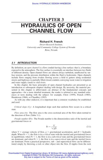
3.1 INTRODUCTION 

Source: HYDRAULIC DESIGN HANDBOOK 

CHAPTER 3 

HYDRAULICS OF OPEN 

CHANNEL FLOW 

Richard H. French 

Desert Research Institute, 

University and Community College System of Nevada 

Reno, Nevada 

By definition, an open channel is a flow conduit having a free surface: that is, a boundary 

exposed to the atmosphere. The free surface is essentially an interface between two fluids 

of different density. Open-channel flows are almost always turbulent, unaffected by surface 

tension, and the pressure distribution within the fluid is hydrostatic. Open channels 

include flows ranging from rivulets flowing across a field to gutters along residential 

streets and highways to partially filled closed conduits conveying waste water to irrigation 

and water supply canals to vital rivers. 

In this chapter, the basic principles of open channel hydraulics are presented as an 

introduction to subsequent chapters dealing with design. By necessity, the material presented 

in this chapter is abbreviated—an abstract of the fundamental concepts and 

approaches—for a more detailed treatment, the reader is referred to any standard references 

or texts dealing with the subject: for example, Chow (1959), French (1985), 

Henderson (1966), or Chaudhry (1993) 

As with any other endeavor, it is important that a common vocabulary be established 

and used: 

Critical slope (Sc ): A longitudinal slope such that uniform flow occurs in a critical 

state. 

Flow area (A): The flow area is the cross-sectional area of the flow taken normal to 

the direction of flow (Table 3.1). 

Froude number (Fr): The Froude number is the dimensionless ratio of the inertial and 

gravitational forces or 

Fr � � 

V 

� (3.1) 

�g�D� 

where V � average velocity of flow, g � gravitational acceleration, and D � hydraulic 

depth. When Fr � 1, the flow is in a critical state with the inertial and gravitational forces 

in equilibrium; when Fr � 1, the flow is in a subcritical state and the gravitational forces 

are dominant; and when Fr � 1, the flow is in a supercritical state and the inertial forces 

are dominant. From a practical perspective, sub – and supercritical flow can be differentiated 

simply by throwing a rock or other object into the flow. If ripples from the rock 

3.1 

Downloaded from Digital Engineering Library @ McGraw-Hill (www.digitalengineeringlibrary.com) 

Copyright © 2004 The McGraw-Hill Companies. All rights reserved. 

Any use is subject to the Terms of Use as given at the website.

TABLE 3.1 Channel Section Geometric Properties 

Channel Definition Area Wetted Perimeter Hydraulic Radius Top Width Hydraulic Depth 

A P R T D 

(1) (2) (3) (4) (5) (6) 

3.2 

by b � 2y 

by 

�� b y 

b � 2y 

Rectangle 

HYDRAULICS OF OPEN CHANNEL FLOW 

Trapezoid 

with 

equal side (b � zy)y b � 2y�1� �� z� 2� 

(b � zy) 

y 

� 

b � 2y�1� 

�� z� 2� 

� b � 2zy � ( b � zy) 

y 

� 

b � 2zy 

slopes 

by � 0.5y2 (z1 � z2) �� 

b � y(z1 � z2) � y ( �1� 

�� 

� �1� 

�� z� 2 z� 2� 1 

2�) 

Trapezoid 

with 

� b � y (z 1 + z 2 ) 

by � 0.5y2 (z1 � z 

��2) 

b � y(�1� �� z� 2� 1 � �1� �� z� 2 2�) 

unequal by � 0.5y 2 (z 1 � z 2 ) � b 

side slopes 

Triangle 

with equal zy2 2y�1� �� z� 2� 

zy 

� 

2�1� �� z� 2� 

� 2zy 0.5y 

side slopes 

Triangle 

with 0.5y2 (z1 � z2 ) y (�1� �� z� 2� 1 � �1� �� z� 2 0.5y 

2�) y (z1 � z2) 0.5y 

unequal 

side slopes 

2 ( z1 � z2 ) 

�� 

y (�1� �� z� 2� 1 � �1� �� z� 2 2�) 

2�y( � d� o�� y� )� � 1 

8 � ⎡ θ � sinθ 

⎢ �� ⎣ sin(0.5θ) 

⎤ ⎥ 

⎦ 

� 1 

8 �(θ � sinθ )do 2 0.5θdo 0.25 ⎛ ⎜1 � � 

⎝ 

sinθ 

⎞ 

� ⎟⎠ do θ 



Any use is subject to the Terms of Use as given at the website. 

CircularFigure T3.1-6

progress upstream of the point of impact, the flow is subcritical; however, if ripples from 

the rock do not progress upstream but are swept downstream, the flow is supercritical. 

Hydraulic depth (D). The hydraulic depth is the ratio of the flow area (A) to the top 

width (T) or D � A/T (Table 3.1). 

Hydraulic radius (R). The hydraulic radius is the ratio of the flow area (A) to the wetted 

perimeter (P) or R � A/P (Table 3.1). 

Kinetic energy correction factor (α). Since no real open-channel flow is one-dimensional, 

the true kinetic energy at a cross section is not necessarily equal to the spatially 

averaged energy. To account for this, the kinetic energy correction factor is introduced, or 

α�γ� V3 

�� 2g 

A �∫∫γ� v3 

� dA 

2g 

and solving for α, 

α � � ∫∫v 

V 

3dA 

3� 

(3.2) 

A 

When the flow is uniform, α � 1 and values α of for various situations are summarized 

in Table 3.2. 

Momentum correction coefficient (β): Analogous to the kinetic energy correction factor, 

the momentum correction factor is given by 

βρQV � ∫∫ρv 2 dA 

Hydraulics of Open–Channel Flow 3.3 

β � � ∫∫v 

V 

2dA 

2� 

(3.3) 

A 

When the flow is uniform, β � 1 and values of β for various situations are summarized in 

Table 3.2 

Prismatic channel. A prismatic channel has both a constant cross-sectional shape and 

bottom slope (So ). Channels not meeting these criteria are termed nonprismatic. 

Specific energy (E). The specific energy of an open-channel flow is 

V2 

E � y � α�� (3.4) 

2g 

where y � depth of flow and the units of specific energy are length in meters or feet. 

TABLE 3.2 Typical Values of α and β for Various Situations 

Situation Value of α Value of β 

Min. Avg. Max. Min. Avg. Max. 

Regular channels, flumes, 1.10 1.15 1.20 1.03 1.05 1.07 

spillways 

Natural streams and torrents 1.15 1.30 1.50 1.05 1.10 1.17 

Rivers under ice cover 1.20 1.50 2.00 1.07 1.17 1.33 

River valleys, overflooded 1.50 1.75 2.00 1.17 1.25 1.33 

Source: After Chow (1959). 





3.4 Chapter Three 

Specific momentum (M). By definition, the specific momentum of an open-channel 

flow is 

Q2 

M � �� + z 

gA 

�A (3.5) 

Stage: The stage of a flow is the elevation of the water surface relative to a datum. If 

the lowest point of a channel section is taken as the datum, then the stage and depth of 

flow (y) are equal if the longitudinal slope (So ) is not steep or cos (θ) ≈ 1, where θ is the 

longitudinal slope angle. If θ � 10 o or So � 0.18, where So is the longitudinal slope of the 

channel, then the slope of the channel can be assumed to be small. 

Steady. The depth (y) and velocity of flow (v) at a location do not vary with time; that 

is, (∂y/∂t � 0) and (∂v/∂t � 0). In unsteady flow, the depth and velocity of flow at a location 

vary with time: that is, (∂y/∂t ≠ 0) and (∂v/∂t ≠ 0). 

Top width (T). The top width of a channel is the width of the channel section at the 

water surface (Table 3.1). 

Uniform flow. The depth (y). flow area (A), and velocity (V) at every cross section are 

constant, and the energy grade line (Sf ), water surface, and channel bottom slopes (So ) are 

all parallel. 

Superelevation (∆y). The rise in the elevation of the water surface at the outer channel 

boundary above the mean depth of flow in an equivalent straight channel, because of centrifugal 

force in a curving channel. 

Wetted perimeter (P). The wetted perimeter is the length of the line that is the interface 

between the fluid and the channel boundary (Table 3.1). 

3.2 ENERGY PRINCIPLE 

3.2.1 Definition of Specific Energy 


Central to any treatment of open-channel flow is that of conservation of energy. The 

total energy of a particle of water traveling on a streamline is given by the Bernoulli 

equation or 

H � z � � p 

γ � � α � V2 

� 

2g 

where H � total energy, z � elevation of the streamline above a datum, p � pressure, γ 

� fluid specific weight, (p/γ) � pressure head, V 2 /2g � velocity head, and g � acceleration 

of gravity. H defines the elevation of the energy grade line, and the sum [z � (p/γ)] 

defines the elevation of the hydraulic grade line. In most uniform and gradually varied 

flows, the pressure distribution is hydrostatic (divergence and curvature of the streamlines 

is negligible) and the sum [z + (p/γ)] is constant and equal to the depth of flow y if the 

datum is taken at the bottom of the channel. The specific energy of an open-channel flow 

relative to the channel bottom is 

V2 

Q2 

E � y � α�� y � α 

2g 

�� 2gA2 

(3.6) 




where the average velocity of flow is given by 

V � � Q 

� (3.7) 

A 

where Q � flow rate and A � flow area. 

The assumption inherent in Eq. (3.6) is that the slope of the channel is small, or cos(θ) 

� 1. If θ � 10° or So � 0.18, where So is the longitudinal slope of the channel, Eq. (3.6) 

is valid. If θ is not small, then the pressure distribution is not hydrostatic since the vertical 

depth of flow is different from the depth measured perpendicular to the bed of the 

channel. 

3.2.2 Critical Depth 


If y in Eq. (3.6) is plotted as a function of E for a specified flow rate Q, a curve with two 

branches results. One branch represents negative values of both E and y and has no physical 

meaning; but the other branch has meaning (Fig. 3.1). With regard to Fig. 3.1, the following 

observations are pertinent: 1) the portion designated AB approaches the line y � E 

asymptotically, 2) the portion AC approaches the E axis asymptotically, 3) the curve has 

a minimum at point A, and 4) there are two possible depths of flow—the alternate 

depths—for all points on the E axis to the right of point A. The location of point A, the 

minimum depth of flow for a specified flow rate, can be found by taking the first derivative 

of Eq. (3.6) and setting the result equal to zero, or 

� dE 

Q2 

� � 1 � �� dy 

gA3 

� dA 

� � 0 (3.8) 

dy 

It can be shown that dA � (T � dy) or (dA/dy � T) (French, 1985). Substituting this 

result, using the definition of hydraulic depth and rearranging, Eq. (3.8) becomes 

y 

y c 


Specific Momentum 

FIGURE 3.1 Specific energy and momentum as a function of depth when the channel geometry 

and flow rate are specified. 





or 

and 

Q2 

1 � �� gA3 

� dA 

Q2 

T V2 

� � 1 � �� dy 

gA2 

�� 1 � �g � � 0 

A D 

V2 

�� 

2g 

D 

� (3.9) 

2 

� 

V 

� � Fr � 1 (3.10) 

�g�D� 

which is the definition of critical flow. Therefore, minimum specific energy occurs at the 

critical hydraulic depth and is the minimum energy required to pass the flow Q. With this 

information, the portion of the curve AC in Fig. 3.1 is interpreted as representing supercritical 

flows, where as AB represents subcritical flows. 

With regard to Fig. 3.1 and Eq. (3.6), the following observations are pertinent. First, 

for channels with a steep slope and α ≠ 1, it can be shown that 

V 

�� 

Fr � (3.11) 

�� g � D � c 

�α o � s( 

� θ � ) �� 

Second, E – y curves for flow rates greater than Q lie to the right of the plotted curve, 

and curves for flow rates less than Q lie to the left of the plotted curve. Third, in a rectangular 

channel of width b, y � D and the flow per unit width is given by 

q � � Q 

� (3.12) 

b 

and 

and 


V � � q 

� 

y 

Then, where the subscript c indicates variable values at the critical point, 

(3.13) 

yc � �� q2 

�� g 

1/3 

(3.14) 

� V 

2 

c 

� � � 

2g 

yc 

� 

2 

(3.15) 

yc � � 2 

3 � Ec (3.16) 

In nonrectangular channels when the dimensions of the channel and flow rate are specified, 

critical depth is calculated either by the trial and error solution of Eqs. (3.8), (3.9), 

and (3.10) or by use of the semiempirical equations in Table 3.3. 

3.2.3 Variation of Depth with Distance 

At any cross section, the total energy is 

V2 

H � �� y � z (3.17) 

2g 





TABLE 3.3 Semiempirical Equations for the Estimation of y c 

Channel Definition Equation for y c 

(1) in terms of 

Ψ � α Q 2 /g 

(2) 

Rectangle 

Figure T3.1-1 

⎛ 

⎜ 

⎝ � Ψ 

� 

b2 

⎞ 0.33 

⎟ 

⎠ 

TrapezoidFig 

ure T-3.1-2 0.81 ⎛ Ψ 

⎜ � 

⎝ z0.75 b1.25 � ⎞ ⎟ 

⎠ 

TriangleFigure T3.1-4 

CircleFigure T3.1-6 

Source: From Straub (1982). 

⎛ 

⎜ 

⎝ �2 

Ψ 

� 

z2 

⎞0.20 ⎟ 

⎠ 


⎛ 

⎜ 

⎝ � 1.01 

� 

d 0.26 

o 

⎞ ⎟ Ψ 

⎠ 0.25 

0.27 

� 

b 

� 

30z 

� 

where y � depth of flow, z � elevation of the channel bottom above a datum, and it is 

assumed that and cos(θ) are both equal to 1. Differentiating Eq. (3.17) with respect to longitudinal 

distance, 

� dH 

� � � � 

dx 

dy 

dz 

� � �� (3.18) 

dx 

dx 

where � dH 

dz 

d 

� 

x 

� the change of energy with longitudinal distance (Sf ), �� the channel bottom 

slope (S 

dx 

o ), and, for a specified flow rate, 

Q2 

� �� 

gA3 

dA 

� � 

dy 

dy 

� �� 

dx 

Q2T3 

� � 

gA 

dy 

� ��(Fr) 

dx 

2 � d 

d� y 

� 

dx 

� d� 

V2 

�� 2g 

� 

dx 

� V2 

�� 2g 

� 

dx 

Substituting these results in Eq. (3.18) and rearranging, 

� dy 

So � S 

� � � 

dx 

1 � Fr2 

f 

� 

(3.19) 

which describes the variation of the depth of flow with longitudinal distance in a channel 

of arbitrary shape. 





3.2.4 Compound Section Channels 

In channels of compound section (Fig. 3.2), the specific energy correction factor α is not 

equal to 1 and can be estimated by 

A2 

i 

� 

α � (3.20) 

� K3 

� 

where K i and A i as follows the conveyance and area of the ith channel subsection, respectively, 

K and A are conveyance are as follows: 

and 

N 

K �� Ki i � 1 

N 

A �� Ai i � 1 

N � number of subsections, and conveyance (K) is defined by Eq. (3.48) in Sec. 3.4. 

Equation (3.20) is based on two assumptions: (1) the channel can be divided into subsections 

by appropriately placed vertical lines (Fig. 3.2) that are lines of zero shear and do 

not contribute to the wetted perimeter of the subsection, and (2) the contribution of the 

nonuniformity of the velocity within each subsection is negligible in comparison with the 

variation in the average velocity among the subsections. 

3.3 MOMENTUM 


FIGURE 3.2 Channel with a compound section. 

N 

� 

i � 1��K 3 

i �� 

3.3.1 Definition of Specific Momentum 

The one-dimensional momentum equation in an open channel of arbitrary shape and a 

control volume located between Sections 1 and 2 is 




A 2

γ 

γz �1A1 � γ �2 z A2 � Pf � �� Q (V2 � V1 ) (3.21) 

g 

where γ � specific weight of water, A i � flow area at sections 1 and 2; V i � average velocity 

of flow at sections 1 and 2, P f � horizontal component of unknown force acting 

between Sections 1 and 2 and z w i � distances to the centroids of the flow areas 1 and 2 from 

the free surface. Substitution of the flow rate divided by the area for the velocities and 

rearrangement of Eq. (3.21) yields 

or 


� Pf 

� � 

γ �� Q2 

gA 

� � �1 z A1� � �� Q2 

gA 

� � �2 z A2� 1 

� Pf 

� � M1 � M2 (3.22) 

γ 

where 

Q2 

Mi � �� i z Ai (3.23) 

gAi 

and M is known as the specific momentum or force function. In Fig. 3.1, specific momentum 

is plotted with specific energy for a specified flow rate and channel section as a function 

of the depth of flow. Note that the point of minimum specific momentum corresponds 

to the critical depth of the flow. 

The classic application of Eq. (3.22) occurs when Pf � 0 and the application of the resulting 

equation to the estimation of the sequent depths of a hydraulic jump. Hydraulic jumps 

result when there is a conflict between the upstream and downstream controls that influence 

the same reach of channel. For example, if the upstream control causes supercritical flow 

while the downstream control dictates subcritical flow, there is a contradiction that can be 

resolved only if there is some means to pass the flow from one flow regime to the other. When 

hydraulic structures, such as weirs, chute blocks, dentated or solid sills, baffle piers, and the 

like, are used to force or control a hydraulic jump, Pf in Eq. (3.22) is not equal to zero. Finally, 

the hydraulic jump occurs at the point where Eq. (3.22) is satisfied (French, 1985). 

3.3.2 Hydraulic Jumps in Rectangular Channels 

In the case of a rectangular channel of width b and Pf � 0, it can be shown (French, 

1985) that 

� y2 

� � �0�.5� [�1� �� 8�(F�r�) 1 

y1 

2� � 1] (3.24) 

or 

y1 2 

y1 �� 0.5 [�1� �� 8�(F�r�) 2 

y2 

2 

�� 2(Fr2 ) 

y 

2 � 4(Fr2 ) 4 � 16(Fr2 ) 6 � ... 


2 

� ��1�] (3.25) 

Equations (3.24) and (3.25) each contain three independent variables, and two must be 

known before the third can be found. It must be emphasized that the downstream depth of 

flow (y 2 ) is not the result of upstream conditions but is the result of a downstream control—that 

is, if the downstream control produces the depth y 2 then a hydraulic jump will 

form. The second form of Eq. (3.25) should be used when (Fr 2 ) 2 � 0.05 (French, 1985). 





3.3.3 Hydraulic Jumps in Nonrectangular Channels 

In analyzing the occurrence of hydraulic jumps in nonrectangular but prismatic channels, we 

see that no equations are analogous to Eqs. (3.24) and (3.25). In such cases, Eq. (3.22) could 

be solved by trial and error or by use of semiempirical equations. For example, in circular sections, 

Straub (1978) noted that the upstream Froude number (Fr1 ) can be approximated by 

yc 

1.93 

(3.26) 

Fr1 � ⎛ ⎜�� ⎝y1 ⎞ ⎟ 

⎠ 

and the sequent depth can be approximated by 

y2 

c 

Fr1 � 1.7y2 � �� (3.27 

y1 

Fr1 � 1.7y2 � � y1. 

8 

c 

� 0. 

73 

(3.28) 

y1 

For horizontal triangular and parabolic prismatic channel sections, Silvester (1964, 

1965) presented the following equations. 

For triangular channels: 

⎛ 

⎜ 

⎝ �y 

2 

� 

y1 

⎞2.5 ⎟ � 1 � 1.5 (Fr1 ) 

⎠ 

2 ⎡ ⎢ 1 � 

⎣ ⎛ ⎜� ⎝ y1 

� 

y2 

⎞2⎤⎥⎦ ⎟ 

⎠ 

(3.29) 

For parabolic channels with the perimeter defined by y � aT 2 /2, where a is a 

coefficient: 

� y 

� 

2 

y1 


⎛ 

⎜ 

⎝ �y 

2 

� 

y1 

⎞2.5 ⎟ � 1 � 1.67 (Fr1 ) 

⎠ 

2 ⎡ ⎢ 1 � 

⎣ ⎛ ⎜� ⎝ y1 

� 

y2 

⎞1.5 ⎤⎥⎦ 

⎟ 

⎠ 

FIGURE 3.3 Analytic curves for estimating sequent depths in a trapezoidal channel 

(From Silvester, 1964) 

(3.30) 




In the case of trapezoidal channels, Silvester (1964) presented a method for graphical 

solution in terms of the parameter 

b 

k � �� (3.31) 

zy1 

In Fig. 3.3, the ratio of (y2 /y1 ) is plotted as a function of Fr1 and k. 

3.4 UNIFORM FLOW 

3.4.1 Manning and Chezy Equations 


For computational purposes, the average velocity of a uniform flow can be estimated by 

any one of a number of semiempirical equations that have the general form 

V � CR x S y 

(3.32) 

where C � a resistance coefficient, R � hydraulic radius, S � channel longitudinal slope, 

and x and y are exponents. At some point in the period 1768–1775 (Levi, 1995), Antoine 

Chezy, designing an improvement for the water system in Paris, France, derived an equation 

relating the uniform velocity of flow to the hydraulic radius and the longitudinal slope 

of the channel, or 

V � C �R�S� (3.33) 

where C is the Chezy resistance coefficient. It can be easily shown that Eq (3.33) is similar 

in form to the Darcy pipe flow equation. In 1889, Robert Manning, a professor at the 

Royal College of Dublin (Levi, 1995) proposed what has become known as Manning’s 

equation, or 

V = � φ 

n � R2/3�S� (3.34) 

where n is Manning’s resistance coefficient and φ � 1 if SI units are used and φ � 1.49 

if English units are used. The relationship among C, n, and the Darcy-Weisbach friction 

factor (f) is 

C � � φ 

n � R1/6 �� 8 

�f g �� 

(3.35) 

At this point, it is pertinent to observe that n is a function of not only boundary roughness 

and the Reynolds number but also the hydraulic radius, an observation that was made 

by Professor Manning (Levi, 1995). 

3.4.2 Estimation of Manning’s Resistance Coefficient 

Hydraulics of Open-Channel Flow 3.11 

Of the two equations for estimating the velocity of a uniform flow, Manning’s equation is 

the more popular one. A number of approaches to estimating the value of n for a channel 

are discussed in French (1985) and in other standard references, such as Barnes (1967), 

Urquhart (1975), and Arcement and Schneider (1989). Appendix 3.A lists typical values 

of n for many types of common channel linings. 






In an unvegetated alluvial channel, the total roughness consists of two parts: grain or 

skin roughness resulting from the size of the sediment particles and form roughness 

because of the existence of bed forms. The total coefficient n can be expressed as 

n � n’ � n” (3.36) 

where n’ � portion of Manning’s coefficient caused by grain roughness and n” � portion 

of Manning’s coefficient caused by form roughness. The value of n’ is proportional to the 

diameter of the sediment particles to the sixth power. For example, Lane and Carlson 

(1953) from field experiments in canals paved with cobbles with d 75 in inches, developed 

1/6 

n’ � 0.026d75 (3.37) 

and Meyer-Peter and Muller (1948) for mixtures of bed material with a significant proportion 

of coarse-grained sizes with d90 in meters developed 

1/6 

n’ � 0.038d90 (3.38) 

In both equations, dxx is the sediment size such that xx percent of the material is smaller 

by weight. 

Although there is no reliable method of estimating n”, an example of the variation of 

f for the 0.19 mm sand data collected by Guy et al. (1966) is shown in Fig. 3.4. The n values 

commonly found for different bed forms are summarized in Table 3.4. The inability 

to estimate or determine the variation of form roughness poses a major problem in the 

study of alluvial hydraulics (Yang, 1996). 

Use of Manning’s equation to estimate the velocity of flow in channels where the primary 

component of resistance is from drag rather than bed roughness has been questioned 

(Fischenich, 1996). However, the use of Manning’s equation has persisted among engineers 

because of its familiarity and the lack of a practical alternative. Jarrett (1984) recognized that 

FIGURE 3.4 Variation of the Darcy-Weisbach friction factor as a function of unit stream power. 





guidelines for estimating resistance coefficients for high-gradient streams with stable beds 

composed of large cobbles and boulders and minimally vegetated banks (So � 0.002) were 

based on limited data. Jarrett (1984) examined 21 high-gradient streams in the Rocky 

Mountains and developed the following empirical equation relating n to So and R (in feet): 

n � � 0.39S 

0.38 

0 

� (3.39) 

R0.16 

Jarrett (1984) stated the following limitations on the use of Eq. (3.39): First, the equation 

is applicable to natural main channels with stable bed and bank materials (gravels, 

cobbles, boulders) with no backwater. Second, the equation can be used for 0.002 � So � 

0.04 and 0.15 � R � 2.1 m (0.5 � R � 7.0 ft). Results of the regression analysis indicated 

that for R � 2.1 m ( 7.0 ft), n did vary significantly with depth; therefore, as long as 

the bed and bank material remain stable, extrapolation to larger flows should not result in 

significant error. Third, the hydraulic radius does not include the wetted perimeter of the 

bed particles. Fourth, the streams used in the analysis had relatively small amounts of suspended 

sediment. 

Vegetated channels present unique challenges from the viewpoint of estimating roughness. 

In grass-lined channels, the traditional approach assumed that n was a function of 

vegetal retardance and VR (Coyle, 1975). However, there are approaches more firmly 

based on the principles of fluid mechanics and the mechanics of materials (Kouwen, 1988; 

Kouwen and Li, 1980.) Data also exist that suggest that in such channels flow duration is 

not a factor as long as the vegetal elements are not destroyed or removed. Further, inundation 

times, and/or hydraulic stresses, or both that are sufficient to damage vegetation 

have been found, as might be expected, to reduce the resistance to flow (Temple, 1991). 

Petryk and Bosmajian (1975) presented a relation for Manning’s n in vegetated channels 

based on a balance of the drag and gravitational forces, or 

n ��R2/3 ⎡ ⎢ � 

⎣ Cd ( Veg) 

d 

� 

2g 

⎤1/2 ⎥ 

⎦ 

(3.40) 

where C d a coefficient accounting for the drag characteristics of the vegetation and (Veg) d 

the vegetation density. Flippin-Dudley (1997) has developed a rapid and objective 

procedure using a horizontal point frame to measure (Veg) d . Equation (3.40) is limited 

because there is limited information regarding C d for vegetation (Flippin-Dudley 

et al., 1997). 

3.4.3 Equivalent Roughness Parameter k 

In some cases, an equivalent roughness parameter k is used to estimate n. Equivalent 

roughness, sometimes called “roughness height,” is a measure of the linear dimension 

of roughness elements but is not necessarily equal to the actual or even the average height 

of these elements. The advantage of using k instead of Manning’s n is that k accounts for 

changes in the friction factor due to stage, whereas the Manning’s n does not. The relationship 

between n and k for hydraulically rough channels is 

�R1/6 ⎛ 

�log10⎜ 12.2 �R 

⎝ k � ⎞ ⎟ 

⎠ 

where Γ � 32.6 for English units and 18.0 for SI units. 


n � �� 

(3.41) 






TABLE 3.4 Equivalent Roughness Values of Various Bed Materials 

Material k k 

(ft) (m) 

(1) (2) (3) 

Brass, copper, lead, glass 0.0001–0.0030 0.00003048–0.0009 

Wrought iron, steel 0.0002–0.0080 0.0001–0.0024 

Asphalted cast iron 0.0004–0.0070 0.0001–0.0021 

Galvanized iron 0.0005–0.0150 0.0002–0.0046 

Cast iron 0.0008–0.0180 0.0002–0.0055 

Wood stave 0.0006–0.0030 0.0002–0.0009 

Cement 0.0013–0.0040 0.0004–0.0012 

Concrete 0.0015–0.0100 0.0005–0.0030 

Untreated gunite 0.01–0.033 0.0030–0.0101 

Drain tile 0.0020–0.0100 0.0006–0.0030 

Riveted steel 0.0030–0.0300 0.0009–0.0091 

Rubble masonry 0.02 0.0061 

Straight, uniform earth 0.01 0.0030 

channels 

Natural streambed 0.1000-3.0000 0.0305-0.9144 

Sources: From Ackers C (1958), Chow (1959), and Zegzhda (1938). 

With regard to Eq. (3.41), it is pertinent to observe that as R increases (equivalent to 

an increase in the depth of flow), n increases. Approximate values of k for selected 

materials are summarized in Table 3.4. For sand-bed channels, the following sediment 

sizes have been suggested by various investigators for estimating the value of k: k � d 65 

(Einstein, 1950), k � d 90 (Meyer-Peter and Muller, 1948), and k � d 85 (Simons and 

Richardson, 1966). 

3.4.4 Resistance in Compound Channels 

In many designed channels and most natural channels, roughness varies along the perimeter 

of the channel, and it is necessary to estimate an equivalent value of n for the entire 

perimeter. In such cases, the channel is divided into N parts, each with an associated wetted 

perimeter (P i ), hydraulic radius (R i ), and roughness coefficient (n i ), and the equivalent 

roughness coefficient (n e ) is estimated by one of the following methods. Note that the wetted 

perimeter does not include the imaginary boundaries between the subsections. 

1. Horton (1933) and Einstein and Banks (1950) developed methods of estimating n e 

assuming that the average velocity in each of the subdivisions is the same as the 

average velocity of the total section. Then 

�� 

N 

� i � 1 

ne �� P 

�P 3/2 

ini � 

�2/3 

(3.42) 




2. Assuming that the total force resisting motion is equal to the sum of the subsection 

resisting forces, 

�1/2 

(3.43) 

3. Assuming that the total discharge of the section is equal to the sum of the subsection 

discharges, 

PR 

ne � (3.44) 

5/3 

�� 

N 

� PiRi 5/3 

� 

4. Weighting of resistance by area (Cox, 1973), 

5. The Colebatch method (Cox, 1973). 

� 

i � 1 

niAi i � 1 

ne � � 

A 

(3.45) 

N 

�� 

�i�1 

ne � A 

3.4.5 Solution of Manning’s Equation 

�2/3 

(3.46) 

The uniform flow rate is the product of the velocity of flow and the flow area, or 

Q � VA � � � 

n � AR2/3�S� (3.47) 

In Eq. (3.47), AR2/3 is termed the section factor and, by definition, the conveyance of the 

channel is 

K � � � 

n � AR2/3 (3.48) 

Before the advent of computers, the solution of Eq. (3.34) or Eq. (3.47) to estimate the 

depth of flow for specified values of V (or Q), n, and S was accomplished in one of two 

ways: by trial and error or by the use of a graph of AR2/3 versus y. In the age of the 

desktop computer, software is used to solve the equations of uniform flow. Trial and error 

and graphical approaches to the solution of the uniform flow equations can be found in 

any standard reference or text (e.g., French, 1985). 

3.4.6 Special Cases of Uniform Flow 


�� 

N 

� i � 1 

ne � P 

N 

� 

(P i n i 2) 

A i n i 3/2 

3.4.6.1 Normal and critical slopes. If Q, n, and y N (normal depth of flow) and the channel 

section are defined, then Eq. (3.47) can be solved for the slope that allows the flow to 

occur as specified; by definition, this is a normal slope. If the slope is varied while the discharge 

and roughness are held constant, then a value of the slope such that normal flow 

n i 






occurs in a critical state can be found: that is, a slope such that normal flow occurs with 

Fr � 1. The slope obtained is the critical slope, but it also is a normal slope. The smallest 

critical slope, for a specified channel shape, roughness, and discharge is termed the limiting 

critical slope. The critical slope for a given normal depth is 

gn2D 

Sc � � 

�2RN 

4/ 

N 

� (3.49) 

3 

where the subscript N indicates the normal depth value of a variable and, for a wide channel, 

gn2 

Sc � �� 2y 

1/3 

c 

(3.50) 

3.4.6.2 Sheetflow. A special but noteworthy uniform flow condition is that of sheetflow. 

From the viewpoint of hydraulic engineering, a necessary condition for sheetflow is that 

the flow width must be sufficiently wide so that the hydraulic radius approaches the depth 

of flow. With this stipulation, the Manning’s equation, Eq. (3.48), for a rectangular channel 

becomes 

Q � � � 

n � TyN 5/3 �S� (3.51) 

where T � sheetflow width and yN � normal depth of flow. Then, for a specified flow rate 

and sheetflow width, Eq. (3.51) can be solved for the depth of flow, or 

nQ 

yN � ⎛ ⎜ � 

⎝ �T �S� 

�⎞ 3/5 

⎟ 

⎠ 

(3.52) 

The condition that the value of the hydraulic radius approaches the depth of flow is not 

a sufficient condition. That is, this condition specifies no limit on the depth of flow, and 

there is general agreement that sheetflow has a shallow depth of flow. Appendix 3.A summarizes 

Manning’s n values for overland and sheetflow. 

3.4.6.3 Superelevation. When a body of water moves along a curved path at constant 

velocity, it is acted for a force directed toward the center of the curvature of the path. 

When the radius of the curve is much larger than the top width of the water surface, it can 

be shown that the rise in the water surface at the outer channel boundary above the mean 

depth of flow in a straight channel (or superelevation) is 

∆y � � V2T 

� (3.53) 

2gr 

where r � the radius of the curve (Linsley and Franzini, 1979). It is pertinent to note that 

if the effects of the velocity distribution and variations in curvature across the channel are 

considered, the superelevation may be as much as 20 percent more than that estimated by 

Eq. (3.53) (Linsley and Franzini, 1979). Additional information regarding superelevation 

is available in Nagami et al., (1982) and U.S. Army Corps of Engineers (USACE, 1970). 

3.5 GRADUALLY AND SPATIALLY VARIED FLOW 

3.5.1 Introduction 


The gradual variation in the depth of flow with longitudinal distance in an open channel 

is given by Eq. (3.19), or 





� dy 

So � Sf 

� � �� dx 

1 � Fr2 

and two cases warrant discussion. In the first case, because the distance over which the 

change in depth is short it is appropriate to assume that boundary friction losses are small, 

or Sf � 0. When this is the case, important design questions involve abrupt steps in the 

bottom of the channel (Fig. 3.5) and rapid expansions or contractions of the channel 

(Fig. 3.6). The second case occurs when Sf ≠ 0. 

3.5.2 Gradually Varied Flow with S f � 0 


When Sf � 0 and the channel is rectangular in shape and has a constant width, Eq. (3.19) 

reduces to 

(1 � Fr2 )� dy 

dz 

� � �� 0 (3.54) 

dx 

dx 

and the following observations are pertinent (the observations also apply to channels of 

arbitrary shape): 

1. If dz/dx � 0 (upward step) and Fr � 1, then dy/dx must be less than zero—depth 

of flow decreases as x increases. 

2. If dz/dx � 0 (upward step) and Fr � 1, then dy/dx must be greater than zero—depth 

of flow increases as x increases. 

FIGURE 3.5 Definition of variables for gradually varied flow over positive and negative 

steps. 






FIGURE 3.6 Definition of variables for gradually varied flow through contracting 

and expanding channel sections. 

3. If dz/dx � 0 (downward step) and Fr � 1, then dy/dx must be greater than zero— 

depth of flow increases as x increases. 

4. If dz/dx � 0 (downward step) and Fr � 1, then dy/dx must be less than zero—depth 


In the case of a channel of constant width with a positive or negative step, the relation 

between the specific energy upstream of the step and the specific energy downstream of 

the step is 

E1 =E2 + ∆z (3.55) 

In the case dz/dx � 0, if the channel is rectangular in shape but the width of the channel 

changes, it can be shown (French, 1985) that the governing equation is 

(1 � Fr2 )� dy 

� � Fr 

dx 

2 y dT 

�� 0 (3.56) 

b dx 

The following observations also apply to channels of arbitrary shape: 

1. If db/dx � 0 (width increases) and Fr � 1, then dy/dx must be greater than 

zero–depth of flow increases as x increases. 

2. If db/dx � 0 (width increases) and Fr � 1, then dy/dx must be less than zero—depth 





3. If db/dx � 0 (width decreases) and Fr � 1, then dy/dx must be less than zero— 

depth of flow decreases as x increases. 

4. If db/dx � 0 (width decreases) and Fr � 1, then dy/dx must be greater than zero— 

depth of flow increases as x increases. 

In this case, the relation between the specific energy upstream of the contraction 

(expansion) and the specific energy downstream of the step contraction (expansion) is 

E1 � E2 (3.57) 

It is pertinent to note that in the case of supercritical flow, channel expansions and contractions 

may result in the formation of waves. 

Additional information regarding steps, expansions, and contractions can be found in any 

standard reference or text on open-channel hydraulics (e.g., French, 1985). 

3.5.3 Gradually Varied Flow with S f � 0 

In the case where S f cannot be neglected, the water surface profile must estimated. For a 

channel of arbitrary shape, Eq. (3.19) becomes 

� dy 

n 

� � �So� (3.60) 

dx 

2 Q2 P4/3 � 

1�� Q 

So � Sf � 

2 T 

1�� 

gA3� 

Q2T 

� 

gA3 

For a specified value of Q, Fr and S f are functions of the depth of flow y. For illustrative 

purposes, assume a wide channel; in such a channel, Fr and S f will vary in much the 

same way with y since P � T and both S f and Fr have a strong inverse dependence on the 

flow area. In addition, as y increases, both S f and Fr decrease. By definition, S f � S o when 

y � y N . Given the foregoing, the following set of inequalities must apply: 

and 


S f � S o for y � y N 

Fr � 1 for y � y c 

S f � S o for y � y N 

Fr � 1 for y � y c 


These inequalities divide the channel into three zones in the vertical dimension. By convention, 

these zones are labeled 1 to 3 starting at the top. Gradually varied flow profiles 

are labeled according to the scheme defined in Table 3.5. 

For a channel of arbitrary shape, the standard step methodology of calculating the gradually 

varied flow profile is commonly used: for example, HEC-2 (USACE, 1990) or HEC- 

RAS (USACE, 1997). The use of this methodology is subject to the following assumptions: 

(1) steady flow, (2) gradually varied flow, (3) one-dimensional flow with correction 

for the horizontal velocity distribution, (4) small channel slope, (5) friction slope (averaged) 

constant between two adjacent cross sections, and (6) rigid boundary conditions. 

The application of the energy equation between the two stations shown in Fig. 3.7 yields 




TABLE 3.5 Classifications of Gradually Varied Flow Profiles 

3.20 

Profile Designation 

Channel Zone Zone Zone Relation of y Type Type 

Slope 1 2 3 to yN and of of 

yc Curve Flow 

(1) (2) (3) (4) (5) (6) (7) 


Mild M1 y � yN � yc Backwater Subcritical 

0 � So � Sc (dy/dx � 0) 

M2 yN � y � yc Drawdown Subcritical 

(dy/dx < 0) 

M3 yN � yc � y Backwater Supercritical 

(dy/dx � 0) 

Critical C1 y � yc � yN Backwater Subcritical 

So � Sc � 0 (dy/dx � 0) 

C2 y � yN � yc Parallel to Uniform 

channel bottom critical 

(dy/dx � 0) 

C3 yc � yN � y Backwater Supercritical 

(dy/dx � 0) 

Steep S1 y � yc � yN Backwater Subcritical 

So � Sc � 0 (dy/dx � 0) 

S2 yc � y � yN Drawdown Supercritical 

(dy/dx � 0) 




TABLE 3.5: (Continued) 

Channel Zone Zone Zone Relation of y Type Type 

Slope 1 2 3 to yN and of of 

yc Curve Flow 

(1) (2) (3) (4) (5) (6) (7) 

S3 yc � yN � y Backwater Supercritical 

(dy/dx � 0) 


Horizontal None 

So � 0 

H2 yN � y � yc Drawdown Subcritical 

(dy/dx � 0) 

H3 yN � yc � y Backwater Supercritical 

(dy/dx � 0) 

Adverse None 

So � 0 

A2 yN � y � yc Drawdown Subcritical 

(dy/dx � 0) 

A3 yN � yc � y Backwater Supercritical 

(dy/dx � 0) 




3.21


V2 

1 V2 

2 

z1 � α1 �� z2 � α2 �� hf + he 2g 

2g 

(3.61) 

where z1 and z2 � elevation of the water surface above a datum at Stations 1 and 2, respectively, 

he � eddy and other losses incurred in the reach, and hf � reach friction loss. 

The friction loss can be obtained by multiplying a representative friction slope, Sf,by the length of the reach, L. Four equations can be used to approximate the friction loss 

between two cross sections: 

S� f � ⎛ ⎜ � 

⎝ Q1 

� Q2 

K � 

2 

(average conveyance) (3.62) 

and 

V2 

1 

α1 �� 2g 

z 1 

y 1 


FIGURE 3.7 Energy relationship between two channel sections. 

1 

� 

K2 ⎞ ⎟ 

⎠ 

S� f � � Sf1 � Sf2 � (average friction slope) (3.63) 

2 

2 Sf1 

S� f � � 

S � 

Sf2 

� (harmonic mean friction slope) (3.64) 

S 

f1 

Energy Grade Line (S f) 

Water Surface (S w) 

Channel Bottom (S o) 

f2 

�x�L 

h f ��x 

V2 

2 

α2 �� 2g 

S� f � �S� f1 �S� f2 � (geometric mean friction slope) (3.65) 

The selection of a method to estimate the friction slope in a reach is an important decision 

and has been discussed in the literature. Laurenson (1986) suggested that the “true” 

friction slope for an irregular cross section can be approximated by a third-degree poly- 




y 2 

z 2



nomial. He concluded that the average friction slope method produces the smallest maximum 

error, but not always the smallest error, and recommended its general use along with 

the systematic location of cross sections. Another investigation based on the analysis of 

98 sets of natural channel data showed that there could be significant differences in the 

results when different methods of estimating the friction slope were used (USACE, 1986). 

This study also showed that spacing cross sections 150m (500 ft) a part eliminated the differences. 

The eddy loss takes into account cross section contractions and expansions by multiplying 

the absolute difference in velocity heads between the two sections by a contraction 

or expansion coefficient, or 

he � Cx⎪α V2 

2 V2 

2 

1 �� α2 ��⎪ (3.66) 

2g 

2g 

There is little generalized information regarding the value of the expansion (Ce ) or the 

contraction coefficient (Cc ). When the change in the channel cross section is small, the 

coefficients Ce and Cc are typically on the order of 0.3 and 0.1, respectively (USACE, 

1990). However, when the change in the channel cross section is abrupt, such as at 

bridges, Ce and Cc may be as high as 1.0 and 0.6, respectively (USACE, 1990). 

With these comments in mind, 

V2 

1 

H1 � z1 � α1 �� (3.67) 

2g 

and 

V2 

2 

H2 � z2 � α2 �� (3.68) 

2g 

With these definitions, Eq. (3.61) becomes 

H1 � H2 � hf � he (3.69) 

Eq. (3.69) is solved by trial and error: that is, assuming H2 is known and given a longitudinal 

distance, a water surface elevation at Station 1 is assumed, which allows the 

computation of H1 by Eq. (3.67). Then, hf and he are computed and H1 is estimated by 

Eq. (3.67). If the two values of H1 agree, then the assumed water surface elevation at 

Station 1 is correct. 

Gradually varied water surface profiles are often used in conjunction with the peak 

flood flows to delineate areas of inundation. The underlying assumption of using a steady 

flow approach in an unsteady situation is that flood waves rise and fall gradually. This 

assumption is of course not valid in areas subject to flash flooding such as the arid and 

semiarid Southwestern United States (French, 1987). 

In summary, the following principles regarding gradually varied flow profiles can be 

stated: 

1. The sign of dy/dx can be determined from Table 3.6. 

2. When the water surface profile approaches normal depth, it does so asymptotically. 

3. When the water surface profile approaches critical depth, it crosses this depth at a 

large but finite angle. 

4. If the flow is subcritical upstream but passes through critical depth, then the feature 

that produces critical depth determines and locates the complete water surface profile. 

If the upstream flow is supercritical, then the control cannot come from the 

downstream. 






5. Every gradually varied flow profile exemplifies the principle that subcritical flows 

are controlled from the downstream while supercritical flows are controlled from 

upstream. Gradually varied flow profiles would not exist if it were not for the 

upstream and downstream controls. 

6. In channels with horizontal and adverse slopes, the term “normal depth of flow” 

has no meaning because the normal depth of flow is either negative or imaginary. 

However, in these cases, the numerator of Eq. (3.60) is negative and the shape of 

the profile can be deduced. 

Any method of solving a gradually varied flow situation requires that cross sections be 

defined. Hoggan (1989) provided the following guidelines regarding the location of cross 

sections: 

1. They are needed where there is a significant change in flow area, roughness, or longitudinal 

slope. 

2. They should be located normal to the flow. 

3. They should be located in detail—upstream, within the structure, and downstreamat 

structures such as bridges and culverts. They are needed at all control structures. 

4. They are needed at the beginning and end of reaches with levees. 

5. They should be located immediately below a confluence on a main stem and immediately 

above the confluence on a tributary. 

6. More cross sections are needed to define energy losses in urban areas, channels 

with steep slopes, and small streams than needed in other situations. 

7. In the case of HEC-2, reach lengths should be limited to a maximum distance of 

0.5 mi for wide floodplains and for slopes less than 38,550 m (1800 ft) for slopes 

equal to or less than 0.00057, and 370 m (1200 ft) for slopes greater than 0.00057 

(Beaseley, 1973). 

3.6 GRADUALLY AND RAPIDLY VARIED UNSTEADY FLOW 

3.6.1 Gradually Varied Unsteady Flow 

Many important open-channel flow phenomena involve flows that are unsteady. 

Although a limited number of gradually varied unsteady flow problems can be solved 

analytically, most problems in this category require a numerical solution of the governing 

equations. Examples of gradually varied unsteady flows include flood waves, tidal 

flows, and waves generated by the slow operation of control structures, such as sluice 

gates and navigational locks. 

The mathematical models available to treat gradually varied unsteady flow problems 

are generally divided into two categories: models that solve the complete Saint Venant 

equations and models that solve various approximations of the Saint Venant equations. 

Among the simplified models of unsteady flow are the kinematic wave, and the diffusion 

analogy. The complete solution of the Saint Venant equations requires that the equations 

be solved by either finite difference or finite element approximations. 

The one dimensional Saint Venant equations consist of the equation of continuity 

� ∂y 

� � y � 

∂t 

∂v 

� � u � 

∂x 

∂y 

� � 0 (3.70a) 

∂x 






and the conservation of momentum equation 

� ∂v 

� � v � 

∂t 

∂v 

� � g � 

∂x 

∂y 

�� g(So � Sf ) � 0 (3.71a) 

∂x 

An alternate form of the continuity and momentum equations is 

T � ∂y 

� � � 

∂t 

∂( Au) 

� � 0 (3.70b) 

∂x 

and 

� 1 v v ∂v 

� �∂ � � �� 

g ∂t 

g ∂x 

∂y 

� � Sf � So � 0 (3.71b) 

∂x 

By rearranging terms, Eq. (3.71b) can be written to indicate the significance of each 

term for a particular type of flow, or 

Sf � So ⎦ steady � � ∂y 

� � 

∂x 

⎛ v ⎞ 

⎜ �� ⎟⎠ � 

⎝ g 

∂v 

� ⎦ steady, nonuniform � 

∂x 

⎛ ⎜ � 

⎝ 1 

g � ⎞ ⎟ � 

⎠ ∂v 

� ⎦ unsteady, nonuniform (3.72) 

∂t 

Equations (3.70) and (3.71) compose a group of gradually varied unsteady flow models 

that are termed complete dynamic models. Being complete, this group of models can 

provide accurate results; however, in many applications, simplifying assumptions regarding 

the relative importance of various terms in the conservation of momentum equation 

(Eq. 3.71) leads to other equations, such the kinematic and diffusive wave models (Ponce, 

1989). 

The governing equation for the kinematic wave model is 

� ∂Q 

� � (�V) � 

∂t 

∂Q 

� � 0 (3.73) 

∂x 

where � � a coefficient whose value depends on the frictional resistance equation used (� 

= 5/3 when Manning’s equation is used). The kinematic wave model is based on the equation 

of continuity and results in a wave being translated downstream. The kinematic wave 

approximation is valid when 

� tRSo y 

V 

� � 85 (3.74) 

where tR � time of rise of the inflow hydrograph (Ponce, 1989). 

The governing equation for the diffusive wave model is 

� ∂Q 

� � ( �V ) � 

∂t 

∂Q 

� � 

∂x 

⎛ Q 

⎜ �� ⎝ 2TSo 

⎞ ⎟ � 

⎠ ∂2Q 

∂x2� 

(3.75) 

where the left side of the equation is the kinematic wave model and the right side accounts 

for the physical diffusion in a natural channel. The diffusion wave approximation is valid 

when (Ponce, 1989), 

⎛ 

y � ⎞ ⎟ 

⎠ 

tRSo ⎜ 

⎝ �g 

0.5 

� 15 (3.76) 

If the foregoing dimensionless inequalities ( Eq. 3.74 and 3.76) are not satisfied, then the 

complete dynamic wave model must be used. A number of numerical methods can be used 

to solve these equations (Chaudhry, 1987; French; 1985, Henderson, 1966; Ponce, 1989). 






3.6.2 Rapidly Varied Unsteady Flow 

The terminology “rapidly varied unsteady flow” refers to flows in which the curvature of the 

wave profile is large, the change of the depth of flow with time is rapid, the vertical acceleration 

of the water particles is significant relative to the total acceleration, and the effect of 

boundary friction can be ignored. Examples of rapidly varied unsteady flow include the catastrophic 

failure of dams, tidal bores, and surges that result from the quick operation of control 

structures such as sluice gates. A surge producing an increase in depth is termed a positive 

surge, and one that causes a decrease in depth is termed a negative surge. Furthermore, 

surges can go either upstream or downstream, thus giving rise to four basic types (Fig. 3.8). 

Positive surges generally have steep fronts, often with rollers, and are stable. In contrast, 

negative surges are unstable, and their form changes with the advance of the wave. 

Consider the case of a positive surge (or wave) traveling at a constant velocity (wave 

celerity) c up a horizontal channel of arbitrary shape (Fig. 3.8b). Such a situation can 

result from the rapid closure of a downstream sluice gate. This unsteady situation is converted 

to a steady situation by applying a velocity c to all sections; that is, the coordinate 

system is moving at the velocity of the wave. Applying the continuity equation between 

Sections 1 and 2 

(V 1 � c)A 1 � (V 2 � c)A 2 

(3.77) 

Since there are unknown losses associated with the wave, the momentum equation 

rather than the energy equation is applied between Sections 1 and 2 or 

γ 

γA1z�1 � γA2z�2 � �� y1 (V1 � c)(V2 � c � V1 � c) (3.78) 

g 

y 1 

y 1 

FIGURE 3.8 Definition of variables for simple surges moving in 

an open channel. 




y 2 

y 2



FIGURE 3.8 Definition of variables for simple surges moving 

in an open channel. 

where boundary friction has been ignored. Eliminating V 2 in Eq. (3.78) by manipulation 

of Eq. (3.77) yields 

V 1 � c � 

In the case of a rectangular channel, Eq. (3.79) reduces to 

y 1 

y 1 

⎡ 

⎢ 

⎣ 

V 1 � c � �g�y 1 

g ⎛ ⎜ � 

⎝ A2 

� 

A1 

⎞ ⎟ (A1z�1 � A2z�2 ) 

⎠ 

�� 

A1 � A2 y 

0.5 

⎤ 

⎥ 

⎦ 

� ⎡ 2 

⎢ �� ⎣ 2y1 

⎛ ⎜ 1 � � 

⎝ y2 

� 

y1 

⎞ ⎤ 0.5 

⎟ ⎥ 

⎠ ⎦ 

(3.79) 

(3.80) 

When the slope of a channel becomes very steep, the resulting supercritical flow at 

normal depth may develop into a series of shallow water waves known as roll waves. As 

these waves progress downstream, they eventually break and form hydraulic bores or 

shock waves. When this type of flow occurs, the increased depth of flow requires 

increased freeboard, and the concentrated mass of the wavefronts may require additional 

structural factors of safety. 

Escoffier (1950) and Escoffier and Boyd (1962) considered the theoretical conditions 

under which a uniform flow must be considered unstable. Whether roll waves form or not 

is a function of the Vedernikov number (Ve), the Montuori number (Mo), and the concentration 

of sediment in the flow. When the Manning equation is used, the Ve is 

Ve � � 2 

� � Fr (3.81a) 

3 




y 2 

y 2


TABLE 3.6 Shape Factor for Common Channel Sections 

Channel Definition � 

(1) (2) 

Rectangle 

Trapezoid 

Trapezoid 

with 

unequal side 

slopes 

Circle 

and if the Chezy equation is used 

Ve � � 1 

� �Fr (3.81b) 

2 

Fr should be computed using Eq. (3.11) and ��a channel shape factor (Table 3.6) or 

� � 1 � R � dP 

� (3.82) 

dA 

When Mo �� 1, flow instabilities should expected. The Montuori number is given by 

Mo � � gSfL 

� (3.83) 

V2 

It is appropriate to note that in some publications (e.g., Aisenbrey et al., 1978) Mo is 

the inverse of Eq. (3.83). Figure 3.9 provides a basis for deciding whether roll waves will 

form in a given situation. In the figure, data from Niepelt and Locher (1989) for a slurry 

flow are also plotted. The Niepelt and Locher data suggest that flow stability also is a 

function of the concentration of sediment. 

3.7 CONCLUSION 


b 

y 

b 

�� b � 2y 

The foregoing sections provide the basic principles on which the following chapters on 

design are based. Two observations are pertinent. First, open-channel hydraulics is incrementally 

progressing. That is, over the past several decades, there have been incremental 

advances that primarily have added details, often important details, but no major new 

advances. Second, open-channel hydraulics remains a one-dimensional analytic approach. 

However, the assumption of a one-dimensional approach may not be valid in many situations: 

for example, nonprismatic channels, flow downstream of a partially breached dam, 

or lateral flow over a spillway. In some of these cases, the one-dimensional approach may 

provide an approximation that is suitable for design. In other cases, however, a two– or 

three– dimensional approach should be used. Additional information regarding two– and 

three– dimensional approaches can be found in Chaudhry (1993). 

1 � 

R( �1� �� z� 1 2� � �1� �� z� 2 2� ) 

�� 

T 

θ� 

sin(θ) 

1 �� θ[ 1� 

cos(θ)] 






� gSfL 

� 

V2 




FIGURE 3.9 Flow stability as a function of the Vedernikov and Montuori numbers for clear water and slurry flow. (Based on data from Montuori, 1963; 

Niepelt and Locher, 1989


REFERENCES 


Ackers, P., “Resistance to Fluids flowing in Channels and Pipes,” Hydraulic Research Paper No. 1, 

Her Majety’s Stationery Office, London, 1958. 

Aisenbrey, A. J., Jr., R. B., Hayes, H. J., Warren, D. L., Winsett, and R. B. Young, Design of Small 

Canal Structures, U.S. Department of Interior, Bureau of Reclamation, Washington, DC 1978. 

Arcement, G. J., and V. R. Schneider, “Guide for Selecting Manning’s Roughness Coefficients for 

Natural Channels and Flood Plains,” Water Supply Paper 2339, U.S. Geological Survey, 

Washington, DC, 1989. 

Barnes, H. H., “Roughness Characteristics of Natural Channels,” U.S. Geological Survey Water 

Supply Paper No. 1849, U.S. Geological Survey, Washington, DC. 1967. 

Beasley, J. G., An Investigation of the Data Requirements of Ohio for the HEC-2 Water Surface 

Profiles Model, Master’s thesis, Ohio State University, Columbus, 1973. 

Chaudhry, M. H., Open-Channel Flow, Prentice-Hall, New York 1993. 

Chaudhry, M. H., Applied Hydraulic Transients, Van Nostrand Reinhold, New York, 1987. 

Chow, V. T., Open-Channel Hydraulics, McGraw-Hill, New York, 1959. 

Cox, R. G., “Effective Hydraulic Roughness for Channels Having Bed Roughness Different from 

Bank Roughness,” Miscellaneous Paper H-73-2, U.S. Army Engineers Waterways Experiment 

Station, Vicksburg, MS, 1973. 

Coyle, J. J. “Grassed Waterways and Outlets,” Engineering Field Manual, U.S. Soil Conservation 

Service, Washington, DC, April, 1975, pp. 7-1–7-43. 

Einstein, H. A., “The Bed Load Function for Sediment Transport in Open Channel Flows. 

Technical Bulletin No. 1026, U.S. Department of Agriculture, Washington, DC, 1950. 

Einstein, H. A., and R. B. Banks, “Fluid Resistance of Composite Roughness,” Transactions of the 

American Geophysical Union, 31(4): 603–610, 1950. 

Escoffier, F. F., “A Graphical Method for Investigating the Stability of Flow in Open Channels 

or in Closed Conduits Flowing Full,” Transactions of the American Geophysical Union, 31(4), 

1950. 

Escoffier, F. F., and M. B. Boyd, “Stability Aspects of Flow in Open Channels,” Journal of the 

Hydraulics Division, American Society of Civil Engineers, 88(HY6): 145–166, 1962. 

Fischenich, J. C., “Hydraulic Impacts of Riparian Vegetation: Computation of Resistance,” EIRP 

Technical Report EL-96-XX, U.S. Army Engineers Waterways Experiment Station, Vicksburg, 

MS, August 1996. 

Flippin-Dudley, S. J., “Vegetation Measurements for Estimating Flow Resistance,” Doctoral dissertation, 

Colorado State University, Fort Collins, 1997. 

Flippin-Dudley, S. J., S. R. Abt, C. D. Bonham, C. C. Watson, and J. C. Fischenich, “A Point 

Quadrant Method of Vegetation Measurement for Estimating Flow Resistance,” Technical Report 

No. EL-97-XX, U.S. Army Engineers Waterways Experiment Station, Vicksburg, MS, 1997. 

French, R. H., Hydraulic Processes on Alluvial Fans. Elsevier, Amsterdam, 1987. 

French, R. H., Open-Channel Hydraulics, McGraw-Hill, New York, 1985. 

Guy, H. P., D. B. Simons, and E. V. Richardson, “Summary of Alluvial Channel Data from Flume 

Experiments, 1956-61,” Professional Paper No. 462-1, U.S. Geological Survey, Washington, DC, 

1966. 

Henderson, F. M., Open Channel Flow, Macmillan, New York, 1966. 

Hoggan, D. H., Computer-Assisted Floodplain Hydrology & Hydraulics, McGraw-Hill, New York, 

1989. 

Horton, R. E., “Separate Roughness Coefficients for Channel Bottom and Sides,” Engineering 

News Record, 3(22): 652–653, 1933. 






Jarrett, R. D., “Hydraulics of High-Gradient Streams,” Journal of Hydraulic Engineering, American 

Society of Civil Engineers, 110(11): 1519–1539, 1984. 

Kouwen, N., “Field Estimation of the Biomechanical Properties of Grass,” Journal of Hydraulic 

Research, International Association and Hydraulic Research, 26(5): 559–568, 1988. 

Kouwen, N., and R. Li, “Biomechanics of Vegetative Channel Linings,” Journal of the Hydraulics 

Division, American Society of Civil Engineers, 106(HY6): 1085–1103, 1980. 

Lane, E. W., and E. J. Carlson, “Some Factors Affecting the Stability of Canals Constructed in 

Coarse Granular Materials,” Proceedings of the Minnesota International Hydraulics Convention, 

September 1953. 

Laurenson, E. M., “Friction Slope Averaging in Backwater Calculations,” Journal of Hydraulic 

Engineering, American Society of Civil Engineers 112(12),1151–1163 1986. 

Levi, E., The Science of Water: The Foundation of Modern Hydraulics, Translated from the Spanish 

by D. E. Medina, ASCE Press, New York, 1995. 

Linsley, R. K. and J. B. Franzini, Water Resources Engineering, 3rd ed., Mc-Graw-Hill, New York, 

1979. 

Meyer-Peter, P. E., and R. Muller, “Formulas for Bed Load Transport,” Proceedings of the 3rd 

International Association for Hydraulic Research, Stockholm, 1948, pp. 39–64. 

Montuori, C., Discussion of “Stability Aspects of Flow in Open Channels,” Journal of the 

Hydraulics Division, American Society of Civil Engineers 89(HY4): 264–273, 1963. 

Nagami, M., R. Scavarda, G. Pederson, G. Drogin, D. Chenoweth, C. Chow, and M. Villa, Design 

Manual: Hydraulic, Design Division, Los Angeles County Flood Control District, Los Angeles, 

CA, 1982. 

Niepelt, W. A., and F. A. Locher, “Instability in High Velocity Slurry Flows, Mining Engineering, 

Society for Mining, Metallurgy and Exploration, 1989, pp. 1204–1209. 

Petryk, S., and G. Bosmajian, “Analysis of Flow Through Vegetation,” Journal of the Hydraulics 


Ponce, V.M., Engineering Hydrology: Principles and Practices, Prentice–Hall, Englewood Cliffs, 

NJ, 1989. 

Richardson, E. V., D. B.Simons, and P. Y. Julien, Highways in the River Environment, U.S. 

Department of Transportation, Federal Highway Administration, Washington, DC, 1987. 

Silvester, R., “Theory and Experiment on the Hydraulic Jump,” Proceedings of the 2nd 

Australasian Conference on Hydraulics and Fluid Mechanics, 1965, pp. A25–A39. 

Silvester, R., “Hydraulic Jump in All Shapes of Horizontal Channels,” Journal of the Hydraulics 


Simons, D. B., and E. V. Richardson, “Resistance to Flow in Alluvial Chºannels,” Professional 

Paper 422-J, U.S. Geological Survey, Washington, DC, 1966. 

Simons, Li & Associates, SLA Engineering Analysis of Fluvial Systems, Fort Collins, CO, 1982. 

Straub, W. O. “A Quick and Easy Way to Calculate Critical and Conjugate Depths in Circular Open 

Channels,” Civil Engineering, 70–71, December 1978. 

Straub, W. O., Personal Communication, Civil Engineering Associate, Department of Water and 

Power, City of Los Angeles, January 13, 1982. 

Temple, D. M., “Changes in Vegetal Flow Resistance During Long-Duration Flows,” Transactions 

of the ASAE, 34: 1769–1774, 1991. 

Urquhart, W. J. “Hydraulics,” in Engineering Field Manual, U.S. Department of Agriculture, Soil 

Conservation Service, Washington, DC, 1975. 

U.S Army Corps Engineers, HEC-RAS River Analysis System, User’s Manual, U.S. Army Corps of 

Engineers Hydrologic Engineering Center, Davis, CA, 1997. 

U.S Army Corps Engineers, “HEC-2, Water Surface Profiles, Userís Manual,” U.S. Army Corps of 







U.S Army Corps Engineers, “Accuracy of Computed Water Surface Profiles,” U.S. Army Corps of 


U.S Army Corps Engineers, “Hydraulic Design of Flood Control Channels,” EM 1110-2-1601. 

U.S. Army Corps of Engineers, Washington, DC, 1970. 

Yang, C. T., Sediment Transport: Theory and Practice, McGraw-Hill, NewYork, 1996. 

Zegzhda, A.P., Theroiia Podobija Metodika Rascheta Gidrotekhnickeskikh Modele (Theory of 

Similarity and Methods of Design of Models for Hydraulic Engineering), Gosstroiizdat, 

Leningrad, 1938. 




Values of the Roughness Coefficient n * 



APPENDIX 3.A 

VALUES OF THE 

ROUGHNESS COEFFICIENT n 

Type of Channel Minimum Normal Maximum 

A Closed Conduits flowing partly full 

A–1 Metal 

a. Brass, smooth 0.009 0.010 0.013 

b. Steel 

1. Lockbar and welded 0.010 0.012 0.014 

2. Riveted and spiral 0.013 0.016 0.017 

c. Cast iron 

1. Coated 0.010 0.013 0.014 

2. Uncoated 0.011 0.014 0.016 

d. Wrought iron 

1. Black 0.012 0.014 0.015 

2. Galvanized 0.013 0.016 0.017 

e. Corrugated metal 

1. Subdrain 0.017 0.019 0.030 

2. Storm drain 0.021 0.024 0.030 

A–2 Non-metal 

a. Lucite 0.008 0.009 0.010 

b. Glass 0.009 0.010 0.013 

c. Cement 

1. Neat, surface 0.010 0.011 0.013 

2. Mortar 0.011 0.013 0.015 

d. Concrete 

1.Culvert, straight 

and free of debris 0.010 0.011 0.013 

2. Culvert, with bends, connections, 

and some debris 0.011 0.013 0.014 

3. Finished 0.011 0.012 0.014 

4. Sewer and manholes, inlet, etc, 

straight 0.013 0.015 0.017 

5. Unfinished, steel form 0.012 0.013 0.014 

6. Unfinished, smooth wood form 0.012 0.014 0.016 

7. Unfinished, rough wood 

form 0.015 0.017 0.020 

e. Wood 

1. Stave 0.010 0.012 0.014 

2. Laminated, treated 0.015 0.017 0.020 







f. Clay 

1. Common drainage tile 0.011 0.013 0.017 

2. Vitrified sewer 0.011 0.014 0.017 

3. Vitrified sewer with 

manholes, inlet, etc. 0.013 0.015 0.017 

4. Vitrified subdrain with 

open joint 0.014 0.016 0.018 

g. Brickwork 

1. Glazed 0.011 0.013 0.015 

2. Lined with cement mortar 0.012 0.015 0.017 

h. Sanitary sewers coated with 

sewage slimes with bends and 

connections 0.012 0.013 0.016 

i. Paved invert, sewer, smooth 

bottom 0.016 0.019 0.020 

j. Rubble masonry, cemented 0.018 0.025 0.030 

k.Polyethylene pipe 0.009 — — 

l. Polyvinyl chloride 0.010 — — 

B. Lined or Built–up Channels 

B–1 Metal 

a. Smooth steel surface 

1. Unpainted 0.011 0.012 0.014 

2. Painted 0.012 0.013 0.017 

b. Corrugated 0.021 0.025 0.030 

B–2 Nonmetal 

a. Cement 

1. Neat, surface 0.010 0.011 0.013 

2. Mortar 0.011 0.013 0.015 

b. Wood 

1. Planed, untreated 0.010 0.012 0.014 

2. Planed, creosoted 0.011 0.012 0.014 

3. Unplaned 0.011 0.013 0.015 

4. Plank with battens 0.012 0.015 0.018 

5. Lined with roofing paper 0.010 0.014 0.017 

c. Concrete 

1. Trowel finish 0.011 0.013 0.015 

2. Float finish 0.013 0.015 0.016 

3. Finished, with gravel 

on bottom 0.015 0.017 0.020 

4. Unfinished 0.014 0.017 0.020 

5. Gunite, good section 0.016 0.019 0.023 

6. Gunite, wavy section 0.018 0.022 0.025 

7. On good excavated rock 0.017 0.020 — 

8. On irregular excavated rock 0.022 0.027 — 







d. Concrete bottom float with 

sides of 

1. Dressed stone in mortar 0.015 0.017 0.020 

2. Random stone in mortar 0.017 0.020 0.024 

3. Cement, rubble masonry, 

plastered 0.016 0.020 0.024 

4. Cement rubble masonry 0.020 0.025 0.030 

5. Dry rubble or riprap 0.020 0.030 0.035 

e. Gravel bottom with sides of 

1. Formed concrete 0.017 0.020 0.025 

2. Random stone in mortar 0.020 0.023 0.026 

3. Dry rubble or riprap 0.023 0.033 0.036 

f. Brick 

1. Glazed 0.011 0.013 0.015 

2. In cement mortar 0.012 0.015 0.018 

g. Masonry 

1. Cemented rubble 0.017 0.025 0.030 

2. Dry rubble 0.023 0.032 0.035 

h. Dressed ashlar 0.013 0.015 0.017 

i. Asphalt 

1. Smooth 0.013 0.013 — 

2. Rough 0.016 0.016 — 

J. Vegetal cover 0.030 — 0.500 

C–1 Excavated or Dredged 

C.1 General 

a. Earth, straight and uniform 

1. Clean and recently completed 0.016 0.018 0.020 

2. Clean, after weathering 0.018 0.022 0.025 

3. Gravel, uniform section, clean 0.022 0.025 0.030 

4. With short grass, few weeds 0.022 0.027 0.033 

b. Earth, winding and sluggish 

1. No vegetation 0.023 0.025 0.030 

2. Grass, some weeds 0.025 0.030 0.033 

3. Dense weeds or aquatic plants 

in deep channels 0.030 0.035 0.040 

4. Earth bottom and rubble 

sides 0.028 0.030 0.035 

5. Stony bottom and weedy 

banks 0.025 0.035 0.040 

6. Cobble bottom and clean 

sides 0.030 0.040 0.050 

c. Dragline-excavated or dredged 

1. No vegetation 0.025 0.028 0.033 

2. Light brush on banks 0.035 0.050 0.060 







d. Rock cuts 

1. Smooth and uniform 0.025 0.035 0.040 

2. Jagged and irregular 0.035 0.040 0.050 

e. Channels not maintained, weeds 

and brush uncut 

1. Dense weeds, high as 

flow depth 0.050 0.080 0.120 

2. Clean bottom, brush on sides 0.040 0.050 0.080 

3. Same, highest stage of flow 0.045 0.070 0.110 

4. Dense brush, high stage 0.080 0.100 0.14 

C.2 Channels with maintained vegetation 

and velocities of 2 and 6 ft/s 

a. Depth of flow up to 0.7 ft 

1. Bermuda grass, Kentucky bluegrass, 

buffalo grass 

Mowed to 2 in 0.07 0.045 

Length 4 to 6 in 0.09 0.05 

2. Good stand, any grass 

Length approx. 12 in 0.18 0.09 


3. Fair stand, any grass 



b. Depth of flow up to 0.7–1.5 ft 

1. Bermuda grass, Kentucky bluegrass, 

buffalo grass 

Mowed to 2 in 0.05 0.035 

Length 4–6 in 0.06 0.04 

2. Good stand, any grass 


3. Length approx. 24 in 0.20 0.10 

Fair stand, any grass 



D Natural streams 

D–1 Minor streams (top width at 

flood stage < 100 ft) 

a. Streams on plain 

1. Clean, straight, full stage 

no rifts or deep pools 0.025 0.030 0.033 

2. Same as above, but with more 

stones and weeds 0.030 0.035 0.040 

3. Clean, winding, some pools and 

shoals 0.033 0.040 0.045 

4. Same as above, but with some 

weeds and stones 0.035 0.045 0.050 







5. Same as above, lower stages 

more ineffective slopes and 

sections 0.040 0.048 0.055 

6. Same as no. 4, more stones 0.045 0.050 0.060 

7. Sluggish reaches, weedy, deep 

pools 0.050 0.070 0.080 

8. Very weedy, reaches, deep pools 

or floodways with heavy stand of 

timber and underbrush 0.075 0.100 0.150 

b. Mountain streams, no vegetation in 

channel, banks usually steep, trees 

and brush along banks submerged 

at high stages 

1. Bottom: gravels, cobbles and 

few boulders 0.030 0.040 0.050 

2. Bottom: cobbles with large 

boulders 0.040 0.050 0.070 

D–2 Floodplains 

a. Pasture, no brush 

1. Short grass 0.025 0.030 0.035 

2. High grass 0.030 0.035 0.050 

b. Cultivated areas 

1. No crop 0.020 0.030 0.040 

2. Mature row crops 0.025 0.035 0.045 

3. Mature field crops 0.030 0.040 0.050 

c. Brush 

1. Scattered brush, 

heavy weeds 0.035 0.050 0.070 

2. Light brush and trees 

in winter 0.035 0.050 0.060 

3. Light brush and trees 

in summer 0.040 0.070 0.110 

4. Medium to dense brush 

in winter 0.045 0.070 0.110 

5. Medium to dense brush in 

summer 0.070 0.100 0.160 

d. Trees 

1. Dense willows, summer, 

straight 0.110 0.150 0.200 

2. Cleared land with tree stumps, 

no sprouts 0.030 0.040 0.050 

3. Same as above but with a heavy 

growth of sprouts 0.050 0.060 0.080 

4. Heavy stand of timber, a few down 

trees, little undergrowth, flood stage 

below branches 0.080 0.100 0.120 

5. Same as above, but with flood stage 

reaching branches 0.100 0.120 0.160 







D–3 Major streams (top width at flood stage 

> 100 ft); the n value is less that for 

minor streams of similar description 

because banks offer less effective resistance 

a. Regular section with no boulders 

or brush 0.025 — 0.060 

b. Irregular and rough section 0.035 — 0.100 

D–4 Alluvial sandbed channels (no vegetation 

and data is limited to sand channels with 

D50 < 1.0 mm 

a. Tranquil flow, Fr < 1 

1. Plane bed 0.014 — 0.020 

2. Ripples 0.018 — 0.030 

3. Dunes 0.020 — 0.040 

4. Washed out dunes or transition 0.014 — 0.025 

b. Rapid flow, Fr > 1 

1. Standing waves 0.010 — 0.015 

2. Antidunes 0.012 — 0.020 

E. Overland Flow (Sheetflow) 

E–1 Vegetated areas 

a. Dense turf 0.17 — 0.80 

b. Bermuda and dense grass 0.17 — 0.48 

c. Average grass cover 0.20 — 0.40 

d. Poor grass cover on rough surface 0.20 — 0.30 

e. Short prairie grass 0.10 — 0.20 

f. Shrubs and forest litter, pasture 0.30 — 0.40 

g. Sparse vegetation 0.05 — 0.13 

h. Sparse rangeland with debris 

1. 0% cover 0.09 — 0.34 

2. 20% cover 0.05 — 0.25 

E–2 Plowed or tilled fields 

a. Fallow—no residue 0.008 — 0.012 

b. Conventional tillage 0.06 — 0.22 

c. Chisel plow 0.06 — 0.16 

d. Fall disking 0.30 — 0.50 

e. No till—no residue 0.04 — 0.10 

f. No till (20–40% residue cover) 0.07 — 0.17 

g. No till (100% residue cover) 0.17 — 0.47 

E–3 Other surfaces 

a. Open ground with debris 0.10 — 0.20 

b. Shallow flow on asphalt or 

concrete 0.10 — 0.15 

c. Fallow fields 0.08 — 0.12 

d. Open ground, no debris 0.04 — 0.10 

f. Asphalt or concrete 0.02 — 0.05 

Source: From Chow (1959), Richardson et al. (1987), Simons, Li, & Associates (SLA), 

1982, and others. * The values in bold are recommended for design

chapter 3 hydraulics of open channel flow

You also want an ePaper? Increase the reach of your titles

Delete template?

Save as template?