Fast heuristics for the Steiner tree problem with revenues ... - ICMC

Fast heuristics for the Steiner tree problem with
Abstract
revenues, budget and hop constraints
Alysson M. Costa 1 , Jean-François Cordeau 2 and Gilbert Laporte 1
1 Centre for Research on Transportation and
Canada Research Chair in Distribution Management, HEC Montréal
3000 chemin de la Côte-Sainte-Catherine, Montréal, Canada H3T 2A7
2 Centre for Research on Transportation and
Canada Research Chair in Logistics and Transportation, HEC Montréal
3000 chemin de la Côte-Sainte-Catherine, Montréal, Canada H3T 2A7
{alysson, cordeau, gilbert}@crt.umontreal.ca
June 1, 2007
This article describes and compares three heuristics for a variant of the Steiner tree problem with revenues,
which includes budget and hop constraints. First, a greedy method which obtains good approximations
in short computational times is proposed. This initial solution is then improved by means of a destroy-
and-repair method or a tabu search algorithm. Computational results compare the three methods in
terms of accuracy and speed.
Keywords: Prize collecting, network design, Steiner tree problem, budget, hop constraints,
heuristics, tabu search.
1 Introduction
Network design problems arise in a large variety of real-life situations. In particular, spanning
trees are used to model and solve planning problems frequently encountered in telecommunica-
tions (Voß, 2006) and electricity distribution (Carneiro et al., 1996; Avella et al., 2005).

The purpose of this article is to develop heuristics for the Steiner Tree Problem with Revenues,
Budget and Hop Constraints (STPRBH). This problem is a generalization of several well-studied
problems such as the Minimum Spanning Tree Problem (MSTP) and the Steiner Tree Problem
(STP) described as follows. Let G = (V,E) be a graph with vertex set V = {1,... ,n}, where
vertex 1 is the root vertex, and edge set E = {(i,j) : i,j ∈ V,i < j}. In what follows, (i,j) must
be interpreted as (j,i) if i > j. Each vertex has an associated revenue ri ≥ 0, and each edge
has an associated cost cij ≥ 0. Also, let T be a tree in G, and let v(T) and e(T) be the sets of
vertices and edges belonging to T, respectively. The STPRBH is the problem of determining a
tree T of maximal revenue r(T) = �
i∈v(T) ri, rooted at vertex 1, and subject to two constraints:
a budget constraint limiting the network cost �
(i,j)∈e(T) cij to a maximum value b, and hop
constraints limiting the number of edges hi between i ∈ v(T) and the root vertex to a maximum
value h.
The STP is a well-studied problem and so is its version with revenues. The latter problem
is useful in situations where one must decide whether or not to serve certain vertices. The idea
is that one is not obliged to serve all vertices as in the MST, or specified vertices as in the STP.
Instead, the number and location of the vertices to be served are part of the decision problem.
For example, a cable television company planning to expand its network can decide whether or
not to serve a certain area, based on the combination of the expected revenues that will come
from the clients in that area and the network expansion cost. Steiner tree problems with revenues
have been used to solve design problems in local access networks (Canuto et al., 2001; Cunha
et al., 2003), and in heating networks (Ljubić et al., 2005). In network expansion problems, one
is usually faced with budgetary constraints that come from the fact that a limited investment
budget is available for a certain area or a certain period of time. Although it is quite easy to
understand the practical aspect of these constraints, budget considerations are almost always
ignored when dealing with STP with revenues (Costa et al., 2006b).
Concerning the hop constraints, their inclusion enables the consideration of reliability or
transmission delays in the network. LeBlanc et al. (1999) have investigated the effect of hop
constraints both on the reliability and on the maintenance of the signal quality in packet-
switched telecommunication networks. Gouveia and Magnanti (2003) also use hop constraints
to guarantee quality of service in telecommunications networks. Other uses of hop constraints
have also been proposed in the literature. Balakrishnan and Altinkemer (1992) have imposed hop
constraints to generate alternative communications networks, while Voß (1999) has mentioned
the utility of these constraints to model time durability constraints when solving some classes
of lot-sizing problems by means of spanning tree models.
In this article we propose heuristic methods for the STPRBH. A previous study (Costa
2

et al., 2007) has shown the limits of exact algorithms for this problem. The heuristic methods
proposed here are intended to obtain good approximations for large scale problems for which
exact algorithms fail to converge. Several exact and heuristic methods already exist for the STP
with profits (Costa et al., 2006b) and for spanning problems with hop constraints but, to our
knowledge, no one has ever proposed approximate algorithms for the more general STPRBH.
The closest problems solved by means of heuristic methods seem to be the MST and the STP
with hop constraints. Lagrangian relaxation heuristics have been proposed for the MST with
hop constraints (Gouveia, 1995; Gouveia, 1996; Gouveia, 1998; Gouveia and Requejo, 2001) and
for the STP with hop constraints (Gouveia, 1998), while Voß (1999) has developed a greedy
method and a tabu search algorithm for the hop constrained STP.
We first propose a fast greedy algorithm which is followed by one of the following two
improvement phases: a simple local search that destroys part of the solution and rebuilds it
in a greedy fashion, or a more flexible tabu search algorithm that explores the solution space
by means of two simple neighborhoods. In the remainder of this article we describe these
three algorithms in detail. In the next section, we provide a mathematical formulation for the
STPRBH in order to help understand the ideas behind the heuristics. Then, the algorithms
themselves are described. The greedy and the destroy-and-repair approaches are presented in
Sections 3 and 4, respectively. Section 5 describes the tabu search algorithm while computational
results are provided in Section 6. The paper ends with some conclusions in Section 7.
2 Mathematical formulation
We first recall the undirected Dantzig-Fulkerson-Johnson model for the STPRBH presented
in (Costa et al., 2007). Constraints (4) and (5) of this model are useful to understand our
heuristics. Let xij and yi be binary variables associated with edges (i,j) ∈ E and vertices
i ∈ V , respectively. Variable yi is equal to 1 if vertex i belongs to the solution (y1 = 1), and
to 0 otherwise. Similarly, variable xij is equal to 1 if edge (i,j) belongs to the solution, and
to 0 otherwise. For S ⊆ V , define E(S) as the set of edges with both end vertices in S. Let
also P = (i1 = 1,... ,iℓ) denote a path originating at the root vertex and containing ℓ vertices.
Finally, define Ph as the set of paths P with ℓ = h+2, i.e., paths with h+1 edges. The STPRBH
can then be written as:
subject to
Maximize �
3
i∈V
riyi
(1)

�
(i,j)∈E
�
(i,j)∈E(S)
xij = �
yi − 1, (2)
i∈V
xij ≤ �
�
(i,j)∈E
ℓ�
t=2
i∈S\{k}
yi, k ∈ S ⊆ V, |S| ≥ 2, (3)
cijxij ≤ b, (4)
xit−1,it ≤ h, P = (i1 = 1,... ,iℓ) ∈ Ph, (5)
xij ∈ {0,1}, (i,j) ∈ E, (6)
y1 = 1, (7)
yi ∈ {0,1}, i ∈ V \{1}. (8)
The goal is to maximize the collected revenues while respecting the budget and hop con-
straints, (4) and (5), respectively. Constraint (2) guarantees that in the solution the number
of edges is equal to the number of vertices minus one, and constraints (3) are the connectivity
constraints.
3 Greedy algorithm
The idea of our greedy algorithm is to iteratively construct a rooted tree while maintaining
the feasibility of constraints (4) and (5). We start with a solution containing only the root vertex.
At each step of the algorithm, one adds a path connecting a non-selected profitable vertex to the
existing solution. The algorithm stops when it cannot find a profitable vertex that can be added
to the solution without incurring a violation of either the budget or the hop constraints. Two
basic steps are needed to implement this idea. First, one must be able to produce feasible paths
connecting non-selected profitable vertices to the existing solution. Second, one must evaluate
these paths and choose the best one (in a greedy sense). These two steps are now detailed.
3.1 Finding feasible paths
Adding at each step of the algorithm a path not creating cycles to the existing solution
guarantees the satisfaction of constraints (2) and (3). In order to respect the budget constraint,
the sum of the edge costs in the added path plus the costs of the edges already in the solution must
not exceed the budget value. Therefore, one has interest in finding shortest paths connecting
profitable vertices to the current tree. On the other hand, the number of the edges in a path
4

must be limited, in order to respect the hop constraints. It is important to note that it does
not suffice to guarantee that the added paths have less than h edges. Instead, one must also
ensure that the number of edges in the complete path from the added profitable vertex to the
root vertex (which might include edges that were already in the existing solution) is limited to
h.
Based on these two considerations, it is easy to conclude that a building block for constructing
feasible paths is the hop constrained shortest path problem, i.e., the problem of determining
a shortest path between two vertices containing at most h edges. This problem can be solved
efficiently by dynamic programming (Lawler, 1976). Let L(i,j,ℓ) represent the cost of a shortest
path between an origin vertex i and a destination vertex j, containing at most ℓ edges. Then
L(i,i,0) = 0, i ∈ V,
L(i,j,0) = ∞, i,j ∈ V,j �= i,
L(i,j,ℓ) = min{L(i,j,ℓ − 1),min k|(k,j)∈E{L(i,k,ℓ − 1) + ckj}, i,j ∈ V,ℓ ≥ 1.
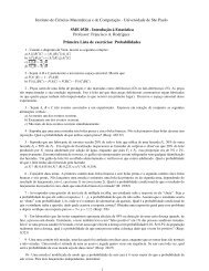
Note that, contrary to what happens in the shortest path problem, an optimal subpath
between two vertices is dependent on the complete path to which it belongs. This happens due
to the hop constraints, as shown in Figure 1. Costs are shown next to the edges. The figure
depicts optimal shortest paths from vertex 1 to the other vertices in the graph, with a hop limit
of 3. Consider the optimal subpath from vertex 1 to vertex 4. This subpath includes vertices
2 and 3 if vertex 4 is the destination, but, in order to respect the hop limit, it includes only
vertex 6 if vertex 5 is the destination. In implementation terms, this means that one must keep
a precedence array for each vertex of the graph vertices while solving the problem.
With an algorithm for the shortest path problem with hop constraints, one can evaluate the
cost of connecting the non-selected profitable vertices to the existing tree and develop a simple
algorithm. Let T be the current solution. At the first iteration, v(T) = {1} and the candidate
destination vertices j are those with L(1,j,h) ≤ b and rj > 0. Note that if a path violates
the hop constraint, the hop constrained shortest path will return ∞, since we stop the dynamic
programming algorithm after h steps. Therefore, paths violating the hop constraint will not
be considered for insertion in the solution. When at least one path has been added, one must
not only consider the new paths that originate at the root vertex, but also all paths that are
originated at other vertices in v(T). The algorithm considers for insertion all shortest paths
such that
L(i,j,h − hi) ≤ b − �
(i,j)∈e(T)
cij, i ∈ v(T),j /∈ v(T),rj > 0.
Instead of running the hop constrained shortest path algorithm for all vertices in the current
solution, we set the costs of the edges in e(T) to 0 and run the algorithm a single time, with
5

6
5
5
Figure 1: Example of different optimal subpaths between two vertices depending on the complete
path.
the root vertex as the origin. Because of the dynamic programming structure, a single run is
able to compute the hop constrained shortest distances from the root to all the other vertices,
saving computation time.
3.2 Evaluating the paths
At each step, a single new path is added to the solution. The criterion used to choose the
path to be added is an important part of the algorithm. If one makes a choice based only on
profits, there is a risk of adding very costly paths that will soon consume the whole budget.
On the other hand, if one chooses to add shortest paths, some vertices with a high revenue but
at a moderate distance from the current solution may be ignored. Based on preliminary tests,
we found that the best strategy was to consider both the costs and the revenues when deciding
on the path to be added. We tested several ratios r α j /cβ , where α and β are two non-negative
numbers, rj is the revenue of the profitable vertex to be added, and c is the sum of the cost of
the edges in the path. We found that the best parameter setting was α = 3 and β = 1, which
was used in all subsequent tests.
Algorithm 1, described in the following figure, presents the complete greedy algorithm in
details. A few comments on this algorithm are in order. First, note that when adding a path one
can also add other profitable vertices in addition to the end vertex. It has proved to be slightly
better not to consider these profits when deciding which path should be added. This way, the
6
1
2
3
4
5
1
1
1
1

Algorithm 1 Greedy algorithm for the STPRBH
1: T is initially the root node: v(T) = {1}.
2: p = 1;
3: while p �= 0 do
4: p = 0,c = 0,j = −1.
5: for all vertices j /∈ v(T) do
6: c = L(1,j,h);
7: p = r 3 j /c.
8: if �
(i,j)∈e(T) cij + c > b then
9: p = 0.
10: end if
11: if p ≥ p then
12: j = j;
13: c = c;
14: p = p.
15: end if
16: end for
17: if p �= 0 then
18: P is the path from 1 to j: P = (i1 = 1,... ,iℓ = j);
19: cit,it+1
= 0, t = 1,... ,ℓ − 1;
20: v(T) = v(T) ∪ v(P);
21: destroy possible cycles.
22: end if
23: end while
24: Return T.
algorithm tends to add shorter paths first, thus reducing the risk of making wrong decisions
due to the myopic character of the choices. Second, because of the hop constraints, one can
sometimes introduce cycles when adding a path. Consider again Figure 1 and the situation
where h = 3, all vertices are profitable and, after the first iteration of the greedy algorithm
v(T) = {1,2,3,4}. Assuming that the budget constraint is not violated, the algorithm will try
to add vertex 5 to the solution, using the edges (1,6) and (6,4) in order to respect the hop
constraint and therefore forming a cycle. When this situation happens, the algorithm destroys
the cycle by inspecting vertices with two incoming edges (in this case, vertex 4) and eliminating
the edge that was inserted first (in this case, edge (3,4)). This way, the cycle is eliminated and
the hop constraints are respected for the entire graph.
7

4 Destroy-and-repair algorithm
The idea of destroying part of the solution and reconstructing it in a different way in order to
obtain different and hopefully better solutions has already been used to solve other combinatorial
problems. Ropke and Pisinger (2006) have employed such a technique to solve vehicle routing
problems with time windows, and Pisinger and Ropke (2007) have applied it to a more general
class of routing problems. Voß (1999) has successfully used a similar idea to solve the STP
with hop constraints. For the STPRBH, we propose a very simple procedure that consists of
sequentially blocking part of the current solution and rerunning the greedy algorithm.
A feasible solution to the STPRBH consists of a tree. Given an initial solution, we simply
set the cost of some edges to infinity, one at a time, and we rerun the greedy algorithm with
the modified costs. This is done for all edges of the current solution that are incident to a
leaf vertex, as shown in Figure 2, and the best obtained solution is retained. The procedure is
repeated for the new solution until there is no gain obtained with the blocking of a single edge.
Algorithm 2 schematically presents the procedure.
Root vertex
Figure 2: Edges incident to leaf vertices.
Edges to be tested
Other ways of preventing the greedy algorithm from repeatedly reaching the same solution
can be used. For example, one could block all edges in the solution, one at a time. We tested
this idea and, although it was much more time consuming, the results were not much better than
the ones obtained with Algorithm 2. In a way this was expected, since the greedy algorithm
8

Algorithm 2 Destroy-and-repair algorithm for the STPRBH
1: T = solution of Algorithm 1;
2: best solution T = T.
3: y = true
4: while y = true do
5: y = false
6: for all the edges (i,j) incident to a leaf vertex do
7: store original cost: cij = cij;
8: cij = ∞;
9: T = solution of Algorithm 1 (with modified costs).
10: if r(T) > r(T) then
11: y = true
12: T = T.
13: end if
14: Restore original cost: cij = cij.
15: end for
16: end while
17: T = T;
18: return T
has a tendency to reconstruct a similar solution if an intermediate edge has been blocked. By
concentrating on the edges incident to profitable leaf vertices we increase the probability of really
blocking that solution and obtaining something new.
We also tested other neighborhoods such as blocking a vertex of the solution (by setting the
cost of all its incident edges to infinity). The results turned out to be worse than those obtained
with the original algorithm. In this case, we think that the explanation comes from the fact
that blocking a vertex is probably too restrictive and by doing so we may eliminate several good
solutions. Finally, we have also tested the possibility of blocking more than one arc at the same
time. Although minor improvements were obtained, the computational times were considerably
larger and this option was also discarded.
5 Tabu search algorithm
A tabu search algorithm was also developed for the STPRBH. The main idea of tabu search
is to define a neighborhood for a solution and let the algorithm explore the search space by
moving to the best allowed neighbor solutions, while defining some forbidden or tabu moves in
9

order to avoid cycling.
We define two basic moves for the STPRBH. The first is an add move. It consists of adding
a path originating at a vertex of the current solution and ending at a profitable vertex. This
is very similar to the basic step of the greedy algorithm presented in Section 3, since this move
also makes use of the shortest path with hop constraints procedure and, therefore, maintains
hop-feasibility during the whole search. In order to increase the flexibility of the algorithm, we
let the add move violate the budget constraint. The idea is to design an algorithm capable of
exploring infeasible parts of the search space in the hope of reaching feasible solutions that could
not be reached otherwise. To encourage the identification of feasible solutions during the search,
a penalty is associated with trees that violate the budget. The idea of letting the tabu search
explore infeasible areas of the search space has been used successfully in other combinatorial
problems (see, e.g., Gendreau et al., 1994).
The second move is remove, which consists of the deletion of a branch of the solution. It is
the counterpart of the add move in the sense that the add move is driven by revenue collection,
while the remove move is driven by budget feasibility. In the following, the two moves are
described in detail. A third move, which is called destroy is also described. We have used this
move only occasionally to help the search algorithm escape from local optima.
With respect to several tabu search implementations developed for the solution of combina-
torial optimization problems, our algorithm is relatively simple. This is a deliberate choice. In
line with Cordeau et al. (2002), we believe it is preferable to design algorithms that are both
accurate and simple. This makes them easy to reproduce and it favours their adoption by other
researchers.
5.1 Add move
An add move is like a single step of the greedy algorithm described in Section 3: one adds the
hop constrained shortest path connecting the best non-selected vertex to the current tree. This
is done by setting the edge costs in the current solution to 0 and running the hop constrained
shortest path procedure, which returns the hop constrained shortest paths originating at the
root and ending at each vertex of the graph. Once a vertex has been added, it is declared tabu
for a number of iterations. This way, the branch connecting the previous solution to the newly
added vertex will not be deleted by the remove move until its tabu status has been lifted.
The tabu mechanism helps avoid cycling and forces the algorithm to explore new areas of
the search space, differentiating the tabu search from the greedy algorithm presented earlier.
Another strategy is used to increase the diversification of the solutions. At each iteration,
one considers only a subset of randomly selected vertices: the algorithm arbitrarily chooses a
10

subset of the possible vertices and adds the best one. Note that this is not done to save any
computational time since the needed information was already available from the hop constrained
shortest path procedure even for the discarded vertices, but as a diversification mechanism.
5.2 Remove move
The remove move consists of eliminating branches of the current solution. It was made
necessary as a counterpart of the add move in order to help the algorithm identify budget-
feasible solutions. We carefully select the branches to be eliminated in order to introduce only
local perturbations in the current solution. This is done by connecting a vertex with degree
larger or equal to three to a leaf of the current tree. For a current solution T, we call B(T) the
set of vertices with degree larger or equal to three. These vertices are called breaking points,
since it is at these vertices that the solution is cut. Figure 3 depicts an example of a tree solution.
The breaking points are highlighted while the possible paths to be cut are shown in dotted lines.
Root vertex
Breaking points
Figure 3: Breaking points and possible paths to be removed
11

5.3 Destroy move
A destroy move that erases a whole subtree of the current solution has also been developed.
This move acts by randomly selecting a vertex in the current solution and deleting the whole
subtree rooted at that vertex. This move was only used after the algorithm spent a certain
number of iterations without improving the best known solution value.
The three moves just described have been incorporated within the tabu search algorithm.
The add and remove moves are evaluated together. First, the gain of all add moves is com-
puted. The gain of one add move connecting the profitable vertex i to the solution is given by
the value of the revenue of the added vertex, minus the difference between the penalties after
and before the move:
γ + i = ri − π(T ′ ) + π(T ′′ ),
where π(T) is the penalty associated with a solution T, and T ′ and T ′′ are the solutions before
and after the move, respectively. For a given solution T with total network cost �
(i,j)∈e(T) cij,
the penalty is given by:
⎧
⎨
π(T) =
⎩
0, if �
(i,j)∈e(T) cij ≤ b
�� φ × (i,j)∈e(T) cij
�
− b , if �
(i,j)∈e(T) cij > b,
where φ is a penalty parameter updated dynamically during the search. The parameter φ is
initialized at 1, but the algorithm is robust with respect to this parameter.
In a complementary manner, the remove move for a node i ∈ B(T) yields a gain equal to:
γ − i = −ri − π(T ′ ) + π(T ′′ ).
At each iteration, the move with the best gain is performed and the penalty parameter φ
is updated. If the new solution is budget feasible, φ is halved, thus encouraging the algorithm
to look for budget-infeasible solutions. Similarly, if the new solution is budget-infeasible, φ is
doubled.
Algorithm 3 presents the tabu search algorithm in detail. It stops after a preset number
of iterations.
6 Computational experiments
We have tested the algorithms just described on several instances obtained from the OR-
Library (Beasley, 1990). The STP instances contain two set of vertices: mandatory vertices
which must be present in the solution, and Steiner vertices which can be used if their inclusion
in the solution reduces the total cost. We have adapted these instances for the STTPBH by
12

Algorithm 3 Tabu search algorithm for the STPRBH
1: T = solution of Algorithm 1;
2: T = T;
3: φ = 1.
4: while stopping criterion not reached do
5: Randomly select a subset R(T) of the profitable vertices not in the tree and compute gain,
γ + i = ri − π(T ′ ) + π(T ′′ ),i ∈ R(T);
6: compute gain for all remove moves, γ − i = −ri − π(T ′ ) + π(T ′′ ),i ∈ B(T);
7: perform move with best gain (γ − i or γ+ i ) and update T;
8: make move tabu for 5 iterations.
9: if solution is budget-feasible then
10: φ = φ/2.
11: if r(T) > r(T) then
12: T = T.
13: end if
14: else
15: φ = 2φ.
16: end if
17: if no improvement in more than 100 iterations then
18: apply destroy move.
19: end if
20: end while
using the mandatory vertices as profitable vertices with revenue given by a discrete uniform
distribution on 1 and 100. The Steiner vertices were attributed a zero revenue. Different values
for the budget and for the hop limit were attributed to each instance, thus creating several
scenarios.
Table 1 summarizes the results obtained for a mid-sized group of 144 instances, ranging
from 50 to 500 vertices and from 63 to 625 edges. Note that for these instances, the exact
methods presented by Costa et al. (2007) were able to converge within a time limit of two hours,
allowing them to be used as benchmarks to evaluate the approximate algorithms. In the table,
for each method (greedy algorithm, destroy-and-repair and tabu search), we report the mean
and maximum gap, as well as the mean and maximum computation times. There are two entries
for the Tabu search algorithm, each corresponding to a maximum allowed number of iterations
(2000 or 10,000). Complete results can be found in Costa et al. (2006a).
Even the simplest of the three algorithms can solve a large number of instances to optimality.
13

Method Gap Max Gap Seconds Max seconds
Greedy 2.50 % 31.97 % < 0.01 0.02
Destroy-and-repair 1.13 % 10.10 % 0.09 1.44
Tabu (2000) 0.52 ± 0.08 % 12.99 ± 7.55 % 0.38 0.90
Tabu (10,000) 0.24 ± 0.05 % 8.46 ± 8.01 % 1.80 4.21
Table 1: Summary of results for the mid-sized instances
Indeed, the greedy algorithm finds an optimal solution for 73 out of the 144 instances. Note that
we did not consider instances with a budget equal to the total network cost since these instances
are easy and the greedy algorithm always finds an optimal solution. It is clear, however, that
for some instances the greedy algorithm can be trapped in a poor quality local optimum. In the
worst of the cases, the algorithm generated a solution with an optimality gap almost equal to
32%. Finally, concerning the computational time, since the algorithm is based on quick shortest
paths calculations, a maximum of 0.02 seconds was required to solve any instance.
Starting from the solution of the greedy algorithm, both the destroy-and-repair and the tabu
search were able to reduce the optimality gaps. The first method reduced the mean gap from
2.50% to 1.13% and the maximum gap from 32% to 10.10%. The tabu search was able to further
reduce these gaps. The mean gap (averaged over ten runs) was reduced to 0.52% when 2000
iterations were allowed, and to 0.24% when 10,000 iterations were allowed. The maximum gaps
for these two cases were 12.99% and 8.46%.
To better evaluate the efficiency of the improvement routines, we consider a second group
of larger instances with up to 500 vertices and 12,500 edges. For these instances, the exact
algorithms described in Costa et al. (2007) generally did not obtain solutions within the allowed
time limit of two hours, often failing to even solve the linear relaxation at the root node. For this
reason, we compare the results obtained by the destroy-and-repair and the tabu search methods
to the results obtained by the greedy algorithm. Table 2 presents a summary of the results. We
can see that even for large instances, the greedy algorithm is very fast, taking on average 1.94
seconds, with a maximum of 31.78 seconds. Still concerning the times, it is interesting to see
how the destroy-and-repair can easily become very computationally inefficient, taking almost
two hours to solve some of the instances. The tabu search, even when run for 10,000 iterations,
is on average 30% faster than the destroy-and-repair algorithm and presents much more stable
computing times. The complete set of results is presented in Costa et al. (2006a).
Concerning the improvements, the destroy-and-repair algorithm yields mean and maximum
improvements of 1.31% and 14.36%, respectively. The tabu search can increase these percentages
to 1.41% and 20.80% when run for 2000 iterations, and obtains considerably better solutions
14

Method Improvement Max improvement Seconds Max seconds
Greedy - - 1.94 31.78
Destroy-and-repair 1.31 % 14.36 % 312.50 6493.60
Tabu (2000) 1.41 ± 0.06 % 20.80 ± 2.60 % 44.98 287.64
Tabu (10,000) 2.00 ± 0.04 % 23.05 ± 2.14 % 237.53 1668.6
Table 2: Summary of results for the larger instances
when 10,000 iterations are allowed. It then yields 2.00% average improvement in comparison to
the greedy algorithm, and a maximum improvement of more than 23%.
7 Conclusions
We have proposed three heuristics for a modified version of the Steiner Tree Problem with
revenues including budget and hop constraints. A former study (Costa et al., 2007) has shown
that exact algorithms based on existing formulations cannot be applied to large instances of
this problem. The heuristics we have proposed are based on simple construction and tabu
search mechanisms. The greedy algorithm is extremely fast but may be trapped in a local
optimum due to its myopic nature. The destroy-and-repair method is a simple modification
of the greedy algorithm which considerably improves its solutions, albeit at the cost of a large
increase in computation time. Finally, the tabu search is capable of consistently identifying
optimal solutions while maintaining the computational times at a reasonable level.
Acknowledgments
This work was supported by the Brazilian Federal Agency for Post-Graduate Education -
CAPES, under grant BEX 1097/01-6 and by the Canadian Natural Science and Engineering
Research Council under grants 227837-04 and OGP0039682. This support is gratefully acknowl-
edged. The authors also thank three anonymous referees for their valuable comments.
References
Avella, P., Villacci, D. and Sforza, A. (2005). A Steiner arborescence model for the feeder
reconfiguration in electric distribution networks, European Journal of Operational Research
164: 505–509.
Balakrishnan, A. and Altinkemer, K. (1992). Using a hop-constrained model to generate alter-
native communication network design, ORSA Journal on Computing 4: 192–205.
15

Beasley, J. E. (1990). OR-Library: Distributing test problems by electronic mail, Journal of the
Operational Research Society 41: 1069–1072.
Canuto, S. A., Resende, M. G. C. and Ribeiro, C. C. (2001). Local search with perturbations
for the prize-collecting Steiner tree problem in graphs, Networks 38: 50–58.
Carneiro, M. S., França, P. and Silveira, P. D. (1996). Long-range planning of power distribution
systems: secondary networks, Computers and Electrical Engineering 22(3): 179–191.
Cordeau, J.-F., Gendreau, M., Laporte, G., Potvin, J.-Y. and Semet, F. (2002). A guide to
vehicle routing heuristics, Journal of the Operational Research Society 53: 512–522.
Costa, A. M., Cordeau, J.-F. and Laporte, G. (2006a). Fast heuristics for the Steiner tree
problem with revenues, budget and hop constraints, Publication CRT-2006-16, Centre for
Research on Transportation, Montreal .
Costa, A. M., Cordeau, J.-F. and Laporte, G. (2006b). Steiner tree problems with profits,
INFOR 44: 99–115.
Costa, A. M., Cordeau, J.-F. and Laporte, G. (2007). Models and branch-and-cut algorithms
for the Steiner tree problem with revenues, budget and hop constraints, Networks (forth-
coming) .
Cunha, A. S., Lucena, A., Maculan, N. and Resende, M. G. C. (2003). A relax and cut al-
gorithm for the prize collecting Steiner problem in graphs, Proceedings of Mathematical
Programming in Rio, Búzios, Brazil : 72–78.
Gendreau, M., Hertz, A. and Laporte, G. (1994). A tabu search heuristic for the vehicle routing
problem, Management Science 40: 1276–1290.
Gouveia, L. (1995). Using the Miller-Tucker-Zemlin constraints to formulate a minimal spanning
tree problem with hop constraints, Computers & Operations Research 22: 959–970.
Gouveia, L. (1996). Multicommodity flow models for spanning trees with hop constraints,
European Journal of Operational Research 95: 178–190.
Gouveia, L. (1998). Using variable redefinition for computing lower bounds for minimum span-
ning and Steiner trees with hop constraints, INFORMS Journal on Computing 10: 180–188.
Gouveia, L. and Magnanti, T. L. (2003). Network flow models for designing diameter-constrained
minimum-spanning and Steiner trees, Networks 41: 159–173.
16

Gouveia, L. and Requejo, C. (2001). A new Lagrangean relaxation approach for the hop-
constrained minimum spanning tree problem, European Journal of Operational Research
132: 539–552.
Lawler, E. (1976). Combinatorial Optimization: Networks and Matroids, Holt, Rinehart and
Winston, New York.
LeBlanc, L., Chifflet, J. and Mahey, P. (1999). Packet routing in telecommunication networks
with path and flow restrictions., INFORMS Journal on Computing 11: 188–197.
Ljubić, I., Weiskircher, R., Pferschy, U., Klau, G., Mutzel, P. and Fischetti, M. (2005). Solving
the prize-collecting Steiner tree problem to optimality, Proceedings of ALENEX, Seventh
Workshop on Algorithm Engineering and Experiments, Vancouver .
Pisinger, D. and Ropke, S. (2007). A general heuristic for vehicle routing problems, Computers
& Operations Research (forthcoming) .
Ropke, S. and Pisinger, D. (2006). An adaptive large neighborhood search heuristic for the
pickup and delivery problem with time windows, Transportation Science (forthcoming) .
Voß, S. (1999). The Steiner tree problem with hop constraints, Annals of Operations Research
86: 321–345.
Voß, S. (2006). Steiner tree problems in telecomunications, in P. Pardalos and M. G. C. Resende
(eds), Handbooks of Telecommunications, Springer, New York .
17