Chapter 3 - Controllability and Observability - University of Minnesota

University of Minnesota ME 8281: Advanced Control Systems Design, 2001-2012 69
Output
2.5
2
1.5
1
0.5
0
−0.5
−1
measured
uncorrupted
estimate
−1.5
0 1 2 3 4 5
Time(sec)
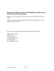
Figure 3.13: Least squares estimate
This means that the observer gain L(t) will decrease. The observer will asymptotically rely
more and more on open loop estimation:
Output
3
2
1
0
−1
d
ˆx(t|t) =A(t)ˆx(t|t)
dt
measured
uncorrupted
λ = 1.5
λ = 5
−2
0 1 2
λ = 10
3 4 5
Time(sec)
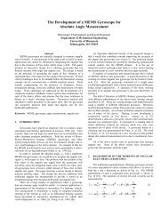
Figure 3.14: Least squares estimate with forgetting factor

University of Minnesota ME 8281: Advanced Control Systems Design, 2001-2012 81
3.15 Realization
3.15.1 Transfer Function to State-space model
The models of many physical systems are more conveniently obtained in the transfer function form.
In order for us to implement state-space control design techniques, it is essential that we have a
state-space representation. It should be noted that there is no unique state-space realization for a
transfer function, since any set of states can be used. However, there are some realizations that are
“canonical”, or simplest. The “first companion” or “controllable canonical” form is given here.
The transfer function for a SISO system
can be written
H(s) =
Y (s)
U(s) =
Using inverse Laplace transform, the D.E. is
1
s n + a1s n−1 + a2s n−2 + ···+ an
(3.17)
(s n + a1s n−1 + a2s n−2 + ···+ an)Y (s) =U(s) (3.18)
D n y + a1D n−1 y + ···+ any = u D n ≡ dn
dt n
(3.19)
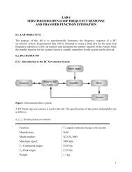
Each term, starting from the second, is an integration of the preceding term. So, the relationship
can be expressed as a chain of integrators, as shown in Fig. 3.17. The output of each integrator is
designated a state variable, from right to left. So, the output of the n th integrator is x1, whichis
the same as the system output y.
u
−
i i i i
xn
xn1
a1 a2 an1 an
Figure 3.17: First companion form (ref: Control System Design, B. Friedland)
This can be represented as a set of n linear D.E.’s
˙x1 = x2
˙x2 = x2
.
˙xn−1 = xn
˙xn = −anx1 − an−1x2 −···−a1xn + u
x2
x1
y