A Design Tool for Aerodynamic Lens Systems - Department of ...

Aerosol Science and Technology, 40:320–334, 2006 

Copyright c○ American Association for Aerosol Research 

ISSN: 0278-6826 print / 1521-7388 online 

DOI: 10.1080/02786820600615063 

A Design Tool for Aerodynamic Lens Systems 

Xiaoliang Wang 1,2 and Peter H. McMurry 1 

1 Department of Mechanical Engineering, University of Minnesota, Minneapolis, Minnesota, USA 

2 Current address: TSI Inc., St. Paul, Minnesota, USA 

We report in this article the development of a tool to design and 

evaluate aerodynamic lens systems: the Aerodynamic Lens Calculator. 

This Calculator enables quick and convenient design of 

aerodynamic lens systems based on the parameterized knowledge 

gained from our detailed numerical simulations of flow and particle 

transport through aerodynamic lens systems. It designs the key 

dimensions of a lens system: pressure limiting orifice, relaxation 

chamber, focusing lenses, spacers and the accelerating nozzle. It 

also provides estimates of particle terminal axial velocities, particle 

beam width, and particle transmission efficiencies. This article 

describes in detail the information that is used in the design tool, 

including equations for pressure drop through orifices, contraction 

factors as a function of Reynolds, Mach and Stokes numbers, 

spacer length as a function of Reynolds number and estimations 

for the relaxation chamber dimensions. The article also evaluates 

the performance of the design tool by comparing its predictions 

with the performance of aerodynamic lens systems that have been 

described in the literature. 

[Supplementary materials are available for this article. Go to the 

publisher’s online edition of Aerosol Science and Technology for the 

following free supplemental resources: An instruction manual for 

the Aerodynamic Lens Calculator.] 

INTRODUCTION 

Aerodynamic lens systems have been widely used to generate 

collimated narrow particle beams since they were invented 

by Liu et al. (1995a, b). Typical applications include inlets for 

aerosol mass spectrometers (Ziemann et al. 1995; Schreiner et al. 

1998, 1999, 2002; Jayne et al. 2000; Tobias et al. 2000; Öktem 

et al. 2004; Su et al. 2004; Svane et al. 2004; Drewnick et al. 

2005; Zelenyuk and Imre 2005), nanostructured material synthesis 

(Girshick et al. 2000; Dong et al. 2004; Piseri et al. 2004), and 

micro-scale device fabrication (Di Fonzo et al. 2000; Gidwani 

2003). 

In the original design of the aerodynamic lens system (Liu 

et al. 1995a, b), aerosols are sampled from one atmosphere pres- 

Received 23 November 2005; accepted 3 February 2006. 

This work was supported by NSF (Grant No. DMI-0103169) 

and the University of Minnesota Supercomputing Institute. We thank 

Dr. Frank Einar Kruis for helpful discussions. 

Address correspondence to Peter H. McMurry, 111 Church Street 

SE, Minneapolis, MN 55455, USA. E-mail: mcmurry@me.umn.edu 

320 

sure through a pressure limiting orifice into the lenses which 

operate at a pressure of ∼200 Pa, with low pressure drop across 

each lens. Typically a series of three to five lenses progressively 

focus spherical particles in the size range of 25–250 nm (near 

unit density) into a narrow beam. The collimated particle beam 

is then delivered through an accelerating nozzle to the detection 

chamber maintained at very low pressure. Most lens systems 

being used today are similar in design to the system described 

by Liu et al. (1995a, b). 

Several studies have reported on lens systems that were designed 

to operate under conditions that are significantly different 

from those used by Liu et al. (1995 a, b). For example, Di Fonzo 

et al. (2000) designed a lens system to focus silicon carbide 

particles in the diameter range of 10–100 nm using an argonhydrogen 

mixture; Dong et al. (2004) used a lens system to focus 

10–200 nm silicon particles in hydrogen. Schreiner et al. developed 

aerodynamic lens systems operating at elevated pressures 

(2.5–20 kPa) for stratospheric aerosol studies (Schreiner et al. 

1998, 1999, 2002). Lee et al. (2003) used a single lens to focus 

micron-sized particles in the atmospheric pressure range. Wang 

et al. (2005a, b) developed a systematic procedure to design 

aerodynamic lenses for 3–30 nm nanoparticles. 

To characterize the performance of an aerodynamic lens system, 

detailed numerical or experimental studies are required. Liu 

et al. (1995a, b) carried out theoretical, numerical, and experimental 

analysis of the performance of aerodynamic lens systems. 

Zhang et al. (2002, 2004) repeated the simulations by Liu 

et al. with a compressible flow model. To study particle loss and 

beam broadening due to diffusion, Gidwani (2003) and Wang 

et al. (2005b) simulated the flow and particle transport in the 

lens system considering the particle Brownian motion. 

Although numerical simulations or experimental evaluation 

of the performance of lens systems can provide more accurate 

results, they are very costly in both time and financial resources. 

Furthermore, these studies require predefined dimensions and 

operating conditions of the aerodynamic lens system, which 

need to be iteratively optimized. Due to the wide applications of 

aerodynamic lenses, a simple tool that can provide quick and reasonably 

accurate lens design and evaluation would be useful. We 

report the development of such an Aerodynamic Lens Calculator 

in this article. We studied flow and particle transport through 

a single lens at a wide range of Reynolds and Mach numbers.

From these simulations, we obtained information about particle 

contraction factors, transport efficiencies, flow discharge coefficients 

through orifices and the lengths of spacer for flow to 

redevelop. We also simulated flow through the pressure limiting 

orifice and the relaxation region, the accelerating nozzle, as 

well as the entire lens system (Wang 2005b). Results from these 

detailed numerical calculations were parameterized and incorporated 

into the design tool described in this paper. We correlated 

the particle terminal axial velocity in the vacuum chamber 

downstream of the nozzle as a function of Stokes number with a 

simple equation. This enabled us to estimate the particle terminal 

axial velocity under similar nozzle geometry and operating 

pressure. We also provide estimate of the particle beam width 

both inside and downstream of the lens system. Both aerodynamic 

focusing and diffusion broadening are taken into account 

in the beam width estimation. We considered three particle loss 

mechanisms to calculate the particle transport efficiency: inertia 

impaction on the orifice plate, impaction on the spacer walls due 

to defocusing, and losses due to diffusion. 

This design tool avoids the need for the time consuming detailed 

numerical simulations, and enables designers to quickly 

test a range of design options. The tool calculates the lens dimensions, 

operating conditions and flow parameters at each 

lens stage. It also estimates the terminal particle velocity after 

the choked accelerating nozzle, particle beam diameter at each 

stage and at the location of the detector, and particle transport 

efficiency through the lens system. This article describes the detailed 

information used in the Calculator. We first describe the 

analytical, empirical or numerical relations used to design the 

dimensions and operating conditions of aerodynamic lens systems. 

Next we describe the method used to estimate the particle 

terminal velocity, beam width and transport efficiency. Finally, 

we report the validation of this lens design tool by comparing 

its predictions with several detailed numerical and experimental 

studies reported in the literature. 

AERODYNAMIC LENS SYSTEM DESIGN 

The objective of aerodynamic lens design is to build a 

lens system that has best performance, i.e., maximum particle 

focusing, minimum particle losses, and minimum pumping 

A DESIGN TOOL FOR AERODYNAMIC LENS SYSTEMS 321 

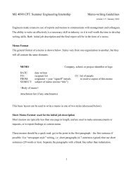
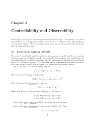
FIG. 1. Schematic and nomenclatures of the lens system. 

requirements under user specified inputs (particle size range, 

particle density, etc.). To achieve this goal, one needs to optimize 

dimensions of the lens system (number of lenses, lens diameters, 

inner diameter and length of the spacers between two 

lenses, the flow limiting orifice, relaxation chamber and the accelerating 

nozzle) and operating parameters (flowrate, pressure, 

and carrier gas). 

We have briefly described the aerodynamic lens design procedure 

in an earlier article with emphasis on lenses for nanoparticles 

(Wang et al. 2005a). In this section, we describe the design 

principle in more detail, and generalize the guidelines to be applicable 

to particles ranging in size from several nanometers to 

greater than one micrometer. 

Assumptions 

Figure 1 shows a schematic of an aerodynamic lens system 

with the nomenclature used in this paper and in the code of the 

lens calculator. The lens system described in this article consists 

of the following parts: an inlet orifice followed by a relaxation 

chamber, one or more lenses separated by spacers, and an accelerating 

nozzle. The pressure limiting orifice determines the 

volumetric flowrate through the lens system, and the accelerating 

nozzle defines the operating pressure. We assume that the 

lenses are primarily responsible for all focusing. The focusing 

or defocusing effects that might be caused by the inlet orifice 

or the accelerating nozzle are not controlled by the design tool, 

but the user can optimize these effects by varying the operating 

pressure. The inner diameters of each spacer are usually the 

same so as to simplify machining. 

Particles are assumed to be spherical and electrically neutral. 

The effects of particle shape have been discussed by Liu et al. 

(1995a, b) and Huffman et al. (2005). The design tool restricts 

flow through the lenses to be laminar, subsonic, and continuum. 

It is well known that flow instability and turbulence can disperse 

particles and destroy focusing. However, the Reynolds 

number above which these effects contribute to defocusing is not 

known with certainty. Eichler et al. (1998) and Gómez-Moreno 

et al. (2002) reported that turbulent transition in an orifice flow 

occurred at Reynolds number around 70. Back and Roschke 

(1972) and Gong et al. (1996) found flow instabilities around

322 X. WANG AND P. H. MCMURRY 

aReynolds number of 200 downstream of sudden expansions. 

Our design tool constrains Reynolds numbers (Re) tobebelow 

200. Therefore, 

Re = ρ1ud f 

µ = 4 ˙m 

πµd f 

≤ 200. [1] 

Although sonic or supersonic nozzles have been widely used 

to focus particles (Murphy and Sears 1964; Israel and Friedlander 

1967; Cheng and Dahneke 1979; Dahneke and Cheng 1979; 

Fernández de la Mora et al. 1989; Mallina et al. 2000; Tafreshi 

et al. 2002), we constrain the flow through lenses to be subsonic 

to avoid the complicated influence of shock waves on particle 

focusing. Therefore, the lens Mach number (Ma) islimited to 

be smaller than the value corresponding to choked flow (Ma ∗ ) 

(Wang et al. 2005a), i.e., 

Ma = u 

c < Ma∗ . [2] 

If the flow is in the free molecular regime, the particle inertia 

would greatly exceed the drag force and no focusing could be 

achieved. Furthermore, rarefied gas dynamics is too complicated 

to handle using our simple design tool. Therefore, we restrict the 

flow Knudsen number (Kn)tobesmaller than 0.1 to assume that 

the flow is continuum, 

Kn = 2λ1 

d f 

< 0.1. [3] 

Focusing Lens 

The parameter that governs particle focusing through an aerodynamic 

lens is the Stokes number (St), which is defined as the 

ratio of the particle stopping distance at the average orifice velocity 

(u) tothe orifice diameter (d f ): 

St = τu 

d f 

= 2ρpd 2 pCc ˙m 

9πρ1µd3 , [4] 

f 

where Cc = 1 + Knp(1.257 + 0.4e −1.1 

Knp ) and Knp = 2λ1/dp. 

As shown in earlier studies, the particle contraction factor (ηc), 

which is the ratio of terminal to initial radial positions of the 

particles travelling through the lens, is a strong function of the 

Stokes number: |ηc| ≈1 when St ≪ 1, |ηc| < 1 when St ≈ 1, 

and |ηc| > 1 when St ≫ 1. In other words, small particles 

follow gas streamlines and thus are not focused, intermediatesized 

particles are focused and large particles are defocused by 

the lens. There exists an optimum Stokes number (Sto) for which 

ηc = 0 (Liu et al. 1995a). Liu et al. showed that the contraction 

factors are independent of the particle initial radial position for 

particles that are not too far away from the axis. We refer to these 

near-axis contraction factors unless stated otherwise. 

By rearranging Equation (4), we can calculate the diameter 

of the lens aperture for optimally focused particles: 

� 

2ρpd 

d f = 

2 pCc � 1 

˙m 3 

. [5] 

9πρ1µSto 

Note that the optimal Stokes number is a function of flow 

Reynolds number, Mach number, and lens geometry (Liu et al. 

1995a; Zhang et al. 2002). We use thin plate orifices as the focusing 

elements in this paper. Liu et al. (1995a) showed that 

the dependence of Sto on the constriction ratio (β)ofthin plate 

orifices becomes weak when β ≤ 0.25. To simplify the design 

process, we use β ≤ 0.25 in the design tool. In principle, one 

could use β>0.25 if the ηc vs. St curves were known. 

To obtain the relation between Sto, Ma, and Re, wehave 

carried out numerical simulations of particle motion through a 

single lens at a range of Mach number (Ma = 0.03–0.32) and 

Reynolds numbers (Re = 1–100) which cover the typical operating 

conditions of lenses. In these simulations, β was set equal 

to 0.2. Particles were injected at an initial radial location (r pi)of 

0.15ds from the lens axis and Brownian motion was neglected. 

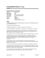
The relationship between the contraction factor and St, Re, and 

Ma is shown in Figure 2(a)–(c). Note that the dependence of 

contraction on Reynolds number decreases as Mach number 

increases. The dependence of the contraction factor on the particle 

initial radial location becomes significant for large Stokes 

numbers (Liu et al. 1995a). Therefore, the near-axis contraction 

factors in Figure 2 are not very representative at the higher St end 

of each curve, and significant impaction losses occur for particles 

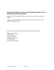
with St > 10. Figure 3 shows the optimum Stokes number 

Sto as a function of Re for three different Ma, which corresponds 

to the St where ηc = 0ateach curve in Figure 2. The value of 

Sto for a specific set of Re and Ma can be interpolated from this 

data. 

From Equation (5), we can see that the pressure upstream 

of the lens is an important parameter in calculating the lens 

diameter. Therefore, we need to accurately estimate the pressure 

drop across an orifice. We have developed a model for viscous 

flow through an orifice 

CdY � 

˙m = A f � 2ρ1(p1 − p2) 

1 − β4 CdY 

= A f � 

1 − β4 p1 

� 

2M �p 

RT1 p1 

as well as for the discharge coefficient (Wang et al. 2005a) 

Cd = 

⎧ 

0.1373Re 

⎪⎨ 

⎪⎩ 

0.5 (Re < 12) 

1.118 − 0.8873 × Ln(Re) + 0.3953 × [Ln(Re)] 2 

− 0.07081 × [Ln(Re)] 3 

+ 0.005551 × [Ln(Re)] 4 − 0.0001581 × [Ln(Re)] 5 

(12 ≤ Re < 5000) 

0.59 (Re ≥ 5000) [7] 

[6]

FIG. 2. Near-axis particle contraction factor as a function of the Stokes number 

for various Reynolds numbers at three different subsonic Mach numbers. 

(a) Ma = 0.03; (b) Ma = 0.10; (c) Ma = 0.32. 


FIG. 3. Optimum Stokes number as a function of Reynolds number for three 

different Mach numbers. 

The expansion factor Y is calculated using the expression of 

(Bean 1971): 

Y = 1 − (0.410 + 0.350β 4 ) �p 

. [8] 

γ p1 

Using Equations (5–8) we can calculate the diameter of each 

lens for a given mass flowrate and a pressure at any stage of the 

lens assembly. 

To study the particle size range that a multiple lens system 

can focus, we found from Equation (4) that in the free molecular 

regime St is proportional to dp while in the continuum regime 

it is proportional to d2 p .Ifalens system focuses particles of a 

decade size range dp1–dpN with dp1 = 10dpN, then the Stokes 

number of dp1 at the last lens will be 10Sto if it is in the free 

molecular regime, and 100Sto if it is in the continuum regime. If 

by any non-ideal effects particles of dp1were not focused exactly 

onto the axis, they will start to defocus at the last lens or even at 

an earlier stage. Therefore, it is probably a good idea to design 

a lens system to cover approximately a decade of particle size. 

Substantial focusing can be achieved even with sub-optimal 

Stokes numbers when a sufficient number of lenses are used. 

There are two strategies to focus a wider range of particle sizes. 

First, one can add additional lenses to refocus the larger particles 

before they are defocused and lost. Second, one can use 

first several lenses to focus the largest particles (dp1) toagiven 

tolerance close to the axis, and then design the following lenses 

at ηc(dp1) =−1 and focus smaller sizes sub-optimally. 

If particles are large enough that diffusion is not significant, 

and the largest particles do not defocus in the final stages, 

the more lenses used in an assembly, the better focusing can 

be achieved. In practice, however, increasing the number of 

lenses increases the difficulty of alignment and adds size and expense. 

Effects of diffusion increase as the lens length increases.


Furthermore, larger particles are more prone to be defocused in 

an assembly with more lenses. Typically, we have found that a 

lens assembly consisting of five lenses is sufficient to focus particles 

of a decade size range. Three or four lenses were used in 

our previous study of nanoparticle focusing (Wang et al. 2005b). 

Operating Pressures 

From Equation (4), we obtain the pressure (pfocusing) for focusing 

particles dp using the ideal gas law 

pfocusing = 2ρpd 2 p Cc ˙mRT 

9πµd 3 f MSto 

. [9] 

Note that Cc is a function of pfocusing. The minimum pressure for 

flow to be subsonic (pMa) and continuum (pKn) are respectively 

given as (Wang et al. 2005a) 

and 

˙mc 

pMa = 

CdYc A f 

pKn = 

2 T1 

λr 

d f Kn∗ Tr 

� � 

2M 

pr 

RT1 

xc 

[10] 

1 + S/Tr 

. [11] 

1 + S/T1 

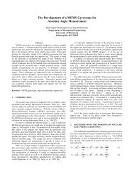
Figure 4 shows examples of pMa, pKn, and the required pfocusing 

to focus particles of different sizes as functions of the orifice size 

in Figure (4a) air and Figure (4b) helium when the flowrate is 0.1 

standard liter per minute (slm). The lens operating pressures are 

those along the pfocusing curves where pfocusing is wider than both 

pMa and pKn. Note that larger particles have a larger operating 

pressure window, and that using a lighter carrier gas can increase 

the operating pressures for smaller sizes which enables focusing 

them. Also shown in Figure 4(a) is a “Re warning line,” which 

corresponds to Re = 200 above which turbulence is likely to 

degrade focusing. 

As was pointed out previously (Wang et al. 2005a), increasing 

the operating pressure can reduce the detrimental effects of 

nanoparticle diffusion and can reduce the pumping needs. From 

Figure 4, we can see that the maximum operating pressure of 

smaller sizes occurs where the pMa curve intersects the pfocusing 

curve for each particle size, and its value can be derived from 

Equations (9) and (10), 

pmax = 648 ˙mµ2 St 2 o 

πC 3 d Y 3 c ρ2 p d4 p C2 c 

� 

M 

2RTx 3 c 

. [12] 

Note that this is an implicit expression because Cc is a function 

of pmax, and an iterative method is needed to calculate pmax. 

The pMa curve may not intersect the pfocusing curve for larger 

particles in the practical orifice diameter range. In this case any 

value of pfocusing larger than pKn can be used. However, Figure 4 

FIG. 4. The operating pressures for focusing unit density particles of different 

sizes as a function of orifice size using (a) air and (b) helium as the carrier gas. 

The flowrate is 0.1 slm. The two dash lines are the lower pressure limits pMa 

and pKn, respectively. The solid lines are pfocusing for indicated sizes. 

shows that the higher the operating pressure, the larger is the 

Reynolds number. It follows that Reynolds numbers tend to limit 

the maximum pressure at which lenses can be operated. 

Length of Spacers 

Spacers are used to separate lenses. They provide room for 

generating the periodic converging/diverging flow pattern with 

orifices, which drives aerodynamic focusing. In addition to the 

constraints mentioned earlier (β ≤ 0.25; equal inner diameter of 

all spacers), the spacers should be long enough so that the flow 

from the preceding lens can relax back to fully developed pipe 

flow before reaching the next lens (Liu et al. 1995b). Typically, 

spacer lengths are 10–50 times the upstream orifice diameter 

depending on the orifice Reynolds number (Wang et al. 2005a). 

However, no quantitative guideline on the spacer length has been 

reported.

Figure 5 shows the flow field through two lenses separated 

by a spacer. The flow separates from the wall when it passes 

through the lens and a recirculation zone forms downstream 

of the orifice. After a distance lr (reattachment length), the flow 

reattaches to the wall, and becomes fully developed at a distance 

of l f (redevelopment length) downstream of the orifice. The 

existence of the downstream lens is felt by the flow la (approach 

length) upstream of the next lens where the flow starts to curve 

toward the centerline. Ideally, the minimum length of spacers 

(ls) should be ls1 = lr + la, and more safely, ls2 = l f + la. 

If the spacer length is less than ls1, the recirculation zone will 

likely fill the whole length of the spacer and less focusing will 

occur. Furthermore, particles are more likely to be entrained in 

the recirculation zones and be lost to the wall. Therefore, when 

particle diffusion is negligible and the overall length of the lens 

system is not a concern, we suggest using spacer lengths at 

least ls2. When diffusion is important, ls1 < ls ≤ ls2 can be 

used. 

To estimate the values of lr, l f , and la,wehave carried out numerical 

simulations of flow through single lenses in the Reynolds 

number range of 0.1–200. Calculated values for lr are shown in 

Figure 6, together with data provided by other researchers (Back 

and Roschke 1972; Oliveira et al. 1998). Note that our numerical 

results are very close to those by Oliveria (1998), which apply 

to similar Reynolds numbers and expansion ratios. The results 

by Back et al. differ somewhat from ours and those of Oliveria, 

probably due to the difference in ER. Since we did not carry out 

simulations for Re > 200, we will use the data by Back et al. 

to estimate lr in this Re range, noting that applying Back’s data 

(ER = 2.6) to larger ER values might lead to some error. Also 

shown in Figure 6 is a fitted curve to the whole Reynolds number 

range, which can be described as follows 

lr 

h = 

⎧ 

−1.016 × 10 

⎪⎨ 

⎪⎩ 

−6 Re3 + 3.150 × 10−4 Re2 + 8.407 

× 10−2 Re + 0.3689 

� 

for Re ≤ 200 

9.096 + 3860.168 × exp − log10 (Re) 

� 

.[13] 

� 

� 0.431 

× sin − 4.226 for Re > 200. 

2π log 10 (Re) 

1.272 


FIG. 5. Streamlines through two lenses separated by a spacer. 

The redevelopment length l f can be estimated by l f = lr + le 

where le is given as (Young et al. 2000) 

le 

dt 

� 

0.06Res for 0 ≤ Res < 2300 

= 

. [14] 

for Res ≥ 2300 

4.4Re 1 

6 

s 

The approach length la is found in our simulation to be independent 

of Reynolds number (Re < 150) with 

la/h ≈ 1.625. [15] 

Since la is relatively shorter than lr and l f ,weuse the above 

equation to estimate la for the whole Reynolds number range. 

Flow Limiting Orifice, Relaxation Chamber, 

and Accelerating Nozzle 

The flow limiting orifice, relaxation chamber, and the accelerating 

nozzle are important components of the aerodynamic 

FIG. 6. Reattachment length of flow downstream of an axisymmetric 

expansion.


lens system. The flow limiting orifice and relaxation chamber 

are required if the particle source pressure is higher than the 

lens operating pressure. The orifice sets the volumetric flowrate 

through the lens system, and reduces the pressure to the lens 

operating pressure. Usually the flow through the flow limiting 

orifice is critical. Therefore, a relaxation chamber is needed to 

slow down the high velocity flow and particles to prevent particle 

impaction on the downstream lens. The relaxation chamber 

also provides space for the flow to reattach to the wall after the 

recirculation eddies downstream of the orifice. The accelerating 

nozzle controls the exact lens operating pressure, and it accelerates 

particles to a downstream destination with minimized 

divergence angles. 

The inner diameter of the relaxation chamber can be estimated 

from the radial stopping distance of the largest particles 

of interest. The lower half of Figure 7(a) shows the flow streamlines 

downstream of a straight-bored critical orifice with a diameter 

and wall thickness of 0.1 mm. The inlet pressure is 1 

atm and the outlet pressure is 266 Pa. The flowrate is 70.6 sccm, 

which correspond to a Reynolds number of 1071 based on the 

orifice diameter. Therefore, the jet is turbulent. However, for the 

sake of simplicity, we only used a steady laminar flow model 

in this simulation and hence the streamlines in Figure 7(a) only 

serve as a qualitative description of the averaged flow behavior. 

The upper half of Figure 7(a) shows the half jet opening angle 

θ, which is defined as θ = tan −1 (h/lr) ≈ tan −1 (vr/va). Assuming 

va equals the speed of sound c, then vr ≈ c tan(θ). We 

further conservatively assume that particle velocity equals to the 

FIG. 7. Straight bored critical orifice and cylindrical relaxation chamber. 

(a) Flow streamlines and illustration of the half jet opening angle; (b) Trajectories 

of 100 nm (above axis) and 1 µm (below axis) particles. 

flow velocity, then the particle radial stopping distance can be 

estimated from Sr = τvr where τ is the relaxation time of the 

largest particles in the target focusing size range downstream of 

orifice. The minimum diameter of the relaxation chamber (dr) 

is then 

dr = 2Sr + d f . [16] 

Here d f is the diameter of the critical orifice. 

The relaxation chamber should be long enough to let flow 

reattach and particles slow down. The length l f for flow to redevelop 

can be calculated using Equations (13) and (14). Due to 

the complicated shock structure, we assume that particles have 

velocities equal to the speed of sound c for the carrier gas at a 

distance lr downstream of the orifice while the gas velocity is 

negligibly low. The particle axial stopping distance downstream 

of lr is then Sa = τc. Therefore, the length of the relaxation 

chamber Lr can be estimated as 

Lr = max(l f + la, lr + Sa). [17] 

The shape of the relaxation chamber and critical orifice aperture 

are also important to reduce particle losses. Figure (7b) 

shows trajectories of 100 nm (above the axis) and 1 µm (below 

the axis) particles through the critical orifice. The turbulent 

dispersion of particles is not included in the simulation. Note 

that some particles of both sizes are trapped inside the recirculation 

region for a long time, which makes them susceptible 

to coagulation or deposition losses. Therefore, we recommend 

that the strong recirculation region be eliminated. This 

can be achieved by inserting a conical expansion downstream 

of the orifice as shown in Figure 8(a). Figure 8(b) shows trajectories 

of 100 nm and 1 µm particles through this modified 

relaxation chamber. Although this new design eliminates 

the recirculation eddy, impaction losses for larger particles increase 

due to the narrowed flow path, as is illustrated by the 

1 µm trajectories. To reduce impaction losses of larger particles, 

one can use conical nozzles, short capillaries or their 

combinations instead of thin plate orifices, since these nozzle 

shapes will reduce particle accelerations at the nozzle inlet 

(Fernández de la Mora and Riesco-Chueca 1988; Fernández de 

la Mora et al. 1989). Figure (8c) illustrates that impaction losses 

of 1 µm particles are reduced by adding a 0.1 mm thick 45 ◦ 

chamfer to the original orifice. (Note that this orifice modification 

increases the flowrate by 10.4%.) Although we demonstrated 

methods to improve the performance of the relaxation 

region in this section, we should point out that more careful 

studies of the orifice shape and chamber dimensions are still 

required. 

We follow the recommendation of Liu et al. (1995b) to use 

a step nozzle as the accelerating nozzle of lens systems (see 

Figure 1). The diameter of the final orifice in the nozzle can 

be calculated using Equation (6), and other dimensions of the 

nozzle are taken as dt ≈ 2dn, Lt ≈ ds.Again, further research is

FIG. 8. Modified relaxation chamber with a conical divergent section to reduce 

recirculation and particle loss. (a) Flow streamlines (straight orifice); (b) 

Trajectories of 100 nm (above axis) and 1 µm (below axis) particles (straight 

orifice); (c) Trajectories of 100 nm (above axis) and 1 µm (below axis) particles 

(orifice with a chamfer). 

needed to optimize the nozzle design so that the nozzle can also 

achieve maximum focusing for a given size range and operating 

conditions. 

LENS PERFORMANCE ESTIMATION 

The most important performance parameters for an aerodynamic 

lens system are: particle terminal velocities, particle beam 

widths at various locations, and the particle transmission efficiencies. 

These parameters need to be evaluated by detailed numerical 

simulations, and ultimately by experiments. However, 

it is attractive to have a best estimation of the lens performance 

with a “one-button-click” effort during the design process. In 

this section, we describe the method used in the Lens Calculator 

to do the estimations. 


FIG. 9. Normalized particle terminal axial velocities downstream of several 

aerodynamic lens systems. 

Estimation of Particle Terminal Velocities 

We assume that the pressure downstream of the accelerating 

nozzle is low enough so that the gas-particle collisions are 

negligible and particles achieve their “terminal” velocities. We 

further assume that particles are in thermal equilibrium with the 

carrier gas upstream of the nozzle exit and their radial velocity 

can be approximately described by the Maxwell-Boltzmann distribution. 

This velocity distribution can be assumed to be frozen 

during the expansion downstream of the nozzle (Liu et al. 1995a; 

Wang et al. 2005b). Therefore, the terminal radial velocity vpr 

can be estimated as 

f (vpr)dvpr = m � 

p 

exp − 

2πkTpF 

m pv2 � 

pr 

2π vpr dvpr. [18] 

2kTpF 

The particle terminal axial velocities (u p) depend on particle 

size, shape, nozzle geometry, pressure ratio, and carrier gases 

(Cheng and Dahneke 1979; Dahneke and Cheng 1979; Mallina 

et al. 1997). Figure 9 summarizes the particle terminal axial velocities 

for the four aerodynamic lens systems listed in Table 1. 

These four lens systems differ in dimensions, flowrate, pressure, 

and carrier gas. But they all use step accelerating nozzles similar 

to that described by Liu et al. (1995b), and the pressures downstream 

of the nozzles are less than 1 Pa. Note that the following 

equation fits the data points reasonably well in the St = τ c/dn 

range where data is available (0.01 < St < 80) 

u p/c = (0.939 + 0.09St)/(1 + 0.543St). [19] 

We will use this equation to estimate particle axial velocity in 

the Lens Calculator.


TABLE 1 

Key features of four lens assemblies with step accelerating nozzles used in particle axial velocity comparison 

Lens system dn (mm) ds (mm) dt (mm) Lt (mm) Gas p1 (Pa) dp (nm) 

A(Wang et al. 2005b) 2.76 10 6 5 He 528 3–30 

B (Liu et al. 1995b) 3.0 10 6 10 Air 93–333 25–250 

C (TSI AFL-050) 3.2 17.78 7.62 17.78 Air 250 50–500 

D (TSI AFL-100) 1.48 17.78 7.62 17.78 Air 600 100–3000 

Estimation of Particle Beam Widths 

The particle beam width is defined as the beam diameter that 

encloses 90% of the total particle flux. In this section expressions 

are given that are used in the Calculator to calculate particle beam 

widths downstream of each lens as well as downstream of the 

accelerating nozzle. Bean widths are controlled by two factors: 

aerodynamic focusing and diffusion broadening. The focusing 

can be inferred from Figure 2, and the diffusion broadening 

can be estimated by the root mean square displacement xrms √ = 

2Dt, where D is the particle diffusion coefficient, and t is the 

particle residence time. 

Assuming the diameters of spacers upstream and downstream 

of the pressure limiting orifice (lens 0) are the same, the flow 

is fully developed upstream of the pressure limiting orifice, and 

particles are homogenously distributed in the flow cross section, 

the starting particle beam diameter enclosing 90% flux is then 

∼0.827ds,0. The particle beam diameter before reaching lens 1 

is 

dB,0 = 0.827ds,0ηc,0 + xrms,0. [20] 

The beam diameter dB,i at stage i inside the lens system can be 

easily calculated as 

dB,i = dB,i−1ηc,i + xrms, i, i = 1ton. [21] 

However, we should note that dB,i may exceed the spacer diameter 

ds,i due to defocusing or diffusion. In that case, we assume 

all particles outside the beam diameter of ds,i are lost and reset 

dB,i = 0.827 ds,i. 

Assuming particles achieve a Maxwell-Boltzmann distribution 

of radial velocities downstream of the acceleration nozzle 

(lens n + 1), we can estimate the particle beam width at a distance 

L downstream of the nozzle as follows: 

dB,n+1 = dB,nηc,n+1 + 3.04 

� 

2kTpF 

m p 

L 

. [22] 

Note that ηc,n+1is only a very rough estimate because the pressure 

downstream of the nozzle is so low that the definition of 

contraction factor is no longer valid. 

u p 

Estimation of Particle Transmission Efficiencies 

Particle losses in an aerodynamic lens system arise from impaction 

and diffusion. Particle impaction happens both on the 

orifice plate and on the spacer walls. 

We can view the orifices (including the pressure limiting 

orifice, lenses and the nozzle) as an impactor plate. Particles 

with large Stokes numbers will fail to follow streamlines and 

will impact on the plate. Therefore, it is appropriate to use the 

spacer Stokes number (Sts) tocharacterize particle impaction 

on the orifice plate. The characteristic velocity and length in 

Sts are the average flow velocity in the spacer (Us) and the 

spacer inner diameter (ds), respectively, i.e., Sts = τUs/ds, 

where Us = 4 Q/(π d2 s ). Figures 10(a)–(c) show the particle 

transmission efficiency as a function of Sts, Re and Ma for the 

same conditions as those in Figure 2. The corresponding Stokes 

numbers based on orifice are also shown in the figures. Note 

that significant particle losses happen in the Sts range of 0.1–1 

for all Reynolds and Mach numbers. Although losses in these 

figures consist of both losses on the orifice plate and the downstream 

spacer walls, examination of particle trajectories shows 

that most losses are due to impaction on the orifice plate for these 

particular simulations. The transmission curves asymptotically 

reach ηt = 2( d f 

ds )2 − ( d f 

ds )4 for very large Stokes numbers corresponding 

to geometrical blocking of the orifice plate (Zhang 

et al. 2002). Figure 11 shows the cutoff Stokes number (Sts50) 

at which the transmission efficiency is 50% as a function of Re 

for the three Ma’s studied. From Figure 10 we can see that the 

impaction particle loss is relatively steep. Therefore, the particle 

transmission efficiency through the stage from lens i–1 to 

lens i only considering impaction losses on the orifice plate i, 

ηt, orifice, i, can be estimated as a step function: 

ηt, orifice, i = 

⎧ 

⎪⎨ 

1 for Sts < Sts50 or dB,i−1 ≤ d f,i 

� � d f,i ) 2 � � d 4 

f,i 

2 d − 

s,i−1 d . 

s,i−1 

⎪⎩ 

�4 for Sts ≥ Sts50 and dB,i−1 > d f,i 

� � dB,i−1 

2 � dB,i−1 

2 d − 

s,i−1 ds,i−1 [23] 

Note that non-uniform particle concentration due to focusing by 

upstream lenses is taken into consideration in this equation. 

Defocused particles will be lost to the wall when ηc < −1. 

In this case, the initial particle radial position upstream of the

FIG. 10. Particle transmission efficiency as a function of the Stokes number 

for various Reynolds numbers at three different subsonic Mach numbers. 

(a) Ma = 0.03; (b) Ma = 0.10; (c) Ma = 0.32. 


FIG. 11. Cutoff Stokes numbers as a function of Reynolds number for three 

different Mach numbers. 

lens corresponding to the limiting trajectory of particle loss to 

the downstream spacer is ri = ds,i/(2ηc,i). The transmission 

efficiency can be estimated as the ratio of particle flux within ri 

to the total flux in that stage. Therefore, 

ηt, spacer, i = 

⎧ 

⎪⎨ 

1 for dB,i ≤ ds,i 

⎪⎩ 

for dB,i > ds,i 

. [24] 

� � d 

2 � � 

s,i 

d 

4 

s,i 

2 ds,i−1η − 

c,i ds,i−1ηc,i � � dB,i−1 

2 � � dB,i−1 

4 

2 d − 

s,i−1 ds,i−1 Note that dB,i = dB,i−1 ×|ηc,i|, and the diffusion effect is 

neglected. 

Loss by diffusion at each stage can be estimated through the 

Gormley-Kennedy equation (Gormley and Kennedy 1949): 

ηt, GK, i = 

⎧ 

⎨1 

− 5.50 ξ 

⎩ 

2/3 + 3.77ξ for ξ


DESCRIPTION OF THE “LENS CALCULATOR” 

A Microsoft Excel spreadsheet serves as a user interface for 

the Lens Calculator. The detailed calculations are done in the 

background by a program written in Visual Basic. The calculator 

has two modules: lens design and lens test. The lens design 

module designs lens dimensions and operating conditions for 

user specified parameters. The lens test module estimates the 

FIG. 12. Flow chart for the aerodynamic lens design module. 

performance for a lens system with specified dimensions and 

operating conditions. 

Figure 12 shows the flow chart of the lens design module. The 

design process starts with reading in the user input information 

of carrier gas, several operating parameters, particle density, 

and the focusing size range. Then the program calculates the 

operating pressure and dimensions of the lens system (orifice


TABLE 2 

Key features of the three aerodynamic lens systems used for the lens design tool validation 

Lens system d f (mm) p1 (Pa) dp (nm) QSTP (slm) 

1(Wang et al. 2005) 1.26, 1.64, 2.33, 2.76 528 3–30 0.1 

2 (Liu et al. 1995) 5.0, 4.5, 4.0, 3.75, 3.5, 3 291 25–250 0.108 

3 (Schreiner et al. 2002) 1.4, 1.2, 1.0, 0.8, 0.7, 0.6, 0.5, 0.4 5000 300–5000 0.052 

diameters and the length and inner diameter of spacers). Finally, 

the program estimates the three major performance parameters: 

size dependent particle terminal axial velocity, beam width, and 

transmission efficiency. 

The user can either specify an operating pressure, or let the 

program design the lens system so that it operates at maximum 

possible pressure. The latter feature is especially useful when 

one tries to minimize the pumping capacity or the particle diffusion 

effects. The user can also let the program design lenses 

to operate at optimal or user specified Stokes numbers. The 

latter feature is typically used when focusing nanoparticles because 

sometimes it is not possible to operate lenses at optimal 

Stokes numbers while flow is subsonic and continuum (Wang 

et al. 2005a, b). It is also useful when designing lenses to operate 

at alternating optimal/suboptimal Stokes numbers to focus 

a wider size range. The flow through lenses is always forced 

to be laminar, continuum, and subsonic. Flow through the pressure 

limiting orifice can be turbulent and supersonic, but flow 

through the accelerating nozzle is forced to be choked because 

otherwise particles may have a short stopping distance and be 

lost to the pumps. 

The lens test module is very similar to the design module 

except that the lens dimensions are specified by the user as well. 

The program calculates the operating conditions and estimates 

the assembly performance. 

VALIDATION OF THE LENS CALCULATOR 

In this section, we compare the performances (transmission 

efficiency and particle beam width) of several aerodynamic lens 

systems reported in the literature with predictions by the lens 

calculator. Three lens systems are selected in this comparison. 

Lens system 1 was designed by Wang et al. to focus 3–30 nm particles 

using helium as the carrier gas (Wang et al. 2005b); Lens 

system 2 was designed by Liu et al. and reported to have good 

focusing for 25–250 nm particles (lens e in Liu et al. 1995b); 

Lens system 3 was designed by Schreiner et al. to focus 0.34–4 

µm particles in the pressure range of 2.5–5 kPa (Schreiner et al. 

1999, 2002). These three lens systems cover a wide range of 

focusing sizes and operating pressures. Only numerically simulated 

performance is reported for lens system 1, while experimental 

data are available for lens systems 2 and 3. The major 

features of these lens systems are listed in Table 2. 

Figure 13(a) compares reported particle penetrations through 

the above mentioned lenses with results predicted by the lens 

calculator. Note that the Calculator predicts particle penetration 

reasonably well for the three lens systems. For lens system 1, 

the prediction is lower than the numerical simulation in the size 

range of 1.5–40 nm. The first reason is, as we mentioned earlier, 

the diffusion loss estimation model in the Calculator is not very 

accurate (Equation 26). The second reason is that the particle 

penetration through the relaxation chamber was not included in 

the numerical simulation (Wang et al. 2005b) but it is included 

in the Calculator estimation. The Calculator also over predicts 

FIG. 13. Comparison of the lens calculator prediction with experimental or 

numerical evaluation for three lens systems in the literature. (a) Transmission 

efficiency; (b) Particle beam width. The legends of the two figures are the same.


the particle size at which significant impaction losses occurs. 

This is most probably due to inaccuracies of interpolated contraction 

factors from Figure 2 and cutoff Stokes numbers from 

Figure 11. The discrepancies between the Calculator prediction 

and experimental data of the lens system are probably due to the 

nonideal factors in experiments. The Calculator prediction has 

a larger discrepancy with the experimental data for lens system 

3. Two possibilities contribute to this difference. First, this lens 

system operates at larger Reynolds numbers (50–170), where 

flow instability might play a role. Second, the spacers between 

lenses are very short (15 mm) as compared to suggested values 

(∼20–50 mm). Therefore, recirculation will probably fill the 

whole spacer and cause extra losses. 

Figure 13(b) compares reported particle beam widths with 

values found using the Calculator. We can see that for lens system 

1, agreement is very good for particles smaller than 10 nm. 

However, the deviation is significant for particles larger than 10 

nm. The main reason is that the Calculator cannot predict the 

focusing/defocusing behavior of the accelerating nozzle very 

well. The agreement between the prediction and experiment for 

lens system 2 is quite good. Due to the fact that the design 

of lens system 3 did not closely follow the guidelines in this 

paper (shorter spacer, smaller orifice/spacer diameter ratio), the 

agreement between the prediction and measurement of beam 

width is only fair. 

From the above comparisons, we can see that although there 

are some discrepancies between the prediction and reported data, 

the lens performance predicted by the Calculator is reasonable 

overawide range of particle sizes and lens operating conditions. 

SUMMARY AND CONCLUSIONS 

A software package that is able to design and evaluate aerodynamic 

lens systems is reported in this article. This lens calculator 

has a design module and a test module. The design module 

calculates lens dimensions based on the user’s inputs, and the 

test module evaluates the focusing performance for a lens system 

with specified dimensions and operating conditions. Empirical 

relations derived from numerical simulations or experiments 

were used in the lens design and performance estimation. 

Therefore the Calculator provides quick results with reasonable 

accuracy. 

This article provided details of relationships used by the Calculator. 

These include the design of major components of the 

lens system: focusing lenses, spacers, the flow limiting orifice, 

the relaxation chamber, and the accelerating nozzle. We also 

showed graphically how to design the operating pressure of a 

lens system. Since a generalized expression of Stokes number 

that is applicable to both continuum and free molecular regimes 

is used and the effects of diffusion are taken into account, the 

lens Calculator applies to lenses for nanoparticles or micron 

sized particles. 

Three performance parameters of a lens system are provided 

by the Calculator: particle terminal axial velocity, particle beam 

width, and particle transmission efficiency. A formula is used to 

correlate the terminal axial velocity to the particle Stokes number 

and speed of sound of the carrier gas. The particle beam diameter 

is estimated from contraction factor and the mean square 

displacement due to diffusion at each stage. Particle losses due 

to inertial impaction and diffusion are accounted for when calculating 

the transmission efficiency. 

We compared the performance estimations by the lens calculator 

with the numerical or experimental results of three lens 

systems in the literature. The agreement is reasonably good. 

NOMENCLATURE 

A f 

c = 

cross sectional area of an orifice 

√ γ RT1/M speed of sound in the carrier gas 

Cc 

Cunningham slip correction factor 

Cd 

orifice flow discharge coefficient 

D particle diffusion coefficient 

dB,i 

beam diameter downstream of lens i 

d f 

orifice diameter 

dn 

nozzle diameter 

dp 

particle diameter 

dp1 

maximum particle diameter in the specified 

focusing size range 

dpN 

minimum particle diameter in the specified 

focusing size range 

dr 

minimum diameter of the relaxation 

chamber 

ds 

inner diameter of the spacer 

ds,i 

inner diameter of the spacer downstream 

of lens i 

dt 

step diameter of the accelerating nozzle 

ER = 1/β = ds/d f orifice expansion ratio 

f (vpr) distribution function of particle terminal 

radial velocity 

Kn flow Knudsen number 

Kn∗ critical Knudsen number for continuum 

flow 

Knp 

particle Knudsen number 

h = (ds − d f )/2 orifice step height 

L distance from the detector to the nozzle 

la 

approach length 

le 

pipe flow entrance length 

l f 

redevelopment length 

lr 

reattachment length 

ls 

length of spacers 

ls,i 

spacer length between lenses i and i + 1 

Lr 

length of the relaxation chamber 

Lt 

step length of the accelerating nozzle 

˙m mass flowrate 

M molecular weight of the carrier gas 

Ma Mach number 

Ma∗ critical Mach number for orifice flow to 

be choked


p1 

pressure upstream of an orifice 

p2 

fully recovered pressure downstream of 

an orifice 

pfocusing 

pressure upstream of a lens for focusing 

particles of a given size 

pMa 

minimum pressure for flow to be subsonic 

pmax 

maximum operating pressure of an aerodynamic 

lens 

pKn 

minimum pressure for flow to be continuum 

Q volumetric flowrate 

Qi 

volumetric flowrate at stage i 

R universal gas constant 

Re flow Reynolds number based on orifice 

diameter 

Res 

flow Reynolds number based on spacer 

diameter 

ri 

critical initial particle radial position 

r pi 

particle initial radial location in an aerodynamic 

lens 

S Sutherland constant 

Sa 

particle axial stopping distance 

Sr 

particle radial stopping distance 

St Stokes number based on orifice diameter 

Sto 

Sts 

Sts50 

optimum Stokes number 

Stokes number based on spacer diameter 

Spacer Stokes number corresponding to 

a 50% impaction loss 

stage i includes lens i and the downstream 

spacer 

t 

T1 

TpF 

particle residence time 

temperate upstream of the lens 

particle frozen temperature in the jet expansion 

Tr 

u 

reference temperature in Sutherland’s 

Law 

average flow velocity at orifice entrance 

based on upstream flow conditions 

u p 

particle axial velocity 

Us 

va 

vpr 

average flow velocity in the spacer 

axial jet flow velocity 

particle terminal radial velocity in the 

vacuum chamber 

vr 

xc ≈ 1 − 

radial jet flow velocity 

� �p pressure drop across an orifice 

ηc 

particle contraction factor 

ηc,i 

contraction factor at lens i 

ηt 

particle transmission efficiency 

ηt, diffusion, i penetration after diffusional loss at stage 

i 

ηt, GK, i 

penetration after loss at stage i estimated 

by Gormley-Kennedy equation 

ηt, orifice, i 

transmission efficiency after impaction 

losses on the orifice plate i 

ηt, spacer, i 

transmission efficiency after impaction 

loss to spacer i 

θ jet opening angle 

λ1 

mean free path of the gas molecules upstream 

of the orifice 

µ carrier gas viscosity 

ξ = 

� γ 

2 γ −1 

γ +1 

xrms 

particle root mean square displacement 

due to diffusion 

xrms,i 

root mean square displacement between 

lenses i and i+1 

Y 

β = d f /ds 

γ 

orifice flow expansion factor 

constriction ratio 

specific heat ratio of the carrier gas 

Dils,i 

Qi 

dimensionless diffusion deposition parameter 

ρ1 

carrier gas density upstream of the aerodynamic 

lens 

ρp 

particle material density 

τ particle relaxation time 

REFERENCES 

Back, L. H., and Roschke, E. J. (1972). Shear-Layer Flow Regimes and Wave 

Instabilities and Reattachment Lengths Downstream of an Abrupt Circular 

Channel Expansion, J. App. Mech. 94:677–681. 

Bean, H. S. (1971). Fluid Meters: Their Theory and Applications (Report of 

ASME research committee on fluid meters). New York, ASME. 

Cheng, Y. S., and Dahneke, B. E. (1979). Properties of Continuum Source Particle 

Beam. II. Beams Generated in Capillary Expansions, J. Aerosol Sci. 

10:363–368. 

Dahneke, B. E., and Cheng, Y. S. (1979). Properties of Continuum Source 

Particle Beam. I. Calculation Methods and Results, J. Aerosol Sci. 10:257– 

274. 

Di Fonzo, F., Gidwani, A., Fan, M. H., Neumann, A., Iordanoglou, D. I., 

Heberlein, J. V. R., McMurry, P. H., Girshick, S. L., Tymiak, N., Gerberich, 

W. W., and Rao, N. P. (2000). Focused Nanoparticle-Beam Deposition of 

Patterned Microstructures, Appl. Phys. Lett. 77(6):910–912. 

Dong, Y., Bapat, A., Hilchie, S., Kortshagen, U., and Campbell, S. A. (2004). 

Generation of Nano-Sized Free Standing Single Crystal Silicon Particles, 

J. Vacuum Sci. & Technol. B: Microelectronics and Nanometer Structures 

22(4):1923–1930. 

Drewnick, F., Hings, S. S., DeCarlo, P., Jayne, J. T., Gonin, M., Fuhrer, K., 

Weimer, S., Jimenez, J. L., Demerjian, K. L., Borrmann, S., and Worsnop, D. 

R. (2005). A New Time-of-Flight Aerosol Mass Spectrometer(TOF-AMS)— 

Instrument Description and First Field Deployment, Aerosol Sci. Technol. 

39(7):637–658. 

Eichler, T., de Juan, L., and Fernández de la Mora, J. (1998). Improvement of 

the Resolution of TSI’s 3071 DMA via Redesigned Sheath Air and Aerosol 

Inlets, Aerosol Sci. Technol. 29(1):39–49. 

Fernández de la Mora, J., and Riesco-Chueca, P. (1988). Aerodynamic Focusing 

of Particles in a Carrier Gas, J. Fluid Mech. 195:1–21. 

Fernández de la Mora, J., Rosell-Llompart, J., and Riesco-Chueca, P. (1989). 

Aerodynamic Focusing of Particles and Molecules in Seeded Supersonic Jets. 

in Rarefied Gas Dynamics: Physical Phenomena, Progress in Astronautics & 

Aeronautics. E. P. Muntz, D. P. Weaver, and D. H. Campbell, eds., Washington, 

DC, AIAA. 117:247–277.


Gidwani, A. (2003). Studies of Flow and Particle Transport in Hypersonic 

Plasma Particle Deposition and Aerodynamic Focusing. Ph.D. Thesis, 

Department of Mechanical Engineering. Minneapolis, 55455, University of 

Minnesota. 

Girshick, S. L., Heberlein, J. V. R., McMurry, P. H., Gerberich, W. W., Iordanoglou, 

D. I., Rao, N. P., Gidwani, A., Tymiak, N., Fonzo, F. D., Fan, 

M. H., and Neumann, D. (2000). Hypersonic Plasma Particle Deposition of 

Nanocrystalline Coatings. in Innovative Processing of Films and Nanocrystalline 

Powders. Choy, K.-L. ed., London, Imperial College Press. 

Gómez-Moreno, F. J., Rosell-Llompart, J., and Fernández de la Mora, J. (2002). 

Turbulent Transition in Impactor Jets and its Effects on Impactor Resolution, 

J. Aerosol Sci. 33:459–476. 

Gong, S. C., Liu, R. G., Chou, F. C., and Chiang, A. S. T. (1996). Experiment 

and Simulation of the Recirculation Flow in a CVD Reactor for Monolithic 

Materials, Experimental Thermal and Fluid Science 12(1):45–51. 

Gormley, P. G., and Kennedy, M. (1949). Diffusion from a Stream Flowing 

through a Cylindrical Tube, Proc. Royal Irish Acad. 52(A):163–169. 

Huffman, J. A., Jayne, J. T., Drewnick, F., Aiken, A. C., Onasch, T., Worsnop, 

D. R., and Jimenez, J. L. (2005). Design, Modeling, Optimization, and Experimental 

Tests of a Particle Beam Width Probe for the Aerodyne Aerosol 

Mass Spectrometer, Aerosol Sci. Technol. 39(12):1143–1163. 

Israel, G. W., and Friedlander, S. K. (1967). High-Speed Beams of Small Particles, 

J. Coll. Interface Sci. 24:330–337. 

Jayne, J. T., Leard, D. C., Zhang, X., Davidovits, P., Smith, K. A., Kolb, C. E., and 

Worsnop, D. R. (2000). Development of an Aerosol Mass Spectrometer for 

Size and Composition Analysis of Submicron Particles, Aerosol Sci. Technol. 

33:49–70. 

Lee, J.-W., Yi, M.-Y., and Lee, S.-M. (2003). Inertial Focusing of Particles with 

an Aerodynamic Lens in the Atmospheric Pressure Range, J. Aerosol Sci. 

34:211–234. 

Liu, P., Ziemann, P. J., Kittelson, D. B., and McMurry, P. H. (1995a). Generating 

Particle Beams of Controlled Dimensions and Divergence: I. Theory of 

Particle Motion in Aerodynamic Lenses and Nozzle Expansions, Aerosol Sci. 

Technol. 22(3):293–313. 

Liu, P., Ziemann, P. J., Kittelson, D. B., and McMurry, P. H. (1995b). Generating 

Particle Beams of Controlled Dimensions and Divergence: II. Experimental 

Evaluation of Particle Motion in Aerodynamic Lenses and Nozzle Expansions, 

Aerosol Sci. Technol. 22(3):314–324. 

Mallina, R. V., Wexler, A. S., and Johnston, M. V. (1997). Particle Growth in 

High-Speed Particle Beam Inlets, J. Aerosol Sci. 28(2):223–238. 

Mallina, R. V., Wexler, A. S., Rhoads, K. P., and Johnston, M. V. (2000). High 

Speed Particle Beam Generation: a Dynamic Focusing Mechanism for Selecting 

Ultrafine Particles, Aerosol Sci. Technol. 33:87–104. 

Murphy, W. K., and Sears, G. W. (1964). Production of Particulate Beams, J. 

Appl. Phys. 35:1986–1987. 

Öktem, B., Tolocka, M. P., and Johnston, M. V. (2004). On-Line Analysis of Organic 

Components in Fine and Ultrafine Particles by Photoionization Aerosol 

Mass Spectrometry, Anal. Chem. 76(2):253–261. 

Oliveira, P. J., Pinho, F. T., and Schulte, A. (1998). A General Correlation 

for the Local Loss Coefficient in Newtonian Axisymmetric 

Sudden Expansions. International J. Heat and Fluid Flow 19(6):655– 

660. 

Piseri, P., Tafreshi, H. V., and Milani, P. (2004). Manipulation of Nanoparticles 

in Supersonic Beams for the Production of Nanostructured Materials, Curr. 

Opini. Solid State Mater. Sci. 8(3–4):195–202. 

Schreiner, J., Voigt, C., Mauersburger, K., McMurry, P. H., and Ziemann, P. 

(1998). Aerodynamic Lens System for Producing Particle Beams at Stratospheric 

Pressures, Aerosol Sci. Technol. 29(1):50–56. 

Schreiner, J., Schmid, U., Voigt, C., and Mauersberger, K. (1999). Focusing of 

Aerosols into a Particle Beam at Pressures from 10 to 150 torr, Aerosol Sci. 

Technol. 31:373–382. 

Schreiner, J., Voigt, C., Zink, P., Kohlmann, A., Knopf, D., Weisser, C., Budz, 

P., and Mauersberger, K. (2002). A Mass Spectrometer System for Analysis 

of Polar Stratospheric Aerosols, Rev. Scientif. Instruments 73(2):446–452. 

Su, Y., Sipin, M. F., Furutani, H., and Prather, K. A. (2004). Development and 

Characterization of an Aerosol Time-of-Flight Mass Spectrometer with Increased 

Detection Efficiency, Anal. Chem. 76(3):712–719. 

Svane, M., Hagström, M., and Pettersson, J. B. C. (2004). Chemical Analysis of 

Individual Alkali-Containing Aerosol Particles: Design and Performance of 

a Surface Ionization Particle Beam Mass Spectrometer, Aerosol Sci. Technol. 

38(7):655–663. 

Tafreshi, H. V., Benedek, G., Piseri, P., Vinati, S., Barborini, E., and Milani, 

P. (2002a). A Simple Nozzle Configuration for the Production of Low Divergence 

Supersonic Cluster Beam by Aerodynamic Focusing, Aerosol Sci. 

Technol. 36:593–606. 

Tobias, H. J., Kooiman, P. M., Docherty, K. S., and Ziemann, P. J. (2000). Realtime 

Chemical Analysis of Organic Aerosol Using a Thermal Desorption 

Particle Beam Mass Spectrometer, Aerosol Sci. Technol. 33:170–190. 

Wang, X., Kruis, F. E., and McMurry, P. H. (2005a). Aerodynamic Focusing of 

Nanoparticles: I. Guidelines for Designing Aerodynamic Lenses for Nanoparticles, 


Wang, X., Gidwani, A., Girshick, S. L., and McMurry, P. H. (2005b). Aerodynamic 

Focusing of Nanoparticles: II. Numerical Simulation of Particle Motion 

through Aerodynamic Lenses, Aerosol Sci. Technol. 39(7):624–636. 

Young, D. F., Munson, B. R., and Okiishi, T. H. (2000), A Brief Introduction to 

Fluid Mechanics. John Wiley & Sons, Inc. 

Zelenyuk, A., and Imre, D. (2005). Single Particle Laser Ablation Time-of- 

Flight Mass Spectrometer: An Introduction to SPLAT, Aerosol Sci. Technol. 

39(6):554–568. 

Zhang, X., Smith, K. A., Worsnop, D. R., Jimenez, J., Jayne, J. T., and Kolb, 

C. E. (2002). A Numerical Characterization of Particle Beam Collimation by 

an Aerodynamic Lens-Nozzle System: Part I. An Individual Lens or Nozzle, 

Aerosol Sci. Technol. 36:617–631. 

Zhang, X., Smith, K. A., Worsnop, D. R., Jimenez, J. L., Jayne, J. T., Kolb, C. E., 

Morris, J., and Davidovits, P. (2004). Numerical Characterization of Particle 

Beam Collimation: Part II. Integrated Aerodynamic-Lens-Nozzle System, 


Ziemann, P. J., Liu, P., Kittelson, D. B., and McMurry, P. H. (1995). Particle 

Beam Mass Spectrometry of Submicron Particles Charged to Saturation in an 

Electron Beam, J. Aerosol Sci. 26(5):745–756.

A Design Tool for Aerodynamic Lens Systems - Department of ...

You also want an ePaper? Increase the reach of your titles

Delete template?

Save as template?