A Design Tool for Aerodynamic Lens Systems - Department of ...

More documents

Recommendations

Info

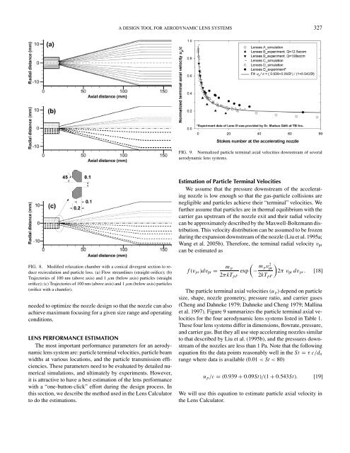
FIG. 8. Modified relaxation chamber with a conical divergent section to reduce recirculation and particle loss. (a) Flow streamlines (straight orifice); (b) Trajectories of 100 nm (above axis) and 1 µm (below axis) particles (straight orifice); (c) Trajectories of 100 nm (above axis) and 1 µm (below axis) particles (orifice with a chamfer). needed to optimize the nozzle design so that the nozzle can also achieve maximum focusing for a given size range and operating conditions. LENS PERFORMANCE ESTIMATION The most important performance parameters for an aerodynamic lens system are: particle terminal velocities, particle beam widths at various locations, and the particle transmission efficiencies. These parameters need to be evaluated by detailed numerical simulations, and ultimately by experiments. However, it is attractive to have a best estimation of the lens performance with a “one-button-click” effort during the design process. In this section, we describe the method used in the Lens Calculator to do the estimations. A DESIGN TOOL FOR AERODYNAMIC LENS SYSTEMS 327 FIG. 9. Normalized particle terminal axial velocities downstream of several aerodynamic lens systems. Estimation of Particle Terminal Velocities We assume that the pressure downstream of the accelerating nozzle is low enough so that the gas-particle collisions are negligible and particles achieve their “terminal” velocities. We further assume that particles are in thermal equilibrium with the carrier gas upstream of the nozzle exit and their radial velocity can be approximately described by the Maxwell-Boltzmann distribution. This velocity distribution can be assumed to be frozen during the expansion downstream of the nozzle (Liu et al. 1995a; Wang et al. 2005b). Therefore, the terminal radial velocity vpr can be estimated as f (vpr)dvpr = m � p exp − 2πkTpF m pv2 � pr 2π vpr dvpr. [18] 2kTpF The particle terminal axial velocities (u p) depend on particle size, shape, nozzle geometry, pressure ratio, and carrier gases (Cheng and Dahneke 1979; Dahneke and Cheng 1979; Mallina et al. 1997). Figure 9 summarizes the particle terminal axial velocities for the four aerodynamic lens systems listed in Table 1. These four lens systems differ in dimensions, flowrate, pressure, and carrier gas. But they all use step accelerating nozzles similar to that described by Liu et al. (1995b), and the pressures downstream of the nozzles are less than 1 Pa. Note that the following equation fits the data points reasonably well in the St = τ c/dn range where data is available (0.01 < St < 80) u p/c = (0.939 + 0.09St)/(1 + 0.543St). [19] We will use this equation to estimate particle axial velocity in the Lens Calculator.
328 X. WANG AND P. H. MCMURRY TABLE 1 Key features of four lens assemblies with step accelerating nozzles used in particle axial velocity comparison Lens system dn (mm) ds (mm) dt (mm) Lt (mm) Gas p1 (Pa) dp (nm) A(Wang et al. 2005b) 2.76 10 6 5 He 528 3–30 B (Liu et al. 1995b) 3.0 10 6 10 Air 93–333 25–250 C (TSI AFL-050) 3.2 17.78 7.62 17.78 Air 250 50–500 D (TSI AFL-100) 1.48 17.78 7.62 17.78 Air 600 100–3000 Estimation of Particle Beam Widths The particle beam width is defined as the beam diameter that encloses 90% of the total particle flux. In this section expressions are given that are used in the Calculator to calculate particle beam widths downstream of each lens as well as downstream of the accelerating nozzle. Bean widths are controlled by two factors: aerodynamic focusing and diffusion broadening. The focusing can be inferred from Figure 2, and the diffusion broadening can be estimated by the root mean square displacement xrms √ = 2Dt, where D is the particle diffusion coefficient, and t is the particle residence time. Assuming the diameters of spacers upstream and downstream of the pressure limiting orifice (lens 0) are the same, the flow is fully developed upstream of the pressure limiting orifice, and particles are homogenously distributed in the flow cross section, the starting particle beam diameter enclosing 90% flux is then ∼0.827ds,0. The particle beam diameter before reaching lens 1 is dB,0 = 0.827ds,0ηc,0 + xrms,0. [20] The beam diameter dB,i at stage i inside the lens system can be easily calculated as dB,i = dB,i−1ηc,i + xrms, i, i = 1ton. [21] However, we should note that dB,i may exceed the spacer diameter ds,i due to defocusing or diffusion. In that case, we assume all particles outside the beam diameter of ds,i are lost and reset dB,i = 0.827 ds,i. Assuming particles achieve a Maxwell-Boltzmann distribution of radial velocities downstream of the acceleration nozzle (lens n + 1), we can estimate the particle beam width at a distance L downstream of the nozzle as follows: dB,n+1 = dB,nηc,n+1 + 3.04 � 2kTpF m p L . [22] Note that ηc,n+1is only a very rough estimate because the pressure downstream of the nozzle is so low that the definition of contraction factor is no longer valid. u p Estimation of Particle Transmission Efficiencies Particle losses in an aerodynamic lens system arise from impaction and diffusion. Particle impaction happens both on the orifice plate and on the spacer walls. We can view the orifices (including the pressure limiting orifice, lenses and the nozzle) as an impactor plate. Particles with large Stokes numbers will fail to follow streamlines and will impact on the plate. Therefore, it is appropriate to use the spacer Stokes number (Sts) tocharacterize particle impaction on the orifice plate. The characteristic velocity and length in Sts are the average flow velocity in the spacer (Us) and the spacer inner diameter (ds), respectively, i.e., Sts = τUs/ds, where Us = 4 Q/(π d2 s ). Figures 10(a)–(c) show the particle transmission efficiency as a function of Sts, Re and Ma for the same conditions as those in Figure 2. The corresponding Stokes numbers based on orifice are also shown in the figures. Note that significant particle losses happen in the Sts range of 0.1–1 for all Reynolds and Mach numbers. Although losses in these figures consist of both losses on the orifice plate and the downstream spacer walls, examination of particle trajectories shows that most losses are due to impaction on the orifice plate for these particular simulations. The transmission curves asymptotically reach ηt = 2( d f ds )2 − ( d f ds )4 for very large Stokes numbers corresponding to geometrical blocking of the orifice plate (Zhang et al. 2002). Figure 11 shows the cutoff Stokes number (Sts50) at which the transmission efficiency is 50% as a function of Re for the three Ma’s studied. From Figure 10 we can see that the impaction particle loss is relatively steep. Therefore, the particle transmission efficiency through the stage from lens i–1 to lens i only considering impaction losses on the orifice plate i, ηt, orifice, i, can be estimated as a step function: ηt, orifice, i = ⎧ ⎪⎨ 1 for Sts < Sts50 or dB,i−1 ≤ d f,i � � d f,i ) 2 � � d 4 f,i 2 d − s,i−1 d . s,i−1 ⎪⎩ �4 for Sts ≥ Sts50 and dB,i−1 > d f,i � � dB,i−1 2 � dB,i−1 2 d − s,i−1 ds,i−1 [23] Note that non-uniform particle concentration due to focusing by upstream lenses is taken into consideration in this equation. Defocused particles will be lost to the wall when ηc < −1. In this case, the initial particle radial position upstream of the
Page 1 and 2: Aerosol Science and Technology, 40:
Page 3 and 4: 322 X. WANG AND P. H. MCMURRY aReyn
Page 5 and 6: 324 X. WANG AND P. H. MCMURRY Furth
Page 7: 326 X. WANG AND P. H. MCMURRY lens
Page 11 and 12: 330 X. WANG AND P. H. MCMURRY DESCR
Page 13 and 14: 332 X. WANG AND P. H. MCMURRY the p
Page 15: 334 X. WANG AND P. H. MCMURRY Gidwa

A Design Tool for Aerodynamic Lens Systems - Department of ...

Create successful ePaper yourself

Delete template?

Save as template?