ANOVA: Advanced Designs
ANOVA: Advanced Designs
ANOVA: Advanced Designs

You also want an ePaper? Increase the reach of your titles
YUMPU automatically turns print PDFs into web optimized ePapers that Google loves.
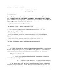
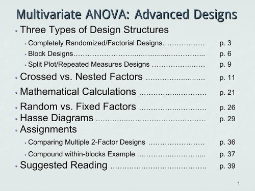
Multivariate <strong>ANOVA</strong>: <strong>Advanced</strong> <strong>Designs</strong><br />
• Three Types of Design Structures<br />
• Completely Randomized/Factorial <strong>Designs</strong>………………<br />
<strong>Designs</strong>………………<br />
p. 3<br />
• Block <strong>Designs</strong>……………………<br />
<strong>Designs</strong>……………………………<br />
………..... .....…… ……………… …………... ... p. 6<br />
• Split Plot/Repeated Measures <strong>Designs</strong> ……………..<br />
……………..……<br />
…… p. 9<br />
• Crossed vs. Nested Factors ……………<br />
• Mathematical Calculations ……………<br />
• Random vs. Fixed Factors ……………<br />
• Hasse Diagrams ………….. …………<br />
Assignments<br />
• Assignments<br />
…………….. ..….. ..…. . p. 11<br />
…………….. ..………… ………… p. 21<br />
…………….. ..………… ………… p. 26<br />
..……………………………<br />
…………………………… p. 29<br />
• Comparing Multiple 2-Factor 2 Factor <strong>Designs</strong> …………………… p. 36<br />
• Compound within-blocks within blocks Example .………… . ………….. ..………… …………... ... p. 37<br />
• Suggested Reading ………………………<br />
……………………….………… …………. p. 39<br />
1
Multivariate <strong>ANOVA</strong>: <strong>Advanced</strong> <strong>Designs</strong><br />
The previous tutorial introduced Analysis of Variance (<strong>ANOVA</strong>) by<br />
discussing one type of design structure, the randomized basic factorial<br />
design. design.<br />
This tutorial will discuss more advanced design structures. To<br />
develop the appropriate <strong>ANOVA</strong> for advanced designs, it is necessary necessary<br />
to<br />
answer the following questions:<br />
1) Is structure of the design:<br />
• a Complete Randomized Design (CR) also called the<br />
Randomized Basic Factorial Design or Factorial Design<br />
• a Block Design, or<br />
• a Split Plot/Repeated Measure (SP/RM) Design?<br />
2) Is each factor crossed or nested? nested<br />
3) Is each factor fixed or random? random<br />
2
Three Types of Design Structures<br />
In Completely Randomized/Factorial <strong>Designs</strong>, <strong>Designs</strong> each condition (specific<br />
combination of factor levels) is randomly assigned to an Experimental<br />
Unit (unit).<br />
Flower Example 1: 1 Students in an introductory statistics class tested the<br />
impact of water solutions on the longevity of cut flowers. They purchased<br />
18 carnations and randomly assigned one of three treatments (plain<br />
water, one aspirin added to the water, and a floral compound provided by<br />
the flower shop) to each flower.<br />
18 units<br />
3 treatments<br />
Plain<br />
Aspirin<br />
Floral Compound<br />
Randomly assign a<br />
treatment to each flower<br />
18 units<br />
Factor: water solution with Levels: plain, aspirin, and floral compound<br />
Unit or EU (experimental unit): each of the 18 flowers<br />
Response: longevity (i.e. number of days until flower starts to wilt)<br />
Null hypothesis: Solution of water makes no difference in the longevity<br />
of carnations.<br />
3
Three Types of Design Structures<br />
This CR design could be analyzed with a 1-factor <strong>ANOVA</strong>, with factor A,<br />
water solution, solution having three levels. An F-statistic would be used to<br />
determine if MSA, the variability between the level means of factor A, is<br />
large compared to the mean square error (MSE), the general flower-toflower<br />
variability. Before this study can extend to the general population of<br />
all carnations, the students need to also address other issues:<br />
1) What care did they take in the experimental process to ensure that<br />
other external factors did not influence the longevity? For example, were<br />
the carnation stems cut at the same time and in the same way? Were the<br />
carnations exposed to the same amount of sunlight, temperature, and<br />
humidity levels?<br />
2) Is their sample truly representative of the the entire population? If their<br />
sample was all the same color or from the same store, it is very likely that<br />
the MSE they calculate from their sample will show less variability than a<br />
true random sample from the entire population. If the MSE is not accurate,<br />
the <strong>ANOVA</strong> is not valid.<br />
In order to draw conclusions from any experiment, it is essential to realize<br />
that the design and procedures are just as important (if not more<br />
important) than any statistical calculations.<br />
4
Three Types of Design Structures<br />
To address these issues, it is important to write very clear procedures<br />
before the experiment begins. For example, since flowers absorb<br />
moisture through the stem, the angle at which a stem is cut is known to<br />
impact flower longevity. Unless cut angle is another variable in their<br />
experimental design, it is important that this potential nuisance variable<br />
is kept as consistent as possible.<br />
These students also chose to restrict their experiment to only white<br />
carnations. Since it is impossible to select a true random sample from<br />
all carnations sold on a particular date, the students had purchased 6<br />
white carnations from three different stores. While not perfect, this is a<br />
very practical approach to account for population variability of white<br />
carnations. Store type clearly was not a factor of interest, but it could<br />
impact the results. Thus it is appropriate to include the nuisance factor,<br />
Store, in the model and analyze the data using a (Randomized) Block<br />
Design instead of a Completely Randomized Design.<br />
5
Three Types of Design Structures<br />
Blocking is the process of grouping units based on some pre-existing<br />
similarity that might impact the results. Units can be sorted, reused, or<br />
subdivided to create a block.<br />
In factorial designs, a treatment is a specific combination of<br />
predetermined factor levels that is assigned to an EU. However, there<br />
are many situations in which a study also includes nuisance factors<br />
(factors that may impact the results but not be of specific interest in the<br />
study). Blocking incorporates nuisance factors into the design in order to<br />
provide more accurate results.<br />
Block effects can be of interest in a study, however since blocks are preexisting<br />
conditions and thus not assigned to EU, there is no causation.<br />
Even without proving causation, blocking is beneficial because it can<br />
increase the efficiency of a design by accounting for some of the model<br />
variability. The Mathematical Calculations section will describe that<br />
including the blocking factor may reduce the experimental error (MSE)<br />
and thus help identify other factors of interest as significant.<br />
6
Three Types of Design Structures<br />
Block <strong>Designs</strong> restrict the way in which the conditions are assigned.<br />
Units are placed into groups (or blocks) of similar units. Units within each<br />
group are assumed to have some similarity that may impact the results.<br />
Within each block, block treatments are randomly assigned to one unit.<br />
Flower Example (continued): The random assignment of treatments to<br />
units was done within each block. Since there are an equal number of<br />
treatments for each store, the effect of water solutions is not biased by<br />
store type. In addition, the students are able to measure the variability<br />
that exists between stores.<br />
Store 1<br />
6 E.U<br />
Store 2<br />
6 E.U<br />
Store 3<br />
6 E.U<br />
3 treatments<br />
Plain<br />
Aspirin<br />
Floral Compound<br />
Within each block (store)<br />
randomly assign a<br />
treatment to each flower<br />
Store 1<br />
6 E.U<br />
Store 2<br />
6 E.U<br />
Store 3<br />
6 E.U<br />
*The Mathematical Calculations section will show that while this is a<br />
block design, the <strong>ANOVA</strong> is identical to a 2-factor <strong>ANOVA</strong> with no<br />
interaction term. One F-test for store effect and another for water solution<br />
effect.<br />
7
Three Types of Design Structures<br />
Before the third design structure is discussed, it is important to understand<br />
the difference between replications and repeated measures. Replications<br />
occur when each condition is assigned to more than one unit.<br />
In the factorial design in Example 1,<br />
each condition had 6 replicates (6<br />
18 E.U<br />
flowers units) that was assigned to<br />
each level of the factor solution. solution<br />
In the block design in Example 1,<br />
each condition had 2 replicates (2<br />
flower units) assigned to each level<br />
within each block. 3 treatments<br />
Store 1<br />
6 E.U<br />
Store 2<br />
6 E.U<br />
Store 3<br />
6 E.U<br />
Plain<br />
Aspirin<br />
Floral Compound<br />
Within each block (store)<br />
randomly assign a<br />
treatment to each flower<br />
3 treatments<br />
Plain<br />
Aspirin<br />
Floral Compound<br />
Randomly assign a<br />
treatment to each flower<br />
Store 1<br />
6 E.U<br />
Store 2<br />
6 E.U<br />
18 E.U<br />
Store 3<br />
6 E.U<br />
Repeated Measures occur when multiple conditions are assigned to one<br />
unit. Thus replications have one measurement for each unit while<br />
repeated measurements have multiple measurements on one unit.<br />
8
Three Types of Design Structures<br />
Split Plot/Repeated Measures <strong>Designs</strong> have at least two sizes of units<br />
in one design. A condition is assigned to a whole plot unit and then the<br />
whole plot unit is reused or subdivided into subgroups (split plot units)<br />
which also receive a condition. The whole plot units act as blocks for the<br />
split plot units.<br />
Popcorn Example 2: 2 To test the effect of storage temperature and<br />
brand on the percentage of popped kernels, a student purchased three<br />
boxes of both an expensive (exp) and generic (gen) popcorn brand.<br />
Each box contained six microwavable bags. Two bags were randomly<br />
selected from each box and stored for one week, one in the refrigerator<br />
(frig) and the other at room (room) temperature. The bags were popped<br />
in random order and the popped and un-popped kernels were counted.<br />
3 Boxes of<br />
Exp Brand Popcorn<br />
3 Boxes of<br />
Gen Brand Popcorn<br />
3 treatments<br />
Refrigerator<br />
Room temperature<br />
Randomly select 2 bags<br />
within each box<br />
3 Boxes of<br />
Exp Brand Popcorn<br />
3 Boxes of<br />
Gen Brand Popcorn<br />
9
Three Types of Design Structures<br />
Whole Plot Factor: brand Whole Plot Unit (Blocks): Box<br />
Split Plot Factor: storage temperature Split Plot Unit: Bag<br />
Response: % popped kernels in a bag<br />
Since boxes were randomly selected from each brand population, the<br />
box-to-box variation should be measured by the experimental error<br />
(whole plot MSE) within brands. brands There are three replicates (three boxes) boxes<br />
for each brand. brand<br />
The popcorn bags within a box are repeated measures (not replicates)<br />
because the bag-to-bag variability with a box is not representative of the<br />
population variability. The bags within each box are likely to be handled<br />
by the same person, at the same time and at the same location. The<br />
bags within a box are considered as sub plot units, because the box<br />
effect is likely to have an impact on the bags selected within the box. box<br />
To test the effect of storage temperature, temp bags were randomly assigned<br />
to a treatment (frig or room) so bags are the appropriate experimental<br />
error (split plot MSE) to measure the temperature temp effect.<br />
10
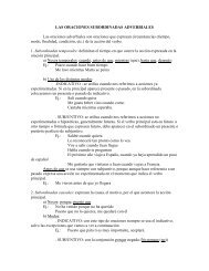
Crossed Vs. Nested Effects<br />
Factors A and B are crossed if every level of A can occur in every level of<br />
B. Factor B is nested in factor A if levels of B only have meaning within<br />
specific levels of A.<br />
In Factorial <strong>Designs</strong>, all factors of interest are crossed and there are no<br />
repeated measures. Block <strong>Designs</strong> can have either crossed or nested<br />
factors. Units are always nested within blocks.<br />
Flower Example (continued): Store and water solution are crossed<br />
factors. Since the same water solution is assigned to flowers from each<br />
store, store the effects of water, aspirin, and floral compound have meaning<br />
across stores and each store effect can also be calculated.<br />
Six flowers (units) are nested within each of the three stores. stores The first<br />
flower purchased from Store 1 is not expected to have any relation to the<br />
first flower purchased from Store 2. So finding a Flower 1 effect across all<br />
three stores is meaningless.<br />
11
Crossed Vs. Nested Effects<br />
Split Plot <strong>Designs</strong> typically have both crossed and nested effects.<br />
Popcorn Example (continued): The whole plot unit (boxes boxes) are nested in<br />
brand. brand The three boxes (B1, B2, B3) appear only under the expensive<br />
level of factor A (brand brand) and the next three boxes (B4, B5, B6) appear only<br />
under the generic level of factor A. In many texts, B4 ,B5, and B6 are also<br />
labeled B1 ,B2, and B3, but it is understood that the B1 occurring in<br />
expensive is different from the B1 occurring in generic.<br />
Bags are nested within boxes. boxes Each bag can only come from one box. box<br />
Storage Temperatures Temp are crossed with brand. brand Each temp [room (T1) and<br />
frig (T2)] occurs in each brand. Since these factors are crossed, room (T1)<br />
is the same under both the expensive and the generic brands.<br />
Storage Temperatures Temp are also crossed with box, box but this interaction effect<br />
is of no interest and typically not shown in an <strong>ANOVA</strong> table.<br />
12
Calculating Crossed Vs. Nested Effects<br />
The calculations for effect size depend on whether a factor is crossed or<br />
nested. These calculations do not depend on whether the factor is a<br />
factor of interest or a nuisance factor.<br />
As shown in the <strong>ANOVA</strong>: Full Factorial Design tutorial, all crossed<br />
effects are calculated by finding the appropriate average and<br />
subtracting the partial fit. All nested effects are also calculated by<br />
finding the appropriate average and subtracting the partial fit. However,<br />
partial fits in nested factors include the factor level in which it is nested.<br />
Flower Example (continued): (continued The effect of “aspirin solution” solution is the<br />
average result of all flowers treated with the aspirin water solution minus<br />
the grand mean. The “store 3” effect is the average result of all flowers<br />
purchased from store 3 minus the grand mean.<br />
Flower (unit) is nested within store. The effect of the 1st flower from<br />
Store1 is calculated:<br />
(average of flower 1 within store1) - (store1 effect + grand mean)<br />
Note that the flower effect is used to calculate MSE. In this study, each<br />
flower is the unit and the average is just the observed result for that single<br />
flower.<br />
13
Calculating Crossed Vs. Nested Effects<br />
Popcorn Example (continued): We can visualize the design structure of<br />
any balanced model with a Hasse (pronounced hahs) diagram. Interaction<br />
terms are listed below the main effects and arrows point from the<br />
interaction to the main effects. Arrows also point from nested factors up to<br />
the factors in which they are nested.<br />
Grand Mean Temperatures Temp and brand are crossed: only<br />
the grand mean is included in their partial fit.<br />
Brand Temp Boxes are nested in brand: brand brand and grand<br />
mean are included in their partial fit.<br />
Box Brand*Temp The brand by temp interaction includes both<br />
brand and temp. temp Thus the partial fit for this<br />
term includes the brand, brand temp and grand<br />
Bag<br />
mean effects.<br />
Bags are nested within boxes (and so also is necessarily nested within<br />
brand). Bags are also randomly selected within temp. temp The partial fit for bag<br />
includes the box, brand, brand*temp, temp and grand mean effects.<br />
Hasse Diagrams will be explained in more detail later in this tutorial. This<br />
example simply is used to visualize the relationship between all factors in<br />
the experiment.<br />
14
Calculating Crossed Vs. Nested Effects<br />
The tables shows a slightly modified data set for the Popcorn Example.<br />
Brand and temp effects are found by subtracting the grand mean from the<br />
appropriate averages.<br />
Brand Box Temp %Popped<br />
exp 1<br />
exp<br />
1<br />
room<br />
frig<br />
84<br />
76<br />
exp 2 room 86<br />
exp 2 frig 86<br />
exp 3 room 91<br />
exp 3 frig 84<br />
gen 1 room 74<br />
gen 1 frig 87<br />
gen 2 room 84<br />
gen 2 frig 83<br />
gen 3 room 83<br />
gen 3 frig 90<br />
Averages<br />
Brand %Popped Temp %Popped<br />
exp 84.5 room 83.67<br />
gen 83.5 frig 84.33<br />
Grand Mean = 84<br />
Main Effects<br />
Brand %Popped Temp %Popped<br />
exp .5 room -.33<br />
gen -.5 frig .33<br />
15
Calculating Crossed Vs. Nested Effects<br />
The Main Effects plot shows that the effect of brand is larger than the<br />
effect of temp. temp In this sample, the expensive brand did better than generic<br />
and refrigerated bags did better than room temperature bags.<br />
Mean of % Popped<br />
84.50<br />
84.25<br />
84.00<br />
83.75<br />
83.50<br />
Main Effects Plot for % Popped<br />
Expensive<br />
Brand Temp<br />
Generic<br />
Frig<br />
Room<br />
Main Effects<br />
Brand %Popped Temp %Popped<br />
exp .5 room -.33<br />
gen -.5 frig .33<br />
Even though the graph<br />
appears to show a<br />
difference between levels,<br />
we do not know at this time<br />
whether these differences<br />
are significant. In other<br />
words, if there really is no<br />
difference in brand, how<br />
often would we expect<br />
effects this large in a<br />
random sample?<br />
16
Calculating Crossed Vs. Nested Effects<br />
The brand by temp interaction is also found with the following formula:<br />
Level average - (brand effect + temp effect + grand mean).<br />
Level<br />
Factor Average<br />
exp room 87<br />
exp frig 82<br />
gen room 80.3333<br />
gen frig 86.6667<br />
Mean<br />
87<br />
86<br />
85<br />
84<br />
83<br />
82<br />
81<br />
80<br />
Interaction Plot for % Popped<br />
Frig<br />
Brand<br />
Effect Temp<br />
Effect Grand<br />
Mean Interaction<br />
Effect<br />
.5 -.333 84 2.83<br />
.5 .333 84 - 2.83<br />
-.5 -.333 84 - 2.83<br />
-.5<br />
.333 84 2.83<br />
Temp<br />
Room<br />
Brand<br />
Expensive<br />
Generic<br />
17
Calculating Crossed Vs. Nested Effects<br />
Referring back to the Hasse diagram, the effects of box and bag factors<br />
still need to be calculated. Since each box only has meaning within a<br />
brand, there are 6 box averages that need to be calculated<br />
Brand Box Temp %Popped<br />
exp 1<br />
exp<br />
1<br />
room<br />
frig<br />
84<br />
76<br />
exp 2 room 86<br />
exp 2 frig 86<br />
exp 3 room 91<br />
exp 3 frig 84<br />
gen 1 room 74<br />
gen 1 frig 87<br />
gen 2 room 84<br />
gen 2 frig 83<br />
gen 3 room 83<br />
gen 3 frig 90<br />
Brand Box<br />
exp<br />
1<br />
Box<br />
Average Brand<br />
effect Grand<br />
Mean<br />
80<br />
.5 84<br />
Box<br />
Effect<br />
-4.5<br />
exp 2 86 .5 84 1.5<br />
exp 3 87.5 .5 84 3<br />
gen 1 80.5 -.5 84 -3<br />
gen 2 83.5 -.5 84 0<br />
gen 3 86.5 -.5 84 3<br />
Crossed effects always sum to zero.<br />
Nested effects (box) also sum to zero<br />
within each appropriate factor level<br />
(brand). Box B1, B2, and B3 effects sum to<br />
zero within the exp brand. Box B1, B2, and<br />
B3 effects sum to zero within the gen<br />
brand.<br />
18
Crossed Vs. Nested Effects<br />
Since bags are the units in this study, the bag effect is the same as a<br />
residual effect. To calculate the residual effect, effect subtract all other effects<br />
from the bag average (observed % popped from each bag).<br />
Brand Box Temp<br />
%<br />
Popped Brand<br />
Effect Temp<br />
Effect Brand*Temp<br />
Effect<br />
Box<br />
Effect<br />
Gran<br />
d<br />
Mean<br />
exp 1 room 84 .5 -.333 2.833 -4.5 84 1.5<br />
exp 1 frig 76 .5 .333 - 2.833 -4.5 84 -1.5<br />
exp 2 room 86 .5 -.333 2.833 1.5 84 -2.5<br />
exp 2 frig 86 .5 .333 - 2.833 1.5 84 2.5<br />
exp 3 room 91 .5 -.333 2.833 3 84 1<br />
Bag<br />
Effect<br />
exp 3 frig 84 .5 .333 - 2.833 3 84 -1<br />
gen 1 room 74 -.5 -.333 - 2.833 -3 84 -3.333<br />
gen 1 frig 87 -.5 .333 2.833 -3 84 3.333<br />
gen 2 room 84 -.5 -.333 - 2.833 0 84 3.667<br />
gen 2 frig 83 -.5 .333 2.833 0 84 -3.667<br />
gen 3 room 83 -.5 -.333 - 2.833 3 84 -0.333<br />
gen 3 frig 90 -.5 .333 2.833 3 84 0.333<br />
Effect sizes still sum to 0<br />
0 0 0 0 0 0<br />
19
Calculating Crossed Vs. Nested Effects<br />
In Summary:<br />
• All effect sizes are calculated by finding the appropriate average and<br />
subtracting the partial fit.<br />
• Partial fits depend on whether a factors are crossed or nested.<br />
• Hasse diagrams are helpful in visualizing complex design structures.<br />
Grand Mean<br />
Brand Temp<br />
Box Brand*Temp<br />
Bag<br />
20
Mathematical Calculations<br />
Effects show the impact of each factor combination and identify which<br />
factors are most influential in our sample. However, a statistical<br />
hypotheses test is needed in order to determine if any of these effects are<br />
significant. Each row corresponding to a factor of interest in the Analysis<br />
of Variance (<strong>ANOVA</strong>) consists of hypothesis tests to determine if there is<br />
statistical evidence that the effects are non-zero.<br />
While effect size calculations vary depending on whether the factor is<br />
crossed or nested, the following calculations are used for all terms in all<br />
balanced designs:<br />
Sum of Squares (SS) = sum of all the squared effects<br />
Degrees of Freedom (df ( df) = number of free units of information<br />
Mean Square (MS) = SS/df for each factor<br />
In SP/RM designs, there are multiple unit sizes and each unit size has an<br />
experimental error (residual) term. The appropriate denominator (MSE) in<br />
the F tests will depend on the three initial questions: 1) design structure, 2)<br />
crossed vs. nested factors, and 3) fixed vs. random factors.<br />
Mean Square Error (MSE) = pooled variance of sample units within each level<br />
F statistic = (MS for each factor)/(appropriate MSE)<br />
21
Mathematical Calculations<br />
Sum of Squares (SS) is calculated by summing the squared factor<br />
SS<br />
=<br />
∑<br />
N<br />
i=<br />
1<br />
( effect)<br />
effect for each run, . For Example 2:<br />
Brand<br />
Effect Temp<br />
Effect<br />
B*T<br />
Effect<br />
.5 -.33 2.83 -4.5<br />
.5<br />
.5<br />
.5<br />
.5<br />
.5<br />
-.5<br />
-.5<br />
-.5<br />
-.5<br />
-.5<br />
-.5<br />
.33<br />
-.33<br />
.33<br />
-.33<br />
.33<br />
-.33<br />
.33<br />
-.33<br />
.33<br />
-.33<br />
.33<br />
- 2.83<br />
2.83<br />
- 2.83<br />
2.83<br />
- 2.83<br />
- 2.84<br />
2.84<br />
- 2.84<br />
2.84<br />
- 2.84<br />
2.84<br />
Box<br />
Effect<br />
-4.5<br />
1.5<br />
1.5<br />
3<br />
3<br />
-3<br />
-3<br />
0<br />
0<br />
3<br />
3<br />
Bag<br />
Effect<br />
1.5<br />
-1.5<br />
-2.5<br />
2.5<br />
1<br />
-1<br />
-3.33<br />
3.33<br />
3.67<br />
-3.67<br />
-0.33<br />
0.33<br />
Sum of Squares<br />
2<br />
Brand<br />
Effect<br />
Squared<br />
Temp<br />
Effect<br />
Squared<br />
B*T<br />
Effect<br />
Squared<br />
0.25 0.11 8.03 20.25<br />
0.25<br />
0.25<br />
0.25<br />
0.25<br />
0.25<br />
0.25<br />
0.25<br />
0.25<br />
0.25<br />
0.11<br />
0.11<br />
0.11<br />
0.11<br />
0.11<br />
0.11<br />
0.11<br />
0.11<br />
0.11<br />
8.03<br />
8.03<br />
8.03<br />
8.03<br />
8.03<br />
8.03<br />
8.03<br />
8.03<br />
8.03<br />
Box<br />
Effect<br />
Squared<br />
20.25<br />
2.25<br />
2.25<br />
9.00<br />
9.00<br />
9.00<br />
9.00<br />
0.00<br />
0.00<br />
Bag<br />
Effect<br />
Squared<br />
2.25<br />
2.25<br />
6.25<br />
6.25<br />
1.00<br />
1.00<br />
11.11<br />
11.11<br />
13.44<br />
13.44<br />
0.25 0.11 8.03 9.00 0.11<br />
0.25 0.11 8.03 9.00 0.11<br />
3.00 1.33 96.33 99.00 68.33<br />
22
Mathematical Calculations<br />
Degrees of Freedom (df ( df) = number of free units of information. In the<br />
popcorn example, there are 2 levels of brand and the <strong>ANOVA</strong><br />
assumptions require that the effects sum to 0. Knowing the effect of the<br />
generic brand automatically forces a known expensive brand effect.<br />
a = # of levels in brand, b = # of levels in temp, c = # of levels of bags within each brand<br />
Brand<br />
Effect Temp<br />
Effect<br />
B*T<br />
Effect<br />
.5 -.33 2.83 -4.5<br />
.5<br />
.5<br />
.5<br />
.5<br />
.5<br />
-.5<br />
-.5<br />
-.5<br />
-.5<br />
-.5<br />
-.5<br />
.33<br />
-.33<br />
.33<br />
-.33<br />
.33<br />
-.33<br />
.33<br />
-.33<br />
.33<br />
-.33<br />
.33<br />
- 2.83<br />
2.83<br />
- 2.83<br />
2.83<br />
- 2.83<br />
- 2.83<br />
2.83<br />
- 2.83<br />
2.83<br />
- 2.83<br />
2.83<br />
Box<br />
Effect<br />
-4.5<br />
1.5<br />
1.5<br />
3<br />
3<br />
-3<br />
-3<br />
0<br />
0<br />
3<br />
3<br />
Bag<br />
Effect<br />
1.5<br />
-1.5<br />
-2.5<br />
2.5<br />
1<br />
-1<br />
-3.33<br />
3.33<br />
3.67<br />
-3.67<br />
-0.33<br />
0.33<br />
For factors not nested in any other factors,<br />
the df is the number of levels minus one.<br />
df Brand = df A = a – 1 = 2-1 = 1<br />
df Temp = df B = b – 1 = 2-1 = 1<br />
For nested factors, factors restrictions in <strong>ANOVA</strong><br />
require that all nested effects sum to zero<br />
within each level of the factor it is nested in.<br />
Box, Box factor C, is nested in brand. brand The three<br />
boxes in the expensive brand need to sum<br />
to 0. If two box effects in expensive are<br />
known, the third box effect is fixed. There<br />
are c-1 pieces of free information for every<br />
level of brand.<br />
dfBox = dfC = a * (c – 1) = 2(3-1) = 4<br />
23
gen<br />
frig<br />
Mathematical Calculations<br />
For the brand*temp (AB) factor interaction, there are a*b effects that are<br />
calculated. Restrictions in <strong>ANOVA</strong> require:<br />
Brand<br />
exp<br />
exp<br />
exp<br />
exp<br />
exp<br />
exp<br />
Temp<br />
room<br />
frig<br />
room<br />
frig<br />
room<br />
frig<br />
Interaction<br />
Effect<br />
2.83<br />
- 2.83<br />
2.83<br />
- 2.83<br />
2.83<br />
- 2.83<br />
1) AB interaction factor effects sum to 0. This requires 1<br />
piece of information to be fixed.<br />
2) The interaction effects within the exp Brand level<br />
sum to 0. The same is true for the gen Brand level. This<br />
requires 1 piece of information to be fixed in each<br />
Brand level. Since 1 value is already used in restriction<br />
1), this requires a-1 pieces of information.<br />
gen<br />
gen<br />
room<br />
frig<br />
- 2.83<br />
2.83<br />
3) The AB effects also sum to 0 within each Temp level.<br />
This requires b-1 pieces of information.<br />
gen room - 2.83 Thus, general rules for a factorial <strong>ANOVA</strong>:<br />
gen<br />
gen<br />
frig<br />
room<br />
2.83<br />
- 2.83<br />
dfBrand*Temp = dfAB = ab – [(a-1) + (b-1) + 1] = (a-1)(b-1)<br />
= 4 – [1+1+1] =1<br />
2.83<br />
Similarly, the df for residuals (bags in our example) also fits these restrictions.<br />
df Bag<br />
= # of effects – [pieces of information already accounted for]<br />
= # of effects – [df Box + df AB + df Brand + df Temp + 1]<br />
= abc – [a(c-1) + (a-1)(b-1) + (a-1) + (b-1) + 1]<br />
= 12 – [2(3-1) + (2-1)*(2-1) + (2-1) + (2-1) +1] = 4<br />
where abc = number of units (bags)<br />
24
Mathematical Calculations<br />
Mean Squares (MS) = SS/df for each factor. MS is a measure of<br />
variability for each factor. Below is the <strong>ANOVA</strong> for Example 2):<br />
Source DF SS MS F P<br />
Brand 1 3.00 3.00 0.12 0.745<br />
Box(Brand)<br />
Box(Brand)<br />
4 99.00 24.75 1.45 0.364<br />
Temp 1 1.33 1.33 0.08 0.794<br />
Brand*Temp 1 96.33 96.33 5.64 0.076<br />
Error 4 68.33 17.08<br />
Total 11 268.00<br />
F-statistic statistic = MS for each factor/MSE. Since there are 2 unit sizes, boxes<br />
and bags, bags there are two error (MSE) terms. The brand F-test uses<br />
box(brand) box(brand [stated box nested within brand] in the denominator. Since<br />
box best represents the variation within brand, it is the whole plot error.<br />
To test the effect of temperature, temp we have two bags that are as similar as<br />
possible (from the same box) and randomly assign a bag to either room<br />
or frig. The F-statistic for temp is MSTemp/MSBag. MSBag is called the split<br />
plot error and is the best measure of variability between bags.<br />
In addition to the design structure and crossed vs. nested factors, each<br />
factor needs to be classified as fixed or random in order to determine<br />
what error term should be used in the denominator for every F-test.<br />
25
Fixed vs. Random Effects<br />
Fixed factors: the levels tested represent all levels of interest<br />
Random factors: the levels tested represent a random sample from<br />
some population of possible levels of interest.<br />
Flower Example (continued): The levels of water solution (plain, aspirin,<br />
and floral compound) are all of specific interest. They are not just a<br />
random selection of all possible items that could be added to water. Thus,<br />
solution is a fixed factor.<br />
The students did not want to compare three specific stores to determine<br />
which store had the best flowers. Instead three stores were randomly<br />
selected from all possible stores to better understand the variability that<br />
exists within the population. Store and flower (units) are random factors.<br />
Popcorn Example (continued): Bags and boxes are random factors.<br />
There were random selections from a population of boxes and a<br />
population of bags. Brand and temp are fixed factors. If we were not<br />
interested in finding the effect of expensive and generic brands, but<br />
instead simply randomly selected two solutions of brands from all possible<br />
brands, then brand would be a random factor. Determination of whether<br />
effects are fixed or random can vary, and the choice can greatly impact<br />
the <strong>ANOVA</strong> analysis.<br />
26
Fixed vs. Random Effects<br />
Fixed factors have meaning only at the levels that were included in the<br />
experimental design. The same levels of that factor would be used if<br />
the experiment was repeated.<br />
Since the levels of random factors were randomly selected, the results<br />
have meaning for the levels selected in the study as well as any levels<br />
not included in the study. Different levels would be randomly selected if<br />
the experiment was repeated. Blocks and units are typically classified<br />
as random effects.<br />
Now that the key questions have been answered:<br />
1) Is structure of the design:<br />
• a Complete Randomized Design/Factorial Design<br />
• a Block Design, or<br />
• a Split Plot/Repeated Measure Design?<br />
2) Is each factor is crossed or nested?<br />
3) Is each factor is fixed or random?<br />
Hasse diagrams can be used to determine what error term should be<br />
used in the denominator for every F test. Hasse diagrams are effective<br />
for all balanced designs (i.e. same number of units in every condition).<br />
27
Rules for Developing Hasse Diagrams<br />
1) Start row 1 with node M for the grand mean<br />
2) Put a node on row 2 for each factor that is not nested in any term. Add arrows<br />
from each node on row 2 to the grand mean. Place parentheses around any<br />
random factor.<br />
3) Add a node on row 3 for any factor nested in row 2, and draw arrows to the<br />
row 2 nodes. Add a node for any 2-way interaction and draw arrows to the<br />
individual factors in row 2. Place parentheses around any random factor or<br />
any factor that is nested in a random factor. If an interaction term contains at<br />
least 1 random effect, the entire interaction is considered random.<br />
4) On each successive row, say row “i”, add a node for any factor nesting in row<br />
“i-1”. Add a node for any “i-way interaction”. Draw appropriate arrows to the “i-<br />
1” nodes and place parentheses around any random factor or any factor that<br />
is nested in a random factor.<br />
5) When all interactions or nested factors are exhausted, add a node for error on<br />
the bottom line, and draw arrows to nodes in the row above.<br />
6) For each node, add a superscript that indicates the number of effects for each<br />
term (# of interaction effects are always products of the # of main effects).<br />
7) For each node, add a subscript that indicates the degrees of freedom for that<br />
term. Degrees of freedom for a term are found by starting with the superscript<br />
for that particular node and subtracting out the degrees of freedom for all<br />
terms connected with arrows above it.<br />
28
Mathematical Calculations: Hasse Diagram<br />
If the Hasse Diagram is developed, the denominator for the appropriate<br />
F test is typically straightforward:<br />
The denominator for testing node A is the next eligible random term term<br />
below A in the Hasse diagram.<br />
If there are 2 or more “next eligible random terms” then use an<br />
approximate test. test Approximate tests usually are a combination of<br />
existing MS values. Most software packages do this automatically.<br />
In more complex models that include mixed interaction terms (there<br />
are both fixed and random factors in the interaction), it is necessary to<br />
determine whether the effects are Restricted or Unrestricted. In<br />
general, restricted effects sum to zero while unrestricted effects do not.<br />
However, this classification tends to be rather complex and the analysis<br />
is best done with a statistician. Texts listed at the end of this tutorial all<br />
discuss restricted and unrestricted effects in more detail.<br />
29
Mathematical Calculations<br />
Hasse Diagram for the Flower Example; Example<br />
Store 1<br />
6 E.U<br />
Grand Mean<br />
Store 2<br />
6 E.U<br />
(Store) Solution<br />
(Flower)<br />
Store 3<br />
6 E.U<br />
3 treatments<br />
Plain<br />
Aspirin<br />
Floral Compound<br />
Within each block (store)<br />
randomly assign a<br />
treatment to each flower<br />
Store 1<br />
6 E.U<br />
Store 2<br />
6 E.U<br />
Store 3<br />
6 E.U<br />
1) Start row 1 with a node for the grand mean<br />
2) Put a node on row 2 for each factor that is not<br />
nested in any term. Add arrows from each<br />
node on row 2 to the grand mean. Place<br />
parentheses around any random factor.<br />
3) Add a node on row 3 for any factor nested in<br />
row 2, and draw arrows to the row 2 nodes.<br />
Place parentheses around any random factor<br />
or any factor that is nested in a random factor.<br />
No 2-factor interactions are used.<br />
4) No successive rows needed.<br />
30
Mathematical Calculations<br />
Hasse Diagram for the Flower Example (continued):<br />
Grand Mean 1 1<br />
(Store) 3 2 Solution 3 2<br />
(Error) 18 13<br />
Flowers are the units,<br />
thus the flower effect is<br />
identical to the residual<br />
effect (i.e. the error term).<br />
5) When all interactions or nested factors are<br />
exhausted, add a node for error on the bottom line,<br />
and draw arrows to nodes in the row above.<br />
6) For each node, add a superscript that indicates the<br />
number of levels for each term. (# of interaction<br />
effects are always products of the # of main effects)<br />
7) For each node, add a subscript that indicates the<br />
degrees of freedom for that term. Degrees of<br />
freedom for a term are found by starting with the<br />
superscript for that particular node and subtracting<br />
out the degrees of freedom for all terms connected<br />
with arrows above it (i.e. subtracting df from all<br />
terms included in the partial fit).<br />
For this study, there is only one error term (thus only one MSE). Error is<br />
the first random term following the store effect and the water solution<br />
effect. Thus error (i.e. flower or unit) is the denominator in both F-tests.<br />
31
Mathematical Calculations<br />
The correct <strong>ANOVA</strong> for the Flower Example:<br />
Source df SS MS F P<br />
Store 2 13 6.5 8.05 0.005<br />
Solution 2 9 4.5 5.57 0.018<br />
Error 13 10.5 0.8<br />
Total 17 32.5<br />
solution<br />
Store 1<br />
days<br />
Store 2<br />
days<br />
Store 3<br />
days<br />
water 7 6 6<br />
water 9 7 5<br />
aspirin 6 6 4<br />
aspirin 5 5 5<br />
compound 8 7 6<br />
compound 7 8 4<br />
Note that if the students had ignored the store effect. The <strong>ANOVA</strong> would<br />
look like:<br />
Source df SS MS F P<br />
Note that the solution df and SS are<br />
identical in both <strong>ANOVA</strong>s. However,<br />
Solution 2 9.0 4.50 2.87 0.088 the error term in the 2<br />
Error 15 23.5 1.57<br />
Total 17 32.5<br />
nd <strong>ANOVA</strong><br />
combines the store and the flower<br />
(error error) effects.<br />
If store variability is ignored (just assumed to be flower-to-flower<br />
variability), it overshadows the effects of solution, solution and the students<br />
would incorrectly conclude that solution is not significant.<br />
Students could have decided to eliminate store variability by only buying<br />
flowers from Store 1. However, then conclusions from this study could<br />
only extend to carnations purchased from that particular store.<br />
32
Mathematical Calculations<br />
Hasse Diagram for Popcorn Example: Example<br />
1) Start row 1 with a node for the grand mean<br />
2) Put a node on row 2 for each factor that is not<br />
Grand Mean<br />
nested in any term. Add arrows from each node on<br />
row 2 to the grand mean.<br />
Brand Temp 3) Add a node on row 3 for any factor nested in row 2,<br />
and draw arrows to the appropriate row 2 nodes.<br />
Add a node for any 2-way interaction and draw<br />
(Box) Brand*Temp arrows to the individual factors in row 2. Place<br />
parentheses around any random factor or any<br />
factor that is nested in a random factor. If an<br />
(Bag)<br />
interaction term contains at least 1 random effect,<br />
the entire interaction is considered random.<br />
4) On each successive row, say row “i”, add a node<br />
for any factor nesting in row “i-1”. Add a node for<br />
any “i-way interaction”. Draw appropriate arrows to<br />
the “i-1” nodes and place parentheses around any<br />
random factor or any factor that is nested in a<br />
random factor.<br />
33
Mathematical Calculations<br />
Hasse Diagram for Popcorn Example (continued):<br />
Grand Mean1 1<br />
Brand2 1 Temp2 1<br />
(Box) 6 4 Brand*Temp4 (Error) 12 5) When all interactions or nested factors are<br />
exhausted, add a node for error on the bottom<br />
line, and draw arrows to nodes in the row above.<br />
6) For each node, add a superscript that indicates<br />
the number of levels for each term. (# of<br />
interaction effects are always products of the #<br />
1<br />
of main effects)<br />
7) For each node, add a subscript that indicates<br />
the degrees of freedom for that term. Degrees of<br />
4<br />
freedom for a term are found by starting with the<br />
superscript for that particular node and<br />
subtracting out the degrees of freedom for all<br />
terms connected with arrows above it.<br />
For this study, box (whole plot error) is the first random term below brand<br />
and thus is used in the denominator for the brand F-test.<br />
Bag (error or sub plot error) is the first random term below temp and<br />
brand*temp, brand*temp thus error (i.e. bag or split plot unit) is the denominator in<br />
both temp and brand*temp F-tests.<br />
34
Grand Mean 1 1<br />
(Store) 3 2 Solution3 2<br />
(Error) 18 13<br />
Mathematical Calculations<br />
Comparison of the Flower and Popcorn Examples:<br />
Store 1<br />
6 units<br />
Store 2<br />
6 units<br />
Store 3<br />
6 units<br />
Grand Mean 1 1<br />
Brand 2 1<br />
Temp 2 1<br />
(Box) 6 4 Brand*Temp4 1<br />
(Error) 12 4<br />
3 Boxes of<br />
Exp Brand Popcorn<br />
3 Boxes of<br />
Gen Brand Popcorn<br />
Both the Flower and Popcorn Examples have units assigned within larger<br />
groups (flowers within stores and boxes within brand). The key difference<br />
between Block designs and SP/RM designs are the units. In the Flower<br />
Example, only one measurement (longevity) is taken on each unit. SP/RM<br />
designs take more than one measurement on the same unit (2 bags were<br />
measured within each box). Thus the Popcorn SP/RM Example has two<br />
sizes of units (boxes – the whole plot unit and bag-the split plot unit).<br />
While graphics are very useful in determining what condition is applied to<br />
each unit, the Hasse diagram can also identify whether the factors are<br />
crossed/nested or fixed/random.<br />
35
Assignment<br />
Comparison of 2 factor models: models Remember that df, SS and MS depend<br />
upon 1) the design structure and 2) whether the factors are crossed or<br />
nested. Also, F-ratios cannot be calculated unless you also know 3)<br />
whether factors are fixed or random. The following table shows data<br />
from an experiment with 2 factors, A and B. For each of the four<br />
situations, use the same data to create Hasse diagrams and <strong>ANOVA</strong><br />
tables.<br />
trial A B Results<br />
1 a1 b1 80<br />
2 a1 b1 70<br />
3 a2 b1 30<br />
4 a2 b1 36<br />
5 a3 b1 46<br />
6 a3 b1 38<br />
7 a1 b2 46<br />
8 a1 b2 44<br />
9 a2 b2 16<br />
10 a2 b2 18<br />
11 a3 b2 32<br />
12 a3 b2 24<br />
1) A and B crossed [written A x B or AB], any combination<br />
of fixed and random effects.<br />
2) A nested in B [this is written A(B)], A fixed B fixed<br />
3) A nested in B [this is written A(B)], A random B fixed<br />
4) A nested in B [this is written A(B)], A random B random<br />
*It typically doesn’t make sense to have a fixed factor<br />
nested within a random factor. For example, if you<br />
randomly select 10 trees, factor B, and then choose 5<br />
leaves nested within each tree, factor A, it is reasonable<br />
to assume that since trees are random, so are the<br />
leaves.<br />
36
Assignment<br />
Two students designed an experiment to test for the effects of several factors on<br />
memorization. 13 students were selected from 4 majors (52 students total). Each<br />
student was asked to read 4 lists of 20 words, (ABS/M, ABS/E, CONC/M, and<br />
CONC/E), in random order.<br />
Three Factors of interest:<br />
• Major, Major 4 levels: Mathematics, Computer Science, History, and English<br />
• List-Type List Type, 2 levels: Abstract Words (harder to remember) and Concrete Words<br />
• Distraction-Type<br />
Distraction Type, 2 levels: Math [Count down from 262 by 3’s for 30 seconds] and<br />
English [read Robert Frost’s The Road Less Traveled and describe the theme of the poem]<br />
Nuisance Factor: Student 6 students were randomly selected from each major.<br />
Response: Response number of words a student could recall.<br />
List, Distraction form a 2-way factorial design within each student, this is called a<br />
compound within-blocks treatment with students as the block/whole plot unit.<br />
There are a total of 96 split plot units [4 majors*6 students*2 list-types*2<br />
distractions]. Each list of 20 words is a split plot unit used to test the effect of<br />
List-Type and Distraction.<br />
37
Assignment<br />
Create a Hasse Diagram for this study and complete the following<br />
<strong>ANOVA</strong>.<br />
Source df SS MS F P<br />
Major 40.792 .314<br />
Subject(Major) 215.167 .003<br />
Distraction 5.042 .277<br />
List-Type 112.667 .000<br />
Distraction*List-Type 0.667 .691<br />
Major*Distraction 41.125<br />
Major*List-Type 9.000<br />
Major*Distraction*List-Type 13.000<br />
Error 251.500<br />
Total 688.958<br />
38
Suggested Reading<br />
Hunter, W. G., “Some Some Ideas about Teaching and Design of Experiments, with<br />
2^5 Examples of Experiments Conducted by Students”, Students , The American<br />
Statistician, Vol. 31, No. 1 (Feb., 1977), 12-17. 12 17.<br />
Suggested Textbooks<br />
Design and Analysis of Experiments by George Cobb,<br />
Prerequisites: none<br />
Examples: wide variety<br />
Design and Analysis of Experiments by Gary Oehlert,<br />
Prerequisites: prior statistics courses are beneficial<br />
Examples: primarily from science and engineering<br />
Design and Analysis of Experiments by David Montgomery,<br />
Prerequisites: prior statistics courses are beneficial<br />
Examples: primarily engineering<br />
39
Suggested Reading<br />
The Hasse diagram provides a visual display of the relationships between<br />
factors for balanced complete experimental designs. Using the Hasse diagram,<br />
rules exist for determining the appropriate linear model, <strong>ANOVA</strong> table,<br />
expected means squares, and F-tests.<br />
Iverson, P.W. and Marasinghe, M.G.(2005). Visualizing Experimental <strong>Designs</strong> for<br />
Balanced <strong>ANOVA</strong> Models Using Lisp-Stat. Journal of Statistical Software, 18, 3.<br />
http://www.jstatsoft.org/v13/i03/v13i03.pdf<br />
Kempthorne, O. (1982). Classificatory Data Structures and Associated Linear Models, in<br />
Essays in Honor of C. R. Rao, G. Killianpur, P. R. Krishnaiah, J. K. Ghosh,eds. New<br />
York: North Holland, 397-410.<br />
Lohr, S. L. (1995). Hasse Diagrams in Statistical Consulting and Teaching. The American<br />
Statistician, 49, 4, 376-381.<br />
Marasinghe, M. G. and Darius P. L. (1990). A Structure-Based Approach for Model<br />
Determination in Experimental <strong>Designs</strong>. Proc. Stat. Comp. Section, American Statistical<br />
Association, 143-150.<br />
Oehlert, Oehlert,<br />
G., “A A First Course in Design and Analysis of Experiments”, Experiments , Freeman<br />
Publishers, 2000<br />
Searle, S. R. (1971). Linear Models. New York: Wiley.<br />
Taylor, W. H. and Hilton, H. G. (1981). A Structure Diagram Symbolization for Analysis of<br />
Variance. The American Statistican, 35, 2, 85-93.<br />
40
Additional Terminology<br />
The following are additional terms and techniques that can be used in<br />
developing advanced <strong>ANOVA</strong> models. While many of these are beyond<br />
the scope of this tutorial, they are all discussed in more detail in the<br />
suggested textbooks.<br />
Often factors or designs are described based on their relationship to units.<br />
When units are nested within factors, they are called between group<br />
factors. factors<br />
If some combination of factors are allocated within units, they are called<br />
within group factors. factors<br />
Latin Square <strong>Designs</strong> are designs with two blocking factors (two<br />
nuisance factors) and one factor of interest.<br />
Nested designs are also called hierarchical designs<br />
hierarchical designs. These designs can<br />
have 3 or more levels of nesting. For example, trees could be nested<br />
within fields and leaves nested in trees.<br />
41