Runge-Kutta Method - Clarkson University

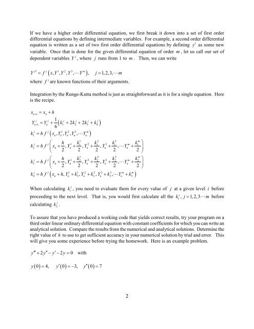
If we have a higher order differential equation, we first break it down into a set of first order
differential equations by defining intermediate variables. For example, a second order differential
equation is written as a set of two first order differential equations by defining y′ as some new
variable. Once that is done for the given differential equation of order m , let us call our set of
j
dependent variables Y , where j runs from 1 to m . Then, we can write
1 2 3 ( )
j j m
Y′ = f xY , , Y , Y , �Y, j= 1, 2, 3, �m
where
j
f are known functions of their arguments.
Integration by the Runge-Kutta method is just as straightforward as it is for a single equation. Here
is the recipe.
xn+ 1 xn h = +
Yn+ Yn 1
6
k 2k 2k
k
= + + + +
j j
k1 = hf
1 2 3 m
xn, Yn, Yn , Yn , � Yn
( )
( )
j j j j j j
1 1 2 3 4
1 2 3
m
j j⎛ h 1 k1 2 k1 3 k1 m k ⎞ 1
k2 = hf ⎜xn + , Yn + , Yn + , Yn + , � Yn
+ ⎟
⎝ 2 2 2 2 2 ⎠
1 2 3
m
j j⎛ h 1 k2 2 k2 3 k2 m k ⎞ 2
k3 = hf ⎜xn + , Yn + , Yn + , Yn + , � Yn
+ ⎟
⎝ 2 2 2 2 2 ⎠
j j 1 1 2 2 3 3 m m
k = hf x + hY , + k, Y + k , Y + k , � Y + k
( n n n n n )
4 3 3 3 3
j
When calculating k i , you need to evaluate them for every value of j at a given level i before
j
proceeding to the next level. That is, you would first calculate all the k1 , j = 1, 2, 3�
m before
j
calculating k 2 .
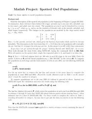
To assure that you have produced a working code that yields correct results, try your program on a
third order linear ordinary differential equation with constant coefficients for which you can write an
analytical solution. Compare the results from the numerical and analytical solutions. Determine the
right value of h to use to get sufficient accuracy in your numerical solution by trial and error. This
will give you some experience before trying the homework. Here is an example problem.
y′′′ + 2y′′ − y′ − 2y = 0 with
( ) ′ ( ) ′′ ( )
y 0 = 4, y 0 =− 3, y 0 =
7
2