Runge-Kutta Method - Clarkson University
Runge-Kutta Method - Clarkson University
Runge-Kutta Method - Clarkson University

Create successful ePaper yourself
Turn your PDF publications into a flip-book with our unique Google optimized e-Paper software.
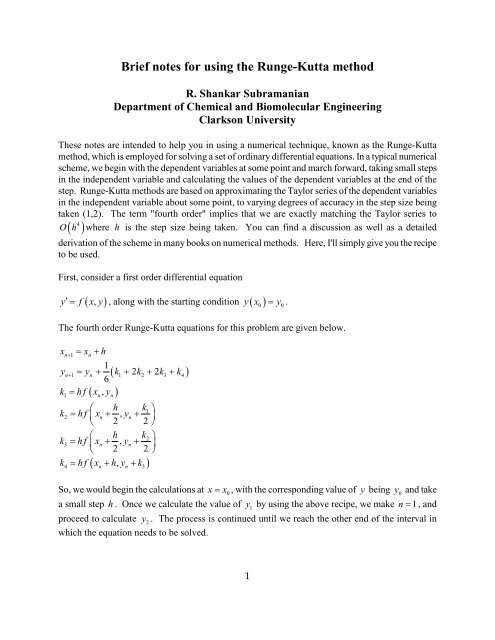
Brief notes for using the <strong>Runge</strong>-<strong>Kutta</strong> method<br />
R. Shankar Subramanian<br />
Department of Chemical and Biomolecular Engineering<br />
<strong>Clarkson</strong> <strong>University</strong><br />
These notes are intended to help you in using a numerical technique, known as the <strong>Runge</strong>-<strong>Kutta</strong><br />
method, which is employed for solving a set of ordinary differential equations. In a typical numerical<br />
scheme, we begin with the dependent variables at some point and march forward, taking small steps<br />
in the independent variable and calculating the values of the dependent variables at the end of the<br />
step. <strong>Runge</strong>-<strong>Kutta</strong> methods are based on approximating the Taylor series of the dependent variables<br />
in the independent variable about some point, to varying degrees of accuracy in the step size being<br />
taken (1,2). The term "fourth order" implies that we are exactly matching the Taylor series to<br />
4<br />
O( h ) where h is the step size being taken. You can find a discussion as well as a detailed<br />
derivation of the scheme in many books on numerical methods. Here, I'll simply give you the recipe<br />
to be used.<br />
First, consider a first order differential equation<br />
′ = ( , ) , along with the starting condition ( )<br />
y f xy<br />
y x = y .<br />
1<br />
0 0<br />
The fourth order <strong>Runge</strong>-<strong>Kutta</strong> equations for this problem are given below.<br />
xn+ 1 xn h = +<br />
1<br />
yn+ yn k 2k 2k<br />
k<br />
6<br />
= + + + +<br />
k1 = hf ( xn, yn)<br />
⎛ h k1<br />
⎞<br />
k2 = hf ⎜xn + , yn<br />
+ ⎟<br />
⎝ 2 2 ⎠<br />
⎛ h k2<br />
⎞<br />
k3 = hf ⎜xn + , yn<br />
+ ⎟<br />
⎝ 2 2 ⎠<br />
k = hf x + h, y + k<br />
( )<br />
1 1 2 3 4<br />
( )<br />
4 n n 3<br />
So, we would begin the calculations at x= x0,<br />
with the corresponding value of y being y 0 and take<br />
a small step h . Once we calculate the value of y 1 by using the above recipe, we make n = 1,<br />
and<br />
proceed to calculate y 2 . The process is continued until we reach the other end of the interval in<br />
which the equation needs to be solved.
If we have a higher order differential equation, we first break it down into a set of first order<br />
differential equations by defining intermediate variables. For example, a second order differential<br />
equation is written as a set of two first order differential equations by defining y′ as some new<br />
variable. Once that is done for the given differential equation of order m , let us call our set of<br />
j<br />
dependent variables Y , where j runs from 1 to m . Then, we can write<br />
1 2 3 ( )<br />
j j m<br />
Y′ = f xY , , Y , Y , �Y, j= 1, 2, 3, �m<br />
where<br />
j<br />
f are known functions of their arguments.<br />
Integration by the <strong>Runge</strong>-<strong>Kutta</strong> method is just as straightforward as it is for a single equation. Here<br />
is the recipe.<br />
xn+ 1 xn h = +<br />
Yn+ Yn 1<br />
6<br />
k 2k 2k<br />
k<br />
= + + + +<br />
j j<br />
k1 = hf<br />
1 2 3 m<br />
xn, Yn, Yn , Yn , � Yn<br />
( )<br />
( )<br />
j j j j j j<br />
1 1 2 3 4<br />
1 2 3<br />
m<br />
j j⎛ h 1 k1 2 k1 3 k1 m k ⎞ 1<br />
k2 = hf ⎜xn + , Yn + , Yn + , Yn + , � Yn<br />
+ ⎟<br />
⎝ 2 2 2 2 2 ⎠<br />
1 2 3<br />
m<br />
j j⎛ h 1 k2 2 k2 3 k2 m k ⎞ 2<br />
k3 = hf ⎜xn + , Yn + , Yn + , Yn + , � Yn<br />
+ ⎟<br />
⎝ 2 2 2 2 2 ⎠<br />
j j 1 1 2 2 3 3 m m<br />
k = hf x + hY , + k, Y + k , Y + k , � Y + k<br />
( n n n n n )<br />
4 3 3 3 3<br />
j<br />
When calculating k i , you need to evaluate them for every value of j at a given level i before<br />
j<br />
proceeding to the next level. That is, you would first calculate all the k1 , j = 1, 2, 3�<br />
m before<br />
j<br />
calculating k 2 .<br />
To assure that you have produced a working code that yields correct results, try your program on a<br />
third order linear ordinary differential equation with constant coefficients for which you can write an<br />
analytical solution. Compare the results from the numerical and analytical solutions. Determine the<br />
right value of h to use to get sufficient accuracy in your numerical solution by trial and error. This<br />
will give you some experience before trying the homework. Here is an example problem.<br />
y′′′ + 2y′′ − y′ − 2y = 0 with<br />
( ) ′ ( ) ′′ ( )<br />
y 0 = 4, y 0 =− 3, y 0 =<br />
7<br />
2
The analytical solution is<br />
y = e + 2e<br />
+ e<br />
x −x −2x<br />
References<br />
1. F.B. Hildebrand, Advanced Calculus for Applications, Prentice-Hall, New Jersey 1976.<br />
2. W.H. Press, S.A. Teukolsky, W.T. Vetterling, and B.P. Flannery, Numerical Recipes in<br />
FORTRAN, Cambridge <strong>University</strong> Press, Cambridge, UK, 1992.<br />
3