Reflectance Model for Diffraction - EDM - UHasselt
Reflectance Model for Diffraction - EDM - UHasselt
Reflectance Model for Diffraction - EDM - UHasselt

You also want an ePaper? Increase the reach of your titles
YUMPU automatically turns print PDFs into web optimized ePapers that Google loves.
<strong>Reflectance</strong> <strong>Model</strong> <strong>for</strong> <strong>Diffraction</strong><br />
TOM CUYPERS and TOM HABER and PHILIPPE BEKAERT<br />
Hasselt University - tUL - IBBT<br />
Expertise Centre <strong>for</strong> Digital Media, Belgium<br />
and<br />
SE BAEK OH<br />
MIT: Mechanical Engineering<br />
and<br />
RAMESH RASKAR<br />
MIT MediaLab: Camera Culture<br />
We present a novel method of simulating wave effects in graphics using<br />
ray–based renderers with a new function: the Wave BSDF (Bidirectional<br />
Scattering Distribution Function). Reflections from neighboring surface<br />
patches represented by local BSDFs are mutually independent. However,<br />
in many surfaces with wavelength–scale microstructures, interference and<br />
diffraction requires a joint analysis of reflected wavefronts from neighboring<br />
patches. We demonstrate a simple method to compute the BSDF <strong>for</strong><br />
the entire microstructure, which can be used independently <strong>for</strong> each patch.<br />
This allows us to use traditional ray–based rendering pipelines to synthesize<br />
wave effects. We exploit the Wigner Distribution Function (WDF) to<br />
create transmissive, reflective, and emissive BSDFs <strong>for</strong> various diffraction<br />
phenomena in a physically accurate way. In contrast to previous methods<br />
<strong>for</strong> computing interference, we circumvent the need to explicitly keep track<br />
of the phase of the wave by using BSDFs that include positive as well as<br />
negative coefficients. We describe and compare the theory in relation to<br />
well understood concepts in rendering and demonstrate a straight<strong>for</strong>ward<br />
implementation. In conjunction with standard raytracers, such as PBRT, we<br />
demonstrate wave effects <strong>for</strong> a range of scenarios such as multi–bounce<br />
diffraction materials, holograms and reflection of high frequency surfaces.<br />
Categories and Subject Descriptors: I.3.5 [Computer Graphics]: Computational<br />
Geometry and Object <strong>Model</strong>ing—Physically based modeling<br />
General Terms: Simulating Natural Phenomena<br />
Additional Key Words and Phrases: <strong>Diffraction</strong>, Interference, Wave Effects,<br />
Wigner Distribution Function, Wave Optics<br />
ACM Reference Format:<br />
Authors’ addresses: tom.cuypers@uhasselt.be, tom.haber@uhasselt.be,<br />
philippe.bekaert@uhasselt.be, sboh@alum.mit.edu,<br />
raskar@media.mit.edu.<br />
Permission to make digital or hard copies of part or all of this work <strong>for</strong><br />
personal or classroom use is granted without fee provided that copies are<br />
not made or distributed <strong>for</strong> profit or commercial advantage and that copies<br />
show this notice on the first page or initial screen of a display along with<br />
the full citation. Copyrights <strong>for</strong> components of this work owned by others<br />
than ACM must be honored. Abstracting with credit is permitted. To copy<br />
otherwise, to republish, to post on servers, to redistribute to lists, or to use<br />
any component of this work in other works requires prior specific permission<br />
and/or a fee. Permissions may be requested from Publications Dept.,<br />
ACM, Inc., 2 Penn Plaza, Suite 701, New York, NY 10121-0701 USA, fax<br />
+1 (212) 869-0481, or permissions@acm.org.<br />
c○ 2009 ACM 0730-0301/2009/12-ART106 $10.00<br />
DOI 10.1145/1559755.1559763<br />
http://doi.acm.org/10.1145/1559755.1559763<br />
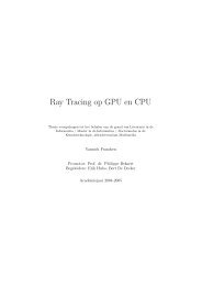
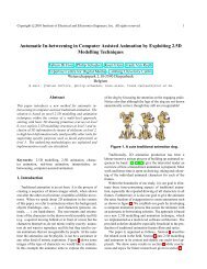
Fig. 1: We generalize the rendering equation and the BSDF to simulate wave<br />
phenomena. The new Wave BSDF behaves like a local scattering function,<br />
creates interference globally, and allows easy integration into traditional ray<br />
based methods.<br />
Cuypers, T., Oh, S.B., Haber, T., Bekaert, P., Raskar, R. <strong>Reflectance</strong> <strong>Model</strong><br />
<strong>for</strong> <strong>Diffraction</strong>. TODO<br />
1. INTRODUCTION<br />
<strong>Diffraction</strong> is a common phenomenon in nature when dealing with<br />
small scale occluders. It can be observed on animals, such as feathers<br />
and butterfly wings, and man-made objects like rainbow holograms.<br />
In acoustics, the effect of diffraction is even more significant<br />
due to the much longer wavelength of sound. In order to simulate<br />
effects such as interference and diffraction within a ray based<br />
framework, the phase of light needs to be integrated into those<br />
methods.<br />
We introduce a novel method <strong>for</strong> creating Bidirectional Scattering<br />
Distribution Functions (BSDFs), which efficiently simulate<br />
diffraction and interference in ray-based frameworks. The reflected<br />
or scattered radiance of a ray indirectly and independently encodes<br />
the mutual phase in<strong>for</strong>mation among the rays, conveniently allow-<br />
ACM Transactions on Graphics, Vol. 28, No. 4, Article 106, Publication date: August 2009.
2 • T. Cuypers et al.<br />
Strategy Create new wavefronts<br />
with phase computation<br />
Sample papers Moravec1981<br />
Ziegler2008<br />
Effects<br />
OPD: Phase Tracking <strong>Diffraction</strong> Shaders Augmented Lightfields<br />
(ALF)<br />
Instantaneous diffraction<br />
and interference<br />
Stam1999<br />
Lindsay2006<br />
Two plane lightfield<br />
parameterization<br />
Edge <strong>Diffraction</strong> Our Technique<br />
Edge-only diffraction,<br />
OPD <strong>for</strong> interference<br />
Oh2010 Freniere1999<br />
Tsingos2000<br />
<strong>Diffraction</strong> Yes Yes Yes Yes (at edges) Yes<br />
Interference At receiver Single point-single<br />
direction<br />
BRDF with negative<br />
radiance coefficients<br />
At receiver At receiver At receiver<br />
Near vs. far field Both Far field Both Near field: approx. (GTD),<br />
Far field accurate<br />
Global illumination Yes Possible in far field, not<br />
shown<br />
Transmission / reflection<br />
/ absorption<br />
All Reflection shown ,<br />
Transmission possible (*)<br />
Both<br />
No Yes Yes<br />
Transmission only Transmission and<br />
Reflection<br />
Emissive elements Yes Not shown Possible, not shown Not applicable Yes<br />
Phase vs. amplitude<br />
grating<br />
Both Phase shown,<br />
Amplitude possible (*)<br />
Light vs. Audio Both Light shown,<br />
Audio possible in far field<br />
Implementation<br />
Amplitude shown,<br />
Phase possible<br />
Light shown,<br />
Audio possible<br />
All<br />
Both Both<br />
Typically <strong>for</strong> audio Both<br />
(Appendix B)<br />
Convenience -- ++ + - ++<br />
Explicit phase<br />
representation<br />
Yes Not required Not required Yes Not required<br />
Speed: direct illumination + +++++ - +++ +++++<br />
Speed: global illumination -- N/A N/A ++ ++<br />
Importance Sampling No N/A No Implicit Yes<br />
Scatter / gather<br />
operations<br />
Statistical vs. explicit<br />
micro geometry<br />
Scenarios demonstrating<br />
limitations<br />
Deferred diffraction and<br />
interference<br />
Instantaneous diffraction<br />
and interference<br />
Deferred diffraction and<br />
interference<br />
Deferred diffraction and<br />
interference<br />
Explicit only Both Explicit only Explicit only Both<br />
Sinusoidal grating,<br />
Speaker array<br />
Lens + aperture,<br />
Audio rendering<br />
2 CDs <strong>Diffraction</strong> from sliding<br />
door<br />
Instantaneous diffraction,<br />
deferred interference<br />
Less accurate outside<br />
paraxial zone<br />
(*) Section 5.2 shows our suggestions <strong>for</strong> improvements<br />
Table I. : Overview of different rendering strategies <strong>for</strong> diffraction and interference. Our new technique addresses all of the required features<br />
with high efficiency and simplicity. OPD is the only technique that encompasses all of the effects that WBSDF simulates, but WBSDF is<br />
more efficient and easier to use with standard rendering pipelines.<br />
ing <strong>for</strong> interference after multiple bounces. Our BSDFs, derived<br />
from the Wigner Distribution Function (WDF) in wave optics, abstract<br />
away the complexity of phase calculations. Traditional ray–<br />
based renderers, without modifications, can directly use these WB-<br />
SDFs. The implementation of the WBSDFs does not require a<br />
reader to fully understand the theory of the WBSDF derivation.<br />
A reader who is interested solely in implementing our new shaders<br />
can proceed directly to section 2.1. Specific technical contributions<br />
are as follows:<br />
(1) A method to compute WBSDF from microstructures<br />
(2) Formulation of the rendering equation to simulate diffraction<br />
and interference of light<br />
ACM Transactions on Graphics, Vol. 28, No. 4, Article 106, Publication date: August 2009.<br />
(3) A practical way to support interference and diffraction in<br />
global illumination with importance sampling<br />
(4) Compatibility demonstration with ray–based renderers by creating<br />
a material plugin <strong>for</strong> PBRT [Pharr and Humphreys 2004]<br />
(5) Application of the new model to simulate rainbow holograms<br />
and camera optics<br />
(6) Comparison to other diffraction techniques and suggestions <strong>for</strong><br />
further improvement<br />
(7) An extension towards sound rendering (see Appendix B)<br />
(*) Section 6.2 shows our suggested improvements
1.1 Related Work<br />
Light Propagation in Optics: In wave optics, light is described<br />
as electromagnetic waves with amplitude and phase. The<br />
Huygens–Fresnel principle represents wave propagation, which is<br />
a convolution of point scatterers and spherical waves [Goodman<br />
2005]. In contrast, geometrical optics treats light as a collection<br />
of rays. Among the extensive ef<strong>for</strong>ts to connect wave and ray<br />
optics [Wolf 1978], notable ones are the generalized radiance<br />
proposed by Walther [1973] and the Wigner Distribution Function<br />
[Bastiaans 1977]. Although the generalized radiance or<br />
the WDF can be negative, it exhibits convenient properties that<br />
explains diffraction rigorously [Bastiaans 1997].<br />
Traditional Light Propagation in Graphics: Ray–based rendering<br />
systems, e.g., ray tracing [Whitted 1980], are popular <strong>for</strong><br />
rendering photorealistic images in computer graphics due to their<br />
simplicity and efficiency. They are particularly convenient <strong>for</strong> simulating<br />
reflection and refraction. In addition, in combination with<br />
global illumination techniques such as photon mapping [Jensen<br />
1996; Jensen and Christensen 1998], caustics and indirect light can<br />
be constructed. The idea of using negative light in the rendering<br />
equation has been proposed <strong>for</strong> visibility calculations [Dachsbacher<br />
et al. 2007], but not <strong>for</strong> interference calculations.<br />
Wave–based Image Rendering: Moravec proposed using a<br />
wave model to render complex light transport efficiently [1981].<br />
Stam implemented a diffraction shader based on the Kirchhoff<br />
integral [1999] <strong>for</strong> random or periodic patterns. Other variations of<br />
diffraction based BRDFs were created <strong>for</strong> rendering specific types<br />
of materials [Sun et al. 2000; Sun 2006]. Some other examples<br />
are based on the Huygens–Fresnel principle [Lindsay and Agu<br />
2006]. These, however, all compute diffraction and interference<br />
<strong>for</strong> an incoming and outgoing direction instantaneously at the<br />
location of reflection, whereas we defer the calculations of<br />
interference to a later stage. Zhang and Levoy were the first to<br />
introduce the connection between rays and the WDF in computer<br />
graphics [2009]. The Augmented light field (ALF), inspired by<br />
the WDF, was presented by Oh et al. [2010], describing how<br />
transmission of light through a mask can be modeled using ray<br />
based rendering techniques. Optical Path Differencing (OPD)<br />
techniques keep track of the distance a ray travels and calculate its<br />
phase. Ziegler et al. developed a wave–based framework [2008],<br />
where complex values can be assigned <strong>for</strong> occluders to account <strong>for</strong><br />
phase effects. They also implemented hologram rendering based<br />
on wave propagation (with the spatial frequency) [2007]. Edge<br />
diffraction allows speedup by first searching <strong>for</strong> diffracting edges<br />
and then creating new sources at those positions [Freniere et al.<br />
1999; Tsingos 2000]. In contrast, our WBSDF indirectly encodes<br />
the phase in<strong>for</strong>mation in the reflected radiances and directions by<br />
introducing negative real coefficients. There<strong>for</strong>e, no modification<br />
to the rendering framework is necessary.<br />
Wave–based Audio Rendering: For efficient rendering of sound,<br />
many techniques assume that high frequency sound waves can<br />
be modeled as rays. The two main diffraction models used in<br />
these geometric simulations are the Uni<strong>for</strong>m Theory of <strong>Diffraction</strong><br />
(UTD) [Kouyoumjian and Pathak 1974; Tsingos et al. 2001] and<br />
the Biot–Tolstoy–Medwin (BTM) model [Hothersall et al. 1991;<br />
Torres et al. 2001]. These techniques are often referred to as<br />
edge–diffraction. UTD based–methods scatter incoming sound<br />
beams in a cone around the edge, where the half–angle of the cone<br />
is determined by the angle that the ray hits the edge [Chandak<br />
(a)<br />
θi<br />
λ<br />
1<br />
u<br />
<strong>Reflectance</strong> <strong>Model</strong> <strong>for</strong> <strong>Diffraction</strong> • 3<br />
(b)<br />
N<br />
Fig. 2: Relationship between spatial frequency and incident angle. (a) Spatial<br />
frequency u of incoming light is dependent on the incident angle θi and<br />
the wavelength λ of the light. (b) The steeper incoming angle, the higher<br />
spatial frequency becomes.<br />
et al. 2008; Rick and Mathar 2007]. They are often preferred over<br />
BTM because of their efficiency, but are less accurate in lower<br />
frequencies. BTM is more accurate and is also applicable <strong>for</strong><br />
non–geometric acoustics [Torres et al. 2001], but is not applicable<br />
<strong>for</strong> interactive renderings due to its complexity.<br />
An overview and comparison of several diffraction and interference<br />
simulation methods is presented in Table I and Section 5.<br />
2. FORMULATION OF A WAVE BASED–BSDF<br />
Consider the rendering equation [Kajiya 1986]:<br />
�<br />
Lo(x, θo, λ) = Le(x, θo, λ) + ρ(x, θo, θi, λ)Li(x, θi, λ)dθi,<br />
(1)<br />
where Lo(x, θo, λ) is the total outgoing light from the point x in<br />
the direction θo with wavelength λ. Le describes the light emitted at<br />
the point x in the same direction, and Li denotes the incoming light<br />
at the point from a certain direction θi. The function ρ represents<br />
the proportion of scattered light <strong>for</strong> a given incoming and outgoing<br />
direction, and is often referred to as the Bidirectional Scattering<br />
Distribution Function (BSDF).<br />
As Eq. (1) only takes the intensity of rays into account but not<br />
phase in<strong>for</strong>mation, interference between multiple rays cannot be<br />
described unless travel distances of individual rays are tracked. Previous<br />
methods have described how to add local diffraction and interference<br />
effects to the Bidirectional Reflection Distribution Function<br />
(BRDF) [Stam 1999]. However, a traveling ray does not carry<br />
phase in<strong>for</strong>mation and there<strong>for</strong>e is unable to interfere in a later<br />
stage. It is challenging to represent this deferred interference in ray<br />
space. The Wigner Distribution Function, however, is a convenient<br />
method to represent diffraction.<br />
The WDF relates the spatial coordinate x and spatial frequency u<br />
content of a given function. While the WDF can be applied to many<br />
different functions (i.e. music, images, etc.), it is a particularly useful<br />
description of a wave. The Wigner Distribution Function of a<br />
1D complex function of space t(x) can be defined as<br />
� �<br />
Wt(x, u) = t x + x′<br />
�<br />
t<br />
2<br />
∗<br />
�<br />
x − x′<br />
�<br />
e<br />
2<br />
−i2πx′ u ′<br />
dx , (2)<br />
where ∗ is the complex conjugate operator. The function<br />
J(x, x ′ �<br />
) = t x + x′<br />
�<br />
t<br />
2<br />
∗<br />
�<br />
x − x′<br />
�<br />
2<br />
is often called mutual intensity [Bastiaans 2009] and is a correlation<br />
function of a complex–valued microstructure geometry t(x). Note<br />
that after the Fourier trans<strong>for</strong>m of the mutual intensity, the WDF<br />
ACM Transactions on Graphics, Vol. 28, No. 4, Article 106, Publication date: August 2009.<br />
θ<br />
i<br />
λ<br />
x<br />
(3)
4 • T. Cuypers et al.<br />
a)<br />
Φ(x)<br />
b)<br />
θ o<br />
θ o<br />
u<br />
θ o<br />
θi θi θ<br />
c) i d)<br />
d)<br />
x<br />
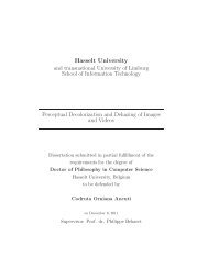
Fig. 3: Creating WBSDF from microstructure. (a) A simple sinusoidal grating<br />
is represented as a phase function. (b) Its WDF in position–spatial frequency<br />
(x, u) domain, where red defines positive values and blue negative<br />
(c) We convert the vertical slices into plots <strong>for</strong> incoming and outgoing angle,<br />
creating the WBSDF (shown at three different locations on the microstructure)<br />
(d) Rendering using this WBSDF. Top-right shows a photo <strong>for</strong> visual<br />
validation.<br />
contains only real values, positive as well as negative, since the<br />
mutual intensity is Hermitian. In this section we use a 1D function<br />
as input to explain the concept of using the WDF, but the extension<br />
to a 2D input signal is straight<strong>for</strong>ward as<br />
��<br />
Wt(x, y, u, v) = J(x, y, x ′ , y ′ )e −i2π(x′ u+y ′ v) ′ ′<br />
dx dy , (4)<br />
where<br />
J(x, y, x ′ , y ′ �<br />
) = t x + x′<br />
�<br />
y′<br />
, y + t<br />
2 2<br />
∗<br />
�<br />
x − x′<br />
�<br />
y′<br />
, y − . (5)<br />
2 2<br />
The essence of this representation is that a complex wavefront<br />
is decomposed into a series of plane waves with spatial frequency<br />
u and a real-valued amplitude. This spatial frequency corresponds<br />
to the direction of the parallel wavefront [Goodman 2005] as illustrated<br />
in Figure 2(a-b). The local spatial frequency is related to<br />
the wavelength and the direction of wave; which is normal to the<br />
wavefront, as<br />
u =<br />
sin θi<br />
. (6)<br />
λ<br />
The WDF is often used <strong>for</strong> describing the wavefront arising from<br />
surfaces like a grating. If a plane wave (i.e. light from a point light<br />
source at infinity) hits a surface, the outgoing wavefront function<br />
Rt can be described with the WDF using Eq. (2) as<br />
Rt(x, u) = Wt(x, u) (7)<br />
When a more complex wavefront hits the surface, we have to<br />
decompose the incoming wavefront Ri into plane waves and trans<strong>for</strong>m<br />
each to reconstruct the outgoing wavefront. This trans<strong>for</strong>mation<br />
is similar to the rendering equation:<br />
�<br />
Ro(x, uo) = Wt(x, uo, ui)Ri(x, ui)dui, (8)<br />
where Ro is the transmitted wavefront <strong>for</strong> an incoming wavefront<br />
Ri. Wt(x, uo, ui) is solely dependent on the microstructures of geometry<br />
t(x). Under the assumption that the structure is sufficiently<br />
thin, this trans<strong>for</strong>mation becomes angle shift–invariant; the transmitted<br />
pattern simply rotates with the incident rays. Note that this<br />
ACM Transactions on Graphics, Vol. 28, No. 4, Article 106, Publication date: August 2009.<br />
property does not necessarily imply isotropy, as the transmitted<br />
wavefront does not have to be symmetric. An angle–shift invariance<br />
assumption is valid when the lateral size of a patch is significantly<br />
larger than the thickness of the microstructure. Under this<br />
assumption the transmission function is given by<br />
�<br />
Ro(x, uo) =<br />
Wt(x, uo − ui)Ri(x, ui)dui. (9)<br />
This trans<strong>for</strong>mation is also calculated using the WDF as in Eq (2).<br />
Note that Wt(x, u) may contain positive as well as negative<br />
real–valued coefficients. However, after the integration over a<br />
finite neighborhood, the intensity value always becomes non–<br />
negative [Bastiaans 1997]. For reflections we assume that the reflected<br />
wavefront is a mirror of the transmitted wavefront, and<br />
there<strong>for</strong>e:<br />
�<br />
Ro(x, uo) = Wt(x, −uo − ui)Ri(x, ui)dui. (10)<br />
This leads to the light transport defining wave rendering equation<br />
<strong>for</strong> thin microstructures (compare with Eq. (1)),<br />
�<br />
Ro(x, uo) = Re(x, uo)+<br />
Wt(x, −uo−ui)Ri(x, ui)dui. (11)<br />
2.1 Converting Microstructures to WBSDF<br />
In order to create the WBSDF, we need to know the exact microstructure<br />
t(x) of the material. The microstructure is defined by<br />
an amplitude a(x) and phase Φ(x) with<br />
t(x) = a(x)e iΦ(x) . (12)<br />
Equation (12) allows us to calculate the WDF <strong>for</strong> the microstructure<br />
by Eq. (2). Finally, the BSDF is calculated using a basis trans<strong>for</strong>mation<br />
as<br />
�<br />
ρ(x, θi, θo, λ) ∼ W x, ± sin θo<br />
�<br />
− sin θi<br />
, (13)<br />
λ<br />
with positive sin(θo) in the case of transmission and negative <strong>for</strong><br />
reflection.<br />
The amplitude a(x) of the microstructure defines transmissivity,<br />
reflectivity and absorption. For example, an open aperture is a<br />
function that is 1 within the opening and 0 elsewhere. The component<br />
Φ(x) indicates the phase delay introduced by the refractive<br />
index or the thickness of the material at position x. Figure 3(a)<br />
illustrates the phase function <strong>for</strong> a sinusoidal grating in 2D.<br />
Figure 17 in the Appendix B shows an example in audio rendering<br />
where the reflected wall consists of two different materials with<br />
different absorption levels and different heightmaps.<br />
As an example, consider the sinusoidal grating in Figure 3. We<br />
can <strong>for</strong>mulate the microsurface as [Abramowitz and Stegun 1965]<br />
t(x) = e i m 2 sin(2π x p ) =<br />
∞�<br />
q=−∞<br />
Jq<br />
�<br />
m<br />
�<br />
e<br />
2<br />
i2πq x p (14)<br />
where m is the peak-to-peak phase excursion of the grating, p is<br />
the period and Jq is the Bessel function [Goodman 2005]. Using
Eq. (2) we can calculate its Wigner Distribution Function as<br />
W (x, u) =<br />
∞�<br />
∞�<br />
q1=−∞ q2=−∞<br />
Jq1<br />
× e i2π x p (q1−q2) δ<br />
�<br />
m<br />
� �<br />
m<br />
�<br />
Jq2<br />
2 2<br />
�<br />
u − q1<br />
�<br />
+ q2<br />
. (15)<br />
2p<br />
As a final step we convert this to the Wave BSDF using Eq. (13).<br />
2.2 Creating a Statistical WBSDF<br />
We can easily express the microstructure <strong>for</strong> a simple surface.<br />
Eq. (2) implies that the BSDF can be computed if the exact surface<br />
profile of the material is known. However, the exact microstructure<br />
may not be known <strong>for</strong> challenging objects. One way to circumvent<br />
this problem is to represent such surfaces statistically via autocorrelation<br />
and standard deviation (articulating periodicity and roughness,<br />
respectively). In this situation, we can compute the WBSDF<br />
with a statistical average as<br />
Wt(x, u) =<br />
� �<br />
t<br />
�<br />
x + x′<br />
2<br />
�<br />
t ∗<br />
�<br />
x − x′<br />
� �<br />
e<br />
2<br />
−i2πx′ u ′<br />
dx , (16)<br />
where 〈 〉 denotes average. Depending on the surface properties and<br />
rendering environments, different types of statistical averaging can<br />
be used. In general, Gaussian statistics is assumed and statistical<br />
parameters such as standard deviation σ or autocorrelation length<br />
can be tuned. Typically a standard deviation of height σh is normalized<br />
by the wavelength λ of light as<br />
σ = σh<br />
. (17)<br />
λ<br />
This statistical average approach has been used in the diffraction<br />
shader [Stam 1999] and BRDF estimators [Hoover and Gamiz<br />
2006]. According to Goodman [1984], who calculated the statistical<br />
properties of laser speckles based on the tangent–plane approximation,<br />
the surface field can be expressed as<br />
t(x) = a(x)e ik ix e 2πi<br />
λ (1+cosθ i)h(x)<br />
(18)<br />
= a(x)e ik ix e iα(x) . (19)<br />
where ki is the center wave vector incident at the elevation angle θi<br />
and h(x) is the height difference between the tangent–plane and the<br />
actual surface as illustrated in Figure 4. We assume no shadowing<br />
and no multiple interreflections. Also, the roughness should be σ ≫<br />
1.<br />
From Eq. (19) we can derive the phase variance<br />
σ 2 α = [2πσ(1 + cos θi)] 2<br />
(20)<br />
and the phase autocorrelation<br />
Rα(x ′ � �2 2π<br />
) = (1 + cos θi) Rh(x<br />
λ ′ ), (21)<br />
where Rh(x ′ ) is the autocorrelation of the surface height (Figure<br />
11(a)). If we assume a Gaussian distribution of surface<br />
height we can now <strong>for</strong>mulate the correlation function. Note that<br />
〈t (x + x ′ /2) t ∗ (x − x ′ /2)〉 is mutual intensity J(x, x ′ ).<br />
J(x ′ ) = e ik ix ′<br />
〈e iα(x)−α(x−x′ ) 〉 (22)<br />
= e ik ix ′<br />
e −σ2 α[1−ρ h(x ′ )] , (23)<br />
<strong>Reflectance</strong> <strong>Model</strong> <strong>for</strong> <strong>Diffraction</strong> • 5<br />
N<br />
θ i<br />
h(x)<br />
k i<br />
incident<br />
wave<br />
tangent<br />
plane<br />
microstructure<br />
Fig. 4: A schematic overview of the approximated surface field, where ki<br />
is the center wave vector incident at the elevation angle θi. h(x) represents<br />
the height difference from the target plane to the actual surface.<br />
where<br />
ρh(x ′ ) = Rh(x ′ )<br />
σ2 . (24)<br />
h<br />
Since the WDF is defined with respect to the correlation function<br />
as in Eq. (2), we can derive the WBSDF from the WDF of the<br />
correlation function as<br />
�<br />
Wγ(u) = J(x ′ )e −i2πu·x′<br />
dx ′<br />
= e −σ2 � � 2<br />
αF<br />
σα exp<br />
σ2 Rh(x<br />
h<br />
′ )<br />
�� � � ���x ′ →u− sin θ i<br />
λ<br />
. (25)<br />
An overview to calculate the Wave BSDF based on the microstructure<br />
geometry is illustrated in Figure 5.<br />
2.3 Benefits<br />
Near and far field: The WDF as well as the WBSDF are<br />
conserved along rays in the paraxial region [Bastiaans 2009],<br />
hence they are valid in both the near-field and far-field. In the<br />
far-field, the observed wave at a single point is only dependent<br />
on angle, and is essentially independent of the distance from<br />
diffracting surface. Near-field corresponds to the Fresnel region<br />
in optics (not to be confused with the near-zone in optics where<br />
the evanescent field is still strong). The near-field is the region<br />
close to the diffracting surface, where the wave’s distance to the<br />
grating also influences the observed pattern. In contrast to previous<br />
diffractive BRDFs [Stam 1999], the WBSDF does not require an<br />
assumption that the object and receiver are at infinity. Near field<br />
effects, such as the PSF of lenses, require more computation than<br />
far field effects. Hence, importance sampling is highly desired. As<br />
Exact geometry<br />
known<br />
Yes<br />
No h<br />
Calculate t(x) from<br />
geometry using eq 12<br />
Define geometry<br />
statistically:<br />
* R : autocorrelation<br />
surface height<br />
* σ : standard deviation<br />
α<br />
Calculate W(x,u)<br />
using eq 2<br />
Calculate W(u)<br />
using eq 25<br />
Calculate BSDF<br />
Using eq 13<br />
Fig. 5: A schematic overview to calculate the WBSDF based on the exact<br />
or statistically estimated microsurface geometry.<br />
ACM Transactions on Graphics, Vol. 28, No. 4, Article 106, Publication date: August 2009.
6 • T. Cuypers et al.<br />
Single beam Single beam<br />
(a)<br />
(b)<br />
Single beam<br />
Bundle<br />
(c)<br />
(d)<br />
R i1<br />
R i2<br />
R i2 R i3<br />
Interference<br />
R o1 Ro2 Ro3<br />
Fig. 6: <strong>Diffraction</strong> shaders is a special case of the WBSDF. (a–b) It preencodes<br />
the result of far-field interference into energy of the outgoing ray.<br />
These rays cannot destructively interfere anymore in a later stage. (c–d)<br />
WBSDF indirectly encodes phase in<strong>for</strong>mation into the outgoing ray by introducing<br />
potentially negative radiance, allowing the rays to interfere later<br />
<strong>for</strong> global illumination.<br />
a result, our technique is also applicable <strong>for</strong> simulating acoustics,<br />
as its derivation is similar to ray–based audio rendering.<br />
Importance sampling and global illumination: The WBSDF<br />
uses instantaneous diffraction; i.e., the magnitude of energy<br />
scattered in all directions is known at the surface. This allows<br />
importance sampling <strong>for</strong> an efficient light or audio simulation and<br />
is also suitable <strong>for</strong> rendering global illumination.<br />
Light coherence: Natural scenes are composed of incoherent<br />
sources. This means that each single point source is mutually incoherent<br />
with other point sources. Simulating interference effects<br />
normally requires rendering the scene <strong>for</strong> each light source independently,<br />
and then summing up images to create the final result.<br />
Because creating diffractive effects <strong>for</strong> a single light source only<br />
consists of summing up photons (positive or negative), our technique<br />
can simultaneously render coherent light as well as multiple<br />
incoherent light sources, such as area lights. In rare scenarios, multiple<br />
sources are mutually coherent. Here, we treat all the sources<br />
jointly to compute a single emissive WBSDF (see Appendix B).<br />
2.4 Limitations<br />
We use the paraxial approximation, where incoming and scattered<br />
(diffracted) light propagate not far from the optical axis. To improve<br />
the accuracy in the non–paraxial zone, one can use the angle–<br />
impact WDF [Alonso 2004]. Regarding polarization, we only consider<br />
linearly polarized light. Adopting the coherency matrix [Tannenbaum<br />
et al. 1994], we can extend our method beyond linearly<br />
polarized light. The current model of the WDF only encodes spatially<br />
varying phase and does not take temporal phase into account.<br />
Using the WBSDF, a single reflected ray off a surface may contain<br />
negative radiance, which is physically impossible. However,<br />
by integrating over a finite neighbourhood, <strong>for</strong> example in a camera<br />
aperture, the total amount of received light always becomes non–<br />
negative due to the properties of the WDF [Bastiaans 2009]. There<strong>for</strong>e,<br />
our model does not support pinhole camera models <strong>for</strong> direct<br />
lighting. More details on this topic are presented in the supplemental<br />
material.<br />
2.5 Relationship with <strong>Diffraction</strong> Shaders<br />
<strong>Diffraction</strong> shaders (DS) pioneered the idea of fast and practical<br />
rendering of the far field diffraction of a single bounce [Stam 1999].<br />
ACM Transactions on Graphics, Vol. 28, No. 4, Article 106, Publication date: August 2009.<br />
It turns out that the DS approach is a special case of our method<br />
where the light source and the observer are at infinity. DS converts<br />
parallel ray bundles predicted by the WBSDF and treats them as a<br />
single ray beam (Figure 6). The WBSDF maintains a higher resolution<br />
representation and hence we can apply different integration<br />
kernels, trans<strong>for</strong>ms <strong>for</strong> propagation, and scattering models. The<br />
WBSDF also provides flexibility depending on incident/outgoing<br />
rays, camera geometry, computational speed and tolerance of error.<br />
The WBSDF supports a statistical model similar to the one used<br />
in DS <strong>for</strong> phase variations. Based on the assumption that the light<br />
source and the observer are at infinity, we use the same notation as<br />
in Ref. [Stam 1999] and present the relationship with the WBSDF<br />
as follows:<br />
I (ku ′ ) = ψ (ku ′ ) ψ ∗ (ku ′ )<br />
�<br />
= e ikwh(x) e iku′ �<br />
x<br />
dx e −ikwh(x′ ) −iku<br />
e ′ x ′<br />
dx ′<br />
��<br />
=<br />
q<br />
ikwh(p+<br />
e 2 ) q<br />
−ikwh(p−<br />
e 2 ) e iku′ q<br />
dpdq<br />
�<br />
= Wd(x, u ′ )dx, (26)<br />
where I is intensity, ψ is field, k = 2π/λ, u ′ = sin θ1−sin θ2, w =<br />
− cos θ1 −cos θ2, p = (x+x ′ )/2, q = x−x ′ , and Wd(x, u ′ ) is the<br />
WDF of eikwh(x) with respect to sin θ1 − sin θ2, which represents<br />
the reflectance of the surface. In our <strong>for</strong>mulation, as mentioned in<br />
Sec. 2, the outgoing WDF is written as<br />
�<br />
Ro (x, uo) = Wt (x, uo; ui) R (x, ui) dui. (27)<br />
Assuming that a plane wave is incident on a surface (Ri(x, ui) =<br />
δ(ui − sin θi/λ)) and the observer is at infinity as in the diffraction<br />
shader equations (uo = sin θo/λ), we obtain the reflected light as<br />
�<br />
�<br />
I(uo) = Ro(x, uo)dx =<br />
3. IMPLEMENTATION<br />
Wt<br />
�<br />
x,<br />
sin θo sin θi<br />
;<br />
λ λ<br />
�<br />
dx. (28)<br />
We achieve global illumination effects using an unmodified PBRT<br />
framework [Pharr and Humphreys 2004]. The only minor change<br />
is that we comment out the check <strong>for</strong> non-negative radiance. To<br />
generate specific diffractive material, we simply created a new material<br />
plugin <strong>for</strong> PBRT.<br />
We used photon mapping <strong>for</strong> Monte Carlo simulation of global<br />
illumination. Due to the nature of this technique, photon mapping<br />
per<strong>for</strong>ms well with our BSDF. Photons can convey negative energy<br />
to achieve destructive interference. WDF <strong>for</strong>mulation ensures that<br />
non–negative final energy is gathered at a single point. This non–<br />
negativeness also applies to the gathering of photons in the photon<br />
map.<br />
Sinusoidal grating<br />
Figure 3(d)<br />
Single CD<br />
Figure 4(a)<br />
CDs<br />
Figure 4(b)<br />
Teaser<br />
Figure 1<br />
CD on GPU<br />
Figure 11<br />
# photons 10M 5M 50M 1M Not applicable<br />
Rendering time 5100 s 1500 s 4400 s 1700 s 35 fps<br />
Table II. : Rendering time and number of photons used <strong>for</strong> each scene.<br />
Implementation is done using PBRT. All these scenes are rendered single<br />
threaded on a 3GHz core. The GPU example was done on a NVidia 8400M<br />
with 640×480 resolution.
For materials with a separable WBSDF <strong>for</strong> x and y coordinates,<br />
we precomputed the WBSDF and saved it as a 2D look–up table,<br />
which allows fast calculation, importance sampling (Figure 7), and<br />
real-time rendering of single bounce diffraction on the GPU (Figure<br />
8). As diffration has to be calculated on arrival, we need to<br />
sample over different locations <strong>for</strong> each pixel and integrate the values.<br />
Mipmapping calculates these interference effects efficiently.<br />
Similar to the diffraction shader implementation [Stam 1999], the<br />
colorfull 0th order highlight is added with a simple anisotropic<br />
shader [Ward 1992]. Table II gives an overview of rendertime used<br />
<strong>for</strong> generating the images and audio examples. The pdf is calculated<br />
using the absolute values of the intensity in the BRDF lookup<br />
table.<br />
(a) Without importance sampling (b) With importance sampling<br />
Fig. 7: Benefits of importance sampling (a) Without importance sampling,<br />
even after 14,000 s result does not converge (b) With, 1,300 s.<br />
Eq. (13) provides a function in position, angle, and wavelength.<br />
For structured surfaces, like sinusoidal gratings, we have a closed<br />
<strong>for</strong>m solution to find which wavelengths have non–zero intensities.<br />
For computational efficiency, we tabulated the WBSDFs in terms<br />
of position and angle, and reduced the wavelengths to RGB values<br />
according to the camera response curves. The lookup tables, used<br />
<strong>for</strong> creating the examples in this paper, have a sampling rate of<br />
0.02 ◦ in angular domain and 48 nm in the spatial domain. For<br />
non–structured surfaces such as rainbow holograms, we computed<br />
Eq. (13) over 30 wavelengths and stored only RGB values using<br />
the appropriate weights.<br />
Validation We compared two representative diffraction examples<br />
with the one computed by Fourier optics and verified the accuracy<br />
of our technique. We used photon mapping to simulate Young’s<br />
double slit experiment and light diffraction from a rectangular aperture<br />
(Fraunhofer diffraction). The absolute intensity error, mainly<br />
due to limited numerical precision, between the Fraunhofer diffrac-<br />
Fig. 8: CD rendered using the WBSDF in real-time on a GPU using look-up<br />
tables and mipmapping.<br />
<strong>Reflectance</strong> <strong>Model</strong> <strong>for</strong> <strong>Diffraction</strong> • 7<br />
tion pattern and the rendering with the WBSDF is less than 1%.<br />
These results are presented in Figure 9.<br />
a<br />
Real Image Rendering<br />
Fig. 9: Validation of the WBSDF (a) Visual comparison of photo and rendering<br />
of diffraction due to a laser through a rectangular aperture. (b) Rendering<br />
of (a) and its 1D plot. (c) Two slit experiment and 1D plot. The 1D<br />
plots are compared with the Fraunhofer diffraction and have an absolute<br />
intensity error of less than 1%.<br />
4. RESULTS<br />
We show representative ray–based wave effect rendering as examples<br />
<strong>for</strong> global illumination.<br />
4.1 Light Rendering<br />
<strong>Diffraction</strong> and interference: The WBSDF indirectly retains<br />
the phase in<strong>for</strong>mation after diffraction, and defers the interference<br />
computation. This strategy supports interference after global illumination<br />
naturally. Figure 1 shows the diffracted wavefront from<br />
a CD undergoing refraction. As we describe later, instantaneous<br />
diffraction enables importance sampling.<br />
Figure 10 shows 2 CDs interacting with each other and illuminating<br />
a wall. We model the CD as a phase grating with a pitch of<br />
2 µm. We believe this is the first practical demonstration of global<br />
illumination of wave phenomenon, which is achieved using an unmodified<br />
PBRT.<br />
Figure 11 demostrates the statistical approach of the BSDF. In<br />
the autocorrelation of the surface we used the function<br />
b<br />
c<br />
Rh = −(x/a) 4 , (29)<br />
as shown in Figure 11(a). The BSDF is calculated <strong>for</strong> θin and θout<br />
(Figure 11(b)) and mapped onto spheres, each with a different<br />
Fig. 10: Renderings using the WBSDF under global illumination. (Left)<br />
Light reflected off a CD on a diffuse wall, (Right) light emitted from an<br />
area light (top) is reflected off the left CD onto the right CD and then to the<br />
floor.<br />
ACM Transactions on Graphics, Vol. 28, No. 4, Article 106, Publication date: August 2009.
8 • T. Cuypers et al.<br />
a)<br />
0 100 200<br />
θ o<br />
in um<br />
θ i<br />
b) c)<br />
2<br />
3<br />
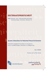
Fig. 11: Rendered results using the statistical approach of the WBSDF. (a)<br />
Example Rh function describing the basic surface height of elements to<br />
reconstruct the microstructure. (b) The statistical WBSDF of element (a)<br />
plotted in θi and θo <strong>for</strong> a specific standard deviation. (c) Rendered result of<br />
spheres on which this BRDF is mapped. Spheres 1 to 4 have respectively a<br />
standard deviation of 10, 8, 6 and 4.<br />
standard deviation.<br />
Rainbow holograms: As we can create the WBSDF of any<br />
diffractive optical element based on its microstructure, we can derive<br />
a WBSDF <strong>for</strong> a holographic surface as well. As diffraction is<br />
computed instantaneously <strong>for</strong> the entire surface, we do not keep<br />
track of travel distance from a given point to the hologram surface,<br />
as OPD does. The hologram can be rendered directly from the WB-<br />
SDF and creates interference inside the aperture of the camera lens.<br />
Note that there are many different ways of computing the WDF of<br />
the object [Plesniak and Halle 2005]. For simplicity, here we encoded<br />
incoherent objects in the hologram; however any arbitrary<br />
wavefront in<strong>for</strong>mation can be stored in the WBSDF. The rainbow<br />
hologram, invented by Benton [1969], is reconstructed by white<br />
light and exhibits only the horizontal parallax. Considering the desired<br />
hologram signal, we obtain the WDF of the hologram as<br />
Wh(x, y, u, v) = Wobj(x + λrz0u, y + λz0(v + v0), uv + v0)<br />
� �<br />
v + v0<br />
rect<br />
(30)<br />
A/(zAλr)<br />
where Wobj is the WDF of the object being recorded. We can derive<br />
this function from the constructed lightfield using eq. ( 6). The<br />
parameter z0 is the distance between the reconstructed object and<br />
Fig. 12: Rainbow hologram renderings from different viewpoints. Instantaneous<br />
diffraction using the WBSDF pre-computes the view–dependent<br />
appearance.<br />
ACM Transactions on Graphics, Vol. 28, No. 4, Article 106, Publication date: August 2009.<br />
1<br />
4<br />
Fig. 13: An overview of the creation of a rainbow hologram. (a) The first<br />
hologram is recorded containing the object in<strong>for</strong>mation. (b) The second<br />
hologram is constructed via a horizontal slit. (c) The reconstruction hologram<br />
looks as if we are looking through a slit at the object, allowing the<br />
reflection only in a narrow viewing angle.<br />
the second hologram, zA is the distance between the second hologram<br />
and the slit, λr is the recording wavelength, and v0 is the<br />
spatial frequency along the vertical direction of the second reference<br />
wave. The rectangular function in eq. (30) is derived from the<br />
recorded slit with an aperture size of A. These are shown in Figure<br />
13.<br />
4.2 Simulating Camera Optics<br />
In camera optics, aberrations as well as diffraction affect the Point<br />
Spread Function (PSF) of the system. Hence, conventional optics<br />
design software provides analytical tools <strong>for</strong> aberrations and<br />
diffraction. However, they treat the two separately; i.e., ray tracing<br />
uses spot diagrams as an estimate of the PSF, whereas diffraction<br />
models produce PSFs directly from Fourier optics analysis. Note<br />
that a Fourier optics analysis typically assumes a shift invariant<br />
PSF, hence the diffraction <strong>for</strong> an off–axis PSF is assumed to be<br />
identical to the on–axis PSF, which is not true in practice.<br />
In addition to Oh et. al. [2010], our approach can simulate both<br />
aberrations and diffraction simultaneously <strong>for</strong> any location of the<br />
image plane, since it is based on ray–representation and able to<br />
include diffraction. We derived the WBSDF from the geometric<br />
structure of a camera lens with a circular aperture and calculated<br />
the PSF. The Wigner Distribution Function of a 2D circular aperture<br />
was described by Bastiaans and Mortel [Bastiaans and van de<br />
Mortel 1996]. Figure 14 shows spatially varying PSFs <strong>for</strong> different<br />
lenses and point light positions. We then applied the PSFs to a<br />
computer generated image by convolution, simulating the appearance<br />
of the scene when viewed with this lens. Note that in this<br />
example, no chromatic aberration was assumed. Hence, the color<br />
dispersion results solely from diffraction. Although, we only consider<br />
thin lenses in this particular example, we can easily simulate<br />
a series of thick lenses as well. The global illumination ray–tracing<br />
takes care of refraction at air–glass interfaces and diffraction by an<br />
aperture is included by the WBSDF.<br />
5. COMPARISON<br />
5.1 Comparison with OPD<br />
Even though optical path difference (OPD) provides accurate results<br />
of interference, it requires significant modifications to traditional<br />
rendering systems and is not able to per<strong>for</strong>m importance<br />
sampling. Traditional raytracers commonly do not take distance or<br />
phase into account, and in order to implement OPD we need to<br />
make changes to the framework. The precision required <strong>for</strong> path<br />
length (<strong>for</strong> each wavelength) becomes challenging. In addition,<br />
OPD cannot exploit importance sampling. Determining the propagation<br />
direction of rays with dominant intensity in the presence of<br />
diffraction is challenging. OPD-based techniques must uni<strong>for</strong>mly
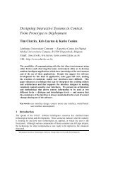
f / 5.6<br />
f / 11<br />
on axis o� axis on axis o� axis<br />
Fig. 14: Near field effects in camera lenses show the effect of an aperture<br />
creating diffraction and chromatic dispersion. (Left) PSFs of F/5.6 lens <strong>for</strong><br />
lights at two different depths. (Right) PSFs of F/11 lens <strong>for</strong> two different<br />
depths.<br />
sample all the outgoing directions. Consider the example of the sinusoidal<br />
gratings of Figure 3. The WBSDF reveals the few important<br />
directions using our instantaneous diffraction theory. In more<br />
complex, global illumination settings, WBSDF-based approach is<br />
faster compared to OPD by the same factor as shown in Figure 7.<br />
5.2 Comparison with <strong>Diffraction</strong> Shaders<br />
As shown in section 2.5, <strong>Diffraction</strong> shaders [Stam 1999] is a special<br />
case of the Wave BSDF. In the implementation of diffraction<br />
from CDs, we assumed angle–shift invariance, where the phase<br />
function ψ(x) does not depend on the incident angle. If we use<br />
the same setup assumptions as DS (i.e., a plane wave incident on a<br />
camera at sufficiently far distance), then our result is comparable to<br />
the one generated by DS, especially in the paraxial region.<br />
The WBSDF analysis also points to new ways to improve the<br />
DS approach. DS can now be used <strong>for</strong> transmission using Eqs. (9)<br />
and (10). In the examples generated by DS, height–maps were used<br />
to model phase delays <strong>for</strong> pre–computing interference from parallel<br />
light rays, ignoring the amplitude component of the microstructure.<br />
The amplitude controls the amount of light that is absorbed or scattered.<br />
To account <strong>for</strong> the amplitude variation, we can add an a(x)<br />
term in Eq. (12). Despite these extensions, DS remains applicable<br />
only in the far field, since the integration is already per<strong>for</strong>med. DS<br />
is also less suitable <strong>for</strong> simulating audio diffraction (large wavelength)<br />
or simulating a PSF of a camera’s optics (larger integrating<br />
cone <strong>for</strong> receiving patch).<br />
5.3 Comparison with Augmented Light Fields<br />
Augmented light fields [Oh et al. 2010] (ALF) is the first model<br />
to use the WDF <strong>for</strong> rendering. It uses a simplistic two plane light<br />
field parametrization: one <strong>for</strong> diffraction grating plane and one <strong>for</strong><br />
receiver plane. Hence, it is limited to demonstrations of a planar<br />
wavefront transmitted via the first plane of a diffractive occluder.<br />
They use a ’destination based’ approach (i.e. differed diffraction)<br />
using an OpenGL fragment shader. The ALF is computed in a backward<br />
manner: at each point on the receiver, the shader computes<br />
the incident ray-bundle (slice of the lightfield) using an analytical<br />
<strong>for</strong>mula <strong>for</strong> the diffraction pattern from the source towards the<br />
receiver. This differed diffraction is very similar to OPD, so it provides<br />
no importance sampling and the paths to trace grow exponen-<br />
<strong>Reflectance</strong> <strong>Model</strong> <strong>for</strong> <strong>Diffraction</strong> • 9<br />
tially with each bounce. The ALF work suggests photon mapping<br />
as a possible extension, but it is treated as a procedure that would<br />
modify the scatter stage of a renderer. By encoding a new BSDF, we<br />
make no change to the renderer. Instead of a new rendering strategy,<br />
WBSDF encodes the microstructure into a new reflectance function<br />
independent of other elements or illumination in the scene. This allows<br />
a wide range of effects not shown with ALF such as reflection,<br />
emission, multi-bounce, importance sampling, sound rendering and<br />
a natural fit with the rendering equation. Refer to Table I <strong>for</strong> more<br />
details.<br />
5.4 Comparison with Edge–diffraction<br />
Edge diffraction is a rudimentary <strong>for</strong>m of importance sampling<br />
used in audio rendering. It can be improved by using the WB-<br />
SDF as shown in Figure 15. This becomes even more significant<br />
when phase is involved, such as the example of the array of speakers<br />
in Figure 18. Edge diffraction techniques underestimate mid–air<br />
diffraction and allow strong ray bending at edges, whereas our technique<br />
creates diffraction through entire features, ensuring accurate<br />
diffraction results. Edge diffraction cannot achieve the unusual effect<br />
of the sound of a door closing. Our current method does not<br />
take traveling distance into account and as a result does not exhibit<br />
damping.<br />
Θ<br />
(a) (b) (c) (d)<br />
x<br />
Fig. 15: WBSDF is more accurate than edge diffraction. (a) Edge diffraction<br />
only diffracts rays at corners and (b) ignores mid–air diffraction. (c–d)<br />
WBSDF creates midair diffraction.<br />
6. CONCLUSION<br />
We describe a new representation of BSDF that greatly simplifies<br />
simulations of wave-phenomena in ray-based renderers. We<br />
bring the wave phenomena into the realm of the rendering-equation<br />
which supports global illumination, including benefits such as importance<br />
sampling. Additionally, we provide a detailed comparison<br />
of many wave phenomena renderers. We feel that we have methodically<br />
investigated the rendering of wave phenomena by proposing<br />
an easy and efficient solution, demonstrated examples in multiple<br />
domains (light/sound), investigated and solved implementation issues,<br />
and mathematically expressed out work’s relationship with<br />
diffraction shaders.<br />
We see many promising directions <strong>for</strong> future exploration. The<br />
WBSDF can be used <strong>for</strong> other areas of spectrum such as microwaves<br />
and x–rays or other wave–related disciplines, including<br />
the transient response <strong>for</strong> fluid wave diffraction. The simulation of<br />
camera optics can be extended to support a full camera model in existing<br />
rendering frameworks. Sound rendering extensions include<br />
attenuation, reverberation, non-planar area sources, Doppler effect<br />
and modeling of head-related transfer function (HRTF) using our<br />
<strong>for</strong>mulation <strong>for</strong> easy ray-based analysis. Advanced surface scattering<br />
models, will potentially extend the applications of the WBSDF<br />
and improve the accuracy to the physical models. Although current<br />
reflectance field scanning methods use a ray-based understanding,<br />
we hope WBSDF methods will inspire novel capture and inverse<br />
ACM Transactions on Graphics, Vol. 28, No. 4, Article 106, Publication date: August 2009.<br />
Θ<br />
x
10 • T. Cuypers et al.<br />
problems in analysis of real world objects exhibiting wave phenomena.<br />
ACKNOWLEDGMENTS<br />
Tom Cuypers, Tom Haber and Philippe Bekaert acknowledge financial<br />
support by the European Commision (FP7 IP 2020 3D Media),<br />
the Flemish Interdisciplinary Institute <strong>for</strong> Broadband Technology<br />
(IBBT) and the Flemish Government. Ramesh Raskar is supported<br />
by an Alfred P. Sloan Research Fellowship and by DARPA Young<br />
Faculty Award . Se Baek Oh’s current affiliation is KLA-Tencor<br />
corporation, Milpitas, CA.<br />
REFERENCES<br />
ABRAMOWITZ, M. AND STEGUN, I. A. 1965. Handbook of Mathematical<br />
Functions with Formulas, Graphs, and Mathematical Tables. New York.<br />
ALONSO, M. A. 2004. Wigner functions <strong>for</strong> nonparaxial, arbitrarily polarized<br />
electromagnetic wave fields in free space. Journal of Optical Society<br />
of America A 21, 11, 2233–2243.<br />
BASTIAANS, M. 1997. Application of the wigner distribution function in<br />
optics. In The Wigner Distribution - Theory and Applications in Signal<br />
Processing. Elsevier Science.<br />
BASTIAANS, M. J. 1977. Frequency-Domain Treatment of Partial Coherence.<br />
Optica Acta 24, 3, 261–274.<br />
BASTIAANS, M. J. 2009. Wigner distribution in optics. In Phase-Space<br />
Optics: Fundamenals and Applications, M. Testorf, B. Hennelly, and<br />
J. Ojeda-Castañeda, Eds. McGraw-Hill, New York, 1–44.<br />
BASTIAANS, M. J. AND VAN DE MORTEL, P. G. J. 1996. Wigner distribution<br />
function of a circular aperture. J. Opt. Soc. Am. A 13, 8, 1698–1703.<br />
BENTON, S. A. 1969. Hologram reconstruction with extended incoherent<br />
sources. Journal of Optical Society of America 59, 1545–1546.<br />
CHANDAK, A., LAUTERBACH, C., TAYLOR, M., REN, Z., AND<br />
MANOCHA, D. 2008. Ad-frustum: Adaptive frustum tracing <strong>for</strong> interactive<br />
sound propagation. IEEE Transactions on Visualization and Computer<br />
Graphics 14, 6, 1707–1722.<br />
DACHSBACHER, C., STAMMINGER, M., DRETTAKIS, G., AND DURAND,<br />
F. 2007. Implicit visibility and antiradiance <strong>for</strong> interactive global illumination.<br />
ACM SIGGRAPH 26, 3 (August).<br />
FRENIERE, E. R., GREGORY, G. G., AND HASSLER, R. A. 1999. Edge<br />
diffraction in monte carlo ray tracing. Proc. SPIE Vol. 3780, Optical<br />
Design and Analysis Software, 151–157.<br />
GOODMAN, J. W. 1984. Statistical properties of laser speckle patterns.<br />
In Laser Spekcle and Related Phenomena, 2nd ed., J. C. Dainty, Ed.<br />
Springer Verlag, Chapter 2.<br />
GOODMAN, J. W. 2005. Introduction to Fourier optics, 3rd ed. Roberts &<br />
Co., Englewood, Colo.<br />
HOOVER, B. G. AND GAMIZ, V. L. 2006. Coherence solution <strong>for</strong> bidirectional<br />
reflectance distribution of surfaces with wavelength–scale statistics.<br />
Journal of Optical Society of America A 23, 314–328.<br />
HOTHERSALL, D., CHANDLER-WILDE, S., AND HAJMIRZAE, M. 1991.<br />
Efficiency of single noise barriers. In Journal of Sound and Vibration.<br />
JENSEN, H. W. 1996. Global illumination using photon maps. In Eurographics<br />
workshop on Rendering techniques. Springer-Verlag, London,<br />
UK, 21–30.<br />
JENSEN, H. W. AND CHRISTENSEN, P. H. 1998. Efficient simulation of<br />
light transport in scences with participating media using photon maps. In<br />
Proceedings of SIGGRAPH 1998. ACM, 311–320.<br />
KAJIYA, J. T. 1986. The rendering equations. In Computer Graphics (Proceedings<br />
of SIGGRAPH 86). Computer Graphics (Proceedings of SIG-<br />
GRAPH 86) 20, 143–150.<br />
ACM Transactions on Graphics, Vol. 28, No. 4, Article 106, Publication date: August 2009.<br />
KOUYOUMJIAN, R. AND PATHAK, P. 1974. A uni<strong>for</strong>m geometrical theory<br />
of diffraction <strong>for</strong> an edge in a perfectly conducting surface. Proceedings<br />
of the IEEE 11.<br />
LINDSAY, C. AND AGU, E. 2006. Physically-based real-time diffraction<br />
using spherical harmonics. In Advances in Visual Computing. Springer,<br />
505–517.<br />
MORAVEC, H. P. 1981. 3d graphics and the wave theory. In Computer<br />
Grqphics (Proceedings of SIGGRAPH 81). Vol. 15. ACM, 289–296.<br />
OH, S. B., KASHYAP, S., GARG, R., CHANDRAN, S., AND RASKAR, R.<br />
2010. Rendering wave effects with augmented light fields. EuroGraphics.<br />
PHARR, M. AND HUMPHREYS, G. 2004. Physically Based Rendering:<br />
From Theory to Implementation. Morgan Kaufmann Publishers Inc., San<br />
Francisco, CA, USA.<br />
PLESNIAK, W. AND HALLE, M. 2005. Computed holograms and holographic<br />
video display of 3d data. In ACM SIGGRAPH 2005 Course.<br />
ACM, 69.<br />
RICK, T. AND MATHAR, R. 2007. Fast edge-diffraction-based radio<br />
wave propagation model <strong>for</strong> graphics hardware. In International ITG–<br />
Conference on Antennas. 15–19.<br />
SILTANEN, S., LOKKI, T., KIMINKI, S., AND SAVIOJA, L. 2007. The<br />
room acoustic rendering equation. The Journal of the Acoustical Society<br />
of America 122, 3, 1624–1635.<br />
STAM, J. 1999. <strong>Diffraction</strong> shaders. In Proceedings of SIGGRAPH 1999.<br />
Proceedings of SIGGRAPH 2001.<br />
SUN, Y. 2006. Rendering biological iridescences with RGB–based renderers.<br />
ACM Transactions on Graphics 25, 1, 100–129.<br />
SUN, Y., FRACCHIA, F. D., DREW, M. S., AND CALVERT, T. W. 2000.<br />
Rendering iridescent colors of optical disks. In EGWR. 341–352.<br />
TANNENBAUM, D. C., TANNENBAUM, P., AND WOZNY, M. J. 1994. Polarization<br />
and birefringency considerations in rendering. In ACM SIG-<br />
GRAPH 1994. 221–222.<br />
TORRES, R. R., SVENSSON, U. P., AND KLEINER, M. 2001. Computation<br />
of edge diffraction <strong>for</strong> more accurate room acoustics auralization.<br />
Acoustical Society of America Journal.<br />
TSINGOS, N. March 2000. A geometrical approach to modeling reflectance<br />
functions of diffracting surfaces. Tech. rep.<br />
TSINGOS, N., DACHSBACHER, C., LEFEBVRE, S., AND DELLEPIANE,<br />
M. 2007. Instant sound scattering. In EGSR.<br />
TSINGOS, N., FUNKHOUSER, T., NGAN, A., AND CARLBOM, I. 2001.<br />
<strong>Model</strong>ing acoustics in virtual environments using the uni<strong>for</strong>m theory of<br />
diffraction. In ACM SIGGRAPH 2001. ACM.<br />
WALTHER, A. 1973. Radiometry and Coherence. Journal of Optical Society<br />
of America 63, 12, 1622–1623.<br />
WARD, G. J. 1992. Measuring and modeling anisotropic reflection. Proceedings<br />
of SIGGRAPH 1992 26, 2, 265–272.<br />
WHITTED, T. 1980. An improved illumination model <strong>for</strong> shaded display.<br />
Commun. ACM 23, 6, 343–349.<br />
WOLF, E. 1978. Coherence and Radiometry. Journal of Optical Society of<br />
America 68, 1, 6–17.<br />
ZHANG, Z. AND LEVOY, M. 2009. Wigner distributions and how they<br />
relate to the light field. In IEEE Internatinoal Conference on Computational<br />
Photography.<br />
ZIEGLER, R., BUCHELI, S., AHRENBERG, L., MAGNOR, M., AND<br />
GROSS, M. 2007. A bidirectional light field - hologram trans<strong>for</strong>m. Computer<br />
Graphics Forum 26, 3, 435–446.<br />
ZIEGLER, R., CROCI, S., AND GROSS, M. H. 2008. Lighting and occlusion<br />
in a wave-based framework. Computer Graphics Forum 27, 2,<br />
211–220.
Appendix A<br />
Wigner distribution function <strong>for</strong> 1D element t(x), in Matlab.<br />
function W = WDF(g)<br />
N = length(t);<br />
x = (((0:N-1)-N/2)*2*pi/(N-1)); % Generate linear vector <strong>for</strong> shift<br />
X = (0:N-1)'-N/2;<br />
G1 = ifft( (fft(g)*ones(N,1)).*exp( i*x*X/2 )); % create g( x + x/2' )<br />
G2 = ifft( (fft(g)*ones(N,1)).*exp( -i*x*X/2 )); % create g( x - x/2' )<br />
W = fft(G1.*conj(G2), [], 1); % calculate WDF<br />
Appendix B: Towards Audio Rendering<br />
The same <strong>for</strong>mulation as the rendering equation exists <strong>for</strong> sound<br />
rendering and is called the room acoustic rendering equation [Siltanen<br />
et al. 2007]. The derivation <strong>for</strong> this room acoustic rendering<br />
equation is similar to section 2. We there<strong>for</strong>e show that this BSDF<br />
is applicable <strong>for</strong> audio as well under an infinite speed assumption.<br />
Transmission <strong>Diffraction</strong> becomes more significant with longer<br />
wavelengths. A common technique <strong>for</strong> rendering diffraction in audio<br />
is to per<strong>for</strong>m diffraction at only edges in the scene, thereafter<br />
keeping track of the distance traveled by the sound wave. The WB-<br />
SDF can be used <strong>for</strong> rendering transmissive and reflective audio<br />
diffraction without keeping track of the sound wave phase. Importance<br />
sampling simplifies the propagation by weighting the computational<br />
power to regions which matters most. We simulate an<br />
interesting effect where a closing sliding door modulates the sound<br />
intensity as shown in Figure 18.<br />
a) b)<br />
Intensity<br />
Door closing<br />
1m 10 cm<br />
Fig. 16: The WBSDF can also simulate transmissive effects of audio. (a) A<br />
scene where the listeren and speaker are occluded by a wall with an open<br />
door. The received audio intensity is calculated using the WBSDF (b) The<br />
observed intensity of the speaker with respect to the openingsize of the door.<br />
Reflection In Figure 17, the wall is a composition of 2 materials<br />
at 2 different depths. Figure 17(a) and (b) represents the absorption<br />
and heightmap of the wall. The result is shown on figure 1(c) and<br />
figure 17(c). Tsingos et. al. [Tsingos et al. 2007] have also shown a<br />
useful method <strong>for</strong> diffraction from high frequency structures based<br />
on Kirchhoff approximation [Tsingos et al. 2007] and their method<br />
is similar to diffraction shaders, i.e. limited to a single bounce precomputed<br />
interferrence. For simplicity, we only show diffraction<br />
effects without considering reflections.<br />
Emission We use the principle of light trans<strong>for</strong>mation to calculate<br />
the emission function Le of Eq. (1) to account <strong>for</strong> the phase delay.<br />
Amplitude Grating (absorption level)<br />
a<br />
Phase Grating (height map)<br />
b c<br />
<strong>Reflectance</strong> <strong>Model</strong> <strong>for</strong> <strong>Diffraction</strong> • 11<br />
Wall<br />
Sound<br />
Source<br />
d<br />
Intensity<br />
10 kHz<br />
0 m 3 m<br />
Fig. 17: Audio reflection from high frequency structure on a wall. (a) absorption<br />
level (b) heightmap as input textures. Total width is 60 cm. (c)<br />
Rendered scenario using heightmap and absorption level to model the wall<br />
(d) Recorded intensity at a depth of 2.8m, (red) is calculated using the WB-<br />
SDF, while (blue) is constructed using phase tracking.<br />
The relative phase delay between emitters creates a non–planar<br />
wave. This effect is highly noticeable in longer wavelength<br />
spectrum such as audio. When several speakers emit the same<br />
sound, but have a slightly different time delay, the audio intensity<br />
is spatially varying.<br />
If the speaker array is modeled as a grating t(x), this emissive<br />
effect is equivalent to illuminating the speaker array with a ray-field<br />
that indirectly encodes the phase delay, Ri(x, ui) = a(x)e i2πψ(x) .<br />
Assuming that a(x) and ψ(x) are slowly varying, we can write the<br />
emission function as<br />
Le(x, θo, λ) = Re<br />
�<br />
x,<br />
(a) (b)<br />
� �<br />
sin θo<br />
sin θo ∂ψ(x)<br />
= a(x)Wt x, −<br />
λ<br />
λ ∂x<br />
(c)<br />
X<br />
(31)<br />
Fig. 18: The WBSDF can also simulate emissive effects that involve phase<br />
delays. (a) Array of 13 speakers and sound propagation when speakers are<br />
in phase. (b) Partial beam <strong>for</strong>mation in near-field when speakers are out-ofphase.<br />
We illustrate the emissive effect in Figure 18, where a traditional<br />
ray–propagation strategy was used to compute the intensity at every<br />
position. This ray-field can be later reflected or diffracted <strong>for</strong><br />
global illumination as above. The calculation speed of each result<br />
is presented in Table III.<br />
Sliding door<br />
Figure 1<br />
Audio re�ection<br />
Figure 1<br />
# rays 200 4800 200<br />
Speaker array<br />
Figure 6<br />
Rendering time 0.2 ms (5000 fps) 0.15 ms (6666 fps) 0.6 ms (1600 fps)<br />
Table III. : Speed and number of rays traced to simulate the audio examples<br />
in this section. All these scenes are rendered single threaded on a 3GHz<br />
core.<br />
Received Februari 2011; accepted Februari 2012<br />
ACM Transactions on Graphics, Vol. 28, No. 4, Article 106, Publication date: August 2009.<br />
�<br />
.