1 An introduction to Mincer Wage Regres- sions - IZA
1 An introduction to Mincer Wage Regres- sions - IZA
1 An introduction to Mincer Wage Regres- sions - IZA

You also want an ePaper? Increase the reach of your titles
YUMPU automatically turns print PDFs into web optimized ePapers that Google loves.
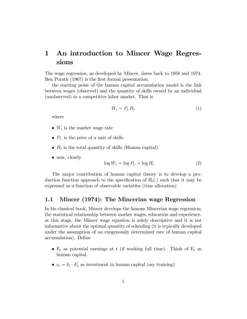
1 <strong>An</strong> <strong>introduction</strong> <strong>to</strong> <strong>Mincer</strong> <strong>Wage</strong> <strong>Regres</strong><strong>sions</strong><br />
The wage regression, as developed by <strong>Mincer</strong>, dates back <strong>to</strong> 1958 and 1974.<br />
Ben Porath (1967) is the first formal presentation.<br />
the starting point of the human capital accumulation model is the link<br />
between wages (observed) and the quantity of skills owned by an individual<br />
(unobserved) in a competitive labor market. That is<br />
where<br />
• Wt is the market wage rate<br />
Wt = Pt.Ht<br />
• Pt. is the price of a unit of skills<br />
• Ht is the <strong>to</strong>tal quantity of skills (Human capital)<br />
• now, clearly<br />
log Wt =logPt. +logHt<br />
The major contribution of human capital theory is <strong>to</strong> develop a production<br />
function approach <strong>to</strong> the specification of Ht(.) such that it may be<br />
expressed as a function of observable variables (time allocation)<br />
1.1 <strong>Mincer</strong> (1974): The <strong>Mincer</strong>ian wage <strong>Regres</strong>sion<br />
In his classical book, <strong>Mincer</strong> develops the famous <strong>Mincer</strong>ian wage regression;<br />
the statistical relationship between market wages, education and experience.<br />
at this stage, the <strong>Mincer</strong> wage equation is solely descriptive and it is not<br />
informative about the optimal quantity of schooling (it is typically developed<br />
under the assumption of an exogenously determined rate of human capital<br />
accumulation). Define<br />
• Et as potential earnings at t (if working full time). Think of Et as<br />
human capital.<br />
• ct = kt · Et as investment in human capital (say training)<br />
1<br />
(1)<br />
(2)
• kt is the amount of time (exogenous) devoted <strong>to</strong> training (kt =1when<br />
in school)<br />
• ρ t is the return <strong>to</strong> training (or schooling)<br />
Et+1 = Et + ct · ρ t = Et(1 + kt · ρ t) (3)<br />
• In general, starting from period 0 (earnings potential at 0 is E0)<br />
t−1<br />
Et =[<br />
Y<br />
(1 + kj · ρj)]E0 j=0<br />
now, divide the horizon in 2 periods (school and post schooling training)<br />
• ρ t = ρ s (in school)<br />
• ρ t = ρ 0 (in training activities)<br />
• clearly<br />
t−1<br />
Et =[<br />
Es =[(1+ρ s) s · E0<br />
Y<br />
(1 + kj · ρ0)](1 + ρs) s · E0<br />
j=s<br />
• taking logs of potential earnings, and noting that both ρ0 and ρs are<br />
small<br />
Xt−1<br />
(6)<br />
ln Et =lnE0 + s · ρ s + ρ 0 ·<br />
• the next steps are based on the willingness <strong>to</strong> introduce experience (X)<br />
in the expression. The trick is <strong>to</strong> specify kj(X) by imposing an exogenous<br />
rate of capital accumulation beyond school completion. Noting<br />
that at t=T-s=X<br />
j=s<br />
ln(w(s, x)) = α0 + ρ s · S + β 0 · X + β 1 · X 2<br />
which is the celebrated <strong>Mincer</strong> wage regression.<br />
• note that, returning <strong>to</strong> (.), the intercept term is now the product of the<br />
log skill price and the initial ability.<br />
2<br />
kj<br />
(4)<br />
(5)<br />
(7)
• ρ s acts as the ”return <strong>to</strong> schooling”<br />
• β 0/β 1 define the return <strong>to</strong> experience (and reflect concavity of the age<br />
earnings profile when β 1 is negative)<br />
• When (.) is augmented with race/ sex, then it may be used <strong>to</strong> study<br />
”discrimination”<br />
1.2 measuring the returns <strong>to</strong> schooling<br />
1.2.1 background<br />
Before describing the key aspects of the structural literature, it is useful <strong>to</strong><br />
survey some his<strong>to</strong>rical aspects. For the sake of the presentation, I consider<br />
two distinct periods. First, as the literature devoted <strong>to</strong> the return <strong>to</strong> schooling<br />
can hardly be distinguished from the <strong>Mincer</strong>ian wage regression, I review<br />
briefly the creation and the development of the <strong>Mincer</strong>ian wage regression<br />
model. A second period covers a large number of empirical studies that<br />
used Instrumental Variable (IV) techniques <strong>to</strong> infer the returns <strong>to</strong> schooling.<br />
These papers belong <strong>to</strong> an even larger set of empirical research using the<br />
“Natural Experiment” approach.<br />
The standard form of the <strong>Mincer</strong> wage regression is<br />
log Wt = wt = β 0 + β 1 · Schoolingt + β 2 · expt + β 3 · exp 2 t +εt<br />
where exp denotes accumulated labor market experience, β 0 is the sum of the<br />
rental price of human capital (in log) and the level of ability, and where β 1,β 2<br />
and β 3 are the parameters that represent the technology by which schooling<br />
and labor market experience are transformed in<strong>to</strong> skills.<br />
For a fixed (known) level of ability, the term εt represents a pure random<br />
shock affecting wages at a particular point in time. When (1) is fit<br />
<strong>to</strong> a cross-section of heterogenous individuals, the error term will typically<br />
be interpreted as unmeasured differences in innate ability. The assumptions<br />
of linearity in the error term and in accumulated schooling are ad hoc assumptions<br />
which are only based on statistical choices. As it will be clear<br />
later, these assumptions are not innocuous. Finally, the quadratic term in<br />
experience is meant <strong>to</strong> allow for the possible decline in post-schooling human<br />
capital acquisition.<br />
3<br />
(8)
The term “ability” should be unders<strong>to</strong>od as a time invariant level of skills<br />
that exists prior <strong>to</strong> the start of the human capital accumulation process and<br />
that affects labor market wages, even after controlling for acquired human<br />
capital. I refer <strong>to</strong> β 1 as the return <strong>to</strong> schooling. It designates the marginal<br />
effect of schooling in percentage on log wages (as opposed <strong>to</strong> the internal rate<br />
of return). If the effect of schooling is non-linear, the local return <strong>to</strong> schooling<br />
refers <strong>to</strong> the percentage wage increase per additional year of schooling. 1 The<br />
average return refers <strong>to</strong> the slope of the straight line between the intercept<br />
and the expected log wage at a given number of years of schooling. Finally,<br />
β 2 and β 3 are those that correspond <strong>to</strong> the return <strong>to</strong> experience.<br />
While the human capital literature has been generalized so <strong>to</strong> incorporate<br />
post schooling skill acquisition (say on-the-job training), it should be noted<br />
that the <strong>Mincer</strong>ian wage regression is a representation of the statistical relationship<br />
between wages and experience (given schooling) for an exogenously<br />
determined rate of on-the-job training. The <strong>Mincer</strong>ian wage regression disregards<br />
the endogeneity of post-schooling human capital accumulation and<br />
treats schooling and training symmetrically. More precisely, the <strong>Mincer</strong>ian<br />
approach usually ignores the possibility that schooling may change the onthe-job<br />
human capital accumulation process. 2 Statistically, these refinements<br />
would either require the joint modeling of schooling and training or the nonseparability<br />
between schooling and experience. As far as I know, these issues<br />
have not been addressed extensively in the empirical literature but are likely<br />
<strong>to</strong> be the object of research in a near future.<br />
1.2.2 The instrumental Variable (IV) Literature<br />
By the early 1970’s, the estimation of the returns <strong>to</strong> schooling using <strong>Mincer</strong>ian<br />
wage regres<strong>sions</strong> had become one of the most widely analyzed <strong>to</strong>pic in<br />
applied econometrics. In a famous survey, Griliches (1977) pointed out several<br />
econometric problems that arise in estimating the returns <strong>to</strong> schooling<br />
and, in particular, those pertaining <strong>to</strong> the measurement of both schooling<br />
and ability. Until then, substantial effort had been devoted <strong>to</strong> the estimation<br />
of the return <strong>to</strong> schooling with control variables measuring (or proxies<br />
of) unobserved ability. These measures are typically IQ tests or objects of a<br />
1 The terms local and marginal returns may be used interchangeably.<br />
2 In practice, this could arise if schooling affects traning opportunities or on-the-job<br />
search outcomes. Some related issues are mentioned in surveys such as those written by<br />
Willis (1986), Rosen (1984).<br />
4
similar nature, such as the Armed Forces qualifications (AFQT) tests. Those<br />
are most likely imperfect measures of labor market skills. Casual empiricism<br />
would reveal that AFQT scores (available in the popular National Longitudinal<br />
Survey of Youth) are more strongly correlated with schooling attainments<br />
than they are with wages 3<br />
More interestingly, Griliches recognized that the endogeneity of schooling<br />
deci<strong>sions</strong>, virtually ignored until then, was a serious issue which might<br />
have prevented economists <strong>to</strong> uncover the true causal effect of education on<br />
earnings. Subsequently, a wide range of empirical papers using instrumental<br />
variable (IV) techniques have been published. A large segment of this literature<br />
is based on “institutional features” of the education system. Card<br />
(2001 and 2002) presents an extensive survey of this literature and discuss<br />
the main conceptual issues within a unifying theoretical structure in which<br />
individuals compare the benefits of schooling with the costs of schooling born<br />
early in the life cycle. 4<br />
At the econometric level, the main issue may be illustrated by the following<br />
cross-sectional regression function<br />
wi = β 0 + β 1 · Schoolingi + η i = β 0 + β 1 · Si + η i<br />
Ignoring post-schooling labor market experience, it is clear that the discrepancy<br />
between OLS and IV estimates is a reflection of the correlation between<br />
schooling and unobserved ability (η i). A positive (negative) correlation is<br />
associated with a positive (negative) ability bias. In the IV literature, the<br />
ability bias is only indirectly investigated through the discrepancy between<br />
IV and OLS estimates, assuming that the linear model is correct. As we will<br />
see later, in structural models, the ability bias may be evaluated directly.<br />
With estimates of the utility of attending school and market ability, it may<br />
be obtained by simulation methods.<br />
E( ˆ β ols) =β + cov(η iSi)<br />
VarSi<br />
(9)<br />
(10)<br />
if cov(ηiSi) > 0 ability bias (positive) (11)<br />
if cov(ηiSi) > 0 ability bias (negative) (12)<br />
3 See Belzil and Hansen (2003).<br />
4 The model is intertemporal but is non-s<strong>to</strong>chastic. It borrows from becker (1967).<br />
5
To get around ability bias arguments, it is cus<strong>to</strong>mary <strong>to</strong> estimate the<br />
returns <strong>to</strong> schooling using IV methods. So let’s define an instrument Zi, such<br />
that<br />
The IV estima<strong>to</strong>r is such that<br />
Corr(Zi,Si) 6= 0 (13)<br />
Cor(Ziηi) = 0<br />
E( ˆ cov(log wi,Zi)<br />
βIV )=<br />
cov(SiZi) = β + cov(ηiZi) (14)<br />
cov(SiZi)<br />
inthecontextwhereSi (and Zi) is discrete, so di =1if individual i goes<br />
<strong>to</strong> school and 0 if not, we obtain a Wald estima<strong>to</strong>r<br />
E( ˆ β IV )= E(log wi | Zi =1− E(log wi | Zi =0)<br />
pr(di =1| Zi =1)− pr(di =1| Zi =0)<br />
(15)<br />
While a positive correlation between schooling and labor market ability<br />
is usually expected, Card (2001, 2002) reports that a large number of studies<br />
find that IV estimates exceed OLS estimates by a wide margin. 5<br />
ˆβ IV > ˆ βols (16)<br />
As of now, the IV literature retains two main explications for the high<br />
estimates.<br />
• First, the existence of significant measurement error in schooling may<br />
cause the OLS <strong>to</strong> be severely biased and underestimate the true return.<br />
My understanding of the literature is that the measurement error argument<br />
often advanced is typically set within a classical measurement<br />
error framework which ignores the correlation between schooling levels<br />
and the measurement error itself and also ignores the discrete nature<br />
of the schooling variable.<br />
• Second, in presence of heterogeneity in the returns (say when β 1<br />
varies across individuals), the IV estimate is inconsistent for the population<br />
average and the resulting estimate may reflectthereturnsof<br />
5 Estimates of the order of 15% per year of schooling are not uncommon.<br />
6
a sub-population only. Indeed, there is a large econometric literature<br />
concerned with the interpretation of IV estimates when the slopes are<br />
individual specific. 6 That is<br />
where<br />
which implies that<br />
log wi = β 0 + β i · Si + η i<br />
β 1i = ¯ β 1 + η β<br />
i<br />
log wi = β 0 + ¯ β 1 · Si + η β<br />
i · Si + η i = β 0 + ¯ β 1 · Si + η ∗ i<br />
(17)<br />
(18)<br />
(19)<br />
where<br />
η ∗ i = η β<br />
i · Si + ηi. (20)<br />
Clearly, ˆ βIV is inconsistent for ¯ β1. why? Can Zi ⊥ η∗ i ? only if Si ⊥ η β<br />
i . In<br />
theory, optimal schooling (Si) is function of η β<br />
i .<br />
When the wage regression is given by (.). we refer <strong>to</strong> a correlated<br />
random coefficient model (again randomness refers <strong>to</strong> the dispersion in<br />
β1i so it is not random from the perspective of the agent.<br />
The intuition for the failure of IV is simple; in such a framework, individual<br />
reactions induced by Zi are heterogeneous, so the parameter arising<br />
from IV estimation is only valid for those who changed status following the<br />
experiment. So, the IV estima<strong>to</strong>r is only valid for a sub-population (it is not<br />
¯β 1)<br />
1.2.3 Other Problems with the IV literature<br />
Regardless of measurement error and neglected population heterogeneity, the<br />
IV literature may be criticized for three main reasons.<br />
• First, Instrumental variables (IV) techniques may be applied in a context<br />
where the instrument is only weakly correlated with schooling<br />
attainments (Staiger and S<strong>to</strong>ck, 1997). Indeed, before the late 90’s,<br />
most empirical researchers concentrated their efforts on finding an instrument<br />
uncorrelated with neglected ability, but the power of the instrument<br />
chosen was practically never investigated. In the presence of<br />
6 For a statistial discussion, see Imbens and <strong>An</strong>grist (1994).<br />
7
weak instruments, reported estimates may be at best imprecise and, at<br />
worst, seriously biased (or inconsistent). As a consequence, the validity<br />
of very high returns <strong>to</strong> schooling, reported in a simple regression framework,<br />
should be seriously questioned. two cases are worth considered:<br />
cov(SiZi) ≈ 0 (cov(η iZi =0)→ σ 2 (Z 0 D) −1 Z 0 Z(Z 0 D) −1 →∞ (21)<br />
cov(SiZi) ≈ 0 (cov(ηiZi ≈ 0) → cov(ηiZi) →∞(bias) (22)<br />
cov(SiZi)<br />
• Second, when IV techniques are chosen, the log wage regression is usually<br />
assumed <strong>to</strong> be linear in schooling and, perhaps, quadratic in experience.<br />
However, there is no obvious reason <strong>to</strong> presume that the local<br />
returns <strong>to</strong> schooling are independent of grade level. As individuals with<br />
lower taste for schooling tend <strong>to</strong> s<strong>to</strong>p school earlier, OLS (or IV) estimates<br />
of the return <strong>to</strong> schooling, which impose equality between local<br />
and average returns at all levels of schooling, will be strongly affected<br />
by the relative frequencies of individuals with high and low taste for<br />
schooling. 7 More precisely, if there are large differences in local returns<br />
between various grade levels, the OLS estimate (measuring an average<br />
log wage increment per year of schooling) will tend <strong>to</strong> be biased <strong>to</strong>ward<br />
the local returns at schooling attainments that are the most common<br />
inthesampledata.<br />
wi = β 0 + ϕ(Schoolingi)+η i<br />
(23)<br />
• Finally, the IV literature rarely addresses labor market experience per<br />
se. This is surprising as labor market experience represents a key substitute<br />
<strong>to</strong> schooling as a mean for enhancing life cycle wages. A survey<br />
of the IV literature reveals that practically no paper presents a joint<br />
estimation of the returns <strong>to</strong> schooling and experience. A quick glance<br />
at the <strong>Mincer</strong>ian wage regression (2) reveals that without controls for<br />
individual differences in accumulated post-schooling human capital, it<br />
is difficult <strong>to</strong> give a interpretation <strong>to</strong> the discrepancy between OLS and<br />
7 This issue is sometimes referred <strong>to</strong> as the Discount Rate bias.<br />
8
IV estimates. 8 To see this, return <strong>to</strong> the simple homogenous return<br />
case β 1i = β 1 for everyone.<br />
wi = β 0 + β 1 · Si + δ · PSHCi + η i = β 0 + β i · Si + η ∗ i<br />
(24)<br />
where PSHCi denotes all post schooling investment activities (training,<br />
search...) and<br />
η ∗ i = δ · PSHCi + η i. (25)<br />
Now reconsider estimating (.), this implies that for Zi <strong>to</strong> be valid (if wages<br />
are measured after entrance in the labor market), the following must be true<br />
Zi ⊥ η ∗ i<br />
(26)<br />
but, in general, this cannot be true because Zi ⊥ PSHCi cannot be<br />
true (think about season of birth, and what happens if you lose one year of<br />
human capital accumulation). That if if, for instance, one individual loses<br />
oneyearthenhe/shemayreactbyinvestinginpostschoolingtraining,search<br />
activities and any other wage enhancing activities (Rosenzweig and Wolpin,<br />
2000, Journal of Economic Literature).<br />
8Many issues related <strong>to</strong> the endogeneity of work experience are discussed in Rosenzweig<br />
and Wolpin (2000)<br />
9