november 2010 volume 1 number 2 - Advances in Electronics and ...

NOVEMBER 2010 VOLUME 1 NUMBER 2

Journal Editorial Board 

KRZYSZTOF WESOŁOWSKI, Editor-in-Chief 

Poznan University of Technology 

Piotrowo 3A, 60-965 Poznań, Poland 

krzysztof.wesolowski@et.put.poznan.pl 

WOJCIECH BANDURSKI 


ANNA DOMAŃSKA 


MACIEJ STASIAK 


Advisory Board 

FLAVIO CANAVERO 

Politecnico di Torino 

Italy 

LAJOS HANZO 

University of Southampton 

UK 

MACIEJ OGORZAŁEK 

AGH Technical University 

Jagiellonian University 

Cracow, Poland 

Cover design Barbara Wesołowska 

ANNA PAWLACZYK, Secretary 



anna.pawlaczyk@et.put.poznan.pl 

HANNA BOGUCKA 


MAREK DOMAŃSKI 


RYSZARD STASIŃSKI 


TADEUSZ CZACHÓRSKI 

Polish Academy of Science 

Institute of Theretical and Applied 

Informatics 

Gliwice, Poland 

MICHAEL LOGOTHETIS 

University of Patras 

Greece 

JOHN G. PROAKIS 

University of California 

San Diego, USA 

c○ Copyright by POZNAN UNIVERSITY OF TECHNOLOGY, Poznań, Poland, 2010 

Edition based on ready-to-print materials submitted by authors 

Materials published without further editing at the responsibility of the authors 

ISBN 978-83-7143-899-8 

ISSN 2081-8580 

PUBLISHING HOUSE OF POZNAN UNIVERSITY OF TECHNOLOGY 

60-965 Poznań, pl. M. Skłodowskiej-Curie 2 

tel. +48 (61) 6653516, fax +48 (61) 6653583 

e-mail: office_ed@put.poznan.pl 

www.ed.put.poznan.pl 

ADRIAN LANGOWSKI, Technical Editor 



adrian.langowski@et.put.poznan.pl 

ANDRZEJ DOBROGOWSKI 


WOJCIECH KABACIŃSKI 


PAWEŁ SZULAKIEWICZ 


PIERRE DUHAMEL 

CNRS - Supélec 

France 

JÓZEF MODELSKI 

Warsaw University of Technology 

Poland 

RALF SCHÄFER 

Fraunhofer Heinrich-Hertz-Institut 

Berlin, Germany 

ADVANCES IN ELECTRONICS AND TELECOMMUNICATIONS is a peer-reviewed journal published at Poznań University of Technology, Faculty 

of Electronics and Telecommunications. It publishes scientific papers addressing crucial issues in the area of contemporary electronics and 

telecommunications. Detailed information about the journal can be found at: www.advances.et.put.poznan.pl.

NOVEMBER 2010 VOLUME 1 NUMBER 2 

Radio Communication Series: 

Poznań Telecommunications Workshop 

Issue Editor: Paweł Szulakiewicz 

Note from the Issue Editor 

Paweł Szulakiewicz . . . . . . . . . . . . . . . . . . . . . . . . . . . . . . . . . . . . . . . . . . . . . . . . . . . . 1 

Wireless Systems and Networks 

Multipurpose Radio for Railways.Construction and Applications 

J. Kasperek, A. Nikoniuk, and P. Rajda . . . . . . . . . . . . . . . . . . . . . . . . . . . . . . . . . . . . . . . . . 3 

Simulation Study of the IEEE 802.15.4 Standard Low Rate Wireless Personal Area Networks 

D. Ko´scielnik and J. St˛epień . . . . . . . . . . . . . . . . . . . . . . . . . . . . . . . . . . . . . . . . . . . . . . . 7 

Diversity and Multiplexing Techniques 

M. Krasicki . . . . . . . . . . . . . . . . . . . . . . . . . . . . . . . . . . . . . . . . . . . . . . . . . . . . . . . . 12 

Spectral Analysis of Boosted Space-Time Diversity Scheme 

M. Krasicki . . . . . . . . . . . . . . . . . . . . . . . . . . . . . . . . . . . . . . . . . . . . . . . . . . . . . . . . 17 

Krylov Subspace Methods in Application to WCDMA Network Optimization 

R. Zdunek and M. Nawrocki . . . . . . . . . . . . . . . . . . . . . . . . . . . . . . . . . . . . . . . . . . . . . . . 22 

Networks 

Streaming Video over TFRC with Linear Throughput Equation 

A. Chodorek and R. R. Chodorek . . . . . . . . . . . . . . . . . . . . . . . . . . . . . . . . . . . . . . . . . . . . 26 

Simulation model for evaluation of packet sequence changed order of stream in DiffServ network 

M. Czarkowski and S. Kaczmarek . . . . . . . . . . . . . . . . . . . . . . . . . . . . . . . . . . . . . . . . . . . . 30

Packet dispatching schemes supporting uniform and nonuniform traffic distribution patterns in msm clos-network 

switches 

J. Kleban . . . . . . . . . . . . . . . . . . . . . . . . . . . . . . . . . . . . . . . . . . . . . . . . . . . . . . . . . 35 

Time and Synchronization 

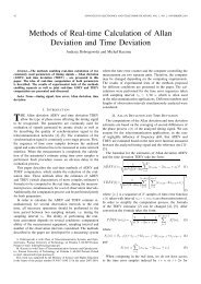
Methods of Real-Time Calculation of Allan Deviation and Time Deviation 

A. Dobrogowski and M. Kasznia . . . . . . . . . . . . . . . . . . . . . . . . . . . . . . . . . . . . . . . . . . . . . 42 

Application of Vernier Interpolation for Digital Time Error Measurement 

K. Lange and M. Kasznia . . . . . . . . . . . . . . . . . . . . . . . . . . . . . . . . . . . . . . . . . . . . . . . . 47 

Communication Theory 

Improving Statistical Properties of Number Sequences Generated by Multiplicative Congruential Pseudorandom 

Generator 

M. Jessa . . . . . . . . . . . . . . . . . . . . . . . . . . . . . . . . . . . . . . . . . . . . . . . . . . . . . . . . . . 51 

New Tailbiting Convolutional Codes over Rings 

P. Remlein and D. Szłapka . . . . . . . . . . . . . . . . . . . . . . . . . . . . . . . . . . . . . . . . . . . . . . . . 55 

Fiber Optics 

Modeling Step Index Fiber to Soliton Propagation 

T. Kaczmarek . . . . . . . . . . . . . . . . . . . . . . . . . . . . . . . . . . . . . . . . . . . . . . . . . . . . . . . 59 

Are Carrier Transport Effects Important for Chirp Modeling of Quantum-Well Lasers? 

P. Krehlik . . . . . . . . . . . . . . . . . . . . . . . . . . . . . . . . . . . . . . . . . . . . . . . . . . . . . . . . . 63 

Precise Measurements of Highly Attenuated Optical Eye Diagrams 

P. Krehlik, Ł. ´Sliwczyński, and G. Sikorski . . . . . . . . . . . . . . . . . . . . . . . . . . . . . . . . . . . . . . . 67 

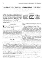
Bit Error Rate Tester for 10 Gb/s Fibre Optic Link 

Ł. ´Sliwczyński and P. Krehlik . . . . . . . . . . . . . . . . . . . . . . . . . . . . . . . . . . . . . . . . . . . . . . 70

ADVANCES IN ELECTRONICS AND TELECOMMUNICATIONS, VOL. 1, NO. 2, NOVEMBER 2010 1 

Note from the Issue Editor 

The second issue of Advances in Electronics and Telecommunications 

contains sixteen selected papers presented at the last two editions 

of Poznań Telecommunications Workshop: PWT 2007 and 2008 

(www.pwt.et.put.poznan.pl). The conference held annually in Poznań at 

the beginning of December is devoted to topics concerning research and 

education in telecommunications, electronics, and related fields. These most 

important areas of Information and Communication Technologies focus the 

attention of the workshop participants, who are mainly young researchers 

and PhD students from Polish universities of technology. 

The PWT workshops in Poznań have become a forum for developing a 

wide range of professional relationships. Both the presentations of research 

results and the discussions that follow provide the young authors with 

valuable opportunities to interact with more experienced scientists, industry 

professionals and innovators in the fields of their particular interests. 

We hope that the selection of PWT papers included in this issue of 

Advances proves to be interesting to the readers. 

The presented papers are divided into the following five groups: Wireless Systems and Networks, Networks, 

Time and Synchronization, Communication Theory, Fiber Optics. 

We would like the Advances journal and the Poznań Telecommunications Workshop to bridge the gap between 

research and development, and engineering and implementation. Our readers will judge how far we are from that 

goal. 

Paweł Szulakiewicz 

Issue Editor


Multipurpose Radio for Railways. Construction and 

Applications 

Abstract—This paper provides information on the construction 

and presents experience from the “Koliber” project: a modern 

multipurpose radio system for railways. The radio equipment is 

produced by Radionika Ltd., and was designed in cooperation 

with Department of Electronics, AGH University of Science and 

Technology. Discussed here are system architecture,technical and 

functional parameters, and innovative radio system applications 

possible thanks to its innovatory construction. 

Index Terms—VHF railway radio, GSM-R 

I. INTRODUCTION 

Jerzy Kasperek, Andrzej Nikoniuk, and Paweł Rajda 

“ 

KOLIBER” is a modern solution for radio communication, 

designed exclusively for railway needs. The device 

works as a mobile set in double-cabinlocomotivesof all types 

and in any other rail vehicles. The stationary version of the 

radio is intended to work as a base station, operated by the 

railway dispatcher. 

The device provides radio connections of all types in radio 

networksoperatedby railway companies,using VHF 150MHz 

band. The device provides a specific signaling used in Polish 

railways: tone selected calls (Zew1, Zew3) and emergency 

train stop protocol [1], [2]. Among the mandatory functions 

presented above, the solution offers more advanced functions 

available in contemporary radio communication. In particular, 

the device enables a range of functions including selective 

call signaling (SelCall), CTCSS/DCS encoding and decoding, 

modem data transmission, and GPS navigation. 

Furthermore, the architecture and technology of the equipment 

allow also using the device in other communication 

network standards (including GSM and GSM-R). Besides the 

obvious economic benefits (single device supporting multiple 

communication systems), this solution significantly simplifies 

the operationof radio for railway vehicle driversand dispatchers. 

“Koliber” is a solution that not only serves the needs 

of current users of the railway network but also ensures the 

operationofequipmentaftermodernizationofthe networkand 

during switching to a new digital communication standard. 

The device is fully compatible with mounting and connectors 

currently used in vehicles and dispatcher desks. The dimensionsandsolutionsofthedeviceweredesignedtoenablequick 

assemblyandsetupwithuseoftheexistingwiringandfixtures. 

II. RADIO SET ARCHITECTURE 

Fig. 1 presents the architecture of the radio set version 

designed for the double-cabin locomotives. Both cabins are 

Fig. 1. “Koliber” radio system architecture. 

equipped with a manipulator (DMI – Driver Machine Interface). 

Each DMI is connected with an intelligent switch 

module which commutes signals to the radio module. The 

switchmodulemayoptionallybeequippedwithaGSMengine 

to carry on voice communication through the mobile phone 

network of any operator and/or to transmit GPRS messages, 

including the status, geographical coordinates, and parameters 

of the locomotive (e.g. the consumption of fuel in combustion 

locomotives). 

The entire set is powered through a universal DC/DC 

converter,workingwithinawiderangeofvoltage(15...212V). 

Single-cabin locomotive sets have only one DMI mounted, 

while stationary sets feature an AC/DC power supply mounted 

instead of the DC/DC converter. Moreover, the open architecture 

of the device enables integration of any ready-to-use 

GSM-R external modules [3]. To date, successful integration 

with certified PortBox Ultralight GSM-R module of HFWK 

(formerly Kapsch) was performed. 

III. DRIVER-MACHINE INTERFACE MODULE 

The DMI (Driver-Machine Interface) module performs the 

role of the user’s interface radio. Its main operationalelements 

include: 

• high resolution graphic LCD display with backlight, 

• contextually illuminated numeric and functional keypad, 

• “RadioStop” button being a part of the emergency train 

stop system, 

• set of signaling LEDs, 

• microphone with the PTT (Push To Talk) key, 

• speaker, 

• 1-Wire interface for identification/authentication. 

The block diagram of the DMI module is presented in 

Fig. 2. It is a typical microcontroller application based on 

a 8-bit Atmel RISC ATmega128 device. The DMI features a

4 ADVANCES IN ELECTRONICS AND TELECOMMUNICATIONS, VOL. 1, NO. 2, NOVEMBER 2010 

Fig. 2. Driver Machine Interface block diagram. 

large and clear graphic LCD display unit with resolution of 

240×64 pixels to present the current state of the whole radio 

set. The display presents also contextual description of the 

keyboard functions. The meaning of particular keys depends 

on the menu selected, and contextual illumination facilitates 

their operation further. 1-Wire contact devices are used for 

access authorization and radio operator log-in & log-out. 

Communication with other modules of the set is performed 

via RS422 bus, while the radio voice is sent as analogue. 

IV. SWITCH MODULE 

The primary task of the switch module is commutation of 

signals between the radio module and the active DMI in one 

of the two locomotive cabins. This module was designed and 

developed as a natural replacement for the mechanical switch 

used before in most locomotives in Poland [4]. The switch 

module can optionally be equipped with the GSM Motorola 

G24 engine. This solution enables concurrent usage of the 

audio and data GSM services parallel to standard work in the 

VHF band.This allows using emergencycalls as well as SMS. 

What is more, once a GPS module has been installed, it 

is also possible to transfer train location data via the GPRS 

data link. The GPRS network link is a convenient medium 

for transmission of all kinds of status messages between the 

driver and the stationary rail service. The switch module 

architecture is presented in Fig. 3. It uses an ATmega128 

microcontrollerasthemainprocessor.Duetothelargenumber 

of serial port controlled modules, a quadruple UART is used. 

This module can also be used in stand alone mode, e.g. 

as an intelligent GPRS modem for localization systems and 

for various data acquisition solutions. To enable its operation 

even after the locomotive’s on-board supply failure (or while 

locomotive is being moved), the module is equipped with a 

power management system with a high capacity battery cell. 

V. RADIO MODULE 

The radio module contains the main execution unit for the 

whole set. The Tait TM8100 VHF transceiver module is used 

as the RF engine, and all the other functions – including audio 

signaling, data transmission and voice recording – are carried 

out by a dedicated unit control module. 

Fig. 3. Switch module block diagram. 

Fig. 4. Radio system architecture. 

Below listed are the parameters of the radio module: 

• 134-174 MHz frequency VHF band, 

• 256 radio channels, 

• scanning, 

• programmable channels frequency, RF power, and channel 

spacing, 

• generation and detection of the emergency “Radiostop” 

signal, 

• generation and detection of sub-audio CTCSS/DCS signals 

and selective call audio signaling, 

• 1200/2400bps modem data transmission, 

• call party ID generation and detection, 

• radio voice and system event recording with optional 

external recording channel, 

• GPS internal module option, external DCF module port, 

• RTC clock. 

The Fig. 4 presents the block diagram of the radio module 

architecture. The TM8100 VHF transceiver is controlled by 

a serial port with the Tait company proprietary command 

protocol. All RF parameters are controlled by respective 

appropriate software commands. A dedicated audio processor

KASPEREK et al.: MULTIPURPOSE RADIO FOR RAILWAYS.CONSTRUCTION AND APPLICATIONS 5 

Fig. 5. “Koliber” GPS System architecture. 

Fig. 6. “Qguar Qpilot” localization window. 

CMX7041 chip from CML is used for all audio and sub-audio 

signaling,andalso formodemtransmission.InPoland,thecall 

party ID signals are transmitted as modem messages. 

The radio module is controlled by the same type of microcontroller(ATmega128fromAtmel).However,duetoasignificant 

need of hardwareresources, the remainingmodule architecture 

is implemented in 200k gates FPGA Spartan3 device 

from Xilinx. The main subsystem implemented in FPGA is 

the Secure Digital flash memorycard host controller.SD cards 

are used as the archive repository for voice and event records. 

To enable quick archive content reading without removing the 

SD card, an SD controller was designed to work in a highspeed 

parallel (4-bit data bus) mode with troughput exceeding 

10MB/s. In addition, the FPGA implements an interface to a 

USB 2.0 controller, two UARTs (one for communication with 

the TM8100 VHF transceiver and the other for the service), 

two CVSD codec drivers (one for recording audio from the 

radio set; i.e. VHF GSM calls, the other for an optional 

externalvoicerecorder),externaldatamemoryinterfaceforthe 

microcontroller, and the authentication subsystem based on a 

hardware implementationof Blowfish cryptographicalgorithm 

with external “1-Wire” ID device. 

The module uses a small backup battery for the real-time 

clock device. Time synchronization is provided by the GPS 

engine, which – in the case of desktop solutions – may be 

replaced with an external DCF77 receiver. 

Fig. 7. Real-time locomotive cockpit visualization. 

Fig. 8. Architecture of DSR radio dispatcher system. 

VI. SYSTEM FIRMWARE 

Microcontrollers software was written in C language in the 

IAR AVR environment, and the FPGA project was created 

with VHDL. 

The intelligent switch module with GPRS option uses UIP 

TCP/IP freeware stack [5]. The web server and client ensure 

HTTP support for the “post” and “get” commands. When 

the external monitoring device is connected, one can use 

the proprietary protocol to query the module for numerous 

parameters of the locomotive and localization. There is also 

an option to remotely change any EEPROM configuration 

memory content, e.g. the APN name and other GPRS network 

connection parameters.


Fig. 9. GUI of DSR radio dispatcher system. 

Fig. 10. GIS RSSI data report. 

The AVR bootloader feature may be used to change any 

module microcontroller program memory and/or the FPGA 

configuration memory content, which facilitates firmware upgrades. 

All radio parameters can be set up using a dedicated 

software connected to the DMI module service RS232 port. 

VII. APPLICATIONS AND EXPERIENCES 

Based on the referred solution, some interesting applications 

of the radio set have been implemented. Their number 

includes: 

• train localization and locomotive parameters monitoring 

system, 

• DSR dispatcher system – remotely controlled VHF base 

station sets for railway main tracks, 

• G.sHDSL modem for the radio remote controll, 

• GIS RSSI measurement system for railway tracks. 

Presented below is a selection of screens and diagrams of the 

aplications mentioned. 

Fig. 5 presents “Qguar Qpilot” fleet management system 

architecture from Quantum Software S.A. The “Koliber” radio 

set sends localization data from GPS via the GPRS link to the 

company’s APN GSM infrastracture. Fig. 6 presents a sample 

GUI window from the application. 

Fig. 7 presents real time visualization of the locomotive 

parameters from the “Koliber” switch module, connected to 

the CL400 module of the locomotive monitoring unit (manufactured 

by ZEPWN). 

Fig. 9 presents an architecture of the DSR dispatcher radio 

system,whichconsistsofseveralradiobasestationscontrolled 

by dispatchers from the Local Control Center. Each base 

station includes up to 4 radios, along with a service DMI 

module and a control unit. Base stations are connected with 

Local Control Center by SDH based E1 links, forming a star 

structure. 

Fig. 10 presents example results of the radio signal strength 

measurement system done with the “Koliber” set on one of 

the main Polish rail tracks. 

VIII. CONCLUSION 

A few years of using the “Koliber” system in railway 

radio networks allow the conclusion that the design based 

on a simple 8-bit microcontroller, equipped with few external 

devices for dedicated functions, is fully justified. The design 

was verified by approvedindustrial bodies, positively tested in 

the real consumer world, and opened many new application 

fields. 

REFERENCES 

[1] “R-12 instrukcja o u˙zytkowaniu urz˛ adzeń radioł˛ aczno´sci poci˛ agowej na 

pkp,” Biuletyn PKP, zał˛ acznik do nr 25 z dn. 18.12.1992, poz 102, (in 

Polish). 

[2] E36 Instrukcja o organizacji i u˙zytkowaniu sieci urzadzeń ˛ radiołaczno´sci ˛ 

w przedsi˛ebiorstwie państwowym PKP, (in Polish). 

[3] “GSM-R Procurement Guide,” [online], Feb. 2007, www.uic.asso.fr. 

[4] R. Markowski, “Stan obecny radioł˛ aczno´sci na pkp – problemy i wyzwania,” 

in Proc. of Radiołaczno´sć ˛ w kolejnictwie wczoraj - dzi´s - jutro, 

Telekomunikacja Kolejowa Warszawa, Sep. 2003, (in Polish). 

[5] A. Dunkels, “Full TCP/IP for 8-Bit Architectures,” in Proc. of 1st 

International Conference on Mobile Applications, Systems and Services, 

MOBISYS, San Francisco, May 2003. 

Jerzy Kasperek, Paweł J. Rajda (kasperek@agh.edu.pl, pjrajda@agh.edu.pl) 

– Department of Electronics, AGH University of Science and Technology, 

30-059 Kraków, Al. Mickiewicza 30. Interest areas: digital design, hardware 

description languages, programmable logic and microcontroller applications, 

hardware accelerated signal processing, custom computing machines. 

Andrzej Nikoniuk (andrzej.nikoniuk@radionika.com) – Radionika sp. z o.o., 

30-003 Kraków, ul. Lubelska 14-18, Interest areas: railway radiocommunication 

systems design, business development managing.


Simulation Study of the IEEE 802.15.4 Standard 

Low Rate Wireless Personal Area Networks 

Abstract—This article presents a description of the simulation 

study of the low rate wireless personal area networks, defined 

by the IEEE 802.15.4 standard. The obtained results make 

it available to evaluate the effective transmission rate of a 

transmission channel,theresistance tothephenomenonof hidden 

station as well as the sensibility to the problem of exposed node. 

Index Terms—Exposed station, hidden station, low rate wireless 

area network 


THE IEEE 802.15.4 standard was created in 2003, and its 

current form results from the modifications introduced 

three years later. The specification defines the physical layer 

(PHY), the medium access control sublayer (MAC), as well 

as the principle of their interaction with the higher layers. 

The LR-WPAN are characterized by very low energy consumption, 

simplicity of their structure making it possible to 

implementthe transmissionprotocolon8-bit microcontrollers, 

as well as low costs of receiving and transmitting equipment. 

LR-WPAN aredesignedto beusedin differentindustrial,agricultural 

and alarm systems, building automatics, monitoring, 

interactive toys and in particular in wireless sensor networks 

(WSN). 

The bit rate of the IEEE 802.15.4 network can be equal to: 

20 kb/s, 40 kb/s, 100 kb/s or 250 kb/s. The nodes realize the 

transmission in a discontinuous way, trying to remain for the 

longest possible time in inactive mode – this make it possible 

to achievelow energyconsumption.The radiated poweris less 

than 1 mW, and the transmission range, characteristic for the 

personal operating space class solutions (POS), equals 10 m. 

The IEEE 802.15.4 standard offers a high capacity of the 

system and a very fast identification of equipment appearing 

in its range. The number of operating nodes can equal 216 or 

264 , dependent on the length of addresses, whereas in general 

the time of registration of a new node does not exceed 30 ms. 

Moreover, a precious advantage is the automatic modification 

of connections with moving equipment. 

The IEEE 802.15.4 standard offers two ways of transmission: 

in non-synchronized (non-beacon) and in synchronized 

(bacon enabled) mode. The first one defines only a 

contention access, using a simple mechanism permitting to 

identify the channel state and avoid collisions – unslotted- 

CSMA/CA (carriersense,multipleaccesswithcollisionavoidance). 

In the second method a less developed, slotted contention 

protocol has been implemented – slotted-CSMA/CA, 

as well as a no-collision access mechanism. 

Dariusz Ko´scielnik and Jacek St˛epień 

II. SIMULATION TESTS OF THE CONTENTION PROTOCOL 

The main objective of the tests of the contention protocol 

implemented in the IEEE 802.15.4 network was to define its 

efficiency and resistance to the appearance of hidden stations 

or exposed stations in the system, named also blocked nodes. 

The simulation was realized using a NetSim package created 

in the Department of Electronics, AGH University of Science 

and Technology. The NetSim software has been written in 

C++language.Thepackageusesanevent-planningtechnology 

(event queue). Its mechanisms permit to correctly render 

the reciprocal time interrelations existing between several 

simultaneous processes. The importance of simulated time as 

well as the number of stages of the tested processes can be 

dynamically adapted to the following factors: the character of 

the observed events, the momentary importance of the offered 

traffic, the size of the tested system as well as the required 

precision of obtained results. 

In the further part of this work we have presented the 

results of tests relating to the evaluation of the efficiency 

of CSMA/CA protocol implemented in non-synchronized and 

synchronized LR-WPAN network. In all the studied cases the 

assumptions are as follows: transmission rate of 250 kb/s, the 

DATAframestransmitdatafieldswithmaximalpermittedsize, 

the node emitters are equipped with buffers with a capacity 

of 50 packets and every successful transaction ends with an 

ACK frame. Moreover, we have admitted a two-ray ground 

propagation model, meaning that the nodes located within 

the emitter range correctly receive its transmission with a 

probability equal to 1. The other stations do not hear the 

transmission – their probability of packet reception equals 0. 

In the simulation model, we did not take into consideration 

the possible impact of any external interference that might 

decreasethe efficiencyof the transmission.Therefore,the only 

possible cause of unsuccessful transfer can be a collision. 

A. Effective transmission rate of the transmission channel 

The effective transmission rate of the transmission channel 

indicates a maximumnumber of user’s data transmitted within 

a time unit [1]. Usually, the value of this parameter is largely 

different from the used transmission rate, because of the 

overhead introduced by the second and first layers as well 

as because of the inactivity periods related to the duration of 

transmission delay times and the testing of channel occupation 

during the contention. 

For the identification of effective transmission rate of the 

system, we have used a model containing two nodes, one 

of them working as coordinator. The transmission is realized


only in one direction – towards the coordinator.Therefore, the 

network is free of collisions and the intensity of the operated 

traffic is the maximal possible. 

The results obtained for both network operation modes 

(non-synchronized and synchronized) are summarized in 

Fig. 1. The effective transmission rate in the non-synchronized 

mode equals to 116 kb/s, corresponding to the utilization of 

46 % of the channel operation time. The remaining transmission 

rate of the system is absorbed by the transmission 

overhead and by the dead periods, related to the random 

delay of the moment starting transmission. The effective 

transmission rate of the synchronized network is even worse 

and equals about 98 kb/s, corresponding to 39 % of the 

assumed transmission rate. The supplementary band losses 

result from the necessity of the periodical transmission of 

BEACON frame, the increasing of the channel occupation 

test, the increasing of the contention window size and the 

non-utilization of the last fragment of the superframe, which 

remains empty because the transmitting node cannot manage 

to fit the entire transaction in it. The average length of this 

section corresponds to the half of the transaction time. 

The Fig. 1.b presents the relation between the coefficient of 

delivered packets and the intensity of the offered traffic. The 

losses of frames appear only during the overloading of the 

system. The superiority of the traffic offered over the traffic 

operated leads to the overfilling of the emitter’s queue and the 

resulting refusal of a certain part of the requests. 

Thesame modelofthesystem, loadedwith a trafficdirected 

inasymmetricalwaytobothnodes,makesitpossibletodefine 

the influence of the bidirectionaltransmission for the available 

transmission rate of the network. The obtained results are 

summarized in Fig. 2. Their values are not significantly worse, 

evenif it couldseemthatthe nodesshouldinitiateacontention 

concerning the access to the common channel, leading to 

collisions. In the LR-WPAN, the transactions realized in 

both directions are initiated by a single slave station, so any 

contention is excluded. The decrease in the transmission rate 

of the transmission channel results from a worse efficiency 

of transmission directed towards the slave node. Any such 

transaction must start with the transmission of REQUEST and 

ACK frames [1], increasing its duration. 

The coefficient of delivered packets, defined for the discussed 

configuration, has slightly changed because of the 

decrease in the transmission rate of the network (Fig. 2.b). 

The form of both curves remains identical, confirming a total 

operation of the requests directed toward a system free of 

overloading. 

B. Influence of a hidden station on the transmission rate of 

the system 

The collisions caused by hidden stations are much more 

troublesome for the system than those resulting from the 

contention for the access to the radio channel. A long time 

of emission of a single frame significantly increases the 

probability of generating a new request directed to the hidden 

station in this period [2]. Its immediate realization will disturb 

the transactionbeing alreadyin progresswith the distant node. 

Fig. 1. Unidirectional transmission in a system consisting of two nodes: a) 

intensity of the operated traffic, b) coefficient of delivered packets 

Studying the influence of the presence of a hidden station 

on the operation of the LR-WPAN network, we have used 

the model presented in Fig. 3. A centrally placed coordinator 

works with two slave nodes, located out of their reciprocal 

range. The entire offered traffic is evenly divided between 

slave stations, which direct their transfers exclusively to the 

coordinator. 

The results of simulation tests, summarized in Fig. 4, 

indicate a radical decrease in the transmission rate of the 

system – for both transmission modes it equals only 23 % of 

the effective channel transmission rate. Moreover, the network 

works with the efficiency close to maximal only in certain, 

relatively narrow interval of the intensity of the offered traffic. 

A further increase in the number of requests results in an 

important worsening of the quality of their servicing and 

in system overloading. The shape of obtained characteristics 

correspondsto the panic curve,defining the operationof many 

systems with collision access. 

The reason of the decrease in the network transmission rate 

– when the intensity of the offered traffic exceeds of a given 

threshold value – is the increase in the channel occupation 

time, favorable to the appearance of collisions with the hidden 

stations. The retransmissions activated by both nodes increase 

in an artificial way the intensity of requests directed towards 

the system, leading to its overloading. It is worth mentioning

KO´SCIELNIK AND STEPIEŃ: ˛ SIMULATION STUDY OF THE IEEE 802.15.4 STANDARD LOW RATE WIRELESS PERSONAL AREA NETWORKS 9 

Fig. 2. Bidirectional transmission in a system consisting of two nodes: a) 


Fig. 3. Model of a system containing hidden stations 

that in congestion conditions the transmission rate of a nonsynchronized 

network decreases to zero, whereas a synchronized 

system always guarantees a certain minimal level of 

servicing the transmission requests. Such an advantage is a 

side effect of the algorithm realized by the node of the LR- 

WPAN network, verifying before the start of each transaction 

if its duration does not exceed the limits of the finishing 

superframe. Thanks to that, the hidden station rarely disturbs 

the last transmission that can fit into the superframe. 

The defined characteristics of the coefficient of delivered 

packets (Fig. 4.b) indicate that the loss of frames appears 

even with a very little intensity of the offered traffic. The 

reason is the cancellation of further retransmissions of these 

packets, not delivered with a pre-defined admissible number 

of attempts. As the intensity of the requests increases, this 

phenomenon appears more and more often. In an overloaded 

system, the queues of single emitters become overfilled and a 

Fig. 4. Unidirectional transmission in a system containing hidden stations: 

a) intensity of the operated traffic, b) coefficient of delivered pa 

more significant part of the offered traffic is refused. 

The objective of successive series of tests consisted in 

verifying the influence of the hidden station on the node 

located in the range of its signal. In the system presented 

in Fig. 3 this function is assumed by the coordinator. We 

should remind that the transactions of the coordinator are 

initialized by other nodes of the cluster, strongly influenced 

by the presence of the hidden station. Based on this, we can 

presume that the hidden station will also disturb the servicing 

of requests directed towards the coordinator. 

The diagrams presented in Fig. 5 have been obtained using 

the model given in Fig. 3, in which the offered traffic has 

been evenly divided between all the nodes. Contrary to the 

assumptions, the presence of the hidden station has only a 

limited influence for on transactions realized by the coordinator. 

Moreover, the intensity of traffic realized by this station is 

not suddenly decreased when the threshold value is exceeded, 

as it was the case for the other nodes. 

The differencesexisting in the way of servicing the transactions 

realized in each direction are connected with the length 

of initiating frames. A transaction directed to the coordinator 

startswithalongDATApacket,whereasthetransferinanother 

directionisinitiatedwithamuchshorterREQUESTframe[3]. 

Therefore, in the second case the probability of a collision 

caused by the hidden station is much lower. Moreover, if a


Fig. 5. Bidirectional transmission in a system containing hidden stations: a) 


Fig. 6. System with exposed stations 

collision appears, its duration will also be shorter, reducing its 

influence on the channel transmission rate. The frames ACK 

and DATA initiated by the coordinator are received by all 

the nodes of the cluster, so the hidden stations have not any 

influence on further part of the transaction. The transmission 

directedtotheslave nodeis similarto atransactionconcerning 

the reservation of channels with RTS and CTS frames, used in 

IEEE 802.11 standard, and protecting WLAN network against 

problems created by the hidden stations. 

Irrespective of the status of the system, when the threshold 

value of the intensity of offered traffic is exceeded, due to 

the transmission realized by the coordinator, the coefficient of 

delivered packets does not decrease to zero, as it was in the 

previous case (Fig. 5.b). Its value gradually decreases because 

the overfilling of the buffer in the coordinator’s emitter results 

in the refusal of an increasing number of requests. 

Fig. 7. Unidirectional transmission in a system containing exposed stations 

C. Effect of the exposed station 

Studyingtheeffectsoftheexposedstation,wehaveusedthe 

modelpresentedin Fig. 6.Theintensity ofthe offeredtraffic is 

evenly divided between nodes N1 and N3. The characteristics 

obtained in these conditions are summarized in Fig. 7. 

The obtained characteristics, as it concerns their shape and 

values, are very similar to those observed for the system 

consisting of two nodesand realizing the transmission towards 

the coordinator(see Fig. 1). The total transmissionrate of both 

clusters is slightly higher than the effective transmission rate 

of a single channel. The coefficients of delivered packets are 

also slightly higher, thanks to a double capacity of the buffers 

of both nodes. Therefore, the presence of exposed stations 

permits only a half of transmission resources of each cluster 

to be used. 

III. CONCLUSION 

The main objective of the authors of the IEEE 802.15.4 

standardwastocreateasystemthatcouldcontainanenormous 

number of nodes (even 2 64 ) and at the same time using a 

transmission protocol very simple to implement, guaranteeing 

minimal energy consumption. The fulfilling of all the abovementioned 

assumptionsprovesto be very difficult and – as the 

realized studies have shown – leads to an important decrease 

in the available transmission rate of the transmission channel. 

Important problems result also from the presence of a hidden 

station and exposed station. 

REFERENCES 

[1] A. Kouba, M. Alves, and Tovar, “A comprehensive simulation study of 

slotted CSMA/CA for IEEE 802.15.4 wireless sensor networks,” [online], 

IPPHURRAY Research Group, Polytechnic Institute of Porto, http:// 

www.iis.sinica.edu.tw/cclljj/publication/2006/06_WCNC_802.15.4.pdf. 

[2] T. Sun, C. Ling-Jyh, H. Chih-Chieh, G. Yang, and M. Gerla, “Measuring 

effective capacity of IEEE 802.15.4 beaconless mode,” in IEEE Wireless 

Communications and Networking Conference, WCNC 2006, Las Vegas, 

Apr. 2006, pp. 493–498. 

[3] A. Herms, G. Lukas, and S. Ivanov, “Realism in design and evaluation 

of wireless routing protocols,” in Proceedings of First international 

Workshop on Mobile Services and Personalized Environments MSPE‘06, 

2006.

KO´SCIELNIK AND STEPIEŃ: ˛ SIMULATION STUDY OF THE IEEE 802.15.4 STANDARD LOW RATE WIRELESS PERSONAL AREA NETWORKS 11 

Dariusz Ko´scielnik graduated in Electronics Engineering (1990) and in 

Telecommunication (1993) from AGH – University of Science and Technology 

in Cracow, Poland. He received his Ph.D degree in Electronics 

Engineering (2000) from AGH – University of Science and Technology. 

Currently he is an Assistant Professor at the Institute of Electronics of 

AGH. His main research interests have been in inter-processor networks and 

transmission protocols for control systems with spread intelligence. He is the 

author of books: Logical and Hardware Structure of ISDN (WPT, Cracow, 

1994), ISDN – Integrated Services Digital Network (WKiŁ, Warsaw, 1996) 

and Nitron Microcontrollers – Motorola M68HC08 (WKiŁ, Warsaw, 2005). 

Jacek St˛epień graduated in Electronics Engineering (1992) from AGH – 

University of Science and Technology in Cracow, Poland. He received his 

Ph.D degree in Electronics Engineering (2001) from AGH – University of 

Science and Technology. Currently, he is an Assistant Professor at the Institute 

of Electronics of AGH. His research is focused on wired and wireless sensor 

networks and transmission protocols.


Diversity and Multiplexing Techniques 

of 802.11n WLAN 

Abstract—This paper is devoted to analyze an improvement 

in the performance of WLAN (Wireless Local Area Network) 

systems introduced by space and space-time diversity, as well 

as spatial multiplexing. These MIMO (Multiple-Input Multiple- 

Output) techniques are approved in the latest 802.11n specification. 

In order to perform the experiment, a Matlab application 

that simulates WLAN physical layer has been developed. 

Index Terms—Signal processing, MIMO systems, diversity 

schemes, coding, modulation. 


COMMON WLAN standards defined by IEEE operate in 

the ISM (Industrial, Scientific, Medical) bands, i.e. 2.4 

GHz and 5.2 GHz. OFDM (Orthogonal Frequency Division 

Multiplexing) is applied to overcome intersignal interference 

(ISI). The transmission runs in a frame mode. Numerous 

Modulation and Coding Schemes (MCS) are provided, which 

are switched by the transmitter adaptively, according to the 

channel condition. 

The new specification of WLAN systems [1] has introduced 

many techniques to improve data rate in the physical layer. 

Apart from modification of the OFDM symbol (52 subcarriers 

dedicated for data transmission instead of 48 in 802.11a/g, 

shorter guard interval), two groups of methods can be distinguished: 

with backward signaling and without it. The first 

group comprises beamforming, i.e. based on knowledge of 

the channel state, the transmitter forms the signals in such a 

way that their performance at the receiver’s input is optimized. 

These methods are not considered in the paper, which focuses 

on the space and space-time diversity techniques, instead. 

Spatial multiplexing is also addressed. 

Some results of multi-antenna OFDM systems preformance 

have been delivered in a few articles, e.g. [2], [3]. They can be 

treated as a reference to the present work to verify the accuracy 

of the simulation Matlab code developed by the author. 

The article is organized as follows: Section 2 reviews space 

and space-time diversity techniques, while Section 3 refers to 

spatial multiplexing. The simulation results are presented in 

Section 4. Finally, Section 5 concludes the work. 

II. SPACE AND SPACE-TIME DIVERSITY SCHEMES 

The aim of space and space-time diversity is to improve 

radio link quality, by means of MIMO technology. In the first 

M. Krasicki is with the Faculty of Electronics and Telecommunications, 

Pozna University of Technology, Poznan, Poland (phone: +48 61 665 39 36; 

fax: +48 61 665 38 23; e-mail: mkrasic@et.put.poznan.pl). 

This work was supported by the Polish Ministry of Science and Higher 

Education under Grant PBZ-MNiSW-02/II/2007. 

Maciej Krasicki 

Fig. 1. Transmitter and receiver of system exploiting space (space-time) 

diversity 

place, the systems with only receive diversity will be considered. 

Afterwards, a smart idea of Space-Time Block Coding 

(STBC) [4], which is proposed by 802.11n specification, will 

be examined. A general model of the transmitter and the 

receiver of a system employing space (space-time) diversity 

is shown in Fig. 1. At the transmitter, adjacent data bits are 

encoded by a convolutional encoder. Consecutive codewords 

are distributed among adjacent subcarriers according to the 

block interleaving rule, after which they are mapped onto 

signals Ck(p), where k is the number of subcarrier and p 

denotes the number of OFDM symbol. 

The STBC encoder (if implemented) takes the consecutive 

signals Ck(p) and Ck(p + 1), occupying a given subcarrier k, 

which fall to the p-th and the (p + 1)-th OFDM symbols, and 

creates their modified copies. All the signals are transmitted 

according to the orthogonal Alamouti scheme [4], i.e. the 

first antenna transmits Ck1(p) = Ck(p) and Ck1(p + 1) = 

−C∗ k (p + 1) on the p-th and the (p + 1)-th OFDM symbol, 

respectively. Simultaneously, the second antenna transmits 

Ck2(p) = Ck(p + 1) and Ck2(p + 1) = C∗ k (p). The signals to 

be transmitted via the second antenna are cyclically rotated, 

according to 802.11n specification, but this operation does not 

result in further diversity gain. 

If space-time diversity is not implemented, STBC block is 

“transparent”, i.e. Ck1(p) = Ck(p), Ck1(p + 1) = Ck(p + 1), 

etc. In this case only one stream is transmitted. 

Next, OFDM is performed by means of Inverse Fast Fourier 

Transformation (IFFT). Finally, Cyclic Prefix is added to 

avoid inter-signal interference. In a real system Digital/Analog 

conversion and carrier modulation should be done before 

the signals are transmitted. These steps can be omitted in 

simulations since the transmission in a baseband channel is 

considered. 

At the receiver, after Cyclic Prefix removal (CPR) and

MACIEJ KRASICKI: DIVERSITY AND MULTIPLEXING TECHNIQUES OF 802.11N WLAN 13 

OFDM demodulation (FFT algorithm), each subchannel in the 

frequency domain is ideally estimated, i.e. the frequency responses 

Hknm of the subchannel between the mth transmit and 

the n-th receive antenna at the k-th subcarrier are calculated 

for all m, n, k. If the frequency response does not vary while 

a data frame is transmitted, the time index p can be omitted. 

The signal received from the nth antenna at the k-th subcarrier 

in the p-th OFDM symbol is 

Rkn (p) = � 

HknmCkm (p) + ηkn (p) , (1) 

m 

where Ckm(p) is a signal transmitted from the m-th antenna 

at the kth subcarrier in the p-th OFDM symbol, ηnk is a 

component representing additive noise. The diversity combiner 

computes estimates � Ck (p) of the transmitted signals, in a 

way depending on the employed diversity scheme. It delivers 

estimates � Hk of the effective channel frequency response to the 

Maximum Likelihood detector, which makes decisions about 

the transmitted codewords. Finally, the deinterleaved bits are 

passed to the Viterbi decoder. 

A. Receive Diversity 

The following diversity algorithms are to be examined: 

Antenna Selection, Subcarrier Selection, Equal Gain 

Combining (EGC) and Maximal Ratio Combining (MRC). 

Since only one transmit and two receive antennas are 

used, let us denote Hn = [H1n1 . . . H64n1] T , Rn(p) = 

[R1n(p) . . . R64n(p)] T , � � 

C(p) = �C1(p) . . . � �T C64(p) , and finally 

� � 

H = �H1 . . . � �T H64 . 

1) Antenna Selection: The diversity combiner chooses a 

signal with higher average power from the signals received 

by adjacent antennas. Thus � C(p) = R1(p) and � H = H1 

if � 

k |Hk11| 2 > � 

k |Hk21| 2 . Otherwise, � C(p) = R2(p) and 

�H = H2. It is noticeable that the comparison of average power 

is executed only once per frame due to the assumption of 

channel stationarity. 

2) Subcarrier Selection: The choice of antenna is made 

separately for each subcarrier k, depending on the magnitude 

response. That is � Ck(p) = Rk1(p) and � Hk = Hk11 if |Hk11| > 

|Hk21|. Otherwise � Ck(p) = Rk2(p) and � Hk = Hk21. 

3) Equal Gain Combining (EGC): The signals from both 

receive antennas are exploited, i.e. they are added after the 

compensation of phase offsets: 

�Ck(p) = Rk1(p)e −j arg(Hk11) + Rk2(p)e −j arg(Hk21) . 

Consequently � Hk = |Hk11|+|Hk21|. The same operation runs 

for each subcarrier. 

4) Maximal Ratio Combining (MRC): This technique is 

very similar to EGC. The only modification is that the signals 

from both antennas are weighted according to their power. 

Hence, the estimated transmitted signals are computed as 

�Ck(p) = Rk1(p)H ∗ k11 + Rk2(p)H ∗ k21 , while the estimates 

of the effective channel response can be written as � Hk = 

|Hk11| 2 + |Hk21| 2 . 

Fig. 2. Transmitter and receiver of spatially multiplexed system 

B. Space-Time Block Codes 

In case of space-time coding, the diversity combiner computes 

the estimates of transmitted signals again. It is done 

according to the following routine. The signals received by 

adjacent antennas in consecutive timeslots p, and p + 1 can be 

written as: 

Rk1(p) = Hk11Ck(p) + Hk12Ck(p + 1)e −jθ 

+ηk1(p) 

Rk1(p + 1) = −Hk11C ∗ k (p + 1) + Hk12C ∗ k (p)e−jθ 

+ηk1(p + 1) 

Rk2(p) = Hk21Ck(p) + Hk22Ck(p + 1)e −jθ 

+ηk2(p) 

Rk2(p + 1) = −Hk21C ∗ k (p + 1) + Hk22C ∗ k (p)e−jθ 

+ηk2(p + 1) 

The factor denoted by e−jθ represents the phase rotation, required 

by 802.11n specification, which has to be compensated 

at the receiver. The author of this paper proposes to modify 

the original routine of diversity combiner [4] to mitigate the 

effect of cyclic rotation, introduced by the transmitter: 

�Ck(p) = H∗ k11Rk1(p) � 

+ Hk12 Rk1(p + 1)ejθ�∗ +H∗ k21Rk2(p) � 

+ Hk22 Rk2(p + 1)ejθ�∗ (3) 

�Ck(p + 1) = H ∗ k12 Rk1(p)e jθ − Hk11 (Rk1(p + 1)) ∗ 

+H ∗ k22 Rk2(p)e jθ − Hk21 (Rk1(p + 1)) ∗ . 

It can be proved that each of these combined signals relates 

to a single transmitted signal. In case of the 2 × 1 STBC 

system, the components associated with signals received from 

the second antenna should be omitted in (3). 

III. SPATIAL MULTIPLEXING 

Spatial multiplexing offers higher data rate than any of 

diversity techniques analyzed above. The transmitter and receiver 

structures are shown in Fig. 2. Consecutive bits outgoing 

from the encoder are distributed among different space streams 

and are subject to constellation mapping, cyclic shift and IFFT. 

As two independent signals are transmitted simultaneously 

through different antennas, they interfere with one another at 

the input of the receiver. To overcome this disadvantage, a 

simple Zero Forcing combiner is employed, which evaluates 

the estimates of signals Ck(p) = [Ck1(p) . . . Ckm(p)] T , transmitted 

from antennas 1 . . . m at the k-th subcarrier. Let us 

(2)


Fig. 3. Average power delay profile 

denote Rk(p) = [Rk1(p) . . . Rkn(p)] T and 

⎡ 

⎢ 

Hk = ⎣ 

Hk11 

. 

. . . 

. .. 

Hk1m 

. 

⎤ 

⎥ 

⎦ . 

Hkn1 . . . Hknm 

It is noticeable that Rk(p) = HkCk(p) + ηk(p). To recover 

the transmitted signals, Rk(p) is multiplied by the inverse 

channel matrix H −1 

k . Note that in case of spatial multiplexing 

there is no need to balance the cyclic shifts, which can be 

handled as if they were introduced by the channel. After ZF 

combining, the signals are demapped and deinterleaved, as for 

diversity techniques, but separately in different space streams. 

Finally, demultiplexed bits undergo convolutional decoding. 

A. Simulation setup 

IV. SIMULATION RESULTS 

Timing-related properties are inherited from 802.11n specification. 

Transmission runs in the 20 MHz bandwidth mode, 

52 subcarriers are dedicated for data transmission, 4 of them 

are assigned to pilot signals. The convolutional encoder characterized 

by [171 133]OCT generator polynomials is employed 

(resultant data rate is 1/2). Two modulation schemes are 

considered: QPSK and 16-QAM. An average total power is 

1 W. It is independent of the number of transmit antennas, for 

a fair comparison. 

A subchannel between each transmit and each receive 

antenna is simulated according to the 11-tap exponential model 

(see e.g. [5]) with the root-mean-square delay spread τrms of 

92.435 ns. The average power delay profile of the assumed 

subchannel is shown in Fig. 3. Randomly generated fading 

coefficients are normalized to achieve unitary average signal 

power at the input of each receive antenna. The assumed 

subchannel model is similar to ETSI B [6] in terms of the 

rms delay spread but much easier to simulate. 

The Doppler effect, a result of evolving channel state, has 

been neglected. To justify this approach, let us assume the 

terminal speed v = 3 km/h and the carrier frequency fc = 2.45 

GHz. Then, the maximum Doppler shift is fDmax = vfc/c ≈ 

6.8 Hz (c is the speed of light). In the auto-regressive channel 

model (see e.g. [7]), the time-domain channel response of the 

j-th tap of the subchannel at discrete time t + iTs is 

gj(t + iTs) = αigj(t) + wj(t + iTs) (4) 

where αi = E � gj(t)g ∗ j (t + iTs) � = J0(2πfD maxiTs), E (•) 

denotes the expected value, J0(•) is the zeroth-order Bessel 

function of the first kind, wj(t + iTs) is an independent complex 

Gaussian random variable with zero mean and variance 

σ 2 w = 1 − α 2 i . Ts is the sample time. As the worst case, 4096 

information bytes per frame are to be transmitted in mode 1 

(BPSK) without spatial multiplexing. The resultant number of 

the OFDM symbols is 1261, that gives 100880 samples in 

time domain (including the cyclic prefix). The autocorrelation 

value of tap responses falling to a frame declines only from 

1 to 0.988. It proves that the Doppler effect can be neglected. 

Assuming that each frame is transmitted in different channel 

condition due to random channel access, fading coefficients 

can be generated independently for each frame. 

B. Results 

First, let us consider Single-Input Single-Output systems 

(MCS ∈ {1, 3}). The BER curves for 16-QAM and QPSK 

are presented in Fig. 4.a and Fig. 5.a, respectively, with thin 

solid lines. The analyzed curves are asymptotically parallel 

since both systems have the same number of antennas. The 

higher modulation order, i.e. the number of bits mapped onto 

one constellation point, the worse BER performance. But it 

does not mean that 16-QAM is worse than QPSK in any case. 

To make the comparison fair, higher data rate of the former 

should be taken into account. Moreover, any erroneously 

decoded bit is the cause of frame retransmission. Therefore, 

T hroughput = R(1 − FER), where R denotes the data rate 

and FER is the Frame Error Rate, is a more accurate measure 

of the link quality. Charts displaying the throughput are shown 

in Fig. 4.b and Fig. 5.b, respectively. The notation of particular 

curves is the same as before. It turns out that the 16-QAM 

system outperforms the QPSK one for SNRs > 19 dB, giving 

higher throughput. 

The receive diversity schemes reviewed in Section 2 have 

been examined for 16-QAM and QPSK. It is noticeable that 

Antenna Selection is rather an inferior technique, while the 

others significantly improve data link quality (higher slope of 

BER curve, diversity gain of about 10 dB around the BER of 

10 −6 ). The difference in BER between particular algorithms is 

negligible, but only EGC and MRC are comparable with each 

other in the throughput, so there is a suggestion to employ 

Equal Gain Combining, due to its easier implementation. 

For comparison, the 2 × 1 system with Space-Time Block 

Code has been analyzed. The BER and throughput curves are 

shifted right by about 3 dB in comparison with EGC. It is 

justified by the fact that the total transmitted power is normalized. 

In consequence, the power per receive antenna is still the 

same, and hence the systems with multiplied receive antennas 

perform better. Therefore, receive diversity techniques are 

more advantageous than Space-Time Block Coding, the more 

so as they are easier to implement. Nevertheless, space-time

MACIEJ KRASICKI: DIVERSITY AND MULTIPLEXING TECHNIQUES OF 802.11N WLAN 15 

Fig. 4. BER vs. SNR (a) and Throughput vs. SNR (b) for 16-QAM 

modulation 

codes are still useful to build a system with diversity only at 

one (Access Point’s) side. 

The performance of the 2 × 2 STBC 16-QAM system has 

been examined, too. It appears to be much better than any 1×2 

or 2 × 1 system since the signals are transmitted through 4 

independent subchannels (additive noise varies from one time 

sample to another). SNR gain of about 15 dB around the BER 

of 10 −6 is observed in comparison with the SISO system. 

Finally, the advantages of spatial multiplexing have been 

analyzed. The BER and throughput curves of 2×2 and 4×4 16- 

QAM (MCS ∈ {9, 27}) as well as 2 × 2 QPSK (MCS = 11) 

systems are shown in Fig. 4 and Fig. 5, respectively. As it 

can be noticed, the multiplexed systems offer the same BER 

performance as 1x1 ones, asymptotically. Nevertheless, at low 

SNRs the signal detection is destroyed by the additive noise 

gained by the ZF combiner. In the region of high SNRs, the 

throughput is higher than for the 1 × 1 system, proportionally 

to the number of space streams om both sides of the system. 

V. CONCLUSIONS 

In this paper some transmit and receive diversity algorithms, 

approved by 802.11n specification, have been analyzed. These 

MIMO techniques have appeared to be powerful tools to enhance 

data rate regardless of the channel state. Thanks to 2×1 

Space-Time Block Codes, the system with antennas doubled 

only on the Access Point’s side can improve the link quality in 

Fig. 5. BER vs. SNR (a) and Throughput vs. SNR (b) for QPSK modulation 

both directions. Spatial multiplexing enhances the throughput 

but it fails in case of poor channel condition, which is caused 

by the ZF operation. To overcome this disadvantage, other 

algorithms, such as Minimum Mean Square Error (MMSE) 

[8] and Successive Interference Cancellation (e.g. [9]), should 

be examined in the future. 

The conclusions the author arrived at agree with earlier 

works related to MIMO-OFDM schemes. The simulation 

Matlab code passed the validation test and, therefore, it can 

be used in further research. 

REFERENCES 

[1] 802.11n-2009 IEEE Standard for Information Technology-Part 11: Wireless 

LAN Medium Access Control (MAC) and Physical Layer (PHY) 

Specifications Amendment: Enhancements for Higher Throughput. 

[2] J.D. Moreira et al., “Diversity techniques for OFDM based WLAN 

systems,” in Proc. of IEEE Int. Symposium on Personal, Indoor and 

Mobile Radio Commnications (PIMRC), Lisbon, 2002. 

[3] L. Jee-Hye, B. Myung-Sun, and S. Hyoung-Kyu, “Efficient MIMO 

Receiving Technique in IEEE 802.11n System for Enhanced Services,” 

IEEE Trans. Consum. Electron., vol. 53, no. 2, May 2007. 

[4] S. Alamouti, “A simple transmit diversity technique for wireless communications,” 

IEEE J. Sel. Areas Commun., vol. 16, no. 8, pp. 1452–1458, 

Oct. 1998. 

[5] Y. Sun, A. Nix, and J. McGeehan, “HIPERLAN performance analysis 

with dual antenna diversity and decision feedback equalization,” in Proc. 

of Vehicular Technology Conference, vol. 3, 1996. 

[6] BRAN TS 101 475 v1.2.2 BRAN; HIPERLAN Type 2; Physical (PHY) 

layer. 

[7] F. C. Zheng and A. G. Burr, “Signal detection for non-orthogonal spacetime 

block coding over time-selective fading channels,” IEEE Commun. 

Lett., vol. 8, no. 8, Aug. 2004.


[8] H. Gao, P. J. Smith, and M. Clark, “Theoretical reliability of MMSE linear 

diversity combining in rayleigh-fading additive interference channels,” 

IEEE Trans. Commun., vol. 46, no. 5, pp. 666–672, May 1998. 

[9] L. Yang, M. Chen, S. Cheng, and H. Wang, “Combined maximum likelihood 

and ordered successive interference cancellation grouped detection 

algorithm for multistream mimo,” in Proc. of 8th IEEE Int. Symposium on 

Spread Spectrum Techniques and Applications, Aug. 2004, pp. 250–254. 

Maciej Krasicki received the M.S. degree in Electronics and Telecommunications 

from Poznan University of Technology, Poland, in 2006. Since then he 

has been working towards the Ph.D. degree. His dissertation work concerns 

a new (‘boosted’) space-time diversity scheme, designed to support iterative 

decoding at the receiver of WLAN systems. His Ph.D. defense took place in 

2010. 

From 2009 he has been with the Faculty of Electronics and Telecommunications, 

Poznan University of Technology, as a Research Assistant. His 

research interests include multi-antenna transmission, space-time coding and 

iterative signal processing. He has published several papers in journals (e.g. 

Electronics Letters) and conference proceedings.


Spectral Analysis of Boosted 

Space-Time Diversity Scheme 

Abstract—In this paper the asymptotic performance of a 

new intuitive space-time diversity scheme is analyzed. So called 

boosted scheme is compatible with today’s WLAN specifications 

with regard to convolutional coding and bit labelling, 

and minimizes the number of decoding iterations, required to 

obtain a reasonable Bit Error Rate. Good properties of the 

proposed scheme are proved by high asymptotic coding gain 

and advantageous distance spectrum. A simulation experiment 

is run to investigate the system performance in terms of poor 

channel state. The boosted scheme is compared with its ancestor 

– Bit-Interleaved Space-Time Coded Modulation with Iterative 

Decoding (BI-STCM-ID). 

Index Terms—Multiple-input multiple-output channels, bitinterleaved 

space-time coded modulation, Alamouti scheme, constellation 

labeling, block fading, distance spectrum, coding gain. 


WIRELESS Local Area Networks have recently become 

a very popular Internet access technique. Almost each 

notebook is equipped with an 802.11 card. Expectations 

for WLAN throughput are still growing. The new 802.11n 

[1] specification provides some promising techniques such 

as multi-antenna transmission with space-time block coding 

(STBC). The key issue is to make use of higher Multiple-Input 

Multiple-Output channel capacity. Reviewed in Section 2 BI- 

STCM-ID [2], that exploits iterative processing at the receiver, 

seems to be an excellent solution. Unfortunately, the 802.11n 

specification accepts only Gray constellation labelling, which 

makes iterative processing worthless [3]. On the opposite, 

there are some constellation labellings, optimized for the 

lowest Bit Error Rate (BER) in case of error-free feedback. 

The author is an advocate of a new intuitive approach to 

an overall mapping (constellation labelling and space-time 

coding) described in Section 3. The proposed boosted spacetime 

diversity scheme minimizes the number of passes while 

reasonable BER is kept. Theoretical analysis and simulation 

results are presented in Section 4. Section 5 of this paper is 

designed to conclude the work. 

A. System model 

II. BI-STCM-ID OVERVIEW 

A BI-STCM-ID system is shown in Fig. 1. In the first 

instance, information bits are encoded by a convolutional 

encoder of rate RC = 1/kc. Next, K interleaved encoded 

bits [v 1 t . . . v K t ] choose a vector [x 1 t . . . x q 

t ] of constellation 

M. Krasicki is with the Faculty of Electronics and Telecommunications, 

Poznan University of Technology, Poznan, Poland (phone: +48 61 665 39 36; 

fax: +48 61 665 38 23; e-mail: mkrasic@et.put.poznan.pl). 

Maciej Krasicki 

Fig. 1. Transmitter (a) and receiver (b) of BI-STCM-ID 

points, each of them according to labelling rule ω. Next, q 

constellation points form the space-time (ST) symbol Xt ∈ ℵ. 

The ST symbol consists of modified constellation points 

transmitted by Nt antennas within L time slots. As it can 

be noticed, each ST symbol is unequivocally associated with 

K encoded bits, so overall mapping rule ϖ : {0, 1} K → ℵ 

can be defined. In case of orthogonal 2 × 2 Alamouti scheme, 

q = 2, L = 2, and 

� 

x 

Xt = 

1 t x2 � 

� � t 

2 ∗ � � 

1 ∗ . (1) 

−xt xt The signals received by Nr antennas within L time slots are 

expressed by 

Yt = XtHt + Wt 

Matrix Ht describes the channel, i.e. [hi,j]t is a temporal gain 

of the path between ith transmit- and jth receive antenna. Wt 

represents the Gaussian noise. 

Space-time demapper evaluates its output log-likelihood ratios 

(LLRs) [4] λ � v k t ; O � according to a priori LLRs λ � v k t ; I � 

and the information received from the channel. SISO decoder 

[5] increases LLR’s reliability according to max-log-MAP 

routine. 

B. BI-STCM-ID Asymptotic Performance 

When ideal interleaving is assumed, the union bound of bit 

error probability is given by [3]: 

Pb ≤ 1 

kc 

d=df 

(2) 

∞� 

WI(d)f (d, ϖ, ℵ), (3) 

where df is the free distance of the convolutional code, 

and WI(d) denotes the total input weight of error events at


Hamming distance d. Finally, f (d, ϖ, ℵ) is the pairwise error 

probability (PEP). Its loosing Chernoff bound [3] is 

⎡ 

f (d, ϖ, ℵ)≤⎣ 

1 

K2K ⎤ 

K� 1� � � 

minΦ∆(X,Z)(s) 

⎦, (4) 

s 

k=1 b=0 X∈ℵk b Z∈ℵk ¯b where Z is a “neighbor” of X, the label of which has opposite 

kth bit ( ¯ b instead of b). Φ ∆(X,Z)(s) is the Laplace transform 

of probability density function 

∆(X, Z) = �Y − ZH� 2 − �Y − XH� 2 . (5) 

Following [4], it can be written that 

� 

r� 

�−Nr (1 + λi/4N0) , (6) 

min 

s Φ ∆(X,Z)(s) = 

i=1 

where λi are the nonzero eigenvalues of matrix 

A = (X − Z) H (X − Z), 

having rank r. Taking only the nearest neighbor � Z ∈ ℵ k 

b of 

X in (4), one arrives at so-called expurgated PEP [3]: 

⎡ 

fex (d, ϖ, ℵ) ≤ ⎣ 1 

K2K ⎤ 

K� 1� � 

min Φ 

s ∆(X, Z) � (s) ⎦ (7) 

If N0 → 0, 

fex (d, ϖ, ℵ) ∼ 

where 

�Ω 2 ⎡ 

(ℵ, ϖ, Nr)= ⎣ 1 

K2K k=1 b=0 X∈ℵk b 

K� 

� 

1� 

4 

�Ω 2 /N0 

k=1b=0 

X∈ℵk b 

� �rNrd 

� 

� �r� 

�λi 

i=1 

, (8) 

�−Nr 

⎤ 

⎦ 

1 

�rNr 

can be interpreted as an asymptotic coding gain associated 

with both space-time coding and constellation labeling. In the 

above statements � λi and �r are the nonzero eigenvalues and 

the rank of matrix � A = (X − � Z) H (X − � Z), respectively. (The 

expurgated PEP is accurate only for Gray-labelled schemes. 

In such case, there is exactly one nearest neighbor � Z. For 

other labellings (7) is an overoptimistic approximation. [3]) 

Note that (8) is valid only for mapping rules ω with the same 

�r value for each (X, � Z) pair. It has been checked that such 

condition is satisfied by the BI-STCM-ID with the Alamouti 

space-time code, considered in this paper. 

Having taken only the first term (for d = df ) in (3) and 

assumed that energy per information bit Eb = 1/R, where R 

is the overall information rate, the BER for BI-STCM system 

(after the first pass or without iterative processing) is bounded 

on the logarithmic scale by [4] 

log 10 � Pb ≈ − �rNrdf 

10 

�� 

R� Ω 2� 

+ (Eb/N0) dB 

dB 

(9) 

� 

+ const. 

(10) 

Note that the slope of the asymptotic bound is associated 

with the rank of � A. So only if all � A matrixes (for each 

(X, � Z) pair) are full-ranked, full diversity gain can be reached. 

Additionally, the comparison of different mapping rules can be 

Fig. 2. The boosted space-time diversity scheme: 

fair only if the convolutional code of the same free distance df 

is employed. It is worth mentioning that the asymptotic coding 

gain � Ω 2 of a mapping rule influences the horizontal offset of 

the bound (the higher coding gain, the better position of the 

asymptotic bound). 

If the iterative decoding runs, one can assume the error-free 

feedback, i.e. all bits are assumed to be perfectly known at 

the demapper, except the one for which the LLR is currently 

being evaluated. In such case, BER is asymptotically bounded 

by 

log 10 ˜ Pb ≈ − ˜rNrdf 

10 

�� 

R˜ Ω 2� 

� 

+ (Eb/N0) dB +const, (11) 

dB 

where ˜ Ω 2 (ℵ, ϖ, Nr) is similar to � Ω 2 (ℵ, ϖ, Nr) from (9), but 

�λi and �r must be replaced with ˜ λi and ˜r, that are respectively 

the nonzero eigenvalues and the rank of 

Ã = (X − ˜ Z) H (X − ˜ Z). 

The bit labels of signals X and ˜ Z differ only on the kth bit 

position. Note that in the considered case there is exactly one 

˜Z symbol for each X. 

An accurate way to characterize labelling of Bit-Interleaved 

Coded Modulation with Iterative Decoding (an ancestor of BI- 

STCM-ID) is the Euclidean distance spectrum [6]. The idea 

is briefly depicted below. For each constellation point x and 

each k-th position of its bit label, all neighboring points z with 

the opposite k-th bit are found on the constellation. Distance 

spectrum D is just a histogram of all |x − z| 2 entries. Such 

spectrum is proper to judge the asymptotic performance of the 

system without iterative processing. In the error-free feedback 

case, which can be approached after many iterations, Def 

spectrum of |x − ˜z| 2 distances should be evaluated, instead. 

The interpretation of distance spectra is as follows. The 

lower frequency of short distances in D, the better asymptotic 

system performance after the first iteration. Similarly, low 

frequency of short distances in Def suggests good asymptotic 

system performance in case of error-free feedback. Note that 

the spectrum analysis is useful to compare different mapping 

rules, and does not cover the impact of the employed convolutional 

code on overall system performance. 

Let us extend the idea of distance spectrum for any spacetime 

diversity scheme. If an orthogonal space-time code is 

used, the issue of the overall mapping rule ϖ optimization is 

reduced to search for optimal constellation labelling ω. To find

MACIEJ KRASICKI: SPECTRAL ANALYSIS OF BOOSTED SPACE-TIME DIVERSITY SCHEME 19 

this statement true, see Theorem 1 in [4]. As a more general 

approach, the author proposes to associate the spectrum D 

with ( � r 

i=1 λi) values. In the same manner Def should 

consist of ( � ˜r 

i=1 ˜ λi) values. The correspondence between the 

meaning of the Euclidean distance for 2-dimensional space 

and the meaning of the product of eigenvalues for matrices 

makes this approach justified. The idea of distance spectrum 

is utilized in Section 4 to examine the performance of the 

proposed space-time diversity scheme. 

III. BOOSTED SPACE-TIME DIVERSITY SCHEME 

FOR WLAN SYSTEMS 

The most common approach to BI-STCM-ID is to use 

an orthogonal STBC and find a constellation labelling ω to 

maximize coding gain ˜ Ω 2 . In the region of BI-STCM-ID 

potential applications, like WLAN systems, decoding time is 

the key issue. Unfortunately, any optimized labelling makes 

the convergence of iterative process slower [2]. The solution 

would be a new overall mapping rule ϖ, thanks to which a 

demanded BER can be achieved after only a few iterations. 

The compatibility with the IEEE WLAN specifications would 

be highly appreciated. 

The author proposed in [7] an intuitive space-time diversity 

scheme for WLAN systems, which is shown in Fig. 2. The 

convolutional encoder is taken from 802.11a/g/n specifications 

([171 133]OCT ). The idea is to take advantage of both Gray 

and “optimal” [4] labellings of 16-QAM. There are two 

signal streams at the transmitter. The first one, with the Gray 

mapper, is expected to provide good performance after the 

first decoding pass. The second one is responsible for high 

asymptotic coding gain. (The author has proved in [8] that 

Ã matrices are full-ranked for each (X, ˜ Z) pair, i.e. ˜r = 2. 

Therefore, eq. (11) remains valid.) 

The shaded blocks in Fig. 2 are used optionally, and should 

be turned off when other devices in a network run in legacy 

mode. The block denoted by Π is a symbol interleaver of 

unitary depth. The resultant space-time codeword is 

Xt = 

� x 1 t (Gray) x 2 t (Gray) 

x 2 t (opt.) x 1 t (opt.) 

� 

. (12) 

The block diagram of the receiver is the same as for conventional 

BI-STCM-ID. Unfortunately, the boosted scheme suffers 

from non-orthogonality. In consequence, the routine of spacetime 

demapper is more complex. 

IV. EVALUATION OF BOOSTED SPACE-TIME 

DIVERSITY SCHEME 

Let us analyze the distance spectra D and Def of the 

boosted system and BI-STCM-ID – the latter with both “optimal” 

and Gray labellings. For convenience, spectrum entries 

can be scaled by the shortest possible distance d0, as in [6] 

for BICM-ID. (In that paper the entries were written as multiplicities 

of the minimum squared Euclidean distance |x − z| 2 

between a constellation point x and its nearest neighbor z). 

For better legibility, entries d/d0 of the spectra will be 

treated as values of random variable D, whose cumulative 

distribution function P r(D < d/d0) will be plotted instead 

Fig. 3. Distance spectra D 

Fig. 4. Distance spectra Def 

of the original spectrum. Note that the abscissa will be scaled 

logarithmically. 

Fig. 3 represents the distance spectra D of Gray- and 

“optimally”-labelled BI-STCM-ID and the boosted space-time 

diversity scheme. As it can be noticed, the spectrum of the 

boosted scheme is the worst one, i.e. the highest frequency of 

the lowest possible entry occurs. Moreover, the CDF of the 

proposed scheme grows much faster than for both BI-STCM- 

ID systems, considered in this paper. So it can be concluded 

that the spectrum of the boosted scheme contains many lowvalued 

entries. The best mapping rule in this competition is the 

Gray-labelled BI-STCM-ID with its slowly increasing CDF. 

It is not a surprising conclusion since the Gray labelling is 

recognized as the best solution for non-iteratively BICM-like 

systems [3]. 

Note that poor asymptotic performance of the boosted 

scheme does not result in slow convergence of iterative 

process. The last can be examined by means of EXtrinsic 

Information Transfer (EXIT) chart [9]. The author of this paper 

showed in [8] that convergence of the boosted scheme is very


TABLE I 

ASYMPTOTIC CODING GAIN FOR DIFFERENT MAPPING RULES 

OVERALL MAPPING RULE ϖ Asymptotic coding gain ˜ Ω 2 

Gray-labelled BI-STCM-ID 0.4298 

Optimally-labelled BI-STCM-ID 2.3414 

Boosted space-time diversity scheme 1.0896 

Fig. 5. Bit Error Rate vs. Eb/N0 

fast, i.e. the improvement in the system performance from one 

iteration to another is significant. 

The boosted scheme involves iterative decoding. Therefore, 

its advantages should occur in the error-free feedback case. 

The distance spectra Def of all considered systems are plotted 

In Fig. 4 . As it was said above, to obtain good asymptotic 

performance, the frequency of short distances in the spectrum 

should be minimized. The shortest distance occurring in the 

spectrum should be maximized as well. In light of these 

assumptions, the Gray-labelled BI-STCM-ID is the worst 

one (most of the spectrum entries have the lowest possible 

value d/d0 = 1). Therefore, such system is inappropriate for 

iterative decoding. 

The boosted scheme is far better than the Gray-labelled BI- 

STCM-ID, as the shortest possible distance d/d0 = 1 does 

not occur at all. Instead, the most common entry d/d0 = 5 

accounts for as much as 3/8 of the total, and the highest d/d0 

(one in every eight entries) equals 90. 

The “optimally”-labelled BI-STCM-ID wins the competition 

for the best mapping rule in the error-free feedback case. 

The lowest distance (every other entry) is d/d0 = 25, and the 

highest (one in every four) equals 169. 

A “compact” quality measure of a mapping rule is the 

asymptotic coding gain ˜ Ω 2 . Its values for all the considered 

systems are listed in Table I. The results confirm the analysis 

of distance spectrum, i.e. the Gray-labelled BI-STCM-ID is 

the worst system under the condition of error-free feedback, 

the “optimally”-labelled BI-STCM-ID is the best one, and the 

boosted scheme is in the middle. 

The mapping rule is not the only one that influences the 

whole system performance. To work properly, the system 

requires a good match between the mapping rule and the 

convolutional code. The author of this paper showed in [7] 

that the “optimally”-labelled BI-STCM-ID, in contrary to the 

boosted scheme, cannot cooperate with the [171 133]OCT code 

at low Eb/N0 values (i.e. the decoding trajectory on the EXIT 

chart is pinched off ). In fact, “optimally”-labelled BI-STCM- 

ID has only been considered in the literature in combination 

with convolutional codes of short free distance to avoid the 

pinch-off effect. 

Thanks to the fact that the boosted scheme is well matched 

to the [171 133]OCT code, two goals are achieved: compatibility 

with the 802.11n specification, and the asymptotic 

bound steeper than for “optimally”-labelled BI-STCM-ID. In 

consequence, the latter performs worse asymptotically, in spite 

of higher asymptotic coding gain. 

Till now it has been shown that the boosted space-time 

diversity scheme performs better asymptotically than the Graylabelled 

BI-STCM-ID. To compare the performance at low 

Eb/N0, Monte Carlo simulation was conducted. Each frame 

consisted of 10 000 bits. The convolutional code inherited 

from WLAN specifications and flat Rayleigh fading MIMO 

channel were assumed. For statistical reliability, 5 × 10 8 data 

bits were transmitted for each Eb/N0 value. The simulation 

results are shown in TABLE I. It can be observed that the 

decrement in Bit Error Rate from one iteration to another 

is insignificant for Gray-labelled BI-STCM-ID, which makes 

the iterative processing worthless. The first-pass performance 

of the boosted scheme is worse than for BI-STCM-ID. This 

fact results from disadvantageous D spectrum of the boostedscheme. 

Nevertheless, the iterative process converges fast and 

a reasonable BER can be reached after only a few iterations. 

V. CONCLUSION 

A boosted scheme deriving advantages from both Gray 

and “optimal” constellation labellings has been analyzed. The 

proposed scheme outperforms the Gray-labelled BI-STCM-ID 

for any Eb/N0 value. The “optimally”-labelled BI-STCM-ID 

has been excepted from the comparison due to a mismatch 

between optimal labelling and [171 133]OCT convolutional 

code. 

As orthogonality of the space-time code in the proposed 

scheme has been lost, signal detection is more complex and 

further research on its simplification is necessary. 

REFERENCES 

[1] 802.11n-2009 IEEE Standard for Information Technology-Part 11: Wireless 

LAN Medium Access Control (MAC) and Physical Layer (PHY) 

Specifications Amendment: Enhancements for Higher Throughput. 

[2] Y. Huang and J. Ritcey, “Tight ber bounds for iteratively decoded bitinterleaved 

space-time coded modulation,” IEEE Commun. Lett., vol. 8, 

Mar. 2004. 

[3] G. Caire and G. Taricco, “Bit-interleaved coded modulation,” IEEE Trans. 

Inf. Theory, vol. 44, May 1998. 

[4] Y. Huang and J. Ritcey, “Optimal constellation labeling for iteratively 

decoded bit-interleaved space-time coded modulation,” IEEE Trans. Inf. 

Theory, vol. 51, no. 5, May 2005. 

[5] S. Benedetto, D. Divsalar, G. Montorsi, and F. Pollara, “A soft-input softoutput 

app module for iterative decoding of con-catenated codes,” IEEE 

Commun. Lett., vol. 1, Jan. 1997. 

[6] F. Schreckenbach and P. Henkel, “Analysis and design of mappings for 

iterative decoding of BICM,” in Proc. of URSI Symposium, Poznan, 2005. 

[7] M. Krasicki and P. Szulakiewicz, “A new space-time diversity scheme for 

WLAN systems,” in Proc. of 19-th IEEE Personal, Indoor and Mobile 

Radio Communications Conference, Cannes, 2008. 

[8] ——, “Boosted space-time diversity scheme for wireless communications,” 

IET Electron. Lett., vol. 45, no. 16, pp. 843–844, Jul. 2009.

MACIEJ KRASICKI: SPECTRAL ANALYSIS OF BOOSTED SPACE-TIME DIVERSITY SCHEME 21 

[9] S. ten Brink, “Convergence of iterative decoding,” IET Electron. Lett., 

vol. 25, no. 10, pp. 806–808, May 1999. 

Maciej Krasicki received the M.S. degree in Electronics and Telecommunications 

from Poznan University of Technology, Poland, in 2006. Since then he 

has been working towards the Ph.D. degree. His dissertation work concerns 

a new (“boosted”) space-time diversity scheme, designed to support iterative 

decoding at the receiver of WLAN systems. His Ph.D. defense took place in 

2010. 

From 2009 he has been with the Faculty of Electronics and Telecommunications, 

Poznan University of Technology, as a Research Assistant. His 

research interests include multi-antenna transmission, space-time coding and 

iterative signal processing. He has published several papers in journals (e.g. 

Electronics Letters) and conference proceedings.


Krylov Subspace Methods in Application to 

WCDMA Network Optimization 

Abstract—Krylov subspace methods, which include, e.g. CG, 

CGS, Bi-CG, QMR or GMRES, are commonly applied as linear 

solvers for sparse large-scale linear least squares problems. In the 

paper, we discuss the usefulness of such methods to the optimization 

of WCDMA networks. We compare the selected methods 

with respect to their convergence properties and computational 

complexity, usingatypical uplinkmodel for a WCDMA network. 

The comparison shows that GMRES is the most suitable method 

for our task. 

Index Terms—Krylov subspace methods, WCDMA network 

optimization, linear solvers, CG, GMRES 

Rafal Zdunek and Maciej Nawrocki 


OUR considerations are restricted to WCDMA network 

optimization at the stage of layout design. In this approach,the 

variablesof the cost functionare usually expressed 

in terms of transmitted powers that depend on the parameters 

to be optimized. The parameters basically concern base stations, 

i.e. their number, locations, antenna azimuth and tilt as 

well as pilot channel powers. The details on this are given in 

[1]. Excluding very simplified models, the transmitted powers 

usually cannot be presented as analytical functions of the 

desired parameters.This implies the use of numerical methods 

for the computations of transmitted powers. Computing these 

powersis the most computationallyintensive task in an overall 

optimization problem, so finding a proper (fast) method seems 

to be crucial. Assuming the target Signal-to-Interference(SIR) 

valuesfor each link betweenaBase Station (BS) and a Mobile 

Station (MS), the transmitted powers can be computed from 

the system of linear equations: 

Ap = b, (1) 

where A =∈ IR K×K is the system matrix of coefficients that 

depend on the link gains, othogonality factors (for downlink) 

and target SIR values, p ∈ IR K is the vector of unknown 

transmitted powers, b ∈ IR K is the noise vector. The aim 

is to find a possible best estimation of the vector p at the 

least computational cost. It should be noted that the task is 

very challenging since the system (1) can be very large (even 

after applying the dimension reduction technique [2], [3]) and 

such estimations must be repeated many times to provide 

many Monte Carlo (MC) samples used in static simulators 

for network planning and optimization [4], [5]. The system 

(1) has rather good numerical properties (square, consistent, 

R. Zdunek is with Institute of Telecommunications, Teleinformatics, and 

Acoustics, Wroclaw University of Technology, 50–370 Wroclaw, Poland, email: 

rafal.zdunek@pwr.wroc.pl 

M. Nawrocki is with OPTYME Consulting, Wroclaw, Poland, email: 

maciej.nawrocki@optyme.pl 

well-conditioned), and hence many linear solvers can be used 

in our application. Nevertheless, not all the methods have the 

same convergence properties and computational complexity, 

thus there is a need to study the usefulness of these methods 

to our task. The problem has been already tackled for in 

our previous works [1], [6], [7], where we compared the 

Gaussian elimination and some iterative methods such as 

Jacobi, Gauss-Seidel, Successive Over-Relaxation (SOR), and 

Conjugate Gradient Square (CGS). Some numerical results 

from [6], [7] will be reminded here. Finally, we concluded 

in [6] that the Gauss-Seidel and CGS gave the best results. 

Since the CGS belongsto a class of Krylovsubspacemethods, 

we decided to continue our tests with respect to the Krylov 

subspace methods which we shortly present in Section II. The 

comparison results are presented in Section III, and finally 

some concluding remarks are given in Section IV. 

II. KRYLOV SUBSPACE METHODS 

Krylov subspace methods are widely applied to solve largescale 

linear systems arising in many areas of science, especially 

to solve discretized Partial Differential Equations (PDE) 

[8], [9]. Due to their low computational cost, the methods can 

be also useful in the optimization of WCDMA networks. A 

short survey of the Krylov subspace methods that are used in 

our experiments is given below. 

• CGLS 

Thefirst versionofthe ConjugateGradients(CG) method 

was proposed by Hestenes and Stiefel [10], and it is 

commonly used for solving symmetric linear systems. It 

iteratively minimizesthe gradientof a quadraticobjective 

function with gradient updates derived from orthogonal 

directions. Since in our application the symmetry condition 

is not met, the CG method is applied to the normal 

equations. In the literature, such method is known as 

CGLS and it may be found in many implementations. 

We used the Hansen’s implementation [11]. 

• CGS 

The Conjugate Gradient Square (CGS) method was invented 

by Sonneveld [12] and it involvesthe CG scheme. 

In contrary to the CG, it can be used to non-symmetric 

systems. Moreover, it is not sensitive to so-called the 

serious breakdown that may occur in the CG. 

• BiCG 

The Bi-Conjugate Gradient (BiCG) method, proposed 

by Fletcher [13], belongs to a group of bi-orthogonal 

methods and extends the standard CG method to nonsymmetric, 

large and sparse systems of linear equations. 

Hence, it may be suitable for our application.

ZDUNEK AND NAWROCKI: KRYLOV SUBSPACE METHODS IN APPLICATION TO WCDMA NETWORK OPTIMIZATION 23 

TABLE I 

COMPUTATIONAL COST OF ONE ITERATIVE STEP FOR THE ANALYZED 

METHODS.THE SUBSCRIPTS m, d, a, s DENOTE ELEMENTARY 

MULTIPLICATIVE, DIVISION, ADDITION, AND SUBTRACTION OPERATIONS. 

THE SUBSCRIPT f STANDS FOR A FUNCTION EVALUATION (SQUARE 

ROOTING OR POWERING). 

Method Computational cost of one iteration 

CGLS (5K2 + 6K) m/d + (5K2 + 7K) a/s 

CGS (2K2 + 10K) m/d + (2K2 + 12K) a/s 

BiCG (4K2 + 9K) m/d + (5K2 + 10K) a/s 

BiCGSTAB (6K 2 + 12K) m/d + (6K 2 + 14K) a/s 

QMR (3K 2 + 14K) m/d + (3K 2 + 14K) a/s + (2K + 2)f 

GMRES depends on many factors (sparsity) 

• BiCGSTAB 

The BiConjugate Gradients Stabilized (BiCGSTAB) 

method was developed by Van der Vorst [8], [9]. The 

BiCGSTAB differs from the CGS only with the way 

of computing a residual vector. It is reported in [8] 

that the BiCGSTAB has better convergence properties 

due to local minimization of successive updates for 

the residual vector. The curve of the l2 norm of the 

residual vector is smoother and steeper than for the 

CGS. Unfortunately, some perturbations in convergence 

or even a serious breakdown of an iterative process may 

occasionally happend, especially if the system matrix has 

complex eigenvalues. 

• QMR 

The Quasi-Minimal Residual (QMR) method that was 

designed by Freund and Nachtigal [14] uses the similar 

assumptions as the BiCG but considerable difference 

exists in the residual smoothing technique. Its highest 

advantage is a numerical stability, i.e. it avoids the case 

of serious breakdown. There are many implementations 

of the QMR [9], [14]. In the experiments we used the 

implementations given in MATLAB 7.0. 

• GMRES 

The GMRES method was proposed by Saad and Schultz 

[15] for solving linear least squares problems with nonsymmetric 

matrices without a necessity of creating the 

normal equations. In the experiments we used the MAT- 

LAB implementation where the Gram-Schmidt orthogonalization 

is obtained with the Givens rotations. 

The roughly estimated computational costs of all the algorithms 

used in our experiments are given in Table. 1. The 

computational cost for the GMRES is not easy to estimate 

because it depends on the system matrix used. For a sparse 

matrix, the cost is considerably lower than for a dense matrix 

because the related number of the involved Givens rotations 

is much smaller. In our application, the system matrix may be 

very sparse if a large network is analyzed (without using the 

dimension reduction technique [2], [3]). 

III. NUMERICAL RESULTS 

The experiments demonstrating the efficiency of the analyzed 

methods are performed for a randomly selected MC 

snapshot in uplink transmission with both omnidirectional 

y−axis [km] 

20 

18 

16 

14 

12 

10 

8 

6 

4 

2 

Distribution of BSs and MSs 

BS 

MS 

0 

0 5 10 15 

x−axis [km] 

20 25 30 

(a) 

(b) 

Fig. 1. (a) Layout of BSs and MSs; (b) The numbers of users assigned to 

each cell. 

antennas and Smart Antennas (SA). Typically, we assume 

1000 users randomly distributed in 104 cells with a mixture 

of uniform and skrew-Gaussian distributions. Hence, we have 

A ∈ IR 1000×1000 , K = 1000 and M = 104. In our approach, 

weassumethattheanalyzednetworkisnotoverloaded.Forthe 

overloaded case, some values of the target SIR vector should 

be decreased, which can be done with many techniques, e.g. 

with the one described in [3]. The layout of BSs and MSs is 

presented in Fig. 1(a). The geometry of the tested area and 

the number of the users in each cell are shown in Fig. 1(b). 

Half of the users work with a voice service (Rb = 12.2kbps), 

and the other half with a data service (Rb = 64kbps). 

For thissnapshotandtraditionalantennas(omnidirectional): 

maxi{|λi(A)|} = 2.1 × 10 −7 and mini{|λi(A)|} = 8.7 × 

10 −13 , and for the SA: maxi{|λi(A (SA))|} = 2.1 × 10 −6 and 

mini{|λi(A (SA))|} = 9.2 × 10 −12 . Hence, the convergence 

of the Krylov subspace method is definitely guaranteed [8], 

[9], [12]–[15]. All the iterative algorithms are run until the 

stopping criterion e k = ||p k − p k−1 ||∞ ≥ ǫ is met, where 

for arbitrary u: ||u||∞ = maxi{ui}, and ǫ is a small positive 

number.We assume that the solution should be computedwith 

the accuracy up to the fifth significant digit, thus ǫ = 16 −6 . 

The plots of e k versus iterations are illustrated in Fig. 2(a) 

and Fig. 2(b) for the cases of traditional antennas and SAs, 

respectively.


(a) 

(b) 

Fig. 2. History of error e k versus iterations for: (a) traditional antennas, (b) 

SA. 

The dashed horizontal lines in Fig. 2 mark the error level 

of 10 −6 at which the iterative process is stopped. It follows 

from Fig. 2(a) that this level or lower is reached by the CGS, 

CGLS, BiCG, BiCGSTAB, QMR and GMRES after running 

7, 10, 9, 6, 9 and 9 iterations, respectively. For SAs (see 

Fig. 2(b)), this level is reached within 3, 5, 5, 3, 5 and 

5 iterations for respective methods. In [6] the Richardson, 

Jacobi, Gauss-Seidel, SOR methods stopped at the same error 

level after performing 36, 50, 29, 14 iterations for traditional 

antennas, and 15, 4, 3, 5 iterations for SAs, respectively. All 

the discussed methodshavebeenappliedto the preconditioned 

versionofthesystem(1),wheretheright-handpreconditioning 

was applied as in [1], [6], [7]. 

To simplifythecomparisonanalysis,letusdropthenotation 

of the kind of arithmetic operations. First, let us consider 

traditional antennas. Thus, it follows from Table I that the 

computational cost of performing 7 iterations with the CGS is 

about 28K 2 + 154K arithmetic operations. For the CGLS, 

BiCG, BiCGSTAB and QMR we have: 100K 2 + 130K, 

91K 2 +171K, 72K 2 +156K and 54K 2 +252K+18K,respectively, 

where additional 18K in QMR means the cost related 

to the function evaluation, which may be quite expensive but 

dependent on the software and hardware used. To remind, we 

got 72K 2 + 108K, 100K 2 + 150K, 87K 2 , and 44K 2 + 16K 

for the preconditionedRichardson,Jacobi’s, Gauss-Seidel,and 

SOR methods. A similar analysis for the case of SAs gives 

the following rough estimations of the costs: 32K 2 + 46K, 

8K 2 + 12K, 9K 2 , 16K 2 + 6K, 14K 2 + 67K, 50K 2 + 65K, 

45K 2 + 95K, 36K 2 + 78K, and 30K 2 + (140 + 10)K for 

the correspondingmethods: Richardson, Jacobi, Gauss-Seidel, 

SOR, CGS, CGLS, BiCG, BiCGSTAB, and QMR. Because 

the estimation of the cost for GMRES is not so easy, we 

compare this method only with respect to the elapsed time 

of performing 10 iterations in the same computational and 

hardware environment (MATLAB 7.0). 

The elapsed time [in seconds] measured in MATLAB is 

givenin TableIIwherewe comparethe methodsappliedto the 

problemsof different scales. The first two columnsrefer to the 

small-scale problem that occured after applying the dimension 

reduction technique ( [2], [3]) to the snapshot described above 

(M = 104, K = 1000). Thus, our system matrix is reduced 

to the size 104 by 104. Since in real applications much bigger 

problems must be resolved, we analyze a bigger case – the 

snapshot with 300 cells and 3000 users – without using the 

dimension reduction technique but with the above-mentioned 

preconditioning. The elapsed times are given in the last two 

columns.Notethatthemeasuredtimeisexemplaryandineach 

snapshot it may be slightly different due to the difference in 

properties of the system matrix. 

IV. CONCLUSIONS 

Comparing the estimations of the computational costs, we 

canconcludethattheGauss-Seidelmethodisthe mostpromising, 

especially for the SA case. For the traditional antennas, 

the CGS is the fastest, and then the SOR. 

However, with reference to Table II, we can conclude that 

for large-scale problems the GMRES is the fastest algorithm. 

Thus, for the analysis of a large network (with many BSs), the 

GMRES should be used in a static simulator. For small-scale 

problems, especially for a small number of BSs, the Gauss- 

Seidel and CGS are optimal. 

ACKNOWLEDGMENTS 

This work was supported with the Grant No. N517 010 

32/1675 from Polish State Committee for Scientific Research. 

REFERENCES 

[1] M. J. Nawrocki, M. Dohler, and A. H. Aghvami, Eds., Understanding 

UMTS Radio Network Modelling, Planning and Automated Optimisation: 

Theory and Practice. John Wiley and Sons, 2006. 

[2] L. Mendo and J. M. Hernando, “On dimension reduction for the power 

control,” IEEE Trans. On Communications, vol. 49, no. 2, pp. 243–248, 

2001. 

[3] R. Zdunek and M. J. Nawrocki, “Improved modeling of highly loaded 

UMTS network with nonnegative constraints,” in IEEE 17th International 

Symposium on Personal, Indoor and Mobile Radio Communications 

(PIMRC 2006), Helsinki, Finland, September 2006. 

[4] J. Laiho, A. Wacker, and T. Novosad, Radio Network Planning and 

Optimization for UMTS. Chichester: John Wiley and Sons, 2002. 

[5] A.Wacker, J.Laiho-Steffens, K.Sipila, and M.Jasberg,“Static simulator 

for studying WCDMA radio network planning issues,” in Proc. IEEE 

Vehicular Technology Conference, Houston, Texas, USA, May 1999, pp. 

2436–2440.

ZDUNEK AND NAWROCKI: KRYLOV SUBSPACE METHODS IN APPLICATION TO WCDMA NETWORK OPTIMIZATION 25 

TABLE II 

ELAPSED TIME [IN SECONDS] OF PERFORMING10 ITERATIONS WITH DIFFERENT ALGORITHMS AND FOR DIFFERENT SIZE OF THE ANALYZED NETWORK 

EQUIPPED WITH TRADITIONAL(T) AND INTELLIGENT(SMART) ANTENNAS. 

Problem/Method K = 1000 K = 1000 K = 3000 K = 3000 

M = 104 M = 104 M = 300 M = 300 

A ∈ IR 104×104 A ∈ IR 1000×1000 A ∈ IR 3000×3000 A ∈ IR 3000×3000 

(T) (SMART) (T) (SMART) 

Richardson 0.04 0.13 1.056 1.101 

Jacobi 0.01 0.13 1.072 1.081 

Gauss-Seidel 0.01 0.231 1.952 1.923 

SOR 0.02 0.311 2.943 2.824 

CGLS 0.03 0.12 1.121 0.991 

BiCG 0.06 0.211 1.562 1.523 

BiCGSTAB 0.088 0.41 2.053 2.403 

CGS 0.011 0.257 1.572 1.701 

QMR 0.091 0.241 1.592 1.643 

GMRES 0.10 0.15 0.691 0.771 

[6] R. Zdunek, M. J. Nawrocki, M. Dohler, and A. H. Aghvami, “Application 

of linear solvers to UMTS network optimization without and with 

smart antennas,” in IEEE 16th International Symposium on Personal, 

Indoor and Mobile Radio Communications (PIMRC 2005), vol. 4, 

Berlin, Germany, September 11–14 2005, pp. 2322–2326. 

[7] R. Zdunek and M. J. Nawrocki, “On linear solvers in applications 

to WCDMA network optimization,” in Proc. National Conference on 

Radio-communication, Radio and Television (KKRRiT),Krakow, Poland, 

June 15–17 2005, pp. 77–80. 

[8] G. H. Golub and H. A. V. der Vorst, “Closer to the solution: Iterative 

linear solvers,” in The State of the Art in Numerical Analysis, I. Duff 

and G. Watson, Eds. Clarendon Press, Oxford, 1997, pp. 63–92. 

[9] Y. Saad and H. A. V. der Vorst, “Iterative solution of linear systems in 

the 20-th century,” Journal of Computational and Applied Mathematics, 

vol. 123, no. 1–2, pp. 1–33, 2000. 

[10] M. R. Hestenes and E. Stiefel, “Method of conjugate gradients for 

solving linear systems,” J. Res. Nat. Bur. Standards, vol. 49, pp. 409– 

436, 1952. 

[11] P. C. Hansen, “Regularization tools version 4.0 for matlab 7.3,” Numerical 

Algorithms, vol. 46, pp. 189–194, 2007. 

[12] P. Sonneveld, “CGS: A fast lanczos-type solver for nonsymmetric linear 

systems,” SIAM J. Sci. Statist. Comput., vol. 10, pp. 36–52, 1989. 

[13] R. Fletcher, “Conjugate gradient methods for indefinite systems,” in 

Numerical Analysis, ser. Lecture Notes Math., G. Watson, Ed. Berlin- 

Heidelberd-New York: Springer-Verlag, 1976, vol. 506, pp. 73–89. 

[14] R. W. Freund and N. M. Nachtigal, “QMR: a quasi-minimal residual 

method for non-hermitian linear systems,” Numer. Math., vol. 60, pp. 

315–339, 1991. 

[15] Y. Saad and M. H. Schultz, “GMRES: a generalized minimal residual 

algorithm for solving nonsymmetic linear systems,” SIAM J. Sci. Statist. 

Comput., vol. 7, pp. 856–869, 1986. 

Rafal Zdunek received the M.Sc. and Ph.D. degrees in telecommunications 

from Wroclaw University of Technology, Poland, in 1997 and 2002, respectively. 

Since 2002, he has been a Lecturer in Institute of Telecommunications, 

Teleinformatics and Acoustics, Wroclaw University of Technology, Poland. 

In 2004, he was a Visiting Associate Professor in the Institute of Statistical 

Mathematics, Tokyo, Japan. From 2005 to 2007, he worked as Research 

Scientist in Brain Science Institute, RIKEN, Saitama, Japan. His area of 

interest includes numerical methods and inverse problems in application 

to WCDMA network optimization, nonnegative matrix factorization, blind 

source separation, and tomographic image reconstruction. He has published 

over 60 journal and conference papers. He is a co-author of the monograph 

Nonnegative Matrix and Tensor Factorizations: Applications to Exploratory 

Multi-way Data Analysis and Blind Source Separation, published by John 

Wiley and Sons in 2009. 

Maciej Nawrocki received his M.Sc. and Ph.D. degrees in telecommunications 

from Wroclaw University of Technology, Poland, in 1997 and 

2002, respectively. Since then he was an Assistant Professor at the Wroclaw 

University of Technoogy, Research Fellow at the Kings College London, UK 

(Centre for Telecommunications Research) and Visiting Lecturer at University 

of Wroclaw. He also created ICT Research Centre within Wroclaw Research 

Centre EIT+, being its first Director of Research. Now, he is with OPTYME 

Consulting, concentrating on complex mobile network solutions. His areas 

of interest include automated optimization, auto-tuning, SON, measurement 

oriented optimization and propagation for mobile networks. He is the author 

of a number of publications, including a book about UMTS optimisation 

published by John Wiley and Sons.


Streaming Video over TFRC with Linear 

Throughput Equation 

Agnieszka Chodorek and Robert R. Chodorek 

Abstract—The TCP-Friendly Rate Control (TFRC) protocol 

manifests strong equality towards competing TCP or TCPfriendly 

flows. Although the RFC 3448 suggests that TFRC is 

suitable for multimedia, this equality is a great disadvantage in 

the case of transmitting multimedia over the TFRC. 

The TFRC emulates TCP-like congestion control using the 

TCP throughput equation. In the paper, we substitute the TCP 

throughput equation recommended for the TFRC with a linear 

throughput equation. Simulation results show that the proposed 

solution is more suitable for multimedia than the equation 

proposed in RFC 3448. Experiments were carried out using an 

event-driven ns-2 simulator, developed in U. C. Berkeley. 

Index Terms—congestion control, multimedia, TCP-friendly 

protocol 


THE phenomenon of the collapse of TCP transmissions 

which compete for bandwidth with multimedia over 

RTP/UDP or UDP, was the reason for the design of so-called 

TCP-friendly transport protocols. One of the best known, and 

the first standardized TCP-friendly protocol was the TCP- 

Friendly Rate Control (TFRC) [1], [2]. This multipurposeprotocol 

was designed to carry different kinds of data, including 

real-time multimedia. 

TCP-friendly transport protocols implement TCP-like congestion 

controland behaveunder congestionlike TCP. Among 

others, they equally share the throughput of bottleneck links 

with TCP flows or other TCP-friendly flows. This feature is 

a great advantage in the case of bulk data transfer because 

it allows for the achievement of Quality of Service (QoS) 

appropriate for each transmission. In the case of real-time 

multimedia transmission, we can see the opposite tendency. If 

flow equalityis contraryto real-time requirements,we observe 

degradation of the QoS of the multimedia transmission. The 

deeper the conflict between equality and real-time becomes, 

the larger degradation can be observed [3], [4]. 

The TFRC emulates TCP-like congestion control using 

the TCP throughput equation. The equation is used for the 

estimationofinstantaneousthroughputofTFRCundercongestion. 

In the paper, we substitute the TCP throughput equation 

recommended for the TFRC a linear function of packet error 

rate. The aim of such substitution is to develop a transport 

A. Chodorek is with the Department of Telecommunications, Photonics 

and Nanomaterials Kielce University of Technology, Kielce, Poland (e-mail: 

a.chodorek@tu.kielce.pl). 

R. R. Chodorek is with the Department of Telecommunications The 

AGH University of Science and Technology, Kraków, Poland (e-mail: 

chodorek@kt.agh.edu.pl). 

Manuscript received on July 29, 2010. This work is supported by the Polish 

Government under Grant No. N517 012 32/2108 (years 2007¬2009). 

protocol which is more suitable for multimedia than TFRC 

and more TCP-friendly than RTP. 

The paper is organized as follows. Section 2 briefly describes 

the TFRC protocol. Section 3 proposes a linear functionwhichwillbeusedasathroughputequationfortheTFRC. 

Section 4 describessimulationexperiments.Section 5 presents 

the simulation results of TFRC and TCP transmissions in 

shared link. Section 6 summarizes our experiences. 

II. THE TFRC PROTOCOL 

The TFRC protocol represents the modern approach to 

transport layer protocols, which treats the protocols as a set of 

building blocks – independent components from which transport 

protocols are assembled [5]. The TFRC is a congestion 

control building block designed to be reasonably fair when 

competing for bandwidth with TCP flows. As other control 

systems, the TFRC consists of: 

• a controller which makes decisions about the value of the 

controlled quantity, 

• a control device which adjusts the controlled quantity to 

the value given by the controller. 

In the case of TFRC, the controller (the congestion control 

mechanism) evaluates the output throughput of flow using 

the so-called TCP throughput equation, which is, in fact, an 

analytical model of the TCP behaviour under congestion. The 

equation describes TCP throughput as a function of packet 

errorrate. TheTFRC uses Padhye’smodelofTCP throughput, 

described in [6], [7]. According to this model, the throughput 

of the TCP protocol (and, in result, the TFRC throughput) is 

equal to: 

T (P ER) = 

MSS √ C 

RT T 2 

3 P ER+12P ER√ 3 

8 P ER(1+32P ER2 ) . 

where P ER denotes the packet error rate, T is a TCP 

throughput, and C is the scale coefficient. 

The output throughput of TFRC is adjusted to the value 

given by the controller using the rate control mechanism. This 

mechanism modulates the TFRC sending rate in packets per 

second. 

The authors of RFC 3448 recommend that the TFRC is 

suitableforapplicationssuch astelephonyorstreamingmedia. 

They suggest also that the TFRC could be used in a transport 

protocol such as Real-time Transport Protocol (RTP) [8], 

which is commonly used as a transport protocol for audio 

and video transmission. 

(1)

CHODOREK AND CHODOREK: STREAMING VIDEO OVER TFRC WITH LINEAR THROUGHPUT EQUATION 27 

Fig. 1. Throughput of the RTP as a function of Packet Error Rate (PER). 

III. LINEAR THROUGHPUT EQUATION 

A typical feature of TCP-friendly protocols is an equality 

of competing TCP flows. This equality means that sometimes 

the TFRC is not able to meet the real-time requirements of 

multimedia transmission. It means that TCP is too aggressive 

(whencomparedwithTFRC)toallowtheTFRCtomanagethe 

real-time transmission of multimedia. As a result, the TFRC 

is not able to preserve QoS for multimedia traffic. 

A protocol which is aggressive enough to force real-time 

transmission in the presence of TCP flows is the RTP – 

the transport protocol intended for the real-time multimedia 

transmission. However, the RTP protocol is not designed for 

TCP-friendliness and some researchers have reported that it 

can cause the degradation of TCP connections in a shared 

link. 

Our proposition is a combination of two features: TCPfriendliness 

of the TFRC and good QoS of real-time multimedia 

transmission, presented by the RTP. We want to achieve 

this goal by applying elements of the real-time behavior of the 

RTP to the TFRC. As a result, the new TFRC should be more 

aggressive than the standard one and still able to co-operate 

with the TCP in a shared link. 

Because the RTP implements neither congestion control, 

flow control, nor error control, theo traffic offered will be 

reduced only by packet losses (Fig. 1). As a result, in a 

networkthat iswell-dimensionedformultimediathe analytical 

model of RTP throughputshould depend only on the target bit 

rate of the carried multimedia stream and the packet errorrate. 

Thus, the RTP throughput equation should be as follows: 

T (P ER) = Sp 

t0 

− Sl 

. (2) 

t0 

where P ER denotes the packet error rate, T is the RTP 

throughput, Sp is the amount of information (in bits) sent in 

RTP packets(bothinheadersandpayloads)duringthetime t0, 

Sl is an amount of information carried in RTP packets which 

were lost or damaged during the time t0, t0 is the observation 

time. 

Note that the above analytical model of RTP throughput 

describes both the transmission of streaming media over 

RTP/UDP and the transmission of streaming media over UDP. 

In the paper, we propose to substitute the TCP throughput 

equation (1) used by the TFRC with the linear throughput 

equation: 

T (P ER) = T BR (1 − P ER) (3) 

where T BR is the target bit rate of multimedia stream. 

Because 

Sp 

= T BR (4) 

and 

t0 

Sl 

Sp 

= P ER (5) 

The linear throughput equation describes, in fact, the 

RTP/UDP throughput as a function of packet error rate. 

Because the proposed equation is based on the RTP model, 

we believe it is aggressive enough to preserve the real-time 

character of transmitted steaming media. However, it does not 

mean that TFRC will behave under congestion like the RTP if 

the linear throughput equation is used. The RTP protocol does 

not implement congestion control. It is not able to change the 

transmission rate due to congestion. 

TheTFRCwiththelinearthroughputequationwillstillhave 

congestion control, although the usage of this equation causes 

congestion control to be a “light” version. The sending rate is 

reduced only by packets which are lost due to congestion. It 

means that TFRC can not aggressively avoid congestion but 

it does not allow the congestion to grow. 

IV. SIMULATION EXPERIMENTS 

Simulation experiments were carried out using singlebottleneck 

topology (Fig. 2.). Senders S are connected to 

router R1 via 100 Mb/s links with 1 µs propagation delay. 

The same links are used to connect receivers R and router R2. 

Routers are connected via 4 Mb/s bottleneck link with 10 ms 

propagation delay. 

Constant Bit Rate (CBR) video stream is transmitted between 

S and R end-systems and the target bit rate of the 

stream is equal to B. Because we assume that the network is 

well-dimensioned for multimedia, 0 Mb/s ≤ B ≤ 4 Mb/s. 

Real-time CBR transmission is carried out using the TFRC 

and modified TFRC with linear throughput equation. For the 

sake of comparison, RTP/UDP protocols also are used. FTP 

over TCP transmissions are carried out between the pair of 

nodes S 

T CP 

i 

and R 

T CP 

i 

, i = 1,...,N. All transport protocols 

used in experimentshave the same size of data packets – 1000 

B (960 B of data + 40 B overheads). 

During the experiments we investigated achieved the 

throughput (both for multimedia and bulk data transfer). 

Experiments were carried out using Berkeley’s ns-2 simulator 

[8]. 

V. SIMULATION RESULTS 

Inthe first experimentwe changedthe numberofcompeting 

TCP flows N from 0 to 10. The target bit rate of CBR 

transmission was set to 1 Mb/s (1/4 of throughput of the 

bottleneck link). Results are shown in Fig. 3. 

Simulation results show that CBR video transmissions will 

preserve their real-time character if a modified TFRC with a 

linear equation is used in the transport layer. Streaming video


Fig. 2. Topology of simulated network. 

Fig. 3. Throughput of CBR the transmission as a function of N. 

over classic TFRC (with TCP throughput equation) causes 

strong degradation of a CBR connection in the case of larger 

values of N. 

The usage of the proposed solution instead of classic 

TFRC allows one to achieve throughput of the CBR stream 

comparableto thethroughputof CBR overRTP. Moreover,the 

parameters of TCP transmissions are approximately the same 

as those observed when classic TFRC is used. It means that 

the linear equation avoids the collapse of the TCP connections 

and allows the TCP to utilize available bandwidth (bandwidth 

of the bottleneck link reduced by target bit rate of multimedia 

stream). 

In the second experiment we changed the throughput of the 

CBR transmission B from 0.5 Mb/s to 4 Mb/s (throughput of 

the bottlenecklink). The number of competingTCP flows was 

set to 1. Results of experiments are shown in Fig. 4. 

As we can see in Fig. 4, TFRC with the linear equation 

allows one to transmit real-time multimedia even if the target 

bit rate of the CBR stream is close to the throughput of 

bottlenecklink.BothRTPandclassicTFRCwereabletocarry 

out real-time transmission up to about a half of the throughput 

of the bottleneck link (at least in this experiment). In the case 

of both modified TFRC and classic TFRC, concurrent TCP 

streams were able to utilize all remaining bandwidth of the 

bottleneck link. 

Fig. 4. Throughput of CBR transmission as a function of B. 

VI. CONCLUSION 

Although the authors of TFRC suggest that the protocol 

is suitable for multimedia transmission, it is not aggressive 

enough to meet the QoS requirements of carried streaming 

media when it competes for bandwidth with the TCP. In the 

paper we propose to substitute the original TFRC throughput 

equation with a linear throughput equation. This substitution 

makes the TFRC more aggressive, which allows the protocol 

to preserve the real-time character of the transmitted flow 

no worse than the RTP or the UDP protocol. Moreover, in 

situations when the usage of the RTP causes the collapse of 

TCP transmission (or, at least, worseningof the QoS of one or 

more TCP flows), the proposed solution is “friendly” enough 

for competing TCP flows to equally share the remaining 

bandwidth. Such results allow us to believe that the proposed 

linear equation is more suitable for multimedia transmission 

than the equation originally included in the RFC 3448. 

REFERENCES 

[1] M. Handley, S. F. J. Padhye, and J. Widmer, TCP Friendly Rate Control 

(TFRC): Protocol Specification, IETF RFC 3448, Jan. 2003. 

[2] J. P. S. Floyd, M. Handley and J. Widmer, TCP Friendly Rate Control 

(TFRC): Protocol Specification, IETF RFC 5348, Sep. 2008. 

[3] A. Chodorek and R. R. Chodorek, “Applicability of TCP-friendly protocols 

for real-time multimedia transmission,” in Proc. XII Poznan Telecommunications 

Workshop (PWT), Poznan, 2007. 

[4] A. Chodorek, “Streaming video with TFRC - simulation approach,” in 

Proc. of SympoTIC’04, Oct. 2004. 

[5] A. Chodorek, R. R. Chodorek, and A. R. Pach, Dystrybucja danych w 

sieci Internet. Warszawa: WKŁ, 2007. 

[6] J. Padhye, “Model-based approach to TCP-friendly congestion control,” 

Ph.D. dissertation, Department of Computer Science, University of Massachusetts 

at Amherst, 2000. 

[7] J.Padhye, V. Firoiu, D.Towsley, and J.Kurose, “Modeling TCPThroughput: 

A Simple Model and its Empirical Validation,” in Proc. Proceedings 

of ACM SIGCOMM, 1998. 

[8] H. Schulzrinne, S. Casner, R. Frederick, and V. Jacobson, RTP: A 

Transport Protocol for Real-Time Applications, IETF RFC 3550, Jul. 

2003. 

Agnieszka Chodorek received her M.Sc. degree in electrical engineering 

from the Kielce University of Technology in Kielce, Poland, in 1991, and 

her Ph.D. degree in telecommunications from the AGH University of Science 

and Technology in Krakow, Poland, in 2001. She is an assistant professor 

at the Department of Telecommunications, Photonics and Nanomaterials, 

Kielce University of Technology in Kielce, Poland. She is currently lecturing

CHODOREK AND CHODOREK: STREAMING VIDEO OVER TFRC WITH LINEAR THROUGHPUT EQUATION 29 

on Satellite and Mobile Communications, Computer Networks, Multimedia 

Technology, and Internet Multimedia Services. Her research interests lie in the 

area of telecommunication networks, with emphasis on Internet technology 

and multimedia transmission. She has authored many publications in these 

areas, including two books. 

Robert R. Chodorek received his M.Sc. degree in electrical engineering 

from the Kielce University of Technology in Kielce, Poland, in 1990, and 

his Ph.D. degree in computer sciences from the AGH University of Science 

and Technology in Krakow, Poland, in 1996. He is currently an assistant 

professor at the Department of Telecommunications, AGH University of 

Science and Technology in Krakow, Poland. His current areas of research 

include performance evaluation of telecommunication networks, in particular 

broadband communications, IP multicasting and multimedia communications. 

He is author or co-author of over 80 research papers and two books.


Simulation model for evaluation of packet sequence 

changed order of stream in DiffServ network 

M. Czarkowski and S. Kaczmarek 

Abstract—Current packet networks use a large variety of 

mechanisms which should support QoS (Quality of Service). One 

of those mechanisms is routing (calculating connection paths for 

incoming service requests). The most effective mechanism in QoS 

context is dynamic routing, based on the current network state 

described by the offered traffic matrix and link states. After 

switching between calculated available paths, connection path 

changes may cause received packets to change order within a 

single stream. This paper includes the problem definition and the 

analysis of all additional effects. A combined simulation/analytic 

model was proposed in order to answer whether the number of 

changed-orderpackets issignificantandifitshouldbeconsidered 

when calculating the end-to-end delay balance in analytical models 

for packet networks withdifferentiatedservices. Furthermore, 

the proposed model gave the answer on how often calculated 

paths may be switched to avoid the network beingout of tune. 

Index Terms—IP, QoS, DiffServ, QoS routing 


CURRENT telecommunications networks are based on a 

largevarietyoftechnologies.Manyofthosenetworksare 

packet based networks with focus on networks which use IP 

protocol (so called IP networks). If they are applied in a local 

scope (IP network connecting just neighbor devices), they 

work according to the provided design and they do not cause 

any additional problems with configuration and maintenance; 

however, when they are used in a global scope (IP network 

as a core network), they are the source of many problems 

and unexpected network behavior. Those problems are mostly 

combined with servicing requested QoS and, simultaneously, 

optimal network resources utilization. It is due to very strong 

dynamic traffic changes from multiple traffic sources. Those 

sources vary in their traffic characteristics. That is why any 

mechanism used should be resistant to such strong traffic 

dynamics. Unfortunately,current network control mechanisms 

provided for IP networks fail to solve this problem [1], 

[2]. One of network control mechanisms is connection path 

calculation process – routing. The important condition which 

should provide effective routing in these terms is to calculate 

paths to support requested QoS for differentiated services. 

Effective path calculation means also avoiding network congestion 

states and optimization of available resources. Current 

routing mechanisms do not meet those requirements [3], [4]. 

The key element to solve this problem is to use dynamic 

M. Czarkowski is with the Gdansk University of Technology, Faculty 

Electronics, Telecommunications and Informatics, Gdansk, Poland (e-mail: 

czarka@eti.pg.gda.pl). 

S. Kaczmarek is with the Gdansk University of Technology, Faculty 

Electronics, Telecommunications and Informatics, Gdansk, Poland (e-mail: 

kasyl@eti.pg.gda.pl). 

This work was supported in part by the Polish National Centre for Research 

and Development under the project PBZ MNiSW – 02/II/2007. 

routing – the process of path calculation which follows the 

network changes and path selection decision, based solely 

on the current network state. In addition, the introduction of 

dynamic routing causes some consequences. One of them are 

incoming packets order changes within a single stream, which 

is due to the switching of available paths. Change of packets 

order is caused by switching from a path with longer delay 

into a path with shorter delay. The packet delay is directly 

combinedwiththenumberoftransitnodesandtrafficcurrently 

located in the network. Unfortunately, there is no scientific 

literature which considers the problem and no research results 

on the subject of reordered packets. Most authors dealing 

with dynamic routing mechanisms assume in their works that 

packet reorderingduring path switching is not significant. The 

authors who noticed the problem of packet reordering made 

initial assumption that reordering will be solved by upper 

layers and they just shift the responsibility. Other analyzed 

papers included the assumption that packet reordering due to 

path switching will not be considered because it is not an 

important issue. It seems to be a wrong assumption. In this 

paper we give the answer to the question whether the packet 

sequencechangedorderisasignificanteffectfromthe pointof 

view of dynamic routing. The rest of the paper is organizedas 

specified below. Section II describes the problem in general 

in terms of generated traffic relations and available system 

resources. Section III is a short description of the proposed 

simulation model used for problem evaluation and extended 

experiments. Section IV contains the research results and the 

analysis of those results. Some investigated relations are also 

identified. The final section V provides a short summary with 

focus on further work directions. 

II. PROBLEM DEFINITION AND DECOMPOSITION 

Some basic assumptions were made for further investigations. 

The analyzed network supports prioritized services. 

Packetscomeinto/comeoutofthenetworkviaedgenodes.All 

core nodes support transit nodes functionality. Additionally, 

the service in the node is based on the non-preemptivepriority 

model. The considered problem is illustrated in Fig. 1. 

Packets come into the network into edge node A and are 

transferredviacorenodeCtoedgenodeB.Thefirstcalculated 

path1 from node A to node B is A→C→B. All packets 

with destination address B are transported using this path. 

After sudden traffic changes on path1, congestion state has 

been detected and the entire path had to be calculated again 

(dynamicrouting).Letusassumethatthenewcalculatedpath2 

fromAtoBis:A→D→E→C→B.Packetssentbeforethepath 

recalculation, which were being transported via path1 (and

CZARKOWSKI AND KACZMAREK: SIMULATION MODEL FOR EVALUATION OF PACKET SEQUENCE CHANGED ORDER OF STREAM IN DIFFSERV NETWORK31 

Fig. 1. Basic problem visualization. 

have not reached the out-node yet), were not discarded and 

are processed in the network. 

In Fig. 1 this one situation refers to packets with numbers 

1 and 2. Packets with numbers 3 and 4 were sent through 

the new path2. After some time, the connection paths were 

transformed again into path1 A→C→B (packet 5) and again 

into path2 A→D→E→C→B (packet 6). Let us assume that 

each link in Fig. 1 introduces the same propagation time (the 

same mediumand the same length foreach correspondinglink 

on the path). All links are one direction symmetric links with 

the same bandwidth. Moreover, each core node introduces the 

same waiting time (for service in the queue). Both paths from 

A to B differ only in the transit nodes number. Packets sent 

via path2 will be received later than they would be received 

from path1. This will cause switched packets order in node B 

(packet 5 will be received by node B before packets 3 and 4). 

The proposed model does not simulate delays on the path (the 

behavior of service systems). Therefore, an analytical part has 

been introduced for delays calculation (buffering delay, send 

delay and propagation delay). The end-to-end delay time may 

be described using the following equations when we assume 

PQ systems in nodes [5]: 

E(tend−to−end) = k · (E(twait) + E(tsend) + tprop) (1) 

E(twait) = 

R� 

i=1 

� 

2 1 − i−1 � 

ρj 

j=1 

where: R(= 3) – number of classes 

ρj – offered traffic for class j 

λi – packets intensity for class i 

m (2) 

i 

– second moment for class i 

λim (2) 

i 

� � 

1 − i� 

ρj 

j=1 

� (2) 

k – number of core node (=1 for a shorter path and 

=3 for a longer path) 

E(tsend) = E(Li) 

Cl 

where: Li – length of the packet for class i 

Cl – link bandwidth in a given direction 

tprop = αmdu−v 

where: αm – delay factor for medium type m 

du−v – length between nodes u and v 

Threebasictypesoftime (waitingtime,sendtime andpropagation 

time) may influence the problem under consideration. 

The end user connectedto the edge node may generate several 

traffic classes (e.g. streaming, elastic, best effort). The time 

distribution between packets is assumed to be exponential. 

Packets generated from each user are transmitted through a 

common link to the in edge node. In the edge node routing 

a decision is made (path selection) and packets are forwarded 

to the path chosen from the two available paths. If they reach 

the out edge node, they are marked off from the aggregated 

DiffServ stream and forwarded to the destination end user. 

III. SIMULATION MODEL 

Based on the above delays model of events, a simulation 

model was proposed, i.e. a combination of simulation and 

analytical delay rules. A scheme of the proposedmodel is presented 

in Fig. 2 and demonstratedin omnet++simulation tools 

[6]. The input in the model are traffic sources limited to three 

traffic classes: streaming services sensitive to delay and jitter 

– classified to EF; elastic services sensitive to loss probability 

– classified to AF; other services not sensitive to any factor 

– classified to BE. AF has been limited only to a single class 

(3) 

(4)


Fig. 2. Screenshot from omnet++ simulation model. 

just to identify the problem. Those three service classes are 

generated by any user connected to the network. Each traffic 

class is defined by priority and packet intensity. Inter-arrival 

time between incoming packets is calculated on the basis of 

packet intensity within the class. Streaming services use short 

packetswith160byteslength,elastic servicesusepacketswith 

500 bytes length, other services – packets with 1,500 bytes 

length. Before simulation is run, traffic classes proportions 

are calculated. Users send their packets (User traffic) to the 

edge node which actually correspondsto the aggregatingnode 

(aggregator block connected to In-node block in Fig. 2). 

Connection paths are calculated in the edge node because we 

have source routing and packets are transmitted through the 

service system (in the edge node each path has its own service 

system). The remaining connection path (Path simulation) is 

calculated in block devices (D), which in fact are a chain of 

service systems present in the path. 

Those devices simulate each type of delay, i.e. send delay, 

buffering delay and propagation delay, over the connection 

path. All global data used in the simulation are stored in the 

board object which is not linked to any blockin the simulation 

model. 

Given connection paths have varying delay values. Packets 

switched order is detected in the declassifier block (Outnode) 

and statistics are collected separately for each traffic 

source. Packets are deleted in the sink block (leave). The input 

parameters of simulation: the number of transit nodes present 

in the path, nodes distance, bandwidth between nodes, link 

load, packets interarrival time (given as exponential distribution), 

time values between successive routing table changes 

(paths recalculation). The following functional blocks have 

been defined: 

A. User traffic 

• EF_i – streaming class traffic generator for user i 

• AF_i – elastic class traffic generator for user i 

• BE_i – best effort traffic generator for user i 

• User_i – aggregator of all available traffic classes 

B. Background traffic 

• EF_back_i – background traffic generator for streaming 

class for user i 

• AF_back_i–backgroundtrafficgeneratorforelastic class 

for user i 

• BE_back_i - background traffic generator for best effort 

class for user i 

• Background_i – aggregator of all available traffic classes 

for background traffic

CZARKOWSKI AND KACZMAREK: SIMULATION MODEL FOR EVALUATION OF PACKET SEQUENCE CHANGED ORDER OF STREAM IN DIFFSERV NETWORK33 

C. Aggregator – switches the traffic onto the proper path 

D. In node 

• Classifier – separates aggregated traffic into separated 

class queues 

• Delay_i – receiver processing delay (in this research set 

to zero) 

• Qserver – PQ queue model 

E. Path simulation 

• delaySend_j – simulates sending delay dependent on link 

speed and packet length for path j 

• delayBuff_j–simulatesbufferingdelaydependentonnon 

preemptive service model of path j 

• dealyProp_j – simulates propagation delay of path j 

F. Out node 

• declassifier – splits packets received in aggregatedstream 

into sub-streams and collects required statistics 

• leave – sink for created packets 

G. Board – global storage of simulation parameters and 

common data 

IV. RESULTS ANALYSIS 

A set of simulation results with confidence level of 0.95 

have been collected for various configurations across many 

possibilities. The following charts represent some selected 

results. The figures outline the situation when background 

trafficis80%andtherest(20%ofthetraffic)isbeingswitched 

between paths. The background traffic has been introduced so 

that two service systems (for path 1 and path 2) are workingin 

parallel while the paths are switched. Each of the charts shows 

different time values between routing tables recalculation. 

The first one is when a routing table is updated every 5 

seconds (Fig. 3), the second one when the table is updated 

every 20 seconds (Fig. 4), and finally every 40 seconds 

(Fig. 5). The results have been grouped in three parts: the 

first part (marked with EF on the x axis) collects EF class, the 

second one (marked with AF) collects AF class and the last 

one (marked with BE) collects BE class. The presented values 

are the ratio between switched packets within a single stream 

of class i to all packets sent for this stream class i. For all of 

the charts nine simulation series are presented. 

Each series differs as far as proportions of traffic share for 

EF, AF and BE classes are concerned. Classes’ shares are 

listed in TABLE I. 

All charts show that for EF class a lower ratio of switched 

packets to all packets is when EF class has more shares within 

the overall traffic. It can be explained with the highest EF 

priority of all traffic classes and the fact that EF are short 

(160 bytes) – more share, will cause more intensity of EF, 

and less intensity within longer packets (AF and BE), so the 

residual time due to non-preemptive priorities, will not affect 

EF as strongly. No unexpected effect has been observed also 

for BE traffic class. The ratio of BE switched order packets 

was high for low BE share and high for EF and AF shares in 

TABLE I 

CLASSES PROPORTIONS FOR EACH SIMULATION SERIES 

Series EF [%] AF [%] BE[%] 

1 10 10 80 

2 10 45 45 

3 10 70 20 

4 20 10 70 

5 20 40 40 

6 20 60 20 

7 30 10 60 

8 30 35 35 

9 30 50 20 

Fig. 3. Results chart for 20% traffic switched every 5 seconds. 

the overall traffic. It may be explained by the meaning of BE 

priority (the weakest) as well as by the low intensity of BE. 

EF and AF have much higher intensity than BE. 

A peculiar effect was observed for AF class in the case of 

some classes proportions. When EF class had the share above 

40% and the remaining traffic (60%) was divided between 

AF and BE, AF had much higher switched sequence changed 

orderpacketsratiothanusual.AlthoughAFsharewasgrowing 

(within 60% of traffic for AF and BE), the ratio did not 

fall (though it should due to the priority higher than BE). 

It may be partially explained with the residual time of BE; 

but when BE share falls, the residual time shall not influence 

the AF class so strongly. The nature of the observed relations 

shows that they are influenced by many other factors which 

require further extended experiments. Only then will it be 

possible to identify all the relations and find the explanation 

of investigated effect. The current research stage allows us to 

confirmthattheprobleminvestigatedinthisworkissignificant 

in terms of dynamically controlled routing. 

V. SUMMARY 

Dynamic routing may introduce many additional problems. 

Some of them seem to be simple and their explanation should 

be obvious (they are already analyzed and solved). Unfortunately, 

sometimes they cause unexpected system behavior 

and introduce additional effects that have not been solved yet. 

Such effect is packet sequence changed order within a single 

stream caused by changes in the path transit node number




(different delays on different paths). Further considerations 

gave several interesting answers on the meaning of dynamic 

routing mechanisms. The proposed simulation model made it 

possible to answer some questions and to shed light on the 

scope of other problems. Using some proportions between 

classes in differentiated services domain packets reordering 

caused by path switching should be marked in end-to-end 

balance. It may not be skipped and omitted in the system 

analysis. The AF switched sequence changed order packets to 

all AF sendpacketsratiomaynotbeexplainedbyapplyingthe 

known analytical equations (for the non-preemptive priority 

system). The ratio value is significant for flexible services and 

should be taken into consideration. Furthermore, an important 

conclusion for EF traffic was found. The streaming services 

have lower switched sequence changed order than all EF sent 

packets ratio when EF share in the overall traffic amount 

is 20–40 %. Some additional remarks were also found for 

different time values between routing table recalculations. It 

turned out that the optimal time between routing table updates 

(in short term changes – seconds) was 35–40 seconds interval. 

This statement is based on simulation results but will not be 

discussed in this paper due to space limitation. For routing 

table switching time a local minimum of the 35–40 seconds 

was observed. For all analyzed situations residual time is 

important when packet length differs between given traffic 

classes (EF – 160 bytes, AF – 500 bytes, BE – 1,500 bytes). 

Further investigationswill be aimed at findingthe relationsfor 

AF traffic and explaining the issue using the newly developed 

analytical equations. 

REFERENCES 

[1] S. Chen and K. Nahrstedt, “An Overview – of – Service Routing for the 

Next Generation High – Speed Networks: Problems and Solutions,” IEEE 

Network Magazine, vol. 12, no. 6, pp. 64–79, Dec. 1998. 

[2] G. Feng, K. Makki, N. Pissinou, and C. Douligeris, “Heuristic and Exact 

Algorithms for QoS Routing with Multiple Constraints,” IEICE Trans. 

Commun., no. 12, pp. 2838–2850, Dec. 2002. 

[3] J. T. Moy, OSPF Anatomy of an Internet Routing Protocol, 2001. 

[4] ——, OSPF Complete Implementation, 2001. 

[5] J. N. Daigle, Queuing Theory with Applications to Packet Telecommunication, 

2005. 

[6] [online], http://www.omnetpp.org. 

M. Czarkowski received the M.Sc. degree in telecommunication systems 

from Gdansk University of Technology (GUT), Gdansk, Poland, in July 

2004. He is currently pursuing for the Ph.D. degree in Telecommunication 

Networks and Systems, GUT. His Ph.D. work focuses mainly on dynamic 

routing algorithms with Quality of Service (QoS.) 

S. Kaczmarek received the M.Sc./B.Sc. in electronics engineering, Ph.D 

and D.Sc in switching and teletraffic science from Gdansk University of 

Technology, Gdansk, Poland, in 1972, 1981 and 1994, respectively. His 

research interests include: IP QoS and GMPLS networks, switching, routing, 

teletraffic and quality of service. He has published more than 190 papers. 

Now he is the Head of Teleinformation Networks Department.


Packet dispatching schemes supporting uniform and 

nonuniform traffic distribution patterns in MSM 

Clos-network switches 

Abstract—In this paper new packet dispatching schemes for 

efficient support of the uniform as well as the nonuniform traffic 

distribution patterns in Memory-Space-Memory (MSM) Closnetworkswitchesare 

presented.Threesuchschemes, calledStatic 

Dispatching-First Choice (SD-FC), Static Dispatching-Optimal 

Choice (SD-OC) and Input Module (IM)-Output Module (OM) 

Matching (IOM), are proposed and evaluated. The algorithms 

are able to unload the overloaded input buffers employing a 

central arbiter. This effect is a desirable feature especially for 

effective support of the nonuniform traffic distribution patterns. 

We show via simulation that the proposed schemes deliver very 

good performance in terms of throughput, cell delay, and input 

buffers size under different traffic distribution patterns. The 

results obtained for the proposed algorithms are compared with 

the results obtained for selected request-grant-accept iterative 

packet dispatching schemes. 

Index Terms—Clos-network, packet scheduling, packet switching, 

virtual output queuing. 

Janusz Kleban 


THE switching fabric in high-performance packet switching 

nodes may be built as a single stage-switch (e.g. 

crossbar) or a multi-stage switch, such as the Clos switching 

fabric. The switching process in a multi-stage switching fabric 

consists of two activities, namely input-output matching and 

route assignment between the first and last stages. These two 

phases can be processed separately or simultaneously. Since 

the high-speed switching fabrics support fixed-length packets 

called cells, packets of variable size must be segmented into 

cells at switch input ports, and cells must be reassembled into 

packets at switch output ports [1]. 

While cells are being routed in a switching fabric, it is very 

likely that more than one cell is destined for the same output 

port or for a physical link inside the multi-stage switching 

fabric. Cells that have lost contention must be either discarded 

or buffered. Buffers may be placed at inputs, outputs, inputs 

and outputs,and/or within the switching fabric [2]. The virtual 

output queuing (VOQ) is widely implemented as a good 

solution for input queued (IQ) switches, to avoid the Head- 

Of-Line (HOL) blocking problem encountered in the inputbuffered 

switches. In VOQ switches every input provides 

a single and separate FIFO for each output. Such a FIFO 

is called a Virtual Output Queue. When a new cell arrives 

at the input port, it is stored in the destined queue and 

waits for transmission through a switching fabric. To solve 

internal blockingand output port contentionproblemsin VOQ 

switches, fast arbitration schemes are needed. The arbitration 

scheme decides which items of information should be passed 

from inputs to arbiters, and – based on that decision – how 

each arbiter picks one cell from among all input cells destined 

for the output. Algorithmswhich can assign the route between 

inputandoutputmodulesare usuallycalledpacketdispatching 

schemes. Considerable work has been done on scheduling 

algorithms for VOQ switches. Most of them achieve 100% 

throughputunder uniform traffic, but the throughputis usually 

reduced under nonuniform traffic [1], [3]–[14]. A switch can 

achieve 100% throughputunder uniform or nonuniformtraffic 

if the switch is stable, as was defined in [15]. In general, a 

switch is stable for a particular arrival process if the expected 

length of the input queues does not grow without limits. 

Multiple-stage Clos-network switches are a potential solution 

to overcome the limited scalability of single-stage 

switches, in terms of the number of I/O chip pins and the 

number of switching elements. Different dispatching schemes 

forthethree-stageClos-networkswitcheswereproposedinthe 

literature [4]–[6], [9]–[14]. The basic idea of these algorithms 

is to use the effect of desynchronizationof arbitration pointers 

and a common request-grant-accept handshaking scheme. All 

high speed switching fabrics implemented by the manufacturers 

of switches/routersare now based on SERDES technology. 

The signals passing through these serial links are within the 

range of several hundred nanoseconds. It is very difficult to 

implement the algorithms with multiple-phase iterations in a 

three-stage environment with currently available technologies, 

because of time constraints (one slot time in a 10 Gbps 

switching fabric lasts around 50 ns). 

In this paper SD-FC, SD-OC, and IOM packet dispatching 

schemes are presented. These algorithms give better performance 

results than other dispatching schemes proposed 

for the MSM Clos switching fabric, and can achieve 100% 

throughput for both the uniform and the nonuniform traffic 

distribution patterns. The remainder of this paper is organized 

as follows. Section II introduces some background knowledge 

concerning the MSM Clos switching fabric that we refer to 

throughoutthis paper. Section III presentsthe SD-FC, SD-OC, 

and IOM packet dispatching schemes. Section IV is devoted 

to performance evaluation of the proposed algorithms. The 

comparisonof cell delay betweenproposedalgorithmsand the 

selected multiple-phaseiterativepacketdispatchingschemesis 

also shown. We conclude this paper in Section V.


Fig. 1. The MSM Clos switching fabric architecture. 

II. MSM CLOS SWITCHING NETWORK 

Clos-networks are well known and widely analyzed in the 

literature [16]. The three-stage Clos-network architecture is 

denoted by C(m, n, k), where parameters m, n, and k entirely 

determine the structure of the network. We define the MSM 

Clos switching fabric based on the terminology used in [4] 

(see Fig. 1). 

IntheMSMClosswitchingfabricarchitecturethefirst stage 

consists of k IMs, and each of them has an n × m dimension 

and nk V OQ(i, j, h) to eliminateHead-Of-Lineblocking.The 

second stage consists of m bufferless CMs, and each of them 

has a k × k dimension. The third stage consists of k OMs of 

capacity m × n, where each OP (j, h) has an output buffer. 

Each output buffer can receive at most m cells from m CMs, 

so a memory speedup is required here. 

Generally speaking, in the MSM Clos switching fabric 

architecture each V OQ(i, j, h) located in IM(i) stores cells 

going from IM(i) to the OP (j, h) at OM(j). In one cell 

time slot VOQ can receive at most n cells from n input ports 

and send one cell to any CMs. A memory speedup of n is 

required here because the rate of memory work has to be n 

times higherthan the line rate. Each IM(i) has m outputlinks 

LI(i, r) connected to each CM(r), respectively. A CM(r) 

has k output links LC(r, j) which are connected to each 

OM(j), respectively. 

In simulation experiments we consider the Clos switching 

fabric without any expansion, denoted by C(n, n, n), so in 

the description of the packet dispatching schemes in Section 

III, parameters k and m are not used. We also use Virtual 

Output Module Queues (VOMQs), instead of VOQs. In this 

case, an input buffer in each IM is divided into k parallel 

queues, each of them storing cells destined for different OMs. 

It is possible to arrange buffers in such way because OMs 

are nonblocking. Memory speedup of n is necessary here. 

There are fewer queues in each IM but they are longer than 

VOQs. Each V OMQ(i, j) stores cells going from IM(i) to 

the OM(j). 

III. PACKET DISPATCHING SCHEMES 

Under the nonuniform traffic distribution patterns, selected 

VOQs store more cells than others. Because of that, it is 

Fig. 2. Static connection patterns in CMs, C(3, 3, 3). 

necessary to implement a special mechanism for a packet 

dispatching scheme, which is able to send up to n cells from 

IM(i) to OM(j) in the same time slot, in order to unload 

overloaded buffers. Three dispatching schemes presented in 

this paper have such possibility. 

Theproposedpacketdispatchingschemesperformmatching 

between each IM and OM, taking into account the number 

of cells waiting in VOMQs. Each VOMQ has its own 

counter P V (i, j) which shows the number of cells destined 

for OM(j). The value of P V (i, j) is increased by 1 when 

a new cell is written into memory, and decreased by 1 when 

the cell is sent out to OM(j). The algorithms use the central 

arbiter to indicate the matched pairs of IM(i) − OM(j) but 

the set of data sent to the arbiter by each scheme is different. 

Therefore, the architecture and functionality of each arbiter 

is also different. After matching phase, in the next time slot 

IM(i) is allowed to send up to n cells to the selected OM(j). 

In the SD-OC and SD-FC schemes the central arbiter 

matches IM(i) and OM(j) only if the number of cells 

buffered in V OMQ(i, j) is at least equal to n. Under the 

nonuniform traffic distribution patterns this happens very often,contraryto 

theuniformtrafficdistribution.Intheproposed 

packet dispatching schemes, each VOMQ has to wait until at 

least n cellsare stored beforebeingallowedto makearequest. 

To reduce latency and avoid starvation, a very simple packet 

dispatching routine, called Static Dispatching (SD), is also 

used. Underthis algorithm,connectingpathsin the MSM Clos 

switching fabric are set up according to connection patterns 

which are static but different in each CM (see Fig. 2). These 

fixed connection paths between IMs and OMs eliminate the 

handshaking process with the second stage, and no internal 

conflictsin the switchingfabricwill occur.Also, noarbitration 

process is necessary. Cells destined for the same OM, but 

located in different IMs, will be sent through different CMs. 

In detail, the SD algorithm works as follows: 

Step 1: According to the connection pattern of IM(i), 

match all output links LI(i, r) with cells from VOMQs. 

Step 2: Send the matched cells in the next time slot. If there 

is any unmatched output link, it remains idle. 

The SD-OC and SD-FC schemes are very similar but the 

central arbiter which matches the IMs and OMs works in

JANUSZ KLEBAN: PACKET DISPATCHING SCHEMES SUPPORTING UNIFORM AND NONUNIFORM TRAFFIC DISTRIBUTION PATTERNS 37 

a different way. In both algorithms the P V (i, j) counter 

which reaches the value equal to or greater than n sends the 

information about an overloaded buffer to the central arbiter. 

In the central arbiterthere is a binarymatrix of VOMQ buffers 

load. If the value of matrix element x[i, j] = 1, it means that 

IM(i) has at least n cells that should be sent to OM(j). 

In the SD-OC scheme the main task of the central arbiter is 

to find an optimal set of 1s in the matrix. The best case is n 

1s but it is possible to choose only one 1 from column i and 

row j. If there is no such set of 1s, the arbiter tries to find a 

set of n − 1 1s which fulfill the same conditions, and so on. 

The round-robin routine is used for the starting point of the 

searching process. Otherwise, the MSM Clos switching fabric 

works under the SD scheme. 

The main difference between the SD-OC and SD-FC lies 

in the operation of the central arbiter. In the SD-FC scheme 

the central arbiter does not look for an optimal set of 1s but 

tries to match IM(i) with OM(j), choosing the first 1 found 

in column i and row j. No optimization process for selecting 

the IM-OM pairs is employed. In detail, the SD-OC algorithm 

works as follows: 

Step 1: If the value of the P V (i, j) counter is equal to or 

greater than n, send a request to the central arbiter. 

Step 2: If the central arbiter receives the request from 

IM(i), it sets the value of the buffer load matrix element 

x[i, j] to 1 (the values of i and j come from the counter 

P V (i, j)). 

Step 3: After receiving all requests, the central arbiter tries 

to find an optimal set of 1s which allows the greatest number 

of cells to be sent from IMs to OMs. The central arbiter has to 

go through all rows of the buffer load matrix to find a set of n 

1s representing IM(i)−OM(j) matching. If it is not possible 

to find a set of n 1s, it attempts to find a set of (n − −1) 1s, 

and so on. 

Step 4: In the next time slot send n cells from IMs to the 

matched OMs. Decrease the value of P V (i, j) by n. For the 

IM-OM pairs not matched by the central arbiter, use the SD 

scheme and decrease the value of P V counters by 1. 

The steps in the SD-FC scheme are very similar to the steps 

in the SD-OC scheme but the optimizationprocess in the third 

step is not carried out. The central arbiter chooses the first 1 

which fulfills the requirements in each row. The row searched 

asthefirstoneisselectedaccordingtotheround-robinroutine. 

The IOM packet dispatching scheme also employs the 

central arbiter to make a match between each IM and OM. 

The cells are sent only between IM-OM pairs matched by 

the arbiter. The SD scheme is not used. In detail, the IOM 

algorithm works as follows: 

Step 1 (each IM): Sort the values of P V (i, j) in descending 

order. Send a request to the central arbiter, containing a list 

of the OMs identifiers. The identifier of OM(j) for which 

V OMQ(i, j) stores the greatest number of cells should be 

placed on the list as the first one, and the identifier of OM(s) 

for which V OMQ(i, s) stores the smallest number of cells 

should be placed on the list as the last one. 

Step 2 (central arbiter): The central arbiter analyzes the 

request receivedfrom IM(i) and checks whetherit is possible 

to match this IM with OM(j) whose identifier was sent as the 

first one on the list in the request. If matching is not possible 

because the OM(j) was matched with other IM, the arbiter 

selects the next OM on the list. The round-robin arbitration is 

employed for the selection of IM(i) for which the request is 

analyzed as the first one. 

Step 3 (central arbiter): The central arbiter sends confirmation 

to each IM with the identifier of OM(t) to which the IM 

is allowed to send cells. 

Step 4 (each IM): Match all output links LI(i, r) with cells 

from V OMQ(i, t). If there are less than n cells to be sent to 

OM(t), some output links remain unmatched. 

Step 5 (each IM): Decrease the value of P V (i, t) by the 

number of cells to be sent to OM(t). 

Step 6 (each IM): In the next time slot send the cells 

from the matched V OMQ(i, t) to the OM(t) selected by the 

central arbiter. 

A. Packet arrival models 

IV. SIMULATION EXPERIMENTS 

Two packet arrival models are considered in simulation 

experiments: the Bernoulli arrival model and the bursty traffic 

model.Inthe Bernoulliarrivalmodel,cellsarriveat each input 

in a slot-by-slot manner. Under the Bernoulli arrival process, 

the probability that there is a cell arriving in each time slot is 

identical to and independent of all other slots. The probability 

that a cell may arrive in a time slot is denoted by p and 

is referred to as the load of the input. In the bursty traffic 

model, each input alternates between active and idle periods. 

Duringactive periods,cells destinedfor the same outputarrive 

continuously in consecutive time slots. The average burst 

(active period) length is set to 10 cells. 

B. Traffic distribution models 

We consider several traffic distribution models which determine 

the probability that a cell which arrives at an input will 

be directed to a certain output. The considered traffic models 

are: 

Uniform traffic. This type of traffic is the most commonly 

used traffic profile. In uniformly distributed traffic, the probability 

pij that a packet from input i will be directed to output 

j is uniformly distributed through all outputs, that is: 

pij = p/N ∀i, j. (1) 

Trans-diagonal traffic. In this traffic model some outputs 

have a higher probability of being selected, and respective 

probability pij was calculated according to the following 

equation: 

pij = 

� p 

2 

p 

2(N−1) 

for i = j 

for i �= j. 

Bi-diagonal traffic. This type of traffic is very similar to 

the trans-diagonal traffic but packets are directed to one of 

two outputs, and respective probability pij was calculated 

according to the following equation: 

pij = 

⎧ 

⎨ 

⎩ 

2 

3p for i = j 

p 

3 for j = (i + 1) mod N 

0 otherwise. 

(2) 

(3)


Fig. 3. Average cell delay, uniform traffic. 

Chang’s traffic. This model is defined as: 

� 

0 for i = j 

pij = 

otherwise. 

p 

N−1 

C. Results of simulation experiments 

The experiments have been carried out for the MSM Clos 

switching fabric of size 64 × 64 – C(8, 8, 8), and for a wide 

range of traffic loads per input port: from p = 0.05 to 

p = 1, with a step of 0.05. The 95% confidence intervals that 

have been calculated after t-student distribution for ten series 

with 50000 cycles (after the starting phase comprising 15000 

cycles, whichenablesthe stable state ofthe switching fabricto 

be reached)are at least oneorderlower than the mean valueof 

the simulationresults,and,therefore,theyarenotshownin the 

figures.Wehaveevaluatedtwoperformancemeasures:average 

cell delay in time slots and maximum VOMQs size (we have 

investigatedtheworst case).Thesize ofthebuffersat theinput 

and output side of switching fabric is not limited, so cells are 

not discarded.However,theyencounterdelayinstead. Because 

oftheunlimitedsizeofbuffers,nomechanismcontrollingflow 

control between the IMs and OMs (to avoid buffer overflows) 

is implemented. The results of the simulation are shown in 

the charts (Fig. 3, Fig. 4, Fig. 5, Fig. 6, Fig. 7, Fig. 8, Fig. 9, 

Fig. 10, Fig. 11, Fig. 12). Fig. 3, Fig. 5, Fig. 7, Fig. 9, and 

Fig. 11 show the average cell delay in time slots obtained for 

the uniform, trans-diagonal, bi-diagonal, Chang’s, and bursty 

traffic patterns, whereas Fig. 4, Fig. 6, Fig. 8, Fig. 10 and 

Fig.12showthemaximumVOMQsize inthenumberofcells. 

Fig. 11 and Fig. 12 show the results for the bursty traffic with 

average burst size b = 10 (10 is the number of cells). 

We can see that the MSM Clos switching fabric with all 

the schemes proposed has 100% throughput for all kinds 

of investigated traffic distribution patterns and for the bursty 

traffic. The average cell delay is less than 10 for a wide range 

of inputloads, regardlessof the traffic distributionpattern.It is 

a very interesting result especially for the trans-diagonal and 

the bi-diagonal traffic patterns. Both traffic patterns are highly 

demanding and many packet dispatching schemes proposed 

in the literature cannot provide 100% throughput for the 

investigatedswitchingfabric.Fortheburstytraffic,theaverage 

cell delay becomes very similar to a linear function of input 

load with the maximum value less than 150. We can see 

(4) 

Fig. 4. The maximum VOMQ size, uniform traffic. 

Fig. 5. Average cell delay, trans-diagonal traffic. 

that the very complicated arbitration routine used in the SD- 

OC scheme does not improve the performance of MSM Clos 

switching fabric. In some cases the results are even worse 

than for the IOM scheme (the trans-diagonal traffic with very 

high input load and bursty traffic). Generally, the IOM scheme 

gives higher latency than the SD schemes, especially for low 

to medium input load. This is due to matching IM(i) to that 

OM(j) to which it is possible to send the greatest number of 

cells. As a consequence, it is less probable that IM-OM pairs 

will be matched to serve one, two, or three cells per cycle. 

The size of VOMQ in the MSM Clos switching network 

depends on the traffic distribution pattern. For all proposed 

packet distribution schemes and uniform and Chang’s traffic 

themaximumsize ofVOMQislessthan140cells.Thismeans 

that in the worst case the average number of cell waiting for 

transmission to a particular output was not bigger than 16. For 

the trans-diagonal traffic and the IOM scheme the maximum 

size of VOMQ is less than 200 but for SD-OC and SD-FC the 

sizes are greater and reach 700 and 3000, respectively. For the 

bi-diagonal traffic the smallest size of VOMQ was obtained 

for the SD-OC scheme for which it was less than 290. For 

the bursty traffic the maximal size of VOMQ reaches 750 for 

SD-FC, 500 for SD-OC, and 350 for the IOM scheme. 

D. Comparison of cell delay between proposed schemes and 

selected multiple-phase packet dispatching algorithms 

The primary multiple-phase dispatching algorithms for the 

buffered Clos-network switches were proposed in [4]. The 

basic ideaofthese algorithmsisto use theeffectofdesynchronization 

of arbitration pointers in the Clos-network switch and


Fig. 6. The maximum VOMQ size, trans-diagonal traffic. 

Fig. 7. Average cell delay, bi-diagonal traffic. 

the common request-grant-accept handshaking scheme. The 

well known algorithm with multiple-phase iterations is the 

CRRD (Concurrent Round-Robin Dispatching). Other algorithmslike 

the CMSD (ConcurrentMaster-Slave Round-Robin 

Dispatching)[4],SRRD(StaticRound-RobinDispatching)[6], 

and,asproposedbyusin[11],CRRD-OG(ConcurrentRound- 

Robin Dispatchingwith Open Grants) use the main idea of the 

CRRD scheme and try to improvethe results by implementing 

different mechanisms. 

Fig. 13, Fig. 14, Fig. 15 show the comparison between 

average cell delays obtained for the CRRD, CMSD, SRRD, 

and CRRD-OG schemes with four iterations (more than n/2 

iterations do not change the performance of all investigated 

iterative schemes significantly) and average cell delay obtained 

for the schemes proposed in this paper. The simulation 

experiments were carried out for all kinds of investigated 

traffic distribution patterns, but only results for the uniform, 

trans-diagonal, and bi-diagonal traffic patterns are shown. The 

conditions of computer simulation experiments were the same 

for all investigated schemes. 

For the uniform traffic distribution pattern all schemes can 

achieve 100% throughput. The best results can be obtained 

by using the CRRD-OG scheme, but the results are almost 

the same as for SD schemes. For highly demanding traffic 

distribution patterns like the trans-diagonal and bi-diagonal 

ones, only SD-FC, SD-OC, and IOM schemes can provide 

100% throughput for the MSM Clos switching fabric. The 

investigated request-grant-accept packet dispatching schemes 

are not able to provide such high efficiency. The best results 

Fig. 8. The maximum VOMQ size, bi-diagonal traffic. 

Fig. 9. Average cell delay, Chang’s traffic. 

Fig. 10. The maximum VOMQ size, Chang’s traffic. 

Fig. 11. Average cell delay, bursty traffic. 

from among multiple-phase algorithms have been obtained 

for the CRRD-OG scheme. These are respectively: under 

the trans-diagonal traffic pattern: 85% throughput for four 

iterations (Fig. 14), and under the bi-diagonal traffic pattern, 

95% (Fig. 15).


Fig. 12. The maximum VOMQ size, bursty traffic. 

Fig. 13. Average cell delay for selected request-grant-accept algorithms (four 

iterations) and the proposed schemes, uniform traffic. 


iterations) and the proposed schemes, trans-diagonal traffic. 

The investigated request-grant-accept packet dispatching 

schemes are based on the effect of desynchronization of 

arbitration pointers in the Clos-network switch. We have 

made an attempt to improve the desynchronization method 

for the CRRD-OG scheme to ensure 100% throughput for the 

nonuniform traffic distribution patterns. Additional pointers 

and arbiters for open grants were added to the MSM Clos 

switching fabric but the scheme was not able to provide 100% 

throughput for the nonuniform traffic distribution patterns. 

To the best of our knowledge, it is not possible to achieve 

very good desynchronization of pointers using the methods 

implemented in the iterative packet dispatching schemes. In 

our opinion, the decisions of distributed arbiters have to be 


iterations) and the proposed schemes, bi-diagonal traffic. 

supportedbythecentralarbiterbutthe implementationofsuch 

solutions in the real equipment will be very complex. Therefore 

the algorithms, which are able to unload the overloaded 

input buffers like SD-FC and IOM should be implemented. 

V. CONCLUSION 

We have proposed the SD-FC, SD-OC, and IOM packet 

dispatching schemes for the MSM Clos switching fabric. The 

algorithmsemploy the central arbiter to match IMs with OMs. 

In SD-FC and IOM schemes the arbiter performs relatively 

simple functions. Simulation experiments have shown that the 

proposed schemes are very promising and give very good 

resultsfor boththe uniformand nonuniformtraffic distribution 

patterns. The algorithms can manage all investigated traffic 

patterns very effectively, providing 100% throughput. This is 

a highlydesirablepropertyofthe packetdispatchingalgorithm 

for the switching fabric of the next generation packet node. 

A hardware implementation of the central arbiters required by 

the proposed schemes will be subject to further research. 

REFERENCES 

[1] J. Chao and B. Liu, High Performance Switches and Routers. New 

Jersey: Wiley, Hoboken, 2007. 

[2] K. Yoshigoe and K. J. Christensen, “An evolution to crossbar switches 

with virtual ouptut queuing and buffered cross points,” IEEE Network, 

vol. 17, no. 5, pp. 48–56, 2003. 

[3] E. Oki, R. Rojas-Cessa, and H. J. Chao, “A pipeline-based approach for 

maximal-sized matching scheduling in input-buffered switches,” IEEE 

Commun. Lett., vol. 5, no. 6, pp. 263–265, 2001. 

[4] E. Oki, Z. Jing, R. Rojas-Cessa, and H. J. Chao, “Concurrent 

round-robin-based dispatching schemes for Clos-network switches,” 

IEEE/ACM Trans. on Networking, vol. 10, no. 6, pp. 830–844, 2002. 

[5] R. Rojas-Cessa and H.J.Chao, “Maximum weight matching dispatching 

scheme in buffered Clos-network packet switches,” in Proc. of IEEE 

International Conference on Communications, ICC 2004, Paris, France, 

2004, pp. 830–844. 

[6] K. Pun and M. Hamdi, “Dispatching schemes for Clos-network 

switches,” Computer Networks, no. 44, pp. 667–679, 2004. 

[7] Y. Jiang and M. Hamdi, “A fully desynchronized round-robin matching 

scheduler for a VOQ packet switch architecture,” in Proc. of IEEE High 

Performance Switching and Routing, HPSR 2001, May 2001, pp. 407– 

411. 

[8] J. Y. Hui and E. Arthurs, “A broadband packet switch for integrated 

transport,” IEEE J. Sel. Areas Commun., vol. 5, no. 8, pp. 1264–1273, 

Oct. 1987. 

[9] C. B. Lin and R. Rojas-Cessa, “Frame occupancy-based dispatching 

schemes for buffered three-stage Clos-network switches,” in Proc. of 

13th IEEE International Conference on Networks 2005, 2005.


[10] R. Rojas-Cessa and C. B. Lin, “Scalable two-stage Clos-network switch 

and module-first matching,” in Proc. of High Performance Switching 

and Routing, HPSR 2006, 2006, pp. 303–308. 

[11] J. Kleban and A. Wieczorek, “CRRD-OG – a packet dispatching algorithm 

with open grants for three-stage buffered Clos-network switches,” 

in Proc. of High Performance Switching and Routing, HPSR2006, 2006, 

pp. 315–320. 

[12] J. Kleban, M.Sobieraj, and S. W˛eclewski, “The modified MSM Clos 

switching fabric with efficient packet dispatching scheme,” in Proc. of 

IEEEHigh Performance Switching and Routing, HPSR2007, New York, 

May 2007. 

[13] J. Kleban and H. Santos, “Packet dispatching algorithms with the 

static connection patterns scheme for three-stage buffered Clos-network 

switches,” in Proc. of IEEE International Conference on Communica- 

tions, ICC-2007, Glasgow, UK, Jun. 2007. 

[14] J. Kleban and M. Sobieraj, “Delayed response of central arbiter in threestage 

bufferless Clos-network switches,” in Proc. of 5th Polish-German 

Teletraffic Symposium, PGTS 2008, Berlin, Oct. 2008, pp. 51–60. 

Janusz Kleban Faculty of Electronics and Telecommunications, Chair of 

Communication and Computer Networks, Poznan University of Technology, 

ul. Polanka 3, 60-965 Poznan, e-mail: janusz.kleban@et.put.poznan.pl. 

The main area of interest of the author covers packet dispatching and 

scheduling algorithms for both electronic and optical switching fabrics.


Methods of Real-time Calculation of Allan 

Deviation and Time Deviation 

Andrzej Dobrogowski and Michał Kasznia 

Abstract—The methods enabling real-time calculation of two 

commonly used parameters of timing signals – Allan deviation 

(ADEV) and time deviation (TDEV) – are presented in this 

paper. The idea of real-time computation of both parameters 

is described. The results of experimental tests of the methods 

enabling separate as well as joint real-time ADEV and TDEV 

computation are presented and discussed. 

Index Terms—timing signal, time error, Allan deviation, time 

deviation 


THE Allan deviation ADEV and time deviation TDEV 

allow the type of phase noise affecting the timing signal 

to be recognized. The parameters are commonly used for 

evaluation of signals generated by atomic clocks as well as 

for describing the quality of synchronization signal in the 

telecommunication networks [1]–[3]. The evaluation of the 

synchronizationsignal is commonlyatwo-stage process.First, 

the sequence of time error samples between the analyzed 

signal andsomereferencehasto bemeasuredat somenetwork 

interface. When the measurement is completed, the calculation 

of the parameter’s estimate using time error samples is 

performed. Such procedure causes an obvious delay in the 

evaluation process. 

This paper describes the real-time methods of ADEV and 

TDEV computation, which enable the reduction of the evaluation 

time. These methods allow the estimates of ADEV 

and TDEV (which characterizes of more complex estimator’s 

formula) to be computed in the real time, during the measurementprocess,simultaneouslyforaset 

ofobservationintervals. 

Additionally,thecomputationprocesscanbeperformedjointly 

for both parameters. 

In order to calculate the ADEV and TDEV estimate simultaneously 

for several observation intervals in the real 

time, all necessary operations should be performed in the 

time period between two sampling instants, i.e. during the 

sampling interval τ0. The ability of performing the realtime 

assessment depends on several conditions: computation 

ability of the measurement equipment, sampling interval and 

number of the observation intervals considered. The methods 

described in the paper are developed for a measuring system 

A. Dobrogowski is with Chair of Telecommunication Systems and Optoelectronics, 

Poznan University of Technology, ul. Polanka 3, 60-965 Poznań, 

Poland (e-mail: dobrog@et.put.poznan.pl). 

M. Kasznia is with Chair of Telecommunication Systems and Optoelectronics, 

Poznan University of Technology, ul. Polanka 3, 60-965 Poznań, Poland 

(e-mail: mkasznia@et.put.poznan.pl). 

This work was supported by the Ministry of Science and Higher Education 

in the frame of the project number N N517 1645 33 in the years 2007-2010. 

where the time error counter and the computer controlling the 

measurement are two separate units. Therefore, the computer 

may be changed depending on the computing requirements. 

The results of experimental tests of the methods proposed 

for different conditions are presented in the paper. The calculations 

were performed for the time error sequences taken 

with sampling interval τ0 = 1/30 s, which is often used 

in the telecommunication applications. Different numbers and 

lengths of observation intervals simultaneously analyzed were 

considered. 

II. ALLAN DEVIATION AND TIME DEVIATION 

The computations of the Allan deviation and time deviation 

estimates are based on the averaging of second differences of 

the phase process x(t) of the analyzed timing signal. We can 

assume for the telecommunication applications, in the case 

of negligible influence of frequency drift, that ADEV and 

TDEVareestimatedbasedonthetimeerrorfunctionmeasured 

between the analyzed timing signal and the reference one [1]– 

[3]. 

The formulae for the estimators of Allan deviation ADEV 

and the time deviation TDEV take the form: 

A ˆ � 

� 

� 

DEV (t)= � 1 

2n2τ 2 0 (N−2n) 

N−2n � 

(xi+2n − 2xi+n + xi) 2 (1) 

i=1 

T ˆ � 

� 

� 

� 1 

DEV(t)= � 

6n2 ⎡ 

� � 

(N−3n+1) 

N−3n+1 j+n−1 

⎣ (xi+2n−2xi+n+xi) 

j=1 

(2) 

where {xi} is a sequence of N samples of time error function 

x(t) taken with interval τ0; τ = nτ0 is an observationinterval. 

In order to simplify the computation process, the formula 

of the TDEV estimator (2) can be changed [4], [5]. After 

conversion the formula takes the form: 

i=j 

T ˆ � 

� 

� 

DEV (nτ0) = �1 1 1 

6 N − 3n + 1 n2 where 

N−3n+1 � 

j=1 

⎤ 

⎦ 

2 

S2 j (n), (3) 

Sj(n) = Sj−1(n)−xj−1+3xj+n−1−3xj+2n−1+xj+3n−1 (4) 


S1(n) = 

n� 

(xi+2n − 2xi+n + xi) (5) 

i=1 

When computing in the real time, we do not have access 

to the time error samples indexed by i + n or i + 2n for

DOBROGOWSKI AND KASZNIA: METHODS OF REAL-TIME CALCULATION OF ALLAN DEVIATION AND TIME DEVIATION 43 

a time instant described by index i (the currently measured 

sample) because these samples have not been measured yet. 

We have access to the sample currently measured (for the 

current sampling instant i) and the samples measured earlier 

(with indexes smaller than i) and stored in the equipment 

memory. Therefore, the indexes in formulae for ADEV and 

TDEV estimators must be changed in the case of real-time 

calculation. The rearrangement of indexes for both estimators 

was performedin[6].As a result,we haveobtainedthe ADEV 

estimator formula for a current instant i in the form depending 

on the sum of squares of second differences computed for the 

instant i − 1: 

A ˆ � � 

DEVi(nτ0)= K(i, nτ0) Ai−1(n)+(xi−2xi−n+xi−2n) 2� 

(6) 

were K(i, nτ0) = 1/(2n 2 τ 2 0 (i − 2n)) and Ai(n) is the sum 

of squares of second differences of time error samples: 

Ai(n) = 

i� 

j=2n+1 

(xj − 2xj−n + xj−2n) 2 , i > 2n (7) 

The rearrangement of indexes of the time deviation estimator 

is more complex than in the case of Allan deviation [6]. 

After changing the indexesof the simplified formula (3-5), we 

have obtained: 

T ˆ � 

1 1 1 

DEVi(nτ0) = 

6 i − 3n + 1 n2 Sov,i(n) (8) 

where Sov,i(n) is the overall sum updated for each sample i, 

given in the form: 

where 

Sov,i(n) = Sov,i−1(n) + S 2 i (n) (9) 

Si(n) = Si−1(n)−xi−3n+3xi+2n−3xi+n+xi, i > 3n (10) 


S3n(n) = 

3n� 

j=2n+1 

(xj − 2xj−n + xj−2n), j > 2n (11) 

Finally, the operations of the real-time TDEV computation 

for i-th sampling interval are performedusing the formula [6]: 

T ˆ � � 

DEVi(nτ0)= L(i, n) Sov,i−1(n)+(Si−1(n)+∆i(n)) 2� 

where L(i, n) = 1/ � 6n 2 (i − 3n + 1) � and: 

∆i(n) = xi − 3xi+n + 3xi+2n − xi−3n 

(12) 

(13) 

As a result of the rearrangement of the parameters formulae, 

in order to compute both parameters, ADEV and TDEV, for 

a current sampling instant i and given observation interval 

τ = nτ0, we need the values of appropriate sum Ai−1(n), 

Sov,i−1(n), and Si−1(n), currently measured sample xi and 

the samples xi−n, xi−2n, and xi−3n previously measured and 

stored in the equipment memory. 

III. REAL-TIME COMPUTATION 

The formulae of ADEV and TDEV estimators in the forms 

given by (6) and (12) allow us to perform the calculation in 

the real time, during the measurement of time error samples. 

A general procedureof the real-time quasi-parallel ADEV and 

TDEV computation for a series of observation intervals is as 

follows [6]: 

1) Measure a new time error sample and store it in a data 

file. 

2) Compute the appropriated differences (for ADEV and 

TDEV) for a given n (observation interval τ = nτ0) 

using the current sample, and the samples measured n, 

2n or 3n sampling intervals earlier. 

3) Update the sum for TDEV and sum of squares for 

ADEV, and compute the square for TDEV. 

4) Compute current averages and their square roots. 

5) Execute Steps 2-4 for successive larger observation 

intervals (larger n). 

6) Return to Step 1 (measure a new sample). 

7) When the measurement is finished, the values of the parameter 

estimate for the observationintervalsconsidered 

are known. 

Steps 2-5 can be executed when a sufficient number of time 

error samples were measured, i.e. 2n + 1 samples for a given 

n. We can compute the first value of ADEV estimate when 

the sample no. 2n + 1 has been measured. However, for the 

TDEV the computation of the internal sum Si(n), given by 

(11), only just starts. The first value of TDEV estimate we can 

compute when the sample no. 3n + 1 has been measured. 

An example of the real-time ADEV computation for the 

three observation intervals – 3τ0, 5τ0, 7τ0 – is presented in 

Fig. 1. Fifteen samples have been measured until now. Three 

windows,relatedwiththe observationintervalsconsidered,are 

active. These windows – the operators of second difference – 

indicate adequate samples engaged for calculating a proper 

second difference, e.g. the window related with n=3 indicates 

the samples no. 15, 12, and 9. 

The computation of TDEV for the first observation interval 

τ = nτ0 begins when the first 2n + 1 samples are measured 

– for this instant the first item of internal sum S3n(n) can be 

computed.Thesum S3n(n)isupdateduntilthesamplenumber 

3n is measured. Starting from this instant, the sum Si(n) is 

updated using the samples number i − 3n, i − 2n, i − n and 

i, according to (10), and the overall sum Sov,i(n) is updated 

according to (9). When the updating for a given n is finished, 

the conditions for successive (greater) observation intervals 

are checked, and necessary operations for the intervals are 

performed. 

An exampleof the real-timeTDEV computationfor the two 

observation intervals – 3τ0 and 5τ0 – is presented in Fig. 2. 

The stage of the process after measurement of the sample 

number 16 is presented. The overall sum Sov,i(3) is updated 

using the samples number 10, 13, and 16. The internal sum 

S1(3) was computed at the early stages of the process and its 

operator (second difference operator) is not active now. The 

internalsum S1(5) wascomputedandtheoverallsum Sov,i(5) 

is updated using the samples number 1, 6, 11, and 16.


Fig. 1. Real-time ADEV calculation for observation intervals observation 

intervals 3τ0, 5τ0, 7τ0 sample number 15 is measured. 

On-linecomputationofTDEVismorecomplexthanADEV 

computation, especially for the early stages of the process 

when the internal and overall sums are computed and the 

computations for some greater observation intervals are not 

active yet (the conditions of beginning the computations must 

be checked for each step). In general, in the case of real-time 

ADEV computation, three samples are involved for a given n: 

onesample currentlymeasured,andtwo samplesfromthe past 

– measured n and 2n sampling intervals earlier; in the case 

of real-time TDEV computation, four samples are involved 

(besides these three samples, also the sample measured 3n 

sampling intervals earlier) except for the early stages, when 

the internal sum is updated. 

Because the same samples are used for updating the sums 

in the real-timecalculation processesof ADEV andTDEV, we 

could compute both parameters jointly. The samples needed 

for computation of both parameters in the current instant can 

be read out from the equipment memory at once, using one 

procedure involving three samples (indexed by i, i − n, and 

i − 2n) at the early stages of the measurement process and 

four samples (additionally the sample indexed by i − 3n) at 

the late stages. Therefore, the influence of the most critical 

issue – access to the measured data – on the calculation time 

within one sampling interval can be reduced [7]. 

An example of the real-time computationof Allan deviation 

and time deviation for single observation interval 3τ0 performedjointlyispresentedinFig.3andFig.4.Theearlystage 

ofthe processispresentedinFig. 3.Thistime seventimeerror 

samples have been measured until now and the ADEV sum 

operator and TDEV internal sum operator are active, starting 

from this instant. The operator of the overall sum Sov(3) is 

still not active. Fig. 4 presents the stage of the process after 

the sample no. 10 has been measured. The ADEV operator is 

active and its sum of squares was updated using samples no. 

10, 7, and 4. The TDEV internal operator is not active now 

– the sum S(3) is computed now and from this instant the 

overall sum operator (indicating four samples) is active – the 

first item of the sum Sov(3) can be computed. 

Fig. 2. Real-time TDEV calculation for observation intervals observation 

intervals 3τ0 and 5τ0, sample number 16 is measured. 

Fig. 3. Joint real-time ADEV and TDEV calculation for observation interval 

3τ0, sample number 7 is measured. 

IV. RESULTS OF COMPUTATION EXPERIMENT 

The methodsof separate as well as joint real-time computation 

of ADEV and TDEV described above were tested in the 

calculation experiments. The results of the experimental tests 

were presented in [6], [7]. The calculations were performed 

off-line but the online work was imitated. The data sequence 

used in the experiment contains time error samples taken with 

the sampling interval τ0 = 1/30 s, representing white phase 

noise. 

The calculations were performed for variable numbers of 

observation intervals, arranged in the logarithmic scale in 

a range between 0.1 s and 1000 s. The starting (smallest) 

observation interval was τmin = 0.1 s (n = 3). The longest 

observation interval was changed from 1 s till 1000 s. The 

calculations were performed for 5, 10, and 20 observation

DOBROGOWSKI AND KASZNIA: METHODS OF REAL-TIME CALCULATION OF ALLAN DEVIATION AND TIME DEVIATION 45 

Fig. 4. Joint real-time ADEV and TDEV calculation for observation interval 

3τ0, sample number 10 is measured. 

Range of intervals [s] 

TABLE I 

TIME OF ADEV CALCULATION 

Number of intervals per decade 

5 10 20 

t-max [s] t-max [s] t-max [s] 

0.1-1 0.00012 0.00025 0.0005 

0.1-10 0.00024 0.00050 0.0010 

0.1-100 0.00034 0.00078 0.0015 

0.1-1000 0.00055 0.00110 0.0020 

intervals per decade for each range. 

The maximum time used for calculation within one sampling 

interval was the observed quantity. We have assumed 

that this time cannot exceed the length of sampling interval 

τ0 = 1/30 s = 0.0333. . . s. Personal computer with Intel 

Pentium IV 3.0 GHz microprocessor was used in the experimental 

tests. 

The time of ADEV computation is presented in TABLE I 

and the time of TDEV computation is presented in TABLE II 

[6]. The time of joint ADEV and TDEV computation is 

presented in TABLE III [7]. 

The results presented were satisfactory for all cases considered. 

Even the most time-consuming case – simultaneous 

computation for 81 observation intervals (the range of τ from 

0.1 s till 1000 s and 20 observation intervals for decade) 

– brought good result. The maximum time of operations 

performed for one sampling interval does not exceed the 

sampling interval 1/30 s. Comparing the time of joint TDEV 

and ADEV computation with the time of TDEV computation, 

wecanseethatadditionaloperationsofADEVcomputationdo 

not influence the maximum time observed for one sampling 

interval. The comparison of average time of operations performed 

within one sampling interval for TDEV computation 

and joint TDEV and ADEV computation presented in [7] 

confirmsthe expectationthatan additionaloperationof ADEV 

computation does not burden the whole process of real-time 

computation. 


TABLE II 

TIME OF TDEV CALCULATION 


5 10 20 


0.1-1 0.00018 0.00030 0.00060 

0.1-10 0.00030 0.00060 0.00120 

0.1-100 0.00050 0.00090 0.00180 

0.1-1000 0.00070 0.00130 0.00260 

TABLE III 

TIME OF TDEV AND ADEV JOINT COMPUTATION 



5 10 20 


0.1-1 0.00018 0.00032 0.00060 

0.1-10 0.00030 0.00060 0.00120 

0.1-100 0.00050 0.00090 0.00180 

0.1-1000 0.00070 0.00130 0.00260 

The computation complexity does not depend on the length 

of observation interval; the number of observation intervals 

considered is the only limiting factor. Therefore, having limited 

computational capacities, we can choose wider range 

of observation intervals or greater number of observation 

intervals for one decade (resolution of the computation results 

on the scale of observation intervals). Small number of observation 

intervals per decade (5 or 10) is sufficient for prompt 

analysis of timing signal, especially when performing in the 

real-time. More precise evaluation with the use of greater 

resolution (greater number of observation intervals) could be 

performed off-line. 


The results of the experimental tests have proved the 

ability of the real-time computation of Allan deviation and 

time deviation as well as the real-time computation of both 

parameters performed jointly. The computation can be performed 

simultaneously for numerous series and wide range 

of observation intervals (up to 81 simultaneously analyzed 

observationintervalswere tested).Rather shortmaximumtime 

spent for computation within one sampling interval allows us 

to consider joint computation of another additional parameter 

based on the averaging of second or third difference of time 

error. 

REFERENCES 

[1] ETSI EN 300 462, “Generic requirements for synchronization networks,” 

Tech. Rep., 1998. 

[2] ITU-T Rec. G.810, “Considerations on timing and synchronization issues,” 

Tech. Rep., 1996. 

[3] ANSI T1.101-1999, “Synchronization interface standard,” Tech. Rep. 

[4] S. Bregni, Synchronization of Digital Telecommunications Networks. J. 

Wiley & Sons, 2002. 

[5] M. Kasznia, “Some approach to computation of ADEV, TDEV and 

MTIE,” in Proc. of the 11th European Frequency and Time Forum, 

Neuchatel, Mar. 1997, pp. 544–548.


[6] A. Dobrogowski and M. Kasznia, “Real-time assessment of Allan deviation 

and time deviation,” in Proc. of the 2007 IEEE International 

Frequency Control Symposium Jointly with the 21st European Frequency 

and Time Forum, Geneva, May 2007, pp. 887–882. 

[7] ——, “Joint real-time assessment of Allan deviation and time deviation,” 

in Proc. of the 22nd European Frequency and Time Forum, Toulouse, 

France, Apr. 2008. 

Andrzej Dobrogowski was born in Poznan, Poland, in 1938. He received his 

M.Sc. degree in electrical engineering from Poznan University of Technology 

in 1962, Ph.D. degree in telecommunications from Warsaw University of 

Technology in 1971 and Doctor habilitus degree from Poznan University of 

Technology in 1984. Heconcentrated his research interests on synchronization 

in telecommunication networks and systems, optical networks, and estimation 

of signals’ parameters. He has been a manager of several projects carried out 

for Polish Telecom, dealing with network and system synchronization. In his 

research group several unique measurement and timesource devices havebeen 

constructed mostly for Polish Telecom. He currently holds the position of Full 

Professor at the Chair of Telecommunication Systems and Optoelectronics, 

PUT. 

Michal Kasznia was born in Poznan, Poland, in 1971. He received his 

M.Sc. degree in electronics and telecommunications in 1994 and Ph.D. degree 

in telecommunications in 2002 from Poznan University of Technology. His 

research concentrates on synchronization in telecommunication networks and 

systems, especially on timing and carrier recovery using DSP technology, and 

analysis of the quality of synchronization signals. He is currently an Assistant 


PUT


Application of Vernier Interpolation for Digital 

Time Error Measurement 

Krzysztof Lange and Michał Kasznia 

Abstract—The paper discusses potential applications of the 

time vernier principle, based on the so-called Vernier interpolation. 

It presents the application of this method to precise time 

interval measurement and to the results of construction work. 

Index Terms—phase detector, time error 


TIMING (synchronization) signals in telecommunication 

networksare affectedby a variety of distortion processes, 

which lower their quality. One of such processes is longterm 

random phase variation (wander), characterized by a bandwidth 

below 10 Hz. The basic measure for estimating the 

quality of timing signal is time error TE, being the difference 

of phases of the investigated signal and the reference signal, 

expressed in time units. The precise measurement of TE is of 

key significance for appropriate estimation of the quality of 

the timing signal under test. 

II. TIME ERROR MEASUREMENT 

A typical (standard) technical implementation of TE measurement 

is the use of a circuit of digital phase detector; its 

general diagram is shown in Fig. 1. There are two signals, A 

and B, appended to the detector inputs; their phase difference 

is the subject of the measurement.The signal coming out from 

thephasedetectorisaperiodicpatterninwhichthedurationof 

high state ∆t is equal to the phase difference between signals 

A and B. Precise measurement of the phase difference is then 

reduced to the accurate measurement of time interval ∆t. 

The measurement of time interval ∆t according to the idea 

shown in Fig. 1 consists in filling this interval with pulses 

from a referencegeneratorwith frequency fw, which performs 

a gate circuit. 

Input signals A and B are introduced on the input circuits, 

which – except for the standardization of the form of these 

signals – often divide their frequency, reducing it to kilohertz 

values. This operation is favorable because the extension of 

duration of the examined interval ∆t is proportional to the 

division ratio , which enables the measurement range to be 

increased already at this stage of measurement. Unfortunately, 

K.Langeis with Chair of Telecommunication Systems and Optoelectronics, 

Poznań University of Technology, ul. Polanka 3, 60-965 Poznañ, Poland (email: 

lange@et.put.poznan.pl). 

M. Kasznia is with Chair of Telecommunication Systems and Optoelectronics, 

Poznañ University of Technology, ul. Polanka 3, 60-965 Poznań, Poland 

(e-mail: mkasznia@et.put.poznan.pl). 

This work was supported by the Ministry of Science and Higher Education 

in the frame of the project number number N N517 1545 33 in the years 

2007-2010 

Fig. 1. diagram of a standard phase detector. 

applying large values of the division ratio of input signals 

makes the period T proportionally increased, which extends 

the time between particular time intervals ∆t, and, consequently, 

it significantly limits the measurement dynamics. The 

counter, however, determines the number of pulses passing 

through a gate in time ∆t. The counted number N is certainly 

also proportional to reference frequency fw, and the standard 

generator period determines the phase detector resolution, 

equal to 1/fw. To obtain high precision in measuring the 

phase difference of signals A and B, a high value of reference 

generator frequency is required. This requirement encounters 

two troublesome barriers. The underlying cause of the first 

barrier is the standard frequency generator itself. The higher 

its frequency, the higher should be the multiplication factor 

of source signal, which is usually generated by the quartz 

oscillator. A high multiplication factor increases the phase 

noise of this signal, which may cause errors greater than the 

error of insufficient resolution. The other barrier results from 

the technologyof countingpulsesbythecounter.Toobtainthe 

expected high resolution, it is necessary to use digital counters 

with capacities of several dozen bits, in which first stages 

must operate correctly with gigahertz frequencies. It leads to 

emitting huge amounts of heat in them and significantly raises 

the costs of this solution. 

III. TIME VERNIER METHOD 

The Vernier interpolation is commonly applied in the form 

of vernier (i.e. nonius) [1], [2] (in honor of a XV-century 

mathematician) to precisely measure lengths in two devices: 

micrometer screw and slide caliper. In each of those devices, 

depending on the length of the applied base, it is possible to 

increase the measurement resolution from 10 to 100 or more


times. This method is adopted to the digital measurement of 

time interval by the implementation of a time vernier device 

with two or three generators. Both circuits operate in similar 

way as slide caliper. They have two scales: the main scale 

and vernier scale. These scales have different densities, i.e. 

– for time interval measurement – different periods of their 

generators. Respective timing diagrams for methods with 3 

and with 2 generators are shown in Fig. 2 and Fig. 3 [1]. 

The vernier circuit with 3 generators needs a precise reference 

generator with period T0 and two quick-start auxiliary 

generators T1 and T2 with periods equal to one another but 

different from the period of generator T0. The analysis of the 

diagram in Fig. 2 allows us to determine a relation between 

the periodsof particular generatorsand the number of counted 

pulses in the method with 3 generators, which is shown in (1). 

∆t = T1 + T3 − T2 � 

= n1T0 1 + 1 

� 

+ n0T0 − n2T0 

n 

� 

� 

∆t = T0 n0 + (n1 − n2) 1 + 1 

�� 

n 

� 

1 + 1 

� 

n 

Generator T1 starts at the instance of the beginning of 

examined interval ∆t. Generator T2 starts at the instance of 

the end of thisinterval.Valuesnwith appropriateindexdenote 

the number of pulses counted by counters between the time 

coincidences of pulses from generators T0 and T1 as well as 

T0 and T2. Without the vernier circuit interval ∆t would be 

determined according to the formula: 

∆t = T0n0 

where n0 is the number of pulses counted by the counter. 

Expression (2) is – as we can easily notice – a fragment 

of equation (1). A measure of advantage resulting from the 

applicationoftheverniermethodisadditionaltermofequation 

(1). This is shown in the following expression: 

∆t ′ = T0 

� 

(n1 − n2) ( 

n + 1 

n ) 

where n1 and n2 are the numbers of pulses counted by 

respective counters, and n is a coefficient between periods 

T0, T1, T2, which is shown in formulae: 

� � 

1 

T1 = T2 = T0 + 1 (4) 

n 

n = 

T0 

T1 − T0 

From equation (5) it results that T1 = T2 > T0, which means 

that the frequency of auxiliary generators must be lower than 

the frequency of standard generator. 

The resolution of method with 3 generators is a result of 

the period of standard generator and coefficient n, which is 

shown in dependence: 

τ = T0 

(6) 

n 

A solution of the vernier circuit with 3 generators was proposed 

by Hewlett Packard in 1980 in a frequency counter. 

This method is effective because it makes it possible to obtain 

� 

(1) 

(2) 

(3) 

(5) 

a resolution at 20 ps level; its practical realization, however, 

is troublesome. Construction difficulties result from a need to 

structuretwo generatorswithsimultaneousquickstart,without 

delay in the trigger pulse, with frequencies equal to one 

another and fixed frequency relation with the third generator. 

A certain simplification is the solution with two generators. 

In order to preserve the vernier idea, the generators are in 

mutual frequency relation, which is expressed by a fractional 

number, similarly as that of equations (4, 5). The elimination 

of one generatorfrom this solution makes the circuit operation 

easier because it is easier to design two generators with 

mutuallyfixedfrequencydifferencethanthreesuchgenerators. 

We should remember at the same time that we cannot use the 

quartz resonator when constructing such generator due to its 

very high quality factor (with values of order 105 – 106). That 

is the reasonforaconsiderabletime delay at the instanceof its 

start (of millisecond order) – it does not fulfill the assumption 

of rapid start [1]. 

The operating principle of the vernier method with 2 generators 

is shown in a timing diagram in Fig. 3 [3]. 

The operation of the measurement system of the examined 

time interval Tx begins at the instance of appearing of the 

edgethat triggersthe beginningofthe examinedinterval.Then 

the generator with time T1 starts. After the time duration of 

examined interval ends, the other generator with the duration 

T2 is triggered. Both generators produce their signals so long 

as a time coincidence occurs between the pulses of these 

generators. Up to this moment, each generator will produce 

the numbers of pulses, respectively n1 and n2. This leads to 

the following relation: 

∆t = n1 · T1 − n2 · T2 = (n1 − n2)T1 + n2τ (7) 

where τ = T1 − T2 is the difference of the generator 

periods, which at the same time expresses the resolution of 

the method. The fundamental difficulty in the realization of 

the method is a problem similar to that of the vernier with 3 

generators – it is difficult to construct a quick-start generator 

with good stability parameters. As mentioned above, quartz 

oscillators cannot be used for that purpose due to their long 

start, and the keying of these generators causes a random 

error related with asynchronism between the generator trigger 

pulse and the generator period. Apart from the difficulties 

with manufacturing the quick-start generator, there are other 

difficultieswith practical implementationof this method.They 

concern different problems, and an attempt to minimize their 

effects unfortunately limits the possibilities to achieve good 

measurement parameters. 

These limitations result from the very idea of the vernier 

circuit. We can easily notice that the coincidence of signals 

from two generators will never appear when their output 

frequencies are equal (to one another). A natural relation appears,therefore,betweenthetimeofachievingthecoincidence 

and the measurement resolution, which is determined by the 

difference of the periods of considered generators, according 

to equation (7). Also the frequency of quick-start generators 

influences the coincidence time, which is finally shown in an

LANGE AND KASZNIA: APPLICATION OF VERNIER INTERPOLATION FOR DIGITAL TIME ERROR MEASUREMENT 49 

Fig. 2. Timing diagram of vernier with 2 generators. 

TABLE I 

RELATION BETWEEB COINCIDENCE TIME AND MEASUREMENT 

RESOLUTION 

Resolution τ [ps] 1 5 10 50 100 500 

Coincidence time tk [µs] 400 80 40 8 4 0,8 

intuitive dependence: 

tk = T1T2 

≈ 

T1 − T2 

1 

f 2τ + ∆t (8) 

where tk is the time of achieving coincidence, f is an average 

frequency of generators, ∆t is the duration of examined time 

interval, and τ is the measurement resolution. 

The dependence expressing this relation – without taking 

into account the impact of ∆t as well as for an assumed f 

average value of frequency of the vernier generators 50 MHz 

and a few possible settings of resolution – is presented in 

TABLE I. From the relations it results that in order to achieve 

a low resolution τ of the measurement of time interval ∆t, the 

vernier circuit requires a processing time that can significantly 

fulfill the inequality: 

tk > ∆t (9) 

Conclusionofinequality(9)limitsthemeasurementdynamics, 

which implies that each considered interval must appear at the 

input of the vernier circuit in time interval greater than time 

tk [4]. 

Technological limitations are result of the potential of implementing 

the quick-start generators. As already mentioned, 

it is impossible to introduce into a generator a resonance 

system with large quality factor which will ensure a frequency 

instability sufficient during the measurement. 

In this situation a possible solution is e.g. to use a generator 

with delay line, in which the vibration period of this generator 

will be a function of delay time. Unfortunately, the performance 

of generator of that type is not stable enough and its 

output frequency depends, among others, on: temperature, the 

repeatability of applied circuits, supply voltage or the stability 

of the delay line itself. Summarizing, technological problems 

can be, to some degree,reducedto “infecting”adigital system 

with a quasianalog unit with all consequences of such move. 

Fig. 3. Schematic diagram of generator. 

IV. DESCRIPTION OF CIRCUIT CONSTRUCTION 

In the experiment carried out the real signal from the 

real phase detector was replaced with a precise generator 

of time interval. It is unimportant from the functional point 

of view; such replacement, however, makes it easier to set 

different time intervals, which was proved to be suitable in 

the analysis of errors of manufactured vernier circuits. The 

researchcarriedoutontheverniercircuitconcernsthesolution 

with 2 generators. The most important circuit in this case is 

the quick-start generator. The authors decided to introduce 

programmable delay circuits to the generator. Thanks to the 

controlofdelayvalues,attemptsto optimizethissolutionwere 

possible. A schematic diagram of the generator is given in 

Fig. 4 [4]. 

The generator consists of two flip-flops 74AC74, delay 

line Dallas DS1020-25 [5], and gates 74AC00, 74AC86 and 

74AC04.AXORgateisfedwiththeexaminedsignal.Because 

there are two such generators in the vernier circuit, the task 

of the gate is to compensate delays related to the start of the 

generators, as well as to determine whether a generator should 

be triggered by the leading (rising) or trailing (falling) edge of 

the input signal. The operation of the circuit utilizes the idea 

of positive feedback with the delay line. 

The construction of the line requires that the pulse duration 

to be delayed is longer than the delay time. This is the reason 

for introducing a negator into the reset circuit of flip-flop U1. 

The digital line DS1020-25 [4] applied in the circuit has the 

delay programmed with 8-bit word with step 150 ps. Only 

4 lower bits are used, however, because a delay longer than 

12,4 ns is not required. This value results from summing up 

16x150 ps and 10 ns. 10 ns is the minimum value of the delay 

that can be achieved in the digital line DS1020-15. 

Theperiodofsuch generatoris a sum ofdelaysofparticular 

elements forming the generator. After the digital word is 

provided at the output, its edge is propagated through flipflop 

U1A with time τU1. Then, the edge is delayed by the 

digital delay line DS1020 with controllable delay τDS, passes 

again onto the flip-flop – this time U2A with delay τU2 – and 

is sent at the generator output. To pulses generated after the 

start pulse we should add also the propagation time τNAND 

from the output to gate NAND to flip-flop U1A. Therefore, 

the period of generated measurement signal equals: 

T = τU1 + τU2 + τNAND + τDS 

(10) 

In formula (10) the first three factors are almost constant.


Fig. 4. Vernier block diagram. 

They depend exclusively on supply voltage and temperature. 

Simultaneous control over the period length and frequency is 

realized by the last factor. 

The remaining part of the system is a technical realization 

of expression (7). It is presented in a block diagram in Fig. 5. 

Theexaminedmeasurementsignalissentattheinputcircuit 

which generated signals START and STOP at its input. The 

time unit between these signals is directly proportional to the 

examined interval. 

From equation (10) we can calculate that the shortest 

possible period that can be achieved is ca 18,5 ns, which 

gives a frequency approximately equal to 54 MHz. When 

the coincidence of pulses from both generators appears, the 

detection system generates a coincidence signal ST stopping 

the work of both generators. During the whole operation the 

systems of counters count pulses from both generators n1 and 

n2. After reading, a microprocessor makes the calculations of 

the examined interval ∆t, resets the counters, and then grants 

another measurement. The measurement result is displayed on 

the monitor of a computer cooperating with the microprocessor. 

Thanks to the application of two generators which contain 

independentdelay systemsDS1020-15,it ispossible to choose 

an appropriate value of τ, dependent only on the difference 

of words programming the delay systems. Assuming a too 

small difference, e.g. 50 ps, causes an instability of generators 

because the instability comprises that difference. 

Assuming a too big value of τ places the application of 

this methodunderthe questionmark becausethe improvement 

of resolution is very slight. In the manufactured model the 

value of τ 200 ps was assumed, which is an equivalent to the 

frequency of reference generator with value 5 GHz. 

V. SUMMARY 

The developing of the vernier circuit enabled the estimation 

of its performance. The fundamental objective has 

been achieved, i.e. the testing of the vernier method and its 

optimization in the frame of the technology applied. The tests 

have answered the following questions: which elements of the 

slotted line are responsible for processing errors, and which 

points of the system corrections should be introduced. The 

main task at present is to reduce the manufactured device 

to FPGA technology, which will eliminate the trouble of 

generators of the vernier itself and improve their parameters; 

a decrease in resolution is especially desired. The purpose of 

further effort is to achieve a resolution level of 20 ps. 

REFERENCES 

[1] S. Bregni, Synchronization of Digital Telecommunications Networks. J. 

Wiley&Sons, 2002. 

[2] [online], pl.wikipedia.org/wiki/Noniusz. 

[3] J. Kalisz, R. Pe´lka, and R. Szplet, “Design problems in precise metrology 

of time units,” in Proc.of MWK conference, Rynia, 2001, pp. 117–165. 

[4] J. J˛erzejewski, “The application of the idea vernier to precise measurement 

of time interval,” Master’s thesis, Poznan University of Technology, 

2008, supervisor Krzysztof Lange. 

[5] Catalog note of Dallas company. 

Krzysztof Lange was born in Poznan, Poland, in 1945. He received his 

M.Sc. degree in 1969 and Ph.D. degree in 1978 from Poznan University 

of Technology. His research concentrates on synchronization in telecommunication 

networks and systems, digital circuit application and time and 

frequency metrology. He is currently an Assistant Professor at the Chair of 

Telecommunication Systems and Optoelectronics, PUT 

Michal Kasznia was born in Poznan, Poland, in 1971. He received his 

M.Sc. degree in electronics and telecommunications in 1994 and Ph.D. degree 

in telecommunications in 2002 from Poznan University of Technology. His 

research concentrates on synchronization in telecommunication networks and 

systems, especially on timing and carrier recovery using DSP technology, and 

analysis of the quality of synchronization signals. He is currently an Assistant 


PUT


Improving Statistical Properties of Number 

Sequences Generated by Multiplicative Congruential 

Pseudorandom Generator 

Abstract—A new method of improving the properties of number 

sequences produced by a multiplicative congruential pseudorandom 

generator (MCPG) was proposed. The characteristic 

feature of the method is the simultaneous usage of numbers 

generated by the sawtooth chaotic map, realized in a finitestate 

machine, and symbols produced by the same map. The 

period of generated sequences can be significantly longer than 

theperiodof sequencesproducedbyamultiplicativecongruential 

pseudorandom generator realized in the same machine. It is 

shown that sequences obtained with the use of the proposed 

method pass all statistical tests from thestandard NISTstatistical 

test suite v.1.8. 

Index Terms—pseudorandom generators, shuffling, combined 

generators, sequences of symbols, statistical properties 

Mieczysław Jessa 


PSEUDORANDOM number sequences are used in many 

fieldsof science.Everyprogramminglanguageprovidesa 

pseudorandom number generator that produces a sequence of 

nonnegative integers {p0, p1, ...} with integer upper bound b, 

andthenuses {x0 = p0/b, x1 = p1/b, ...} asanapproximation 

of an independent and identically distributed (i.i.d.) sequence 

from unit interval I = (0, 1). In almost all programming languages, 

numbers {p0, p1, ...} are generated by a multiplicative 

congruential pseudorandom generator (MCPG) of the form 

pn = (apn−1) mod b n = 1, 2, .... (1) 

The properties of generated sequences depend strongly on the 

choice of two parameters: a multiplier a and a modulus b. To 

obtain maximal-length sequences (m-sequences), modulus b 

hastobe aprimenumberandmultiplier ahastobe aprimitive 

element modulo b [1]–[3]. Because the value for b is usually 

determined by the number of bits used to encode numbers, 

the statistical properties of generated sequences depend on the 

choice of the multiplier. In general, the choice of a “good” a 

is not simple and the numberof multipliersgeneratingnumber 

sequences with good statistical properties is quite small [1], 

[2]. 

In this paper, we propose a new method of improving 

properties of m-sequences produced by generator (1). The 

method exploits a sequence of symbols produced by the sawtooth 

chaotic map, implemented in computer in the modular 

arithmetic. The sequence is used to shuffle the output stream 

of MCPG. The same stream is shuffled in different ways, 

M. Jessa is with the Poznan University of Technology, Faculty of Electronics 

and Telecommunications (e-mail: mjessa@et.put.poznan.pl). 

producing different sequences. The obtained sequences are 

combined into a single sequence which forms the output 

stream. The generation of successive numbers is slightly 

slower but we obtain additional control parameters (degrees 

of freedom) which can be used for improving the statistical 

properties of generated sequences, including the possibility 

of increasing the period of the sequences. The statistical 

properties of output streams are verified with the use of the 

standard NIST statistical test suite v.1.8 [4]. 

This paper is organized as follows. Section II describes the 

method and the period of generated sequences. The results 

of the statistical tests from the standard NIST statistical test 

suitev.1.8,appliedtosequencesproducedbytheMCPGandto 

sequences produced by the proposed generator, are presented 

in Section III. Conclusions are drawn in Section IV. 

II. THE METHOD 

One of the characteristic features of many pseudorandom 

number generators is that numbers obtained in the iterative 

procedure are simultaneously the output of the generator. 

MacLaren and Marsaglia suggested that the output stream of 

linear congruential pseudorandom number generator should 

be shuffled by using another, perhaps simpler, generator to 

obtain sequences with better statistical properties [2], [3]. 

The first generator produces sequences which fill a table and 

the second one is used to read off elements from this table. 

Because a single pseudorandomnumbergeneratorcan be used 

to generate independent pseudorandom numbers, it can also 

be used to shuffle itself [2], [3]. This method, using only one 

generator, was applied by Gebhardt to improve the statistical 

properties of number sequences produced by the Fibonacci 

generator[5].In1976BaysandDurhamproposeda methodof 

using a single generatorto shuffle numbersequencesproduced 

by the MCPG, known as RANDU [6]. Although shuffling can 

improvethe statistical propertiesof sequencesproducedby the 

MCPG, it is insufficient to ensure that all statistical tests from 

the standard NIST statistical test suite v.1.8 could be passed 

for many a. Another approach uses combined generators. In 

such type of generator the output streams of two or more 

generators (called source generators) are combined, usually 

with the use of modulo 2 operation, into a single stream. The 

output sequence of the combined generator has significantly 

longer period and better statistical properties than the output 

sequences of the source generators. Examples of combined 

generators can be found, e.g., in [1], [3]. To achieve a positive


result of all tests from the NIST test suite, we must use 

many source generators, which is numerically inefficient. In 

this section, we introduce a new method for generating many 

source streams by a single MCPG. The generator is derived 

from the sawtooth chaotic map implemented in a finite-state 

machine in the modular arithmetic. The benefit is that we can 

combine many source streams into a single sequence without 

significantly decreasing the speed of producing pseudorandom 

numbers. 

Let Sλ denotethesawtoothmap,namedalsotheRényimap, 

the Bernoulli shift, or the Bernoulli map. Map Sλ transforms 

the unit interval I = [0, 1) ⊂ X, X ≡ R into itself and has 

the following form 

Sλ(x) = λx mod 1, (2) 

where λ is a real number. Computing successive values of 

expression 

sn = ⌊αxn⌋ , α ≥ 2 , n = 1, 2, ..., (3) 

where α is an integer and xn = λxn−1 mod 1, we obtain 

a sequence {sn} of integer numbers. Numbers sn can be 

regardedas indices of subintervalscontaining xn and obtained 

as the result of partitioning I into α disjoint, equal-sized 

subintervals Ij, j = 0, 1, 2, ..., α − 1, covering the whole 

set I. Through assigning a unique number (symbol) from 

set Aα = {0, 1, ..., α − 1} to every Ij, the macroscopic 

behavior of the dynamical system (Sλ, I) can be studied. 

This macroscopic dynamics is called symbolic dynamics. It is 

knownthatsymbolicsequencesmaybetreatedastrulyrandom 

sequences in many aspects [7]–[10]. Assuming integer λ and 

rational x0 = (p0)/(q0), where 0 < pn < q0, we obtain that 

[11] ⎧ ⎨ 

⎩ 

sn = ⌊αxn⌋ 

xn = pn 

q0 

pn = λ · pn−1 mod q0 

n = 1, 2, . . . 

. (4) 

Because in a finite-state machine the number of bits encoding 

the values of all variables is limited to l, where l is finite, 

expression (4) can be written as 

⎧ 

⎪⎨ sn = ⌊α · xn⌋ � � 

pn 

xn = truncl n = 1, 2, . . . , (5) 

q0 

⎪⎩ 

pn = λpn−1 mod q0 

where truncl denotes the truncation operation, leaving l the 

most significant bits of quotient (pn)/(q0). If α = 2k , 1 ≤ 

k ≤ l, then sequence {sn} consists of numbers encoded by 

the k most significant bits of xn. If additionally q0 = 2l or 

q0 = 2l − 1, these bits are the same as the most significant 

bits of pn (see [11] for examples). Then (5) is reduced to 

� 

sn = trunck(pn) 

. (6) 

pn = λpn−1 mod q0 

The second formula in (6) describes the multiplicative congruential 

pseudorandom generator (1) with a = λ and b = q0. 

For α = 2 k , 1 ≤ k ≤ l and q0 = 2 l or q0 = 2 l − 1, 

sequence {sn} is the same as the output sequence of the 

truncated multiplicative congruentialpseudorandomgenerator. 

To improvethe statistical propertiesof {pn}, successive pn are 

first written into Table T with L cells, addressed from 0 to 

L − 1. Next, we read off K numbers T1, T2, ..., TK from T 

per one iteration of equation (6), where it is assumed that 

L ≥ αK. The addresses of T1, T2, ..., TK depend on sn. 

Numbers T1, T2, ..., TK are treated as vectors encoded by l 

bits. The elements of K vectors are summed modulo 2 and 

added modulo 2 to current number pn, denoted for clarity as 

T0, forming a single vector Un. Its elements can encode an 

integer number from interval (0, 2 l ) or a real number from 

unit interval I = (0, 1). The pseudocode of an algorithm 

proposed for producing {Un} has the following form: 

Algorithm 1 Algorithm CPRNG 

Initialization: 

Choose k, p0 ∈ (0, q0) and the size L of Table T; 

Write p0 into the first cell of Table T, i.e. T [0] := p0; 

for n := � 1 to L − 1 do 

pn := λpn−1 mod q0, n = 1, 2, ...L − 1 

(7) 

T [n] := pn 

end for 

Computations: 

for n := 1 to N do 

⎧ 

pn+L−1 := λpn+L−2 mod q0 

⎪⎨ 

j := n mod L, L ≥ αK, α = 2 

⎪⎩ 

k , 1 ≤ k ≤ l 

T [j] := pn+L−1 

s ′ n+L−1 := 1 + trunck(pn+L−1) 

Un := T [j] ⊕ T [ � j + s ′ � 

n+L−1 mod L] 

⊕ · · · ⊕ T [ � j + Ks ′ (8) 

� 

n+L−1 mod L] 

end for 

In (8) it is that s ′ n+L−1 = 1+sn+L−1. The combined pseudorandom 

number generator CPRNG repeatedly uses the “bit 

stripping”,known from the shufflingalgorithmsof Gebhardor 

BaysandDurham(seep.10in[2]).Numbers pn writteninto T 

can be regarded as digits encoding a certain number p, written 

in the fixed-point number system with base q0. If {pn} is a 

random sequence, then all sequences composed of digits chosen 

from digits encoding p are independent [2]. The addresses 

of numbers T0, T1, .., TK differ by a constant value s ′ n+L−1 . 

Numbers s ′ n+L−1 are the elements of symbolicsequence {sn} 

produced by chaotic Sλ and realized in computer in the 

modulararithmetic – shifted by unity. The same algorithm can 

be used for other values q0 but symbols s ′ n+L−1 have to be 

computed from formula s ′ n+L−1 = 1 + trunck(pn+L−1/q0), 

i.e., they cannot be the most significant digits of pn+L−1 

increased by 1. Changing the method of addressing Table T, 

we can obtain different combined generators. 

The period mu ofsequence {Un} dependson theperiod mp 

of sequence {pn} and the size L of Table T. Table T is filled 

with L elements of sequence {pn} during the Initialization. 

After n = LCM(mp, L) iterations of expression (8), where 

LCM(mp, L) is the least common multiple of numbers mp 

and L, Table T is filled with the same numbers as after the 

Initialization. For n > LCM(mp, L), we obtain 

U n+LCM(mp,L) = Un. (9)

MIECZYSŁAW JESSA: IMPROVING STATISTICAL PROPERTIES OF NUMBER SEQUENCES 53 

For n < LCM(mp, L) Table T does not contain the same 

elements as during the Initialization. If some element Un is 

repeated for j = n, where n < LCM(mp, L), it is not 

repeated for all n being a multiple of j, which results directly 

fromthemethodofcomputingof Un.Consequently,theperiod 

of {Un} cannot be smaller than LCM(mp, L). Changing the 

size L of Table T, we can influence the period of generated 

sequences. If L is relatively prime to mp, the period of {Un} 

is L times greater than the period of m-sequence produced by 

the MCPG, implemented in the same finite-state machine. 

III. THE RESULTS OF NIST STATISTICAL TESTS 

To verify the hypothesis that the statistical properties of 

{pn} can be improved by the proper choice of α, K, and L, 

the standard NIST statistical test suite v. 1.8 for cryptographic 

applications was applied. It contains 15 tests, designed for analyzing 

different statistical properties of generated sequences, 

turned into binary streams [4]. The goal of the tests is to 

detect non-randomness in binary sequences produced using 

random number or pseudorandom number generators. The 

tested sequences are composed of bits encoding successive 

Un. The null hypothesis is that any sequence being tested is 

random. Associated with this null hypothesis is an alternative 

hypothesis, which, for the NIST tests, is that any tested 

sequence is not random. The tests search for deviations from 

the properties of truly random binary sequences in binary sequences 

produced by a source under test. If a binary sequence 

passes thetests, thereis noreasonto reject thenull hypothesis. 

The empirical results can be interpreted in many ways. In 

this paper two approaches proposed by NIST were used: (1) 

the examination of the proportion R of sequences that pass a 

statistical test and (2)the distributionof the so called P-values 

computed by software. In the first case, we find the proportion 

of sequences that pass a given test. The second approach, 

adopted by NIST, measures the distribution of P-values in 

interval [0, 1] divided into ten equal-sized subintervals. The 

P-value is the probability (under the null hypothesis of randomness)thatthechosentest 

statistic will assumevaluesequal 

to or worse than the test statistic value observed when considering 

the null hypothesis. The P-value is frequently called 

the “tail probability”. When the sequences are random binary 

sequences, the P-values obtained for these sequences have to 

be uniformlydistributedin [0, 1] [4]. As the result of applying 

a χ 2 test and an additional function, we obtain a new P-value 

(PT ), corresponding to the Goodness-of-Fit Distribution Test 

onthe P-valuesobtainedforanarbitrarystatistical test(i.e.the 

P-value of the P-values).If PT ≥ 0.0001,then the sequences 

can be considered to be uniformly distributed. The details of 

computing PT can be found in [4]. 

The statistical tests were performed on 1000 different sequences 

of length 10 6 . The sequences were successive fragments 

of sequence {pn} or {Un}, produced for the smallest λ 

for which {pn} was the m-sequence. Modulus q0 was a prime 

number equal to 2 31 − 1 (l = 31) and p0 was equal to unity. 

The size of Table T was constant during all experiments and 

equal to L = 32. Because the least common multiple of mp 

and L is equal to 34359738336, the period mu of {Un} is 16 

TABLE I 

THE RESULTSOF NIST TESTSFOR MCPG WITH λ = 7 

Type of the test R(> 0.981) PT (> 0.0001) Final result 

Block Frequency 0.0000 0.00000 fail 

Serial* 0.9780 0.05642 fail 

Approximate Entropy 0.9750 0.00711 fail 

Linear Complexity 0.9900 0.7944 pass 

Universal 0.9120 0.00000 fail 

Overlapping 

Templates 

0.5490 0.00000 fail 

Non-overlapping 

Templates 

0.9640 0.00000 fail 

Cumulative Sums* 0.9670 0.00000 fail 

Runs 0.9950 0.01570 pass 

Longest Runs of Ones 0.9640 0.00000 fail 

Rank 0.9880 0.43543 pass 

Spectral DFT 0.0000 0.00000 fail 

Random Excursions* 0.9836 0.07375 pass 

Random Excursions 

Variant** 

0.9800 0.01526 pass 

Frequency 0.9760 0.00000 fail 

*This test consists of several subtests: the worst result is shown. 

**The minimum pass rate for this test for a standard set of parameters is 

approximately 0.978. 

times longer than the period mp = 2 31 − 2 = 2 147 483 646 

of {pn} produced by the MCPG. The results of the standard 

NIST test suite performed for binary sequences, composed 

of bits encoding successive pn, generated by MCPG with 

λ = 7, are shown in TABLE I. The results of the same tests 

for binary sequences, composed of bits encoding successive 

Un, are presented in TABLE II. Parameter α was equal to 4. 

Numbers from TABLE II were obtained for the smallest K 

forwhichsequencesproducedbyCPRNG passedall statistical 

tests. 

IV. CONCLUSION 

A new method for improving the quality of a multiplicative 

congruential pseudorandom generator was proposed in this 

paper. The method uses symbols produced by the sawtooth 

map realized in a finite-state machine and numbers produced 

by a multiplicative congruential generator, obtained as the 

result of implementing the same map in the same machine 

in the modular arithmetic. Although the proposed algorithm 

improves the statistical properties of sequences produced by 

a known pseudorandom generator, it can be treated as a new 

generator, derived from a chaotic map. The basic weakness 

of this generator is the lack of theory which could simplify 

the choice of α, K and L. Simulation experiments, performed 

by the author for many λ and q0 = 2 31 − 1, show that it is 

always possible to choose relatively small K (of the order of 

8) which yields sequences passing all tests from the standard 

NIST statistical test suite v. 1.8. The speed of producing {Un} 

with α = 4, L = 32 and K = 3 is only about 25% smaller 

than the speed of producing {pn} on the same hardware and 

software platform. 

Access to a pseudorandom generator producing long period 

number sequences that pass all NIST tests for many multi-


TABLE II 

THE RESULTSOF NIST TESTSFOR CPRNG WITH λ = 7, α = 4, 

K=3 

Type of the test R(> 0.981) PT (> 0.0001) Final result 

Block Frequency 0.9900 0.86288 pass 

Serial* 0.9870 0.13728 pass 

Approximate Entropy 0.9920 0.13112 pass 

Linear Complexity 0.9920 0.68902 pass 

Universal 0.9850 0.00737 pass 

Overlapping 

Templates 

0.9900 0.16170 pass 

Non-overlapping 

Templates* 

0.9820 0.02979 pass 

Cumulative Sums* 0.9840 0.67661 pass 

Runs 0.9860 0.04198 pass 

Longest Runs of Ones 0.9930 0.89348 pass 

Rank 0.9950 0.96019 pass 

Spectral DFT 0.9880 0.26757 pass 

Random Excursions* 0.9865 0.31094 pass 

Random Excursions 

Variant** 

0.9828 0.09676 pass 

Frequency 0.9870 0.93900 pass 

*This test consists of several subtests: the worst result is shown. 

**The minimum pass rate for this test for a standard set of parameters is 

approximately 0.978. 

pliers λ enables us to construct a high-speed pseudorandom 

generatorwithlongperiodsofgeneratedstreams. Thesimplest 

method uses a field programmable gate array (FPGA). In this 

circuit, we implement r CPRNGs with different values of λ 

that work in parallel. In each step of generation, we obtain r 

pseudorandomnumbers.Consequently,the speedof producing 

pseudorandom numbers increases r times. This property can 

be used in cryptography and in multi-core processors for fast 

generation of high-quality pseudorandom numbers with long 

periods. 

REFERENCES 

[1] P. Bratley, B. L. Fox, and L. E. Schrage, A Guide to Simulation. New 

York: Springer-Verlag, 1987, ch. 6. 

[2] J. E. Gentle, Random Number Generation and Monte Carlo Methods. 

New York: Springer, 2003, ch. 1. 

[3] D. E. Knuth, The Art of Computer Programming, 2nd ed. Addison 

Wesley, 1981, vol. 2, ch. 3. 

[4] [online], http://csrc.nist.gov/rng/. 

[5] F. Gebhard, “Generating pseudo-random numbers by shuffling a Fibonacci 

sequence,” Mathematics of Computation, vol. 21, pp. 708–709, 

1967. 

[6] C. Bays and S. D. Durham, “Improving a poor random number generator,” 

ACM Trans. on Mathematical Software, vol. 2, pp. 59–64, 1976. 

[7] M. P. Kennedy, R. Rovatti, and G. Setti, Chaotic Electronics in Telecommunications. 

Boca Raton: CRC Press, 2000, ch. 3. 

[8] L. Kocarev, G. Jakimoski, and Z.Tasev, Chaos and Pseudo-Randomness 

in Chaos Control, 2003, pp. 247–263. 

[9] T.Kohda and A. Tsuneda, “Statistics of chaotic binary sequences,” IEEE 

Trans. Inf. Theory, vol. 43, pp. 104–112, Jan. 1997. 

[10] T. Stojanovski and L.Kocarev, “Chaos-based random number generators 

– Part I: Analysis,” IEEE Trans. Circuits Syst. I, vol. 48, pp. 281–288, 

Mar. 2001. 

[11] M. Jessa, “Designing security for number sequences generated by means 

of the sawtooth chaotic map,” IEEE Trans. Circuits Syst. I, vol. 53, pp. 

1140–1150, May 2006. 

Mieczyslaw Jessa was born in Poland in 1961. He received the M.Sc. degree 

with honors from Poznan University of Technology in 1985 and the Ph.D. 

degree in 1992 from the same University. Since 1985 he has been employed 

at the Institute of Electronics and Telecommunications in Poznan. Now, he 

works with the Chair of Telecommunication Systems and Optoelectronics of 

the same University. 

Initially, his research interest included phase-locked loops and PDH/SDH 

network synchronization. In the years 1995-1997 he was an expert of Polish 

Ministry of Communications in the field of digital network synchronization. 

His current research concerns randomness and pseudo-randomness, the applications 

of the chaos phenomenon, and mathematical models of systems 

evolution. He is the author or co-author of over one hundred journal and 

conference papers and fifteen patents.


New Tailbiting Convolutional Codes over Rings 

Abstract—In this paper a method of using convolutional codes 

over rings for packet data transmission over additive white gaussian 

noise (AWGN) channel is proposed. The tailbiting method 

is generalized and applied to convolutional codes based on ring 

of integers modulo-M. The codes were named tailbiting codes 

over ring (TBR). This paper presents a method to desing TBR 

codes obtained by the concatenation of feedback convolutional 

encoder over ring and M-QAM modulator. The paper describes 

how a systematic ring convolutional encoder with feedback can 

obtain the same starting and ending state. The best TBR codes 

with different number of encoder states for 16-QAM modulated 

symbol sequences of varying lengths are tabulated. 

Index Terms—Convolutional codes over rings, tailbiting codes 

Piotr Remlein and Dawid Szłapka 


P ACKETdatatransmissionschemesareoftenusedinwireless 

telecommunication systems. The convolutionalcodes 

are used in such systems as an efficient and powerful class of 

error correcting codes [1]. To be able to use convolutional 

codes (of rate R = k/n and m memory elements) in the 

packet transmission, we must convert these codes to block 

codes. There are some methods for this conversion. One of 

such methods is called tailbiting. In this method, no additional 

bits are appended to the codeword to drive the encoder to a 

known state [2]. The encoder starts and finishes the encoding 

process in the same state but this state is not known by the 

decoder. In the paper [3] it is shown that the turbo-codes 

generally provide the best error rate performance for long 

blocks(over150bits), but forshort blocks(under150bits) the 

tailbiting convolutional codes provide the best performance. 

The motivation for investigating the ring convolutional codes 

was to explore a natural relation between M-ary modulation 

and codes over the rings of integers modulo-M [4]. Up to 

now, the best tailbiting codes with the greatest minimum 

Hamming distance were published in the literature [2], [5], 

[6]. In case of search for the best convolutional codes for the 

signals transmitted over the AWGN channel, the quality the 

criterion is Euclidean distance [1]. In this article we assumed 

the Euclidean distance as a parameter to estimate the quality 

of TBR codes. To find the best TBR codes, one can search the 

full space of the codes. Such method gives the certainty that 

the found codes are the best. The fault of this method is the 

exponentially growing complexity with the growing number 

of memory cells of the encoder and the number of its inputs. 

In this paper we analysed the tailbiting codes over rings 

encoded by systematic ring convolutional encoders with feedback. 

We present the results of the search for the best convolutional 

encoders over ring modulo-4 with code rate R = 1/2 

Piotr Remlein and Dawid Szłapka are with Poznan University of Technology, 

Faculty of Electronics and Telecommunications, Piotrowo 3a; 60-965 

Poznan (Poland). 

used with 16-QAM modulation, with labeling as in [7]. We 

found new TBR codes for 16-QAM modulation with the best 

Euclidean distance. 

This paper is organised as follows. Section 2 describes 

the procedure of encoding TBR by using the systematic 

convolutionalencoderswith feedback.In Section 3 we present 

the results of computersearch for the best TBR codes. Finally, 

Section 4 gives the concluding remarks. 

II. TAILBITING CODES OVER RINGS – ENCODING 

METHOD 

In this article we generalize the tailbiting method onto 

convolutional codes over rings of integers modulo-m [2], [3] 

and we name the resultingcodestailbiting convolutionalcodes 

over rings (TBR). In the proposed method we encode and 

decode a block of N (M-ary) symbols without a known tail, 

thus keeping the effective rate of transmission equal to the 

code rate. This is done by letting the encoder start and end 

in the same state, unknown for the decoder. The encoding 

procedure to achieve this is not difficult if the structure of the 

encoder is feedforward. In this case, the starting state depends 

on the m last information symbols in the transmited packet, 

wherem is the numberof memorycells in the encoder.Incase 

of convolutional encoder with feedback Fig. 1, the starting 

state depends on all the information symbols in the packet. 

Finding the initial state wherein the encoder should start 

encoding and – after N symbol intervals – end encoding in 

the same state is complex. One of the methods for finding this 

initial state was proposed in [8] and extended for multilevel 

codes in [9]. 

InFig.1,weshowtherealizationofthesystematicfeedback 

convolutional encoder over ring of integers modulo-M [4], [6] 

with the code rate R = k/n, n = k + 1. 

At time t, the information vector Ut with M-ary elements 

u (i) 

t belonging to the ring ZM = 0, 1, 2, ..., M − 1, (ℜ = ZM) 

inputs the encoder. 

Ut = (u (1) 

t , u (2) 

t , ..., u (k) 

t ) (1) 

The convolutional encoder produces a coded sequence of 

symbols which belong to the same ring ZM 

Vt = (v (1) 

t , v (2) 

t , ..., v (n) 

t ) (2) 

where n = k + 1. 

The coefficients in the encoder Fig. 1 are taken from the 

set 0, ..., M − 1. The memory cells are capable of storing ring 

elements. Multipliers and adders perform multiplication and 

addition, respectively, in the ring of integers modulo-M. 

The encoding process can be described as mapping of the 

information vector (1) into the encoded vector (2)


Fig. 1. Systematic feedback convolutional encoder over ring of integers modulo-M. 

Vt = UtG (3) 

where G denotes the generator matrix of the encoder [8]. 

The state of the encoder at time t is determined by the 

content of memory elements 

Xt = (x (1) 

t , x (2) 

t , ..., x (m) 

t ) T , (4) 

where m is the number of encoder memory elements. 

In case of packet transmission without tail, where the 

convolutional encoders with feedback are utilized, we have 

to calculate the initial state X0 that must be the same as the 

find state XN of the encoder after N cycles. This is not quite 

easy. To find this starting state, we used the method proposed 

in [8]. The correct starting state can by calculated using the 

state space representation. The state of the encoder in time 

t + 1 can be described as: 

Xt+1 = AXt + BU T t 

, (5) 

where A is the (m × m) state matrix which defines connections 

between memory elements, B is the (m × k) control 

matrix which defines connections between encoder inputs and 

memory elements. 

The vector Vt at the encoder output in time t can be 

described as in [8]: 

V T 

t = CXt + DU T t , (6) 

where: C is the (n × m) observation matrix which defines 

connections between encoder outputs and memory elements, 

D is the (n × k) transition matrix which defines connections 

between encoder entries and outputs. 

In the paper [8] it was also shown that the state (Xt) in 

time t, of the systematic convolutional encoder with feedback 

can be described as the superposition of two vectors X [zi] 

t and 

which define the ending state of the encoder 

X [zs] 

t 

where X [zi] 

t 

Xt = X [zi] 

t 

+ X[zs] t 

is the vector which defines the encoder state 

achieved after t cycles if the encoding process started in state 

(7) 

X0 and all inputs symbols are zero, X [zs] 

t 

is the vector which 

definestheencoderstateachievedafter tcyclesiftheencoding 

stared in the all zero state (X0 = 0) and the information 

symbol sequence is encoded. 

From the equations (5) and (7) we can write that: 

Xt = X [zi] 

t 

+ X [zs] 

t 

� 

= A t t−1 

X0 + A (t−1)−τ BU T τ . (8) 

τ =0 

If we assume that the state in time t = N is equal to the initial 

state X0, we obtain from (8): 

(Im − A N )X0 = X [zs] 

N , (9) 

Thisequationcanbewrittenforconvolutionalencodersover 

ring ℜ = ZM as: 

(Im + A N )X0 = X [zs] 

N , (10) 

where Im is the (m × m) identity matrix. As it is seen 

from (10), we can calculate the correct initial state X0 of the 

encoder if the matrix (Im + AN ) is invertible. 

The matrix A from equation (10) for the systematic convolutional 

encoder with feedback is described as [8], [9]: 

⎡ 

⎢ 

A = ⎢ 

⎣ 

0 · · · 0 

1 

. .. 

1 

� 

� 

� 

� 

� 

� 

� 

� 

� 

fm 

fm−1 

. 

. 

f1 

⎤ 

⎥ 

⎦ 

(11) 

Using the mathematical relations (9) and (10), obtained above 

we can describe the encoding process for TBR codes as 

follows: at first, we have to calculate the vector X [zs] 

N for a 

given information data packet. Accordingly, the encoder starts 

in the all zero state. All the N · k information symbols are 

encoded but the output symbols are ignored. After N cycles 

the encoder will be in the state X [zs] 

N . Then, form (10) we can 

calculate the correct initial state X0, the encoder can start the 

proper encoding process and a valid codeword results. After 

N cycles the encoder ends its work, reaches the state which 

is the same as its starting state.

REMLEIN AND SZŁAPKA: NEW TAILBITING CONVOLUTIONAL CODES OVER RINGS 57 

� 

Fig. 2. Encoder of the convolutional code G(D) = 1 

from the example. 

3+2D+D 2 

1+3D+3D 2 

Fig. 3. Tree diagram when the zero state response is obtained X [zs] 

4 . 

Following this description, we show an example of TBR 

encoding procedure with feedback systematic convolutional 

encoder over ring Z4. 

1) Example: A packet of four symbols is encoded. The 

symbols belong to the ring Z4. The encoder is a systematic 

convolutional encoder over ring Z4 with feedback, with code 

rate R = 1/2 and two memory elements m = 2. In Fig. 1 we 

show the structure of this encoder. We encode the information 

block U = (U0, U1, � U2,U3) � = (1, 0, 3, 3). The state matrix 

0 3 

is given as A = . Therefore, N = 4, k = 1, and 

1 3 � � � � 

4 

0 3 

from equation (9) we can calculate I2 − 

X0 = 

1 3 

X [zs] 

� � 

2 1 

4 . From this formula we obtain: X0 = X 

3 3 

[zs] 

4 . 

Therefore, we have to calculate the state X [zs] 

4 . 

From Fig. 2 we can see that this state is equal to (3, 1) T 

and the correct state from which � we�must � �start 

�the encoding � 

2 1 3 3 

process is equal to X0 = 

= . From 

3 3 1 0 

Fig. 3 we can see that, if we start to encode the sequence U 

from state (3, 0) T , then after N = 4 cycles we reach the same 

state and obtain valid codeword V = (13, 02, 31, 30). 

III. SEARCH RESULTS 

In this section we present the results of computer search for 

the best tailbiting codes over rings modulo-M for transmission 

over AWGN channel. As the quality criterion we take the 

minimum Euclidean distance de_min. We compute the minimum 

Euclidean distance as the minimum distance over all 

pairs of distinct codewords [10]. Each coded sequence must 

be comparedto all the other coded sequences. The codes were 

generated by the feedback systematic convolutional encoder 

� 

Fig. 4. Tree diagram for proper encoding process for tailbiting codes over 

ring Z4. 

overring.An exhaustivesearchwas used to find TBR codesin 

Fig. 4. The object of search in this article were tailbiting codes 

over ring Z4, generated by concatenation of the systematic 

encoders with feedback with code rate R = 1/2 and 16- 

QAM modulator.Thefoundencodershave m memorycells, S 

states and k inputs. N denotes the length of the input symbol 

sequence of k information bits per symbol. For codes over 

ring, feedback coefficients f0 ∼ fm and the coefficients in the 

systematic branches g k 0 ∼ gk m 

are written as a sequence of 

decimal numbers. 

The coefficients equal to zero at the beginning of the 

sequence are skipped in the description. All TBR codes over 

ring found for 16-QAM are presented in Table I. We found 

the best TBR codes for encoders with 16, 64 and 256 states. 

All of these TBR codes are the new codes that have not been 

published yet. 

IV. CONCLUSION 

In this paper we generalized the tailbiting techniques onto 

the tailbiting codes over rings of integers modulo-M. We 

described how the systematic ring convolutional encoder with 

feedback can have the same starting and ending state. We 

presented the search results of the best tailbiting codes over 

ring Z4 for the transmission over AWGN channel. As the 

optimization criterion of the we took the Euclidean distance. 

A table of the best new tailbiting convolutional codes over 

ring Z4 with rate R = 1/2 for 16-QAM modulation was 

obtained by computer search. All TBR codes shown in Fig. 4 

have not been presented in the literature known to the authors. 

REFERENCES 

[1] A. Dholakia, Introduction to Convolutional Codes with Applications. 

Kluwer Academic Publishers, 1994. 

[2] H. Ma and J. Wolf, “On tailbiting convolutional codes,” IEEE Trans. 

Commun., vol. 34, pp. 104–111, Feb. 1986. 

[3] S. Crozier, A. Hunt, K. Gracie, and J. Lodge, “Performance and 

complexity comparison of block turbo-codes, hyper-codes and tail-biting 

convolutional codes,” in Proceedings of 19-th, Biennial Symposium on 

Communications, Kingston Ontario, Canada, May 1998, pp. 84–88. 

[4] J. L. Massey and T. Mittelholzer, “Convolutional codes over rings,” 

in Proceedings of 4th Joint Swedish-USSR Int. Workshop Information 

Theory, 1989, pp. 14–18. 

[5] P. Ståhl, J. Anderson, and R. Johannesson, “A note on tailbiting codes 

and their feedback encoders,” IEEE Trans. Inf. Theory, vol. 48, pp. 529– 

534, Feb. 2002.


TABLE I 

TAILBITING CODES OVER RING Z4 WITH CODE RATE R=1/2 FOR 16-QAM MODULATION(NATURAL LABELING AS IN [7]). 

S 16 TBR 64 TBR 256 TBR 

N f, g de_min f, g de_min f, g de_min 

4 130,100 12,000 1300,1000 12,000 11100,10000 12,000 

5 113,210 14,128 1130,2100 14,128 10132,10000 14,128 

6 102,111 14,141 1121,1100 14,828 12330,11000 14,828 

7 111,123 16,944 1312,1313 16,970 11331,20110 16,970 

8 111,221 16,970 1121,120 18,129 - - 

[6] I. Bocharova, R. Johannesson, B. Kudryashov, and P. Ståhl, “Tail-biting 

codes: Bounds and search results,” IEEE Trans. Inf. Theory, vol. 48, pp. 

597–610, Apr. 2000. 

[7] R. Carrasco and P. Farrell, “Ring-TCM for fixed and fading channels: 

land-mobile satellite fading channels with QAM,” IEE Proceedings- 

Communications, vol. 143, no. 5, pp. 281–288, Oct. 1996. 

[8] C. B. Weiß, “Code construction and decoding of parallel concatenated 

tail-biting codes,” IEEE Trans. Inf. Theory, vol. 47, pp. 366–386, Jan. 

2001. 

[9] P.Remlein, “Theencoders with the feedback for thepacked transmission 

without tail symbols,” in VIII-th Poznan Workshop on Telecommunication, 

PWT ‘03, Poznan, Dec. 2003, pp. 165–169, (in polish). 

[10] J. Anderson, T. Aulin, and C. Sundberg, Digital PhaseModulation. NY 

Plenum Press, 1986. 

Piotr Remlein received the M. Sc. and Ph. D. degrees in telecommunications 

from the Poznan University of Technology, Poland, in 1991 and 2002, 

respectively. Since 1992 he has been working at the Faculty of Electronics and 

Telecommunications, Poznan University of Technology, where he currently is 

an Assistant Professor. 

His scientific interests cover wireless networks, communication theory, 

error control coding, cryptography, digital modulation, trellis coded modulation, 

continuous phase modulation, mobile communications, digital circuits 

design. He is author and co-author of over 50 publications and unpublished 

reports. He is a member of IEEE. 

Dawid Szłapka received the M. Sc. degree from the Faculty of Electronics 

and Telecommunications, Poznan University of Technology, in 2005.


Modeling Step Index Fiber to Soliton Propagation 

Abstract—Step index fiber modeling process is carried out 

through numerical solving of eigenvalue equation to calculate 

propagation constant for fundamental mod. Input data in the 

process is only index of refraction calculated from Sellmeier 

dispersive formula for appropriate mol percentage doping of 

germanium dioxide in silica glass fiber. Output data in the 

modeling process is optimal value of the normalized frequency, 

which guarantees that single mode operation region is equal to 

brightsolitonpropagation region.Finalverificationof theprocess 

is soliton generation up to sixth-order inside such modeled fiber. 

In this end nonlinear Schödinger equation is solved numerically 

for initial condition of hyperbolic secant form. Maximization of 

single mode operation and bright soliton propagation region is 

essential in wavelength division multiplexing technique. 

IndexTerms—eigenvalue equation,nonlinearSchödingerequation, 

solitons 

Tomasz Kaczmarek 


THE word soliton refers to special kinds of wave packets 

that can propagate undistorted over long distances. In the 

context of optical fibers solitons have found practical applications 

in the field of fiber-optic communications. Solitons 

results from a balance between group-velocity dispersion and 

self-phase modulation, both of which can be calculated in 

effect of step index fiber modeling process. 

Propagation of soliton in single-mode optical fiber is described 

by the nonlinear Schrödinger equation [1]–[4] 

j ∂A 

∂z 

− β2 

2 

∂ 2 A 

∂T 2 + γ |A|2 A = 0, (1) 

where A is the slowly varying envelope of the pulse, γ 

is nonlinear parameter of the fiber, β2 is group velocity 

dispersion, z and T are spatial and time variable, respectively. 

Group velocity dispersion expressed in ps 2 /km is defined as 

the second derivative of mode propagation constant β with 

respect to frequency ω i.e. β2 = d 2 β/dω 2 , and is related to 

dispersion parameter D expressed in ps/(km · nm) through 

the relation D = −2πcβ2/λ 2 where c is the speed of light in 

vacuum. Nonlinear parameter is defined as follows [1], [4] 

γ = nNLk 

, (2) 

Aeff 

where nNL is nonlinear refractive index, Aeff is known as 

effective core area. For pulses as short as 1 ps and in case of 

single mode fiber, which core is made of silica glass doped 

by germanium dioxide, value of nNL is approximately equal 

to nNL = 2.2 · 10 −20 m 2 /W [1]. Effective core area is related 

to the transverse component of electric field vector E0 and 

T. Kaczmarek is with the Institute of Telecommunications, Photonics and 

Nanomaterials, Kielce University of Technology, Al. 1000-lecia P.P.7, 25-314 

Kielce, Poland (e-mail: tkaczmar@tu.kielce.pl). 

effective core radius ωeff through the relations [1], [4] 

� ∞� 

2π |E0 (r)| 

0 

Aeff = 

2 �2 rdr 

∞� 

|E0 (r)| 4 = πω 

rdr 

2 eff , (3) 

0 

where r is radial coordinate in the cylindrical coordinate 

system. Absolute value of E0 is related to the transverse 

components of electric field vector Er and Eφ through well 

known formula |E0| = (|Er| 2 + |Eφ| 2 ) 1/2 . The transverse 

components are determined by the use of axial component 

of electric Ez and magnetic Hz field vectors through the 

following relations [3], [5], [6] 

Er1 = −j 

χ 2 

Hr1 = −j 

χ 2 

� 

β ∂Ez1 

∂r 

Eφ1 = −j 

χ2 � 

β 

r 

� 

β ∂Hz1 

Hφ1 = −j 

χ 2 

∂Ez1 

∂φ 

+ ωµ0 

r 

− ωµ0 

∂r − ωε0n2 1 

r 

� 

β ∂Hz1 

r ∂φ + ωε0n 2 1 

� 

∂Hz1 

, (4) 

∂φ 

∂Hz1 

∂r 

∂Ez1 

∂φ 

∂Ez1 

∂r 

� 

, (5) 

� 

, (6) 

� 

, (7) 

for the core. In case of claddingsubscript 1 should be changed 

to 2 and, moreover, variable χ 2 should be replaced with – 

σ 2 . Equations from (4) to (7) are essential for computing an 

average power curried by the core [5], [6] 

� 

P1 = π 

and cladding [5], [6] 

0 

a 

� 

P2 = π 

� 

Er1H ∗ φ1 − Eφ1H ∗ � 

r1 rdr, (8) 

+∞ 

� 

Er2H ∗ φ2 − Eφ2H ∗ r2 

a 

� rdr, (9) 

where for example H∗ φ1 means complex conjugate to Hφ1. 

Averagepowerpropagatedinsidethe core P1 canbe expressed 

as percentage through the relation P1% = [P1/(P1 + P2)] · 

100%. The expressions for Ez and Hz are given by [3], [5], 

[6] 

Ez1 = AEJm (χr) exp [j (mφ + ωt − βz)] , (10) 

Hz1 = AHJm (χr) exp [j (mφ + ωt − βz)] , (11) 

for the core and [3], [5], [6] 

Ez2 = BEKm (σr) exp [j (mφ + ωt − βz)] , (12) 

Hz2 = BHKm (σr) exp [j (mφ + ωt − βz)] , (13) 

for the cladding of the step index fiber, where AE, AH, BE 

and BH are arbitrary constants, Jm(χr) is the Bessel function


ofthe first kindoforder m and Km(σr) isthe modifiedBessel 

function of the second kind of order m. The constant m must 

be an integer since the fields must be periodic in φ with a 

period of 2π. Inside the core factor χ 2 is given by [3], [5], [6] 

while outside the core 

χ 2 = k 2 n 2 1 − β 2 , (14) 

σ 2 = β 2 − k 2 n 2 2. (15) 

Time coordinate T from equation (1), which describes pulse 

evolution inside a single-mode fiber, is related to t from 

equations (9), (10), (11) and (12) in the following way [1], 

[4] 

T = t − z/vg = t − β1z, (16) 

where vg is the group velocity at which the frame of reference 

is moving with the pulse, β1 is the first derivative of β with 

respect to ω and isrelatedto groupvelocitydispersionthrough 

well known relation β2 = dβ1/dω. 

The solution for β frompermissible rangefor guidedmodes 

kn2 ≤ β ≤ kn1, (17) 

must be determined from the boundary conditions, which 

require that the tangential components Eφ and Ez of electric 

field vector � E inside and outside of the dielectric interface 

at r = a must be the same and similarly for the tangential 

components Hφ and Hz of magnetic field vector � H. By 

requiring the continuity of Ez,Hz, Eφ, and Hφ at r = a, 

one can obtain a set of four homogeneous equations satisfied 

by AE, AH, BE and BH. These equations have a nontrivial 

solution only if the determinant of the coefficient matrix 

vanishes. After considerable algebraic details, this condition 

leads to the following eigenvalue equation for β(EV(β) = 0) 

[5], [6]: � J | 

m (u) 

uJm(u) 

+ K| 

m (w) 

− 

wKm(w) 

� βm 

k 

� � J | 

m (u) 

uJm(u) n21 + n2 K 

2 

| 

m (w) 

wKm(w) 

�2 � 

1 

u2 + 1 

w2 II. METHOD 

� 

� 2 = 0. (18) 

Step index fiber modeling in order to soliton propagation 

can be divided into two stages. In the fist stage the optimal 

value of the normalized frequency Vopt is calculated. In this 

end, eigenvalue equation (18) for step index fiber is solved 

numerically. The optimal value of the normalized frequency 

guarantees that the cut off wavelength λC for T E01 mode is 

equal to the zero dispersion wavelength λZD, furthermore, if 

λC = λZD thenalso ∆λC = ∆λZD, where ∆λC = λopt−λC 

and similarly ∆λZD = λopt − λZD (λopt = 1.55µm is 

optimal operating wavelength). In this special case, single 

mode condition λoper > λC is in full agreement with bright 

soliton propagation condition λoper > λZD, where λoper 

is operating wavelength. If V > Vopt then λC > λZD 

which means that ∆λC < ∆λZD and simultaneousfulfillment 

of single mode and bright soliton propagation condition is 

only possible for λoper > λC. Similarly if V < Vopt, then 

λZD > λC (∆λZD < ∆λC) and simultaneous fulfillment of 

TABLE I 

SELLMEIER COEFFICIENTS VALUES FOR APPROPRIATE GERMANIUM 

DIOXIDE MOL % DOPING OF SILICA GLASS AND FOR PURE SILICA GLASS 

[6], [7] 

100m% 

SiO2 

3.1m% 

GeO2 

5.8m% 

GeO2 

7.9m% 

GeO2 

13.5m% 

GeO2 

a1 0.69616 0.70285 0.70888 0.71368 0.71104 

a2 0.40794 0.41463 0.42068 0.42548 0.45188 

a3 0.89749 0.89745 0.89565 0.89642 0.70404 

λ1 [µm] 0.06840 0.07277 0.06090 0.06171 0.06427 

λ2 [µm] 0.11624 0.11430 0.12545 0.12708 0.12940 

λ3 [µm] 9.89616 9.89616 9.89616 9.89616 9.42547 

TABLE II 

FOUR CASES OF CORE AND CLADDING CHEMICAL COMPOSITION OF STEP 

INDEX FIBER 

Case Core Cladding 

1 3.1mol% GeO2 & 96.9mol% SiO2 100mol% SiO2 




singlemodeworkingregimeandpulselike solitonpropagation 

condition is possible if and only if λoper > λZD (TABLE III). 

If one starts from value 2.4 for normalized frequency and 

tries to calculate the optmal value of core radius of the fiber 

which cladding is made of pure SiO2 and its core is doped by 

different mol % GeO2, one has to use the following relation 

[3], [5], [6] 

� � 

a = V/ k(λ) n2 1 (λ) − n22 (λ) 

� 

, (19) 

where V = 2.4 is the normalized frequency, k = 2π/λ is 

the wave number, n1 and n2 are refractive indices of the 

core and cladding, respectively. The values of both indices 

are determined through Sellmeier dispersive formula [3], [6], 

[7] 

� 

� 

� 3� 

n = � aiλ 

1 + 

2 

, (20) 

λ 

i=1 

2 − λ2 i 

where ai is the oscillator strength, λi is the oscillator resonance 

wavelength. Both coefficients values for appropriate 

GeO2 mol % doping of SiO2 are presented in TABLE I. 

By the assumption that the cladding is made of pure silica 

glass there are four cases in the modeling of step index fiber 

for four types of germanium dioxide doping, which can be 

numbered in increasing GeO2 doping order (TABLE II). 

After suitable rearranging of equation (19) to the following 

form λ = 2πa � n 2 1 (λ) − n2 2 (λ)� 1/2 /V, it is possible to calculate 

cut off wavelength λC for the T E01 mode. Obtaining of 

zero dispersion wavelength λZD can be done in two ways. By 

the use of group velocity dispersion β2 = f(λ) or dispersion 

parameter D = f(λ) characteristic. In each case the result 

should be the same. 

In the second stage, nonlinear Schrödinger equation is 

solved numerically by the use of split-step Fourier (SSF) 

method, for each case of the optimized step index fiber

KACZMAREK: MODELING STEP INDEX FIBER TO SOLITON PROPAGATION 61 

TABLE III 

INTERMIDIET AND FINAL RESULTS OF THE FIRST STAGE MODELING 

PROCESS 

Normalized 

Frequency 

Case 1 

λ[µm] 

V = 2.4 λC=1.547 

λZD=1.287 

V=2.3 λC=1.483 

λZD=1.291 

Case 2 

λ[µm] 

λC=1.547 

λZD=1.295 

λC=1.483 

λZD=1.303 

Case 3 

λ[µm] 

λC=1.547 

λZD=1.310 

λC=1.483 

λZD=1.323 

Case 4 

λ[µm] 

λC=1.547 

λZD=1.380 

λC=1.480 

λZD=1.408 

Vopt=2.231 λC=λZD= 

=1.434 

V=2.2 λC=1.420 

λZD=1.296 

λC=1.419 

λZD=1.314 

λC=1.419 

λZD=1.340 


=1.360 

V=2.1 λC=1.356 

λZD=1.302 

λC=1.354 

λZD=1.327 


=1.333 


=1.308 

V=2.0 λC=1.292 

λZD=1.310 

λC=1.291 

λZD=1.345 

λC=1.355 

λZD=1.362 

λC=1.414 

λZD=1.448 

in the first stage, for soliton pulses up to the sixth order. 

Split-step Fourier is a pseudospectral method, which has 

been extensively used to solve the pulse-propagation problem 

in nonlinear dispersive media. In this method approximate 

solution is obtained by the assumption that in propagating 

the optical field over a small distance h, the dispersive and 

nonlinear effects act independently. It can be understood if 

Eq. (1) is rewritten in the following form [1], [4] 

∂A 

= (D + N) A, (21) 

∂z 

where D = −(jβ2/2)(∂ 2 /∂T 2 ) is a differential operator that 

accounts for dispersion in a linear medium and N = jγ|A| 2 is 

a nonlinear operator that governs the effect of fiber nonlinearities 

on pulse propagation. So in case of SSF method optical 

field propagation from zto z + h is carried out in two steps. In 

the first step D = 0 in Eq. (21) and nonlinearity acts alone, in 

the second step N = 0 in Eq. (21) and dispersion acts alone. 

Mathematically it can be prescribed as follows [1], [4] 

A(z+h, T )≈F −1 {exp [hD(jω)] F [exp(hN)A(z, T )]} , (22) 

where F denotes the Fourier-transform operation, D(jω) = 

jω 2 β2/2 is obtained from a differential operator by replacing 

∂/∂T with jω, where ω is the frequency in the Fourier 

domain. 

III. RESULTS 

Searching the optimal value of the normalized frequency 

Vopt was started from V = 2.4 and closed for V = 2.0 (V ∈ 

{2.4, 2.3, 2.2, 2.1, 2.0}). Intermediate (λC �= λZD) and final 

(λC = λZD) results are presented in TABLE III. 

Summarized results for the first stage of step index fiber 

modeling process for λopt = 1.55 µm and for HE11 mode 

are presented in TABLE IV. 

In order to solve Eq. (1) numerically for initial condition 

of the form [1]–[4] A(z = 0, T ) = A0 sech(T/T0), it is 

TABLE IV 

SUMMARIZED RESULTS FOR THE FIRST STAGE OF STEP INDEX FIBER 

MODELING PROCESS 

Parameter Case 1 Case 2 Case 3 Case 4 

Vopt 2.024 2.065 2.107 2.231 

a [µm] 4.293 3.178 2.762 2.200 

P 1% [%] 60.96 62.74 64.49 67.26 

ωeff [µm] 5.228 3.815 3.270 2.510 

Aeff [µm 2 ] 86.86 45.73 33.60 19.79 

γ [1/W km] 1.039 1.950 2.654 4.507 

λC = λZD [µm] 1.308 1.333 1.360 1.434 

∆λC = ∆λZD = [nm] 242.3 217.2 189.9 115.8 

D [ps/km nm] 16.86 13.34 10.61 5.693 

β2 [ps 2 /km] -21.51 -17.02 -13.53 -7.263 

TABLE V 

FOUR PARAMETERS VALUE CALCULATED FOR FOUR CASES OF STEP 

INDEX FIBER FOR FUNDAMENTAL SOLITON INITIAL WIDTH T0 = 1 ps. 

Parameter Case 1 Case 2 Case 3 Case 4 

P0 [W] 20.71 8.725 5.098 1.612 

A0 4.551 2.954 2.258 1.269 

LD [m] 46.49 58.77 73.89 137.7 

z0 [m] 73.03 92.32 116.1 216.3 

necessary to calculate peak amplitude value A0 (which is 

proportional to peak power P0) for appropriate soliton order 

N from the following relation [1]–[4] N 2 = γP0LD, where 

LD = T 2 0 /|β2| is the dispersion length and T0 is the measure 

of the impulse width. For fundamental (N = 1) and higher 

order solitons (N = 2, 3, 4, . . .), it is possible to calculate 

solitonperiod z0 fromthedispersionlengthvalue LD obtained 

earlier because [1]–[4] z0 = (π/2)LD. 

Only fundamental soliton (N = 1) can be used as information 

bits in soliton-based communication systems and only 

when individual solitons are well isolated (RZ format). The 

last requirement can be used to relate the soliton width T0 to 

the bit rate B as follows [2]–[4] B = 1/TB = 1/(2q0TB), 

where TB is the duration of the bit slot and 2q0 = TB/T0 

is the separation between neighboring solitons in normalized 

units. For T0 = 1 ps and q0 = 5, bit rate B in soliton based 

communication system is equal to B = 100 Gbit/s. Table V 

showscalculationresultsforfournecessaryparametersneeded 

to solve numerically Eq. (1), for initial width T0 = 1 ps and 

for fundamental soliton (N = 1). 

IV. DISCUSSION 

Fig. 1 shows lack of the shape variation of the pulse as a 

function of the propagationdistance (one soliton period which 

is equal to z0 = 216.3 m) for the fundamental soliton in case 

of number 4. It means that first-order soliton (N = 1) can be 

generated for peak amplitude value A0 = 1.269 (column 5 of 

TABLE V). 


On the basis of the performedcalculationsit has been found 

thatifmol%dopingofgermaniumdioxideisincreasinginside


Fig. 1. Evolution of the first-order soliton (N = 1) over one soliton period. 

the core, then the optimal value of the normalized frequency 

Vopt ofthemodeledstepindexfiberisalsoincreasing.Increase 

of Vopt implies increase of zero dispersion wavelength λZD 

and cut off wavelength λC, which are equal in case of 

normalized frequency optimization. Additionally, growth of 

Vopt value is responsible for rise of the average power curried 

by the core P1. There is only one more parameter which 

value is increasing when mol % doping of germaniumdioxide 

is increasing. It is nonlinear parameter γ, which in turn is 

responsible for decreasing the peak power needed to generate 

fundamental soliton in each case of step index fiber modeling 

process. Furthermore, decrease of dispersion parameter D 

and absolute value of group velocity dispersion parameter 

β2 is responsible for increase of dispersion length LD and 

value of the soliton period z0. Fundamental disadvantage 

of increasing λZD and λC is decreasing of bright soliton 

generation region ∆λZD and single mode operation region 

∆λC, which are essential in wavelength division multiplexing 

technique application. 

REFERENCES 

[1] G. P.Agrawal, Nonlinear Fiber Optics, third edition ed. Academic Press, 

2001. 

[2] ——, Applications of Nonlinear Fiber Optics. Academic Press, 2001. 

[3] ——, Fiber-Optic Communication Systems. John Wiley & Sons, 2002. 

[4] E. Iannone, F. Matera, A. Mecozzi, and M. Settembre, Nonlinear Optical 

Communication Networks. John Wiley & Sons, 1998. 

[5] G. Keiser, Optical Fiber Communications. McGraw-Hill, 1991. 

[6] A. Majewski, Teoria i projektowanie ´Swiatłowodów. WNT, Warszawa, 

1991, (in Polish). 

[7] M. J. Adams, An Introduction to Optical Waveguides. John Wiley & 

Sons, 1981. 

Tomasz Kaczmarek received the M.Sc. degree in electrical engineering from 

Kielce University of Technology in 1994 and the Ph.D. degree in electronic 

engineering from Warsaw University of Technology in 2002. Currently he 

is the Head of Laboratory of Optical Fiber Technology of the Institute of 

Telecommunication, Photonics and Nanomaterials at the Kielce University of 

Technology. He authored and co-authored over 30 publications. His current 

research interests include fiber optics and nonlinear fiber optics.


Are Carrier Transport Effects Important for Chirp 

Modeling of Quantum-Well Lasers? 

Abstract—The paper investigates the impact of carrier transport 

effects on the chirp modeling of quantum-well lasers. 

Particularly, the difference between the full modeling based on 

quantum-well laser rate equations is compared with modeling 

based on formulas derived for bulk lasers. As it was shown, 

the relations between chirp and intensity modulation are quite 

similar in both cases. 

Index Terms—laser chirp, laser modeling 

Przemysław Krehlik 


THE quantum-, or multi-quantum-well (QW, or MQW) 

structure introduced to the semiconductor laser design 

implies some new phenomena in the device operation, when 

compared with the bulk laser design. Among them the 

transport of injected carriers across the separate-confinementheterostructure(SCH)andcapturingthemintotheQWregions 

introduce some delay in the carriers flow. Consequently, noticeable 

variationsof theconcentrationof carriersaccumulated 

in SCH region occur. Because a large fraction of the optical 

mode lies in the SCH, this carrier density variations affect the 

lasing frequency i.e. introduces a new chirp component. 

There are plenty of papers in which significant differences 

in chirp characteristics of bulk and QW lasers are pointed out 

[1]–[4].On the other hand, there are some papers in which the 

QW laser chirp is modeled using equations derived for bulk 

device. In some of them the considerations are verified by 

experiments, which seems to proof such chirp treatment [5]– 

[7]. The aim of the work presented herein is to clarify this 

confusing inconsistency and to point out the area in which the 

simple chirp model may be used for QW lasers. 

II. THEORETICAL BASICS 

The basic mathematical model of semiconductorlaser is the 

set of rate equations, which describes the dynamics of carrier 

and photon densities, and relate them to the laser frequency 

chirp and the output optical power. 

A. Bulk laser modeling 

For the bulk laser the rate equations may be written in the 

following form: 

dN 

dt 

I 

= − 

eVa 

N 

τe 

dS 

dt = Γg0(N − NT ) 

S − 

1 + εgS 

S 

− g0(N − NT ) 

S (1) 

1 + εgS 

τP 

+ ΓβN 

τe 

P. Krehlik is with the Institute of Electronics, AGH University of Science 

and Technology, Mickiewicza 30, 30-059 Kraków, Poland; e-mail: 

krehlik@agh.edu.pl. 

(2) 

∆ν = α 

4π Γg0(N − NT H) (3) 

P = ηVahν0 

S (4) 

Γτp 

where N is the carrier concentration in the active region, 

S is the photon concentration, I is the injected current, e 

is the electron charge, Va is the active region volume, τe 

is the carrier lifetime, g0 is the differential gain, εg is the 

gain compression factor, NT is the carrier concentration for 

transparency, NT H is threshold carrier concentration, Γ is 

the confinement factor, τp is the photon lifetime, β is the 

spontaneous emission coefficient, ∆ν is the optical frequency 

deviation(i.e.the chirp), α isthe lineenhancementfactor, P is 

the output power, h is Planc’s constant, and ν0 is the nominal 

optical frequency. 

As may be noticed, the frequency chirp is described by (3), 

which shows that the frequency deviation is proportional to 

the concentration of carriers in the laser active region. 

A serious practical drawback of the (3) is that it relates the 

chirp to the unobservable carrier concentration, which cannot 

be predicted without the precise knowledge about all the rate 

equationsparameters. Thus, it is very useful to relate the chirp 

to the measurable laser output power. Calculating the carrier 

concentration N from (2) and putting it into (3), the frequency 

chirp may be related to the photon concentration. Ignoring 

some negligible terms and using (4), we may finally relate the 

chirp to the laser output power: 

∆ν(t) = α 

4π 

� 

1 dP (t) 

+ κP (t) 

P (t) dt 

where κ = Γεg/(ηVahν0) is the so called adiabatic chirp 

coefficient. The part of the chirp induced by the time derivate 

of power is called the dynamic chirp, and the part directly 

proportional to the power is called the adiabatic one. 

In case of small signal laser modulation, the frequency 

modulation (FM) efficiency may be determined using (5). In 

the frequency domain it takes the form: 

� � 

δν(ωm) α jωm δP (ωm) 

= + κ (6) 

δI(ωm) 4π 〈P 〉 δI(ωm) 

where δ(·) denotes the small signal component of each quantity, 

ωm is the angular frequency of laser modulation, 〈P 〉 

isthemeanopticalpower,and δP (ωm)/δI(ωm)istheintensity 

modulation (IM) efficiency. 

Thus, having the knowledge about the laser IM behavior 

(some kind of model or measured data) we need only two 

parameters (α and κ) to accurate chirp characterization. Some 

relatively simple measurement methods for determining these 

parameters are described in many papers [8]. 

� 

(5)


B. QW laser modeling 

In the QW lasers the carrier concentrations in SCH and 

QW regions should be distinguished, and thus two separate 

rate equations for the carriers are introduced: 

dNw 

dt 

dNb 

dt 

I 

= − 

eVw 

Nb 

− 

τcap 

Nb 

+ 

τe 

Nw 

τesc 

Nb 

= − 

τcap 

Nw 

− 

τesc 

Nw 

τe 

(7) 

− g0(Nw − NT ) 

S (8) 

1 + εgS 

where Nw is the carrier concentration in the quantum wells, 

Nb is some equivalent concentrationrelated with the real SCH 

carrier concentration Ns by the relation: Nb = NsVs/Vw, 

in which Vs and Vw are the volumes of SCH and QW, 

respectively. The capturing of the carriers from SCH to QW is 

characterized by capture time τcap, and (much less efficient) 

escaping in the opposite direction by τesc. The photon density 

depends only on the Nw concentration, thus: 

dS 

dt = Γg0(Nw − NT ) 

S − 

1 + εgS 

S 

τP 

+ ΓβNw 

τe 

The frequency chirp depends on both QW and SCH carrier 

densities, because the optical field lies in both regions undergoing 

carrier concentration variations. Thus, the chirp may be 

expressed as follows [1]: 

∆ν = α 

4π Γg0(Nw − NwT H) + (1 − Γ)gb(Nb − NbT H) (10) 

where NwT H and NbT H arethresholdcarrierconcentrationsin 

QW and SCH, respectively, gb is the coefficient characterizing 

the efficiency of influence of Nb on the laser frequency. 

Unfortunately, this time the chirp cannot be easily related 

to the intensity modulation, as it was made in (5) and (6) 

for the bulk lasers. Large signal relation, analogous to (5), is 

quite complicated, and even after many simplifications needs 

at least four parameter values to be determined in some way. 

Similarly, the small signal relation analogous to (6) is also 

troublesome and needs a large set of parameters [1]. 

Thus, the question of practical importance arises whether 

a relatively simple model of the laser IM and FM properties, 

based on the bulk laser rate equations, may be adopted for behavioral 

(i.e. not strictly connected with physical phenomena) 

modeling of the QW lasers. 

In case of IM characteristics, is was shown in [7] that the 

effects arising from the carrier accumulation in the SCH may 

be simply modeled by a first order low-pass filter with time 

constant equal to τcap, preceding the bulk model of the inner 

QW structure. It may be also shown that for QW lasers with 

any low capture time the difference in the IM properties of 

models described by Eqs. (1), (2) and (7) ... (9) practically 

vanishes. 

III. SMALL-SIGNAL CONSIDERATIONS 

First, the small-signal chirp characteristics arising from the 

QW laser model based on the rate equations (7) ... (10) 

will be analyzed. Using this model and starting from two 

experimentally verified sets of its parameters, taken from [9], 

the laser FM efficiency versus modulation frequency was 

obtained. In some initial investigations it was observed that 

(9) 

Fig. 1. . IM efficiency |δP/δI| versus modulation frequency and capture 

time. 

Fig. 2. FM efficiency |δν/δI| versus modulation frequency and capture 

time. 

under the reasonable assumption that τcap

PRZEMYSŁAW KREHLIK: ARE CARRIER TRANSPORT EFFECTS IMPORTANT FOR CHIRP MODELING OF QUANTUM-WELL LASERS? 65 

Fig. 3. Comparison of FM efficiency obtained from full QW model and 

from (6). 

κ was trimmed to obtain a desired value of the low frequency 

chirp for each value of the taken capture time. It should be 

also pointed out that the IM response δP (ωm)/δI(ωm) was 

modified each time by taking the actual one obtained from 

full QW rate equationsmodel.As may be noticed,averygood 

agreement between the chirp obtained from the full model and 

from 6) was obtained, even for frequencies far above the laser 

relaxation frequency. 

Concluding, the QW laser small-signal chirp may be accuratelydeterminedbythesimpleformulagivenin(6).However, 

the accurate IM response (known from any kind of model or 

measured data) is crucial for good accuracy. 

IV. LARGE-SIGNAL CONSIDERATIONS 

The small-signal FM response is a basic laser property in 

any transmission system based on frequency/phase modulation, 

as some coherent or dispersion-supported systems. But 

also in case of systems based on direct intensity modulation, 

the laser chirp may be important when it interacts with the 

transmission channel chromatic dispersion. This time, however, 

rather large signal chirp properties should be analyzed. 

Natural extension of the above presented small-signal considerations 

would be that also large-signal relation between 

bulklaserFMandIMmaybeadoptedtoQWlasers.Following 

the previous strategy, the large-signal laser chirp was determined 

by simulating the full QW rate equations model, and 

nextcomparedwiththechirpobtainedfrom(5).Aspreviously, 

the adiabatic chirp coefficient was trimmed to obtain the best 

agreement with the full model. The results are illustrated in 

Fig. 4 for various capture time values. The laser model was 

driven by the 200 ps long, nearly-rectangular current pulse. 

One may notice that the chirp obtained from (5) is extremely 

close to that resulting from the full model. Only for very large 

capture time, as 50 ps, some quite small delay (about 8 ps) 

may be observed in the chirp obtained from (5). 

AverygoodagreementoftheQWlaserchirpcharacteristics 

obtained from the full model with that determined from (5) 

and (6) is somewhat surprising when we have in mind that 

they are derived from the bulk laser model. However, some 

intuitive explanation may be proposed. First, it should be 

noticed that using the “bulk” equations (5) and (6), the chirp 

Fig. 4. Comparison of time domain chirp evolution obtained from full QW 

model and from (6); capture time equal to 5 ps (a), 15 ps (b) and 50 ps (c). 

In the insets corresponding power waveforms. 

induced in SCH region is “pushed” into the adiabatic chirp of 

the active region. This way the changes of the SCH carrier 

density (which in fact make the SCH chirp component) were 

in the model “substituted” by the changes of laser optical 

power, which in case of high-speed modulation would not 

exactlyfollowtheSCH carrierdensity.Consideringthecaseof 

large capture time first, we whould recall its low-pass filtering 

feature. The 50 ps capture time induces about 3 GHz cut-off, 

which depresses fast changes in the SCH carrier density. In 

thissituationthe“inner”laserisfastenough,andso theoptical 

power nearly exactly follows the SCH carrier density, which 

explains the simple models accuracy. 

For lower values of capture time the optical power may be 

more mismatched from SCH carrier density. But, on the other 

hand, small capture time results in small carrier accumulation 

in the SCH and so small chirp component caused by The 

SCH region. This way even less accurate modeling of this 

component has no significant influence on total chirp, and the 

simplified model is still quite accurate. 

V. EXPERIMENTAL VERIFICATION 

Directmeasurementoflarge-signaltime-resolvedlaserchirp 

is quite complicated and usually suffers from inherent bandwidth 

limitation introduced by the frequency response of 

FM/IM converting optical filters. Some indirect but quite 

precise verification of chirp modeling may be, however, performed 

based on the optical fiber chromatic dispersion. The 

interaction of the laser chirp with the fiber dispersion causes 

serious distortions in the time evolution of optical power 

detected at the fiber end. Comparing the distortions of the 

measured signal with that calculated based on the taken chirp 

model, its adequacy may be verified. The results of such 

experimentare shown in Fig. 5. The high-speedIM modulated 

signal (a piece of 10 Gb/s data stream) outgoing the MQW 

DFB laser (PT3563 type) is illustrated in Fig. 5(a). Taking 

the chirp model in the form of (5), with parameters α and 

κ obtained in other measurements, the chirp caused signal


Fig. 5. Modulated laser output power (a), and fiber output power corrupted 

by interplay of the laser chirp and the fiber chromatic dispersion (b). 

distortions after the 20 km long fiber were calculated, and 

compared with the measurement. As it is visible in Fig. 5(b), 

the calculatedandmeasuredfiberoutputsignalsare practically 

identical, which proves the adequate chirp modeling. 

VI. CONCLUSIONS 

The influence of the carrier transport between the SCH and 

QW regions is analyzed in the paper in the context of chirp 

modeling. It was shown that even for high values of carrier 

capture time, when the transport effects seriously affect the 

laser IM and FM characteristics, the simple relations coupling 

intensity modulation with chirp, derived for bulk lasers, may 

beused.Itisofseriouspracticalimportancebecauseitallowed 

us to determine the chirp from IM characteristics, using the 

model requiring only two parameters: the line enhancement 

factor and the adiabatic chirp coefficient. Namely, the time 

domain evolution of chirp may be obtained from the measured 

(or somehow modeled) time domain evolution of the laser 

output power, by means of (5). Alternatively, the frequency 

domain FM transfer function may be obtained from the 

frequency domain IM transfer function, using (6). This way 

in many cases the troublesome full QW laser modeling may 

be omitted without sacrificing the accuracy of considerations. 

REFERENCES 

[1] R. Ribeiro, J. da Rocha, A. Cartaxo, H. da Silva, B. Franz, and 

B. Wedding, “FM response of quantum-well lasers taking into account 

carrier transport effects,” IEEE Photon. Technol. Lett., vol. 7, no. 8, 1995. 

[2] E. Peral, W. Marshall, and A. Yariv, “Precise measurement of semiconductor 

laser chirp using effect of propagation in dispersive fiber 

and application to simulation of transmission through fiber gratings,” J. 

Lightw. Technol., vol. 16, no. 10, 1998. 

[3] E. Peral and A. Yariv, “Measurement and characterization of laser chirp 

ofmultiquantum-well distributed-feedback lasers,” IEEEPhoton. Technol. 

Lett., vol. 11, no. 3, 1999. 

[4] O. Nobuyuki, K. Masahiro, I. Masato, and M. Yasushi, “1.5-µm Strained- 

Layer MQW-DFB Lasers with High Relaxation-Oscillation Frequency 

and Low-Chirp Characteris-tics,” IEEE J. Quantum Electron., vol. 32, 

no. 7, 1996. 

[5] L.Bjerkan, A.Royset, L.Hafskjaer, andD.Myhre,“Measurement oflaser 

parameters for simulation of high-speed fiberoptic systems,” J. Lightw. 

Technol., vol. 14, no. 5, 1996. 

[6] J. Morgado and A. Cartaxo, “Directly modulated laser parameters optimization 

for metropolitan area networks utilizing negative dispersion 

fibers,” IEEE J. Sel. Topics Quantum Electron., vol. 9, no. 5, 2003. 

[7] K. Czotscher, S. Weisser, A. Leven, and J. Rosenzweig, “Intensity 

Modulation and Chirp of 1.55-µm Multiple-Quantum-Well Laser Diodes: 

Modeling and Experimental Verification,” IEEE J. Sel. Topics Quantum 

Electron., vol. 5, no. 3, 1999. 

[8] P. Krehlik, “Characterization of semiconductor laser frequency chirp 

based on signal distortion in dispersive optical fiber,” Opto-Electron. Rev., 

vol. 14, no. 2, 2006. 

[9] H. da Silva and M. Freire, “Multi-quantum well laser parameters for 

simulation of optical transmission systems up to 40 gbit/s,” in IEEE 

Global Telecommun. Conf., 1998.


Precise Measurements of Highly Attenuated Optical 

Eye Diagrams 

Przemysław Krehlik, Łukasz ´Sliwczyński, and Grzegorz Sikorski 

Abstract—The idea and practical realization of a measurement 

system dedicated for highly attenuated eye diagrams diagnostics 

is presented in the paper. It is specially oriented on high-speed 

modulated optical data transmission signals which amplification 

is difficult and/or undesired. The presented measurements displayed 

the usefulness of proposed solution. 

Index Terms—eye diagram, optical measurements, noise reduction 


A NALYSISoftheeyediagram(calledalsotheeyepattern) 

is a simple but powerful method of digital transmission 

channel diagnostics. The eye diagram arises from overlapping 

many differentdata patterns time-shiftedby an integer number 

of unit intervals (i.e. serial clock cycles) – see Fig. 1a. 

Degradation of the digital signal, caused by the transmission 

channel, may be thus recognized and measured. Some well 

known cases of signal distortions are illustrated on Fig. 1b. 

The simplest way to obtain the eye diagram is to register 

the data signal with an oscilloscope having long persistence, 

duringthesynchronizationofthetimebasefromthedataclock 

signal (alternatively divided by any integer factor). 

In case of fast optical signals, the best choice is to use 

the sampling oscilloscope with the optical-to-electrical (O/E) 

converter integrated with the sampling unit. This solution 

offers the outstanding equivalent bandwidth up to 70 GHz, 

with flat frequency response and low group delay dispersion 

[1]. However, it suffers from relatively high noise, in range 

of 10 ... 20 µWRMS of equivalent optical power. The noise 

disturbs or even completely blurs the observed eye diagram 

when the measured signal is strongly attenuated by long fibers 

or other optical devices. In some cases the problem may be 

overcome by using an optical amplifier, or external O/E converter 

followed by electronic amplifier. Unfortunately,in some 

situationsthose solutionscouldnot be usedor are suspectedof 

introducing some artefacts affecting the measurement results. 

Therefore, some method of noise reductionin the eye diagram 

measurements is desired. 

II. THE IDEA OF EYE NOISE REDUCTION 

A well known method of noise reduction, used in the measurements 

of periodic signals on digitising oscilloscopes, is to 

P. Krehlik is with the Institute of Electronics, AGH University of Science 

and Technology, Mickiewicza 30, 30-059 Kraków, Poland; e-mail: 

krehlik@agh.edu.pl. 

Ł. ´Sliwczyński is with the Institute of Electronics, AGH University of 

Science and Technology, Mickiewicza 30, 30-059 Kraków, Poland; e-mail: 

sliwczyn@agh.edu.pl. 

G. Sikorski graduated from AGH University of Science and Technology in 

2007. 

Fig. 1. The idea of the eye diagram construction (a), and common eye 

distortions (b). 

average many registrations of the same trace (so called boxcar 

averaging). When the noise is zero mean and uncorrelated 

in subsequent measurements, the root-mean-square (RMS) of 

the noise is reduced accordingly to the square root of the 

number of averaged registrations. In the ordinary eye diagram 

measurement, however, the overlapping of different patterns 

on the scope screen prohibits direct averaging. 

The presented idea changes the manner of collecting signal 

samples to allow averaging-basednoise reduction. The pattern 

generator, connected to the input of transmission link under 

test, outputs a set of different data sequences. Each sequence 

is repeated a number of times to allow the averaging of 

particular patterns measured at the tested link output. Finally, 

all stored averaged patterns are overlapped and shown on 

“virtual” oscilloscope display – see Fig. 2. 

It should be realized that the described method of the eye 

diagram construction changes in some way the information 

gathered in the eye diagram. By reducing the measurement 

noise it clarified all pattern dependent signal distortions (intersymbol 

interferences (ISI), nonlinear distortions, pattern dependent 

jitter and so on). At the other hand, however, the 

averaging reduces not only measurement noise but also any 

possiblerandomeventsinthereceivedsignal,suchastransmitter 

relative intensity noise (RIN), optical amplifier amplified 

spontaneous emission (ASE), adjacent signals crosstalks in 

multichannel systems etc. 

III. MEASUREMENT SYSTEM IMPLEMENTATION 

Based on the idea presented above, a measurement system 

dedicated for measuring highly attenuated optical eye 

diagrams was built. The system (see Fig. 3) is based on


Fig. 2. The idea of eye noise reduction. 

Fig. 3. Block diagram of measurement system. 

HP83480A sampling oscilloscope with HP83485B optical 

plug-in, offering 30 GHz measurement bandwidth. The oscilloscope 

is connected, via the GPIB interface, with a system 

softwarerunonpersonalcomputer(PC).Thesoftwarecontrols 

also the data sequence generator. The generator repeats the 

current pattern until it receives a new one from the PC. 

The actually implemented sequence generator operates with 

10 Gb/s output data rate, and produces 16-bit patterns. The 

tested optical link consists of a transmitter and arbitrary set 

of optical components, as fibers, optical amplifiers, dispersion 

compensators, filters etc. Optionally, it may be terminated by 

O/E receiver for electrical eye diagram measurement. 

The entiremeasurementprocessiscontrolledbyadedicated 

software,writtenin Matlabenvironment[2].After definingthe 

set of data patterns to be used in the measurement, and setting 

some parameters (as the number of averages of each pattern), 

the measurement process may be initialized by the operator. 

Then, subsequent patterns are sent to the sequence generator. 

Each sequence is repeated at its output for the time needed for 

the averaging process, performed by the oscilloscope. Next, 

the resulting averaged output pattern is acquired by GPIB 

interface and stored on the PC. Then the next pattern is sent 

to the generator,the oscilloscope averaging memory is cleared 

and initialized, and so on. Finally, all the patterns got from the 

oscilloscope are overlapped to form the eye diagram, which is 

displayed on “virtual” oscilloscope display, emulated by the 

Fig. 4. Aligning of patterns shifted by transmission delay variation. 

software on the PC monitor. 

When testing the system, a generally proper behavior was 

observed. However, in some cases some malfunction, manifested 

in the horizontal eye smear was detected. It was found 

that the problem arises when the tested optical link introduces 

seriousatransmissiondelay,i.e.it includeslongfiber. Because 

the oscilloscope is triggered by the signal coming from the 

sequence generator, any drift of the transmission delay results 

in horizontal wander of the received signal observed on the 

oscilloscope. As the measurement procedure takes significant 

time (in the range of a few minutes up to an hour), the subsequentlyreceivedpatternsmaybemutuallyshifted,whichblurs 

the resultingeyepattern.In the case offiber optictransmission 

the common reason for the transmission delay drift is fiber 

chromatic dispersion interacting with temperature dependent 

laser wavelength. As it was observed, for transmitters with 

uncooled laser operating in dispersive 1.55 µm window, even 

a few kilometers of fiber may introduce unacceptable delay 

instability. 

Toovercometheproblem,anoptionalprocedureperforming 

auto-alignment of received patterns is added. The idea of the 

alignment algorithm is illustrated in Fig. 4. 

Inthisoptionthefirsthalfofthe16-bitpatternsoutgoingthe 

sequence generator is reserved for constant reference pattern, 

consisting of four “1” and four “0” symbols. The remaining 8 

bits are changing and used for eye pattern construction. The 

software automatically recognizes the reference transition and 

aligns all received patterns before overlapping. 

IV. EXPERIMENTAL RESULTS 

To illustrate the system abilities, some examples are presented 

in this section. In the first one the tested transmission 

link consists of the 10 Gb/s transmitter, based on directly 

modulated laser operating at 1.55 µm wavelength, two pieces 

of standard single-mode fiber with dispersion compensating 

fiber between them. The total fiber length was 110 km. The 

fiber link presents some residual chromatic dispersion (about 

600 ps/nm), caused by insufficient length of the compensating 

fiber. Because of high attenuation of the set of fibers, the 

received signal was very weak, and so the eye diagram 

measured directly on the oscilloscope was completely hidden

KREHLIK et al.: PRECISE MEASUREMENTS OF HIGHLY ATTENUATED OPTICAL EYE DIAGRAMS 69 

Fig. 5. Eye diagram of weak signal register directly on the oscilloscope (a), and using the described system (b). 

Fig. 6. Eye diagram obtained at the end of same optical link for varying 

EDFA amplification. 

in oscilloscope noise, as shown in Fig. 5a. Using the presented 

system, the clear eye was obtained, as shown in Fig. 5b. Now 

some signaldistortions,causedbytheresidualdispersion,may 

be precisely observed. In the experiment the laser cooler was 

turned off, so the ambient temperature variations affected the 

transmission delay. The main eye displayed in Fig. 5b was 

taken with the auto-aligning option turned on, and the inset 

shows the smeared eye diagram obtained without aligning. 

The eye diagrams presented in Fig. 6 were obtained for a 

link consisting of the transmitterdescribedabove,the boosting 

erbium doped fiber amplifier (EDFA) and 70 km of dispersion 

compensated fiber. Three measurements were performed for 

various EDFA gains. The eye shown in Fig. 6a was obtained 

for low amplification, resulting in 5 dBm power at fiber 

input. This time the output eye was clearly opened, with only 

small over- and undershoots observed. For higher amplification 

the signal distortions become evident (Fig. 6b), and 

finally, for even higher amplification, the output eye pattern 

was completely destroyed (Fig. 6c). This way an evident 

manifestation of fiber nonlinearities was observed. (The eye 

diagram measured at EDFA output had still the same shape.) 

It should be pointed out that the reference eye diagram, taken 

with the lowest amplification, could not be obtained without 

the presented measurement system, because of the weakness 

of the fiber output signal. 

V. SUMMARY 

A solution for measuring the highly attenuated optical eye 

diagrams is presented in the paper. It is dedicated for use in 

situations when the optical or electrical amplification of the 

received weak optical signal is impossible or is suspected of 

introducing some undesired artifacts. 

The main idea is to repeatedly transmit each data pattern 

to allow measurement noise reduction by means of averaging, 

and to overlap all registered patterns afterwards. The idea of 

coping with the possible transmission delay wander is also 

proposed. The practical implementation of the measurement 

system and realized experiments verify the usefulness of the 

solution. 

REFERENCES 

[1] “DSA8200 Digital Sampling Oscilloscopes,” [online], 

http://www.tek.com/products/oscilloscopes/. 

[2] G. Sikorski, “Stanowisko do automatycznego sterowania i akwizycji 

danych dla cyfrowego oscyloskopu samplingowego,” Master’s thesis, 

AGH, Kraków, 2007.


Bit Error Rate Tester for 10 Gb/s Fibre Optic Link 

Łukasz ´Sliwczyński and Przemysław Krehlik 

Abstract—The bit error rate tester suitable for operation 

in 10 Gb/s fibre optic links is described in the paper. The 

BER tester was built from commercially available components. 

Generation and reception of 10 Gb/s data stream is performed 

with help of high-speed serialiser and deserialiser by Maxim. The 

main functions of the BER tester are implemented in the field 

programmable gate array (FPGA) Spartan3 device by Xilinx. 

The part of the FPGA runs with the clock speed equal to 622 

MHz. Some measurement results obtained in the fibre optic links 

operated with 10 Gb/ data rate are also presented. 

Index Terms—bit error rate, fibre optic links, field programmable 

gate arrays 


BIT error rate (BER) is one of the most important parameters 

describing the performance of transmission in the 

digital link. It is usually defined as: 

BER = ne 

, (1) 

N 

where ne is the total number of received bits and N is the 

number of bits being in error. Because of random nature of 

the phenomenon, BER is also regarded as the probability of 

errors occurringduring data transmission. BER in the order of 

10 −9 or even 10 −12 is often considered as being characteristic 

for modern fibre optic systems. Because of that, measuring 

BER accordingly to equation (1) is inconvenient as it would 

require using a counter with huge capacity (generally, greater 

than 1/BER. Thus, it is better to transform equation (1) into: 

BER = 1 ne 

, (2) 

B ∆t 

where B is the bit rate and ∆t is the measurementtime. When 

using equation (2), it is convenient to express ∆t in seconds, 

and the bit rate is only a scaling factor. 

Nowadays 10 Gb/s transmission rate is increasingly common 

in fibre optic links. Commercial BER testers capable 

of operation with such fast signals are often very advanced 

(e.g. [1]–[3]). They allow the testing of a transmission system 

more comprehensively (for example to check its immunity to 

jitter or pathological data patterns), not just to simply measure 

BER. Unfortunately, the cost of such test systems is very 

high, which make them rarely available for most universities 

research/students labs. Thus, an idea was born to develop 10 

Gb/s BER tester (BERT), which would be possible to be built 

from commercially available components, with most of its 

functions being implemented in the FPGA circuit. Below a 

Łukasz ´Sliwczyński is with the AGHUniversity ofScience and Technology, 

Mickiewicza 30 Ave., 30-059 Krakow, Poland (phone: +48 12-617-27-40, fax: 

+48-12-633-23-98, e-mail: sliwczyn@agh.edu.pl) 

Przemysław Krehlik iswiththeAGHUniversity ofScience and Technology, 

Mickiewicza 30 Ave., 30-059 Krakow, Poland (e-mail: krehlik@agh.edu.pl) 

Fig. 1. Generic block diagram of the BER tester. 

design of such BERT is presented, along with a theory of its 

operation. 

II. IDEA OF OPERATION OF THE BER TESTER 

Each BERT is composed of two main parts: the transmitter 

(that includes the generator of the test sequences) and the 

receiver (that includes the error detector and analyser) [4]. 

The block diagram of the BER tester is presented in Fig. 1. 

The purposeof the test sequence generatoris to producethe 

stream of the data bits according to some rule that must be 

known for the receiver as well. The most often the pseudo 

random bit sequence (PRBS) generators are used for this 

purpose. There are a number of standard polynomialsdefining 

different PRBS, developed by standardisation bodies (e.g. [5]) 

for testing telecommunication equipment. Alternatively, some 

bit sequence defined by the user and stored in the tester 

memory may be periodically generated. 

In the receiver, the error detector compares the received 

bits with the original pattern and, in case of incompatibility, 

increasesthe errorcounter.Theresult ofthemeasurementmay 

be presented in many different ways: simply as a number, or 

in the form of detailed diagram, displaying the number of bits 

being in error during each second of the measurement. 

Because of the delay introduced by the tested transmission 

link, the measurement process must be preceded by the synchronisationofthelocaltest 

sequencegeneratorinthereceiver 

with the generator included in the transmitter. Details of this 

process are described in [4] and [6] and will not be discussed 

here. 

It should be mentioned that the BER measurement must be 

performed on the formed, digital signal with clearly defined 

logical levels. In particular, the transmission clock is required 

to be either recovered or supplied externally to the receiver. 

III. BER TESTER FOR 10 GB/S SYSTEM 

The idea described in the previous section may be applied 

to the signal with any bit rate, at least in principle. However, 

at Gb-per-second data rates some special techniques and

´SLIWCZYŃSKI AND KREHLIK: BIT ERROR RATE TESTER FOR 10 GB/S FIBRE OPTIC LINK 71 

Fig. 2. Simplified block diagram of 10 Gb/s BER tester. 

modifications of the basic idea must often be used, according 

to the available technology. One of the most important things 

when designing the BER tester is the necessity to generate 

the serial data stream running with 10 Gb/s rate. Having no 

access to highly advanced technology of making integrated 

circuit, it is practically impossible to build a classical PRBS 

generator based on the serial shift register with feedback. This 

difficulty may be overcome by designing a generator and the 

error detector to operate on parallel words rather than on 

individual bits. Parallel data may then be easily converted into 

the serial stream bymeansof properserialiser anddeserialiser. 

This way the speed of the clock necessary to operate the 

tester may be reduced substantially. In the solution described 

herein, it was assumed at first that generation and further data 

processing would be performed with 622 MHz clock using 

Xilinx’s Spartan3 FPGA (see Fig. 2). MAX3952/MAX3953 

serialiser/deserialiserbyMaximareresponsibleforperforming 

serial/parallel conversion. 

Althoughsomeinitialanalysissuggestedthatitwaspossible 

to build BERT according to the diagram presented in Fig. 2, 

it turned out finally that full parallel architecture cannot 

be implemented in the Spartan3 device. Because of that, a 

modified and simplified architecture was developed, that fits 

into chosen FPGA circuit. The most important features of this 

architecture will be presented in the next chapters. 

IV. TRANSMITTER WITH THE TEST SEQUENCES 

GENERATOR 

The full parallel PRBS architecture (e.g. as described in 

[7]) proved to be too complex to operate with 622 MHz clock 

signal after implementation in Spartan3 FPGA. It was thus 

assumed that BER would be measured only on a few chosen 

bits (called the measurementchannels)fromthe 16-bitparallel 

word. It was also taken that the transmitter would repeat each 

16-bit sequence four times, which effectively lowers its clock 

speed to 155 MHz. This simplified greatly the test sequence 

generator. 

The structure of the parallel words sent to the serialiser 

is presented in Fig. 3. Inside this word two bits, D8 and 

D15, have their values fixed to “zero” and “one”, respectively. 

The BER of the link under test is determined based on these 

two bits only. The remaining 14 bits are divided into two 

unequal fields, with length 8 and 6 bits. These fields are filled 

Fig. 3. Structure of the single word of the test sequence. 

Fig. 4. 10 Gb/s BERT transmitter. 

with PRBS having period 2 8 − 1 and 2 6 − 1, respectively. 

Such structure of the test word is justified by the requirement 

of having the serial data stream as “random” as possible, 

simultaneouslypreservingitsDCbalance.Becauseofdifferent 

PRBS periods, the period of the resulting sequence is much 

longer than in the case of two PRBS with the same period. 

The structure of the test word proposed herein posseses 

some shortcomings, however. The longest run of the same 

consecutive symbols is limited to 9 “ones” and 7 “zeros”. 

It limits BERT capabilities when testing the immunity of 

transmission system to the low frequencyspectral components 

contained in the signal. Further, the number of bits that could 

result in intersymbol interference (ISI) is also limited: for 

“one” there are 6 bits before and 8 bits after, for “zero” there 

is the reverse. These limitations, however, seem not to be a 

big problem, especially if the BERT is used to evaluate errors 

caused by fibre dispersion or laser chirp. 

A completeBERT transmitterincludesalso a few additional 

blocks: pattern synchronisator, inverter and error inserter. The 

inverter is useful if the transmission link under test inverts 

the signal itself. This may be easily done even accidentally 

because I/O interfaces of the BERT use differential signaling. 

The error inserter allows for performing some kind of BERT 

self-test. If activated, it periodically changes the polarity of 

signalsin the measurementchannelsforone clockperiod,thus 

forcing errors. Because the rate of these errors is known, it 

may be used to check for possible BERT or link under test 

malfunction. The pattern synchronization is necessary to align 

the bits at the output of the MAX3953 deserialiser with inputs 

of MAX3952 serialiser. When the deserialiser acquires serial 

synchronism with the data stream produced by the serialiser, 

thepositionofbitsatitsoutputisnotnecessarilycorrect.Thus, 

some kind of a barrel shifter, capable of the rotation of bits 

appearing at the output of the transmitter, is necessary to set 

the proper order of the bits. Although this circuit is associated 

rather with the deserialiser than serialiser, it appeared much 

easier to implement it inside the BERT transmitter.


Fig. 5. 10 Gb/s BERT receiver. 

V. BER DETECTOR AND ANALYSER 

Because of the structure of the test word used in the 

presented design, the detection of errors is a straightforward 

task. To do this, it is enough to count the clock periods where 

the bits in the measurement channels differ from that set in 

the transmitter. 

It is crucial for the BERT operation to run error counters 

at the clock speed equal to 622 MHz. To facilitate operation 

with such speed, the counting of errors is divided into a few 

tasks (see Fig. 5). At the input of each measurement channel a 

3-bit fast counter is implemented. The Johnson’s counters are 

used there because of their potential for high-speed operation. 

Simulations performed using ISE7 and ModelSim XE software 

packages (available form Xilinx and Mentor Graphics, 

respectively) showed that the counter composed of maximum 

of three D flip-flops (F/F) is capable to operate with required 

speed. The capacity of such Johnson counter equals 6. This 

allows the lowering of the clocking speed of the rest of the 

circuit four times (blocksoperatingwith lower clock speed are 

marked with additional dashed border in Fig. 5). The counter 

used in the design is the synchronousone, with input from the 

measurement channel connected to the Clock Enable inputs of 

the F/F. 

To obtain the number of bits being in error during the 

four consecutive clock cycles, it is necessary to calculate the 

difference between the current state of the Johnson’s counter 

and its delayed state. To facilitate this operation, the output 

from the counter is converted into the natural binary format. 

After subtraction, the partial results are totaled in the 16-bit 

binary counter. The totalizer has two 3-bit inputs, one for each 

measurementchannel(processingthe circuitryfor onechannel 

only is shown in Fig. 5). 

VI. EDITORIAL POLICY 

After totaling the errors, the result is passed to the software 

PicoBlaze [8] processor implemented in the FPGA. This 

processor is responsible for calculating BER, displaying the 

result and communicating with the user. 

BER calculation is made according to the formula similar 

to that given in equation (2): 

BER = L 

NA 

1 ne 

, (3) 

B ∆t 

where L is the length of the parallel word and NA is the 

numberof channelsmeasuring BER. Modificationof the basic 

formula (2) results from the fact that BERT described in the 

paper does not count all errors occurring during the transmission. 

It rather samples errors that degrade transmission 

on two chosen bits only. Taking the assumption that the 

probability of errors affecting the rest of bits is the same 

and that errors are independent, one may correct the result 

by simply increasing the error rate, as it is done in equation 

(3). 

In our case L = 16, NA = 2, B = 10 · 10 9 and ∆t was 

chosen to be measured in seconds. Putting all these numbers 

into equation (3), it may be simplified as: 

BER = 4 ne 

5 ∆t 10−9 . (4) 

Using equation (4), BER may be quite easily calculated because 

all required mathematical operationsare performedwith 

the natural numbers. Multiplicationby 4 in the numeratormay 

be carried out by the logical left shift of ne by two positions, 

whereas multiplication by 5 in the denominator requires two 

shifts and one more addition. The division operation must 

be performed having in mind a possibly very wide, being in 

orders of magnitude, dynamic range of the result. However, 

becausethereisalotoftimetoobtaintheresult(1second),the 

entire operation may be executed without resorting to the full 

floating point arithmetic. A simple procedure implemented in 

the design, exploits only multiplication by 10 and subtraction 

and allows calculate BER directly in the decimal x.xx · 10−y format.Thecodeforthisprocedurerealizedin24-bitprecision 

occupies about 150 PicoBlaze assembler instructions and 

executes in a small fraction of second. 

VII. EXPERIMENTAL RESULTS 

Using the BERT described above, some experimental data 

were taken in linksoperatingwith 10Gb/s transmissionspeed. 

The results are presented in Fig. 6. 

In Fig. 6a BER measured in the link composed of the laser 

transmitter followed by erbium doped fibre amplifier (EDFA) 

booster and 40 km of the standard singlemode fibre (SSM) 

is presented. The two curves are plotted for two different 

values of EDFA gain. Based on the plot, the power penalty 

may be determined. For the case presented this penalty is 

quite independent of the input power and is about -2 dB. 

The negative value of the penalty results probably from a 

constructive interaction of fibre nonlinearity/dispersion with 

the chirp of directly modulated laser. 

When performing BER measurements, some care must be 

taken, however. In Fig. 6b the results of back-to-back BER 

measurement with neither fibre nor EDFA inserted between 

the transmitter and the receiver are presented. Two different 

results were obtained in exactly the same experimental setup. 

Between two measurements, only the connector in the optical 

path was disconnected and connected again. The difference is 

probably caused by the light backreflected from the connector 

tothelaser. Thisgeneratessomenoiseinthelaserthatstrongly 

depends on the quality of the optical connection. This is 

evident, thus, that any conclusions concerning the penalties 

in the order of 1 dB should be drawn very carefully. It would 

be best to perform measurements a few times, observing the 

consistence of the results.

´SLIWCZYŃSKI AND KREHLIK: BIT ERROR RATE TESTER FOR 10 GB/S FIBRE OPTIC LINK 73 

Fig. 6. BER versus received optical power in a few experimental setups 

–desription in the text. 

VIII. CONCLUSION 

The bit error rate tester designed for operation in 10 Gb/s 

fibre optic links is described in the paper. The main purpose 

of this BERT was to evaluate the degradation of the signal 

quality, caused by a interaction of directly modulated laser 

chirp with fibre dispersion. This, however, does not limit the 

applications of the BERT to these cases only. 

The architecture of the BERT described herein was tailored 

to the abilities of Spartan3 FPGA, that is used to implement 

most of the design. The usual operating idea of the BERT 

was found to be unsuitable for the design, therefore some 

special solutions were proposed. Using high-speed SiGe serialiser/deserialiser 

and exploiting extensively parallel architecture 

with pipelining, it was possible to overcome inherent 

speed limits of Spartan3 FPGA and build functional BERT 

operating at 10 Gb/s data rate. 

The tester built according to the idea presented in the paper 

was tested in the laboratory and proved its usefulness for 

research and investigation purposes. The design lacks some 

features, however, that should be added in the next version. 

Because BER measurements are relatively time-consuming, it 

would be very helpful to log past values of BER for further 

analysis. This way, it would be possible to tell if the measured 

BER is inherent for the system under test, or if it was caused 

by some external interference. In addition, the capacity of 

the totalizer (16 bits) proved to be too small and should be 

extended to 24 bits. 

REFERENCES 

[1] “BERTScope S,” [online], http://www.bertscope.com. 

[2] “ParBERT,” [online], http://www.agilent.com. 

[3] “J-BERT N4903A,” [online], http://www.agilent.com. 

[4] C. Coombs, Electronic Instrument Handbook. McGraw-Hill, 1995. 

[5] “ITU-T Recommendations O151, O152 and O153,” Tech. Rep. 

[6] A. Liwak and L. ´Sliwczyński, “Laboratoryjny miernik bitowej stopy 

bł˛edu,” in Proc. of Poznańskie Warsztaty Telekomunikacyjne, 2004, pp. 

75–80, (in Polish). 

[7] L. ´Sliwczyński, “PRBS generator runs at 1.5 Gbps,” in Proc. of EDN, 

Mar. 2007, pp. 76–80. 

[8] PicoBlaze 8-bit Embedded Microcontroller User Guide for Spartan-3, 

Virtex-II, and Virtex-II Pro FPGAs, Xilinx, 2005.

About the journal 

ADVANCES IN ELECTRONICS AND TELECOMMUNICATIONS is a peer-reviewed journal published by Poznan University of 

Technology. It publishes scientific papers devoted to several problems in the area of contemporary electronics and telecommunications. 

Its scope is focused on, but not limited to the following issues: 

• electronic circuits and systems, 

• microwave devices and systems, 

• DSP structures and algorithms for wireless and wireline communication systems, 

• digital modulations, 

• data transmission techniques, 

• multiple access techniques and MAC issues, 

• information and channel coding theory and its applications, 

• software defined radio and cognitive radio technologies, 

• wireless local area networks (WLANs), 

• satellite communication, 

• navigation and localization, 

• synchronization subsystems, 

• time and timing, 

• modeling techniques of package & on-chip interconnects, 

• radiation & interference, electromagnetic compatibility, 

• propagation aspects in wireless communication, 

• UWB channel modeling, 

• measurements and wireless sensor networks, 

• web technologies, 

• e-learning, 

• multimedia communication, 

• audio and speech processing, 

• image and video processing, 

• software and hardware system implementation, 

• advanced A/D and D/A conversion techniques and their applications, 

• SDI - Software Defined Instruments, 

• effective measurement, estimation and computation of signal parameters, 

• consumer electronics. 

Detailed information about the journal can be found at: www.advances.et.put.poznan.pl. 

The Editorial Board invites paper submissions on the above topics for Open Call.

november 2010 volume 1 number 2 - Advances in Electronics and ...

You also want an ePaper? Increase the reach of your titles

Delete template?

Save as template?