Corynebacterium glutamicum - JUWEL - Forschungszentrum Jülich

Lebenswissenschaften
Life Sciences
Forschungszentrum Jülich
in der Helmholtz-Gemeinschaft
Modeling Based Process Development
of Fed-Batch Bioprocesses:
L-Valine Production by
Corynebacterium glutamicum
Michel Brik Ternbach

Schriften des Forschungszentrums Jülich
Reihe Lebenswissenschaften / Life Sciences Band / Volume 21

Forschungszentrum Jülich GmbH
Institut für Biotechnologie 2
Modeling Based Process Development
of Fed-Batch Bioprocesses:
L-Valine Production by Corynebacterium
glutamicum
Michel Brik Ternbach
Schriften des Forschungszentrums Jülich
Reihe Lebenswissenschaften / Life Sciences Band / Volume 21
ISSN 1433-5549 ISBN 3-89336-413-7

Bibliographic information published by Die Deutsche Bibliothek.
Die Deutsche Bibliothek lists this publication in the Deutsche
Nationalbibliografie; detailed bibliographic data are available in the
Internet .
Publisher and Forschungszentrum Jülich GmbH
Distributor: Zentralbibliothek
52425 Jülich
Phone +49 (0)2461 61-5368 · Fax +49 (0)2461 61-6103
e-mail: zb-publikation@fz-juelich.de
Internet: http://www.fz-juelich.de/zb
Cover Design: Grafische Medien, Forschungszentrum Jülich GmbH
Printer: Grafische Medien, Forschungszentrum Jülich GmbH
Copyright: Forschungszentrum Jülich 2005
Schriften des Forschungszentrums Jülich
Reihe Lebenswissenschaften/Life Sciences Band/Volume 21
D 82 (Diss., Aachen, Univ., 2005)
ISSN 1433-5549
ISBN 3-89336-413-7
Neither this book nor any part of it may be reproduced or transmitted in any form or by any
means, electronic or mechanical, including photocopying, microfilming, and recording, or by any
information storage and retrieval system, without permission in writing from the publisher.

’Therefore, mathematical modeling does not make sense
without defining, before making the model, what its use is
and what problem it is intended to help to solve.’
James E. Bailey (1998)
’The ability to ask the right question is more than half the
battleoffindingtheanswer.’
Thomas J. Watson
’You will only see it when you understand it.’
(Translated freely from the Dutch: ’Je gaat het pas zien als je het
door hebt.’)
Johan Cruijff

Contents
1. Introduction 5
2. Theory 7
2.1. Biotechnological Processes . . . . . . . . . . . . . . . . . . . . . . . . . . . 7
2.1.1. Bioreactors . . . . . . . . . . . . . . . . . . . . . . . . . . . . . . . 7
2.1.2. Modes of Operation . . . . . . . . . . . . . . . . . . . . . . . . . . 7
2.2. Modeling . . . . . . . . . . . . . . . . . . . . . . . . . . . . . . . . . . . . 9
2.2.1. Mechanistic and Black-Box Models . . . . . . . . . . . . . . . . . . 9
2.2.2. Macroscopic Modeling . . . . . . . . . . . . . . . . . . . . . . . . . 10
2.2.3. Structured and Unstructured Models . . . . . . . . . . . . . . . . . 10
2.3. A Model of a Fed-Batch Process . . . . . . . . . . . . . . . . . . . . . . . 11
2.3.1. Mass Balance . . . . . . . . . . . . . . . . . . . . . . . . . . . . . . 11
2.3.2. Kinetics . . . . . . . . . . . . . . . . . . . . . . . . . . . . . . . . . 12
2.4. Fitting Models to Experimental Data . . . . . . . . . . . . . . . . . . . . . 17
2.4.1. Parameter Estimation . . . . . . . . . . . . . . . . . . . . . . . . . 17
2.4.2. Parameter Accuracy . . . . . . . . . . . . . . . . . . . . . . . . . . 18
2.4.3. Accuracy of the Fitted Model . . . . . . . . . . . . . . . . . . . . . 19
2.4.4. Jacobian in dynamic systems . . . . . . . . . . . . . . . . . . . . . 21
2.5. Experimental Design . . . . . . . . . . . . . . . . . . . . . . . . . . . . . . 25
2.5.1. Experimental Design for Model Discrimination . . . . . . . . . . . 26
2.5.2. Experimental Design for Parameter Estimation . . . . . . . . . . . 36
2.5.3. Model Discrimination and Parameter Estimation . . . . . . . . . . 39
2.6. Optimization of Bioprocesses . . . . . . . . . . . . . . . . . . . . . . . . . 40
2.7. L-valine Production in Corynebacterium glutamicum . . . . . . . . . . . . 41
3. Dynamic Modeling Framework 45
3.1. The Modeling Procedure . . . . . . . . . . . . . . . . . . . . . . . . . . . . 45
3.2. Parameter Estimation . . . . . . . . . . . . . . . . . . . . . . . . . . . . . 47
3.3. Designing Experiments . . . . . . . . . . . . . . . . . . . . . . . . . . . . . 48
3.3.1. Model Discriminating Design . . . . . . . . . . . . . . . . . . . . . 48
3.3.2. Design for Parameter Estimation . . . . . . . . . . . . . . . . . . . 49
3.3.3. Design an Optimized Production Process . . . . . . . . . . . . . . 50
1

Contents
3.4. Application: L-Valine Production Process Development . . . . . . . . . . 50
3.4.1. Designed Experiments . . . . . . . . . . . . . . . . . . . . . . . . . 50
3.4.2. Preparation of Measured Data . . . . . . . . . . . . . . . . . . . . 54
3.4.3. Calculation of other Characteristic Values . . . . . . . . . . . . . . 56
4. Simulative Comparison of Model Discriminating Design Criteria 61
4.1. Setup . . . . . . . . . . . . . . . . . . . . . . . . . . . . . . . . . . . . . . 61
4.2. First Case: Fermentation . . . . . . . . . . . . . . . . . . . . . . . . . . . 63
4.2.1. Prior Situation . . . . . . . . . . . . . . . . . . . . . . . . . . . . . 63
4.2.2. Designed Experiments . . . . . . . . . . . . . . . . . . . . . . . . . 65
4.2.3. Results . . . . . . . . . . . . . . . . . . . . . . . . . . . . . . . . . 70
4.3. Second Case: Catalytic Conversion . . . . . . . . . . . . . . . . . . . . . . 74
4.3.1. Prior Situation . . . . . . . . . . . . . . . . . . . . . . . . . . . . . 74
4.3.2. Experimental Designs . . . . . . . . . . . . . . . . . . . . . . . . . 76
4.3.3. Results . . . . . . . . . . . . . . . . . . . . . . . . . . . . . . . . . 82
4.4. Discussion and Conclusion . . . . . . . . . . . . . . . . . . . . . . . . . . . 84
5. L-Valine Production Process Development 87
5.1. Material and Methods . . . . . . . . . . . . . . . . . . . . . . . . . . . . . 87
5.1.1. Organism . . . . . . . . . . . . . . . . . . . . . . . . . . . . . . . . 87
5.1.2. Media . . . . . . . . . . . . . . . . . . . . . . . . . . . . . . . . . . 90
5.1.3. Fermentation . . . . . . . . . . . . . . . . . . . . . . . . . . . . . . 94
5.1.4. Analytics . . . . . . . . . . . . . . . . . . . . . . . . . . . . . . . . 97
5.2. Modeling Based Process Development . . . . . . . . . . . . . . . . . . . . 101
5.2.1. Preliminary Experiments . . . . . . . . . . . . . . . . . . . . . . . 101
5.2.2. Initialization: Batch Data . . . . . . . . . . . . . . . . . . . . . . . 102
5.2.3. Model Discriminating Experiment I . . . . . . . . . . . . . . . . . 104
5.2.4. Intuitiv Discrimination between L-Isoleucine and Pantothenic Acid 110
5.2.5. Model Discriminating Experiment II . . . . . . . . . . . . . . . . . 113
5.2.6. Optimized Process . . . . . . . . . . . . . . . . . . . . . . . . . . . 116
5.3. Biological Information from Modeling Based Process Development . . . . 121
5.3.1. Modeling . . . . . . . . . . . . . . . . . . . . . . . . . . . . . . . . 121
5.3.2. By-products . . . . . . . . . . . . . . . . . . . . . . . . . . . . . . . 122
5.4. Conclusions . . . . . . . . . . . . . . . . . . . . . . . . . . . . . . . . . . . 129
Appendici 131
A. Nomenclature 133
2

Contents
B. Ratio between OD600 and Dry Weight. 139
C. The Influence of the Oxygen Supply. 141
D. Dilution for Measurement of Amino Acids by HPLC. 151
E. Models used in the First Model Discriminating Experiment. 153
F. Models used in the Second Model Discriminating Experiment. 161
G. Alternative Off-line Optimized Production Experiments 173
G.1. Total Volumetric Productivity . . . . . . . . . . . . . . . . . . . . . . . . . 173
G.2. Overall Yield of Product on Substrate . . . . . . . . . . . . . . . . . . . . 174
Summary 177
Zusammenfassung 179
Acknowledgements 181
Bibliography 183
3

Contents
4

1. Introduction
The OECD (the Organisation of Economic Co-operation and Development) defines
biotechnology as ”the application of scientific and engineering principles to the processing
of materials by biological agents.” Biotechnology is actually already thousands of
years old, when we realize that for instance already ancient Egyptians used yeast for
making bear and bread. A major difference between modern biotechnology and those
early applications lies in the possibility to precisely identify and change the genes which
govern the desired traits.
Nowadays, modern biotechnolgy is applied in many different fields. Biotechnology
plays an important role in pharmaceutical industry, the so called ’red’ biotechnology
(Moore, 2001), for for instance diagnostic kits, production of vaccines, antibodies and
other medicines. In food and agriculture, biotechnolgy is used for instance to breed highyielding
crops and reduce the need for insecticides or herbicides (’green’ biotechnology,
(Enriquez, 2001)). Also in several other industrial processes, enzymes or micro-organisms
are used for instance for the production of intermediary products for chemical industries
(’white’ biotechnology, (Frazzetto, 2003)).
Since several decades, modern biotechnology is a major technology which increased
substantially especially in the last decade. In the Ernst & Young Report 2003, more than
$41 billion revenues of biotechnolgical companies were mentioned for 2002. Moreover,
these figures do not include large pharmaceutical or large agribusiness companies for
which biotechnology forms a part of the business.
The competitiveness of biotechnological industries depends strongly on knowledge and
innovations (Pownall, 2000). In many cases, such as the introduction of new pharmaceutical
products, it is especially important to keep the time to market as short as possible.
So it is important to have fast process development procedures.
On the other hand, it can be very important to keep production costs as low as
possible and guarantee a good product quality. This can benefit from optimization
of the production organism or the process conditions. With modern biotechnological
techniques, new organisms or catalysts are developed fast. Due to the strong interaction
between the used organism and the optimal process conditions, this even increases the
need for proper and fast process development.
It is well accepted that process models can be very useful for process optimization and
-control. One of the main reason why this is not used very extensively in industry, is
probably the fact that the development of the model itself is often rather difficult and
time-consuming (Shimizu, 1996). A survey, published by Bos et al. (1997) indicated the
5

1. Introduction
need for improved methods to determine reaction kinetics within the chemical industry.
Starting from this survey, the ”EUROKIN” consortium was established in 1998,
comprising eleven companies and four universities (Berger et al., 2001). Currently, the
consortium is still active in its third two-year programme. One of the main focuses of
the consortium is to provide techniques for modeling of reactor systems and the reaction
kinetics. Case studies were developed to evaluate commercially available software
packages for kinetic modeling with respect to their capabilities of parameter estimation,
model discrimination and design of experiments. Also the programs which are presented
in the current thesis participated in this evaluation 1 .
The aim of the current thesis is to establish a method for development and optimization
of fed-batch bioprocesses using kinetic modeling. Opposed to selecting the model only
after all experiments are performed, special techniques are suggested to use modeling
already for designing the experiments. An important part of the thesis is the practical
application of the technique to a relevant example. More specific, the goal is to:
6
• develop and present a framework for modeling of dynamic bioprocesses. The framework
has to allow the simulation of fed-batch experiments. Model parameters have
to be estimated from measured data from prior experiments and the accuracy of
the estimated parameters needs to be evaluated. Furthermore, the accuracies of
the model fits have to be addressed, also enabling the comparison of model fits. Importantly,
the framework should also include the possibility to design experiments,
based on the available model(s) and prior information. The developed framework
will be described in chapter 3.
• Useful experimental design criteria have to be selected and implemented. This
includes criteria which aim at discrimination between the competing models, improvement
of parameter estimation or optimization of the production process. A
strong focus is on the design of experiments for model discrimination. Several
such criteria are adjusted for use with dynamic multi-variable processes and compared
in a simulativ study, which is shown in chapter 4. Also several criteria are
suggested for off-line process optimization.
• Besides the simulativ study, an important aspect of the current work is the practical
application of the presented approach to the real relevant case of development
of a process for the production of L-valine by a genetically modified strain of
Corynebacterium glutamicum. Thisisshowninchapter5.
1 The D-optimality criterion was successfully used for selection of experiments for improvement of the
parameter estimates. This criterion will be explained in paragraph 2.5.2. The Box and Hill criterion
was successfully used for design of experiments to discriminate between competing model structures.
This criterion will be explained in paragraph 2.5.1

2. Theory
2.1. Biotechnological Processes
In biotechnological processes, or bioprocesses, biological systems such as bacteria, yeast,
fungi, algae or also animal cells, plant cells or isolated enzymes, are used to convert
supplied substrates to desired products 1 . This product can be the organism itself or a
chemical substance.
2.1.1. Bioreactors
For many applications, it is necessary to run the bioprocesses in well controlled and
closed bioreactors. Several types of bioreactors exist to meet the different requirements of
different organisms and products. Some of the most common types are the stirred tank,
the bubble column, the airlift, and the packed bed (Riet and Tramper, 1991; Williams,
2002).
The stirred tank reactor is usually a cylindrical vessel equipped with a mechanical
impeller, baffles and aeration at the bottom of the vessel.
The bubble column on the other hand does not have a mechanical stirrer. Mixing
occurs due to the gas flow coming from a sparger at the bottom of the column.
The airlift also uses the gas flow from a sparger at the bottom of the reactor to
introduce mixing, but has two interconnected parts instead of one cylinder. The supplied
gas rises in one compartment, the riser, and due to the different density caused by the
gas, the medium circulates going down in the other compartment, the downcomer, and
rising in the riser.
Whereas the other three mentioned reactor types run with fluid systems, the packed
bed is filled with solid particles containing the biocatalysts and medium flows past these
particles.
2.1.2. Modes of Operation
The bioprocesses can be run in batch, fed-batch, or continuous mode.
1 Also treatment of waste with (micro)organisms is a bioprocess, but in this case the goal is not so much
a desired product but more a loss of undesired substrates.
7

2. Theory
In a batch process, all substrates are available in the initial medium and none is supplied
extra during the process 2 . The process is stopped after the substrate is converted
and the whole batch is harvested together.
In a fed-batch process, substrates are fed into the reactor during the process, but the
harvesting is still done all at the end of the process. This type of process is used very often
since it allows relatively high biomass or product concentrations to be achieved. These
may not be achievable in batch because the total amount of needed substrate would be
so much that the initial substrate concentration would be strongly inhibiting the process.
In continuous processes the high product concentrations would inhibit cell growth. The
feeding of the substrates also allows maintaining optimal substrate concentrations which
allow faster production processes or avoid unwanted by-products. Also in the current
work, fed-batch processes are used. One important advantage is that the dynamics and
the many possibilities to influence the process render these processes potentially very
information rich. Furthermore, most industrial bioprocesses are operated in batch or
fed-batch mode and it is more likely that a proper model describing these processes is
achieved, when the model is built with similar systems as the final production system.
Especially living cells can act different after adaptation to a stable environment in a
steady state of a continuous process, compared to the situation of constant adaptation
in a dynamic process (Sonnleitner, 1998; Wirtz, 2002). The sole use of steady state
kinetics from continuous systems for describing the dynamic (fed-)batch processes is
then less likely to be successful.
In continuous processes, medium is fed continuously and product is harvested continuously.
In the most common type of continuous processes with growing cells, medium
is fed into the reactor at a constant rate and the suspension is removed at the same rate.
This way the culture will run into a steady state where the growth of the organism equals
the dilution by the feeding. This type of operation is called a chemostat. There is no
feedback control needed 3 . In some other continuous systems, the feedrates are controlled
by a feedback controller which regulates a certain measured value at a constant level.
For instance in a nutristat, the concentration of a medium component is measured and
controlled and in a turbidostat the biomass concentration, measured as the turbidity is
kept at a constant level.
A plug-flow reactor provides a special way of running continuous processes. In such a
reactor the medium runs through a tube in a laminar way without axial mixing and is
harvested continuously at the end of the tube.
2
Only correction fluids for for instance pH correction or against foam are possibly added during the
process.
3
except maybe for the volume in the reactor, but this is usually done by an outlet at a fixed level
8

2.2. Modeling
2.2. Modeling
A mathematical model is a collection of mathematical relationships which describe a
process. In practically each model, a simplification of the real process is made, but
still mathematical models have proven to be very useful in gaining insight in processes
(Bailey, 1998; Kitano, 2002), for instance by comparing different models and their ability
to describe experimental data (Auer and Thyrion, 2002; Bajpai et al., 1981). Furthermore,
models have been successfully uses for optimization or control of processes
(Heinzle and Saner, 1991; Hess, 2000; Yip and Marlin, 2004). Different types of models
can be distinguished for the different goals and depending on the available information.
Some characteristics which are of interest for modeling bioprocesses are mentioned here.
2.2.1. Mechanistic and Black-Box Models
Mathematical models can be classified depending on the type of knowledge the models
are based on. When theoretical knowledge about the mechanism is used to describe
the process, the models are called mechanistic-, white-box-, or first-principle models.
Generally, these models are easily interpretable and can often be extrapolated comparably
well. For complex processes they might however prove to be difficult to develop.
This type of models can be used very well for gaining insight in the mechanisms behind
a process and also for other purposes such as process optimization and -control, these
models are readily applicable.
In contrast to the mechanistic white-box models, black box models do not require a
thorough understanding of the principles behind the process. These models are empirical
models which are based on available data. Some examples of such modeling techniques
are polynomes, artificial neural networks (Becker et al., 2002; Zhu et al., 1996) and fuzzy
logic models (Filev et al., 1985; Lee et al., 1999). Generally, black-box models which
describe the used data reasonably well, can be obtained straightforward. One drawback
of black-box models is that those models usually have poor extrapolation properties,
meaning they are likely to perform poorly in situations which differ from the ones used
for model building.
In addition to the white-box and the black-box models, also combinations of both
forms exist. These grey-box-, hybrid- or semi-mechanistic models use black-box substructures
within a white-box model to describe some aspects of the process which
the white-box part of the model fails to model properly and for which the underlying
principles are either unknown or too complex for the desired level of detail. An
overview and several examples of the use of hybrid models in biotechnology can be found
in Roubos (2002). Examples include combinations of mechanistic models with fuzzy
modeling for enzymatic conversions (Babuˇska et al., 1999) and fermentation processes
(Horiuchi et al., 1995). Also examples of hybrid models using artificial neural networks
for modeling and optimization of fermentation processes have been reported (Can et al.,
9

2. Theory
1997; Goncalves et al., 2002; Harada et al., 2002; Schubert et al., 1994).
The current work focuses on the development of mechanistic models and does not
include the use of special black-box modeling techniques, although the actual processes
which take place inside the cells are not regarded in detail, as also mentioned in the next
paragraph.
2.2.2. Macroscopic Modeling
In every model, the real process is simplified. The models can differ in the extent to
which details are described.
In modeling fermentation processes, ’macroscopic models’ describe the whole bioreactor
as one system. These models include equations for the rates of the reactions
taking place, as well as for mass transfer and fluxes into and out of the bioreactor. Usually,
these models do not describe the actual processes taking place inside the organisms,
but use a simplified form which hopefully describes the overall behaviour well enough
for process optimization or process control.
A more detailed description of the processes taking place in the organisms, can be
found in metabolic network models (Bailey, 1991). Here, the enzymatic conversions in
the (relevant) metabolic routes of the cells are modeled. These stoichiometric models
can be used to determine the metabolic fluxes through the cell. Therewith, they can
provide useful information on the actual metabolism and be helpful for the identification
of targets for metabolic engineering 4 . On the other hand, they may prove to be too
complicated for optimization of process conditions or for use in process control.
Going even further into detail in the cell, also the regulation of the expression of genes
and the activity of enzymes could be added to the models. Many different mechanisms of
regulation exist and they are not yet all understood completely. Some examples can be
found in Bajpai et al. (1981); Cheng et al. (2000); Covert and Palsson (2002); Elf et al.
(2001); Herwig and von Stockar (2002).
In the current work, macroscopic models are used, which can be used for optimization
of the process conditions. The detailed description of the intracellular processes is outside
the scope of the project.
2.2.3. Structured and Unstructured Models
Models can also be categorized by the way they are structured.
In models of bioprocesses, the term ’unstructured model’ is usually used for models
which describe the biomass as one (chemical) compound (Fredrickson et al., 1970). In
this simplification, balanced growth is assumed. Structured models use compartimentation,
for instance introducing intracellular metabolite pools as in Birol et al. (2002);
4 Metabolic engineering is the technique of developing improved strains of organisms by modifications
of the genome of the cell. An introduction into this topic can be found in Nielsen (2001)
10

2.3. A Model of a Fed-Batch Process
Palaiomylitou et al. (2002). Unstructured models can be expected to fail in highly transient
situations (Esener et al., 1981).
In the current work, unstructured models were aimed at. However, some slight structuring
was implemented by introducing imaginary intracellular pools of some substrates
by decoupling the uptake and the use of the compounds. This was necessary due to the
characteristics in the measured data and based on information about inhibition of the
uptake, as is mentioned in paragraph 5.2.3 on page 104.
2.3. A Model of a Fed-Batch Process
2.3.1. Mass Balance
The macroscopic models of bioprocesses are based on mass balances:
accumulation = conversion + transport (2.1)
So, assuming ideal mixing5 ,wecanwriteforthebioreactor:
(CV ˙ )=rV + �
f
Ff Cf
(2.2)
where dots above the symbols denote the time derivatives, r are net conversion rates per
unit volume and F are fluxes of feeds into and out of the reactor 6 , with concentrations
Cf in these feeds.
The total mass of the compounds in the fermentation suspension is balanced, so we
have to keep in mind that, besides the concentration of the compounds, also the volume
of the suspension has to be regarded. This is especially important for fed-batch fermentations
where the volume generally changes significantly during the process. So using
the balance can be rewritten as:
with
˙
(CV )= ˙ CV + ˙ VC, (2.3)
˙C = r + �
f
Ff Cf
V
˙V = �
f
− �
Ff
f
Ff C
. (2.4)
V
(2.5)
5 For small scale stirred bioreactors, this assumption is generally valid since mixing times in these
systems are well below the time scale at which the process takes place.
6 The fluxes out of the reactor are negative. Also sampling can be regarded as such a flux out of the
reactor.
11

2. Theory
For batch fermentations, the equations can be simplified since all fluxes are 0 7 . For
chemostat fermentations at steady state, all time derivatives are 0 which simplifies the
balance to yield:
− r = �
f
Ff (Cf − Css)
V
(2.6)
which can readily be solved using the steady state concentration Css.
For fed-batch fermentations, such general simplifications cannot be made. The concentrations
can however be simulated over time when the initial concentrations C(0) and
the fluxes are known and kinetic equations for the conversion rates as a function of the
concentrations are given:
2.3.2. Kinetics
� t
C(t) =C(0) +
t=0
˙Cdt (2.7)
Now the challenge is to find kinetic descriptions for the conversion rates r as a function
of the concentrations for all relevant substances: biomass, substrate(s) and product(s).
One common type of kinetic equations is the Monod kinetics, which is based on the
Michaelis-Menten type enzyme kinetics (Michaelis and Menten, 1913):
r = vmaxCSCC
Km + CS
(2.8)
where CS is the concentration of substrate, CC the catalyst concentration and Km
the Michaelis-Menten constant, which is a binding constant, equal to the concentration
needed to achieve an enzyme specific conversion rate 8 of half the maximal specific conversion
rate vmax. For more detailed explanation of the theoretical background of this
equation and similar enzyme kinetic models, see for instance Biselli (1992); Roels (1983).
For biomass growth on one limiting substrate, the Monod kinetics (Monod, 1942) can
be written analogously as:
CSCX
rx = µmax
KS + CS
rs = − rx
Yxs
(2.9)
(2.10)
7 except for the fluxes for for instance pH control and the flux of samples out of the reactor. The first
of which is usually of little importance as long as sufficiently high concentrations of the correction
fluids can be used. The last point is usually only of importance in research where many samples are
taken and small biorectors are being used. However, since this does not change the concentrations
but changes all amounts in an equal way, and since no substrates are added into the system, this can
also be neglected.
8 This is the conversion rate per unit enzyme, for instance in mmolsubstratemmol −1
enzymes −1
12

2.3. A Model of a Fed-Batch Process
with µmax being the maximal specific growth rate, KS the Monod-constant, analogous
to the Michaelis-Menten constant and Yxs the yield of biomass production on substrate,
which is the amount of biomass which is produced from one unit of substrate.
The Monod equation is probably the most often used equation to describe biomass
growth. Some alternative equations have also been proposed, amongst which the
Blackman equation (Dabes et al., 1973), the equations by Konak (1974) and a logistic
equation (used for instance in Bona and Moser (1997)).
Maintenance
Substrate is not only needed for biomass production, but also some energy is needed for
the maintenance of the cells. This is usually added as an extra maintenance term in the
equations, either as extra substrate uptake:
or as biomass degradation:
rs = − rx
− mSCX
Yxs
CSCX
rx = µmax − mSCX
KS + CS
(2.11)
(2.12)
with mS the maintenance coefficient. From a mechanistic point of view, the former can
be expected to be more correct as long as substrate is available (Roels, 1983).
Product Formation
In fermentations, besides the biomass also another product is formed from the substrate.
This production can be classified into three groups: directly associated to the energy
generation of the organism, indirectly coupled to it and a group in which no clear coupling
to the energy generation of the cell is apparent (Roels, 1983).
Production of ethanol, acetic acid and many other products are directly associated to
the energy generation. In these cases the substrate uptake rate can still be described as
in equation 2.11 and the production rate can be given by:
rp = rx · Ypx + mP CX. (2.13)
where Ypx is the ratio between the production of product and biomass of the growth
associated part of the production and mP is the specific production rate without growth
(Luedeking and Piret, 1959).
For instance the production of amino acids is regarded to be indirectly coupled to the
energy metabolism. Here, a separate contribution of the product formation is added to
the substrate conversion:
− rs = rx
+
Yxs
rp
+ mSCX
Yps
(2.14)
13

2. Theory
with Yps being the yield of product on substrate and rp the rate of product formation,
which can for instance be described by a Monod-type equation:
CSCX
rp = πmax
KP + CS
(2.15)
where πmax is the maximal specific production rate and KP a bindings constant analogue
to the Monod-constant KS in equation 2.9.
For the third class, where there is no clear coupling between the energy generation
and product formation, one general mechanistic model cannot be given. For instance
secondary metabolites such as antibiotics have been categorized in this group.
Multiple Substrates
The prior model equations presume one rate-controlling substrate. This may hold for
many cases, but an increasing amount of processes which are controlled by more than
one substrate are being reported.
Now let the overall specific growth rate µ be defined by
rx = µCX
(2.16)
Several macroscopic descriptions of this overall specific growth rate, controlled by
multiple substrates, have been reported, such as a multiplicative, additive and noninteractive
approach (Neeleman et al., 2001; Roels, 1983).
In the multiplicative case, the overall specific growth rate is calculated by multiplying
the fractions of the maximal specific growth rate according to the different substrates,
so for n substrates:
n�
µ =
(2.17)
µS,i
i=1
where µS,i is the specific growth rate supported by substrate i. So for instance using two
simple Monod type kinetics for both substrates S1 andS2, the overall specific growth
rate according to the multiplicative approach would be 9,10
µ = µmax
CS1
CS2
KS1 + CS1 KS2 + CS2
(2.18)
One major drawback of this multiplicative approach is the fact that moderate limitation
by several substrates leads to severe limitation of the overall growth rate, which is
unlikely to be the real case.
9 Only one maximal specific growth rate µmax is used here. When separate maximal growth rates for
both substrates are used, these would not be distinguishable mathematically. Furthermore, from a
mechanistic point of view, one maximal rate and two processes which limit this is also well interpretable.
10 The mechanistic theory behind the Michaelis-Menten kinetics for enzyme reactions does not support
this multiplication (Biselli, 1992) but for whole cell processes it has often been used successfully.
14

2.3. A Model of a Fed-Batch Process
In the multiplicative approach, all substrates are essential for growth.
Tsao and Hanson (1975) have enhanced this multiplicative approach with the addition
of not essential substrates CE which increase the growth rate. For m enhancing
substrates and n essential substrates, they proposed the following equation:
�
m�
µ = 1+
kiCE,i
� ⎛
n�
⎝
CS,j
⎞
⎠ (2.19)
KE,i + CE,i
i=1
µmax,j
KS,j + CS,j
j=1
where ki are rate constants for the enhancing substrates and KE,i are analogues to the
KS,i binding constants.
In the additive approach, the specific growth rates on different substrates are added.
The supposed mechanism of this approach can be explained when we assume the cells to
be able to take up all substrates parallel and grow on each substrate without the others.
So with n substrates, this can be formulated as:
µ = �
(2.20)
or with 2 substrates and Monod kinetics:
µ = µmax,S1
CS1
i
Km1 + CS1
µS,i
+ µmax,S2
CS2
Km2 + CS2
(2.21)
In the non-interactive approach there is always only one rate controlling substrate at
a time. However, the limiting substrate can change during the process or differ between
experiments. At all time points, the limiting substrate is determined. For two substrates
and Monod kinetics this can be described as:
⎧
⎪⎨
µ =min
⎪⎩
µS1 = µmax,S1CS1
Km1 + CS1
µS2 = µmax,S2CS2
Km2 + CS2
(2.22)
Another option mentioned in literature uses the averaging of the reciprocals of the
growth reduction by the different substrates. For n substrates this would give:
µ = µmax
n
� n
i=1
µmax
µi
(2.23)
where all specific growth rates µi use the same maximal specific rate µmax.
Besides the macroscopic unstructured approaches mentioned here, also structuring has
been used to deal with multiple substrates.
15

2. Theory
Inhibition
Some catalytic conversions are inhibited by certain substances. Based on the principle
of reversibility of each chemical process at a molecular level, each product also inhibits
its own production.
The catalytic reactions (such as enzymatic reactions) can be inhibited through different
mechanisms such as competitive, non-competitive or uncompetitive inhibition.
Competitive inhibition occurs when the inhibitor and the substrate compete for the
same active site. This can be mathematically described by the following equation:
r = vmax
KS ·
vmax · CS
�
1+ CI
KI
+ CS
KS
� (2.24)
Non-competitive inhibitors bind the catalyst or the catalyst-substrate complex, preventing
the conversion. This can be described by:
r = vmax
vmax · CS
�
KS · 1+ CI
� (2.25)
CS CS·CI
+ + KI KS KS·KI
Uncompetitive inhibitors only bind the catalyst-substrate complex but do not inactivate
the catalyst before binding of the substrate. This can be described by:
r = vmax
vmax · CS
�
KS · 1+ CS
� (2.26)
CS·CI + KS KS·KI
A special case of this form of inhibition is the inhibition of the reaction by excess of
substrate:
r = vmax
vmax · CS
�
KS + CS + C2 � (2.27)
S
KI
This happens when a second substrate molecule can bind the complex and prevent the
conversion.
A more detailed explanation of the shown mechanisms and equations is for instance
shown in Biselli (1992). In many enzymatic processes, the real mechanisms are much
more complex than the shown simple cases and in complete cells, even much more
complex mechanisms take place. These complex regulatory mechanisms are beyond the
scope of the current work and are often not completely understood. Several of the
shown inhibition kinetics have been used for cellular kinetics. Equation 2.27 for instance
corresponds to the well-known Andrews kinetics (Andrews, 1968).
16

Lag-Times
2.4. Fitting Models to Experimental Data
Directly after inoculation of a batch experiment, an initial adaptation phase with reduced
rates often occurs. In macrokinetic models, the underlying mechanisms are not described
exactly, but an overall expression can be added to account for this phenomenon in the
models. In the current work, the expression by Bergter and Knorre (1972) is used, where
the rates are multiplied by a factor according to:
�
r = rnolag · 1 − e t/tlag
�
, (2.28)
depending on the time t and the lag-time tlag.
This is by no means the only reported equation. For other options, see for instance
the suggestions by Pirt (1975) or Bona and Moser (1997).
In the current work, a parameter tlag is estimated for each experiment and each model
during fitting of the model to the experimental data. In the planning of experiments,
the lag-time was not used and an attempt was made to adjust the planning in the initial
phase of the experiment, as will be described in paragraph 3.4.1 on page 50.
2.4. Fitting Models to Experimental Data
2.4.1. Parameter Estimation
In some cases, the parameters of models which are based on first-principles might be
known a priori, but in many cases, amongst which the current project, they are not. In
those cases, the parameter values need to be estimated from experimental data. This
parameter estimation, model fitting or regression, consists of searching for a set of model
parameters θ within the allowed parameter space, which minimizes the distance between
the measured values y and the model predictions of these values f(x, θ). Usually the
sum of the squared distances are minimized: a least squares optimization. When several
different variables are measured or when the measured values come from a wide range, it
is likely that the N measured values are not equally accurate. In this case the errors need
to be weighted by the corresponding standard deviations giving the maximum likelihood
criterion:
ˆθ ˆθˆθ =argmin
θ
N� (yi − f(xi,θ)) 2
i=1
σ 2
(2.29)
where ˆ θ ˆ θˆ θ indicates the estimated parameter set, and σ 2 contains the variances of the
measured values. For linear models, the parameters can be estimated explicitly, but
for the non-linear models which are used in the current work, a non-linear optimization
routine is needed to find the parameters.
17

2. Theory
The method of least squares is the most commonly used regression method and is
also applied in the current study. It is however not the only available option. Several
alternative methods have been developed, for instance to reduce the sensitivity of the
solution with respect to outliers in the data (Birkes and Dodge, 1993).
2.4.2. Parameter Accuracy
It is of course very important for the use of mathematical models that the used parameter
values are correct. When the parameter values are estimated from measured data
as mentioned before, the quality of the data determines the achievable accuracy of the
estimated parameter. In special cases, some parameters may not be uniquely estimable
at all, for instance in the trivial example of fitting a second order polynomial to two measured
values only. In other cases, the parameter might be estimable but only with a very
poor accuracy, as was for example shown to be the case for Monod type nonlinear models
fitted to data from one batch fermentation only (Holmberg, 1982; Nihtilä and Virkkunen,
1977). The accuracy of the estimated parameters can be addressed using the covariance
matrix of the parameter estimates.
Assuming the models to be smooth around the measured values and the estimated
parameters ˆ θ ˆ θˆ θ to be close enough to the real parameter values θ, so that the (nonlinear)
model can be approximated between the two sets of parameters by a first order Taylor
series, we can write:
y(t, u,θ) ∼ = f(x,t,u, ˆ θ ˆ θˆ θ)+
p�
( ˆ θp − θp) ∂f(x,t,u,θ)
∂θp
i=1
(2.30)
Then, the covariance matrix of the parameter estimates Covθ can be calculated from
the measurement variances σ 2 and the first order derivative of the model to the para-
meters ∂y
∂θ .
These derivatives form the jacobian matrix with all N measured values in separate
rows and all p model parameters in separate columns:
⎡
⎢
J = ⎢
⎣
∂y1
∂θ1
.
···
. ..
···
∂y1
∂θp
.
⎤
⎥
⎦
∂yN
∂θ1
∂yN
∂θp
(2.31)
The calculation of this jacobian matrix, especially for dynamic systems, is addressed in
more detail in paragraph 2.4.4 on page 21.
With the measurement variances in an N by N matrix Covm, the covariance matrix
of the parameter estimates can be calculated as
18
Covθ =(J T · Covm −1 · J) −1
(2.32)

2.4. Fitting Models to Experimental Data
In words: the possible error in the parameter estimates is caused by the possible error
in the measured values and depends on how sensitive the predicted values are towards
the parameter values.
The covariance matrix of the parameters is a symmetric matrix with the variances
of the parameters on the diagonal. When all measurements are independent, all other
entries of the matrix are zeros. A very important indication of the accuracy of the
parameter estimation is the comparison of the standard deviations of the parameter
estimates with the estimated parameter values themselves. These standard deviations
are calculated as the square root of the diagonal entries of the covariance matrix.
From the covariance matrix of the parameter estimates, the correlation matrix of the
parameter estimates Corθ can easily be calculated with element i, j of the correlation
matrix defined as
Corθ(i, j) =
Covθ(i, j)
� Covθ(i, i)Covθ(j, j)
(2.33)
The elements of this matrix, the correlation coefficients, are values between -1 and 1
where -1 indicates a complete negative correlation, 0 means no correlation was found and
1 indicates complete correlation. Correlation coefficients close to 1 or -1 also indicate that
these parameters are not estimable uniquely. In some of these cases, it might be easily
possible to simplify the model without much loss of accuracy of the model predictions,
or an experiment could be planned aiming at estimating this pair of parameters.
2.4.3. Accuracy of the Fitted Model
After the parameters of a model are estimated, the accuracy of the model fit to the available
data needs to be evaluated. A couple of options for this evaluation are mentioned
here.
When the measured values have a normal distributed measurement error with zero
mean and standard deviation σ, the difference between the predictions by an accurate
unbiased model and the measured values is also expected to follow this distribution.
The agreement between the distribution of the observed errors and the expected normal
distribution can be tested by a chi squared test. A reduced chi squared, ˜χ 2 ,canbe
defined as (Taylor, 1982)
˜χ 2 i = 1
d
N�
� �2 yi − ˆyi
. (2.34)
i=1
where yi indicates the measured value whereas ˆyi is the corresponding model prediction.
The degrees of freedom d is used to scale the chi squared value. This degree of freedom
can be calculated as the difference between the amount of estimated model parameters
and the amount of measurements N. For good fitting models, ˜χ 2 is expected to be about
1. All models leading to lower values are accepted and models with much higher values
do not fit properly. When values of slightly more than 1 are achieved, a more accurate
σi
19

2. Theory
evaluation can be made by comparing the achieved ˜χ 2 with values from standard chi
squared tables. The strict use of this rule might be difficult for dynamic fermentation
processes. Often, models are used with success although they probably do not meet the
chi squared rule. As also discussed in paragraph 2.2 on page 9, a severe simplification of
the complex system has to be made in order to get models which might be suitable for
process optimization and control. Furthermore it is often difficult to estimate the real
standard deviation of some of the measurements. The real measurement error of dilution
steps and the measurement equipment can usually easily be determined. Possible errors
by non-homogeneous samples, time delays in the off-line measurements et cetera, may
be more difficult to estimate. These errors can cause higher standard deviations and a
relatively high amount of outliers. Therefore, the choice of whether to reject a model is
usually not done solely based on a little bit too high a ˜χ 2 . Still the reduced chi squared
value forms a very valuable quantitative measure for the goodness of the fit and can also
be used to compare the fit of different models. The weighting by the degree of freedom
in the reduced form of the chi squared value provides some favouring of more simple
models with less parameters.
By using the reciprocal of ˜χ 2 , so that higher values represent better fits, and by
subsequent scaling of the values for all m compared models to 1, a measure of the
relative goodness of fit of different models can be calculated. So, the measure Gi for
model i can be calculated as:
Gi =
1
˜χ 2 i
m�
i
1
˜χ 2 i
(2.35)
Another method of comparing the fits of competing models is the Bayes approach
of calculating relative model probabilities as mentioned for instance by Box and Hill
(1967) or discussed by Stewart et al. (1996, 1998). Assuming a normal distribution of
the measurement error, they formulated the probability density function pi of a model
prediction ˆyi,n according to model i and measurement n as
�
�
pi,n =
1
�
2π(σ 2 + σ 2 i,n )
exp
−
1
2(σ2 + σ2 2
− ˆyi,n)
i,n )(y
(2.36)
where σ2 is the variance of the measured value and σ2 i,n is the variance of the model
prediction. This last variance is also called the model variance, which is the term that
will be used further in the current work. This model variance is described in more detail
in paragraph 2.5.1 on page 26.
Then, the relative probability of model i out of m competing models after n measurements
is calculated as
Pi,n−1 · pi,n
Pi,n = �m i=1 Pi,n−1
. (2.37)
· pi,n
20

2.4. Fitting Models to Experimental Data
When the models stay the same, as is for instance the case in the publication by
Box and Hill, the prior probabilities Pi,n−1 are simply the probabilities which were
calculated after the last measurement. However, as soon as a new model is added or
when model parameters are re-estimated, which strictly speaking also means that the
model is actually changed, the relative probabilities should be re-calculated using all
available data. This is also done after each experiment in the current work, so that,
when all m models have an equal initial relative probability prior to all measurements,
the relative probabilities calculated this way after n measurements is:
Pi,n =
�n j=1 pi,j
�m �n i=1 j=1 pi,j
. (2.38)
Note that the total sum of the relative model probabilities calculated this way always
stays 1.
One other important way of evaluating fitted models is by simply looking at plots of
the measured values and the model predictions. This seems trivial but can be important.
When working with dynamic experiments, such as batch or fed-batch experiments, where
measurements are taken at several time points, the course of the curves through the
measured values is very important. See for instance the results in paragraph 5.2.3 on
page 104. Unfortunately, this is not taken into account by the quantitative methods
of evaluation mentioned above. This is a general problem when one global criterion is
used to evaluate the fit, which does not regard local differences. However, by plotting
the measured values and the model predictions against the time, this aspect is clearly
noticed. It can even be better seen when a residual plot is made over time. In such
a residual plot, the difference between the measured values and model predictions is
plotted against the time. An optimal fitting model should lead to a horizontal trend
around 0 with only (white) noise added to it. When the residuals are weighted by the
standard deviation of the measurements, more than 95% of the values is expected to
stay between -2 and 2 for a perfect fitting model and normal distributed noise.
2.4.4. Jacobian in dynamic systems
Since the calculation of the jacobian is not trivial, especially for dynamic systems with
nonlinear models, this is addressed here in more detail.
As mentioned before (equation 2.31 on page 18), the jacobian matrix consists of the
sensitivities of the measured values y to the parameter values θ:
J = ∂y
∂θ =
⎡
⎢
⎣
∂y1
∂θ1
.
∂yn
∂θ1
···
. ..
···
∂y1
∂θp
.
∂yn
∂θp
⎤
⎥
⎦
(2.39)
21

2. Theory
We define the measured or simulated values y as a function of the state variables x,
the control variables u, the parameters θ and, in dynamic systems, the time t. The
change in the state variables x over time is also a function of the state variables itself,
the control variables and the time:
y = f(x,t,u,θ) (2.40)
dx
= g(x,t,u,θ)
dt
(2.41)
For calculation of the parameter sensitivity of the output variable y, we need the
parameter sensitivity of the state variables x, ∂x
∂θ .
In dynamic systems, the effect of a changed parameter value can propagate over time
so we have to use the integral over time here:
∂x
∂ ˆ θp
(x,ti, u, ˆ θˆ ∂x
θˆ θ)=
∂ ˆ (x, 0, u,
θp
ˆ θˆ � ti
θˆ θ)+
t=0
∂x(x,t,u, ˆ θˆ θˆ θ)
∂ ˆ dt (2.42)
θp
With the initial parameter sensitivities being 0, the ∂x
∂ ˆ (x, 0, u,
θp
ˆ θˆ θˆ θ) can be omitted.
For solving the integral of equation 2.42, we use Schwarz’ rule:
�
d ∂x
dt ∂ ˆ �
=
θp
∂
∂ ˆ � �
dx
θp dt
which, combined with equation 2.41, yields:
�
d
dt
∂x
∂ ˆ �
θp
= ∂(g(x,t,u,θ))
∂ ˆ θp
(2.43)
(2.44)
It is important to remember that we are working with partial differential equations
here. So, besides the fact that the function g is directly depending on the parameters,
it is also depending on the state variables x which on their turn also depend on the
parameters. Therefore, we have to use the chain rule:
∂(g(x,t,u,θ))
∂ ˆ θp
= ∂g(x,t,u,θ)
∂ ˆ θp
After combining 2.45 with equation 2.42, this yields:
∂xi
∂ ˆ (ti, u,
θp
ˆ θˆ θˆ θ)=
� ti
t=0
�
∂g(xi,ti, u,θ)
∂ ˆ θp
+ ∂g(x,t,u,θ)
∂x
+ ∂g(xi,ti, u,θ)
∂x
· ∂x
∂ ˆ θp
(2.45)
· ∂x
∂ ˆ �
θp
dt (2.46)
So, with the direct derivative functions of g to ˆ θp and to x, the parameter sensitivities
of the state variables can be simulated over time. Note that x contains the whole set
22

2.4. Fitting Models to Experimental Data
of state variables here. Equation 2.46 can also be written with the explicit summation
over all n state variables:
⎛
� ti
∂xi
(ti, u,θ) = ⎝
∂θp
∂f(xi,ti,
n� u,θ) ∂f(xi,ti, u,θ)
+
·
∂θp
∂xj
∂xj
⎞
⎠ dt (2.47)
∂θp
t=0
When the measured output variables y are the same as (a selection of) the state
variables x, the parameter sensitivity of the measured variables equals of course the
parameter sensitivities of the corresponding state variables. This is for instance the case
in the used models for describing the L-valine production in the current work. However,
in the general case where the measured variables are a function of the state variables as
in equation 2.40 on the preceding page, the parameter sensitivity of the output variables
is determined in an analogue way yielding:
⎛
� ti
n�
∂yi
(x, ti,u,θ)= ⎝
∂g(x, ti,u,θ) ∂g(x, ti,u,θ)
+
·
∂θp
∂θp
∂xj
∂xj
⎞
⎠ (2.48)
∂θp
t=0
where the parameter sensitivity of the state variables ( ∂xj
) can be calculated from equa-
∂θp
tion 2.47.
By including the derivative functions in the model, the parameter sensitivities can
be simulated together with the rest of the model. The jacobians were calculated this
way for instance in the design of experiments for improvement of parameter estimation
(Munack, 1989; Versyck et al., 1997). In the current work it is used for the calculation of
model discriminating functionals, which are discussed in paragraph 2.5.1 on page 26, for
the simulative study in chapter 4. Noteworthy, care had to be taken not to get problems
with numeric inaccuracies of the simulations, especially when differences between the
sensitivities were needed. Determining the model discriminating design criteria like this,
a minimal relative accuracy of 10−8 was used in the current work.
The parameter sensitivities show how much the predicted value would change when
a model parameter would be slightly different. Another way of calculating these values,
which is intuitively very easy to understand, is by ’finite difference approximation’, where
the model is re-simulated using slightly changed parameter values and the achieved
change in the response is regarded (Degenring et al., 2004; Turányi, 1990):
∂yi
∂θp
j=1
j=1
= (y(ti,u,(θ + dθ))) − (y(ti,u,θ))
dθ
(2.49)
where dθ contains a small change in the value of parameter p.
An advantage of this simple, but less elegant method is the fact that the derivatives of
the model equations to all state variables and to all parameter values do not need to be
23

2. Theory
build in the model. An obvious pitfall, on the other hand, is that this method only produces
proper results when the change of the parameter values is in an appropriate range.
When the applied difference would be too small, no effect of the changed parameter value
will be found. And even if an effect would be found, the risk of numerical inaccuracies
having much influence is rather high. On the other hand, large changes in the parameter
values can give strongly erroneous results when the model cannot be approximated by a
first order Taylor series any more in the used range. These problems seem very likely to
occur, especially in multivariable and dynamic systems, where the parameters can have
very different influences on the different state variables and in different phases of the
simulations. To diminish the risk of getting wrong results due to too small or too large
changes in the parameter values, it can be checked whether similar results are obtained
using a small increase and a small decrease in the parameter values:
∂yi
∂θp
= (y(ti,u,(θ + dθ))) − (y(ti,u,θ))
dθ
= (y(ti,u,θ)) − (y(ti,u,(θ − dθ)))
dθ
(2.50)
When the two values differ too much, the parameter can be changed with a different
amount. When used with care, this method should produce the same results as the more
analytical method mentioned above. Just as with the former, it might be necessary to
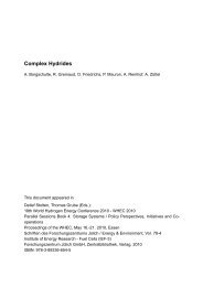
use rather tight bounds on the accuracy of the simulation itself. As an example, figure 2.1
on the next page shows the parameter sensitivities simulated over time, calculated using
both methods, for a Monod-type model with substrate and product inhibitions in a
batch experiment and the maximal specific growth rate as the investigated parameter.
The results of the two methods differed less than 0.1% for all values.
One drawback of the finite differentiation method is the intensive calculation time for
multiple simulations. Even if the parameters are directly changed with an appropriate
amount for all state variables during the whole simulation, the models need to be resimulated
twice for each parameter value. This method was used in the current work
on several occasions for calculation of the covariance matrix of the estimated parameter
values, which has to be done only once for each model. For the design of experiments,
this was not the method of choice, since the parameter sensitivities need to be recalculated
very many times during the optimization process. As an example let us regard
a relatively simple model with 9 parameters and 3 state variables as mentioned in the
simulative study in paragraph 4.2 on page 63. The calculation of all parameter sensitivities
for a simulated batch experiment with 36 measured values in 20 hours, the finite
differentiation method took 2.2 seconds using 98 simulations, whereas the other method
took 0.30 seconds on a personal computer with a pentiumIII 700 MHz processor. One
simulation of the model used in the method of finite differentiation takes much less time
(about 0.022 s) than for the other method, because the simulation of all parameter sensitivities
in the other method makes the model much larger. The effect of the larger
amount of simulations needed for the method of finite differentiation is, however, much
stronger.
24

dy/dµ max
1000
0
−1000
−2000
−3000
0 5 10 15 20
time [h]
2.5. Experimental Design
Figure 2.1.: Jacobian calculated in two ways. Parameter sensitivities are shown for
the concentrations of biomass [OD600h], substrate [gh/L] and product [mMh] depending
on the maximal specific growth rate (µmax). Lines are calculated using explicit simulation
of the sensitivities in the model and the markers by re-simulation with changed
parameter values. Solid lines and × show the sensitivities of the simulated biomass concentrations,
dotted lines and ∗ of substrate concentrations and dashed lines and + of
product concentrations.
2.5. Experimental Design
Every experiment takes time, money and other resources. Therefore it is very important
to limit the number of experiments and get much relevant information from each
experiment. Experimental design stands for techniques which help to plan informative
experiments. Many different approaches have been developed, depending for instance
on the type of information needed and the kind of information available.
The experimental designs can first be divided in two groups which will be called
’statistical experimental design’ and ’model based experimental design’ here. The term
’model based experimental designs’ is used here for designs which use predictions of a
mathematical model in order to determine how an experiment should be performed,
whereas with ’statistical experimental designs’, techniques are meant, which do not
explicitly need these model predictions.
In the current work, model based designs are investigated and used and some of this
type of designs will be discussed in more detail in the following paragraphs.
Examples of statistical experimental designs are for example factorial designs such
as 2-level full factorial designs, where two values are chosen for each variable and all
combinations of these variable values are used. Many different statistical designs have
been used, depending for instance on the type of effects, influential factors and combi-
25

2. Theory
nations, the researcher is looking for. An overview of different statistical experimental
designs can be found in textbooks such as Bandemer and Bellmann (1994) or the review
by Draper and Pukelsheim (1996).
Two different types of model based experimental design techniques are explained and
used here, depending on the goal of the designed experiment. First of all, model discriminating
designs are used for planning of experiments, in order to determine which
of several competing models describe the phenomena best. Second, there are experimental
design criteria, which are used for planning experiments in order to improve the
parameter estimation 11 .
2.5.1. Experimental Design for Model Discrimination
The development of design criteria for discriminating between rival models already dates
back to the sixties, when, amongst others, Hunter and Reiner suggested a criterion
which consists of maximizing the difference between expected measurements y1 and y2,
according to two competing models (Hunter and Reiner, 1965):
ξ ∗ =argmax
ξ (ˆy1 − ˆy2) 2
(2.51)
where ξ describes an experiment and the asterisk denotes the optimized values.
For more than two rival models, either a summation over the model pairs
or a maximization of the minimal distance between two models were suggested
(Cooney and McDonald, 1995; Espie and Macchietto, 1989).
These approaches did not yet take into account the accuracy of the measurements.
However, an expected difference between two accurately measurable values is of course
more informative than the same difference between inaccurate values, so it was suggested
to weight the differences by the estimated variances in the measurements. Especially
when a number of different state variables are measured and also for experiments with
large differences between the measured values, as is usually the case for dynamic experiments,
this is very important since the accuracy of the different measured variables
can differ strongly. For the multivariable and dynamic experiments, also the summation
over all expected measured values has to be introduced:
arg max
ξ
N�
m�
m−1 �
((ˆyi,k − ˆyj,k)σ
k=1 i=1 j=i+1
−2
k (ˆyi,k − ˆyj,k)) (2.52)
where N is the total amount of measurements, including all state variables and all measurement
times. ˆyi,k is the expected measured value k according to model i. σk is the
11 This is also sometimes called ’optimal experimental designs’, but this term has been used in different
ways and can be confusing. Model discriminating designs or statistical designs are also ’optimal’
in a sense and therefore the description ’designs for parameter estimation’ or ’parameter estimation
design’ will be used here.
26

2.5. Experimental Design
expected variance of the difference between the model expectations for measurement k,
which is calculated as the sum of the measurement variances of these expected measurements
for model i and j (Taylor, 1982).
In matrix notation this can be written as:
m−1 �
arg max
ξ
i=1 j=i+1
m�
([ˆyi − ˆyj] T Σ −1
ij [ˆyi − ˆyj]) (2.53)
where yi is a [N ×1] column vector containing the N expected measured values according
to model i:
⎡
⎢
yi = ⎣
yi,1
.
⎤
⎥
⎦ . (2.54)
Σij is a symmetric quadratic matrix of size [N × N], consisting of the sum of the
measurement (co)variance matrices according to model i, Σi and j, Σj:
with Σi defined as:
⎡
⎢
Σi = ⎢
⎣
yi,N
Σij = Σi + Σj
σ 2 i,1 σi,12 ··· σi,1N
σi,12 σ 2 i,2 ··· σi,2N
.
.
. .. ...
σi,1N σi,2N ... σ 2 i,N
⎤
⎥
⎦
(2.55)
(2.56)
where σ2 i,1 is the measurement variance of measurement 1 as expected by model i and
σi,12 is the measurement covariance of expected value 1 and 2 according to that model.
In the summation in equation 2.52, it is assumed that the measurements are independent,
which means that Σ only contains non-zero values in its diagonal and all
covariances are zero.
For the dynamic case, instead of the summation over all N measured values, also the
integration over the experiment time was suggested. However, since we use a limited
amount of discrete off-line measurements in the current work, the discrete description is
shown here.
Besides the measurement error, it was also argued that the variance in the expected
response should be taken into account. This variance originates from the fact that the
simulated values are based on a model which has inaccurate parameter estimates. With
somewhat different parameter values, which might still allow a proper fit to prior data,
the expected values will change. With the sensitivity of the expected values towards the
parameters in jacobian matrix J of size [N × P ], this model variance W (size [N × N])
can be calculated as:
27

2. Theory
W = J · Covθ · J T
(2.57)
The used jacobian matrix of the expected values can be calculated as explained in
paragraph 2.4.4 on page 21, containing the parameter sensitivities of the expected measured
values in separate rows and the sensitivities towards all parameters in separate
columns. The [P × P ] covariance matrix of the parameters, Covθ, can be calculated
from prior data according to equation 2.32 on page 18. Note that the covariance matrix
of the parameter estimates is calculated using the parameter sensitivities of all prior
measured data, whereas the sensitivities J in equation 2.57 are the sensitivities of the
expected new measurements.
The impact of the use of the model variance can be expected to be much stronger
for dynamic experiments than for static ones. The sensitivity of the expected response
towards the estimated model parameters can get rather strong in these experiments.
Furthermore, the parameter sensitivities can have strongly differing values during the
experiment, due to the fact that the influence of the parameters can propagate over
time. The impact of the model variance will increase, when the parameters are less well
estimable, i.e. when the covariance matrix of the parameter estimates has higher values.
Many different model discriminating design criteria have been suggested in literature,
which all contain structures which are similar to the basic structure of equation 2.52
on page 26 (Burke et al., 1997; Hill, 1978). Many of them also use the model variance.
Many of these approaches use a statistical test in which the expected difference
between the model predictions is compared to the estimated variance of this difference
(Atkinson and Fedorov, 1975; Buzzi-Ferraris et al., 1984; Chen and Asprey, 2003), or
calculation of probability density functions (Box and Hill, 1967; Hsiang and Reilly, 1974;
Reilly, 1970). Some of the suggested criteria were developed for special situations such
as discrimination between nested models (Pukelsheim and Rosenberger, 1993), (nested)
polynomes (Dette and Roder, 1997) or autoregressive models (Uosaki and Hatanaka,
1988). A selection of criteria which might be applied to discrimination of dynamic
nonlinear models will be discussed here in more detail.
Box and Hill
The model discriminating experimental design approach of Box and Hill (1967) has been
widely used with and without several adjustments.
They based their criterion on Shannons information theory (Shannon, 1948) using the
concept of system entropy, which can be defined as:
m�
−
(2.58)
Pi ln Pi
i=1
for m models, with relative probability Pi of model i and a total sum of all probabilities
of 1. These relative probabilities can be addressed as shown in equation 2.37 on page 20.
28

2.5. Experimental Design
This entropy is maximal when all models have an equal probability and decreases when
larger differences between the models are detected. The expected change in this entropy
should thus be maximized and this change R canbeformulatedas
R = � Pi,n−1
�
pi ln
pi
� dyn
Pi,n−1pi
(2.59)
where pi is the probability density function of the expected new measurement yn accordingtomodeli.
Box and Hill have used the maximization of a maximal expected value for R, asthe
criterion for a model discriminating design. They formulated their criterion for the
univariate static case with constant measurement variance σ 2 as:
1
arg max
ξ 2
�
m�
m�
i=1 j=i+1
Pi,n−1Pj,n−1
(σ∗2 i − σ∗2 j )2
(σ2 + σ∗2 i )(σ2 + σ∗2 j ) +[ˆyi − ˆyj] 2 ∗
�
1
σ2 + σ∗2 1
+
i σ2 + σ∗2 ��
j
(2.60)
The peculiar use of the upper bound on the expected value for R has been criticized
by several statisticians (Meeter et al., 1970). Reilly suggested a method to estimate the
expected value for R instead (Reilly, 1970).
The use of this maximal value is also the cause for the use of the differences in expected
model variances in the numerator of the first part of the criterion. Especially in dynamic
experiments and in models with poor parameter estimates, the model variances can take
extreme values which can change very fast. This happens, for instance, in situations of
sudden changes such as a depletion of substrate. Therefore it is very likely that, in these
cases, the differences in the expected measured values play no significant role any more,
but the criterion reduces to the maximization of the differences in the model variances,
which is intuitively strange. Several examples where basically only the differences in
the model variances determine the criterion, were also found in the simulative study in
chapter 4.
The calculation of the model variances with the requirement that the model
can be approximated by a linearized form, provides another source of problems
(Bajramovic and Reilly, 1977). Hsiang and Reilly have suggested a method to avoid
this, however requiring the use of a series of discrete parameter sets (Hsiang and Reilly,
1971).
The original criterion from Box and Hill was formulated for one variable and a constant
measurement variance. One option to enhance this criterion for several measured
variables and several measurements in the dynamic experiments, is the summation over
all measured values, assuming all measurements to be independent:
29

2. Theory
arg max
ξ
�
m�
m�
N�
i=1 j=i+1 k=1
(σ 2 i,k
(σ∗2 i,k − σ∗2
j,k )2
+ σ∗2
i,k )(σ2 j,k
Pi,n−1Pj,n−1
+ σ∗2
j,k ) +[ˆyi,k − ˆyj,k] 2 ∗
�
σ 2 i,k
1
+ σ∗2
i,k
+
σ 2 j,k
1
+ σ∗2
j,k
��
(2.61)
where Pi,n−1 still is the probability of model i before experiment ξ, σ2 i,k is the estimated
variance of the expected measurement k according to model i, which might be different
from the corresponding variance of the measurement according to model j: σ2 j,k . σ∗2
i,k
is the model variance of the expected value of measurement k according to model i
(Pritchar and Bacon, 1974).
One problem, which was encountered in the use of the criterion of Box and Hill for
the dynamic bioprocesses in the current project, was an extreme exaggeration of the
differences in the relative model probabilities. This seems to be caused by sensitivity
towards outliers. The exaggeration especially occurred with increasing amounts of measured
values and a clear lack of fit in all models, which is not an unusual situation in
macroscopic modeling of bioprocesses. An alternative option is the calculation of relative
goodness of fit as stated in equation 2.35 on page 20 instead of the relative probability,
which tends to result in much more moderate differences.
Despite the mentioned problems and criticism, the criterion by Box and Hill has been
used successfully in several cases, for instance in heterogeneous catalysis (Froment, 1975;
Froment and Mezaki, 1970) or in continuous fermentations (Takors et al., 1997).
Buzzi-Ferraris and Forzatti
Buzzi-Ferraris and Forzatti (1983); Buzzi-Ferraris et al. (1990, 1984) suggested an intuitively
appealing discriminating design criterion which is based on the statistical chance
that a difference between two model predictions could also be explained by the variance
of the predictions (both by measurement inaccuracy and inaccurate parameter
estimates). They suggested maximizing the ratio between the expected differences in
the model predictions and the total variance of this difference, which was build up from
the measurement variance and the model variances.
m−1 �
arg max
ξ
i=1 j=i+1
m�
[ˆyi − ˆyj] T V −1
ij × ([ˆyi − ˆyj]+trace[2ΣV −1
ij ]) (2.62)
where the variance matrix Vij consists of two times the measurement variance matrix
Σ and the model variances of model i and j:
30
Vij =2Σ + Wi + Wj
(2.63)

2.5. Experimental Design
The model variances W are also explained in equation 2.57 on page 28.
Buzzi-Ferraris and Forzatti published their criterion with a model independent variance
matrix Σ. In the current work, the terms 2Σ in equation 2.62 and 2.63 have been
replaced with Σi + Σj, the sum of the estimated measurement variances of the expected
values according to model i and j, which allows a different measurement variance at
different values.
Buzzi-Ferraris and Forzatti suggested the addition over all model pairs as shown in
equation 2.62 and did not use of the weights of the importance of the model pairs as
done for instance by Box and Hill. Instead, they stated that all models which passed
the chi-squared adequacy test based on all prior data, should be regarded with equal
probability and all other models should simply not be regarded. When models which
did not pass the test before, pass the test after addition of new data, the model could
be reintroduced for the construction of the next experiment.
Buzzi-Ferraris and Forzatti also suggested to stop the procedure when it would fail to
design experiments which give higher values for the criterion than the amount of new
expected measurements, claiming that the experiment is not expected to be informative.
Such a criterion seems appealing, but is somewhat problematic in the suggested form
for the use in multiresponse experiments since it actually suggests that the average of
the expected responses should be informative. It could however very well be, that many
measurements and many variables are not informative, having practically equal responses
according to both models, whereas only a few expected measurements are expected to
differ significantly. In this case the experiment would be rejected, although the same
experiment would be accepted when only these relevant measurements would be planned.
One other option could therefore be to accept only experiments which expect at least
one measurement to be informative.
Chen and Asprey
Based on the criterion by Buzzi-Ferraris and Forzatti, Chen and Asprey recently published
a similar criterion for dynamic experiments and multiresponse nonlinear situations
with discrete sampling (Chen and Asprey, 2003):
arg max
ξ
nsp �
i=1
[ˆyi − ˆyj] T S −1
ij [ˆyi − ˆyj] (2.64)
using an addition over all suggested sampling points nsp. So, all sampling points are
regarded independent, also with respect to the model variance which is caused by the
parameter estimates, which seems strange. The [nv×1] vectors of expected measurements
y contain the nv different measured variables at one sampling time, and all these variables
were suggested to be dependent. Also the [nv × nv] matrix with variances, Sij, contains
the covariances at one sample time only. Note that this criterion is equal to a criterion
31

2. Theory
with all measured values in one vector and a corresponding bigger covariance matrix,
when all covariances between two measured values which are taken at different sampling
times, are zero.
The weighting by Vij has been replaced by the very similar Sij, which however contains
the measurement variance only once:
Sij = Σ + Wi + Wj
(2.65)
They suggested to estimate the experimental variance from prior data and did not include
the possibility of having different expected measurement variances based on different
model predictions.
Furthermore, they used their criterion only for one model pair at a time and suggested
to use it on the two best fitting models in one of their examples.
Based on the suggestion of Buzzi-Ferraris and Forzatti, also Chen and Asprey suggested
not to perform any experiments which give rise to criteria smaller than the amount
of measurements, being all measured variables at all sampling times together. This has
been discussed above for the criterion of Buzzi-Ferraris and Forzatti. An example of an
experiment which would not pass this criterion, but which would be accepted when only
some of the measurements are taken, is shown in the simulative study in chapter 4.
The criterion by Chen and Asprey has been used in a simulative comparison in the
current work with the adjustment that the criterion was added over all model pairs, just
like suggested by Buzzi-Ferraris and Forzatti, and with the measurement variance of the
expected measurements being the average between the ones estimated for the 2 models.
Discriminating Design Criteria for Dynamic Experiments Without Model Variances
The calculation of model variances and the parameter sensitivities which are needed
for this, is a rather difficult task for dynamic experiments, as is also pointed out in
paragraph 2.4.4 on page 21. Furthermore, the model variances can take extreme values
when used in dynamic systems and with models with poor parameter estimates. Besides
the problems this may cause in the calculation of the experimental designs, also the
fact that a large part of the calculation time is used for the calculation of the model
variances, is an important disadvantage of these design criteria. For example, calculation
of the criterion of equation 2.51, which does not use the model variance, for a simple
Monod-type model with 3 measured variables and 9 model parameters and a simple
batch experiment of 20 hours duration with 12 samples, took approximately 0.08 s.
Calculation of the criteria with model variances, such as equation 2.61 and 2.62, on
the other hand, took about 0.8 s in the same situation on a personal computer with a
PentiumIII 700MHz processor!
In this respect, it should also be mentioned that it can already be difficult and timeconsuming
to include all derivatives of the differential equations towards the parameters
and the state variables in the models, which is needed for calculation of the model
32

2.5. Experimental Design
variance. This is especially so when the models get more complex. In a more automated
model building, this might however be done automatically using symbolic mathematical
tools.
Clear examples of criteria which do not use a model variance are the criterion by
Hunter and Reiner (equation 2.51) or the similar criterion with weighting by the measurement
variances (equation 2.53).
Based on these criteria, some extensions are presented here, in an attempt to improve
the criteria for the use in dynamic multivariable experiments.
The first extension is introduced to consider the variance in the timing of the sampling,
which can highly influence the measured values. Regard, for instance, the expected
measured values of one variable according to two competing models, shown in figure
2.2. The values change very fast in the final part of the curves, but not exactly at
the same time. This temporarily causes relatively large differences, especially when
compared to the low values of the expected measurements themselves, although the
curves stay close to each other. This is a situation which can easily occur when using
y
25
20
15
10
5
0
0 5 10
time [h]
15 20
Figure 2.2.: Expected responses of two competing models (one shown as a solid line
with + and one dashed with ×) for a designed dynamic experiment. Due to the fast
changes in the measured values in the final part of the experiment, the differences between
the models are relatively high, also when the curves are close to each other.
criteria like 2.53 to design dynamic experiments. However, such situations are not likely
to be very informative for discrimination between the two models. In many cases, the
model variances get relatively high in these situations. Therefore, such less informative
situations can be avoided by criteria which are weighted by the model variance, such as
the criteria by Buzzi-Ferraris and Forzatti or Chen and Asprey, shown in the preceding
two paragraphs. One other way to account for this problem is by introducing a part
of the measurement variance which is based on the variances in the measurement time,
33

2. Theory
which can be estimated using:
dyi
σi,t = st
dt
(2.66)
where σi,t is the standard deviation of the expected measurements yi, according to
model i, caused by the variance in the measurement time point which is described
using a standard deviation st and the time derivative of the estimated response dyt
dt .
This time derivative is already needed for the simulations of the models and is therefore
available without much extra computational effort. The standard deviation of the timing
is dependent on the way of sampling and handling of the samples and can be estimated
from timing of a series of measurements in practice. In the current work, a standard
deviation of 10 minutes was used.
When all measured values are assumed to be independent, the corresponding squared
values of equation 2.66 can be used in the diagonal of a larger timing dependent covariance
matrix of all measurements. However, when a sample is taken somewhat delayed,
this will count for all state variables measured in this sample, so this part of the measurement
error is assumed to be correlated amongst measured values taken from the
same sample, but not between values from different samples. For one sample with all
measured values in an [nv × 1] column vector yi(s) and the corresponding timing dependent
part of the standard deviation σi,t(s) in a column vector of the same size, the
[nv × nv] covariance matrix Σi,t(s) caused by the timing error could be calculated as:
Σi,t(s) =σi,t(s) · σi,t(s) T
(2.67)
For experiments with more than one sample, the covariance matrices for each sample
can be used as parts of the total timing dependent covariance matrix with the covariances
between measured values from different samples being 0, assuming no correlation
between the errors in the timing of the different samples. So, when we use the column
vector of all N = nv · ns expected measurements with first all nv measured variables
from the first sample yi(1), then all from the second sample yi(2), etc:
⎡ ⎤
yi =
⎢
⎣
yi(1)
.
yi(ns)
⎥
⎦ (2.68)
we can use the covariance matrix of the measurement error caused by the timing errors
as:
⎡
[Σi,t(1)]
⎢
Σi,t = ⎢ 0
⎢
⎣ .
0
[Σi,t(2)]
0
...
0
. ..
0
.
0
⎤
⎥
⎦
(2.69)
0 ··· 0 [Σi,t(ns)]
34

2.5. Experimental Design
The squared brackets are added around the timing dependent covariance matrix of the
values from the first sample Σi,t(1) to the last of ns samples Σi,t(ns), to emphasize the
fact that these are [nv × nv] matrices taken from equation 2.67 and not just scalars.
Now, this matrix can simply be added to the corresponding covariance matrix Σi,m,
caused by measurement errors such as dilution inaccuracy or the accuracy of the used
analytic equipment
(2.70)
Σi = Σi,m + Σi,t
and used in the criterion formulated in equation 2.53 and 2.55.
Obviously, when the measurement variance would be determined from replication of
complete experiments, this part of the measurement error, caused by timing of the
sampling, would be included in the measurement variance. This would, however, not
be the case when the measurement variance would be determined solely based on the
accuracy of the analytical methods or repeated measurement from one sample.
Another adaptation of the simple criterion of 2.53 on page 27 comes from the idea
that, in dynamic experiments, besides the difference between the expected values, also
the difference between the expected shapes of the curves is likely to improve the discrimination
between models. To elucidate this idea, regard the curves in figure 2.3. The
fact that the two curves have clearly different shapes is expected to provide a better
discrimination than when both curves would stay horizontal, although this would result
in the same distance between measured points.
y
35
30
25
20
15
10
5
0
0 5 10 15 20
time[h]
Figure 2.3.: Expected responses of two competing models (one with a solid line and
+ and the other as dashed line with ×) for a designed dynamic experiment. It is
hypothesized that the different shapes of the two curves around 10 hours makes a good
discrimination more likely than when both curves would have stayed on a constant
distance.
35

2. Theory
One option to account for this, which is suggested and tested here, is by regarding the
changes in the expected values between subsequent discrete measurements by extending
the design criterion to:
m−1 �
arg max
ξ
i=1 j=i+1
m�
([ˆyi − ˆyj] T Σ −1
ij [ˆyi − ˆyj]) + ([ ∆y ˆ
i − ∆y ˆ
j] T Σ −1
∆ij [ ∆y ˆ
i − ∆y ˆ
j]) (2.71)
where ∆ˆy i is a column vector of length (N − nv) containing the differences between all
subsequent expected measurements according to model i:
⎡
∆y ˆ ⎢
i = ⎣
ˆyi(2) − ˆyi(1)
.
ˆyi(ns) − ˆyi(ns − 1)
⎤
⎥
⎦ (2.72)
and Σ∆ij is a square [N − nv × N − nv] covariance matrix which is used to weight this
added part of the criterion, which can be calculated as:
Σ∆ij = Σij(1 : ns − 1) + Σij(2 : ns) (2.73)
where Σij(1 : ns − 1) denotes the covariance matrix containing measurement errors and
timing errors, as mentioned before, but using only samples 1 to ns−1, so disregarding the
final sample. Analogous, the first sample is omitted in Σij(2 : ns). This way, the squared
difference ˆyi(2)− ˆyi(1) is weighted by the expected variance of this difference, consisting
of the addition of the variances of both subsequent measurements. The covariance
matrices Σij(1 : ns − 1) and Σij(2 : ns) can be estimated as the covariance matrix
due to real measurement errors and due to the variance in sampling times as mentioned
above.
2.5.2. Experimental Design for Parameter Estimation
As mentioned in paragraph 2.4.2 on page 18, the accuracy of the parameter estimation
depends on the quality of the data. Experimental design techniques for parameter
estimation aim at designing experiments in order to get good quality of the data for
parameter estimation.
Also the covariance matrix of the estimated parameter as a measure for the accuracy
of the parameter estimation was already introduced in paragraph 2.4.2. A parameter
estimating design will try to minimize the expected values in this covariance matrix.
It is common practice to work with the inverse of the covariance matrix of the parameter
estimates: the informationmatrix M 12 :
M = Cov −1
θ = JT · Cov −1
m · J (2.74)
12 Analogue to the Fisher informationmatrix. This matrix originates from the communication theory of
36
Shannon (Shannon, 1948).

2.5. Experimental Design
For the current theoretical explanations, it may be more convenient to work with the
covariance matrix. In practice, however, one might want to avoid the need for calculation
of the inverse of a matrix.
The determinant of M is always zero or positive. If the determinant of M is zero,
not all parameters can be estimated. This happens, for instance, when the amount of
measurements is less then the amount of parameters. This would lead to a jacobian J
with a lower rank than the amount of parameters. Another characteristic of M, which
is mentioned here because it may be helpful in understanding the algorithms, is the
additive character:
M(ξ1+2) =M(ξ1)+M(ξ2) (2.75)
assuming both experiments to be independent, with ξ indicating an experiment, M(ξ1),
the information matrix according to experiment 1, M(ξ2), the information matrix according
to experiment 2 and M(ξ1+2), the information matrix when the measurements
of both experiments are regarded together (still being independent from each other).
More detailed mathematical information on the information matrix or the covariance
matrix can also be found in textbooks such as Bandemer and Bellmann (1994).
In order to understand the experimental design criteria for parameter estimation, it
can be very helpful to try to visualize the meaning of the covariance matrix of the
parameters.
Assuming normally distributed measurement errors, the probability density function
for a set of parameters θ close to the estimated parameters ˆ θ canbeformulatedas
p(θ) =(2π) −r/2 (det Covˆ θ ) −1/2 �
exp − 1
2 (ˆ θ − θ) T Cov −1
ˆθ (ˆ �
θ − θ) . (2.76)
with r being the number of parameters. This probability density function is constant
when
( ˆ θ − θ) T Cov −1
ˆθ (ˆ θ − θ) =constant (2.77)
This function 2.77 describes the surface of an r-dimensional ellipsoid with the parameter
sets inside this ellipsoid all having a higher probability than the sets outside. For the
simple case with only two parameters (r = 2), the ellipsoid becomes an ellipse which can
easily be visualized as in figure 2.4.
The more accurate the parameter estimates are, the smaller this ellipsoid will be. Several
criteria have been suggested which aim at minimizing different aspects of the size of
the ellipsoid of which some will be mentioned here. More details can also be found
in reviews and textbooks such as Atkinson (1982); Bandemer and Bellmann (1994);
Walter and Pronzato (1990).
An often used criterion for parameter estimating experimental designs is to aim at the
minimization of the expected volume inside the ellipsoid. Except for a constant factor,
this volume equals � det Covˆ θ . Experimental designs which aim at minimizing this are
37

2. Theory
θ 2
$θ 2
0
area ≅ det( Cov $θ )
Figure 2.4.: Confidence ellipse of the parameter estimates for 2 parameters. The area
inside the ellipse corresponds to the square root of the covariance matrix of the parameter
estimates, which is used in a D-optimal design.
called D-optimal designs:
ξ ∗ =argmin(det(Covˆ
ξ
θ )) = arg min(
ξ
$θ 1
θ 1
1
) (2.78)
det(Mˆ θ )
Besides this D-optimal design criterion, several other criteria have been suggested
based on the covariance matrix of the parameters. A design is called A-optimal when
the trace of the covariance matrix is minimized, which corresponds to the minimization
of the average length of the axes of the ellipsoid:
arg min(trace(Covˆ
ξ
θ )) = arg min(trace(M
ξ −1
ˆθ
)) (2.79)
The E-optimal design on the other hand aims at the minimization of the largest
axis of the ellipsoid by minimization of the largest eigenvalue of the covariance matrix
λmax(Covˆ θ ):
arg min(λmax(Covˆ
ξ
θ )) = arg min(λmax(M
ξ −1
ˆθ
)) (2.80)
Munack (1989) suggested to minimize the ratio between the longest and the shortest
axis of the ellipsoid: the modified E-criterion or the Λ optimality criterion:
arg min
ξ ( λmax(Covˆ θ )
λmin(Covˆ θ ) )=argmin
ξ
−1
ˆθ
(λmax(M )
λmin(M −1
ˆθ
) ) (2.81)
This criterion was introduced, because an ellipsoid which is long in one direction means a
set of parameter is not uniquely estimable, since a linear combination of the parameters
will be accepted. Baltes et al. (1994) extended the Λ optimality criterion in an attempt
to avoid extreme fast changing experimental conditions, which would deteriorate the
38

2.5. Experimental Design
validity of the unstructured kinetic models. Berkholz wanted to avoid experiments which
performed very poor as a production experiment and extended the Λ optimality criterion
accordingly (Berkholz et al., 2000). The fact that the modified E-criterion regards the
shape of the ellipsoid rather than the volume, can result in larger confidence intervals
of the parameter estimates after the designed experiment than, for instance, using the
D-optimal or E-optimal designs (Faller et al., 2003).
When the estimation of just one parameter or a certain set of parameters should be
improved, the C-optimal design can be used, where the vector c is used to select and
possibly weight the parameters.
arg min(c
ξ T (Covˆ θ )c) =argmin(c
ξ T (M −1
ˆθ
)c) (2.82)
Besides the designs which use the covariance of the parameter directly, also design
criteria have been suggested which regard the variance of the expected measured values
of the new experiment (the model-variance, see also paragraph 2.5.1 and equation 2.57
on page 28), such as the G-optimality criterion which aims at minimizing the maximal
expected variance of the expected measurements:
arg min
ξ max(j T (Covˆ θ )j) (2.83)
where j is a column vector of parameter sensitivities of the new measurement.
Lee (1987) suggested to combine several of the mentioned criteria, optimizing one
criterion with the constraint of reaching a minimal quality with respect to another criterion.
For the current work the D-optimality criterion (equation 2.78) was chosen and implemented
in the programs.
2.5.3. Experimental Design for Model Discrimination and Parameter
Estimation
Experiments which are optimal for discrimination between competing models are not
necessarily useful for the improvement of the parameter estimation and vice versa.
To reach the final useful model, both problems, model discrimination and parameter
estimation, need to be solved. Both problems are interconnected: the model discriminating
designs are based on model predictions which can be very inaccurate when the
parameters are poorly estimated, but one model structure needs to be selected for the
use of a parameter estimating design.
One option, which is also suggested in the current work, is to use two separate different
design criteria and design each experiment for either of the two purposes. First a model
needs to be selected using a discriminating design criterion and as soon as one model
is selected, its parameter can be estimated better after following experiments which are
39

2. Theory
designed using a parameter estimation criterion (Chen and Asprey, 2003; Froment, 1975;
Montepiedra and Yeh, 1998).
However, also some suggestions were made to use one criterion for the dual problem
(Fedorov and Khabarov, 1986; Ford et al., 1989; Froment, 1975). Although they will not
be explained in detail here, some are mentioned shortly. For instance, Hill et al. (1968)
used a weighted combination of both criteria. Borth (1975) later published an entropy
criterion adapted from the model discriminating criterion from Box and Hill. Spezzaferri
(1988) used a multiplicative combination of two criteria and Pronzato (2000) suggested
the use of a penalty function for poor parameter estimation in a model discriminating
design criterion.
2.6. Optimization of Bioprocesses
Bioprocesses are optimized at different stages: strain development, development of
the production process and optimization of the industrial plant, which are, however,
closely interconnected (Roubos, 2002). Optimal process conditions, for instance, depend
strongly on the used strain.
Using modern genetic techniques, strain improvement and improvement of process
conditions and the medium are more and more parallel processes. In the current work,
however, the used strain, the type of bioreactor and to a large extent also the used media
are assumed to be selected already. Nevertheless, suggestions for strain improvement
may very well come from identification of limitations during improvement of the process
conditions or the medium using the techniques presented in the current work.
In order to optimize a process, first a performance function is needed. In industrial
processes, this can be a rather complex function depending on many interconnected
steps in the process (Yuan et al., 1997). Optimization of the biological reactions is
usually of high importance. The overall yield of product on substrate, the total volumetric
productivity, the purity of the product or the quality of a complex product
are some of the common criteria to be optimized with respect to the biological process
(Heinzle and Saner, 1991).
Two strategies of process optimization can be distinguished: model based optimization
and empirical optimization. In the latter case, search techniques such as simplex
methods, gradient searches, or genetic algorithms can be used with sequential experiments
in order to improve the process. For instance, WeusterBotz et al. (1997) have
used a genetic algorithm to optimize the trace element composition for cultivation of
a Corynebacterium glutamicum strain. The review by Schügerl (2001) contains other
examples of the use of empirical optimization strategies for optimization of bioprocesses.
For more complex processes with many control parameters, as is usually the case for
optimization of trajectories in fed-batch processes, such search techniques may prove
to get very laborious and converge slowly. When a proper process model is available,
40

2.7. L-valine Production in Corynebacterium glutamicum
the optimal settings of the control parameters can be calculated off-line without further
experiments. In some relatively simple cases, this may be possible analytically. For
more complex systems with many state variables and control parameters, this becomes
complicated or even impossible, so numerical techniques have to be used.
The calculated optimal trajectories can then be applied in the process directly (feedforward
control), as is also done in the example by Lee et al. (1997) and in the current
work in paragraph 5.2.6. Since the process model, the initial conditions and the controlled
variables all include inaccuracies, it is, however much, better to include feedback
control based on online measured values. This measured variable can be simply the
variable which was intended to be controlled, such as the pH or temperature, or an
online measurable substrate concentration. Or, if this variable is not measurable online,
it may be possible to control a derived variable instead. Biomass growth can, for
instance, be monitored by measurement of the oxygen consumption rate and carbon
dioxide production rate (Golobic et al., 2000).
The availability of a model which can be used for model based optimization may also
allow for the use of model based predictive control. Here, the prediction of the model is
calculated regularly online and the optimal control is calculated, using this prediction,
for a limited time. The basic concepts and an overview of model predictive control
can be found in Garcia et al. (1989); Henson (1998). Preuss et al. (2000) applied model
predictive control for the glucose feed for the growth of yeast in a fed-batch culture.
Another example is the optimization of ethanol production by Zymomonas mobilis by
Hodge and Karim (2002).
2.7. L-valine Production in Corynebacterium glutamicum
In the current project, the aim is to produce L-valine using a genetic modified strain of
C. glutamicum.
The gram positive, nonmotile, non spore forming bacterium C. glutamicum is
generally regarded as safe (GRAS). It has already been isolated in 1957 in a screening
for L-glutamate producing bacteria in soil by Kinoshita and co-workers (Kinoshita et al.,
1957) and it is nowadays widely used for the fermentative production of natural amino
acids such as L-glutamic acid and L-lysine(Burkovski, 2003a; Hermann, 2003). Due
to its industrial importance and its GRAS status, it has been investigated very intensively,
which resulted amongst other things in the complete sequencing of its genome
in several strains (Degussa, Kyowa Hakko Kogyo, BASF (Ikeda and Nakagawa, 2003;
Kalinowski et al., 2003)). Besides the investigation of the genome, also the transcriptome
13 (Hayashi et al., 2002; Krömer et al., 2004; Muffler et al., 2002; Wendisch, 2003),
13 The investigation of the transcriptome indicates the investigation of the gene expression.
41

2. Theory
proteome14 (Hermann et al., 2001) and the metabolome15 (Chassagnole et al., 2003;
Drysch et al., 2003; Park et al., 1997; Sahm et al., 2000; Vallino and Stephanopoulos,
1993; Varela et al., 2003; Wittmann and Heinzle, 2001) are thoroughly investigated.
This also resulted in the availability of many tools for genetic modifications of
C. glutamicum (Nampoothiri and Pandey, 1998).
C. glutamicum needs biotin for growth, which was an important characteristic because
the glutamate production was triggered by biotin limitation in wild-type strains
(Shiio et al., 1962). Nowadays, with modern biotechnological techniques, also other
growth limitations and other mechanisms are available to achieve overproduction of
amino acids (Kimura, 2002), as is also the case in the organism which is used in the
current study.
Another characteristic of C. glutamicum, which may be of importance for its use, is the
complex cell envelope containing mycolic acids (Bayan et al., 2003; Christensen et al.,
1999), which are typical for Corynebacteriaceae, Mycobacteriaceae, Nocardiaceae and a
few small other families (Glazer and Nikaido, 1995). These mycolic acids form an extra
hydrophobic barrier which probably causes the low permeability of the cell wall for
hydrophilic compounds (Jarlier and Nikaido, 1990). Hydrophilic compounds therefore
have to pass the cell wall through a channel (Costa-Riu et al., 2003a,b).
CH3 COO
H3C -
L-Valine is a natural proteinogenic amino
acid and it is one of the essential amino acids
for humans. Together with leucine and alanine,
it forms the pyruvate family of amino
acids. Furthermore, it is a branched chain
amino acid just like leucine and isoleucine.
It is a fairly hydrophobic (logp =1.64), neutral
amino acid (pI=5.96), which makes it
NH +
3
likely that it may be able to pass the cell
membranes relatively good through passive
diffusion (Krämer, 1994). The structure of
Figure 2.5.: L-Valine
L-valine is shown in figure 2.5.
The annual production of L-valine is
about 1000 tons, which is among the smaller amounts for natural proteinogenic amino
acids (Drauz et al., 2003; Eggeling et al., 2001; Leyval et al., 2003). It is mainly being
used in infusion fluids and special dietary nutrition. However, also beneficial effects
of addition of L-valine to pig- and chicken feed were reported (Boyd et al., 2000;
Harms and Russell, 2001; Kidd et al., 2000).
L-Valine is currently being produced by isolation from protein hydrolysates,
in fermentative processes or by enzymatic resolution of N-acetyl-D,L-valine
14 The proteome indicates the proteins which are present in the cells.
15 The intracellular concentration of metabolites: intermediates and products of metabolic pathways.
42

2.7. L-valine Production in Corynebacterium glutamicum
(Bodalo-Santoyo et al., 1999). The fermentative production of L-valine is performed using
either α-aminobutyric acid-resistant mutants of Serratia marcescens or coryneform
bacteria such as Corynebacterium or Brevibacterium (Drauz et al., 2003). Brevibacterium
strains are actually nowadays regarded as a subspecies of Corynebacterium, since
both organisms could not be distinguished at the rRNA level (Liebl et al., 1991). Besides
these two groups of bacteria, also several other L-valine accumulating micro-organisms
have been reported (Chatterjee and Chatterjee, 1982; Chattopadhyay and Banerjee,
1978; Mandal and Majumdar, 1973). The fermentative production of up to 10 g/L
L-valine by C. glutamicum was already published in the sixties (Nakayama et al., 1961)
and already in 1977, almost 40 g/L was reported, produced by a Brevibacterium lactofermentum
using limited oxygen supply (Akashi et al., 1977). Brevibacterium lactofermentum
AJ12341 is reported to produce 39 g/L L-valine at 28 % yield (Drauz et al., 2003).
Although the total yearly production volume is not very large, it is expected to
grow steadily (Hermann, 2003) and there is a strong interest in further improvement
of the fermentative production processes, as is also illustrated by the European research
project VALPAN: ’construction of C. glutamicum strains producing either L-valine or
D-pantothenic acid - a rational approach using genome research’, which took place from
February 2001 until March 2004 (Puhler and Tauch, 2003). The strain which is used in
the current work, was also used in the VALPAN project.
In the natural production of L-valine, two molecules of pyruvate are used to produce
one molecule L-valine. This metabolic pathway is described in more detail in paragraph
5.1.1 on page 87, where also the genetic modifications of the used strain are
mentioned.
43

2. Theory
44

3. Dynamic Modeling Framework
In this chapter, some remarks are made on the developed and used programs for modeling
of dynamic processes using special experimental design techniques. The programming
was done in Matlab, using Simulink for dynamic simulations. Most programs were
written as functions. Their use and the ideas behind them are explained here and in
more detail in the documentation in the program code.
3.1. The Modeling Procedure
A schematic flowsheet of the suggested modeling procedure with experimental designs
is shown in figure 3.1.
Since we need the parameter estimates and their accuracies in order to use the experimental
design techniques, the first data are taken from intuitively planned preliminary
experiments. A first set of simple models is based on these data and available information
on the biological system and the model parameters of these models are estimated
by fitting the models to the data from these intuitively planned experiments. Enough
data have to be gathered and the used models have to be relatively simple, so all model
parameters can be estimated.
After this initialization, the model based approach is started. First, an iterative
approach for model discrimination using experimental designs is performed, resulting in
one selected model. The parameters of this selected model may still be partly poorly
estimable from the available data. In a subsequent iterative process, the parameter
estimation can then be improved, using special experimental designs for this purpose.
The resulting model can be used for optimization and control of the final process.
The different steps in the modeling procedure are explained in more detail in the
following paragraphs.
45

3. Dynamic Modeling Framework
iterative model discrimination
iterative parameter estimation
start model development
preliminary experiments
setup first model structures
parameter regression
compare model fits
experimental design for model discrimination
experiment i
parameter regression
some models fit?
compare model fits
model identified?
Yes
experimental design for parameter estimation
experiment j
parameter regression
selected model
parameter known
exact enough?
model
Yes
Yes
No
No
i=i+1
adjust model structures
Figure 3.1.: Schematic flowsheet of the modeling procedure using experimental design
techniques.
46
No
j=j+1

3.2. Parameter Estimation
3.2. Parameter Estimation
After each experiment, be it intuitively planned or designed for model discrimination or
parameter estimation, the parameters of the models are re-estimated using all available
(prior and new) data.
It turned out to be very important to limit the allowed parameter space as much as
possible, especially when the models are large and nonlinear. Many of the parameters
in the kinetic models are directly correlated to characteristic values which are calculable
from measured values, such as the yields and the specific rates of growth, consumption
and production. With the calculated values from available measured data, tight bounds
on parameters can be set.
Within this limited parameter space, the parameters are estimated by a non-linear
least squares technique using the maximum likelihood criterion explained in paragraph
2.4.1 on page 17.
The standard deviation of the measurements are calculated in the same way as suggested
by Wiechert (Takors et al., 1997; Wiechert, 1990):
�
σy = y · σy,rel,min · 1+
1
( y
lby )2 + y
lby
�
(3.1)
using a constant minimal relative error of σy,rel,min and an increasing relative error
at decreasing measured values y due to the introduced lower accuracy bound on the
measurement, lby.
First a global minimization within the allowed parameter space is performed using
a genetic algorithm 1 . The resulting set of parameters is then optimized further locally
using a bounded nonlinear least squares routine 2 .
The used genetic algorithm also allows (but does not necessarily need) the suggestion of
parameter values by the user, which may save a lot of calculation time before reaching
convergence. The user supplied suggestion can for instance be the set of parameter
values which was estimated before, based on prior data in the prior iterative loop. The
differential evolution program which is used for optimization of design parameters (see
paragraphs 3.3.1 and 3.3.2 on page 49) does not foresee this user supplied initial guess and
is therefore not used here. With slight adjustments, the parameter estimation program
has also been used without the global search or with re-estimation of only a selection of
the parameters.
1 The used freeware Matlab algorithm is implemented by and available from MathWorks
(www.mathworks.com) and based on the algorithm described by Goldberg (1989).
2 The function lsqnonlin, taken from the Matlab optimization toolbox, uses an algorithm which is based
on Coleman and Li (1996).
47

3. Dynamic Modeling Framework
3.3. Designing Experiments
3.3.1. Model Discriminating Design
Five model discriminating design criteria, adjusted for the dynamic multivariable experiments,
were implemented in the Matlab programs. See also paragraph 2.5.1 on page 26
for more information on the used criteria. The criterion by Box and Hill (equation 2.61
on page 30) was implemented using a summation over all measured variables and all time
points, assuming all measurements to be independent. The criterion by Buzzi-Ferraris
and Forzatti (equation 2.62) was used with the matrix of model variances including
covariances, but independent measurements with respect to the measurement variance
matrix, which therefore contained non-zero values only in its diagonal. The criterion by
Chen and Asprey (equation 2.64 on page 31) was adapted for the use with more than
two models by a summation over all model pairs, although it was originally used only
for the two closest competitors among the models. Besides these three design criteria
which use the model variance, two criteria were implemented without this variance of
the model prediction. First the criterion by Hunter and Reiner, weightedbythe
expected measurement variances (equation 2.53 on page 27) was implemented, assuming
all measurements to be independent. Finally, also a similar criterion was used, but with
the use of a time dependent measurement variance and including an extension regarding
the shape of the curve, as shown in equation 2.71 on page 36.
These five criteria were all used in a simulative study, as mentioned in chapter 4 on
page 61, and two of them have been applied during the process development of the
L-valine production process. The first model discriminating design during this process
development (paragraph 5.2.3 on page 104) was realized using the adjusted Box and Hill
criterion and the second model discriminating design (paragraph 5.2.5 on page 113) was
proposed using the criterion without the model variance with the extensions mentioned
above.
The design parameters for a new experiment (see paragraph 3.4.1 on page 50) are
first searched for in a bounded parameter space using the global optimization algorithm
’differential evolution’ 3 , which is thought to be more efficient than the genetic algorithm
used for parameter estimation. After the global search, the parameters are further
optimized locally using a simplex algorithm 4 , starting from the results of the global
optimization. Since the used simplex algorithm works in an unlimited parameter space,
the parameters are converted from the limited to the unlimited space by
� �
θlim − lbθ
θunlim =0.5ln
ubθ − θlim
(3.2)
3
This freeware function was programmed by Rainer Storn and more information is available at
www.icsi.berkeley.edu/ storn/code.html.
4
The function ’fminsearch’ from the Matlab optimization toolbox was used
48

and back by
�
θlim = lbθ +(ubθ − lbθ)
e θunlim
e θunlim + e −θunlim
3.3. Designing Experiments
�
, (3.3)
where the real parameter θlim, being limited between lower bound lbθ and upper bound
ubθ, is projected to the unlimited parameter value θunlim.
The fitted models are evaluated by visually judging the plots of the concentrations over
time and the scaled residuals (the difference between measured- and simulated values,
weighted by the standard deviation of the measured values) over time. Furthermore,
the models are evaluated by calculating reduced chi squared values, as described in
paragraph 2.4.3 on page 19.
Especially during the initial phase of the model development, the available data might
not be enough to describe all important features of the process properly, resulting in
oversimplified models. Therefore, it is not unlikely that none of these models fit satisfactory
after a new designed experiment. In such a case, the model structures need to
be adjusted.
The model discrimination procedure is iterative. If several of the resulting models fit
satisfactory, a new model discriminating experiment can be designed. When only one
model is accepted, or when the remaining models do not predict significantly different
results in the relevant range, the model discrimination is stopped. If needed, additional
experiments can then be planned in order to improve the parameter estimates of the
selected model.
3.3.2. Design for Parameter Estimation
The implemented design criterion for designing experiments to improve the estimation of
the model parameters, is the D-optimality criterion, which is explained in paragraph 2.5.2
on page 36.
The optimization of the design parameters for the new experiment (see paragraph
3.4.1) is performed similar to the model discriminating design as described in the previous
paragraph. First a global optimization is performed in a bounded parameter space
using the differential evolution algorithm, followed by local optimization using a simplex
algorithm starting from the values supplied by the global search.
Also the parameter estimating experimental design strategy is iterative. After each
experiment, the model parameters are re-estimated and the parameter estimation is
evaluated. This evaluation is done by calculating the covariance matrix of the parameter
as described in paragraph 2.4.2 on page 18. The square root of the diagonal of this
covariance matrix, e.g. the standard deviations of the parameter estimates, is compared
to the estimated parameter values. Furthermore, a correlation matrix is calculated from
the covariance matrix according to equation 2.33 on page 19, in order to see whether the
model parameters are strongly correlated.
49

3. Dynamic Modeling Framework
3.3.3. Design an Optimized Production Process
The offline calculation of an optimized production process can be performed very similar
to the calculation of experiments which are optimized for model discrimination or
parameter estimation, instead of production.
In the current work, the total volumetric productivity was used as a criterion to
be maximized in the optimal production process. This criterion is also mentioned in
paragraph 3.4.3 on page 59.
Again, a local optimization by a simplex algorithm is performed, starting from the
results of a bounded global search using the differential evolution algorithm.
3.4. Application: L-Valine Production Process Development
Several details of the presented modeling procedure are specific for the modeled process
and the constraints on the system. In the current section, some remarks are made
considering the application of the experimental design techniques for modeling and optimization
of the L-valine production by C. glutamicum. First of all, the description of
the designed experiments and its constraints are listed. Furthermore, some remarks are
made on the use of the actual measured data in the modeling procedure.
3.4.1. Designed Experiments
A designed fed-batch experiment will normally consist of parameters which describe the
initial conditions and the time-variant feedrates. Furthermore, user-supplied limits on
the parameter values and constraints on the course of the fermentation can be involved.
For very small scale or with special equipment where the number of samples which can
be taken is limited, also the measurement time points may be optimized.
For modeling of the L-valine production process, the experiments were planned using
the following constraints:
50
• The maximal fermentation time was fixed to 48 hours. This was expected to be sufficient
and practicable. The proposed experiments do not necessarily have to last
the complete 48 hours. If better discriminating information would be expected with
shorter experiments, because of practical limitations on the experiments stated underneath,
these shorter experiments will be proposed. The optimized production
experiments in paragraph 5.2.6 on page 117 and appendix G on page 173 were, for
instance, shorter than the maximal allowed time. Also when final planned experiments
use the maximal duration, the way of dealing with this is still important
during in the optimization procedure.
• The feed was described as periods of 6 hours duration with a constant feed rate.

3.4. Application: L-Valine Production Process Development
The feed trajectory described this way was easily performed with the used equipment
by manual adjustment of the feed rates.
• The feed rates were planned between the bounds of 0 to 0.1 L/h. This maximal
value lies well within the range which is possible using the Dosimat system mentioned
in paragraph 5.1.3 on page 95, with a 5 mL burette. In the second model
discriminating experiment (see paragraph 5.2.5) and the production experiment
(paragraph 5.2.6 on page 116), the minimal feed of glucose was 0.003 L/h, which
is the minimal pumping rate of the used system, so that this Dosimat did not need
to be shut down any more. This limit was not used for the other two feeds or in the
other experiments. Designed feed rates which are below the minimal pumping rate
in these situations, were rounded mathematically so either no feed or the minimal
rate was used. Some rounding of the designed rates was also needed for higher
feed rates. This rounding did not change the expected results significantly.
• No feed was used in the first 6 hours of the fermentation. This also has a practical
reason because it allows the user to time the start of the feed profiles better. The
profile is started at the suggested initial cell density, but inoculated with a little
less. Depending on the real initial cell density and possibly also a lag-time, the
user can adjust the timing of the feed.
• The initial cell density was fixed to an OD600 of 1. In the practical performance
of the fermentation, the bioreactor is inoculated with a slightly smaller amount of
cells and the timing of the designed experiment is then started when an OD600 of
1 is reached, as was also mentioned above. Note that the designed experiment has
a fixed initial biomass density of OD600 1, but during later fitting of the models
to the new data from the experiment, the real measured data are used, with the
lower initial biomass concentration, delayed start of the feeds, and so on.
• The initial concentration of glucose was designed within the bounds of 15 to 50 g/L
(83 to 278 mM) .
• The initial concentrations of L-isoleucine and pantothenic acid were designed between
the bounds of 0.5 to 5 mM of L-isoleucine and 0.5 to 5 µM pantothenic
acid. In the first model discriminating design (see paragraph 5.2.3 on page 104),
the ratio between the two compounds was fixed to 1.1 mM :1µM. In the optimized
production experiment, the maximal initial concentration of L-isoleucine
and pantothenic acid were increased to 10 mM and 10 µM respectively.
• The expected concentration of glucose was limited within 1 · 10 −6 to 278 mM at
all sampling times for model discriminating experiment I. For the planning of later
experiments (model discriminating experiment II and the optimized production
experiment, the lower bound was increased to 0.56 mM. Effects which occur
51

3. Dynamic Modeling Framework
52
during and after starvation are not expected to be beneficial and the models do
not need to describe these processes properly, which is why the lower limit on
the glucose concentration is used. The upper bound on the glucose concentration
was included because in preliminary experiments, a strong indication of growth
inhibition by higher glucose concentrations was found (data not shown).
As soon as the predicted glucose concentration at a measured point is outside
these bounds according to any of the competing models, this measurement and all
following measurements are discarded before calculating the criterion. This is only
checked at the measured points. In the used criteria, all points are discarded after
the first time any of the models predicts values outside the bounds. When using
more than 2 competing models, it could also be evaluated for each set of 2 models.
All designed experiments in the L-valine production process development (except
for the optimized production experiment) had the user supplied maximal allowed
duration. Apparently, the problems of too high or too low concentrations could be
avoided.
• The initial volume in the bioreactor was fixed. The used starting volumes were
2.0 L for the initial batch, 1.85 L in model discriminating experiment I, 1.75 L
in the intuitively planned experiment for discrimination between L-isoleucine and
pantothenic acid and model discriminating experiment II and 1.65 L in the optimized
production experiment. The initial volume consists of a fixed volume of
50 mL for the inoculum and the remaining volume of fresh production medium.
• The sampling times were fixed to be every 1.5 hours with some pre-chosen longer
breaks. Also because of obvious practical reasons, the times at which the feed
rates are changed, coincide with the measurement times. When needed to avoid
too small a suspension volume, samples can be skipped in the designed experiments
as is also explained at the next point.
• The volume in the bioreactor is simulated using the fixed initial volume, the suggested
feedrates and fixed sampling volumes of 25 mL per sample, including the
sample itself and the flushing of the sampling port (see also paragraph 3.4.2 on
page 54). The volume is limited between 1.5 and 2.1 liter, which are practical
limitations of the used bioreactor. As soon as the simulated volume exceeds the
allowed upper bound, the experiment is stopped, so this and all following measurements
are discarded before calculating the criterion. When the expected volume
becomes too small, on the other hand, the samples which cause the volume to
drop below its lower bound are not taken, which allows following samples still to
be taken when the volume at that time is high enough. Again, the way these
bounds are implemented was of importance during the optimization, but for the
final experiments with the L-valine production system, the optimization routine
found experimental designs which avoided these problems.

3.4. Application: L-Valine Production Process Development
• Retrospective, the calculation of the volume during the performed experiments
also includes the measured addition of ammonia for pH control. This is however
not part of the experimental design. Based on prior experiments, an attempt was
made to estimate the needed addition of ammonia and its effect on the volume
and therewith on the concentrations and dilution rates, also in the experimental
design. For model discriminating experiment I, the expected ammonia addition
was estimated as the expected growth rate multiplied by 2.95 · 10 −4 , based mainly
on data of the preliminary batch experiment. For the second model discriminating
experiment and the optimized production experiment, the ammonia addition was
estimated as the expected glucose uptake rate multiplied by 1.67 · 10 −3 .Thecompensation
was of limited importance for the L-valine production process, where
the total addition of ammonia was always less than about 6% m/m over the entire
experiments.
This assumption and simplification of the needed amount of ammonia was based
on data from prior experiments. It seems likely that the needed amount of base is
correlated directly to the use of glucose and/or the growth or production rates. The
mentioned simple correlation was found to be very satisfactory for this purpose.
This correlation may also be very useful for online process monitoring and control,
since the needed addition of ammonia is a variable which is easily accessible by
on-line measurement.
• During the design of the second model discriminating experiment and the production
experiment, some compensation was used for the density differences between
the feeds and the culture suspension. The density of the broth was taken to be
1.03 kg/L as measured at the end of several experiments. The density of the glucose
feed was assumed to be 1.10 and of the isoleucine feed and the pantothenic
acid feed 1.003 and 1.000 respectively.
Since the mass has to be balanced, the loss of mass through the gas phase is also
of interest. Retrospective, this is calculated using the measured concentrations of
O2 and CO2 in the outgoing gas flow (see also paragraph 3.4.2 on the following
page). In an attempt to include this also already in the design of the experiments,
the used density of the glucose feed was with 1.10 kg/L somewhat lower than its
theoretical density of 1.17 kg/L5 .
The density differences were accounted for by using slightly adjusted feed concentrations
during the design and feed with slightly adjusted feed rates. For instance:
5 From a theoretical point of view, it would be better to include the production of CO2 in the models,
which would however dramatically increase the complexity of the models and the amount of model
parameters. Also coupling of the CO2 production to the glucose uptake instead of the glucose feed
makes more sense. The advantage of the chosen coupling to the feed rate is the fact that the volume of
the suspension can now be calculated independent of the kinetic models, therewith saving calculation
time during the optimization of the experimental design.
53

3. Dynamic Modeling Framework
the concentration of the glucose feed was 500 g/L but the design is made, assuming
it to be 1.03
1.10 ∗ 500 = 468 g/L. The actually used feed rate compensates
for this by using a slightly adjusted rate in such a way that the same amount of
glucose is added as in the simulation. So in this case the feed rate is calculated as
∗ designed feedrate.
used feedrate = 1.03
1.10
These compensations resulted in adjustment of the feed rates with at the most
6.8% in the L-valine process.
The designed experiment in the first case of the simulative study of chapter 4 on
page 61 was designed using similar constraints and a similar description of the fed-batch
experiments.
3.4.2. Preparation of Measured Data
After each experiment, the actual measured values and actual performed feed rates need
to be prepared for use in the Matlab programs. The measured values of the concentrations
of biomass, glucose and L-valine were used as they were measured, without further
smoothing. Besides these direct measured values, also the dilution rates were used as
input data in the dynamic models.
For calculation of the dilution rates, the volume in the bioreactor needs to be known
or estimated. A mass balance of the content of the bioreactor is used for this:
Mr(t) =V (t) ∗ δr = V (0) ∗ δr + �
f
� t
t=0
dM
dt (3.4)
dt f
The density δr of the reactor content was assumed to be constant, measured at the
end of the experiments and found to be about 1.03 kg/L. All mass flows into and out of
the reactor are depicted together as � � t dM
f t=0 dt dt and consist of the feeds of medium
f
compounds and regulating substances (NH3), the flow of samples out of the reactor and
loss of mass through the aeration.
The used feeds of glucose, isoleucine and pantothenic acid are set and controlled
during the experiment. The change of mass by these feeds are calculated for instance
for the glucose feed as
dM
dt glcfeed = Fglcfeed ∗ δglcfeed
(3.5)
Note that the densities of the feeds, such as δglcfeed are usually different from the
density in the reactor δr and from each other. For the current project, the glucose feed
contained 500 g/L glucose, which is known to have a density of about 1.17 kg/L (at
room temperature and 1 atm.). The densities of the isoleucine feed and the feed of
pantothenic acid were assumed to be 1.003 and 1.000 kg/L respectively.
54

3.4. Application: L-Valine Production Process Development
The addition of ammonia for pH control was measured over time by placing the
supply flask on a balance. From the online logged data from this balance, the rate of
the addition of mass into the reactor can be calculated straightforward.
The loss of volume by sampling was measured by measuring the volume withdrawn
during flushing of the sampling port and the sample itself, using a small measurement
cylinder. Again, the assumed constant density of the culture broth of 1.03 kg/L was
used to convert this loss of volume to a loss of mass.
Regarding the loss of mass through the gas phase, only the loss by CO2 production
and O2 consumption was regarded, which can be calculated from:
dM
=
dt CO2
� (Fg,out ∗ ([CO2]out +[O2]out) − (Fg,in ∗ ([CO2]in +[O2]in) � ∗ MVg (3.6)
where the subscripts out and in indicate the outgoing and incoming flows respectively.
The incoming gas flow Fg,in is set and controlled by a mass-flow controller and the
incoming concentrations of CO2 and O2 in the air are taken to be 0.033% v/v and
20.9% v/v respectively. The outgoing concentrations of CO2 and O2 are measured (see
paragraph 5.1.4 on page 97) and logged online. The molar volume of the gas MVg is
taken to be 24.0 L.mol −1 for ideal gas at room temperature.
Due to the production or consumption of gaseous components, the incoming and
outgoing gas flows are not necessarily equal. Assuming that O2 and CO2 are the only
gaseous compounds which were consumed or produced in significant amounts, a balance
over the remaining gas (mainly over N2) allows the estimation of the outgoing gas flow
according to 6 :
Fg,out = Fg,in ∗ 100 − [CO2]in − [O2]in
100 − [CO2]out − [O2]out
(3.7)
This way the volume and mass in the reactor are estimated over time using the set
flow rates and measured concentrations of CO2 and O2, theweightoftheNH3 supply
and the estimated loss of mass by sampling. The dilution rates are then calculated from
the feed rates and the estimated volume on a mass basis:
Dfeed(t) =
dM
dt feed (t)
Mr(t)
(3.8)
The dilution rates by feed of glucose, L-isoleucine, pantothenic acid and by addition of
ammonia during the course of the experiment were used as input in the Simulink models
for estimation of model parameters. In the models, the data between saved points were
interpolated. At least all points just before and after each sample and directly before
and after each manual change in a feed rate were supplied as input in the models.
6 which is easily understood, when we realize that FN2,in = FN2,out and thus Fg,in ∗ (100 − [CO2]in −
[O2]in) =Fg,out ∗ (100 − [CO2]out − [O2]out).
55

3. Dynamic Modeling Framework
For design of experiments, the dilution rates are estimated in a similar way, based on
the suggested feed rates. However, the addition of NH3 and the loss of mass through
sampling and CO2 in the gas flow, are not yet available as measured values during the
calculation of the design. See also paragraph 3.4.1.
3.4.3. Calculation of other Characteristic Values
It can be crucial for proper estimation of the model parameters to limit the parameter
space in which the parameters are sought. In the used mechanistic type of models,
several parameters can be directly coupled to certain characteristic values such as yields
and specific rates. Therefore, these values are calculated from the measured data before
the parameter estimation of the models is performed and several parameter bounds are
set accordingly.
Besides the bounds on the parameter values, the characteristics which are mentioned
here can also be very helpful in suggesting mechanisms and corresponding model structures.
As a trivial example: when the specific growth rate declines at higher product
concentrations, this could be explained by growth inhibition by the product.
The characteristic values were calculated from measured data of biomass, glucose,
L-valine, L-isoleucine and CO2. The third substrate, pantothenic acid, was not included
since its concentrations were not measurable and also for L-isoleucine the measured
concentrations were only available during parts of the fermentations, as long as concentrations
were high enough 7 .
The calculation of some characteristic values is addressed in the following paragraphs
in more detail.
Rates
The growth rate and the rates of product formation and substrate uptake were calculated
from the measured values of OD600 and the concentrations of L-valine and glucose
respectively. Since the rates calculated this way are very sensitive to measurement errors,
the measured values were first smoothed. The smoothing was performed by a
spline, resulting in the same amount of measurements at the same time points as the
raw measured values.
The rates were calculated as average rates between two measured points 8 . Dealing
with dynamic experiments, we must compensate for the dilution and addition by feeds
in order to obtain the conversion rates by the organism, which we are interested in. For
7 Regarding the required dilution of at least 50 times as mentioned in appendix D on page 151, concentrations
below about 0.5 mM cannot be measured properly.
8 i.e. assuming a constant rate between two time points. For biomass growth, one might consider
assuming exponential growth between two points instead. These two ways of calculation are identical
for infinitely small time between two measurements.
56

3.4. Application: L-Valine Production Process Development
instance, the glucose (S1) uptake rate rS1 in the period between the measured time
points t1 andt2, can be calculated as:
rS1(tavg) = CS1(t1) − CS1(t2) + � � t2
f t=t1 (Df (t) · (CS1(t) − CS1f)) dt
t2 − t1
(3.9)
where tavg is the average of measurement times t1 andt2. Besides the change in the
glucose concentration CS1, the effect of the feeds f is compensated for by including the
dilution Df (t) between the two measured points. The concentration CS1f in the feeds is
0 for all feeds except for the glucose feed in this case, which contained 500 g/L glucose
during development of the L-valine production process.
Having only measured glucose concentrations at the timepoints t1 andt2and not
between them, the integral of the dilution effects over the time period between two (offline)
measured points was calculated using a constant glucose concentration between two
measurements, calculated as the average of the two measured values, so we can write:
� t2
� �
CS1(t1) + CS1(t2)
(Df (t) · (CS1(t) − CS1f)) dt � Dif (t1 :t2) ·
− CS1f (3.10)
t=t1
2
Where Dif (t1 :t2) denotes the integral dilution by feed f between the two measurement
timepoints t1 andt2 (soas[g.g−1 .period−1 ], whereas the dilution Df is a
momentary rate in [g.g−1 .h−1 ]). This integral dilution was estimated first between each
pair of subsequential on-line logged time points, followed by a summation of the values
over the period of interest. So with n + 1 logged time points in the period between t1
and t2, which form n small time periods tp, the dilution Dif (t1 :t2) can be estimated
using
n�
Dif (t1 :t2) � Df(tp) · ∆t(tp). (3.11)
tp=1
The dilution Df can be calculated over each short time period tp accordingtoequation
3.8. This momentary rate is multiplied by the duration ∆t(tp) oftheperiodtp
to yield the integral dilution over the short period. This duration of the small periods
between 2 online logged points was about 5 minutes in the used system.
Using equation 3.9 to 3.11, the substrate uptake rate can be calculated between all
measured points from measured and known data. The rates of biomass growth and
product formation were calculated in an analogous way.
Specific Rates
The biomass specific rates, or simply the specific rates, are the rates per amount of biomass.
These are calculated by dividing the rates by the estimated biomass concentration
at that time. Again the biomass concentration was estimated as the average between two
57

3. Dynamic Modeling Framework
subsequent measured concentrations. So the specific glucose uptake rate σS1 between
time point t1 andt2 is for instance calculated as
σS1(tavg) = rS1(tavg)
CX(tavg) =
rS1(tavg)
(CX(t1) + CX(t2))/2
(3.12)
Again, the measured values were smoothed by a spline before use. The specific growth
rate µ and the specific L-valine production rate π are calculated in an analogous manner.
Yields
The yields of biomass on glucose and L-valine on glucose were calculated over each period
between two measured points from the changes in concentrations and the feed fluxes over
these periods. This corresponds to the calculation by regarding the rates of production
and substrate uptake, so for instance for the yield of biomass on glucose, Yxs1, overthe
period between t1 andt2:
Yxs1(tavg) = rX(tavg)
rS1(tavg)
(3.13)
with the rates calculated according to equation 3.9, although, of course, the division by
thetimeisnotnecessary.
C-Balance
All products which are produced in substantial amounts give insight in the possible
intracellular mechanisms and potential rate controlling steps. Elemental balances can be
very useful to check whether all substantial products are detected and to check whether
the relative production rates of the different (by-)products change in different situations.
Here, the amount of carbon is balanced over the whole bioreactor content and the
conversions inside the bioreactor are regarded in an integral carbon-balance.
Since the carbon itself is not converted, the amount of carbon in the reactor is balanced
using only the initial conditions and the fluxes into and out of the bioreactor as
accumulation = fluxin − fluxout:
� �
Ccs(t)Vr(t) − Ccs(0)V0(t) � + �
�s
f
� p
t
t=0 Ff (t)Ccfdt − �
m VmCcm − � t
� Ccp(t)Vr(t) − Ccp(0)V0(t) � =
t=0
� (Fg,out(t)[CO2]out(t)) − (Fg,in(t)[CO2]in(t))dt � ,
(3.14)
using a summation over s substrates and p products with carbon concentration Ccs(t)
and Ccp(t) respectively, in the reactor content with volume Vr(t) attimet. For the
L-valine production system, the substrates glucose and L-isoleucine were regarded and
the regarded products included biomass, L-valine and other measured amino acids and
organic acids as mentioned in paragraph 5.1.4 on page 99. Pantothenic acid could not be
measured and would not contribute significantly due to its low concentrations. The sum
58

3.4. Application: L-Valine Production Process Development
over f feeds include the feeds of glucose and of L-isoleucine with their known constant
carbon concentrations Ccf. The amount of carbon which is removed from the system
by sampling, is included as the sum over all m measurements until time t with sample
volume Vm and carbon concentrations Ccm. This concentration is estimated from the
concentrations of all measured compounds. The total amount of produced CO2 is included
as an integral over time and has also been addressed partly in paragraph 3.4.2
on page 54. Note that all concentrations in equation 3.14 are carbon concentrations,
so in [C − mole.L −1 ], which can readily be calculated from measured concentrations
and elemental composition of the compounds. This stoichiometry is simply known for
all regarded compounds except for the biomass. For the biomass, the measured concentrations
as OD600 are converted to biomass dry weight by multiplication with 0.25,
according to the measurements of both characteristics as mentioned in appendix B on
page 139. The amount of carbon per gram dry biomass is assumed to be 0.5 g/g, taken
from the values measured for a similar strain of C. glutamicum by Kelle (1996).
When all relevant products would be accounted for, equation 3.14 should hold. When
important products are unknown, the fraction C − bal of the carbon balance which is
accounted for, is calculated by rewriting the equation:
� t
t=0
C − bal =
((Fg,out(t)[CO2]out(t)) − (Fg,in(t)[CO2]in(t))dt)+ �
p Ccp(t)Vr(t)
− �
�
s Ccs(t)Vr(t)+ i Cci(0)V (0) + � � t
f t=0 Ff (t)Ccfdt − �
m VmCcm
.
(3.15)
Besides the degree to which the total carbon balance is closed, also the fractions of the
carbon fluxes into the different products is of interest. These values can be calculated
analogue to equation 3.15, after omitting all other products from the enumerator.
Total Volumetric Productivity
The total volumetric productivity is used as the optimization criterion for process optimization
of the L-valine production process. This characteristic value is also sometimes
called the space-time-yield and it consists of the amount of product which can be produced
per unit volume of suspension and time, calculated over the total process time.
Here, it is calculated as the increase in concentration of L-valine from the start of the
experiment up to each time-point, divided by the time:
TVP(t) = (Cval(t) − Cval(0))
. (3.16)
t
In the optimization of the process, the time-dependent total volumetric productivity
TVP(t), is calculated for each measurement time point and the highest value is taken.
The optimized process is stopped at the corresponding time-point.
59

3. Dynamic Modeling Framework
60

4. Simulative Comparison of Model
Discriminating Design Criteria
In the simulative study, presented in the current chapter, several different model discriminating
design criteria are compared using the programs mentioned in chapter 3. The
five compared criteria were adapted for use with dynamic multivariable experiments
and are based on the criteria of Box and Hill (BH), Buzzi-Ferraris and Forzatti (BF),
Chen and Asprey (CA), Hunter and Reiner (HR), and a new criterion for dynamic systems
without use of model variances (ND). The criteria are explained in more detail in
paragraph 2.5.1 on page 26.
4.1. Setup
The general setup of the simulative study is shown in figure 4.1.
The initial situation of the study consists of one or more suggested experiments and
corresponding simulated data to which several models are fitted. All competing models
fit properly to the data at this stage. The relative goodness of fit of the competing
models in this initial situation is calculated for use in the design criteria BH and ND.
At this point, an experiment is designed to discriminate between the competing models,
according to each of the five different model discriminating design criteria.
Then, data are generated by simulation of these planned experiments using one of
the competing models. In order to account for the fact that the model parameters
might not be correct, which is addressed in the criteria using the model variance, several
alternative sets of model parameters are generated by adding normally distributed white
noise to the original preliminary data and re-estimation of the model parameters using
this alternative set of initial data. These alternative sets of model parameters are used
to generate several sets of measured data with the designed experiment. To all sets of
data, several sets of white noise are added, resulting in a larger series of data sets. In
the current study, 10 sets of alternative model parameters are used for the generation of
data and to each of these data sets, 10 sets of white noise are added, yielding 100 sets of
data for re-estimation of the model parameters and comparison of the posterior models.
All competing models are fitted to each new data set, also including the prior data.
The reduced chi-squared values are then calculated as described in paragraph 2.4.3 on
page 19.
61

4. Simulative Comparison of Model Discriminating Design Criteria
initialize
parameter estimation
preliminary data
competing model structures
add noise
parameter estimation
competing models alternative model
parameter values
experimental design for model discrimination
simulate data
add noise
parameter re-estimation
calculate reduced χ 2
alternative preliminary data
Figure 4.1.: General description of the simulative study to compare model discriminating
design criteria
The model structure which is used for generating the data, should fit very well to
the data, resulting in a reduced chi-squared value of about one 1 . The ratio between
the reduced chi-squared value of the competing models and the ’true’ model is taken as
a measure of the performance of the discriminating criteria. The higher the values for
the competing ’not true’ models are, the better the models were detected as the ’false’
model, e.g. the better the discriminating experiment performed.
The procedure was performed with each of the competing models as the ’true’ model
1 The fitted model can even get closer to the measured values than would be expected based on the
measurement variance, which would lead to values below one. On the other hand, the extra variance
in the measurements which is introduced here by the alternative sets of model parameters can lead
to a worse fit and corresponding values of more than one.
62
repeat with data, generated with
each competing model
repeat with different design criteria

4.2. First Case: Fermentation
which is used for generating the data.
The study was performed with two different simulative examples, which are mentioned
in more detail in the following two sections. From a model discrimination point of view, a
major difference between the two examples lies in the fact that the preliminary data only
allow poor parameter estimation in the first example, whereas in the second example, a
more satisfactory parameter estimation is already possible at that stage.
4.2. First Case: Fermentation
The first case for the simulative study is a fermentation process, very similar to the real
L-valine production process which is described in chapter 5. However, the simulative
example is somewhat simpler: only one feed is added and only one substrate is used to
produce biomass and another product. The concentrations of substrate, biomass and
product are used as measured state variables.
4.2.1. Prior Situation
The initial situation consists of a simple batch experiment. Two competing model structures
were used (depicted Ferm1 and Ferm2), each based on Monod-type kinetics, having
nine model parameters each and differing only in the way the product inhibition was
modeled. The differential equations for modeling of the fed-batch system are similar to
the equations mentioned in paragraph 2.3, and the kinetic equations are as follows:
Model Ferm1:
rX = µmax · CS1 · CX
Km + CS1 + C2 S
KiS
rP = rX · YPX + CX · mP
·
KiP
CP + KiP
rS = − rX
−
YXS
rP
− CX · mS
YPS
(4.1)
(4.2)
(4.3)
where the used symbols have the same meaning as in paragraph 2.3 and listed in appendix
A on page 133 and onwards.
Model Ferm2 is similar to Ferm1, but with competitive- instead of non-competitive
inhibition of the growth by the product, so equation 4.1 is changed to:
rX =
Km ·
µmax · CS1 · CX
�
1+ CP
KiP
�
+ CS1 + C2 S
KiS
(4.4)
The used batch data without noise are shown in figure 4.2, together with the fitted
curves of the two competing models.
The model parameters after fitting the model to the data of the batch experiment
without noise, are shown in table 4.1, together with estimated standard deviations.
63

4. Simulative Comparison of Model Discriminating Design Criteria
C X [g/L]
15
12
9
6
3
0
0 5 10
time [h]
15
0
20
Figure 4.2.: Fit of the competing models to the preliminary batch experiment. Markers
show the ’measured’ values whereas lines are the simulated values of the fitted models.
Biomass (CX) is shown in solid lines and × as g/L. Dashed lines and ∗ indicate substrate
(CS) concentrations in mM and product (CP ) concentrations are shown as dotted lines
and + in mM. The graph actually has separate lines for the best (with thick lines) and
worst (thin lines) of the 2 models, but the slight differences are barely visible.
These standard deviations were calculated according to equation 3.1 on page 47, using
(arbitrarily chosen) relative standard deviations of 5% for all state variables and lower
bounds on the measurement accuracies of 0.025 g/L, 5mM and 1 mM for biomass
(CX), substrate (CS) and product (CP ) respectively.
Table 4.1.: Model Parameters of the Competing Fermentation Models Before the Model
Discriminating Experiment.
Ferm1 Ferm2
Parameter Value σ Value σ Unit
µmax 0.35 0.83 0.22 23 h −1
Km 2.0 26 4.8 2.8 · 10 4 mM
ms 0.10 1.8 · 10 5 2.0 1.3 · 10 5 mmol.g −1 .h −1
YPX 3.0 22 3.9 15 mmol.g −1
mP 1.0 4.3 8.4 3.1 mmol.g −1 .h −1
YXS 0.1 5.5 · 10 3 4.7 1.4 · 10 5 g.mmol −1
YPS 0.80 1.2 · 10 5 9.8 1.5 · 10 5 mmol.mmol −1
KiP 150 482 267 5.2 · 10 6 mM
KiS 300 1.6 · 10 3 1950 1.9 · 10 5 mM
Clearly, the parameters are not yet properly estimable. This is however a realistic
situation in the initial phase of fermentative process development and this is also the
case for the development of the L-valine production process in the current work.
64
250
200
150
100
50
C S [mM], C P [mM]

4.2. First Case: Fermentation
The same standard deviations of the measured values were used to add normally
distributed noise with mean 0 to the data and re-estimate the parameters as shown in
the setup before.
4.2.2. Designed Experiments
A fed-batch experiment was planned, similar to the experiments used for the development
of the L-valine production process as mentioned in paragraph 3.4.1 on page 50. A
maximal duration of 48 hours was used and the feed of a solution of 3.9 M substrate
was described as periods of constant feed rates of six hours duration, with the first period
without feed. The sampling times were fixed to every 1.5 hours with a longer period
without sampling between 13.5 and 19.5 and between 37.5 and 43.5 hours. The initial
volume was set to be 1.7 L and with the designed feed and the samples of 25 mL, the
suspension volume was limited between 1.5 and 2.5 liter throughout the experiment in
a similar matter as mentioned in paragraph 3.4.1. The initial biomass concentration
was fixed at 0.25 g/L and the initial product concentration was kept fixed at 0.05 mM.
Throughout the experiment, the substrate concentration was bound between 0.01 and
277 mM, again in a similar matter as described in paragraph 3.4.1.
The designed experiment consists of the parameters describing the feedrate over time
and of the initial concentration of substrate. The initial substrate concentration was
bound between 55 and 222 mM. The feedrates were bound between 0 and 0.1 L/h.
The experiment was designed according to the 5 different design criteria which will be
discussed in the following paragraphs.
Box and Hill (BH)
The designed experiment according to the BH criterion is shown in figure 4.3, illustrated
by the expected concentrations according to the competing models.
The Box and Hill criterion consists of a part which has the difference in the expected
concentrations as its driving force and a part which is driven by the difference between
the variances of the expected concentrations (model variances). In the current designed
experiment, the model variances had by far the larger influence: only 3.4 · 10 −5 %ofthe
criterion was accounted for by the part which is driven by the differences in the expected
concentrations!
The BH criterion is calculated as a summation over all measured values. The criterion
for each state variable and each measured point is shown in figure 4.2.2. This figure
clearly shows, that the criterion is practically completely accounted for by only a few
substrate measurements. The criterion is especially high in a region where the expected
substrate concentrations, shown in figure 4.3(b), differ much and where especially the
concentration according to model Ferm2 gets high. The maximal contribution is found
at the point where the concentration decreases rapidly to very low values according to
65

4. Simulative Comparison of Model Discriminating Design Criteria
Feed [L/h]
C X [g/L]
C S [mM]
C P [mM]
0.08
0.04
0
0 5 10 15
time [h]
20 25 30
50
25
(a) Feedrate in L/h of a 3889 mM substrate solution.
0
0
400
5 10 15 20 25 30
200
0
0
400
5 10 15 20 25 30
200
0
0 5 10 15
time [h]
20 25 30
(b) Expected concentrations of biomass (CX), substrate (CS) and product
(CP ) according to model Ferm1 with closed markers and according to
Ferm2 with open markers.
Criterion
x 106
15
10
5
0
0 5 10 15
time [h]
20 25 30
(c) Contribution of the suggested measurements to the BH criterion.
◦: biomass; �: substrate; ♦: product. Lines are a visual aid.
Figure 4.3.: Designed experiment according to the BH criterion. Initial substrate
concentration: 55 mM.
66

4.2. First Case: Fermentation
Ferm2, whereas the substrate concentrations according to Ferm1 were already very low
for a long time. In such a situation it can be expected that the model variance is very
high for model Ferm2 and rather low for Ferm1, which might explain the suggested
experiment.
The fact that the experiment lasts shorter than the maximal allowed time, is caused
by the bounds on the expected results, as mentioned before. This limited experiment
provided a better discriminating experiment according to the used criterion, than experiments
which would last longer. It is noteworthy that none of the experiments which
were suggested by the other criteria, including the longer lasting experiments, would
lead to a better value for the current criterion.
Buzzi-Ferraris and Forzatti (BF)
The designed experiment according to the BF criterion is shown in figure 4.4, illustrated
by the expected concentrations according to the competing models.
Again, the suggested experiment was shorter than the maximal duration. The same
remarks as stated for the experiment according to the BH criterion hold here, including
the fact that all other suggested experiments result in lower values for the BF criterion
than the suggested experiment.
The criterion was with 5.9 · 10 5 by far high enough to exceed the amount of responses
(here 63), which was suggested by Buzzi-Ferraris and Forzatti as a limit.
Chen and Asprey (CA)
The designed experiment according to the CA criterion is shown in figure 4.5, illustrated
by the expected concentrations according to the competing models.
Since all measurements at different time-points are regarded to be independent, also
with respect to the model variance, the criterion consists of a summation over all timepoints
and can readily be shown over time as is done here in figure 4.5(c), showing that
basically only the last measurement determines the criterion (98.67% of the criterion is
accounted for by the final measurement point).
The optimized criterion is with 15.34 too small according to the limit which was
suggested in the original paper by Chen and Asprey, who suggested not to perform
the experiment when the criterion would not exceed the amount of measured values,
which are 39 in the suggested experiment. However, if we would only measure the state
variables at the final time-point in this experiment, the criterion would be 15.15 and
exceed the 3 measured values easily, which is a clear example of the problem with the
limit as suggested by Chen and Asprey.
Once again, the suggested experiment was shorter than the maximal duration. None
of the experiments, suggested by the other design criteria, would give a better value of
the CA criterion.
67

4. Simulative Comparison of Model Discriminating Design Criteria
Feed [L/h]
C X [g/L]
C S [mM]
C P [mM]
0.06
0.03
0
0 10 20
time [h]
30 40
50
25
(a) Feedrate in L/h of a 3889 mM substrate solution.
0
0
400
10 20 30 40
200
0
0
1000
10 20 30 40
500
0
0 10 20
time [h]
30 40
(b) Expected concentrations of biomass (CX), substrate (CS) and product
(CP ) according to model Ferm1 with closed markers and according to
Ferm2 with open markers.
Figure 4.4.: Designed experiment according to the BF criterion. Initial substrate
concentration: 55 mM.
68

Feed [L/h]
C X [g/L]
C S [mM]
C P [mM]
0.02
0.01
4.2. First Case: Fermentation
0
0 5 10 15 20 25
time [h]
50
25
(a) Feedrate in L/h of a 3889 mM substrate solution.
0
0
400
5 10 15 20 25
200
0
0
200
5 10 15 20 25
100
0
0 5 10 15 20 25
time [h]
(b) Expected concentrations of biomass (CX), substrate (CS) and product
(CP ) according to model Ferm1 with closed markers and according to
Ferm2 with open markers.
Criterion
20
10
0
0 5 10 15 20 25
time [h]
(c) Contribution of the suggested measurements to the CA criterion.
Markers show the values, lines are a visual aid.
Figure 4.5.: Designed experiment according to the CA criterion. Initial substrate
concentration: 97.6 mM.
69

4. Simulative Comparison of Model Discriminating Design Criteria
Hunter and Reiner (HR)
The designed experiment according to the HR criterion is shown in figure 4.6, illustrated
by the expected concentrations according to the competing models.
This simple criterion consists of a summation over all measured points, so it can readily
be discriminated between the influences of the different state variables and the different
time-points, as shown in figure 4.6(c). The majority (79%) of the criterion is driven by
the differences in substrate concentrations, whereas 11% and 10% are accounted for by
biomass and product, respectively. High values occur when one of the models predicts
low values whereas the other model predicts appreciable concentrations.
Just like in the experiments which are planned using the BH and BF criteria, periods
are created with very low expected glucose concentrations according to one of the criteria
and appreciable concentrations according to the other criterion. Both according to
the BH and HR criteria, this contributes the most to the discriminating power of the
experiment.
New Simple Criterion for Dynamic Experiments (ND)
The designed experiment according the ND criterion is shown in figure 4.7.
This criterion consists of an addition of two parts: one being driven directly by the
expected differences in the measured state variables, the other added to regard the
shape of the curves. The different influences of these two parts are shown in figure
4.7(c), showing that the part regarding the shape of the curves has a limited influence
(about 3.7% of the total criterion), so this part has, at the most, only some fine-tuning
effects in the current example.
Furthermore, the criterion regards all measurements at different measurement timepoints
to be independent, so the contribution of each time-point can be shown separately,
as is also done in the same figure (4.7(c)). It seems likely that here, again, the expected
differences in the substrate concentrations play a major role, although this cannot readily
be distinguished because all state variables of one sample are not regarded totally independent.
However, higher values in figure 4.7(c) seem to coincide especially to large
differences in in the substrate concentrations shown in figure 4.7(b).
4.2.3. Results
As mentioned in paragraph 4.1, the designed experiments were simulated using the
models with 10 different parameter sets which resulted from fitting the models to the
batch data with different sets of noise. To each set of simulated data, 10 sets of noise
were added, resulting in 100 sets of data. The models were then fitted to the 100 sets of
data, each consisting of the preliminary batch data and one of the 100 data sets of the
new experiment.
70

Feed [L/h]
C X [g/L]
C S [mM]
C P [mM]
0.04
0.02
4.2. First Case: Fermentation
0
0 10 20 30 40 50
time [h]
50
25
(a) Feedrate in L/h of a 3889 mM substrate solution.
0
0
400
10 20 30 40 50
200
0
0
1000
10 20 30 40 50
500
0
0 10 20 30 40 50
time [h]
(b) Expected concentrations of biomass (CX), substrate (CS) and product
(CP ) according to model Ferm1 with closed markers and according to
Ferm2 with open markers.
Criterion
400
200
0
0 10 20 30 40 50
time [h]
(c) Contribution to the HR criterion, of the suggested measurements of
biomass as ◦, substrate as � and product as ♦ Markers show the values,
lines are a visual aid.
Figure 4.6.: Designed experiment according to the HR criterion. Initial substrate
concentration: 55 mM.
71

4. Simulative Comparison of Model Discriminating Design Criteria
Feed [L/h]
C X [g/L]
C S [mM]
C P [mM]
0.06
0.03
0
0 10 20 30 40 50
time [h]
50
25
(a) Feedrate in L/h of a 3889 mM substrate solution.
0
0
200
10 20 30 40 50
100
0
0
2000
10 20 30 40 50
1000
0
0 10 20 30 40 50
time [h]
(b) Expected concentrations of biomass (CX), substrate (CS) and product
(CP ) according to model Ferm1 with closed markers and according to
Ferm2 with open markers.
Criterion
600
300
0
0 10 20 30 40 50
time [h]
(c) Contribution of the suggested measurements to the ND criterion. Contribution
of the difference in measured values as ◦ and a part directed by
the shape of the responses as �. Markers show the values, lines are a
visual aid.
Figure 4.7.: Designed experiment according to the ND criterion. Initial substrate
concentration: 55 mM.
72

4.2. First Case: Fermentation
The reduced chi-squared values of the two competing models were calculated for each
of the 100 fits. In each case, a proper low value was found for the ’true’ model structure,
as should be expected. Even values below 1 were reached, indicating that the fitted
model were closer to the measured values than expected, based on the measurement
variance. The ratio between the χ 2 values for the ’false’ models and the ’true’ models
are shown in box-plots in figure 4.8. Higher values indicate better performance of the
discriminating design criterion.
[−]
2 2
χ /χ
Ferm2 Ferm1
120
100
80
60
40
20
0
BH BF CA HR ND
criterion
(a) Ratio between the reduced χ 2 of Ferm2 and
Ferm1, fitted to data generated with Ferm1.
[−]
2 2
χ /χ
Ferm1 Ferm2
35
30
25
20
15
10
5
0
BH BF CA HR ND
criterion
(b) Ratio between the reduced χ 2 of Ferm1 and
Ferm2, fitted to data generated with Ferm2.
Figure 4.8.: Ratios between reduced χ 2 value of the ’false’ and the ’true’ models. The
boxes have horizontal lines at the lower quartile, median and upper quartile. Points
outside the quartiles are shown as +.
Except for the BH criterion, the discriminating power of each of the criteria was better
when Ferm1 was the ’true’ model.
As could be expected from the concentrations in figure 4.5(b), the CA criterion did not
perform very well in the current example. As mentioned before, the reached value of this
criterion was too low according to the original paper. It was suggested, to perform an
experiment to improve the parameter estimation in such a case instead. It was surprising
that the CA- and the BF criterion supposed such strongly different experiments, although
the differences between the two criteria seem small. The difference mainly consists of
the way to deal with dependent- or independent measurements and a slightly smaller
influence of the measurement variance in weighting the criterion.
The partly large variances in the resulting ˜χ 2 values, as indicated by large boxes
in figure 4.8, are mainly caused by the variance introduced by the different parameter
values, which were used to generate data and not so much by the added noise. In the BF
and CA criteria, large effects of the parameter inaccuracies result in reduced values of
the design criterion through the weighting by the model variance, which might therefore
explain smaller variances in the results using these criteria.
73

4. Simulative Comparison of Model Discriminating Design Criteria
Although statistically, there is not yet a hard proof, it seems like the adjustments for
use with dynamic experiments in the ND criterion gave a slight improvement compared
to the HR criterion.
Unfortunately, the results of this simulative case study do not yield one clear preferred
criterion. The highest discriminating power was achieved using the ND criterion when
Ferm1 was the ’true’ model and also the best average was achieved using this criterion.
The smaller variation is on the other hand a positive characteristic of the BF criterion.
The highest minimal discriminating power was achieved by the BH criterion.
4.3. Second Case: Catalytic Conversion
The second case is a catalytic conversion. This case deals with a common and important
question, whether a decrease in reaction rate over time could be caused by product
inhibition or rather by deactivation of the catalyst.
Again, only one substrate is converted to one product. The concentrations of substrate
and product are the only measured state variables.
4.3.1. Prior Situation
The initial situation consists of two subsequent batch experiments with different initial
concentrations of substrate and catalyst.
Three Michaelis-Menten type models were fitted to these data. The kinetic equations
of these models are as follows:
Model Cat1:
rC =0 (4.5)
−rS = rP =
Km ·
vmax · CC · CS
�
1+ CP
KiP
�
+ CS
(4.6)
Again, the used symbols are as explained in appendix A on page 133. Subscript C is
used to indicate the catalyst.
Model Cat2 is similar to Cat1, but with non-competitive instead of competitive product
inhibition, so equation 4.6 is changed to:
−rS = rP = vmax · CC · CS
Km · +CS1
KiP
, (4.7)
CP + KiP
but still, the amount of catalyst C does not change.
In model Cat3, instead of a product inhibition, a first order degradation of the catalyst
74

is included:
rC = −kd · CC
−rS = rP = vmax · CC · CS
Km + CS
4.3. Second Case: Catalytic Conversion
(4.8)
(4.9)
The used data of the two batches without noise are shown in figure 4.9, together with
the fitted curves of the three competing models.
C S [M], C P [M]
1
0.8
0.6
0.4
0.2
0
0 200 400 600
time [min]
800 1000 1200
C S [M], C P [M]
0.1
0.08
0.06
0.04
0.02
0
0 200 400 600
time [min]
800 1000 1200
Figure 4.9.: Fit of the three competing models to the two batches. Markers show the
’measured’ values whereas lines are the values of the fitted models. The fit of model Cat1
is shown in solid lines, Cat2 in dashed lines and Cat3 in dotted lines. Thin lines and
∗ show substrate concentrations; thick lines and + are product concentrations. Initial
concentrations of the experiment in the left plot were 0.1 mM catalyst, 1 M substrate
and no product. For the right plot, they were 0.01 mM catalyst, 0.1 M substrate and
no product.
The model parameters after fitting the model to the data of the batch experiments
without noise are shown in table 4.2, together with estimated standard deviations using
relative standard deviations of 5% and lower bounds on the measurement accuracies
of 10 mM for both substrate (CS) and product (CP ), for estimation of the standard
deviation of the measured values according to equation 3.1 on page 47. In this case, the
parameters are estimable more satisfactory, although partly high correlation coefficients
exist between the parameters 2 . The mechanistic differences, however, cannot yet be
determined by model fitting to the available data. All three models fit properly. The
relative goodness of fit G, according to equation 2.35 on page 20 is also mentioned in the
table. In the fermentation example shown above, these values did not have an influence
on the resulting experiments, since only two models were used. In the current example,
three different model pairs are available, so in the BH and ND criteria, the prior goodness
2 Especially in model Cat2, with a correlation coefficient of -0.98 between vmax and KiP
75

4. Simulative Comparison of Model Discriminating Design Criteria
of fit has an influence. However, at this point, the differences between the fits are rather
small.
Table 4.2.: Model Parameters of the Competing Catalysis Models Before the Model
Discriminating Experiment and the relative goodness at this point.
Cat1 Cat2 Cat3
Parameter Value σ Value σ Value σ Unit
vmax 11.0 0.045 13.1 0.12 13.0 0.015 mol.mol −1 .min −1
Km 6.64 0.23 16.4 0.52 4.46 0.31 mM
KiP 193 8.9 1930 71 mM
kd 0.0339 0.0132 h −1
G 0.30 0.24 0.46
The same standard deviations of the measured values were used to add normally
distributed noise with mean 0 to the data and re-estimate the parameters as shown in
the setup before.
4.3.2. Experimental Designs
A fed-batch experiment was designed with a fixed maximal duration of 2880 minutes
(48 h). One feed is added containing 20 M substrate. This feed is described as periods
of 240 minutes duration with constant feed rates and no feed in the first 240 minutes.
The volume was restricted between 1.5 and 2.5 L, again in a similar matter as mentioned
in paragraph 3.4.1, with samples of 10 mL, taken every 60 minutes. The initial volume
was 1.7 L. There were no bounds used on the concentrations of substrate during the
experiment.
The designed experiment consists of the parameters describing the feedrate over time
and the initial concentrations of catalyst, substrate, and product. The initial concentrations
of catalyst were bound between 0.001 and 0.2 mM, of substrate between 0.2
and 3 M and of product between 0 and 3 M. The feedrates were bound between 0 and
1 L/h.
The experiment was designed according to the 5 different design criteria and will be
discussed in the following paragraphs.
Box and Hill (BH)
The designed experiment according to the criterion based on the criterion of Box and
Hill is shown in figure 4.10, illustrated by the expected concentrations according to the
competing models.
’Missing’ measurements are caused by the lower limit on the volume.
76

Feed [L/h]
C S [M], C P [M]
1
0.5
4.3. Second Case: Catalytic Conversion
0
0 10 20 30 40 50
time [h]
6
4
2
(a) Feedrate of a 20 M substrate solution.
0
0 10 20 30 40 50
time [h]
(b) Expected concentrations. According to model Cat1: �: substrate
(CS), ♦: product (CP ). Cat2: �: CS, �: CP ; Cat3: ∗: CS, +:CP .
Criterion
x 105
6
3
0
0 10 20 30 40 50
time [h]
(c) Contribution of the suggested measurements to the BH criterion. Difference
between model Cat1 and Cat2: �: substrate (CS), �: product
(CP ); between Cat1 and Cat3: �: CS, ♦: CP ; between Cat2 and Cat3:
∗: CS, +:CP . Lines are a visual aid.
Figure 4.10.: Designed experiment according to the BH criterion. Initial concentrations:
0.2 mM catalyst, 0.684 M substrate and 3 M product.
77

4. Simulative Comparison of Model Discriminating Design Criteria
Similar to in the first case study, the difference between the expected model variances is
determining the experiment to a much larger extend than the differences in the expected
concentrations. The part of the criterion, driven by the model variances, accounts for
99.5% of the criterion.
The BH criterion is calculated as a summation over all measured values and all model
pairs. The criterion for each state variable and each measured point is shown in figure
4.10(c) for each model pair.
As could be expected from figure 4.10, mainly the differences between model Cat2
and the other two models are of influence. Furthermore, it is mainly the measurement
of substrate which contributes to the criterion. Especially the measurements in a range
where one of the models from a model pair predicts very low substrate concentrations
are of importance.
Buzzi-Ferraris and Forzatti (BF)
The designed experiment according to the BF criterion is shown in figure 4.11, illustrated
by the expected concentrations according to the competing models. Again, skipped
samples are caused by the lower bound on the volume.
In this experiment, the influence of the different model pairs is more evenly divided:
model pairs Cat1-Cat2, Cat1-Cat3 and Cat2-Cat3 accounted for about 27%, 18% and
56% of the criterion.
The criterion was with 2 · 10 4 by far high enough to pass the minimal value according
to the original BF criterion.
Chen and Asprey (CA)
The designed experiment according to the CA criterion is shown in figure 4.12, illustrated
by the expected concentrations according to the competing models.
In this designed experiment, the model pairs Cat1-Cat2, Cat1-Cat3 and Cat2-Cat3
accounted for 28%, 24% and 48% of the criterion. In this case, the optimized criterion
was with 5·10 4 high enough not to have problems regarding the minimal value suggested
in the original criterion.
The criterion is shown over time for substrate and product in figure 4.12(c), showing
that 98% of the criterion is accounted for by the substrate measurements, fairly evenly
divided over time.
Hunter and Reiner (HR)
The designed experiment according to the HR criterion is shown in figure 4.13, illustrated
by the expected concentrations according to the competing models. Obviously, the
suggested experiment is very similar to the experiment according to the CA criterion
shown in the prior paragraph.
78

Feed [L/h]
C S [M], C P [M]
0.2
0.1
4.3. Second Case: Catalytic Conversion
0
0 10 20 30 40 50
time [h]
5
4
3
2
1
(a) Feedrate of a 20 M substrate solution.
0
0 10 20 30 40 50
time [h]
(b) Expected concentrations. According to model Cat1: �: substrate
(CS), ♦: product (CP ). Cat2: �: CS, �: CP ; Cat3: ∗: CS, +:CP .
Figure 4.11.: Designed experiment according to the BF criterion. Initial concentrations:
0.2 mM catalyst, 0.558 M substrate and 3 M product.
79

4. Simulative Comparison of Model Discriminating Design Criteria
Feed [L/h]
C S [M], C P [M]
0.2
0.1
0
0 10 20 30 40 50
time [h]
6
4
2
(a) Feedrate of a 20 M substrate solution.
0
0 10 20 30 40 50
time [h]
(b) Expected concentrations. According to model Cat1: �: substrate
(CS), ♦: product (CP ). Cat2: �: CS, �: CP ; Cat3: ∗: CS, +:CP .
Criterion
2000
1000
0
0 10 20 30 40 50
time [h]
(c) Contribution of the suggested samples to the CA criterion.
Figure 4.12.: Designed experiment according to the CA criterion. Initial concentrations:
0.2 mM catalyst, 0.593 M substrate and 3 M product.
80

Feed [L/h]
C S [M], C P [M]
0.2
0.1
4.3. Second Case: Catalytic Conversion
0
0 10 20 30 40 50
time [h]
6
4
2
(a) Feedrate of a 20 M substrate solution.
0
0 10 20 30 40 50
time [h]
(b) Expected concentrations. According to model Cat1: �: substrate
(CS), ♦: product (CP ). Cat2: �: CS, �: CP ; Cat3: ∗: CS, +:CP .
Criterion
1200
600
0
0 10 20 30 40 50
time [h]
(c) Contribution of the suggested measurements to the HR criterion. �:
substrate, �: product. Lines are a visual aid.
Figure 4.13.: Designed experiment according to the HR criterion. Initial concentrations:
0.2 mM catalyst, 0.569 M substrate and 3 M product.
81

4. Simulative Comparison of Model Discriminating Design Criteria
Skipped samples are again caused by problems regarding the lower bound on the
volume.
In this designed experiment, the model pairs Cat1-Cat2, Cat1-Cat3 and Cat2-Cat3
accounted for 26%, 31% and 43% of the criterion.
The criterion is shown for each state variable and all time-points, as shown in figure
4.13(c). Again, the substrate measurements had more influence than the measurements
of the product concentrations, accounting for almost 99% of the optimized criterion.
New Simple Criterion for Dynamic Experiments (ND)
In this case, the extensions to the HR criterion in the ND criterion did not lead to a
different optimized experiment. Exactly the same experiment as suggested by the HR
criterion shown in the former paragraph, was suggested using the ND criterion.
The pitfall of overrating very fast changing concentrations obviously did not occur in
the suggested experiment using the HR criterion. Such a situation could not be produced
within the experimental constraints. It also was apparently not possible to introduce
more different shapes.
4.3.3. Results
Again, 100 data sets were generated with each model structure and each designed experiment.
˜χ 2 values were calculated for each model, fitted to the data of the two preliminary
batch experiments and the newly simulated values with noise for all 100 data sets. The
ratio between the ˜χ 2 values of the ’false’ and the ’true’ models are shown in the box-plots
in figure 4.14. Higher values indicate better discrimination.
The first striking result is the large variance in the results using the BH criterion. This
variance is mainly caused by the use of different sets of parameters for the generation of
the data. The fact that the BH criterion especially aims at a large difference in the model
variances of the competing models and therefore tends to suggest experiments where the
influence of the insecurity in the parameters is very strong, explains this result. This also
reflects in the fit of the ’true’ model to the data, which is illustrated for instance in figure
4.15. The resulting ˜χ 2 values of the ’true’ model after the designed experiment are higher
than 1 because of the variance in the model parameters, which is not accounted for in
the weighting of the residuals by the measurement standard deviation. This resulted in
values around 1.5 after the designed experiments according to all criteria, except for the
BH criterion which led to much higher values.
The BH criterion performed especially poor in discriminating between model Cat1
and Cat3. This was expected since the expected concentrations according to those two
models are very similar, as discussed in paragraph 4.3.2 on page 76. Generally, the BH
criterion performed worse than the other criteria in the current case.
82

[−]
2 2
χ /χ
Cat2 Cat1
100
80
60
40
20
0
BH BF CA
criterion
HR ND
(a) Ratio between the reduced χ 2 of model Cat2
and Cat1, fitted to data generated with Cat1.
[−]
2 2
χ /χ
Cat1 Cat2
40
35
30
25
20
15
10
5
0
BH BF CA
criterion
HR ND
(c) Ratio between the reduced χ 2 of model Cat1
and Cat2, fitted to data generated with Cat2.
[−]
2 2
χ /χ
Cat1 Cat3
35
30
25
20
15
10
5
0
BH BF CA
criterion
HR ND
(e) Ratio between the reduced χ 2 of model Cat1
and Cat3, fitted to data generated with Cat3.
[−]
2 2
χ /χ
Cat3 Cat1
4.3. Second Case: Catalytic Conversion
25
20
15
10
5
0
BH BF CA
criterion
HR ND
(b) Ratio between the reduced χ 2 of model Cat3
and Cat1, fitted to data generated with Cat1.
[−]
2 2
χ /χ
Cat3 Cat2
70
60
50
40
30
20
10
0
BH BF CA
criterion
HR ND
(d) Ratio between the reduced χ 2 of model Cat3
and Cat2, fitted to data generated with Cat2.
[−]
2 2
χ /χ
Cat2 Cat3
400
350
300
250
200
150
100
50
0
BH BF CA
criterion
HR ND
(f) Ratio between the reduced χ 2 of model Cat2
and Cat3, fitted to data generated with Cat3.
Figure 4.14.: Ratios between reduced χ 2 value of the ’false’ and the ’true’ models.
The boxes have horizontal lines at the lower quartile, median and upper quartile. Points
outside the quartiles are shown as +.
83

4. Simulative Comparison of Model Discriminating Design Criteria
χ 2
20
15
10
5
0
BH BF CA
criterion
HR ND
Figure 4.15.: Reduced χ 2 of Cat1, fitted to data generated with Cat1 itself as the
’true’ model. Analogue to figure 4.14
The differences between the performances of the 4 other criteria are very small, as
might also have been expected from the similar expected results. The discrimination
between model Cat2 and Cat3 seems somewhat better using the BF criterion. On the
other hand, this criterion performed slightly less good for discrimination between Cat1
and Cat3 when Cat3 was ’true’.
The differences between the results using the HR criterion and the ND criterion are
only caused by the added random white noise, since exactly the same experiments were
used.
4.4. Discussion and Conclusion
All model discriminating design criteria which are compared here are certainly useful
and it is of course not the aim of this study to show useless criteria, but to compare
their use in dynamic systems with potentially poor parameter estimates.
The use of the CA criterion was problematic in the fermentation experiment. As
discussed in paragraph 4.2.2 on page 67, it was suggested in the original paper to perform
an experiment for improvement of the parameter estimation in such a case. This might
not be that simple, since still a series of competing models are available. One obvious
option would be to design the parameter estimation experiment based on the model
with the best fit so far. However, other discriminating design criteria did suggest proper
discriminating experiments and this seems to be just a good example of the potential
risks and problems in using the CA criterion. The potentially large and fast changes
in model variances in dynamic systems with poor parameter estimates seem to be the
major cause of these problems.
Note however, that the original CA criterion was especially developed for dynamic
systems and it was shown to perform properly with a fermentation example with pa-
84

4.4. Discussion and Conclusion
rameter estimates, which are comparable to the estimates in the catalytic conversion
example in the current work. In the original paper, an example was given where the CA
criterion was more efficient than the simple criterion of Hunter and Reiner without any
weighting (so also not by the measurement variance as in the HR criterion used in the
current work).
The BH criterion clearly produced different experimental designs than the other four
criteria. In the used dynamic experiments, the criterion is driven by differences in the
model variances, whereas the differences in the expected state variables have practically
no direct influence. This might be different in steady state experiments such as in
Takors et al. (1997), where the model variances do not reach such extreme and fluctuating
values. In dynamic experiments, where the parameter sensitivities are integrated
over time, extreme differences and changes in the model variance are very likely to be
possible and such situations cause high values in the BH criterion. The BH criterion
does also suggest useful experiments, but its results seem to be less certain. The intuitively
strange use of the differences in the model variances is caused by the use of the
maximal expected change in system entropy, as was also mentioned in paragraph 2.5.1
on page 28.
The differences between the CA and the BF criterion seem to be rather small on first
thoughts, but these two criteria did turn out to result in different designs. The major
difference lies in the fact that the model variance is calculated with all measured state
variables and all samples being dependent for the BF criterion, whereas each sample
time is regarded independent by the CA criterion. Intuitively, using all measurements
dependent in calculating the model variance makes more sense because the parameters
can only be adjusted once to fit to the new data. When a change in a parameter value
would decrease the expected difference between two model predictions of one sample,
but the same change would then increase the expected difference in another sample, this
is an important characteristic which reduces the ability of the models to produce similar
results and thus improves the expected model discrimination.
One possible disadvantage of the use of dependent samples as in the BF criterion, is
that the calculations will include large matrices when many samples are used, which can
cause relatively long calculation times, whereas with independent samples, the sparse
matrices would reduce this problem. However, in our examples, this difference was not
yet significant and more than 99% of the calculation time is used for the model simulations,
so a real improvement of calculation times could only be reached by increasing
the simulation speed and decreasing the amount of needed simulations.
Most studies on model discriminating experimental designs make use of the model
variance. For instance the work by Chen and Asprey is just one of the examples where
the use of model variances is shown to be beneficial in model discriminating experimental
design. However, the potential pitfalls of the use of this characteristic value and
the relatively high costs in terms of calculation times, which were also mentioned in
paragraph 2.5.1 on page 32, are often not mentioned in those studies.
85

4. Simulative Comparison of Model Discriminating Design Criteria
In the current examples, the criteria without the model variance (HR and ND) did
suggest proper model discriminating experiments. It could be expected that these criteria
would lead to more insecure results where re-estimation of the model parameters
can undo the expected differences. The use of the model variance especially aims at
diminishing this risk. The results of the fermentation example with Ferm1 as the true
model do show a larger variance in the discriminating power of the experiments designed
by HR and ND than by BF, but the discriminating power of all three experiments were
very good. The average result of the ND criterion was even slightly better than the BF
criterion. The other results do not show such a clear improvement in the reliability of
the BF criterion as compared to the HR and ND criteria. In some cases, the HR and ND
criteria even performed better, for instance in recognizing Cat1 as a false model when
Cat3 would be correct. Generally, however, the differences between the performance of
the BF criterion and the HR and ND criteria are rather small.
The differences between the performance of the HR and the ND criterion were
generally even smaller. In the first case with the relatively poor parameter estimates,
the ND performed slightly better than the HR criterion.
Based on the results of this study, it was decided to use the ND criterion for designing
the second model discriminating experiment during development of the L-valine
production process, as shown in paragraph. This choice was not only motivated by the
proper performance in the current study, but certainly also by the decreased calculation
times, compared to the BH, BF and CA criteria, as also mentioned in paragraph 2.5.1
on page 32. The difference in calculation time between the HR and ND criteria was
negligible.
86

5. L-Valine Production Process
Development
The practical application of the presented approach for model based process development
is of special interest in the current work. The fermentative production of L-valine is the
industrially relevant process, which is investigated here.
5.1. Material and Methods
5.1.1. Organism
Figure 5.1.: Photo of C. glutamicum by electron microscopy.
The organism used in this study is the genetically modified strain Corynebacterium glutamicum
ATCC 13032 ∆ilvA∆panBC pJC1ilvBNCD as described by Radmacher et al.
(2002). This strain was modified in order to improve the production of the amino acid
L-valine by the group of Dr. L. Eggeling at the Institute of Biotechnology I of Research
Centre Jülich. The modifications are shown in figure 5.2 on page 89.
An important special characteristic of the metabolic route towards L-valine is the fact
that several enzymes of this route also catalyse similar reactions towards L-isoleucine
synthesis (Eggeling et al., 1997). By deletion of the gene ilvA, which encodes threonine
dehydratase, the synthesis of L-isoleucine via this route is blocked. This way, the total
catalytic potential of these enzymes is available for L-valine synthesis. Due to this deletion,
the strain is auxotrophic for L-isoleucine. This also offers the possibility of maintaining
the L-isoleucine concentrations at a low level, which has been shown to increase
87

5. L-Valine Production Process Development
the expression of the genes ilvBNC by an attenuation control mechanism (Morbach et al.,
2000). This is, however, probably of very limited importance in the used strain due to
the overexpression of these genes on the plasmid, which led to an approximately 15 times
increase in the enzyme activities (Cordes et al., 1992; Radmacher, 2001). Avoiding high
concentrations of L-isoleucine is also expected to be beneficial, since high concentrations
of the branched-chain amino acids have been shown to decrease the activity of the key
enzyme of branched chain amino acid synthesis: acetohydroxyacid synthase (AHAS, see
figure 5.2). This fact is, however, also expected to be of little importance in the final
production experiments, since this enzyme is also inhibited by the other branched chain
amino acids amongst which especially L-valine. This inhibition was shown to be maximal
about 50% (Eggeling et al., 1987). Furthermore, a recent study with the used strain
has indicated that the positive effect of L-isoleucine limitation on the biomass specific
AHAS activity was stronger than the inhibiting effect of high L-valine concentrations
(Lange et al., 2003).
The main aim of the deletion of the genes panBC, which are needed for the production
of D-pantothenate from ketoisovalerate, was to increase the availability of pyruvate as
the precursor of L-valine. Lack of D-pantothenate leads to a decrease in the production of
coenzyme A and a corresponding decrease in the pyruvate dehydrogenase activity. The
increased availability of pyruvate upon decreased pantothenic acid concentrations was
also shown in a L-lysine overproducing strain, where the reduced concentrations however
led to a decrease in L-valine and L-isoleucine and an increase in L-lysine production
(An et al., 1999). A second beneficial effect of the deletion of panBC is the increased
availability of ketoisovalerate for synthesis of L-valine when less is used for production
of pantothenate. Due to this deletion the strain is auxotrophic for D-pantothenic acid.
The overexpression of the genes ilvBNCD on a plasmid increases the flux from pyruvate
to ketoisovalerate and L-valine.
88

D-pantothenate
(panBCDE, ilvC)
(leuABCD, ilvE)
L-Leucine
2 Pyruvate
Acetolactate
Dihydroxyisovalerate
Ketoisovalerate
L-Valine
Threonine dehydratase
(ilvA)
Acetohydroxyacid synthase
(ilvB, ilvN)
Isomeroreductase
(ilvC)
Dihydroxyacid dehydratase
(ilvD)
Transaminase B
(ilvE)
5.1. Material and Methods
L-Threonine
Ketobutyrate
+ Pyruvate
Acetohydroxybutyrate
Dihydroxymethylvalerate
Ketomethylvalerate
L-Isoleucine
Figure 5.2.: Metabolic route for synthesis of L-valine and other branched chain amino
acids, together with the genetic modifications in strain Corynebacterium glutamicum
ATCC 13032 ∆ilvA∆panBCpJC1ilvBNCD. The enzymes which catalyse the reactions
are written in italic next to the reactions with the encoding genes between brackets.
The deleted genes are underlined and the corresponding reactions are crossed out. The
genes which are over-expressed on the plasmid are in rounded boxes. Note that several
enzymes catalyse reactions for both L-valine and L-isoleucine biosynthesis.
89

5. L-Valine Production Process Development
5.1.2. Media
For all media, the used water was demineralized by reverse osmosis. The components
were dissolved in demineralized water and sterilized by by filtration or by autoclavation
for 20 minutes at 121 ◦ C. A syringe with a sterile filter (acrodisc � 0.2 µm, Pall Corporation,
Ann Arbor, USA) was used for filtration of small volumes for use in shake flasks.
The filter sterilized solutions for use in the stirred bioreactor were pumped through a filter
which was autoclaved together with the bioreactor (0.2µm Sartobran � -300, Sartorius
AG, Göttingen, Germany).
Complex Medium
Complex medium CGIII (Keilhauer et al., 1993) was used for the first preculture, which
was inoculated directly with frozen working seed lots. The composition of this medium
is mentioned in table 5.1. This medium was also used for the production of the seed
lots.
Table 5.1.: Composition of the Complex Medium for the first preculture.
Substance Concentration
glucose.H2O 22 g.L −1
NaCl 5 g.L −1
peptone 10 g.L −1
yeast extract 10 g.L −1
kanamycin stock solution 1 mL.L −1
The glucose was dissolved and autoclaved separately. The kanamycin stock was sterilized
by filtration. All other components were autoclaved together.
Defined Medium
The composition of the used defined culture medium was adapted from the minimal
medium CGXII (Keilhauer et al., 1993; Morbach et al., 1996), which was also used during
strain development at the IBT1 of the research centre. In some points, this medium
was not ideal for our purposes or for an industrial production process, so some changes
were made.
The trace element composition was taken from the composition which was optimized
for another strain of C. glutamicum (WeusterBotz et al., 1997).
The composition of the medium is shown in table 5.2 on page 92.
In the precultures, also 5 g/L urea was added in order to keep the pH from decreasing
too fast too soon. This amount of urea was also used during development of the strain
but removed from the final medium composition because it caused the pH to rise rather
fast in the first phase of the experiments (data not shown). This increase in pH depends
90

5.1. Material and Methods
on the aeration and stirring rate and it is thought to be caused by a very strong urease
activity of the used strain. This however remains to be tested. The wild-type of the used
strain is reported to posses an energy-dependent urea uptake system which is synthesized
under nitrogen limiting conditions (Siewe et al., 1998). In shake flask experiments with
pH control, no beneficial effect of the urea was found.
In the experiments with the Ramos technology (see appendix C), also 42 g/L MOPS
buffer was used as was also done during strain development at the IBT1, since in these
experiments no pH control was available.
In the original medium, K2HPO4 was used instead of Na2HPO4. This way, only
very little Na is available in the medium. However, the procedure used during strain
development included the centrifugation of the preculture followed by resuspension of the
cells in saline. This suspension was then used for inoculation of the production cultures,
therewith introducing more Na in the medium. This is, of course, not very practicable
and in fed-batch cultures, the concentration of Na would decrease over time. In pHcontrolled
shake flask experiments, different ratios between Na and K were compared
(data not shown). Media with very low Na or K concentrations were shown to result in
decreased growth. Media with both elements in appreciable concentrations were found
to perform equally well. Based on these results, it was decided to replace K2HPO4 by
Na2HPO4.
The 40 g/L glucose which is mentioned in table 5.2 was the standard concentration
which was used in most shake flask experiments and in the first batch experiment in
the stirred bioreactor. The initial glucose concentrations in planned fed-batch experiments
was part of the experimental designs. For some experiments, the same holds for
concentrations of L-isoleucine and pantothenic acid.
91

5. L-Valine Production Process Development
Table 5.2.: Medium composition of defined medium.
Substance Concentration
glucose a 40 g.L −1
(NH4)2SO4 20 g.L −1
Urea b 5 g.L −1
KH2PO4 1 g.L −1
Na2HPO4.2H2O 1 g.L −1
MgSO4.7H2O 0.25 g.L −1
L-isoleucine a 0.14 g.L −1
CaCl2 stock solution 1 mL.L −1
protocatechuic acid stock solution 2 mL.L −1
trace element solution I 1 mL.L −1
trace element solution II 1 mL.L −1
D-pantothenate stocksolution a 1 mL.L −1
biotin stock solution 1 mL.L −1
kanamycin stock solution 1 mL.L −1
a
concentration might differ in experiments where this compound is
part of the experimental design
b
only in (pre)cultures without pH regulation
Glucose was autoclaved separately for shake flask experiments and precultures and added
filter sterilized in stirred bioreactors. The CaCl2 stock solution is autoclaved along with
the basic salt solution and all other stock solutions are added filter sterilized. Care was
taken to avoid precipitations on the filter. The potent chelating compound protocatechuic
acid (Liebl et al., 1989) forms a precipitate with the trace element solution I
and at a low pH. The two solutions of trace elements produce a yellow precipitation together.
Therefore, immediately after addition of the protocatechuic acid stock solution
and after trace element solution I, the filter was first flushed with some water or glucose
solution before addition of the following compound. Also after addition of all compounds
which were added filter sterilized, the filter was flushed with some water to assure that
no large amounts of the compounds stay on the filter.
92

Stock Solutions
5.1. Material and Methods
Stock solutions were stored frozen at -20 ◦ C in aliquots of 2 or 15 mL. The composition
of the stock solutions is shown in table 5.3 to 5.9
Table 5.3.: Calciumchloride Stock Solution
Substance Concentration
CaCl2.2H2O 10 g.L −1
Table 5.4.: Protocatechuic Acid Stock Solution
Substance Concentration
protocatechuic acid 15 g.L −1
5M NaOH solution 20 mL.L −1
Table 5.5.: Trace Elements Solution I
Substance Concentration
FeSO4.7H2O 28.5 g.L −1
MnSO4.H2O 16.5 g.L −1
CuSO4.5H2O 0.7625 g.L −1
ZnSO4.7H2O 6.3 g.L −1
CoCl2.6H2O 0.13 g.L −1
NiCl2.6H2O 0.0425 g.L −1
Na2MoO4.2H2O 0.065 g.L −1
KAl(SO4)2.12H2O 0.028 g.L −1
Na2SeO3.5H2O 0.0193 g.L −1
H2SO4(95 − 97%) 2 mL.L −1
Table 5.6.: Trace Elements Solution II
Substance Concentration
H3BO3 0.05 g.L −1
SrCl2.7H2O 0.05 g.L −1
Ba2Cl.2H2O 0.05 g.L −1
93

5. L-Valine Production Process Development
5.1.3. Fermentation
Table 5.7.: D-Pantotheate
Substance Concentration
Ca-D(+)-pantothenate 0.238 g.L −1
Table 5.8.: Biotin Stock Solution
Substance Concentration
biotin 0.85 g.L −1
Table 5.9.: Kanamycin Stock Solution
Substance Concentration
kanamycin sulphate 25 g.L −1
As far as not stated differently, experiments were performed at a pH of 7.6 and at
30 ◦ C, shaken at 150 rpm with 25 mm amplitude in 500 mL shake flasks with 50 mL
medium and 4 baffles or with a controlled dissolved oxygen tension (DO) keptat30%
of saturation with air in stirred bioreactors.
Seed Cultures
For production of seed lots, 50 mL complex medium (see table 5.1 on page 90) was
inoculated with a frozen seed lot and cultivated under standard conditions (at 30 ◦ C,
shaken at 150 rpm with an amplitude of 25 mm in 500 mL Erlenmeyer flasks with 4
baffles). AssoonasanOD600 of 5-10 was reached, the entire culture was added to
25 mL of an autoclaved 70% glycerol solution and mixed. This mixture was divided in
aliquots of 1.5 mL and placed at −80 ◦ C. The resulted seed lots performed very well,
regarding the short or absent lag times.
From the original culture provided by Dr. Eggeling, one set of master seed lots was
produced this way. From this set, a series of working seed lots was produced which were
used for the final experiments.
Precultures
At the start of an experiment, an entire 1.5 mL working seed lot is used to inoculate
a 500 mL shake flask containing 50 mL complex medium (see table 5.1 on page 90).
This culture was allowed to grow under standard conditions for about eight hours, after
which it usually reached an OD600 of 10-15.
94

5.1. Material and Methods
This culture is used to inoculate a second preculture, containing defined medium with
urea (see table 5.2 on page 92) with 1-3% v/v. This culture was allowed to grow for
about 14 hours (usually overnight) after which it was measured and used for inoculation
of the production culture with 1-5% v/v, leading to an initial OD600 of less than 1 in
the production culture. The second preculture was introduced in order to get rid of the
influence of the complex components in the medium.
Stirred Bioreactor
All experiments which were planned by the experimental design techniques for model
development as well as several other experiments have been performed in a stirred glass
bioreactor. A schematic view of the reactor system is shown in figure 5.3.
S1
S2
S3
NH 3
QICR
DO
SICR
QICR
pH
air
TICR
FICR
M
QIR QIR
CO 2
O 2
exhaust gas
SAMPLE
Figure 5.3.: Simplified schematic diagram of the stirred bioreactor system. Three
feeds with substrates S1, S2 and S3 are added. The pH is measured and controlled by
addition of ammonia. The temperature is controlled and the dissolved oxygen tension
is controlled over the stirrer rate.
The 3-liter reactor (with about 2 L working volume) was equipped with electrodes for
online measurement of the pH, temperature and DO (see also 5.1.4 on page 97) and a
double 6 blade turbine impeller. The control of stirring rate, the pH at 7.6, the DO at
30% and the temperature at 30 ◦ C was done by the internal controllers of the Labfors
system (Infors AG, Bottmingen, Switzerland). The pH was controlled by addition of a
solution of about 25% m/v NH3. TheDO was controlled by adjustment of the stirring
95

5. L-Valine Production Process Development
rate between 100 and 700 rpm. At the start of the experiments, the aeration rate was
1 L/min. When the DO dropped below 30% during stirring at 700 rpm, the aeration
was increased to 1.5 or 2 L/min. In the production experiment, higher aeration rates (up
to 7 L/min, which however has little effect) and higher stirring rates (up to 1000 rpm)
were used.
When foam developed, antifoam was added manually with a sterile syringe through a
septum. In the first experiments, only antifoam 204 from Sigma (Sigma-Aldrich Chemie
GmbH, Steinheim, Germany) was used. The first droplets of this antifoam always performed
very well at first, but in some occasions in a later stage of the experiments, the
effect of this antifoam was not satisfactory. Both silicon based antifoam M-30 from Serva
(Serva, Heidelberg, Germany) and 7745 from Merck (Darmstadt, Germany) were shown
to perform much better in this situation so in later experiments, either of these silicon
based antifoams was used. In some experiments, both the antifoam from Sigma in an
early stage and the silicon antifoam from Merck in a later stage were used, which seemed
to be the most successful combination for our system. The antifoams were sterilized by
autoclavation before use.
Feeds of glucose or other solutions were added into the reactor by Dosimat 665 systems
(Metrohm AG, Herisau, Switzerland) with the feed rates adjusted manually. As a check
on the proper addition by the Dosimats, the remaining volume after the experiment was
measured and the weight of the Dosimats and the feed solutions together was measured
and logged during the experiment. No problems were detected with the Dosimat systems.
Online data were logged using the software Medusa which has been developed in our
institute.
Before taking a sample, about 10 mL of suspension was taken from the bioreactor and
discarded to flush the sampling port. Directly after this, about 15 mL of suspension
was taken from the bioreactor. The exact total volume taken from the reactor during
sampling was estimated using a 10 mL graduated cylinder in order to estimate the remaining
volume in the reactor as accurately as possible. Two 1.5 mL Eppendorf reaction
vessels with the sample suspension were centrifuged (10 minutes, 13000 rpm, Biofuge
pico, Hereaeus, Hanau, Germany) and the supernatant stored frozen at −20 ◦ C for future
measurement of amino acids, organic acids and glucose. These measurements were
usually performed within 1 or 2 weeks after the fermentation to avoid problems with
decomposition of the compounds which is known to occur even at −20 ◦ C (Cooper et al.,
1983). The OD600 and pH and in some samples also the glucose concentration of the suspension
taken from the bioreactor, were measured immediately after taking the sample.
In samples from several experiments, also 2 to 10 mL of the suspension (depending on
the OD600) was used for measurement of the biomass dry weight.
96

5.1.4. Analytics
pH
5.1. Material and Methods
The pH value in the bioreactor was measured online using gel filled pH-electrodes
(Mettler Toledo, Gießen, Germany). The electrodes were calibrated before autoclavation
using buffers with a pH of 4 and 7 at room temperature. During fermentation, the pH
of the samples, taken from the reactor was measured offline in a similar way. These
offline values were used to adjust the calibration of the electrodes in the fermentation
equipment.
DO
The dissolved oxygen tension (DO) was measured in the stirred bioreactor by a polarometric
electrode (Ingold, Gießen, Germany). The electrode was calibrated, after
autoclavation together with the bioreactor, by saturation of the medium at 30 ◦ C with
nitrogen gas for the 0 and with air for 100%.
Temperature
The temperature was measured using a pT100 temperature probe. In the stirred bioreactor,
the electrode was placed in the suspension and the temperature was controlled
by adjusting the temperature of the water flowing through the double wall of the bioreactor.
The temperature of the shake flasks was controlled by measuring and controlling
the temperature in the room or cabinet in which the flasks were shaken.
CO2 and O2 in Exhaust Gas
From the outgoing gas stream, a constant flow of about 0.8 L/min was pumped through
devices for measurement of CO2 and O2. The constant flow was achieved by a membrane
pump and a manual flow meter (Kobold, Hofheim/Taunus, Germany) behind the
two measurement devices which were placed in series. The CO2 was measured by near
infrared spectroscopy in a Binos 4b2 device (Leybold, Hanau, Germany). For measurement
of the O2 an Oxynos 100 (Rosemount, Hanau, Germany) was used, which uses
a paramagnetic measurement method. The exhaust gas was first water-cooled using a
condenser installed directly above the reactor, recycling the condensate. After this, the
exhaust gas stream towards the gas analysers was cooled and dried again by an electric
gas cooler (ECP1000, M&C Products Analysentechnik GmbH, Ratingen, Germany).
The analysers were calibrated before each experiment using the same flow rate. N2
was used for setting the zero of both the CO2 and O2 measurements. A gas mixture
containing 5% CO2 was used for calibration of the CO2 measurement and air was used
for calibration of the O2 measurement at 20.9%. The calibration was repeated at the
97

5. L-Valine Production Process Development
end of the experiment and the drift of the calibration was used to adjust the logged
values, assuming the drift took place linearly over time.
OD600
The main measure of the biomass concentration which was used, was the optical density
at 600 nm (OD600). The OD600 was measured using a spectrophotometer (UV-160,
Shimadzu, Duisburg, Germany) with plastic cuvettes with a width of 1 cm. The samples
weredilutedina0.9%m/v NaCl solution (physiological saline) before measurement, to
ensure an OD600 between 0.1 and 0.4.
The OD600 was used because it is much easier and faster to measure than the biomass
dry weight, especially at low concentrations where very large samples are necessary for
measurement of the dry weight as mentioned in the next paragraph.
Biomass Dry Weight
While using the OD600 as a measure of the concentration of biomass, it is assumed that
the amount of active cell mass per volume of suspension is directly proportional to the
OD600. However, changes in the physiology of the cells under different conditions may
very well influence the ratio between the OD600 and the amount of biomass. The cell
volume is, for instance, known to be dependent on the osmolarity (Rönsch et al., 2003)
and the size of the cells influences the optical density.
The biomass dry weight was measured as well as the OD600 during some experiments
in the stirred bioreactor, in order to determine the ratio between the two measures and
as a check on the assumption that this ratio is constant. For measuring the biomass
dry weight in a sample, small 0.2µm filters (FP30/0,2 CA, Schleicher & Schuell, Dassel,
Germany) were dried at 70 ◦ C, left to cool in an excicator and weighed. A sample with a
known volume of 2-10 mL of suspension was filtered through the filter and the pellet was
washed with an equal volume of physiological saline. The filter was then dried again at
70 ◦ C for about 24 hours and left to cool to room temperature in an excicator. The dried
filters were weighed again and the biomass concentration was calculated by dividing the
difference between the weight of the filter after and before use, by the sample volume.
Some results are shown in appendix B on page 139, showing a fairly constant ratio
between the OD600 and biomass dry weight of 0.25 g.L −1 .OD −1 .
Glucose
Two methods of measurement of the glucose concentration in the fermentation suspension
were used.
First, the glucose concentration in some samples was measured fast, directly after
taking the samples, using the Accu-Chek � Sensor Comfort teststrips (Roche Diagnostics,
Mannheim, Germany). Samples were diluted in physiological saline to assure that the
98

5.1. Material and Methods
concentration was in the proper range of 0.1 to 6 g/L. In the used test strips, the glucose
is converted to gluconolacton by glucoseoxidase. During this reaction, a small current is
produced which is measured.
After a finished experiment, the glucose concentrations in the samples of supernatant
were measured by an enzymatic assay in 96 well microtiter plates using hexokinase
and glucose-6-phoshatedehydrogenase, similar to the Boehringer enzymatic analysis kit.
The samples were diluted in water to about 0.3 g/L glucose. Standard solutions of
0.05-0.5 g/L glucose were measured at least in duplo on each plate. All samples were
measured in duplo or triplo. In the assay, the glucose is converted to glucose-6-phosphate
by hexokinase using ATP. This glucose-6-phosphate is then converted together with NAD
to 6-phosphogluconate and NADH by glucose-6-phoshatedehydrogenase. The NADH
was measured spectrophotometrically at 340 nm in a Thermomax microtiterplate-reader
(Molecular Devices, Sunnyvale Ca., USA).
The enzymatic method in microtiter plates is more accurate and less expensive than
the measurement in the teststrips mentioned above, but it takes much more time.
Amino Acids
The concentrations of several amino acids were determined in the stored samples of
the supernatant by reversed phase high-performance liquid chromatography (HPLC,
Sykam, Gilching, Germany) after derivatisation with ortho-phthaldialdehyde (OPA)
(Lindroth and Mopper, 1979). The amino acids of interest were L-alanine, L-glycine,
L-valine, L-isoleucine and L-leucine. Samples were first diluted with water in order to
contain 10-200 µM of the relevant amino acids. The used standards contained 50 µM of
the amino acids and 500 µM ammonium. A typical chromatogram of standard solutions
is shown in figure 5.4.
The amino acids were derivatised with OPA and mercaptoethanol (OPA reagent,
Pierce Europe BV, Oud-Beijerland, the Netherlands) for 1.5 minutes before they were
separated on a reversed-phase column (Lichrospher 100 RP 18-5, 125 mm long, 4 mm
diameter and 100 ˚A pore size, Merck, Darmstadt, Germany). During this pre-column
derivatisation, the primary amines react with OPA and mercaptoethanol to the corresponding
fluorescent isoindols. The elution from the column is done isocratically with
a filtered solution containing 50% v/v of a 10 mM phosphate puffer of pH 7.2, 35%
v/v methanol and 15% v/v acetonitril. Behind the column, the isoindols are detected
fluorimetrically (Shimadzu RF-535 detector, excitation wavelength 330 nm, emission
wavelength 450 nm, Shimadzu, Duisburg, Germany)
The isocratic elution with the used elution buffer at 0.9 mL/min, was found to be
suitable for the fast separation of the relevant amino acids. Especially the separation of
ammonium and L-valine was found to be rather difficult with the used system, which
was originally used with a gradient with an increasing methanol concentration. This
separation is very important for our purpose, because high concentrations of ammo-
99

5. L-Valine Production Process Development
signal [mV]
50
45
40
35
30
25
20
15
10
5
1.6 min:
L−gly
L−ala
1.9 min
3.5 min: L−val
+
4.2 min: NH
4
5.4 min: L−ile
6.0 min: L−leu
0
0 2 4 6
time [min]
8 10 12
Figure 5.4.: Chromatogram of amino acid standards. The signals are labeled, including
the retention time. All detected amino acids were added in concentrations of 50 µM
whereas 0.5 mM ammonium was present.
nium and L-valine occur in the experiments and L-valine is, of course, a very important
variable to be measured. In the initial phase of the experiments, there is only little
L-valine available, but rather high concentrations of ammonium, which made the quantitative
measurement of L-valine even more difficult at this stage. Either a relatively slow
procedure with a long period with a low methanol concentration, or the fast isocratic
elution with more methanol were found to be the best with respect to the separation
of ammonium and L-valine in the used HPLC system (personal communication of Heidi
Haase-Reiff, data not shown) and the isocratic procedure was preferred for its speed and
simplicity.
Samples were diluted with water before measurement, in an attempt to have about
the same concentration in the sample as in the standard solutions (50 µM). However,
samples were diluted at least 50 times, because the measurement of more concentrated
samples was problematic, probably due to limitation by OPA rather then the amino
acids, as is addressed in more detail in appendix D on page 151.
Organic Acids
The concentrations of some organic acids in the supernatant were measured using a
HPLC (Sykam, Gilching, Germany) with ion exchange chromatography (100 µL sample
on a column: Aminex-HPX-87H, 300 × 7.8 mm, Biorad, München, Germany), with
isocratic elution with 0.2 N H2SO4, 0.5mL/min, 40 ◦ C. The separated acids were
detected by UV detection at 215 nm (S3300, Sykam, Gilching, Germany). The organic
100

5.2. Modeling Based Process Development
acids which were measured by this technique, were citrate, α-ketoglutarate, pyruvate,
succinate, lactate, ketoisovalerate, acetate and fumarate. Samples were diluted in water
before measurement if necessary, in order to get samples in the range of 0.2-5 times the
standard concentrations of each acid, which are mentioned at figure 5.5, which shows a
typical chromatogram of the standards.
signal [mAU]
50
45
40
35
30
25
20
15
10
5
0
10.5 min: citr
12.9 min: kg
pyr:
13.9 min
15.5 min: suc
16.2 min: lac
kiv
17.7 min
−5
5 10 15 20 25 30
time [min]
Figure 5.5.: Chromatogram of organic acid standards. The signals are labeled including
the retention time. The used abbreviations and the corresponding concentrations
are: citr: 0.2 mM citrate, kg: 0.2 mM α-ketoglutarate, pyr: 0.5 mM pyruvate, suc:
0.01 mM succinate, lac: 1 mM lactate, kiv: 0.5 mM keto-isovalerate, ac: 1 mM acetate
and fum: 0.01 mM fumarate.
19.2 min: ac
fum
21.0 min
5.2. Modeling Based Process Development
5.2.1. Preliminary Experiments
The model based approach which is presented here, requires that all relevant characteristics
of the process are either included in the models or kept within a range in which
the influence does not change significantly. For instance certain media components such
as trace elements, can be supplied in such a concentration from the start of the experiments,
that they will not become limiting or inhibiting during the fermentations. Other
factors such as the pH and the dissolved oxygen tension (DO), can be measured and
controlled relatively well on-line with standard fermentation equipment. On the other
hand, the factors which have an important influence on the course of the process and
which we want to use in the development of the process, need to be included in the
model. Therefore, before starting the model based procedure, it has to be decided which
101

5. L-Valine Production Process Development
factors are to be included in the models and for other factors appropriate initial concentrations
or controlled set-points need to be determined. Some of these decisions can be
made, based on theoretical knowledge on the biological and technical systems, but for
some choices, experimental work might be required. Some examples of such experiments
are the experiments which led to the adaptation of the CGXII medium as mentioned
in paragraph 5.1.2 on page 90. Also the Ramos-experiments shown in appendix C on
page 141 are examples of such preliminary experiments.
5.2.2. Initialization: Batch Data
The initialization of the model based approach was done using data from a simple batch
experiment with initial concentrations of 222 mM glucose, 1.1 mM L-isoleucine and
1 µM pantothenic acid.
From these data, it is not yet possible to discriminate between effects caused by
L-isoleucine and by pantothenic acid. These two compounds have therefore been regarded
as 1 ’complex’ compound at this stage. A similar approach might be used when
real complex media are used, although there are some obvious risks of regarding combinations
of substances as one substance. In our case, assuming that it is always the same
of the two compounds which gets limiting or inhibiting first when being used always in
the same ratio, this simplification might be acceptable in this first example of the use of
the model discriminating experimental design approach.
The measured and some derived results of the batch experiment are shown in figure 5.6.
The yields, specific rates and reaction rates are used to set limits on the model parameter
values (see also chapter 3) and to determine likely model structures as will also be
discussed in the following paragraph.
Data Analysis and Modeling
First note that the results in figure 5.6 are rather inaccurate in the initial phase of the
experiment, since the concentrations of biomass and product are very low and also the
changes in measured concentrations are still very small.
The results show a relatively short period with a high specific growth rate, after
which the growth still goes on for an appreciable period at a lower rate. The inhibition
by product or limitation by depletion of L-isoleucine and pantothenic acid (being
one variable together) were implemented in the Monod-type models in an attempt to
describe this phenomenon. Furthermore, also since these approaches did not seem to
be really successful, the option of ongoing growth after depletion of the substrates was
introduced. Possible mechanistic explanations for such behaviour could be the decrease
of the amount of these compounds per cell after depletion of the extracellular pools
(which, of course, would be possible only in a very limited range) or the hypothesis that
one of the introduced auxotrophies would not be complete, due to (possibly slow or ’ex-
102

iomass [OD 600 ], val [mM]
80
60
40
20
0
0 5 10
time [h]
15
0
20
320
240
160
80
glc [mM]
(a) Concentrations. Biomass as × in OD600, glucose
as ∗ in mM and L-valine as + in mM
r x [OD 600 .h −1 ], r val [mM.h −1 ]
6
4
2
0
0 5 10
time [h]
15
0
20
30
20
10
−r glc [mM.h −1 ]
(c) Rates. rX as × in OD600.h −1 , rglc as ∗ in
mM.h −1 and rval as + in mM.h −1
5.2. Modeling Based Process Development
Y xs [OD.mM −1 ], Y ps [mM.mM −1 ]
0.5
0.4
0.3
0.2
0.1
0
0 5 10
time [h]
15 20
(b) Yields. Yxs as × in OD600.mM −1 , Yps as + in
mmolval.mmol −1
glc
µ [h −1 −1 −1
], π [mM.OD .h ]
val 600
0.5
0.4
0.3
0.2
0.1
0
0 5 10
time [h]
15
0
20
2.5
2
1.5
1
0.5
−1 −1
σ [mM.OD .h ]
glc 600
(d) Specific Rates. µ as × in h −1 , σglc as ∗ in
mM.OD −1
600 .h−1 and πval as + in mM.OD −1
600 .h−1
Figure 5.6.: Results of the preliminary batch experiment. Lines are only a visual aid.
103

5. L-Valine Production Process Development
pensive’) alternative metabolic pathways or alternative (possibly less effective) enzymes.
The ongoing growth was implemented either as a minimal specific growth rate without
the compounds, or as a minimum on the growth rate without these compounds. At the
same time, depletion of glucose could still limit the rates further.
Two ways of dealing with multiple substrates were used: either the multiplication of
Monod-terms, or the non-interactive way using the smallest of the rates according to
the different substrates (see paragraph 2.3.2 on page 14). The additive way has not
been used, since neither L-isoleucine nor pantothenic acid is regarded as sole essential
substrate. Glucose is always needed as carbon and energy source for the organism and
situations of glucose depletion were not allowed in the designed experiments.
The results show that a higher specific production rate is found in the period with a
lower specific growth rate than during maximal growth. In some models, the organism
was therefore assumed to be able to use more glucose for production of L-valine in
the same time, when it cannot be used for growth due to growth limitation by other
substrates. That way, when the growth rate would be limited by a limited availability
of L-isoleucine or pantothenic acid, the corresponding decrease in the need for glucose
for biomass production would not lead to a proportional decrease in glucose uptake, but
(partly also) to a higher flux into the L-valine production.
This way, around 30 models were formulated. After estimation of the parameter values
of these models, the chi-squared values were calculated for all model fits and the best
eight models were selected for use in the following model discriminating design. The fit
of the best and the worst of these eight models to the data are shown in figure 5.7 to
illustrate the maximum range of differing model predictions. All eight models visually
fit satisfactory with only small differences between the goodness of the fits as is also
indicated by the relative ’prior’ accuracies mentioned in figure 5.10.
All eight selected models have in common that some growth was possible after depletion
of L-isoleucine or pantothenic acid.
The fitted values of the model parameters of the eight selected models and the estimated
standard deviations of these parameters are shown in appendix E on page 153.
Obviously, several parameters are poorly estimable from the batch data.
5.2.3. Model Discriminating Experiment I
An experiment was planned to discriminate between these eight models, using the adjusted
design criterion of Box and Hill (BH criterion). The designed experiment is shown
in figure 5.8, illustrated by the expected measured values of the two best fitting models.
Here, L-isoleucine and pantothenic acid are still used in the same fixed ratio of 1.1 mM
to 1 µM and regarded as one substrate.
Some clear differences between the competing models are expected, for instance in the
final product concentrations of the two shown model predictions. It is, however, hard
to judge the design, when many models are involved. Furthermore, in the criterion of
104

iomass [OD 600 ], val [mM]
80
60
40
20
0
0 5 10
time [h]
15
0
20
5.2. Modeling Based Process Development
Figure 5.7.: Fit of the best (with thick lines) and worst (thin lines) of the 8 selected
models to the first batch experiment. Markers show the measured values whereas lines
are the simulated values of the fitted models. Biomass is shown in solid lines and ×
as OD600. Dashed lines and ∗ indicate glucose concentrations in mM and L-valine
concentrations are shown as dotted lines and + in mM.
Box and Hill, it is often rather the differences in model variances than the differences
in the expected concentrations, which determine the design. This holds especially when
large variances of the model parameters occur, as is the case here. These differences in
model variances and also relative differences in predicted concentrations, are likely to be
high when limiting compounds change fast and reach very low values according to one
of the models. This might explain why conditions of very low glucose concentrations
were created twice, after 30 and 40 hours of fermentation. The expected concentrations
according to all models stayed just above the allowed limit, which was very low in this
experiment (10 −6 mM).
This experiment has been performed and the resulting data are shown in figure 5.9,
together with the specific rates derived from these results.
Data Analysis and Modeling
The results are not exactly as one of the models predicted. Although not all data are
shown, this is also illustrated by the fact that model parameters of all models changed
drastically upon re-estimation after the new experiment. The glucose uptake rate was
lower than expected in the first 30 hours, but somewhat higher at the end of the experiment.
Furthermore, the biomass concentration stayed below the expected values, but
the growth rate did go on faster than expected after 30 hours. The relative goodness of
fit of the eight models before and after the model discriminating experiment, calculated
from the chi-squared values as mentioned in paragraph 2.4.3 on page 19, are shown in
figure 5.10(a). Clearly, the differences between some fits have increased, indicating that
320
240
160
80
glc [mM]
105

5. L-Valine Production Process Development
F glc , F ile+pan [L.h −1 ]
0.03
0.02
0.01
0
0 10 20 30 40 50
time [h]
(a) Feedrates in L/h. Feed of a 500 g/L glucose solution as a solid line
and of a solution containing 22 mM L-isoleucine and 20 µM pantothenic
acid as a dashed line.
biomass [OD 600 ]
glc [mM]
val [mM]
150
100
50
0
0
300
10 20 30 40 50
200
100
0
0
300
10 20 30 40 50
200
100
0
0 10 20 30 40 50
time [h]
(b) Expected concentrations of the best model with closed markers and the
second best fitting model with open markers. Biomass in OD600, glucose
in mM and L-valine in mM. Markers are placed at all measurement times.
Figure 5.8.: Planned model discriminating experiment I. The initial concentrations
of biomass was an OD600 of 1. Initial concentrations of 217 mM glucose, 1.1 mM
L-isoleucine, 1 µM pantothenic acid and 0.6 mM L-valinewereused.
106

iomass [OD 600 ]
100
80
60
40
20
0
0 10 20 30
time [h]
40 50
300
240
180
120
60
0
glc, val [mM]
(a) Concentrations. Biomass as × in OD600, glucose
as ∗ in mM and L-valine as + in mM
5.2. Modeling Based Process Development
µ [h −1 −1 −1
], π [mM.OD .h ]
val 600
0.5
0.4
0.3
0.2
0.1
0
0 10 20 30
time [h]
40 50
2.5
2
1.5
1
0.5
0
−1 −1
σ [mM.OD .h ]
glc 600
(b) Specific Rates. µ as × in h −1 , σglc as ∗ in
mM.OD −1 .h −1 and πval as + in mM.OD −1 .h −1
Figure 5.9.: Results of model discriminating experiment I. Lines are only a visual aid.
the discrimination between these models improved. However, many of the models have
reached a visually comparable fit, due to the partly strongly changed parameter sets.
This is a general problem of the suggested procedure, which is likely to occur in the
initial phase of the process development. When the inaccuracy of the model parameters
are accounted for in the design criterion, as is the case here, it is only a slight adjustment
of the parameter values which is regarded, but not the possibility of using a very distinct
parameter set, possibly describing another local optimum in the parameter estimation
problem. When a few of such distinct sets are known, which provide acceptable fits to the
prior data, they could, however, be used as separate models in the model discriminating
design criterion.
The amount of models taken into account for the model discriminating design should
be limited, in order to keep calculation times at an acceptable level and to avoid the
designed experiment to be more designed to keep the predictions of all models within
the allowed bounds, than to find differences between the models. This, together with
the fact that partly large changes in the parameter values occur upon re-estimation after
a new experiment, makes it necessary to also reconsider ’rejected’ models, as was also
suggested by several others (Buzzi-Ferraris et al., 1990; Chen and Asprey, 2003).
The fit of the best model at this stage might be regarded satisfactory based on the
direct visual image in figure 5.10, although it clearly fails to describe some effects properly.
Purely based on the ˜χ 2 values, this may not always be very clear. The current
situation provides a representative example: since we know that the rate of addition of
L-isoleucine and pantothenic acid was increased after 26 hours 1 , the clear increase in the
growth rate after this point is qualified as important. The best fit, however, does not
show this effect properly, but with a more or less constant growth rate, the simulated
1 This corresponds more or less to 24 hours in the planned experiment, considering a delayed fermentation
due to a reduced inoculum concentration and a lag-time.
107

5. L-Valine Production Process Development
G[−]
0.2
0.15
0.1
0.05
0
1 2 3 4 5
Model
6 7 8
(a) Relative goodness of fit of eight of the competing models before the model discriminating experiment
as solid black bars and after the experiment as grey bars. The models were given arbitrary numbers.
biomass [OD 600 ],val [mM]
80
60
40
20
0
0 5 10
time [h]
15
0
20
320
240
160
80
glc [mM]
biomass [OD 600 ]
80
60
40
20
0
0 10 20 30 40
0
50
time [h]
(b) Fit of the best model after model discriminating experiment I. The left plot shows the fit to the
data of the first batch experiment and the right plot to the model discriminating experiment. Markers
indicate measured values and lines simulated values. Biomass is shown as solid lines and × as OD600,
glucose in mM as dashed lines and ∗ and L-valine in mM as dotted lines and +.
108
Figure 5.10.: Results of fitted models after model discriminating experiment I.
320
240
160
80
glc,val [mM]

5.2. Modeling Based Process Development
concentrations stay relatively close to the measured ones. In such a situation, a clear
trend in the residual plot occurs as can be seen in figure 5.11.
scaled residual [−]
5
2
0
−2
−5
−10
0 10 20 30 40 50
time [h]
Figure 5.11.: Residuals between the measured biomass concentrations of model discriminating
experiment I and the corresponding model predictions of the best fitting
model after model discriminating experiment I. The residuals are scaled by the estimated
standard deviations of the measured values.
The scaled residuals should form a horizontal line with only noise added to it, without
clear trends. The simulated biomass concentrations are constantly higher than the
measured ones during a long period before the mentioned change in the growth rate at
26 hours, resulting in positive residuals in this period. This is the other way around
after this point, with negative residuals. Although the scaled residuals of the biomass
measurements stay within the bounds of -2 to 2 in this period 2 , a clear trend can be
identified, which indicates that not all important features of the process are modeled
properly.
The models which suggest the growth rate to be limited by glucose and inhibited by
L-valine after 30 hours of fermentation, do not show the reaction upon the increased availability
of L-isoleucine and pantothenic acid, whereas the models which presume these
latter substrates to be limiting, react too strong. Therefore, inhibition of L-isoleucine
and pantothenic acid uptake by L-valine was introduced in several models. This was
also suggested by the finding that C. glutamicum contains an import system which imports
different branched chain amino acids, so that the uptake of L-isoleucine through
this system is inhibited competitively by L-valine (Boles et al., 1993; Ebbighausen et al.,
1989).
Due to the fact that the glucose consumption rate was slightly higher than expected,
and with the very low allowed expected glucose concentrations, some starvation effects
2 This, of course, depends strongly on the used standard deviations, which were around 10%, 5% and 5%
for biomass, glucose and L-valine respectively, with an increasing relative inaccuracy at low values.
See also equation 3.1 on page 47 and the used values mentioned in appendix E on page 153.
109

5. L-Valine Production Process Development
seem to have occurred after about 41 hours. In this period, also the pH increased up
to 7.8. Therefore, it was decided to discard the measurements from this point onwards.
Noteworthy, the discriminating power of the experiment of course decreases very much
upon discarding these points.
Such differences between the planned experiments and the achieved results are a general
problem of performing off-line determined feed trajectories without feedback control
on the resulting concentrations and is even more so a problem when the trajectories are
based on poor models. One option to partly avoid this problem would be to use on-line
measurement of the substrate concentration and feedback control of the trajectories. In
that case, instead of feed trajectories, concentration profiles are planned. The output
variables which show the differences between the models, are then the trajectories of the
feeds needed to control the concentrations at their desired levels. One obvious drawback
of such a system is the fact that an accurate online measurement system is needed.
5.2.4. Intuitiv Discrimination between L-Isoleucine and Pantothenic Acid
The results of an experiment in RAMOS shake flasks (see appendix C) have shown that
both L-isoleucine and pantothenic acid can become limiting together at the same time
and that both components clearly have different effects. This, together with the fact that
the models after the first two experiments did not describe all important characteristics
of the process satisfactory, were reasons to discriminate between the two compounds in
the models. However, at this point, the available data did not support the fitting of
models with both substances properly, since they have been used in identical ways and
their concentrations could not be measured. Therefore, it was not possible to plan the
next experiment on a model based way, but first, an intuitively planned experiment was
needed.
The idea behind this experiment was a sequential limitation strategy: the experiment
was started with a decreased pantothenic acid concentration. The cells were expected
to run into a phase with pantothenic acid limitation. A pulse of L-isoleucine was added
during this phase, in order to verify the fact that L-isoleucine was not the limiting
factor. Then, pantothenic acid would be added, relieving the limitation until possibly
L-isoleucine would get limiting. Glucose would be fed so that about 25 mM glucose
would be present during the entire fermentation, which was expected to be neither
limiting nor inhibiting.
The performed experiment and the resulting concentrations are shown in figure 5.12,
together with the (specific) rates and yields which were derived from these data.
Data Analysis and Modeling
The specific L-valine production rates of the current experiment was lower than during
model discriminating experiment I shown in figure 5.9 on page 107. It seems like the
110

F glc , F ile , F pan [L.h −1 ]
0.015
0.01
0.005
0
0 10 20 30
time [h]
40 50
5.2. Modeling Based Process Development
0
0 10 20 30
time [h]
40 50
(a) Feedrates in L/h. Feed of a 500 g/L glucose (b) Measured concentrations. Biomass as × in
solution as a solid line, of a 132 mM L-isoleucine OD600, glucoseas∗in mM and L-valine as + in
solution as a dashed line and a 40 µM pantothenic mM
acid solution as a dotted line.
r x [OD 600 .h −1 ], r val [mM.h −1 ]
8
6
4
2
0
0 10 20 30
time [h]
40 50
20
15
10
5
0
−r glc [mM.h −1 ]
(c) Rates. rX as × in OD600.h −1 , rglc as ∗ in
mM.h −1 and rval as + in mM.h −1
Y [OD .mM
xs 600 −1 ],
−1
Y [mmol .mmol ]
ps val glc
0.6
0.4
0.2
biomass [OD 600 ]
µ [h −1 ], π val [mM.OD −1 .h −1 ]
60
40
20
0.5
0.4
0.3
0.2
0.1
0
0 10 20 30
time [h]
40 50
0
300
200
100
0
1.5
1.2
0.9
0.6
0.3
glc, val [mM]
σ glc [mM.OD −1 .h −1 ]
(d) Specific Rates. µ as × in h −1 , σglc as ∗ in
mM.OD −1 .h −1 and πval as + in mM.OD −1 .h −1
0
0 10 20 30
time [h]
40 50
(e) Yields. Yxs as × in OD600.mM −1 , Yps as + in
mmolval.mmol −1
glc
Figure 5.12.: Results of the intuitively planned experiment for discrimination between
L-isoleucine and pantothenic acid. Initial concentrations of L-isoleucine and pantothenic
acid were 1.07 mM and 0.486 µM respectively.
111

5. L-Valine Production Process Development
limited availability of pantothenic acid in the current experiment limits not only the
growth, but also the production rate. This is an effect which was not accounted for in
the models so far. Since coenzyme A, which is formed from pantothenic acid, is used
in many processes in the cell, there are several scenarios imaginable to describe this,
but it was not a known characteristic before. This limitation of the production rate has
been implemented in several models in slightly different ways, for instance by multiplied
Monod terms, limited by glucose and by pantothenic acid, in the kinetics of L-valine
production, or by a similar approach as the non-interactive approach used for multiple
growth substrates.
A large set of more complex models was created this way and fitted to all data of the
prior three experiments. Five models were selected which fit satisfactory, the best and
the worst of which, based on their ˜χ 2 , are shown in figure 5.13, indicating the maximal
range of differing model predictions. The five models fit very satisfactory and only very
biomass [OD 600 ], val [mM]
80
60
40
20
0
0 5 10
time[h]
15
0
20
(a) Fit to the first batch experiment.
biomass [OD 600 ]
60
40
20
320
240
160
80
glc [mM]
biomass [OD 600 ]
80
60
40
20
0
0 10 20 30 40
0
50
time [h]
(b) Fit to model experiment I.
0
0 10 20 30
time [h]
40 50
0
60
300
200
100
(c) Fit to the intuitively planned third experiment.
Figure 5.13.: Fit of the best as thick lines and worst as thin lines of the five selected
models after the intuitively planned experiment. Markers indicate the measured values.
Biomass is shown by solid lines and × in OD600, glucose in mM by dashed lines and ∗
and L-valine in mM by dotted lines and +.
small differences are found between the five fits at this point. The model equations and
112
glc,val [mM]
320
240
160
80
glc,val [mM]

5.2. Modeling Based Process Development
the estimated parameter values are shown in appendix F on page 162. Many model
parameters are still poorly estimable from the available data.
5.2.5. Model Discriminating Experiment II
An experiment was planned to discriminate between the five selected models, using
the ND criterion mentioned in paragraph 2.5.1 on page 32. The designed experiment is
shown in figure 5.14, illustrated by the expected responses of the two best fitting models.
F glc , F ile , F pan [L.h −1 ]
0.05
0.04
0.02
0
0 10 20 30 40 50
time [h]
(a) Feeds in L/h. Flow of 500 g/L glucose feed as a solid line, of 55 mM
L-isoleucine as a dashed line and of 50 µM pantothenic acid as a dotted
line.
biomass [OD 600 ]
glc [mM]
val [mM]
200
100
0
0
300
10 20 30 40 50
200
100
0
0
300
10 20 30 40 50
200
100
0
0 10 20 30 40 50
time [h]
(b) Expected concentrations of the best model with solid markers and the
second best fitting model with open markers. Biomass concentrations as
OD600, glucose in mM and L-valine in mM. Markers are placed at all
measurement times.
Figure 5.14.: Designed model discriminating experiment II. Initial concentrations of
L-isoleucine and pantothenic acid were 0.881 mM and 5.00 µM respectively.
113

5. L-Valine Production Process Development
The expected responses show large differences, for instance a very low glucose concentration
during the largest part of the fermentation according to the best fitting model
and rather high concentrations according to the second best model. This clearly indicates
that a proper model discriminating experiment is expected, based on the current
models.
The results of the performed experiment are shown in figure 5.15.
biomass [OD 600 ], glc [mM]
100
80
60
40
20
0
0 10 20 30
time [h]
40 50
350
280
210
140
70
0
val [mM]
(a) Concentrations. Biomass as × in OD600, glucose
as ∗ in mM and L-valine as + in mM
r x [OD 600 .h −1 ], r val [mM.h −1 ]
15
10
5
0
−5
0 10 20 30
time [h]
40 50
36
24
12
0
r glc [mM.h −1 ]
(c) Rates. rX as × in OD600.h −1 , rglc as ∗ in
mM.h −1 and rval as + in mM.h −1
Y [D .mM
xs 600 −1 ],
−1
Y [mmol .mmol ]
ps val glc
0.8
0.6
0.4
0.2
0
−0.2
0 10 20 30
time [h]
40 50
(b) Yields. Yxs as × in OD600.mM −1 , Yps as + in
mmolval.mmol −1
glc
µ [h −1 ], π val [mM.OD −1 .h −1 ]
0.6
0.4
0.2
0
0 10 20 30
time [h]
40 50
3
2
1
0
σ glc [mM.OD −1 .h −1 ]
(d) Specific Rates. µ as × in h −1 , σglc as ∗ in
mM.OD −1 .h −1 and πval as + in mM.OD −1 .h −1
Figure 5.15.: Results of model discriminating experiment II. Lines are only a visual
aid.
Data Analysis and Modeling
After re-estimation of the model parameters, the relative goodness of the fits of the
models was calculated. The parameters before and after re-estimation are shown in
appendix F on page 162. The relative goodness of the fits of the competing models
before and after the model discriminating experiment are shown in figure 5.16(a). The
models were coded 2.1 to 2.5 to emphasize the fact that the models are different from
the models mentioned before.
114

G[−]
0.3
0.2
0.1
0
5.2. Modeling Based Process Development
2.1 2.2 2.3 2.4 2.5
Model
(a) Relative goodness of fit of the five used competing models before model discriminating experiment II
as solid black bars and after the experiment as grey bars. The models were given arbitrary numbers.
biomass [OD 600 ], val [mM]
80
60
40
20
0
0 5 10
time [h]
15
0
20
320
240
160
(b) Fit of the best fitting model after model experiment
II to the first batch experiment.
biomass [OD 600 ]
80
60
40
20
0
0 10 20 30
time [h]
40 50
0
60
80
320
240
160
80
glc [mM]
glc,val [mM]
biomass [OD 600 ]
80
60
40
20
0
0 10 20 30 40
0
50
time [h]
320
240
160
(c) Fit of the best fitting model after model experiment
II to model discriminating experiment I.
0
0 10 20 30
time [h]
40 50
(d) Fit of the best fitting model after model experi- (e) Fit of the best fitting model after model experment
II to the intuitively planned third experiment. iment II to model discriminating experiment II.
Figure 5.16.: Results of fitted models after model discriminating experiment II. Markers
indicate measured values and lines simulated values. Biomass is shown as solid lines
and × as OD600, glucose in mM as dashed lines and ∗ and L-valine in mM as dotted
lines and +.
biomass [OD 600 ], glc [mM]
100
75
50
25
80
400
300
200
100
0
glc, val [mM]
val [mM]
115

5. L-Valine Production Process Development
Due to the results of model discriminating experiment II, the discrimination between
the five competing models has improved and model 2.3 and 2.5 are now being favored.
These two models are very similar. They differ only in the way the decrease of the
intracellular amount of L-isoleucine can depend on the L-valine production rate or on the
amount of pantothenic acid which has been taken up so far as can be seen in appendix F.
It might very well be that both model structures can not be distinguished properly within
the region of interest, but this remains to be tested.
The new experiment cannot be described completely satisfactory by the used models.
The problem lies in the fact that the only possibility for decrease of the biomass concentration
which was included in the models was dilution. From the negative rates and
specific rates in figure 5.15(c) and 5.15(d), it can be seen that the decrease around 30
hours is too large to be caused by dilution only. Such starvation effects were not goal of
the modeling.
5.2.6. Optimized Process
The final goal of the ’modeling based process development’ approach is the design of the
optimized production process, possibly also with (model based) process control. Furthermore,
performing an optimized production process can be very useful during process
development to make sure that the developed model describes the process properly under
the conditions of interest. In the current paragraph, an example is given of such an
optimized production process.
The model
In the modeling and experimental design procedure presented so far, little attention has
been paid to simplification of the models. Many introduced extensions to the models
were expected to yield only small improvements of the fits. The positive effect of low
amounts of parameters through the weighting of the reduced chi-squared values is rather
weak. Furthermore, it was hypothesized that the design of experiments to discriminate
between the extended models would not be less effective than designing to discriminate
between simplified versions.
However, for use in process optimization and especially for process control, it is important
to use models which are as simple as possible.
Certain parts of the resulting models have very little influence on the model predictions
within the range of interest. This can be indicated by very large standard deviations of
the parameter, and by very high or very low parameter values. Such indications have
been used to simplify the best model 2.3 somewhat. The reduced model is shown in
appendix F on page 162.
116

Off-line Optimized Process
5.2. Modeling Based Process Development
This simplified model was used to calculate optimized feed trajectories and initial conditions.
The criterion which was chosen to be optimized was the total volumetric productivity
(see paragraph 3.4.3 on page 59). This criterion was calculated for each of the
fixed measurement time-points in 1.5 h intervals. Of course, it can be expected that
the highest value of the criterion is found at an earlier time than the maximal allowed
duration of 48 h. At this point, the designed production experiment is then stopped.
The same limits and constraints which were used for the model discriminating experiments
were used. However, the resulting optimized process, shown in appendix G
on page 173, suggested a fast growth up to an OD600 of about 150. Such high concentrations
of actively growing biomass have such a high oxygen uptake rate, that the
DO could not be kept at the desired setpoint of 30% of saturation with air in the used
equipment. Therefore, an extra constraint of a maximal expected biomass concentration
of an OD600 of 70 was introduced.
The designed optimized experiment is shown in figure 5.17.
F glc [L.h −1 ]
0.05
0.04
0.03
0.02
0.01
0
0 5 10 15 20 25 30
time[h]
(a) Feed of 500 g/L glucose in L/h.
biomass [OD 600 ]
80
60
40
20
0
0 5 10 15
time [h]
20 25
0
30
320
240
160
(b) Expected concentrations of the production experiment.
× indicate biomass as OD600, ∗ indicate
glucose in mM and L-valine in mM is indicated by
+. Markers are placed at all measurement times.
Lines are only a visual aid.
Figure 5.17.: Designed production experiment. The designed initial concentrations
were 91.7 mM glucose, 3.27 mM L-isoleucine and 10 µM pantothenic acid.
The feeds of L-isoleucine and of pantothenic acid are omitted from figure 5.17, because
the feeds were clear below the minimal feeding rate during the entire experiment. Obviously,
no important beneficial effect of extra feeding of these compounds was expected,
enough could be supplied in the initial medium and the dilution effect by the feeds by
itself is of course negative for the obtained total volumetric productivity.
The designed experiment has been performed and the results of this experiment are
shown in figure 5.18.
80
glc, val [mM]
117

5. L-Valine Production Process Development
biomass [OD 600 ]
150
100
50
0
0 10 20 30 40
0
50
time [h]
450
300
150
(a) Concentrations. Connected markers are measured
values and lines without markers show the
simulated values. Biomass as × and a solid line in
OD600, glucoseas∗ and a dashed line in mM and
L-valine as + and a dotted line in mM
r x [OD 600 .h −1 ], r val [mM.h −1 ]
15
10
5
0
0 10 20 30
time [h]
40 50 60
(c) Rates. rX as × in OD600.h −1 , rglc as ∗ in
mM.h −1 and rval as + in mM, h −1
118
60
40
20
0
glc, val [mM]
−r glc [mM.h −1 ]
Y xs [OD 600 .mM −1 ],
Y ps [mmol val /mmol glc ]
0.8
0.6
0.4
0.2
0
0 10 20 30 40 50
time [h]
(b) Yields. Yxs as × in OD600.mM −1 , Yps as + in
mmolval/mmolglc
µ [h −1 ], π val [mM.OD −1 .h −1 ]
0.6
0.4
0.2
0
0 10 20 30
time [h]
40 50
0
60
(d) Specific Rates. µ as × in h −1 , σglc as ∗ in
mM.OD −1 .h −1 and πval as + in mM.OD −1 .h −1
Figure 5.18.: Results of the production experiment.
1.2
0.8
0.4
σ glc [mM.OD −1 .h −1 ]

Model Validation
5.2. Modeling Based Process Development
The optimized process was not only performed to demonstrate the use of the developed
type of models for process optimization, but it also acts as a validation experiment for
the model. A model should not only be judged by the way it describes prior data, but
it should also be tested with data which were not used during model development.
In this respect, note that the model predictions shown by the thick lines in figure
5.18(a) are calculated with the model parameters as estimated before the production
experiment, so the parameters have not been re-estimated after the optimized production
experiment.
The first obvious discrepancy between the expected- and obtained results, is the fact
that the biomass concentration gets higher than expected and the concentration of
L-valine stays a lot lower than expected. The ongoing growth at a relatively low (specific)
rate was already noted during the model discriminating experiments and implemented
in the models in different ways, for instance by allowing growth without L-isoleucine or
pantothenic acid. Furthermore, also higher specific production rates at lower specific
growth rates were found and implemented in the models (see also paragraph 5.2.2 on
page 102). The developed model did however still not predict these characteristics of
the process properly in the production experiment.
Such differences are rather likely to occur when a strong extrapolation of the model
predictions is performed outside the conditions which were used during model development,
which was clearly the case here. This limited possible extrapolation is a wellknown
problem of the use of models. The limitations or inhibitions which occurred in
the production experiment are likely to be of another nature than the limitations and
inhibitions which were important in the prior experiments. This will also be discussed
in paragraph 5.3 on page 121. This problem with strong extrapolation is an important
reason why an ’optimized production experiment’ such as performed here, is also a very
useful experiment during model development and should not necessarily be performed
only after the model has been determined very accurately.
The simulated glucose concentrations fit very satisfactory to the achieved measured
concentration. The differences between the measured values and the expected values
based on the designed experiment (i.e between the glucose concentrations in figure
5.17(b) and 5.18(a)), were largely caused by differences between the planned- and the
actual performed experiment. This is also a well-known problem which could be circumvented
by using some sort of feedback control based on online measured values, as
discussed before.
Of course it should be mentioned that the used model was still partly relatively poorly
estimable from the available data, as indicated by the partly high standard deviations of
the model parameters as shown in appendix F on page 162. This is another reason why
some discrepancy between the model predictions and the real experimentally obtained
results is to be expected. Furthermore, when a model is not able to describe the prior
119

5. L-Valine Production Process Development
data perfectly, it is also likely to show some errors in its predictions.
Process Improvement
In figure 5.19, the volumetric productivities of all experiments are compared.
TVP [mM.h −1 ]
8
6
4
2
0
0 10 20 30 40 50
time [h]
Figure 5.19.: Total volumetric productivities (TVP) of all experiments in mM.h −1 .
×: preliminary batch, ∗: model discrimination I, +: intuitive discrimination between
L-isoleucine and pantothenic acid, ◦: model discrimination II, �: production experiment.
The production experiment has been continued longer than planned and the results,
shown in figure 5.19, show that the timing of the end of the process at about 30.5 3 hours
was pretty good.
Clearly, the optimized experiment shows the highest volumetric productivity of all
experiments in the period from 20 to 30 hours, reaching 6.2 mM.h −1 ,whichismore
than 11% improvement compared to the next-best experiment at about 30 hours. In the
model discriminating experiments, however, comparable total volumetric productivities
were achieved at later time-points and higher product concentrations. By this time,
the expected total volumetric productivity of the optimized experiment was actually a
lot higher, but the very high production rate from 12 to 20 hours could not be maintained.
Obviously, unexpected limitations or inhibitions occurred, as also mentioned in
the preceding paragraph.
Noteworthy, the two experiments which were designed to discriminate between competing
models, had a much better total volumetric productivity than the preliminary
batch or the intuitively planned experiment. This can easily be explained when we realize
that the difference between some models would only become apparent at higher
product concentrations. Since no product was added to the cultures at the start of the
experiments, the model discriminating experiments are likely to be designed to produce
3 The designed experiment suggested to stop 28.5 hours after reaching an OD600 of 1, which corresponded
to approximately 30.5 hours in the real experiment.
120

5.3. Biological Information from Modeling Based Process Development
much product in a short time, e.g. have a high total volumetric productivity. This
should also be taken into account when appreciating the 11% achieved improvement 4 .
5.3. Biological Information from Modeling Based Process
Development
Although the models are primarily aiming at describing the overall process and improving
the process conditions, the results can also provide important information for a better
understanding of the underlying biological processes and potentially also for further
strain improvements.
5.3.1. Modeling
Models which allow for further growth after depletion of L-isoleucine or pantothenic
acid seem to describe the process better, as was already mentioned in paragraph 5.2.2
on page 102. This is an important result and it would be interesting to investigate this
aspect further. It is interesting to know whether this phenomenon is caused by alternative
metabolic routes for production of these compounds or the production of biomass
with a lower content of these compounds. The measurement of the total amount of
L-isoleucine, free and bound in cell proteins, after long periods of L-isoleucine limitation,
could for instance show whether alternative routes of L-isoleucine production are
present in the cells and indicate the real minimal amount of L-isoleucine needed per
amount of biomass. Recent results suggested that an alternative metabolic route for
L-isoleucine may be present in the cells, but further research is still necessary (data not
shown).
The decrease in the specific production rate upon strong limitation by pantothenic
acid, which was found in the experiment in paragraph 5.2.4, is also very interesting.
The possible effects of limited availability of coenzyme A, which is derived from pantothenic
acid, are diverse and it seems likely that the available data are still too few to
properly determine optimal profiles of pantothenic acid supply. With the used data, no
important positive effect of reduced pantothenic acid concentrations was found within
the used range. The theoretical idea behind limiting the pantothenic acid concentration
and therewith the coenzyme A concentration, was to increase the availability of
pyruvate for L-valine production. The fact that some pyruvate was even found extracellularly
in the intuitively designed experiment with little pantothenic acid, as shown in
figure 5.20(b) on page 123, is a good indication that this effect can be achieved. However,
4 Allowing the addition of L-valine in the designed model discriminating experiments for model discrimination
would probably have been very beneficial for model discrimination, although it might also
make the modeling more difficult when differences between addition of L-valine and production of
L-valine turn out to be important
121

5. L-Valine Production Process Development
the corresponding positive effect on the flux towards L-valine is not apparent. The fact
that some extracellular pyruvate was also found at the end of the prolonged production
experiment, as also shown in figure 5.22(b) on page 124, indicates that at this stage, it
is not the availability of pyruvate which limits the production of L-valine. Large intracellular
concentrations of pyruvate can also explain the production of L-alanine, which
is also a member of the pyruvate family of amino acids, as will be discussed in the next
paragraph.
Another interesting aspect is the fact that very high concentrations of glucose were
used in the optimized production experiment. This positive effect of high glucose concentrations
is reflected in the very high Kp value, the binding constant for production
of L-valine from glucose. This value is with 56 mM much higher than can be expected
for a real enzymatic binding constant. Compare for instance the Km value which was
estimated for the PTS system for glucose uptake to be less than 0.6 mM and even for alternative
systems with low affinity, values below 10 mM were reported (Gourdon et al.,
2003). It is however not unusual that unphysiologically high concentrations lead to
extra production or production of other products through overflow mechanisms. The
underlying mechanisms of such processes are not yet all well understood.
5.3.2. By-products
The modeling based process development approach needs only measurement of the state
variables which are used in the models. However, also other (by-)products can present
important indications for the modeling and for understanding of the underlying biological
processes, as is already apparent from the discussion on the measurement of extracellular
amounts of pyruvate above. In figure 5.20 to 5.22, the extracellular concentrations of
some amino acids and other organic acids of the last three experiments are shown.
The most striking result of the measured by-products of the intuitively planned experiment
for discrimination between L-isoleucine and pantothenic acid, is the extremely
high extracellular concentration of keto-iso-valerate. The net rate of the transamination
from keto-iso-valerate to L-valine is very low in this experiment. This transamination is
catalysed by two transaminases in C. glutamicum (McHardy et al., 2003). Radmacher,
however, has shown that transaminase B, encoded by the gene ilvA, is the only transaminase
which produces the branched-chain amino acids at a significant rate in the used
strain (Radmacher et al., 2002). The available transaminase C activity, which is also
able to produce L-valine with L-alanine as amino donor, is not likely to contribute significantly
(Leyval et al., 2003). The amino donors of transaminase B are aliphatic amino
acids, normally mainly glutamate. The resulting α-ketoglutarate can then be converted
back to glutamate with ammonium by the enzyme glutamate dehydrogenase.
Interestingly, the production of L-leucine stays relatively low in the intuitive experiment.
The production of L-leucine as a by-product can be expected, since it is also
produced from keto-iso-valeric acid and its production was not hampered by genetic
122

ile, gly, ala, leu [mM]
5
4
3
2
1
5.3. Biological Information from Modeling Based Process Development
0
0 10 20 30
time [h]
40 50
0
60
1000
800
600
400
200
+
val, NH [mM]
4
0
0 10 20 30
time [h]
40 50
0
60
(a) Amino acids and ammonium, in mM. L-valine (b) Organic acids, in mM. Keto-isovalerate (kiv)
(val) is shown as +, L-isoleucine (ile) as ∗, L-glycineis
shown as ×, α-ketoglutarate (kg) as ∗, pyruvate
(gly) as ◦, L-alanine (ala) as �, L-leucine (leu) as (pyr) as +, lactate (lac) as ♦ and acetate (ac) as
♦ and ammonium as ▽.
�.
Figure 5.20.: Concentrations of amino acids and organic acids in the intuitively
planned experiment for discrimination between L-isoleucine and pantothenic acid.
ile, gly, ala, leu [mM]
10
8
6
4
2
0
0 10 20 30 40
0
50
time [h]
500
400
300
200
100
+ [mM]
val, NH 4
(a) Amino acids and ammonium, in mM. L-valine (b) Organic acids, in mM. Keto-isovalerate (kiv)
(val) is shown as +, L-isoleucine (ile) as ∗, L-glycineis
shown as ×, α-ketoglutarate (kg) as ∗, lactate
(gly) as ◦, L-alanine (ala) as �, L-leucine (leu) as (lac) as ♦ and acetate (ac) as �.
♦ and ammonium as ▽.
kiv, lac [mM]
150
100
50
0
0 10 20 30
time [h]
40 50
0
60
Figure 5.21.: Concentrations of amino acids and organic acids in model discriminating
exsperiment II.
kiv, lac [mM]
30
20
10
12
8
4
6
4
2
kg, pyr, ac [mM]
kg, ac [mM]
123

5. L-Valine Production Process Development
modifications. Although the concentration of its precursor keto-iso-valeric acid is very
high in the intuitive experiment, the production of L-leucine is about 2 times lower
than in the other two shown experiments. This corresponds to the lower production
of L-valine. Noteworthy, the same transaminase is responsible for leucine- and valine
production.
It remains a very interesting question, what causes the apparently very low (net)
transamination rate towards L-valine (and L-leucine) in the intuitively planned experiment.
The fact that a much higher specific L-valine production rate is found in, for
instance, model discriminating experiment II, with a lower (but still appreciable) concentration
of keto-iso-valerate, is an important indication that higher specific transamination
activities can be achieved in the used strain. One obvious difference between the
two experiments is of course the limited availability of pantothenic acid in the intuitively
planned experiment. How the reduced pantothenic acid or reduced CoA concentrations
may influence the transaminase activity is therefore an important question for further
research.
In model discriminating experiment II, contrary to the intuitiv experiment mentioned
above, no pyruvate was detected extracellularly. The traces of extracellular pyruvate
in the intuitive experiment make it unlikely that the availability of pyruvate would be
limiting the production of L-valine in that experiment.
ile, gly, ala, leu [mM]
25
20
15
10
5
0
0 10 20 30
time [h]
40 50
1000
800
600
400
200
0
+ [mM]
val, NH 4
0
0 10 20 30 40
0
50
time [h]
(a) Amino acids, in mM. L-valine (val) is shown (b) Organic acids, in mM. Keto-iso-valerate (kiv)
as +, L-isoleucine (ile) as ∗, L-glycine (gly) as ◦, is shown as ×, α-keto-glutarate (kg) as ∗, pyruvate
L-alanine (ala) as �, L-leucine (leu) as ♦ and am- (pyr) as +, lactate (lac) as ♦ and acetate (ac) as
monium as ▽.
�.
Figure 5.22.: Concentrations of amino acids and organic acids in the production experiment.
In the production experiment, relatively high concentrations of α-ketoglutarate, Lalanine
and L-glycine were produced.
L-alanine is a common by-product for L-valine production, which can be expected to
be produced when much pyruvate is available, since it is directly produced from pyruvate.
A decreased availability of pantothenic acid was also shown to increase the production
124
kiv, kg, pyr [mM]
50
40
30
20
10
10
8
6
4
2
lac, ac [mM]

5.3. Biological Information from Modeling Based Process Development
of L-alanine in both an L-lysine producing strain (Tosaka et al., 1985) and an L-valine
producing strain (Radmacher et al., 2002) of C. glutamicum, which was attributed to a
decreased production of CoA and a corresponding decreased flow of pyruvate to acetyl-
CoA. Radmacher (2001) has shown a positive influence of high oxygen supply on the
production of L-valine related to L-alanine as is also discussed and confirmed in appendix
C on page 141. Alanine was also a by-product of L-valine production in resting
cells of Brevibacterium (Terasawa et al., 1990), with increasing amounts at lower ammonium
concentrations. Although it is a known by-product, it remains an interesting
question why the production of L-alanine was much faster in the production experiment,
resulting in a much higher ratio between L-alanine and L-valine. The higher L-alanine
production and its apparent increase upon reduced oxygen availability corresponds to
the production of lactate and acetate.
Also L-glycine is a known by-product. It was also produced in appreciable amounts
in a closely related strain which produces D-pantothenic acid (Chassagnole et al., 2003,
2002). Again, it remains an interesting question what causes the high production rate
of this by-product in the production experiment in an absolute sense, but especially also
relative to the L-valine production.
The high production rate of α-ketoglutarate in the production experiment was not expected.
As stated before, this compound can be converted to L-glutamate by glutamate
dehydrogenase using ammonium as amino-donor. The measurements of ammonium by
HPLC after derivatisation with OPA (see also paragraph 5.1.4 on page 99), show high
extracellular concentrations of ammonium 5 , which is therefore not expected to limit this
reaction at the used pH (Burkovski, 2003a,b). It would be interesting to investigate why
this reaction is not fast enough to keep the concentration of α-ketoglutarate at a very
low level. Notably, no extracellular glutamate is detected, but it would be interesting
to measure the intracellular concentration of this compound, since it could be expected
that large concentrations of glutamate may inhibit the net amination of ketoglutarate.
However, when the glutamate pool in the cells would be so large, the question remains
why this does not lead to a faster transamination with keto-iso-valerate, which is also
found extracellularly after 15 hours of fermentation.
Another striking difference between the by-products of the production experiment and
the other experiments, is the fast production of some lactate and acetate already in an
early period, and the later decrease of these concentrations.
Lactate and acetate are by-products which are also produced by many organisms
through overflow metabolism under limited oxygen supply or at very high substrate
concentrations. Also the results of the Ramos experiments in appendix C on page 141
confirm the production of acetate and lactate in the used organism at limited oxygen
availability. Very interestingly, the oxygen uptake rate was much higher in the produc-
5 This measurement method is rather inaccurate for quantitative determination of ammonium concen-
trations, but this information is sufficient here.
125

5. L-Valine Production Process Development
tion experiment than in the prior experiments, as also indicated by the estimated oxygen
transfer rates (OTR) shown in figure 5.23. The sudden peaks in the OTR in the pro-
OTR [mM.h −1 ]
100
80
60
40
20
0
0 10 20 30 40 50
time [h]
Figure 5.23.: Oxygen transfer rates in mM.h −1 . +: intuitive discrimination between
L-isoleucine and pantothenic acid, ◦: model discrimination II, �: production experiment.
Lines show the values derived from online measurements. Markers are only added to
distinguish between the lines.
duction experiment are caused by changes in the aeration rate. The estimated oxygen
transfer rates are rather inaccurate, since only small differences in the oxygen concentration
in the gas phase are used to derive these values. The indicated differences between
the oxygen transfer rates in the different experiments is however surely significant, as is
also confirmed by the differences in the required stirrer speed (data not shown). The high
OTR in the production experiment even provided difficulties to control the DO at the
desired level of 30% of saturation with air , especially between 10-15 hours, where more
than 1000 rpm stirrer speed was not even really sufficient, leading to a decrease in the
DO, as shown in figure 5.24. It is not expected that the short decrease in the DO from
30 to 20% after about 13 hours had a large influence, but it cannot be excluded. Surely,
the influence of the oxygen tension and the oxygen transfer is a very interesting field for
further research, as also indicated in appendix C. The oxygen demand in the production
experiment decreased again already after 15 hours, also indicated by a decrease in the
required stirrer speed and the estimated OTR and it steadily decreased from this point
onwards. It seems likely that the early production of lactate and acetate and the later
uptake of these compounds was influenced by the high oxygen consumption rate in the
first period and the decreased oxygen consumption in the later phase.
One other remarkable difference between the production experiment and all prior experiments
is the long period of L-isoleucine depletion from about 15 hours onwards. Also
in the intuitively planned experiment, a period of L-isoleucine depletion started at about
the same time, but this was relieved by addition of L-isoleucine after about 28 hours,
126

5.3. Biological Information from Modeling Based Process Development
DO [%]
60
40
20
0
0 10 20 30 40
0
50
time [h]
Figure 5.24.: Dissolved oxygen tension (DO, with♦) and stirrer speed (in rpm with
◦) in the production experiment. A DO of 100% corresponds to saturation with air.
Markers are only added to distinguish between the lines of online measured values.
after which L-isoleucine was taken up again. To illustrate this aspect, the estimated total
amount of isoleucine, taken up per gram biomass, is shown in figure 5.25. Note that
Ile in biomass [mmol.g −1 ]
0.3
0.2
0.1
1500
1000
500
0
0 10 20 30 40 50
time [h]
Figure 5.25.: Isoleucine used by the cells in mmol per g biomass dry weight. +: intuitive
discrimination between L-isoleucine and pantothenic acid, ◦: model discrimination
II, �: production experiment.
this amount is estimated from the amount which was supplied and it does not regard
how much L-isoleucine degradation might have taken place in the cells. Furthermore,
when alternative routes of L-isoleucine production would be present in the cells, this
is also not regarded. Although such alternative metabolic routes towards ketobutyrate
or L-isoleucine were not expected, it should not yet be excluded. The final amount of
isoleucine which was taken up by the cells, is lower than the 142 µmol.g −1 which was
stirrer speed [rpm]
127

5. L-Valine Production Process Development
reported for a very closely related pantothenate producing strain (Chassagnole et al.,
2003), especially towards the end of the production experiment.
Many (by-)products increase to high concentrations in the late phases of the experiments.
These high concentrations are likely to have an influence on the behaviour of
the organism. Only the inhibiting effect of high concentrations of L-valine is used in
the models to account for these effects. This is one of the obvious simplifications which
might not allow proper description of the real effects, but within certain bounds, it may
be sufficient for the use for optimization and control purposes. It could, for instance,
very well be, that the osmolarity rather than the L-valine concentration is a major cause
for decreased glucose uptake rates and decreased product yields (Gourdon et al., 2003),
or possibly also an increased glucose uptake rate (Varela et al., 2003). The osmolarity
could of course also be used as a state variable in the models, but this was not done in
the used models up to now.
Carbon Balance
It could very well be, that not all important by-products are detected with the used
analytics. This can be addressed using an elemental balance, such as a carbon balance.
The way the carbon of the used substrates is divided among different products can
also provide suggestions for possible improvements of the process or the strain. The Cbalance
of model discriminating experiment II and the production experiment are shown
in figure 5.26.
C/C [−]
1.2
1
0.8
0.6
0.4
0.2
0
10 20 30
time [h]
40 50
C/C [−]
1.2
1
0.8
0.6
0.4
0.2
0
10 20 30
time [h]
40 50
Figure 5.26.: Carbon balance. The left plot shows data from model discriminating
experiment II and the right plot shows data from the production experiment. The total
C-balance is shown as ♦, the fraction of the used C bound in L-valine is shown as +, in
biomass as ×, inCO2 as ∗ and the sum of all other measured amino-acids and organic
acids as �.
In the production experiment, relatively much CO2 and biomass are formed, compared
to model discriminating experiment II. This could be expected, since only the total
volumetric productivity was used as an optimization criterion. In an attempt to produce
128

5.4. Conclusions
L-valine as fast as possible, first, relatively much biomass should be produced as fast as
possible, which is then used to produce the product. As mentioned before, even larger
amounts of biomass were suggested by the optimization routine without the limit on the
maximal biomass concentration. The large concentration of very active biomass is likely
to produce much CO2.
When the overall yield of product on glucose would be used as the design criterion, the
opposite would happen: very little biomass is formed, which slowly produces L-valine
(data not shown). This extreme situation does not seem very useful. In appendix G on
page 173, the optimized expected process is shown where the yield is optimized with an
additional constraint on the minimal final L-valine concentration, which was included by
introducing a penalty function in the criterion when lower concentrations are reached.
The process reaches exactly the minimal value in exactly the maximal allowed time.
The C-balances are not completely closed and the gap seems to be increasing over time.
This is an indication that unknown by-products are produced in substantial amounts.
In this respect, it must however be mentioned that especially the exact amounts of
carbon in CO2 and bound in biomass are rather inaccurate. The ratio between OD600
and dry biomass weight and the relative carbon content of the biomass are both not
known exactly for the used organism and may also not be constant (see also appendix
B). Nevertheless, it is likely that some unknown by-products are produced. It is, for
instance, known that many of the relevant enzymes, also including the overexpressed
ones, have a relatively broad substrate spectrum which could lead to the production of
several keto-acid- or amino-acid analogues (Eggeling et al., 1997). This point is already
illustrated by the fact that the same enzymes are responsible for the production of both
L-valine and L-isoleucine. The partly very high concentrations of several intermediates
is likely to lead also to the increase in other intracellular pools and therefore also possibly
the excretion of intermediates which were not yet measured.
5.4. Conclusions
A model with 27 parameters was developed using the presented approach with four
dynamic experiments. Two model discriminating design criteria were successfully used:
the BH criterion and the ND criterion. Another experiment was planned using the same
experimental design framework, maximizing the total volumetric productivity, reaching
6.2 mM.h −1 .
The developed model predicted especially the glucose consumption very satisfactory.
However, also some discrepancy between the model predictions and the outcome of the
experiments was identified, allowing for further model improvement.
This also provides a good example why it is important to try to use process relevant
conditions, also during modeling and process development. Therefore, besides the model
discriminating design criteria and the criteria for improvement of the parameter estima-
129

5. L-Valine Production Process Development
tion, also the use of criteria which aim at optimizing the production are useful during
model development. Within the same framework, such criteria were easily implemented.
With the five dynamic experiments, also very much mechanistic information was obtained
under process relevant conditions. Models which allow growth after depletion
of L-isoleucine or pantothenic acid were for instance shown to describe the data better.
This was the first indication that either the cells can grow on by diminishing the amounts
of these compounds in the cell, or alternative metabolic routes towards these compounds
were present. This is a clear example of how the fitting of mathematical models to the
available data can help to elucidate underlying mechanisms.
130

Appendici
131

A. Nomenclature
Table A.1.: Symbols and Abbreviations.
Symbol Description Unit
ac acetate
ala L-alanine
C concentration
c vector for selection and weighting of a set of parameters
for parameter estimating design
C − bal fraction of the carbon balance, accounted for by
known and measured products
-
CC catalyst concentration
CE concentration of enhancing (i.e. not essential) substrate
E
Cf concentration in feed f
CI concentration of inhibiting compound I
CP product concentration, here L-valine mM
CS substrate concentration
CS1 glucose concentration mM
CS2 L-isoleucine concentration mM
CS2Int fictive concentration of isoleucine which has already
been taken up by the biomass
mM
CS2,intmin minimal amount of isoleucine needed by the biomass. mM.OD600 −1
CS3 pantothenic acid concentration µM
CS3,int fictive concentration of pantothenic acid which has
already been taken up by the biomass
µM
CS3,intmin minimal amount of pantothenic acid needed by the
biomass.
µM.OD600 −1
Css steady state concentration
[CO2]in relative carbon dioxide tension in the gas flow into
the reactor
-
[CO2]out relative carbon dioxide tension in the gas flow out of
the reactor
-
Corθ correlation matrix of the parameter estimates
Covθ covariance matrix of the parameter estimates
133

A. Nomenclature
Table A.1.: Symbols and Abbreviations (continued)
Symbol Description Unit
Covm covariance matrix of the measurement
CTR carbon dioxide transfer rate M.h−1 CX biomass concentration OD600
d degrees of freedom
Df dilution of the suspension in the reactor by addition
of feed f
Di(t1 :t2) integral dilution of the suspension in the reactor between
timepoints t1 and t2
DO dissolved oxygen tension
F flow/flux L.h −1
f function
Ff flux of feed f L.h −1
Fg,in gas flow into the reactor Ln.h −1
Fg,out gas flow out of the reactor Ln.h −1
FS1 feed rate of glucose feed L.h −1
FS2 feed rate of isoleucine feed L.h −1
FS3 feed rate of pantothenic acid feed L.h−1 G measure of relative goodness of fit -
g function
gly L-glycine
i counter
ile L-isoleucine
j counter
j vector of parameter sensitivities of suggested measurement
J jacobian matrix (parameter sensitivities)
kS1extra factor for extra use of glucose for productions when
less is needed for growth
-
kS3extra factor for extra uptake of pantothenic acid which is
not needed directly
-
kd degradation constant h−1 KS substrate binding constant analogue to Km mM
kdS2 constant for (diffusive) uptake of L-isoleucine which
is not inhibited by L-valine
kiv keto-isovalerate
kg α-ketoglutarate
KiP,rp inhibition constant for inhibition of L-valine production
by L-valine
mM
134
h −1
-
mM.OD600 −1 .h −1

Table A.1.: Symbols and Abbreviations (continued)
Symbol Description Unit
KiP,rs1 inhibition constant for inhibition of glucose uptake
by L-valine
mM
KiP,rs2 inhibition constant for inhibition of L-isoleucine uptake
by L-valine
mM
KiP,rxs2int inhibition constant for inhibition of the growth rate
limited by intracellular isoleucine, inhibited by high
L-valine concentrations
mM
KiS2,rp inhibition constant for inhibition of L-valine production
by L-isoleucine
mM
KiP inhibition constant for inhibition by product P mM
KiS inhibition constant for substrate inhibition mM
Km Michaelis-Menten binding constant mM
KmS1 Monod constant for growth on glucose mM
KmS2 Monod constant for growth on (extracellular) Lisoleucine
mM
KmS2Int Monod constant for growth on L-isoleucine which has
already been taken up
mM
KmS3 Monod constant for growth on (extracellular) pantothenic
acid
µM
KmS3Int Monod constant for growth on pantothenic acid
which has already been taken up
µM
KpS1 binding constant for L-valine production on glucose mM
KpS3 binding constant for L-valine production, limited by
pantothenic acid
µM
lac lactate
lbθ lower bound of the limited parameter space
lby lower bound on the measurement of y
leu L-leucine
m number of competing models
M information matrix g
Mr mass of the suspension in the reactor
maintenance constant
ms
mS1 maintenance constant for glucose mM.OD600 −1 .h−1 mS2Int constant for degradation of intracellular L-isoleucine mM.OD600 −1 .h −1
mS3Int constant for degradation of intracellular pantothenic
acid (or CoA)
N number of measured values
number of sampling times
ns
µM.OD600 −1 .h −1
135

A. Nomenclature
Table A.1.: Symbols and Abbreviations (continued)
Symbol Description Unit
[O2]in relative oxygen tension in the gas flow into the reactor -
[O2]out relative oxygen tension in the gas flow out of the reactor
-
OTR oxygen transfer rate M.h−1 p number of model parameters / counter of the model
parameters
Pi relative probability of model i -
pi probability density function of the expected measurements
according to model i
r rate
R expected change in system entropy
rp product (here L-valine) formation rate mM.h−1 rp,S1 L-valine production rate, limited by glucose mM.h−1 rp,S3 L-valine production rate, limited by pantothenic acid
which has already been taken up
mM.h−1 rs substrate uptake rate
rS1 rate of glucose consumption (negative) mM.h−1 rS2 rate of L-isoleucine consumption (negative) mM.h −1
rS3 rate of pantothenic acid consumption (negative) µM.h −1
rx biomass production rate (growth rate) h −1
rx,s1 growth rate when glucose would be limiting h −1
rx,s2 growth rate when isoleucine would be limiting h −1
rx,s2ext growth rate limited by extracellular isoleucine h−1 rx,s2int growth rate limited by isoleucine which has already
been taken up
h−1 rx,s3 pantothenic acid limited growth rate h−1 rx,s3ext growth rate limited by extracellular pantothenic acid h−1 rx,s3int growth rate limited by pantothenic acid which has
already been taken up
h−1 S weighting matrix containing the expected measurement
(co)variances and model variances of two competing
models (CA criterion)
st standard deviation of the timing of the measurement h
t time h
tavg average
points
timepoint between two offline measured h
tlag lagtime h
TVP total volumetric productivity mM.h−1 136

Table A.1.: Symbols and Abbreviations (continued)
Symbol Description Unit
u set of control variables
ubθ upper bound of the limited parameter space
V volume of suspension in the bioreactor L
V weighting matrix containing the expected measurement
(co)variances and model variances of two competing
models (BF criterion)
vmax maximal specific reaction rate
val L-valine
Wi covariance matrix of the expectation of the measurements
according to model i (model variances)
xi state variable i
y (expected) measured value
ˆyi model prediction of variable yi
YPS yield of product on substrate
YPS1 yield factor for production of L-valine from glucose mM.mM −1
YPX ratio between production of L-valine and biomass mM.OD600 −1
YXS yield of biomass on substrate OD600.mM −1
Y ov
XS overall yield of biomass on substrate OD600.mM −1
YXS1 yield factor for biomass growth on glucose OD600.mM −1
YXS2 yield factor for biomass growth on isoleucine OD600.mM −1
YXS3 yield factor for biomass growth on pantothenic acid OD600.µM −1
˜χ 2 reduced chi-squared measure of goodness of fit -
δFglc density of the glucose feed g.L −1
δr density of the suspension in the reactor g.L −1
µ specific growth rate h −1
µmax maximal specific growth rate h −1
µmax,S1 maximal specific growth rate limited by glucose h−1 µmax,S2ext maximal specific growth rate limited by extracellular
isoleucine
h−1 µmax,S2Int maximal specific growth rate limited by isoleucine
which has already been taken up by the cells
h−1 µmax,S3ext maximal specific growth rate limited by extracellular
pantothenic acid
h−1 µmax,S3Int maximal specific growth rate limited by pantothenic
acid which has already been taken up by the cells
h−1 µS specific growth rate, limited by substrate S h−1 πmax maximal specific production rate mM.OD600 −1 .h −1
137

A. Nomenclature
Table A.1.: Symbols and Abbreviations (continued)
Symbol Description Unit
πmax,S1 maximal specific L-valine production rate, limited by
glucose
πmax,S3 maximal specific L-valine production rate, limited by
pantothenic acid which has already been taken up
σ standard deviation
Σ matrix of measurement variances
σ2 σ
measurement variance
2∗ i variance of the expectation of the values according to
model i (i.e. ’model variance’)
σ2 i measurement variance of the expected values accordingtomodeli
Σi,m matrix of measurement variances according to model
i
σi,t standard deviation of the expected values according
to model i due to variance in the timing of the measurement
Σi,t matrix of (co)variances caused by variance in the timing
of the measurement, according to model i
Σij weighting matrix containing the expected measurement
(co)variance of the model predictions of model
i and j
σy,rel.min minimal relative standard deviation of measurement
y
σrel relative standard deviation
σy standard deviation measurement y
θ vector of model parameters
ˆθ vector of estimated model parameters
θlim parameter value in the limited parameter space
θunlim parameter value in the unlimited parameter space
ξ experiment (i.e.
the experiment)
set of control variables describing
ξ∗ optimized experiment
138
mM.OD600 −1 .h −1
mM.OD600 −1 .h −1

B. Ratio between OD600 and Dry Weight.
The optical densities at 600 nm and the biomass dry weight, measured as explained in
paragraph 5.1.4 on page 97, of the batch experiment explained in paragraph 5.2.2 on
page 102, are shown in figure B.1. A few measurements from the period after depletion
of the glucose, which were not regarded in paragraph 5.2.2, are also shown here.
OD 600
60
50
40
30
20
10
0
0 10 20
time [h]
30
0
40
15
10
5
BDW [g/L]
(a) OD600 as + and biomass dry weight as ◦ in g/L.
BDW/OD 600
0.3
0.2
0.1
0
0 10 20
time [h]
30 40
(b) Ratio between OD600 and biomass dry
weight.
Figure B.1.: OD600 and biomass dry weight of the preliminary batch experiment of
paragraph 5.2.2 on page 102.
The ratio between the two characteristics seems fairly constant with a mean of
0.25 g.L −1 .OD −1 and a standard deviation of 0.3. The two measurements at the highest
concentrations have a bit a lower value.
139

B. Ratio between OD600 and Dry Weight.
140

C. The Influence of the Oxygen Supply.
The oxygen tension is expected to have a large influence on valine fermentations. For
instance, Akashi et al. (1977) already mentioned a strong increase in the valine productivity
by introduction of a strongly oxygen limited phase in the fermentation of a
Brevibacterium strain.
To investigate this effect quickly, some experiments were performed in RAMOS equipment
(Anderlei and Büchs, 2001; Anderlei et al., 2004). These are shake flasks with
on-line measurement of the oxygen transfer rate (OTR) and the carbon dioxide transfer
rate (CTR) between the gas phase and the liquid phase. The experiments were
performed with the kind help of the company AC Biotec (www.ac-biotec.de).
Experiments were conducted with 250 mL shake flasks with different filling volumes
of 10, 15, 20 and 30 mL. The experiments were performed in duplo in the RAMOS
equipment and with a maximum of six similar flasks on another shaker for sampling
during the experiment. The used shakers were run at 200 rpm with an amplitude of
50 mm and were placed together in a room at which the temperature was controlled at
30 ◦ C.
Two experiments in the RAMOS equipment are mentioned here. In the first experiment,
the standard initial concentrations of 1 mM L-ile and 1 µM pantothenic acid
(pan) were used. Since these compounds turned out to be limiting the oxygen uptake
rate even in the flasks with the largest filling volume, the second experiment was performed
with increased concentrations of these two compounds: 3 mM L-ile and 3 µM
pantothenic acid were used.
First RAMOS Experiment
As mentioned above, the first experiment resulted in the same substrate limitation in
all flasks as can be seen from the OTR in figure C.1 graph in the first 21 hours.
Addition of only pantothenic acid did not seem to improve the OTR, but addition of
isoleucine only did. However, the two compounds together allowed a much faster increase
in the OTR. This was one important indication that the effects of both compounds should
be regarded separately in the modeling.
Interestingly, although no differences were found in the OTR in the first 20 hours, the
CTR does show a difference, with decreasing CTR at higher filling volumes as can be
seen in figure C.2.
141

C. The Influence of the Oxygen Supply.
OTR [mol.L −1 .h −1 ]
0.04
0.03
0.02
0.01
0
0 10 20 30 40 50
time [h]
V=10mL, +ile
V=15mL, +pan +ile
V=20mL, +pan
V=30mL, +pan + ile + trace
Figure C.1.: Oxygen transfer rates (OTR) in RAMOS flasks of the first experiment.
The filling volumes are mentioned in the legend in the graph. After about 21 hours
additions were made. The added substances are also mentioned in the graph, where ile
indicates about 7 mM L-isoleucine in the flasks with 10 and 15 mL and about 3.5 mM
in 30 mL. pan indicates the addition of 2 µM pantothenic acid in 15 and 20 mL and
1 µM in 30 mL. trace indicates the addition of 0.75 times the standard concentrations
of trace solution I and biotin, shown in table 5.5 and 5.8 on page 94.
CTR [mol.L −1 .h −1 ]
0.02
0.015
0.01
0.005
0
0 5 10
time [h]
15 20
V=10mL
V=15mL
V=20mL
V=30mL
Figure C.2.: Carbon dioxide transfer rates (CTR) in RAMOS flasks of the first experiment.
The filling volumes are mentioned in the legend in the graph.
142

The measurements of amino acids and other organic acids in the extra shake flasks,
as well as pH and OD600 did not show any clear differences, except for the indication
that more alanin and less ketoisovaleric acid are formed at smaller filling volumes. These
data, being only two measurements for each filling volume, are shown in figure C.3.
ala [µM]
1000
800
600
400
200
0
0 5 10 15 20
time [h]
(a) L-Alanine, in µM.
kiv [mM]
20
15
10
5
0
0 5 10 15 20
time [h]
(b) Keto-isovalerate (kiv) in mM.
Figure C.3.: Concentrations of amino acids and organic acids in the first RAMOS
experiment. Concentrations in flasks with 10 mL volume as +, in 15 mL as ×, in20mL
as � andin30mL as ♦. Lines are a visual aid.
Second RAMOS Experiment
In the second experiment, the expected differences in OTR values were found, where the
OTR reaches a constant maximal value, limited by mass transfer between gas and liquid
and therefore depending on the filling volume as shown in figure C.4.
It should be mentioned here that, unfortunately, the flasks which are used for taking
samples during the experiment (not in the RAMOS device) were not shaken from 11.4
until 14.5 hours after the start of the experiment. This causes some discrepancies between
the results from the RAMOS flasks and from the other flasks.
It seems like the reduced oxygen transfer at larger volumes decreases the growth
somewhat, although only a relatively small influence was found as shown in figure C.5(a).
Interestingly, the reduced oxygen uptake is not reflected in a change in the glucose
uptake, which is shown in figure C.5(b) to be practically unaffected. A relatively small
effect could, however, be masked by the problem regarding the shaking of the flasks and
small effects might not be visible with the relatively low amount of samples.
However, the reduced oxygen availability does seem to lead to a stronger production
of the typical overflow products acetate and lactate as shown in figure C.6 and a corresponding
stronger decrease of the pH in figure C.7, which increases again after depletion
of the glucose while the acids are metabolized further. Again, due to the limited amount
of samples which could be taken, it cannot be completely excluded that these effects
143

C. The Influence of the Oxygen Supply.
OTR [mol.L −1 .h −1 ]
0.06
0.05
0.04
0.03
0.02
0.01
0
0 5 10 15
time [h]
20 25 30
V=10 mL
V=15 mL
V=20 mL
V=30 mL
Figure C.4.: Oxygen transfer rates (OTR) in RAMOS flasks of the second experiment.
The filling volumes are mentioned in the legend in the graph.
OD 600
60
50
40
30
20
10
0 10 20 30 40
time [h]
0
0 10 20 30 40
time [h]
(a) OD600 in the second RAMOS experiment. The (b) Glucose concentrations in the second RAMOS
final value is connected to the measured densities experiment.
in the RAMOS flasks, which were also stopped at
that time.
Figure C.5.: OD600 and glucose concentrations. Concentrations in flasks with 10 mL
volume as +, in 15 mL as ×, in20mL as � and in 30 mL as ♦. Lines are a visual aid.
are (partly) caused by an earlier depletion of glucose in the cultures with smaller filling
volumes and a subsequent earlier start of further metabolizing the acids, reduction of
the carbon dioxide concentrations and increase in the pH.
Upon depletion of the glucose, the CTR decreases steadily, whereas the physically
limited OTR remains constant in the cultures with higher filling volumes, as can be seen
in figure C.8. The decrease in OTR probably first appears when other products, which
can be metabolized further (lactate, acetate) are also depleted. In the flasks with only
144
glc [g/L]
40
30
20
10

kiv [mM]
lac [mM]
15
10
5
0
0 10 20 30
time [h]
(a) Keto-isovaleric acid (kiv) concentrations.
150
100
50
0
0 10 20 30
time [h]
(c) Lactate (lac) concentrations.
kg [mM]
ac [mM]
0.4
0.3
0.2
0.1
0
0 10 20 30
time [h]
(b) α-Ketoglutarate (kg) concentrations.
25
20
15
10
5
0
0 10 20 30
time [h]
(d) Acetate (ac) concentrations.
Figure C.6.: Concentrations of several organic acids in the second RAMOS experiment.
Concentrations in flasks with 10 mL volume as +, in 15 mL as ×, in20mL as � and in
30 mL as ♦. Lines are a visual aid. The final concentrations are connected to markers
indicating the final concentrations in the flasks in the RAMOS device.
145

C. The Influence of the Oxygen Supply.
pH
8
7.5
7
6.5
6
5.5
0 10 20 30 40
time [h]
Figure C.7.: pH in RAMOS flasks of the second experiment. Values from flasks with
10 mL volume as +, 15 mL as ×, 20mL as � and 30 mL as ♦. Lines are a visual aid.
10 mL filling volume, the first decrease in the OTR might very well be caused by glucose
depletion, with a subsequent period where the OTR is limited by the availability of other
compounds which can be further metabolized, leading to a shoulder in the OTR profile.
Interestingly, the integral OTR and CTR values suggest that at larger filling volumes
overall more oxygen was used, but less carbon dioxide was produced (data not shown).
The measured concentrations of several amino acids are shown in figure C.9.
The increased filling volumes only resulted in a decrease in L-valine production within
the range used in this experiment. This suggests that for the used strain, it might not be
beneficial to ferment at (very) low dissolved oxygen concentrations, as was suggested for
instance by Akashi et al. (1977). However, it cannot yet be concluded whether moderate
oxygen concentrations are better than high concentrations or not.
Interestingly, the alanine concentrations show the opposite from valine: at smaller
volumes, less alanine is formed. Such an effect of more alanine formation with less valine
formation and vice versa was also mentioned for instance by Radmacher (2001). Whether
this is caused by a faster further metabolization of alanine, or a slower production of
alanine can not yet be concluded. The same effect of increased alanine production
and decreased valine production under anaerobic conditions was also published for an
L-valine producing Aerobacter aerogenes (Hongo and Ueyeda, 1972).
Notable, the opposite trend in the alanine concentrations in the first RAMOS experiment
(and the not clear trend in the valine concentrations in that experiment) might
indicate a (small) positive effect of moderate oxygen tensions. Further investigation is
therefore surely of interest. Fermentations at different moderate DO values could give
more insight. Besides the very useful RAMOS technology used here, also other useful
small scale techniques are nowadays available, for instance for measurement of the
DO (Wittmann et al., 2003, 2001). For the proper control of this characteristic however,
somewhat more elaborate techniques are needed, such as the stirred tank reactor
used in the current work. Even in such systems it may prove difficult to control the
146

OTR, CTR
0.06
0.04
0.02
0
0 10 20 30
time [h]
(a) OTR and CTR in the second RAMOS experiment
in flasks with filling volume of 10 mL.
OTR, CTR
0.06
0.04
0.02
0
0 10 20 30
time [h]
(c) OTR and CTR in the second RAMOS experiment
in flasks with filling volume of 20 mL.
OTR, CTR
0.06
0.04
0.02
0
0 10 20 30
time [h]
(b) OTR and CTR in the second RAMOS experiment
in flasks with filling volume of 15 mL.
OTR, CTR
0.06
0.04
0.02
0
0 10 20 30
time [h]
(d) OTR and CTR in the second RAMOS experiment
in flasks with filling volume of 30 mL.
Figure C.8.: OTR as dotted lines in mol.L −1 .h −1 and CTR as solid lines in
mol.L −1 .h −1 in the second RAMOS experiment.
147

C. The Influence of the Oxygen Supply.
val [mM]
50
40
30
20
10
0
0 10 20 30 40
time [h]
(a) L-Valine (val)concentrations in the second
RAMOS experiment.
gly [ µ M]
1500
1000
500
0
0 10 20 30 40
time [h]
(c) L-Glycine (gly) concentrations in the second
RAMOS experiment.
ala [µM]
3000
2000
1000
0
0 10 20 30 40
time [h]
(b) L-Alanine (ala) concentrations in the second
RAMOS experiment.
leu [mM]
1500
1000
500
0
0 10 20 30 40
time [h]
(d) L-Leucine (leu) concentrations in the second
RAMOS experiment.
Figure C.9.: Concentrations of several amino acids in the second RAMOS experiment.
Concentrations in flasks with 10 mL volume as +, in 15 mL as ×, in20mL as � and in
30 mL as ♦. Lines are a visual aid. The final concentrations are connected to markers
indicating the final concentrations in the flasks in the RAMOS device.
148

DO properly at a low value in dynamic situations. If the oxygen tension does prove
to have an important influence and relatively low values are beneficial for production
but not so much for growth, controlling the DO at different levels in different stages of
the fermentation could be considered. However, since no clear indications were found
for beneficial effects of moderate oxygen tensions in the RAMOS experiments and since
strong negative effects were found at very low oxygen availability, it was decided not to
complicate the system any further by introducing the oxygen tension as a variable, as
was for instance suggested by Ensari et al. (2003); Ensari and Lim (2003) for an L-lysine
fermentation.
149

C. The Influence of the Oxygen Supply.
150

D. Dilution for Measurement of Amino
Acids by HPLC.
It was noted that the amino acid concentration in one and the same sample, measured
by the HPLC method explained in paragraph 5.1.4 on page 99, with different dilution
factors led to strongly different values.
As an example, the measured concentrations of L-isoleucine and L-valine in a sample
from a batch culture in a pH-controlled shake flask after 11 hours of fermentation, at an
OD600 of about 8, using different dilution factors are shown in figure D.1.
val, ile [ µ M]
3000
2000
1000
0
0 100 200 300 400 500
dilution factor
Figure D.1.: Effect of different dilution factors on the measured amino acid concentrations
of L-isoleucine and L-valine. Measured concentrations in the fermentation broth
(so accounted for the dilution) are shown in µM for L-valine as + and L-isoleucine as
×.
At small dilution factors, the measured concentrations are very low. This is probably
caused by incomplete derivatisation with ortho-phtaldialdehyde (OPA), assuming that
OPA (instead of the concentrations of amino acids) is limiting. This happens when other
amino acids or ammonium are present in high concentrations.
Unfortunately, the used HPLC system uses a constant ratio between the amount of
OPA solution and the amount of sample. Some quick attempts to increase the concentration
of OPA in the OPA reactant did improve the measurement of low concentrations
of amino acids at high concentrations of competing compounds. Unfortunately it also
lead to black precipitates blocking the capillaries in the system.
Therefore, too small dilution factors had to be avoided. Of course, this depends on the
151

D. Dilution for Measurement of Amino Acids by HPLC.
concentrations of amino acids and ammonium in the sample. In the example, a dilution
of 100 times and more seems to be properly. However, it is of course also necessary to
be in the linear concentration range and well above the lower accuracy bound of the
measurement technique itself, best close to the used standards which were 50 µM for all
amino acids.
Having already 20 g/L ammonium sulphate in the initial medium, pH control by
addition of ammonium hydroxide and the production of large amounts of L-valine, make
measurement of low concentrations of the other amino acids problematic throughout the
fermentations.
152

E. Models used in the First Model
Discriminating Experiment.
Model Equations
Model 1.1
Model 1.2
rx =min(rx,S1,rx,S2) (E.1)
rx,S1 = µmax,S1 · CS1 · CX
KmS1 + cS1
rx,S2 = µmax,S2 · CS2 · CX
CS2 + KmS2
rS2 = − rx
YXS2
rp = πmax · CS1 · CX
Kp,S1 + CS1
·
− mS1 · CX
+ µmin,S2 · CX
Kirp,S2
Kirp,S2 + CS2
rS1 = − µmax,S1 · CS1 · CX
−
(KmS1 + CS1) · YXS1
rp
+
YPS1
rx,S1 − rx
YXS1
Model 1.2 is similar to model 1.1, with the following changes:
instead of equation E.5:
rp = πmax · CS1 · CX
Kp,S1 + CS1
instead of equation E.6:
Model 1.3
·
Kirp,S2
Kirp,S2 + CS2
+(rx,S1 − rx) · YPXS1xtra
rS1 = − µmax,S1 · CS1 · CX
−
(KmS1 + CS1) · YXS1
πmax · CS1 · CX
(Kp,S1 + CS1) · YPS1
Model 1.3 is similar to model 1.1, but with the following changes:
(E.2)
(E.3)
(E.4)
(E.5)
(E.6)
(E.7)
(E.8)
153

E. Models used in the First Model Discriminating Experiment.
instead of equation E.2:
instead of equation E.5:
rx,S1 = µmax,S1 · CS1 · CX
KmS1 + cS1
rp = πmax · CS1 · CX
Kp,S1 + CS1
furthermore, instead of E.6:
Model 1.4
rS1 = − µmax,S1 · CS1 · CX
·
(KmS1 + CS1) · YXS1
·
·
Kirp,P
Kirp,P + CP
Kirx,P
Kirx,P + CP
Kirx,P
Kirx,P + CP
− mS1 · CX
+(rx,S1 − rx) · YPXS1xtra
− πmax · CS1 · CX
(Kp,S1 + CS1) · YPS1
Model 1.4 is similar to model 1.1, but with the following changes:
instead of equation E.2:
instead of equation E.5:
rx,S1 = µmax,S1 · CS1 · CX
KmS1 + cS1
rp = πmax · CS1 · CX
Kp,S1 + CS1
furthermore, instead of E.6:
Model 1.5
rS1 = − µmax,S1 · CS1 · CX
·
(KmS1 + CS1) · YXS1
·
·
Kirx,P
Kirx,P + CP
Kirp,P
Kirp,P + CP
Kirx,P
Kirx,P + CP
·
− mS1 · CX
Kirp,S2
Kirp,S2 + CS2
− rp
+
YPS1
rx,S1 − rx
YXS1
Model 1.5 is similar to model 1.4, with the following difference:
instead of equation E.13:
154
rp = πmax · CS1 · CX
Kp,S1 + CS1
instead of equation E.14:
·
Kirp,P
Kirp,P + CP
·
Kirp,S2
Kirp,S2 + CS2
rS1 = − µmax,S1 · CS1 · CX
·
(KmS1 + CS1) · YXS1
(E.9)
(E.10)
(E.11)
(E.12)
(E.13)
(E.14)
+(rx,S1 − rx) · YPXS1xtra (E.15)
Kirx,P
Kirx,P + CP
− rp
YPS1
(E.16)

Model 1.6
Model 1.6 is similar to model 1.2, with the following change:
instead of equation E.3:
Model 1.7
rx,S2 = µmax,S2 · CS2 · CX
CS2 + KmS2
+ rxS2,min
Model 1.7 is similar to model 1.3, with the following change:
instead of equation E.3:
Model 1.8
rx,S2 = µmax,S2 · CS2 · CX
CS2 + KmS2
+ rxS2,min
Model 1.8 is similar to model 1.5, with the following change:
instead of equation E.3:
Parameter Estimates
rx,S2 = µmax,S2 · CS2 · CX
CS2 + KmS2
+ rxS2,min
(E.17)
(E.18)
(E.19)
The estimated model parameters are shown with the corresponding standard deviations,
which were calculated from the model simulations and the accuracy of the measurements
according to paragraph 2.4.2 on page 18. The standard deviation of the measured values
is estimated using equation 3.1 on page 47, with a relative standard deviation of 10, 10
and 5% for the measurements of biomass, glucose and L-valine respectively. The used
lower accuracy bounds on the measurements were an OD600 of 0.1, 0.3 mM glucose and
2.5 mM L-valine.
155

E. Models used in the First Model Discriminating Experiment.
Table E.1.: Model Parameters of the Competing Fermentation Models Before Model
Discriminating Experiment I.
156
Model 1.1 1.2
Parameter Value σ Value σ Unit
µmax,S1 0.887 0.0214 1.07 0.465 h −1
KmS1 211 114 278 424 mM
mS1 7.04·10 −5 0.0199 0.0308 0.0404 h −1
YXS1 0.432 0.142 0.554 0.354 OD.mM −1
µmax,S2 20 9.7·10 7 13 9.6·10 8 h −1
KmS2 0.074 1.0·10 6 0.16 2.2·10 7 mM
YXS2 20.4 7.1 19.6 10.6 OD.mM −1
πmax 0.547 0.269 0.90 30.03 mM.OD −1 .h −1
KpS1 179 140 395 3261 mM
YPS1 0.701 0.439 1.8 10.1 mM.mM −1
KiS2,rp 0.288 0.116 0.100 0.0133 mM
µmin,S2 0.0914 0.0110 0.249 0.765 h −1
YPX,S1extra 0.100 1.69 mM.OD −1
Model 1.3 1.4
Parameter Value σ Value σ Unit
µmax,S1 1.08 0.035 0.846 0.780 h −1
KmS1 274 73 182 1370 mM
mS1 0.0077 0.0118 0.0072 0.0130 h −1
YXS1 0.463 0.083 0.342 0.093 OD.mM −1
µmax,S2 12.2 3154 16.3 1.8·10 7 h −1
KmS2 0.0105 0.0085 0.15 4.0·10 5 mM
YXS2 18.0 5.4 18.8 7.72 OD.mM −1
πmax 0.092 0.444 0.460 2.12 mM.OD −1 .h −1
KpS1 5.56·10 −4 0.356 130 1058 mM
YPS1 1.63 3.60 1.24 1.83 mM.mM −1
KiS2,rp 0.325 0.078 mM
µmin,S2 0.100 0.012 0.0974 0.0117 h −1
YPX,S1extra 0.692 0.254 mM.OD −1
KiP,rp 2000 1.37·10 4 1824 1.78·10 5 mM
KiP,rx 168 304 100 891 mM

Table E.1: Model Parameters of the Competing Fermentation Models Before Model
Discriminating Experiment I. (continued)
Model 1.5 1.6
Parameter Value σ Value σ Unit
µmax,S1 1.09 0.020 0.937 1.06 h −1
KmS1 274 88 278 1194 mM
mS1 0.0109 0.00592 1.44·10 −5 0.0638 h −1
YXS1 0.464 0.060 0.437 0.297 OD.mM −1
µmax,S2 6.44 1.15·10 6 13.2 6.56·10 6 h −1
KmS2 0.00249 1122 0.0676 4.58·10 4 mM
YXS2 18.11 7.45 15.8 11.7 OD.mM −1
πmax 0.0978 0.5918 0.321 27.6 mM.OD −1 .h −1
KpS1 5.56·10 −4 6.55 82.4 327 mM
YPS1 1.68 4.12 1.80 18.2 mM.mM −1
KiS2,rp 6.36 27.5 0.319 0.991 mM
µmin,S2 0.100 0.0139 h −1
rx,min,S2 3.09 0.381 h −1
YPX,S1extra 0.677 0.311 0.101 2.23 mM.OD −1
KiP,rp 1529 2.99·10 4 mM
KiP,rx 166 325 mM
Model 1.7 1.8
Parameter Value σ Value σ Unit
µmax,S1 0.976 1.20 0.946 2.77 h −1
KmS1 278 2735 278 3159 mM
mS1 1.07·10 −6 0.0156 2.57·10 −8 0.0592 h −1
YXS1 0.391 0.0875 0.369 0.170 OD.mM −1
µmax,S2 8.13 3.40·10 9 13.1 9.13·10 6 h −1
KmS2 6.06·10 −4 2.09·10 4 0.142 1.32·10 5 mM
YXS2 15.7 8521 14.2 10.7 OD.mM −1
πmax 0.0812 1.20 0.337 37.2 mM.OD −1 .h −1
KpS1 0.00403 10.6 80.8 379 mM
YPS1 1.65 6.33 1.75 18.4 mM.mM −1
KiS2,rp 0.262 0.640 mM
rx,min,S2 3.15 0.396 3.37 0.442 h −1
YPX,S1extra 0.890 0.393 0.100 2.65 mM.OD −1
KiP,rp 1261 2.58·10 4 1639 1.05·10 5 mM
KiP,rx 208 3078 100 1522 mM
157

E. Models used in the First Model Discriminating Experiment.
Table E.2.: Model Parameters of the Competing Fermentation Models After Model
Discriminating Experiment I.
158
Model 1.1 1.2
Parameter Value σ Value σ Unit
µmax,S1 0.600 0.147 0.496 0.0255 h −1
KmS1 105 78.8 34.8 12.2 mM
mS1 0.0181 0.00854 0.0128 0.00255 h −1
YXS1 0.271 0.0146 0.604 0.0334 OD.mM −1
µmax,S2 4.39 239 16.6 0.133 h −1
KmS2 2.20 124 0.430 8.83·10 −5 mM
YXS2 20.1 0.699 18.6 0.224 OD.mM −1
πmax 0.266 0.0210 1.18 0.419 mM.OD −1 .h −1
KpS1 20.8 8.52 105 66.5 mM
YPS1 1.02 0.165 0.360 0.00971 mM.mM −1
KiS2,rp 0.467 0.0938 4.33 4.50 mM
µmin,S2 0.0292 0.00430 0.017 0.00699 h −1
YPX,S1extra 0.766 0.0113 mM.OD −1
Model 1.3 1.4
Parameter Value σ Value σ Unit
µmax,S1 0.436 0.00677 0.501 0.0125 h −1
KmS1 4.27 2.30 30.0 1.24 mM
mS1 0.0456 0.00825 0.0235 0.0105 h −1
YXS1 0.534 0.0758 0.276 0.0257 OD.mM −1
µmax,S2 19.9 1.28 19.3 69677 h −1
KmS2 0.123 0.00771 0.384 1395 mM
YXS2 19.2 0.615 17.8 0.635 OD.mM −1
πmax 0.150 0.0107 0.276 0.0240 mM.OD −1 .h −1
KpS1 4.40 7.48 5.87 7.02 mM
YPS1 1.59 2.44 1.01 0.267 mM.mM −1
KiS2,rp 0.329 0.0783 mM
µmin,S2 0.0308 0.00462 0.0436 0.00430 h −1
YPX,S1extra 0.459 0.0778 mM.OD −1
KiP,rp 1923 4538 481 185 mM
KiP,rx 143 64.8 613 3390 mM

Table E.2: Model Parameters of the Competing Fermentation Models After Model Discriminating
Experiment I. (continued)
Model 1.5 1.6
Parameter Value σ Value σ Unit
µmax,S1 0.436 0.0101 0.487 0.0251 h −1
KmS1 0.0328 0.147 32.7 9.56 mM
mS1 0.0220 0.0101 0.00979 0.0171 h −1
YXS1 0.555 0.0293 0.630 0.117 OD.mM −1
µmax,S2 15.8 819 17.0 1.78·10 5 h −1
KmS2 3.38 175 0.0786 808 mM
YXS2 17.9 0.626 14.1 0.829 OD.mM −1
πmax 0.455 0.207 0.145 0.418 mM.OD −1 .h −1
KpS1 300 266 412 1815 mM
YPS1 1.76 0 571 1.80 7.79 mM.mM −1
KiS2,rp 0.500 0.268 9.40 49.6 mM
µmin,S2 0.0358 0.00493 h −1
rx,min,S2 1.86 0.125 h −1
YPX,S1extra 0.386 0.113 0.661 0.0222 mM.OD −1
KiP,rp 1969 4978 mM
KiP,rx 179 18.6 mM
Model 1.7 1.8
Parameter Value σ Value σ Unit
µmax,S1 0.448 0.0178 0.426 0.00569 h −1
KmS1 4.29 1.94 2.38 2.04 mM
mS1 0.0304 0.0148 0.0346 0.00607 h −1
YXS1 0.568 0.0314 0.558 0.0438 OD.mM −1
µmax,S2 19.0 23356 17.8 1.55·10 5 h −1
KmS2 1.20 1475 0.331 2900 mM
YXS2 16.8 0.648 16.9 0.596 OD.mM −1
πmax 0.313 0.566 0.446 0.370 mM.OD −1 .h −1
KpS1 455 1208 317 606 mM
YPS1 1.68 1.13 1.80 0.909 mM.mM −1
KiS2,rp 0.651 0.618 mM
rx,min,S2 1.73 0.162 1.68 0.165 h −1
YPX,S1extra 0.666 0.0475 0.427 0.268 mM.OD −1
KiP,rp 1751 5685 2000 5933 mM
KiP,rx 220 39.5 196 30.1 mM
159

E. Models used in the First Model Discriminating Experiment.
Table E.3.: Estimated Lag-Times of the First Batch Experiment, Before Model Discriminating
Experiment I.
Model tlag,exp1[h]
1.1 1.09
1.2 0.969
1.3 1.35
1.4 1.13
1.5 1.33
1.6 0.633
1.7 0.800
1.8 0.648
Table E.4.: Estimated Lag-Times of the First Batch Experiment (tlag,exp1) andAfter
Model Discriminating Experiment I (tlag,exp2), After Model Discriminating Experiment
I.
Model tlag,exp1[h] tlag,exp2[h]
1.1 0.0037 1.92
1.2 0.401 2.33
1.3 0.381 2.00
1.4 0.508 2.48
1.5 0.537 2.44
1.6 0.0377 2.00
1.7 0.656 2.38
1.8 0.333 2.00
160

161

F. Models used in the Second Model Discriminating Experiment.
F. Models used in the Second Model
Discriminating Experiment.
Model Equations
Model 2.1
162
rx =min(rx,S1,rx,S2,rx,S3) (F.1)
rx,S1 = µmax,S1 · CS1 · CX
KmS1 + cS1
rx,S2 = rx,S2ext + rx,S2int
rx,S3 = rx,S3ext + rx,S3int
rx,S2ext =
µmax,S2ext · CS2ext · CX
CS2ext + KmS2ext(1 + CP /KiP,rxs2) + kdS2 · CX · CS2
rx,S2int = µmax,S2int · (CS2int/CX − S2intmin) · CX
Km,S2int +(CS2int/CX − S2intmin)
rx,S3ext = µmax,S3ext · CS3ext · CX
S3ext + Km,S3ext
rx,S3int = µmax,S3int · CX(CS3int/CX − S3intmin)
Km,S3int +(CS3int/CX − S3intmin)
rS2ext = − rx,S2ext
Yxs2
rS2int = −rx,S2ext − mS2int · (CS2int/CX − S2intmin) · CS3int
rS3ext = − rx,S3ext + kS3extra · (rx,S3 − rx)
Yxs3
rS3int = −rx,S3ext − mS3int · (CS3int/CX − S3intmin) · CX
(F.2)
(F.3)
(F.4)
(F.5)
(F.6)
(F.7)
(F.8)
(F.9)
(F.10)
(F.11)
(F.12)
rp =min(rp,S1,rp,S3) (F.13)
rp,S1 =
πmax,S1 · CS1 · CX
Kp,S1(1 + CS2int/CX−S2intminrp
)+CS1
Kirp,S2int
rp,S3 = πmax,S3 · CX(CS3int/CX − S3intmin)
Kp,S3 +(CS3int/CX − S3intmin)
rS1 = − rx rp
−
YXS1 YP S1 − mS1 · CX
·
+ kS1extra(rx,S1 − rx)
Yps1
CP
KiP,rp + CP
(F.14)
(F.15)
(F.16)

Model 2.2
Model 2.2 is similar to model 2.1, with the following changes:
instead of equation F.2:
instead of equation F.3:
rx,S1 = µmax,S1 · CS1 · CX
Km,S1 + cS1
so equation F.6 can be omitted.
instead of equation F.13 to F.15:
rp = πmax,S1 · CS1 · CX
Kp,S1 + CS1
Model 2.3
·
KiP,rp
KiP,rp + CP
rx,S2 = rx,S2ext
·
·
KiP,rxS1
KiP,rxS1 + CP
(CS3int/CX − S3intmin,rp)
KpS3int +(CS3int/CX − S3intmin,rp)
Model 2.3 is similar to model 2.1, but with the following changes:
instead of equation F.6:
instead of equation F.14:
Model 2.4
rx,S2int = µmax,S2int · CS2int ·
+ kS1extra(rx,S1 − rx)
Yp,s1
KiP,rxs2int
KiP,rxs2int + CP
πmax,S1 · CS1 · CX
rp,S1 =
CS1 + Kp,S1(1 + CS2int/CX
Kirp,S2int ) + kS1extra(rx,S1 − rx)
Yps1
Model 2.4 is similar to model 2.1, but with the following changes:
instead of equation F.5:
rx,S2ext =
instead of equation F.6:
µmax,S2ext · CS2ext · CX
CS2ext + Km,S2ext(1 + CP /KiP,rxs2)
rx,S2int = µmax,S2int · CS2int
(F.17)
(F.18)
(F.19)
(F.20)
(F.21)
(F.22)
(F.23)
163

F. Models used in the Second Model Discriminating Experiment.
instead of equation F.14:
rp,S1 =
instead of equation F.15:
Model 2.5
πmax,S1 · CS1 · CX
Kp,S1(1 + CS2int/CX
Kirp,S2int )+CS1
rp,S3 = πmax,S3 · CX(CS3int/CX)
Kp,S3 +(CS3int/CX)
+ kS1extra(rx,S1 − rx)
Yp,s1
·
CP
KiP,rp + CP
Model 2.5 is similar to model 2.3, with the following difference:
instead of equation F.10:
rS2int = −rx,S2ext − mS2int · (CS2int/CX − S2intmin) · rp/Yps1
Reduced model for the production experiment
The reduced model is based on model 2.3, but with the following difference:
instead of equation F.12:
Parameter Estimates
rS3int = −rx,S3ext
(F.24)
(F.25)
(F.26)
(F.27)
The estimated model parameters are shown with the corresponding standard deviations,
which were calculated in a similar way as the parameters shown in appendix E.
164

Table F.1.: Model Parameters of the Competing Fermentation Models Before Model
Discriminating Experiment II.
Model 2.1 2.2 2.3
Parameter Value σ Value σ Value σ Unit
µmax,S1 0,438 0,0395 0,411 0,00614 0,437 0,0153 h −1
KmS1 14,1 20,6 0,00715 0,878 15,0 8,53 mM
mS1 0,0688 0,0145 0,0495 0,0156 0,0720 0,0133 mM.OD −1 .h −1
YXS1 0,428 0,0302 0,363 0,0207 0,434 0,0298 OD −1 .mM
µmax,S2 1,29 1,69 3,01 3,45 0,895 2,97 h −1
KmS2 1,09 2,36 3,37 4,93 3,14 8,79 mM
YXS2 66,3 50,1 133 58,4 11,9 4,86 OD −1 .mM
πmax,S1 0,644 5,71 0,211 0,306 0,0883 0,0679 mM.OD −1 .h −1
KpS1 46,0 563 19,6 7,91 53,3 207 mM
YPS1 0,631 0,0411 0,650 0,0404 0,645 0,0364 mM.mM −1
µmax,S3 5,12 13,9 41,2 165 6,30 11,7 h −1
KmS3 6,40 18,4 2,99 12,8 8,64 15,9 µM
YXS3 93,3 15,4 28,7 3,59 82,3 42,1 OD.µM −1
µmax,S2Int 81,7 378 22,3 66,1 h −1
KmS2Int 10,4 55,1 mM.OD −1
CS2IntMin,rx 0,00771 0,00942 mM.OD −1
mS2Int 21,5 43,4 20,8 52,5 OD.mM −1 .h −1
kdS2 0,00153 0,00280 0,0229 0,00981 −
KiP,rs2 1,86 1,58 2,47 0,854 1,00 2,47 mM
µmax,S3Int 2,69 1765 10,4 92,6 13,9 552 h −1
KmS3Int 0,915 605 0,755 6,96 0,249 9,93 µM.OD −1
mS3Int 0,0850 0,0850 0,460 0,238 0,124 0,597 h −1
CS3IntMin,rx 0,00963 0,00344 0,00394 0,00152 0,0101 0,00206 µM.OD −1
kS3extra 0,139 0,605 0,0608 0,291 0,864 0,286 −
KiS2,rp 2,02·10 −4 0,00300 mM −1
KpS3 0,870 1,64 0,923 1,40 0,143 0,594 µM.OD −1
CS3IntMin,rp 0.431 0,00560 0,00592 0,00240 0,00910 0,00243 µM.OD −1
kS1extra 0,332 0 0,135 0,232 0,0279 0,506 0,0992 −
KiP,rp 487 309 184 61,1 483 296 mM
πmax,S3 10,1 19,1 14,7 65,8 mM.OD −1 .h −1
CS2IntMin,rp 0,00770 0,0110 mM.OD −1
KiP,rs1 155 41,3 mM
KiP,rxs2int 12,7 15,6 mM.h − 1
165

F. Models used in the Second Model Discriminating Experiment.
166
Table F.1: Model Parameters of the Competing Fermentation Models Before Model
Discriminating Experiment II. (continued)
Model 2.4 2.5
Parameter Value σ Value σ Unit
µmax,S1 0.407 0.0217 0.432 0.122 h −1
KmS1 0.0713 10.1 10.6 62.4 mM
mS1 0.0850 0.0140 0.0675 0.0133 mM.OD −1 .h −1
YXS1 0.396 0.0257 0.435 0.0320 OD −1 .mM
µmax,S2 0.500 1.24 0.500 2.87 h −1
KmS2 5.00 16.9 3.00 22.2 mM
YXS2 10.6 5.03 10.4 7.15 OD −1 .mM
πmax,S1 0.344 0.150 0.0799 0.0788 mM.OD −1 .h −1
KpS1 55.6 57.6 9.59 213 mM
YPS1 0.718 0.0458 0.626 0.0366 mM.mM −1
µmax,S3 4.70 15.7 6.26 25.6 h −1
KmS3 10.0 35.2 8.71 36.1 µM
YXS3 16.9 11.1 76.9 65.8 OD.µM −1
µmax,S2Int 71.6 40.0 37.6 55.0 h −1
mS2Int 4.21 2.74 OD.mM −1 .h −1
mS2Int 0.250 0.359 mM −1
kdS2 41.4 34.0 0.0174 0.0122 −
KiP,rs2 6.99 12.9 mM
µmax,S3Int 4.92 68.7 14.0 700 h −1
KmS3Int 0.433 6.21 0.353 17.8 µM.OD −1
mS3Int 1.40·10 −5 0.0205 0.0505 0.336 h −1
CS3IntMin,rx 0.0107 0.00185 0.0105 0.00186 µM.OD −1
kS3extra 0.482 0.287 0.790 0.744 −
KiS2,rp 9.54·10 −4 8.27·10 −4 mM −1
KpS3 0.228 0.680 0.277 1.96 µM.OD −1
CS3IntMin,rp 0.00848 0.00756 µM.OD −1
kS1extra 0.0669 0.0666 0.465 0.0921 −
KiP,rp 370 171 mM
πmax,S3 0.467 1.31 14.1 109 mM.OD −1 .h −1
KiP,rxs2int 18.7 17.0 mM.h − 1

Table F.2.: Estimated Lag-Times of the First Batch Experiment (tlag,exp1), Model Discriminating
Experiment I (tlag,exp2), and the Subsequent Intuitively Planned Experiment
(tlag,exp3) After these Three Experiments.
Model tlag,exp1[h] tlag,exp2[h] tlag,exp3[h]
2.1 6.56·10 −4 1.75 1.12
2.2 2.76·10 −4 1.79 1.50
2.3 2.82·10 −4 1.69 1.51
2.4 4.08·10 −4 1.77 1.12
2.5 1.09·10 −4 1.77 1.54
167

F. Models used in the Second Model Discriminating Experiment.
Table F.3.: Model Parameters of the Competing Fermentation Models After Model
Discriminating Experiment II.
168
Model 2.1 2.2
Parameter Value σ Value σ Unit
µmax,S1 0.441 0.00591 0.420 0.00412 h −1
KmS1 14.63 0.951 0.00586 0.107 mM
mS1 0.0814 0.00900 0.00135 0.0107 mM.OD −1 .h −1
YXS1 0.426 0.0162 0.339 0.0106 OD −1 .mM
µmax,S2 1.30 0.409 4.32 2.45 h −1
KmS2 1.09 0.600 3.12 2.19 mM
YXS2 65.1 9.52 140 33.4 OD −1 .mM
πmax,S1 0.643 0.623 0.209 0.0252 mM.OD −1 .h −1
KpS1 46.0 53.8 9.93 2.67 mM
YPS1 0.638 0.0275 0.577 0.0225 mM.mM −1
µmax,S3 5.12 2.69 19.4 263 h −1
KmS3 6.39 3.56 1.573 0.714 µM
YXS3 91.7 4.21 16.1 6.84 OD.µM −1
µmax,S2Int 81.1 1793 h −1
KmS2Int 10.6 234 mM.OD −1
CS2IntMin,rx 0.00753 0.00141 mM.OD −1
mS2Int 21.9 6.08 OD.mM −1 .h −1
kdS2 0.00151 0.00139 −
KiP,rs2 1.84 0.498 1.30 0.364 mM
µmax,S3Int 2.63 558 7.40 47.5 h −1
KmS3Int 0.924 197 0.949 6.34 µM.OD −1
mS3Int 0.0815 0.0242 6.63·10 −4 0.206 h −1
CS3IntMin,rx 0.0114 0.00135 0.00669 0.00162 µM.OD −1
kS3extra 0.114 0.221 0.978 0.293 −
KiS2,rp 2.33·10 −4 3.28·10 −4 mM −1
KpS3 0.862 5.01 0.939 0.179 µM.OD −1
CS3IntMin,rp 0.00197 0.00235 0.00790 0.00207 µM.OD −1
kS1extra 0.265 0.0363 0.135 0.0163 −
KiP,rp 491 200 680 610 mM
πmax,S3 10.2 57.1 mM.OD −1 .h −1
CS2IntMin,rp 0.00793 0.00144 mM.OD −1
KiP,rs1 657 414 mM

Table F.3: Model Parameters of the Competing Fermentation Models After Model Discriminating
Experiment II. (continued)
Model 2.3 2.4
Parameter Value σ Value σ Unit
µmax,S1 0.428 0.00329 0.40033 0.00397 h −1
KmS1 0.485 0.0403 0.401 0.0712 mM
mS1 0.0384 0.00920 0.114 0.0131 mM.OD −1 .h −1
YXS1 0.367 0.00119 0.367 0.00862 OD −1 .mM
µmax,S2 1.02 2.85 0.335 0.137 h −1
KmS2 2.01 4.95 1.63 1.11 mM
YXS2 14.9 1.42 12.0 1.52 OD −1 .mM
πmax,S1 0.0986 0.00590 0.606 0.427 mM.OD −1 .h −1
KpS1 55.4 11.4 79.0 68.3 mM
YPS1 0.670 0.0274 0.932 0.0590 mM.mM −1
µmax,S3 7.43 5.95 2.31 1.42 h −1
KmS3 9.30 7.63 7.85 5.22 µM
YXS3 95.0 18.0 8.49 3.92 OD.µM −1
µmax,S2Int 31.5 27.0 87.6 43.6 h −1
mS2Int 16.6 12.3 5.43 2.71 OD.mM −1 .h −1
kdS2 0.0306 0.00349 −
KiP,rs2 0.467 0.684 25.1 7.37 mM
µmax,S3Int 12.9 133 7.06 34.4 h −1
KmS3Int 0.282 2.90 0.563 2.80 µM.OD −1
mS3Int 1.06·10 −6 0.320 1.95·10 −5 0.0293 h −1
CS3IntMin,rx 0.00942 0.00137 0.0118 0.00223 µM.OD −1
kS3extra 0.931 0.0425 0.785 0.0697 −
KiS2,rp 4.89·10 −4 2.10·10 −4 mM −1
KpS3 0.112 0.414 0.0616 0.0272 µM.OD −1
CS3IntMin,rp 0.00876 0.00123 µM.OD −1
kS1extra 0.327 0.0212 0.193 0.0113 −
KiP,rp 591 122 mM
πmax,S3 15.2 55.0 0.127 0.0316 mM.OD −1 .h −1
KiP,rxs2int 4.94 3.75 mM.h − 1
169

F. Models used in the Second Model Discriminating Experiment.
170
Table F.3: Model Parameters of the Competing Fermentation Models After Model Discriminating
Experiment II. (continued)
Model 2.5 2.3 reduced
Parameter Value σ Value σ Unit
µmax,S1 0.418 0.00371 0.417 0.00380 h −1
KmS1 0.570 0.0466 0.00716 7.74·10 −4 mM
mS1 0.0179 0.00832 0.0348 0.00212 mM.OD −1 .h −1
YXS1 0.385 0.0148 0.344 0.0717 OD −1 .mM
µmax,S2 0.130 0.0300 1.19 13.7 h −1
KmS2 0.0322 0.208 1.92 31.5 mM
YXS2 18.6 3.87 13.3 2.03 OD −1 .mM
πmax,S1 0.0870 0.00717 0.105 0.00833 mM.OD −1 .h −1
KpS1 55.6 17.2 55.6 3.42 mM
YPS1 0.595 0.0214 0.698 0.218 mM.mM −1
µmax,S3 6.31 12.4 6.78 10.1 h −1
KmS3 9.06 14.2 9.03 13.8 µM
YXS3 84.1 101 95.0 9.26 OD.µM −1
µmax,S2Int 52.4 34.6 33.9 56.4 h −1
mS2Int 0.0256 0.0318 mM −1
mS2Int 16.6 18.0 OD.mM −1 .h −1
kdS2 0.00965 0.00611 0.0351 0.00796 −
KiP,rs2 1.12 7.20 0.263 1.63 mM
µmax,S3Int 14.9 144 12.7 70.9 h −1
KmS3Int 0.220 2.19 0.330 1.85 µM.OD −1
mS3Int 3.62·10 −5 0.262 h −1
CS3IntMin,rx 0.00914 0.00167 0.00918 2.68E-04 µM.OD −1
kS3extra 0.822 0.703 0.936 0.0456 −
KpS3 0.187 1.45 0.118 0.274 µM.OD −1
CS3IntMin,rp 0.00798 0.00392 0.00849 5.04·10 −4 µM.OD −1
kS1extra 0.419 0.0237 0.345 0.0283 −
KiP,rp 620 142 398 88.9 mM
πmax,S3 14.5 122 15.2 38.0 mM.OD −1 .h −1
KiP,rxs2int 0.849 0.737 5.03 6.23 mM.h − 1

Table F.4.: Estimated Lag-Times of the First Batch Experiment (tlag,exp1), Model
Discriminating Experiment I (tlag,exp2), the Subsequent Intuitively Planned Experiment
(tlag,exp3) and of Model Discriminating Experiment II (tlag,exp4), After these Four Experiments.
Model tlag,exp1[h] tlag,exp2[h] tlag,exp3[h] tlag,exp4[h]
2.1 6.71·10 −4 1.00 1.03 0.801
2.2 2.76·10 −4 1.56 1.39 1.31
2.3 0.241 1.67 1.96 0.908
2.4 0.00358 1.51 1.42 0.247
2.5 1.09·10 −4 1.50 1.72 1.65
171

F. Models used in the Second Model Discriminating Experiment.
172

G. Alternative Off-line Optimized
Production Experiments
The experiment in paragraph 5.2.6 on page 116 was designed by optimizing the expected
total volumetric productivity with an extra limitation with respect to the maximal biomass
concentration: the OD600 should stay below 70. Without this extra limitation,
much higher biomass concentration were expected, as shown in paragraph G.1.
Besides the total volumetric productivity, also other criteria could be of interest for
process optimization. For instance a maximal final product concentration or the absence
of problematic by-products are often of interest to facilitate the down-stream processing.
The overall yield of product on substrate can be of interest when substrate costs form
a significant part of the production costs. As another example, this overall yield is also
optimized off-line just like the total volumetric productivity. The suggested experiment
is mentioned in paragraph G.2.
G.1. Total Volumetric Productivity
The optimized process with respect to the total volumetric productivity, without the
extra limitation on the maximal optical density, is shown in figure G.1, together with
the expected results. This experiment could not be performed due to limitations with
respect to the oxygen transfer between the gas phase and the liquid phase in the used
fermentation equipment.
The expected maximal total volumetric productivity was with 14.0 mM.h −1 higher
than the expected value with the extra limitation on the biomass concentration, which
was 10.2 mM.h −1 .
173

G. Alternative Off-line Optimized Production Experiments
feed [L.h −1 ]
0.08
0.06
0.04
0.02
0
0 5 10 15 20 25
time [h]
0
0 5 10 15 20 25
time [h]
(a) Suggested experiment. Feed rates of a 500 (b) Expected results of the suggested experiment.
g/L glucose solution as a solid line and of a Biomass in OD600 as ×, glucose in mM as ∗ and
55 mM L-isoleucine solution as a dashed line. Ini- L-valine in mM as +.
tial concentrations were 50 g/L glucose, 10 mM
L-isoleucine and 4.60 µM pantothenic acid. No further
feed of pantothenic acid was needed.
Figure G.1.: Suggested experiment for a maximized TVP, without limitations with
respect to the biomass concentration.
G.2. Overall Yield of Product on Substrate
Optimization of the yield of product on substrate suffers from the risk of suggesting very
low final product concentrations because of the positive effect of using little substrate
for biomass production. Since this can not be a realistic optimal process, a penalty
function was introduced to prevent such very low final product concentrations. The
used optimization criterion was
ξ ∗ =argmax
ξ
Pend
Sused,int
biomass [OD 600 ], glc [mM], val [mM]
400
300
200
100
�
fs · (Pmin − Pend) : Pend

G.2. Overall Yield of Product on Substrate
The suggested experiment and the corresponding expected results are shown in figure
G.2.
feed [L.h −1 ]
0.012
0.01
0.008
0.006
0.004
0.002
0
0 10 20 30 40 50
time [h]
0
0 10 20 30 40 50
time [h]
(a) Suggested experiment. Feed rates of a 500 (b) Expected results of the suggested experiment.
g/L glucose solution as a solid line, of a 55 mM Biomass in OD600 as a line with ×, glucose in mM
L-isoleucine solution as a dashed line and of a with ∗ and L-valine in mM with +. The markers
50 µM pantothenic acid solution as a dotted indicate sampling times.
line. Initial concentrations were 50 g/L glucose,
0.85 mM L-isoleucine and 7.67 µM pantothenic
acid.
Figure G.2.: Suggested experiment for a maximized overall yield of L-valine on glucose.
The optimized experiment would use the maximal allowed duration of 48 hours. The
expected final concentration is just above the limit of 250 mM and the glucose would
be just depleted at this point. A maximal overall yield of 49% mol
g
mol or 32% g .
This would be more than 10% increase, compared to the maximal yield of about
29% g
g , which was reached in model discriminating experiment II. This 29% was however
already at least as high as the yield mentioned for the industrial production of L-valine
by a Brevibacterium mentioned in Drauz et al. (2003) and it remains to be tested if the
increased yield can be achieved. The maximal momentary yields which were achieved
so far, were reached in model discriminating experiment II in a period without biomass
growth and the data are shown in figure 5.15(b) on page 114. These results are of
course rather inaccurate since they are only based on the differences between subsequent
(splined) measured values of both L-valine and glucose. This also explains the partly
strong fluctuations. The achieved momentary yields do however correspond well to
the molecular yield of 67% which was reported for production of L-valine from glucose
by non-growing cells of Brevibacterium by Terasawa et al. (1990). Also the suggested
maximal overall yield of 49% mol
mol seems to correspond reasonably to these results. This
value is of course lower due to the fact that some glucose also has been used for biomass
growth.
biomass [OD 600 ], glc [mM], val [mM]
300
250
200
150
100
50
175

G. Alternative Off-line Optimized Production Experiments
176

Summary
Fast development of production processes is crucial for successful industrial use of
biotechnology in order to keep development costs low and time-to-market short. On
the other hand, it can also be very important to optimize the process to keep production
costs low. The use of mathematical models can be very helpful for faster process development
and for optimization and control of the final process. Furthermore, especially
when the models have a mechanistic meaning, they can provide useful information for
further strain development. The development of the model itself is often difficult and
time-consuming.
A framework for modeling and optimization was written in the Matlab environment.
The system allows the use and simulation of dynamic multivariable experiments. Models
can be fitted to the experimental data and the accuracy of the parameter estimates can
be regarded. Also the accuracy of the model fit can be addressed and the different
models can be compared. Importantly, the programs also provide options for the design
of informative experiments. These can be either experiments for discrimination among
rival models, for improvement of the parameter estimation or for improvement of the
production process with respect to, for example, the overall volumetric productivity.
Constraints can be provided on the designed experiments. The constraints which were
used in this work, included limits on the allowed feedrates and initial conditions as well
as limits on the expected concentrations and suspension volume throughout the designed
experiment.
A general sequential experimental design procedure was presented where first model
discriminating experiments are suggested until one model structure would be chosen. If
necessary, subsequent experiments can then be designed for improvement of the parameter
estimation.
For the design of experiments for parameter estimation, a D-optimal design criterion
was implemented.
Four different model discriminating design criteria were adapted from criteria found
in literature, for the use with dynamic multivariable experiments. Three of them (BH,
BF and CA) regarded the model variance and one (HR) not. A fifth criterion (ND)
was developed, based on the criterion without variance. The five criteria were used and
compared in a simulative study with two examples. The system entropy criterion (BH)
lead to more insecure results. Problems were encountered in the use of the CA criterion
for discrimination between partly poorly estimable fermentation models. The positive
influence of the use of a model variance was not clear in the current examples, but the
177

Summary
model variance accounted for about 90% of the calculation time. With larger models
and longer experiments, this is bound to get even more. The ND criterion performed
slightly better than the HR criterion in one of the simple examples.
The system for modeling and experimental design was used for process development
of L-valine production by a genetically modified C. glutamicum. With four experiments,
a model was developed and selected. Both the BH and the ND criterion were used for
the design of these experiments.
The selected model was used for calculation of optimal feed trajectories for optimization
of the total volumetric productivity of the valine production process. This
process was performed without further control strategies, leading to the production of
6.2 mM.h −1 L-valine in a fermentation of 30 h, an 11% increase compared to the best
prior experiments.
The model was shown to predict especially the glucose uptake rate very satisfactory
in the optimized experiment, i.e. in the region of interest. Also some discrepancies
between the model predictions and the actual experimental results were identified, providing
indications for model improvement. These discrepancies are caused by the strong
extrapolation of the model outside the conditions which were used before. Therefore,
the use of optimized feed trajectories is also recommended during model development.
Furthermore, interesting information on the used biological system under process relevant
conditions was gathered, providing important indications for further research and
possibly also strain improvement.
178

Zusammenfassung
Es ist wichtig, die Entwicklungszeit von industriellen Bioprozessen zu verkrzen, um somit
die Entwicklungskosten niedrig und ’time-to-market’ kurz zu halten. Anderseits ist es
auch sehr wichtig, die Prozesse zu optimieren, um die Produktionskosten niedrig zu halten.
Mathematische Modellierung ist ein wichtiges Werkzeug für die schnelle Prozessentwicklung
und für die Prozessoptimierung. Vor allem mechanistische Modelle können
dabei auch noch viele wichtige Informationen für die weitere Stammentwicklung liefern.
Die Entwicklung der Modelle kann aber schwierig und Zeitaufwändig sein.
Ein System für die Modellierung und Optimierung dynamischer Experimente mit
mehreren Zustandsvariablen ist in der Matlab Umgebung entwickelt worden. In diesem
System können die Modelle an experimentelle Daten angepasst werden, und die Parametergenauigkeit
kann betrachtet werden. Darüberhinaus kann auch die Genauigkeit der
Modellanpassung geprüft werden und Modelle können miteinander verglichen werden.
Wichtig ist auch die Möglichkeit der gezielten Planung von Versuchen. Diese können
entweder zur Modelldiskriminierung, Parameterschätzung oder Prozessoptimierung benutzt
werden. Zur Prozessoptimierung kann zum Beispiel die erwartete totale volumetrische
Produktivität maximiert werden. Weiter können Randbedingungen angegeben
werden, sowie maximale und minimale Anfangskonzentrationen und Zufütterraten.
Neben diesen direkten Grenzen der erlaubten Optimierungsparameter sind auch Grenzen
für die erwarteten Substratkonzentrationen und das Volumen während des ganzen
Versuches implementiert worden.
Ein Verfahren zur sequentiellen Versuchsplanung ist vorgestellt worden. Hierbei werden
zuerst modelldiskriminierende Experimente vorgeschlagen, bis eine Modellstruktur
selektiert worden ist. Danach können, wenn nötig, weitere Versuche zur Verbesserung
der Parametergenauigkeit geplant werden.
Das D-optimale Kriterium ist für die Versuchsplanung zur Parameterschätzung implementiert
worden.
Vier Kriterien zur modelldiskriminierenden Versuchsplanung sind für dynamische multivariable
Experimente angepasst und implementiert worden. Drei dieser Kriterien (BH,
BF, CA) enthalten die Modellvarianz. Das HR Kriterium benutzt die Modellvarianz
nicht. Basierend auf diesem HR Kriterium ist ein weiteres Kriterium (ND) ohne Modellvarianz
entwickelt worden, was sich speziell für dynamische Experimente eignen soll. Die
fünf Kriterien sind in einer simulativen Studie mit zwei Beispielen miteinander verglichen
worden. Das BH Kriterium, das als einziges das Konzept der Systementropie benutzt,
hat zu unsichereren Ergebnissen geführt. Das CA Kriterium hat in einem der Beispiele
179

Zusammenfassung
nicht gut funktioniert. Die Modellvarianz hat nicht eindeutig zu besserer Versuchsplanung
geführt. Außerdem brauchten die Kriterien mit der Modellvarianz zehnfach
mehr Rechenzeit als die Kriterien ohne Modellvarianz und dieser Unterschied wird noch
größer bei größeren Modellen und längeren Experimenten. In einem Beispiel hat das
neue ND Kriterium zu etwas bessere Ergebnisse als das HR Kriterium geführt.
Das System zur Modellierung und Versuchsplanung ist für die Prozessentwicklung
eines L-Valin-Produktionsprozesses mit einem genetisch modifizierten C. glutamicum
eingesetzt worden. Nach vier Experimenten ist ein makrokinetisches Modell entwickelt
und selektiert worden. Sowohl das BH Kriterium als auch das ND Kriterium sind hierbei
verwendet worden.
Anhand dieses Modells ist ein fed-batch Experiment zur Maximierung der totalen
volumetrischen Produktivität geplant worden. Die Durchführung dieses Prozesses ergab
eine Produktion von 6.2 mMh −1 L-Valin in einer Fermentationdauer von 30 Stunden,
was eine 11-prozentige Erhöhung im Vergleich zu vorherigen Experimenten darstellt.
Das Modell hat vor allem die Glukoseverbrauchsrate des optimierten Experimentes
sehr gut vorhergesagt. Es sind aber auch Unterschiede zwischen den erwarteten und den
experimentellen Ergebnissen identifiziert worden, die für eine Verbesserung des Modells
benutzt werden können. Die Unterschiede werden durch eine starke Extrapolation außerhalb
der bisher benutzten Verhältnisse verursacht. Es wird darum sehr empfohlen, auch
während der Modellentwicklung schon Versuche zur Prozessoptimierung durchzuführen.
Weiterhin sind in den fünf Versuchen auch viele prozessrelevante Informationen gesammelt
worden, die für ein besseres biologisches Verständnis und möglicherweise für weitere
Stammentwicklung nützlich sind.
180

Acknowledgements
This thesis results from work I performed at the Institute of Biotechnology of Research
Centre Jülich (IBT).
I have really enjoyed working in the very stimulating environment at the institute and
IamgratefultoProf. C. Wandrey, for making this possible. I am impressed by the
great variety of interesting projects, which are worked on at the institute. Furthermore,
I would like to thank Prof. Wandrey for supporting me and putting trust in me. I think
the nice German word for a supervisor of a PhD student covers it very well: it could be
literally translated as ’PhD-father’.
In the first place, however, Dr. Ralf Takors has been my supervisor. I thank him very
much for his confidence in me and the many fruitful, interesting and open discussions. I
am grateful to Ralf for supervising the project and support and stimulation to present
my work inside, but especially also outside the institute.
Although the work which is reported here has been performed at the Research Centre
in Jülich, this thesis is submitted at the Rheinisch-Westfälischen Technischen Hochschule
Aachen under supervision of Prof. J. Büchs. I thank Prof. Büchs for his supervision.
Furthermore, I appreciate the fruitful and interesting discussions very much. I especially
would like to mention the suggestion of the experiments with the Ramos equipment and
the extensive discussion of the results thereof.
I feel I am very lucky with the students who came to work with me in Jülich. Christian
Bollmann, Barbara Kaiser, Diana Steinbuesch and Sandra Stollwerk were all very motivated,
motivating and a pleasure to work with. They helped me a lot with the work
in the laboratory and made the work more fun. For this, I am very thankful to them.
Several biologists at the Institute of Biotechnology-I have helped me with discussions
on the biological mechanisms behind the process and the used strain. I especially like to
thank Prof. Bott, Eva Radmacher, Christian Lange, Andreas Krug and Dr. L. Eggeling.
I am obliged to AC Biotec: Dr. Tibor Anderlei and Dr. Simon Curvers for the
opportunity to use the Ramos equipment and their help in performing the experiments
and discussing the results.
I would like to thank Heidi Haase-Reiff here for her help with the HPLC measurements.
The members of the Fermentation group have helped me a lot inside and outside the
work. They also contributed very much to the very pleasant working atmosphere and I
have enjoyed the numerous discussions about many subjects, either related to the work
or not. I thank all who made may time in Jülich such a pleasant one.
181

Acknowledgements
One of the reasons why the IBT provides such a stimulating and pleasant working
environment is the great infrastructure including the library, electronic- and mechanic
workplaces and computer network. In this respect I also would like to thank Horst Kiehl
and Andreas Franz for keeping my computer running, which was clearly crucial for my
work.
IamgratefultoLasse Greiner for the successful and most enjoyable cooperation, providing
an appealing example of how modeling can be useful (Brik Ternbach and Greiner,
2004). I also appreciate his help with LaTeX very much.
Last but not least, I would like to use this opportunity to thank the ’home front’.
My friends and family always kept supporting me and there was always an open door.
Special thanks also go to Miranda Morin, who could even forgive me when I went to
spendsometimeatworkwhenshewaswithmeinJülich.
182

Bibliography
K. Akashi, H. Shibai, and Y. Hirose. Effect of oxygen supply on L-valine fermentation.
Journal of Fermentation Technology, 55(4):364–368, 1977.
G.H. An, K.B. Song, and A.J. Sinskey. Redirection of carbon flux to lysine in a recombinant
of Corynebacterium lactofermentum ATCC 21799 by limited supply of
pantothenate. Journal of Bioscience and Bioengineering, 88(2):168–172, 1999.
T. Anderlei and J. Büchs. Device for sterile online measurement of the oxygen transfer
rate in shaking flasks. Biochemical Engineering Journal, 7(2):157–162, 2001.
T. Anderlei, W. Zang, M. Papaspyrou, and J. Büchs. Online respiration activity measurement
(OTR, CTR, RQ) in shake flasks. Biochemical Engineering Journal, 17(3):
187–194, 2004.
J.F. Andrews. A mathematical model for the continuous culture of microorganisms
utilizing inhibitory substrates. Biotechnology and Bioengineering, 10:707–723, 1968.
A.C. Atkinson. Developments in the design of experiments. International Statistical
Review, 50:161–177, 1982.
A.C. Atkinson and V.V. Fedorov. Optimal design: experiments for discriminating between
several models. Biometrika, 62(2):289–303, 1975.
R. Auer and F.C. Thyrion. Kinetics of the total oxidation of methane over a
La0.9Ce0.1CoO3 perovskite catalyst. Industrial and Engineering Chemistry Research,
41(4):680–690, 2002.
R. Babuˇska, H.B. Verbruggen, and E.J.L. van Can. Fuzzy modeling of enzymatic
penicillin-G conversion. Engineering Applications of Artificial Intelligence, 12:79–92,
1999.
J.E. Bailey. Towards a science of metabolic engineering. Science, 252:1668–1675, 1991.
J.E. Bailey. Mathematical modeling and analysis in biochemical engineering: Past accomplishments
and future opportunities. Biotechnology Progress, 14:8–20, 1998.
183

Bibliography
R.K. Bajpai, M. Reuss, and W. Held. Regulation phenomena in methanol consuming
yeasts - an experiment with model discrimination. Biotechnology and Bioengineering,
23(3):499–521, 1981.
R. Bajramovic and P.M. Reilly. Explanation for an apparent failure of Box-Hill procedure
for model discrimination. Canadian Journal of Chemical Engineering, 55(1):82–86,
1977.
M. Baltes, R. Schneider, C. Sturm, and M. Reuss. Optimal experimental design for
parameter estimation in unstructured growth models. Biotechnology Progress, 10:
480–488, 1994.
H. Bandemer and A. Bellmann. Statistische Versuchsplanung. Mathematik für Ingenieure
und Naturwissenschaftler. B.G. Teubner Verlagsgesellschaft, Stuttgart Leipzig,
4 edition, 1994.
N. Bayan, C. Houssin, M. Chami, and G. Leblon. Mycomembrane and S-layer: two
important structures of Corynebacterium glutamicum cell envelope with promising
biotechnology applications. Journal of Biotechnology, 104(1-3):55–67, 2003.
T. Becker, T. Enders, and A. Delgado. Dynamic neural networks as a tool for the online
optimization of industrial fermentation. Bioprocess and Biosystems Engineering, 24:
347–354, 2002.
R.J. Berger, E.H. Stitt, G.B. Marin, F. Kapteijn, and J.A. Moulijn. Eurokin - chemical
reaction kinetics in practice. Cattech, 5(1):30–60, 2001.
F. Bergter and W.A. Knorre. Computer-simulation of growth and product formation
by Saccharomyces cerevisiae. Zeitschrift Fur Allgemeine Mikrobiologie, 12(8):613–629,
1972.
R. Berkholz, D. Rohlig, and R. Guthke. Data and knowledge based experimental design
for fermentation process optimization, 2000. (03) Berkholz R/BioControl Jena
GmbH/D 07745 Jena/GERMANY (42) English Article (44) 383QE.
D. Birkes and Y. Dodge. Alternative Methods of Regression. John Wiley & Sons, New
York, 1993.
G. Birol, B. Kirdar, and Z.I. Onsan. A simple structured model for biomass and extracellular
enzyme production with recombinant saccharomyces cerevisiae ypb-g. Journal
of Industrial Microbiology & Biotechnology, 29(3):111–116, 2002.
M.F. Biselli. Enzymkatalysierte Racematspaltunüg von Aminosäuren mit integrierter
Rückführung: dargestellt am Beispiel der Umsetzung von D,L-Alanin zu L-Alanin.
PhD thesis, Universität Bonn, 1992.
184

Bibliography
A. Bodalo-Santoyo, J.L. Gomez-Carrasco, E. Gomez-Gomez, J. Bastida-Rodriquez, M.F.
Maximo-Martin, and A.M. Hidalgo-Montesinos. Production of optically pure L-valine
in fluidized and packed bed reactors with immobilized L-aminoacylase. Journal of
Chemical Technology and Biotechnology, 74(5):403–408, 1999.
E. Boles, H. Ebbighausen, B. Eikmanns, and R. Krämer. Unusual regulation of the uptake
system for branched-chain amino-acids in Corynebacterium glutamicum. Archives
of Microbiology, 159(2):147–152, 1993.
R. Bona and R. Moser. Modelling of growth of Corynebacterium glutamicum under
biotin limitation. Bioprocess Engineering, 17(2):121–125, 1997.
D.-M. Borth. A total entropy criterion for the dual problem of model discrimination
and parameter estimation. Journal of the Royal Statistical Society Series B-Statistical
Methodology, 37:77–87, 1975.
A.N.R. Bos, L. Lefferts, G.B. Marin, and M.H.G.M. Steijns. Kinetic research on heterogeneously
catalysed processes: A questionnaire on the state-of-the-art in industry.
Applied Catalysis A: General, 160:185–190, 1997.
G.E.P. Box and W.J. Hill. Discrimination among mechanistic models. Technometrics,
9:57–71, 1967.
R.D. Boyd, K.J. Touchette, G.C. Castro, M.E. Johnston, K.U. Lee, and I.K. Han. Recent
advances in amino acid and energy nutrition of prolific sows - review. Asian-
Australasian Journal of Animal Sciences, 13(11):1638–1652, 2000.
M.A. Brik Ternbach and L. Greiner. Kinetic study of homogeneous alkene hydrogenation
by model discrimination. Advanced Synthesis & Catalysis, 2004. accepted for
publication.
A.L. Burke, T.A. Duever, and A. Penlidis. Discriminating between the terminal and
penultimate models using designed experiments: An overview. Industrial and Engineering
Chemistry Research, 36(4):1016–1035, 1997.
A. Burkovski. Ammonium assimilation and nitrogen control in Corynebacterium glutamicum
and its relatives: an example for new regulatory mechanisms in actinomycetes.
Fems Microbiology Reviews, 27(5):617–628, 2003a.
A. Burkovski. I do it my way: regulation of ammonium uptake and ammonium assimilation
in Corynebacterium glutamicum. Archives of Microbiology, 179(2):83–88,
2003b.
G. Buzzi-Ferraris and P. Forzatti. A new sequential experimental design procedure for
discriminating among rival models. Chemical Engineering Science, 38(2):225–232,
1983.
185

Bibliography
G. Buzzi-Ferraris, P. Forzatti, and Paolo Canu. An improved version of a sequential
design criterion for discriminating among rival multiresponse models. Chemical Engineering
Science, 45(2):477–481, 1990.
G. Buzzi-Ferraris, P. Forzatti, G. Emig, and H. Hofmann. Sequential experimental design
for model discrimination in the case of multiple responses. Chemical Engineering
Science, 39(1):81–85, 1984.
H.J.L. Can, v., H.A.B. Braake, C. Hellinga, K.C.A.M. Luyben, and J.J. Heijnen. An
efficient model development strategy for bioprocesses based on neural networks in
macroscopic balances. part I. Biotechnology and Bioengineering, 62:666–680, 1997.
C. Chassagnole, A. Diano, F. Letisse, and N.D. Lindley. Metabolic network analysis
during fed-batch cultivation of Corynebacterium glutamicum for pantothenic acid
production: first quantitative data and analysis of by-product formation. Journal of
Biotechnology, 104(1-3):261–272, 2003.
C. Chassagnole, F. Letisse, A. Diano, and N.D. Lindley. Carbon flux analysis in a
pantothenate overproducing Corynebacterium glutamicum strain. Molecular Biology
Reports, 29(1-2):129–134, 2002.
M. Chatterjee and S.P. Chatterjee. Valine production from hydrocarbon by Micrococcus
Varians. Folia Microbiologica, 27(4):228–236, 1982.
S.P. Chattopadhyay and A.K. Banerjee. Production of valine by a Bacillus Sp. Zeitschrift
Fur Allgemeine Mikrobiologie, 18(4):243–254, 1978.
B.H. Chen and S.P. Asprey. On the design of optimally informative dynamic experiments
for model discrimination in multiresponse nonlinear situations. Industrial and
Engineering Chemistry Research, 42(7):1379–1390, 2003.
B. Cheng, R.L. Fournier, and P.A. Relue. The inhibition of Escherichia coli lac operon
gene expression by antigene oligonucleotides - mathematical modeling. Biotechnology
and Bioengineering, 70(4):467–472, 2000.
H. Christensen, N.J. Garton, R.W. Horobin, D.E. Minnikin, and M.R. Barer. Lipid
domains of mycobacteria studied with fluorescent molecular probes. Molecular Microbiology,
31(5):1561–1572, 1999.
T.F. Coleman and Y.Y. Li. An interior trust region approach for nonlinear minimization
subject to bounds. Siam Journal on Optimization, 6(2):418–445, 1996.
M.J. Cooney and K.A. McDonald. Optimal dynamic experiments for bioreactor model
discrimination. Applied Microbiology and Biotechnology, 43(5):826–837, 1995.
186

Bibliography
A.J. Cooper, J.Z. Ginos, and A. Meister. Synthesis and properties of the alpha-keto
acids. Chemical Reviews, 83(3):321–358, 1983.
C. Cordes, B. Mockel, L. Eggeling, and H. Sahm. Cloning, organization and functionalanalysis
of ilva, ilvb and ilvc genes from Corynebacterium glutamicum. Gene, 112(1):
113–116, 1992.
N. Costa-Riu, A. Burkovski, R. Kramer, and R. Benz. Por-A represents the major cell
wall channel of the gram-positive bacterium Corynebacterium glutamicum. Journal
of Bacteriology, 185(16):4779–4786, 2003a.
N. Costa-Riu, E. Maier, A. Burkovski, R. Kramer, F. Lottspeich, and R. Benz. Identification
of an anion-specific channel in the cell wall of the gram-positive bacterium
Corynebacterium glutamicum. Molecular Microbiology, 50(4):1295–1308, 2003b.
M.W. Covert and B.O. Palsson. Transcriptional regulation in constraints-based
metabolic models of Escherichia coli. Journal of Biological Chemistry, 277(31):28058–
28064, 2002.
J.N. Dabes, R.K. Finn, and C.R. Wilke. Equations of substrate-limited growth - case
for Blackman kinetics. Biotechnology and Bioengineering, 15(6):1159–1177, 1973.
D. Degenring, C. Froemel, G. Dikta, and R. Takors. Sensitivity analysis for the reduction
of complex metabolism models. Journal of Process Control, 14(7):729–745, 2004.
H. Dette and I. Roder. Optimal discrimination designs for multifactor experiments.
Annals of Statistics, 25(3):1161–1175, 1997.
N.R. Draper and F. Pukelsheim. An overview of design of experiments. Statistical
Papers, 37(1):1–32, 1996.
K. Drauz, Hoppe B., A. Kleemann, H.-P. Krimmer, W. Leuchtenberger, and C. Weckbecker.
Amino acids. In Ullmann’s Encyclopedia of Industrial Chemistry. John Wiley
& Sons, Weinheim, 6 edition, 2003.
A. Drysch, M. El Massaoudi, C. Mack, R. Takors, A.A. de Graaf, and H. Sahm. Production
process monitoring by serial mapping of microbial carbon flux distributions
using a novel sensor reactor approach: Ii - c-13-labeling-based metabolic flux analysis
and L-lysine production. Metabolic Engineering, 5(2):96–107, 2003.
H. Ebbighausen, B. Weil, and R. Kramer. Transport of branched-chain amino-acids in
Corynebacterium glutamicum. Archives of Microbiology, 151(3):238–244, 1989.
I. Eggeling, C. Cordes, L. Eggeling, and H. Sahm. Regulation of acetohydroxy acid
synthase in Corynebacterium glutamicum during fermentation of alpha-ketobutyrate
to L-isoleucine. Applied Microbiology and Biotechnology, 25(4):346–351, 1987.
187

Bibliography
L. Eggeling, S. Morbach, and H. Sahm. The fruits of molecular physiology: Engineering
the L-isoleucine biosynthesis pathway in Corynebacterium glutamicum. Journal of
Biotechnology, 56:167–182, 1997.
L. Eggeling, W. Pfefferle, and H. Sahm. Amino acids. In C. Ratledge and B. Kristiansen,
editors, Basic Biotechnology, volume 2nd edition, pages 281–303. Cambridge
University Press, Cambridge, 2 edition, 2001.
J. Elf, O.G. Berg, and W. Ehrenberg. Comparison of repressor and transcriptional attenuator
systems for control of amino acid biosynthetic operons. Journal of Molecular
Biology, 313(5):941–954, 2001.
J. Enriquez. Green biotechnology and European competitiveness. Trends in Biotechnology,
19(4):135–139, 2001.
S. Ensari, J.H. Kim, and H.C. Lim. Unstructured model for L-lysine fermentation under
controlled dissolved oxygen. Biotechnology Progress, 19(4):1387–1390, 2003.
S. Ensari and H.C. Lim. Kinetics of L-lysine fermentation: a continuous culture model
incorporating oxygen uptake rate. Applied Microbiology and Biotechnology, 62(1):
35–40, 2003.
A.A. Esener, J.A. Roels, and N.W.F. Kossen. Fed-batch culture - modeling and applications
in the study of microbial energetics. Biotechnology and Bioengineering, 23(8):
1851–1871, 1981.
D. Espie and S. Macchietto. The optimal-design of dynamic experiments. Aiche Journal,
35(2):223–229, 1989.
D. Faller, U. Klingmuller, and J. Timmer. Simulation methods for optimal experimental
design in systems biology. Simulation-Transactions of the Society for Modeling and
Simulation International, 79(12):717–725, 2003.
V. Fedorov and V. Khabarov. Duality of optimal designs for model discrimination and
parameter estimation. Biometrika, 73(1):183–190, 1986.
D.P. Filev, M.S. Kishimoto, S. Sengupta, T. Yoshida, and H. Taguchi. Application of the
fuzzy theory to simulation of batch fermentation. Journal of Fermentation Technology,
63:545–553, 1985.
I. Ford, D.M. Titterington, and C.P. Kitsos. Recent advances in nonlinear experimental
design. Technometrics, 31(1):49–60, 1989.
G. Frazzetto. White biotechnology - the application of biotechnology to industrial production
holds many promises for sustainable development, but many products still
have to pass the test of economic viability. Embo Reports, 4(9):835–837, 2003.
188

Bibliography
A.G. Fredrickson, R.D.I. McGee, and A.M. Tsuchiya. Mathematical models in fermentation
processes. Advances in Applied Microbiology, 23:419–, 1970.
G.F. Froment. Model discrimination and parameter estimation in heterogeneous catalysis.
Aiche Journal, 21(6):1041–1057, 1975.
G.F. Froment and R. Mezaki. Sequential discrimination and estimation procedures for
rate modelling in heterogeneous catalysis. Chemical Engineering Science, 25:293–300,
1970.
C.E. Garcia, D.M. Prett, and M. Morari. Model predictive control - theory and practice
-asurvey.Automatica, 25(3):335–348, 1989.
A.N. Glazer and H. Nikaido. Microbial Biotechnology. Freeman, New York, 1995.
D.E. Goldberg. Genetic Algorithms in Search, Optimization and Machine Learning.
Wiley Publishing Company, Addison, 1989.
I. Golobic, H. Gjerkes, I. Bajsic, and J. Malensek. Software sensor for biomass concentration
monitoring during industrial fermentation. Instrumentation Science & Technology,
28(4):323–334, 2000.
L.R.B. Goncalves, R. Sousa, R. Fernandez-Lafuente, J.M. Guisan, R.L.C. Giordano,
and R.C. Giordano. Enzymatic synthesis of amoxicillin - avoiding limitations of the
mechanistic approach for reaction kinetics. Biotechnology and Bioengineering, 80(6):
622–631, 2002.
P. Gourdon, M. Raherimandimby, H. Dominguez, M. Cocaign-Bousquet, and N.D. Lindley.
Osmotic stress, glucose transport capacity and consequences for glutamate overproduction
in Corynebacterium glutamicum. Journal of Biotechnology, 104(1-3):77–
85, 2003.
L.H.P. Harada, A.C. Da Costa, and R. Maciel. Hybrid neural modeling of bioprocesses
using functional link networks. Applied Biochemistry and Biotechnology, 98:1009–1023,
2002.
R.H. Harms and G.B. Russell. Evaluation of valine requirement of the commercial layer
using a corn-soybean meal basal diet. Poultry Science, 80(2):215–218, 2001.
M. Hayashi, H. Mizoguchi, N. Shiraishi, M. Obayashi, S. Nakagawa, J. Imai, S. Watanabe,
T. Ota, and M. Ikeda. Transcriptome analysis of acetate metabolism in
Corynebacterium glutamicum using a newly developed metabolic array. Bioscience
Biotechnology and Biochemistry, 66(6):1337–1344, 2002.
E. Heinzle and U. Saner. Methodology for process control in research and development.
In M. Pons, editor, Bioprocess Monitoring and Control. Hanser, Munich, 1991.
189

Bibliography
M.A. Henson. Nonlinear model predictive control: current status and future directions.
Computers & Chemical Engineering, 23(2):187–202, 1998.
T. Hermann. Industrial production of amino acids by coryneform bacteria. Journal of
Biotechnology, 104(1-3):155–172, 2003.
T. Hermann, W. Pfefferle, C. Baumann, E. Busker, S. Schaffer, M. Bott, H. Sahm,
N. Dusch, J. Kalinowski, A. Puhler, A.K. Bendt, R. Kramer, and A. Burkovski. Proteome
analysis of Corynebacterium glutamicum. Electrophoresis, 22(9):1712–1723,
2001.
C. Herwig and U. von Stockar. A small metabolic flux model to identify transient
metabolic regulations in Saccharomyces cerevisiae. Bioprocess and Biosystems Engineering,
24(6):395–403, 2002.
T.M. Hess. Process optimization with dynamic modeling offers big benefits. Instrumentation
& Control Systems, 73(8):43–48, 2000.
P.D.H. Hill. A review of experimental design procedures for regression model discrimination.
Technometrics, 20(1):15–21, 1978.
W.J. Hill, W.G. Hunter, and D.W. Wichern. A joint design criterion for the dual problem
of model discrimination and parameter estimation. Technometrics, 10:145–160, 1968.
D.B. Hodge and M.N. Karim. Modeling and advanced control of recombinant zymomonas
mobilis fed-batch fermentation. Biotechnology Progress, 18(3):572–579, 2002.
A. Holmberg. On the practical identifiability of microbial growth models incorporating
michaelis-menten type nonlinearities. Mathematical Biosciences. An International
Journal, 62(1):23–43, 1982.
M. Hongo and M. Ueyeda. Studies on oxidation-reduction potentials(orp) of microbial
cultures part ii. L-valine fermentation by Aerobacter aerogenes No. 505 and its conversion
to lactic acid and alanine formation under anaerobic conditions. Agr. Biol.
Chem., 36(2):269–272, 1972.
J.I. Horiuchi, M. Kishimoto, and H. Momose. Hybrid simulation of microbial behavior
combining a statistical procedure and fuzzy identification of culture phases. Journal
of Fermentation and Bioengineering, 79(3):297–299, 1995.
T. Hsiang and P.M. Reilly. A practical method for discriminating amongst mechanistic
models. The Canadian Journal of Chemical Engineering, 49:865–871, 1971.
T.C. Hsiang and P.M. Reilly. Use of uniform prior parameter distribution in model
discrimination. Canadian Journal of Chemical Engineering, 52(6):830–833, 1974.
190

Bibliography
W.G. Hunter and A.M. Reiner. Designs for discriminating between two rival models.
Technometrics, 7:307–323, 1965.
M. Ikeda and S. Nakagawa. The Corynebacterium glutamicum genome: features and
impacts on biotechnological processes. Applied Microbiology and Biotechnology, 62
(2-3):99–109, 2003.
V. Jarlier and H. Nikaido. Permeability barrier to hydrophilic solutes in Mycobacterium
chelonei. Journal of Bacteriology, 172(3):1418–1423, 1990.
J. Kalinowski, B. Bathe, D. Bartels, N. Bischoff, M. Bott, A. Burkovski, N. Dusch,
L. Eggeling, B.J. Eikmanns, L. Gaigalat, A. Goesmann, M. Hartmann, K. Huthmacher,
R. Kramer, B. Linke, A.C. McHardy, F. Meyer, B. Mockel, W. Pfefferle,
A. Puhler, D.A. Rey, C. Ruckert, O. Rupp, H. Sahm, V.F. Wendisch, I. Wiegrabe,
and A. Tauch. The complete Corynebacterium glutamicum ATCC 13032 genome
sequence and its impact on the production of L-aspartate-derived amino acids and
vitamins. Journal of Biotechnology, 104(1-3):5–25, 2003.
C. Keilhauer, L. Eggeling, and H. Sahm. Isoleucine synthesis in Corynebacterium glutamicum
- molecular analysis of the ilvB-ilvN-ilvC operon. Journal of Bacteriology,
175(17):5595–5603, 1993.
R. Kelle. Substratgeregelte Aminosäureproduktion mit Corynebacterium glutamicum.
PhD thesis, RWTH Aachen, 1996.
M.T. Kidd, B.J. Kerr, J.P. Allard, S.K. Rao, and J.T. Halley. Limiting amino acid
responses in commercial broilers. Journal of Applied Poultry Research, 9(2):223–233,
2000.
E. Kimura. Triggering mechanism of L-glutamate overproduction by DtsR1 in coryneform
bacteria. Journal of Bioscience and Bioengineering, 94(6):545–551, 2002.
S. Kinoshita, S. Udaka, and M. Shimono. Studies on the amino acid fermentation. part
i. production of L-glutamic acid by various microorganisms. Journal of General and
Applied Microbiology, 3:193–205, 1957.
H. Kitano. Computational systems biology. Nature, 420(6912):206–210, 2002.
A.R. Konak. Derivation of a generalized Monod equation and its application. Journal
of Applied Chemistry and Biotechnology, 24(8):453–455, 1974.
R. Krämer. Secretion of amino-acids by bacteria - physiology and mechanism. Fems
Microbiology Reviews, 13(1):75–93, 1994.
191

Bibliography
J.O. Krömer, O. Sorgenfrei, K. Klopprogge, E. Heinzle, and C. Wittmann. In-depth
profiling of lysine-producing corynebacterium glutamicum by combined analysis of the
transcriptome, metabolome, and fluxome. Journal of Bacteriology, 186(6):1769–1784,
2004.
C. Lange, D. Rittmann, V.F. Wendisch, M. Bott, and H. Sahm. Global expression
profiling and physiological characterization of Corynebacterium glutamicum grown in
thepresenceofL-valine. Applied and Environmental Microbiology, 69(5):2521–2532,
2003.
C.M.S. Lee. constrained optimal designs for regression models. Communications in
Statistics A. Theory and Methods, 16(3):765–783, 1987.
J. Lee, S.Y. Lee, S. Park, and A.P.J. Middelberg. Control of fed-batch fermentations.
Biotechnology Advances, 17(1):29–48, 1999.
J.H. Lee, J. Hong, and H.C. Lim. Experimental optimization of fed-batch culture for
poly-beta-hydroxybutyric acid production. Biotechnology and Bioengineering, 56(6):
697–705, 1997.
D. Leyval, D. Uy, S. Delaunay, J.L. Goergen, and J.M. Engasser. Characterisation of
the enzyme activities involved in the valine biosynthetic pathway in a valine-producing
strain of Corynebacterium glutamicum. Journal of Biotechnology, 104(1-3):241–252,
2003.
W. Liebl, M. Ehrmann, W. Ludwig, and K.H. Schleifer. Transfer of Brevibacterium divaricatum
DSM-20297t, Brevibacterium flavum DSM-20411, Brevibacterium lactofermentum
DSM-20412 and DSM-1412, and Corynebacterium-Lilium Dsm-20137t to
Corynebacterium glutamicum and their distinction by ribosomal-RNA gene restriction
patterns. International Journal of Systematic Bacteriology, 41(2):255–260, 1991.
W. Liebl, R. Klamer, and K.H. Schleifer. Requirement of chelating compounds for the
growth of Corynebacterium glutamicum in synthetic media. Applied Microbiology and
Biotechnology, 32(2):205–210, 1989.
P. Lindroth and K. Mopper. High performance liquid chromatographic determination
of subpicomole amounts of amino acids by precolum fluorescence derivatization with
o-phtaldialdehyde. Analytical Chemistry, 51(11):1667–1674, 1979.
R. Luedeking and E.L. Piret. A kinetic study of the lactic acid fermentation - batch
process at controlled pH. Journal of Biochemical and Microbiological Technology and
Engineering, 1(4):393–412, 1959.
S.K. Mandal and S.K. Majumdar. Effects of minerals on production of valine by Aerobacter
aerogenes. Folia Microbiologica, 18(6):463–466, 1973.
192

Bibliography
A.C. McHardy, A. Tauch, C. Ruckert, A. Puhler, and J. Kalinowski. Genome-based
analysis of biosynthetic aminotransferase genes of Corynebacterium glutamicum. Journal
of Biotechnology, 104(1-3):229–240, 2003.
D. Meeter, W. Pirie, and W. Blot. A comparison of 2 model-discrimination criteria.
Technometrics, 12(3):457–, 1970.
L. Michaelis and M.L. Menten. Die kinetik der invertinwirkung. Biochemisches
Zeitschrift, 49:333–369, 1913.
J. Monod. Recherches sur la croissance des cultures bacteriennes., volume 911 of Actualites
scientifiques et industrielles. Hermann & cie, Paris, 1942.
G. Montepiedra and A.-B. Yeh. A two-stage strategy for the construction of D-optimal
experimental designs. Communications in Statistics.- Simulation and Computation,
27(2):377–401, 1998.
A. Moore. Improving the image of biotechnology the European way. Lancet, 358(9294):
1664–1664, 2001.
S. Morbach, C. Junger, H. Sahm, and L. Eggeling. Attenuation control of ilvbnc in
Corynebacterium glutamicum: Evidence of leader peptide formation without the presence
of a ribosome binding site. Journal of Bioscience and Bioengineering, 90(5):
501–507, 2000.
S. Morbach, R. Kelle, S. Winkels, H. Sahm, and L. Eggeling. Engineering the homoserine
dehydrogenase and threonine dehydratase control points to analyse flux towards Lisoleucine
in Corynebacterium glutamicum. Applied Microbiology and Biotechnology,
45(5):612–620, 1996.
A. Muffler, S. Bettermann, M. Haushalter, A. Horlein, U. Neveling, M. Schramm, and
O. Sorgenfrei. Genome-wide transcription profiling of Corynebacterium glutamicum
after heat shock and during growth on acetate and glucose. Journal of Biotechnology,
98(2-3):255–268, 2002.
A. Munack. Optimal feeding strategy for identification of monod-type models by fedbatch
experiments. In N.M. Fish, editor, Computer Applications in Fermentation
Technology: Modelling and Control of Biotechnological Processes, International Conference
on Computer Applications in Fermentation Technology, pages 195–204. SCI
Elsevier applied science Publ., 4 edition, 1989.
K. Nakayama, S. Kinoshita, and S. Kitada. L-Valine production using microbial auxotroph.
Journal of General and Applied Microbiology, 7(1):52–, 1961.
193

Bibliography
M. Nampoothiri and A. Pandey. Genetic tuning of coryneform bacteria for the overproduction
of amino acids. Process Biochemistry, 33(2):147–161, 1998.
R. Neeleman, M. Joerink, C. Beuvery, and T. van Boxtel. Dual-substrate utilization by
bordetella pertussis. Applied Microbiology and Biotechnology, 57(4):489–493, 2001.
J. Nielsen. Metabolic engineering. Applied Microbiology and Biotechnology, 55:263–283,
2001.
M. Nihtilä and J. Virkkunen. Practical identifiability of growth and substrate consumption
models. Biotechnology and Bioengineering, 19(12):1831–1850, 1977.
M.A. Palaiomylitou, K.A. Matis, A.I. Zouboulis, and D.A. Kyriakidis. A kinetic model
describing cell growth and production of highly active, recombinant ice nucleation
protein in Escherichia coli. Biotechnology and Bioengineering, 78(3):321–332, 2002.
S.M. Park, A.J. Sinskey, and G. Stephanopoulos. Metabolic and physiological studies
of Corynebacterium glutamicum mutants. Biotechnology and Bioengineering, 55(6):
864–879, 1997.
J. Pirt. Principles of Microbe and Cell Cultivation,. Blackwell Scientific Publications,
Oxford, 1975.
I.E. Pownall. An international political economic view of the biotechnology industry.
Electronic Journal of Biotechnology, 3(2):120–139, 2000.
K. Preuss, M.V. Le Lann, J. Proth, and H. Pingaud. Modelling and predictive control of
fed-batch yeast growth on industrial pilot plant scale. Chemical Engineering Journal,
78(1):53–59, 2000.
D.J. Pritchar and D.W. Bacon. Potential pitfalls in model discrimination. Canadian
Journal of Chemical Engineering, 52(1):103–109, 1974.
L. Pronzato. Adaptive optimization and d-optimum experimental design. Annals of
Statistics, 28(6):1743–1761, 2000.
A. Puhler and A. Tauch. A new era in Corynebacterium glutamicum biotechnology.
Journal of Biotechnology, 104(1-3):1–3, 2003.
F. Pukelsheim and J.-L. Rosenberger. Experimental designs for model discrimination.
Journal of the American Statistical Association, 88(422):642–649, 1993.
E. Radmacher. Untersuchungen zur L-Valinbildung mit Corynebacterium glutamicum.
MSc thesis (Diplomarbeit), Heinrich-Heine-Universität Düsseldorf, 2001.
194

Bibliography
E. Radmacher, A. Vaitsikova, U. Burger, K. Krumbach, H. Sahm, and L. Eggeling.
Linking central metabolism with increased pathway flux: L-valine accumulation by
Corynebacterium glutamicum. Applied and Environmental Microbiology, 68(5):2246–
2250, 2002.
P.M. Reilly. Statistical methods in model discrimination. The Canadian Journal of
Chemical Engineering, 48:168–173, 1970.
K.v.t. Riet and J. Tramper. Basic Bioreactor Design. Marcel Dekker, Inc., New York,
1991.
J.A. Roels. Energetics and Kinetics in Biotechnology. Elsevier Biomedical Press, Amsterdam,
New York, Oxford, 1983.
H. Rönsch, R. Krämer, and S. Morbach. Impact of osmotic stress on volume regulation,
cytoplasmic solute composition and lysine production in Corynebacterium glutamicum
MH20-22B. Journal of Biotechnology, 104(1-3):87–97, 2003.
J.A. Roubos. Bioprocess Modeling and Optimization - Fed-batch clavulanic acid production
by Streptomyces clavuligerus. PhD thesis, Technische Universiteit Delft, 2002.
H. Sahm, L. Eggeling, and A.A. de Graaf. Pathway analysis and metabolic engineering
in Corynebacterium glutamicum. Biological Chemistry, 381(9-10):899–910, 2000.
J. Schubert, R. Simutis, M. Dors, I. Havlik, and A. Lübbert. Hybrid modeling of yeast
production processes - combination of a-priori knowledge on different levels of sophistication.
Chemical Engineering & Technology, 17(1):10–20, 1994.
K. Schügerl. Progress in monitoring, modeling and control of bioprocesses during the
last 20 years. Journal of Biotechnology, 85(2):149–173, 2001.
C.E. Shannon. A mathematical theory of communication. Bell System Technical Journal,
27(4):623–656, 1948.
I. Shiio, S. Otsuka, and M. Takahashi. Effect of biotin on the bacterial fomation o
glutamic acid. i. glutamate formation and cellular permeability of amino acids. Journal
of Biochemistry, 51:56–62, 1962.
H. Shimizu. A tutorial review on bioprocess engineering systems. Computers & Chemical
Engineering, 20:915–941, 1996.
R.M. Siewe, B. Weil, A. Burkovski, L. Eggeling, R. Kramer, and T. Jahns. Urea uptake
and urease activity in Corynebacterium glutamicum. Archives of Microbiology, 169
(5):411–416, 1998.
195

Bibliography
B. Sonnleitner. Dynamic adaptation of microbes. Journal of Biotechnology, 65:47–60,
1998.
F. Spezzaferri. Nonsequential designs for model discrimination and parameter estimation.
Bayesian Statistics, 3:777–783, 1988.
W.E. Stewart, T.L. Henson, and G.E.P. Box. Model discrimination and criticism with
single-response data. Aiche Journal, 42(11):3055–3062, 1996.
W.E. Stewart, Y. Shon, and G.E.P. Box. Discrimination and goodness of fit of multiresponse
mechanistic models. Aiche Journal, 44(6):1404–1412, 1998.
R. Takors, W. Wiechert, and D. Weuster-Botz. Experimental-design for the identification
of macrokinetic models and model discrimination. Biotechnology and Bioengineering,
56(5):564–576, 1997.
J.R. Taylor. An introduction to Error Analysis. University Science Books, Mill-Valley,
CA, 1982.
M. Terasawa, M. Inui, M. Goto, K. Shikata, M. Imanari, and H. Yukawa. Living cell
reaction process for L-isoleucine and L-valine production. Journal of Industrial Microbiology,
5(5):289–293, 1990.
O. Tosaka, Y. Yoshihara, S. Ikeda, and K. Takinami. Biosynthesis of L-lysine and
L-threonine in Brevibacterium .9. production of L-lysine by fluoropyruvate-sensitive
mutants of Brevibacterium lactofermentum. Agricultural and Biological Chemistry,
49(5):1305–1312, 1985.
G.T. Tsao and T.P. Hanson. Extended Monod equation for batch cultures with multiple
exponential phases. Biotechnology and Bioengineering, 17(11):1591–1598, 1975.
T. Turányi. Sensitivity analysis of complex kinetic systems. tools and applications.
Journal of Mathematical Chemistry, 5:203–248, 1990.
K. Uosaki and T. Hatanaka. Optimal input for autoregressive model discrimination based
on the Kullback’s divergence. In System modelling and optimization, IFIP conference
13th Tokyo 1987, pages 101–108. Berlin: Springer 1988, Tokyo, 1988.
J.J. Vallino and G. Stephanopoulos. Metabolic flux distributions in Corynebacterium
glutamicum during growth and lysine overproduction. Biotechnology and Bioengineering,
41(6):633–646, 1993.
C. Varela, E. Agosin, M. Baez, M. Klapa, and G. Stephanopoulos. Metabolic flux
redistribution in Corynebacterium glutamicum in response to osmotic stress. Applied
Microbiology and Biotechnology, 60(5):547–555, 2003.
196

Bibliography
K.J. Versyck, J.E. Claes, and J.F. Van Impe. Practical identification of unstructured
growth-kinetics by application of optimal experimental-design. Biotechnology Progress,
13(5):524–531, 1997.
E. Walter and L. Pronzato. Qualitative and quantitativae experiment design for phenomenological
models- a survey. Automatica, 26(2):195–213, 1990.
V.F. Wendisch. Genome-wide expression analysis in Corynebacterium glutamicum using
DNA microarrays. Journal of Biotechnology, 104(1-3):273–285, 2003.
D. WeusterBotz, R. Kelle, M. Frantzen, and C. Wandrey. Substrate controlled fed-batch
production of L-lysine with Corynebacterium glutamicum. Biotechnology Progress, 13
(4):387–393, 1997.
W. Wiechert. Interactive Datenanalyse bei biotechnischen Prozessdaten. PhD thesis,
Universität Bonn, 1990.
J.A. Williams. Keys to bioreactor selections. Chemical Engineering Progress, 98(3):
34–41, 2002.
K.W. Wirtz. A generic model for changes in microbial kinetic coefficients. Journal of
Biotechnology, 97(2):147–162, 2002.
C. Wittmann and E. Heinzle. Application of MALDI-TOF MS to lysine-producing
Corynebacterium glutamicum - a novel approach for metabolic flux analysis. European
Journal of Biochemistry, 268(8):2441–2455, 2001.
C. Wittmann, H.M. Kim, G. John, and E. Heinzle. Characterization and application
of an optical sensor for quantification of dissolved O2 in shake-flasks. Biotechnology
Letters, 25(5):377–380, 2003.
C. Wittmann, T. Yang, I. Kochems, and E. Heinzle. Dynamic respiratory measurements
of Corynebacterium glutamicum using membrane mass spectrometry. Journal
of Microbiology and Biotechnology, 11(1):40–49, 2001.
W.S. Yip and T.E. Marlin. The effect of model fidelity on real-time optimization performance.
Computers & Chemical Engineering, 28(1-2):267–280, 2004.
J.Q.Yuan,S.R.Guo,K.Schügerl, and K.H. Bellgardt. Profit optimization for mycelia
fed-batch cultivation. Journal of Biotechnology, 54(3):175–193, 1997.
Y.H. Zhu, T. Rajalahti, and S. Linko. Application of neural networks to lysine production.
Chemical Engineering Journal, 62:207–214, 1996.
197

Bibliography
198

6FKULIWHQ GHV )RUVFKXQJV]HQWUXPV - OLFK
5HLKH /HEHQVZLVVHQVFKDIWHQ /LIH 6FLHQFHV
7R[L]LWlWVSU IXQJHQ LQ =HOONXOWXUHQ I U HLQH 9RUKHUVDJH GHU DNXWHQ 7R[L]LWlW
/' ]XU (LQVSDUXQJ YRQ 7LHUYHUVXFKHQ
YRQ : +DOOH 6HLWHQ
,6%1
'LH 5ROOH GHU 5HDNWLRQVWHFKQLN LQ GHU PLNURELHOOHQ 9HUIDKUHQVHQWZLFNOXQJ
YRQ ' :HXVWHU %RW] ,, 6HLWHQ
,6%1
&HOO &XOWXUH 0RGHOV DV $OWHUQDWLYHV WR $QLPDO ([SHULPHQWDWLRQ IRU WKH
7HVWLQJ RI 1HXURSURWHFWLYH &RPSRXQGV LQ 6WURNH 5HVHDUFK
3UDFWLFDO +DQGERRN RI 0HWKRGV
HGLWHG E\ $ - &DUWHU + .HWWHQPDQQ SDJHV
,6%1
$FWLRQ DQG 9LVXR 6SDWLDO $WWHQWLRQ
1HXURELRORJLFDO %DVHV DQG 'LVRUGHUV
%RRN RI $EVWUDFWV
FROOHFWHG E\ 3 + :HLVV ;,9 SDJHV
,6%1 ;
*HQRPZHLWH *HQH[SUHVVLRQVDQDO\VHQ PLW '1$ &KLSV ]XU &KDUDNWHULVLHUXQJ
GHV *OXFRVH hEHUIOXVVPHWDEROLVPXV YRQ (VFKHULFKLD FROL
YRQ 7 3ROHQ 6HLWHQ
,6%1
$XVOHJXQJ GHV 'HWHNWRUV\VWHPV I U HLQHQ KRFKDXIO|VHQGHQ 3RVLWURQHQ
(PLVVLRQV 7RPRJUDSKHQ PLW KRKHU 6HQVLWLYLWlW
YRQ 8 +HLQULFKV ,9 6HLWHQ
,6%1
%LRORJLFDO 3ULQFLSOHV $SSOLHG WR 7HFKQLFDO $V\PPHWULF &DWDO\VLV
E\ $ /LHVH 9, SDJHV
,6%1
'HVLJQVWXGLH HLQHV &7 =XVDW]HV I U HLQHQ KRFKDXIO|VHQGHQ 3RVLWURQHQ
(PLVVLRQV 7RPRJUDSKHQ %HLVSLHO I U HLQ PXOWLPRGDOHV ELOGJHEHQGHV
6\VWHP
YRQ 0 .KRGDYHUGL ,,, 6HLWHQ
,6%1
%LRSURFHVV 'HYHORSPHQW IRU WKH *HQHUDWLRQ RI 0RQRF\WH 'HULYHG 'HQGULWLF
&HOOV $SSOLFDELOLW\ LQ %UHDVW &DQFHU ,PPXQRWKHUDS\
E\ + 5 %RKQHQNDPS ;/,, SDJHV
,6%1

6FKULIWHQ GHV )RUVFKXQJV]HQWUXPV - OLFK
5HLKH /HEHQVZLVVHQVFKDIWHQ /LIH 6FLHQFHV
5HJXODWLRQ GHU FOS *HQH[SUHVVLRQ GXUFK &OJ5 XQG 'HILQLWLRQ GHV &OJ5
5HJXORQV DXV &RU\QHEDFWHULXP JOXWDPLFXP
E\ 6 (QJHOV 9 SDJHV
,6%1
0HWDERORPDQDO\VH ]XU 8QWHUVXFKXQJ GHU '\QDPLN LP
$URPDWHQELRV\QWKHVHZHJ LQ /±3KHQ\ODODQLQ 3URGX]HQWHQ YRQ (VFKHULFKLD
FROL
E\ 0 2OGLJHV ;9, SDJHV
,6%1
,GHQWLIL]LHUXQJ XQG &KDUDNWHULVLHUXQJ HLQHV 7UDQVNULSWLRQVUHJXODWRUV GHU
$FRQLWDVH YRQ &RU\QHEDFWHULXP JOXWDPLFXP
E\ $ .UXJ 9, SDJHV
,6%1
3UR]HVVHQWZLFNOXQJ GHU HOHNWURHQ]\PDWLVFKHQ 6XOIR[LGDWLRQ PLW
&KORURSHUR[LGDVH
E\ 6 / W] ;,9 SDJHV
,6%1
([SRUW YRQ 3URWHLQHQ PLW =ZLOOLQJVDUJLQLQ 6LJQDOVHTXHQ]HQ EHU GHQ
7DW :HJ LQ (VFKHULFKLD FROL
E\ 3 - .UHXW]HQEHFN SDJHV
,6%1
8QWHUVXFKXQJHQ ]XU )HWWVlXUH XQG =HOOZDQGV\QWKHVH VRZLH ]XU
*OXWDPDWELOGXQJ PLW &RU\QHEDFWHULXP JOXWDPLFXP
E\ ( 5DGPDFKHU SDJHV
,6%1
0RQRPRGDOH XQG PXOWLPRGDOH 5HJLVWULHUXQJ YRQ DXWRUDGLRJUDSKLVFKHQ
XQG KLVWRORJLVFKHQ %LOGGDWHQ
E\ $ 9LHWHQ SDJHV
,6%1
%LRV\QWKHVH YRQ 3KRVSKRQDWHQ &KDUDNWHULVLHUXQJ GHV UHNRPELQDQWHQ
(Q]\PV 3KRVSKRQRS\UXYDW 'HFDUER[\ODVH DXV 6WUHSWRP\FHV
YLULGRFKURPRJHQHV 7
YRQ 6 -RKQHQ 6HLWHQ
,6%1
([ YLYR *HQHULHUXQJ YRQ QHXWURSKLOHQ =HOOHQ ]XU 3UlYHQWLRQ XQG 7KHUDSLH
GHU 6HSVLV
YRQ 5 +HUEROG 6HLWHQ
,6%1

6FKULIWHQ GHV )RUVFKXQJV]HQWUXPV - OLFK
5HLKH /HEHQVZLVVHQVFKDIWHQ /LIH 6FLHQFHV
(QWZLFNOXQJ HLQHV 'RQRU $N]HSWRU .RQ]HSWHV I U GLH DV\PPHWULVFKH
6\QWKHVH XQV\PPHWULVFKHU %HQ]RLQH PLW +LOIH 7K'3 DEKlQJLJHU (Q]\PH
YRQ 3 ' QNHOPDQQ 6HLWHQ
,6%1
$QDO\VH GHU %LQGXQJVVSH]LILWlW GHU KXPDQHQ /FN 6+ 'RPlQH DQKDQG
DUWLIL]LHOOHU XQG SK\VLRORJLVFKHU 3HSWLG /LJDQGHQ XQG VWUXNWXUHOOH
&KDUDNWHULVLHUXQJ GLHVHU 3HSWLGH LP .RPSOH[ PLW 6+ 'RPlQHQ
YRQ 7 7 7UDQ 6HLWHQ
,6%1
0RGHOLQJ %DVHG 3URFHVV 'HYHORSPHQW RI )HG %DWFK %LRSURFHVVHV
/ 9DOLQH 3URGXFWLRQ E\ &RU\QHEDFWHULXP JOXWDPLFXP
E\ 0 %ULN 7HUQEDFK 6HLWHQ
,6%1

Forschungszentrum Jülich
in der Helmholtz-Gemeinschaft
Band / Volume 21
ISBN 3-89336-413-7
Lebenswissenschaften
Life Sciences